



1 Introduction
1.1 Background and motivations
Sinai–Ruelle–Bowen (SRB) measure is a fundamental concept in the ergodic theory of smooth dynamical systems. The significance is underscored by a suite of remarkable geometric, variational, and physical properties. From the measure-theoretic viewpoint, the measure-theoretical entropy of an SRB measure of a smooth dynamical system is equal to the sum of positive Lyapunov exponents by Pesin’s entropy formula [Reference Ledrappier and Young17]. Geometrically, SRB measures possess smooth conditional densities along unstable manifolds [Reference Eckmann and Ruelle13]. Orbits that start in close proximity in the unstable direction will diverge over time, and the smooth density of the SRB measure on the unstable manifolds enables a detailed analysis of how these orbits disperse and interact with the overall dynamics of the system. Another crucial aspect of SRB measures is that every hyperbolic ergodic SRB measure is a physical measure [Reference Pugh and Shub22], capturing the asymptotic statistics of Lebesgue typical orbits. These properties have far-reaching implications in the study of non-uniformly hyperbolic dynamics.
The concept of SRB measures originated from the classical works of Sinai, Ruelle, and Bowen [Reference Bowen6, Reference Ruelle23, Reference Sinai26], who established equivalent characterizations and the existence results for SRB measures in the context of Anosov and Axiom A systems. Their contributions opened a fundamental question: under what general conditions does a smooth system admit SRB measures? Beyond uniform hyperbolicity, the existence problem becomes far more delicate.
In his talk at ICM in 1998, Viana proposed a celebrated conjecture asserting that any
$C^{1+\alpha }$
 diffeomorphism that has only non-zero Lyapunov exponents at Lebesgue-almost every (a.e.) point should admit SRB measures. This conjecture has motivated a great deal of research, with partial affirmative results being obtained for different types of systems. Although Viana’s conjecture remains open in its full generality, progress has been made under additional conditions. For instance, in the partially hyperbolic setting, [Reference Alves, Bonatti and Viana2, Reference Alves, Dias, Luzzatto and Pinheiro3] prove the existence of SRB measures for partially hyperbolic systems with strongly and weakly almost expanding centers, respectively.
Another condition for the existence of SRB measures in higher-dimensional non-uniform hyperbolicity systems is known as the leaf condition in [Reference Ben Ovadia4, Reference Climenhaga, Dolgopyat and Pesin11, Reference Climenhaga, Luzzatto and Pesin12]. This condition, in a related form involving effectively hyperbolic points, was first introduced by Climenhaga et al [Reference Climenhaga, Dolgopyat and Pesin11]. In the surface setting, Climenhaga et al [Reference Climenhaga, Luzzatto and Pesin12] obtained a necessary and sufficient leaf condition for the existence of SRB measures for
$C^{1+\alpha }$
 diffeomorphisms via the construction of Young towers. Ben Ovadia [Reference Ben Ovadia4] later established an arbitrary-dimensional analog by proving that the leaf condition introduced in [Reference Climenhaga, Luzzatto and Pesin12] implies the existence of a hyperbolic SRB measure for
$C^{1+\alpha }$
 diffeomorphisms in any dimension. His proof is based on Sarig’s countable Markov coding [Reference Sarig25] and shows that, under the leaf condition, the corresponding geometric potential is positive recurrent. The existence of an SRB measure then follows.
Recently, Burguet [Reference Burguet7] resolved Viana’s conjecture for
$C^\infty $
 surface diffeomorphisms and also established closely related results for
$C^r$
 surface diffeomorphisms, while Buzzi et al [Reference Buzzi, Crovisier and Sarig10] independently obtained the same result by using the method in [Reference Buzzi, Crovisier and Sarig9]. More recently, Ben Ovadia and Burguet [Reference Ben Ovadia and Burguet5] further developed the methods of [Reference Burguet7] and made further progress on Viana’s conjecture in arbitrary dimensions. They showed that every
$C^\infty $
 diffeomorphism for which the set of points with positive kth exponent has positive volume admits a k-dimensional generalized Gibbs u-measure. Moreover, if the system also satisfies suitable assumptions on the negative exponents, then the generalized Gibbs u-measure is an SRB measure.
Burguet’s method in [Reference Burguet7] provides a new approach to constructing invariant measures by using a set of geometric times and the associated geometric sets. This technique allows one to verify that the resulting measure has positive Lyapunov exponents almost everywhere, and that its entropy equals the sum of its positive Lyapunov exponents. In [Reference Burguet7], Burguet strongly proposed that his approach can be used to recover the existence of SRB measures for weakly mostly expanding partially hyperbolic systems and for
$C^{1+\alpha }$
 diffeomorphisms with leaf condition in any dimension. Later, Burguet and Yang in [Reference Burguet and Yang8] have made this idea a reality for weakly mostly expanding partially hyperbolic systems. We now apply Burguet’s method to show the existence of SRB measures under the leaf condition, not only for diffeomorphisms in arbitrary dimensions, but also for random dynamical systems and their associated skew products.
Burguet’s proof in the
$C^\infty $
 surface setting contains a substantial Yomdin-theoretic component. More precisely, Yomdin theory is used in two essential ways: first, to obtain geometric times with positive density and, second, to estimate the volume of the corresponding Bowen balls. In our setting, however, Yomdin theory is no longer available due to the limited
$C^{1+\alpha }$
 regularity. Nevertheless, the positive-density geometric times follow directly from the leaf condition. We then follow Burguet’s strategy to construct an invariant measure and establish a Misiurewicz-type entropy argument for the resulting averaged measures. The remaining ingredient, namely the required estimates on the volumes of Bowen balls, is obtained from non-uniform hyperbolic theory (see Proposition 3.2).
Our adaptation is entirely fiberwise and applies to
$C^2$
 fiber diffeomorphisms on compact manifolds of arbitrary dimension
$\dim M\ge 2$
 . In particular, neither the surface assumption nor
$C^\infty $
 regularity is required.
1.2 Basic settings and main results
The goal of this paper is to establish the existence of random SRB measures for skew-product transformations satisfying a fiber leaf condition—a natural random analog of the deterministic leaf condition, by extending Burguet’s variational framework to the random dynamical setting.
Let
$\Omega $
 be a compact metric space and
$\mathcal {M}$
 be a compact smooth Riemannian manifold with
$\dim \mathcal {M}\geq 2$
 . Suppose that
$\theta : \Omega \rightarrow \Omega $
 is a homeomorphism and we assume that
$f:\Omega \to $
 Diff
$^2(\mathcal {M})$
 is a continuous mapping. Let
$\mathbb {P}$
 be a given
$\theta $
 -invariant Borel probability measure on
$\Omega $
 .
We consider the following skew product transformation
$F:\Omega \, \times \, \mathcal {M}\to \Omega \, \times \, \mathcal {M}$
 by
$F(\omega ,x)=(\theta \omega ,f_\omega (x))$
 for any
$(\omega ,x)\in \Omega \, \times \, \mathcal {M}$
 . We denote

Under this setting, let
$\mu $
 be an F-invariant probability Borel measure on
$\Omega \, \times \, \mathcal {M}$
 , whose marginal on
$\Omega $
 is
$\mathbb {P}$
 . Assume the following integrability condition holds:

where
$\log ^+ a:=\max \{\log a,0\}$
 . By [Reference Kifer and Liu15, Theorem 2.2.1], a reformulation of the celebrated Oseledets multiplicative ergodic theorem [Reference Oseledec21, Reference Ruelle24], there exists a measurable set
$\Delta _0\subset \Omega \, \times \, \mathcal {M}$
 such that
$\mu (\Delta _0)=1$
 and for each
$(\omega ,x)\in \Delta _0$
 , there are numbers

depending measurably on
$(\omega ,x)$
 and a unique splitting of
$T_x\mathcal {M}$
 ,

satisfying

Each
$\lambda ^{(i)}(\omega ,x)$
 is called a Lyapunov exponent of the random diffeomorphism and
$m^{(i)}(\omega ,x):=\dim E^{(i)}(\omega ,x)$
 is called its multiplicity.
In this paper, we characterize the random SRB measure by using Pesin’s entropy formula for RDS. This definition turns out to be equivalent to having absolutely continuous conditional measures on
$W^u$
 -manifolds as stated in [Reference Kifer and Liu15, Theorem 3.2.4], whose proof for the independent and identically distributed (i.i.d.) RDS can be found in [Reference Liu and Qian20].
Definition 1.1. An F-invariant Borel probability measure
$\mu $
 with marginal
$\mathbb {P}$
 on
$\Omega $
 is called a random SRB measure if

where
$h_\mu ^{(r)}(F)$
 is the relative entropy of F defined in §2.4.
We now introduce some notation from non-uniformly hyperbolic theory for random dynamical systems, which can be found in [Reference Kifer and Liu15, §2]. Assume that there exists an F-invariant subset
$\Lambda ^\chi $
 of
$\Omega \, \times \, \mathcal {M}$
 such that F is non-uniformly hyperbolic on the fiber of this set. To be specific, for
$\chi>0$
 and
$0<\epsilon \ll \chi $
 , denote by
$\Lambda ^{\chi }:=\Lambda ^\chi _{\epsilon } \subset \Omega \, \times \, \mathcal {M}$
 the set of all points
$(\omega ,x)$
 satisfying:
-
• for every $(\omega ', y)\in \mathrm {Orb}(\omega , x)$
 , there is a splitting
$T_y \mathcal {M}=E^u(\omega ',y)\oplus E^s(\omega ',y)$
with $$ \begin{align*} D_yf_{\omega'} E^\tau(\omega',y)=E^\tau(\theta\omega',f_{\omega'}(y))\quad \text{for}~\tau=s,u; \end{align*} $$
-
• there exists an $\epsilon $
-tempered function
$C: \Lambda ^\chi \to \mathbb {R}$
such that for any
$n\in \mathbb {N}$
, $$ \begin{align*} m(D_xf_\omega^n|_{E^u(\omega,x)})\geq C(\omega,x)^{-1}e^{n\chi},\quad |D_xf_\omega^n|_{E^s(\omega,x)}|\leq C(\omega,x)e^{-n\chi}, \end{align*} $$where $m(A)$
denotes the conorm of a linear map A;
-
• there exists an $\epsilon $
-tempered function
$K: \Lambda ^\chi \to \mathbb {R}$
such that for any
$(\omega ,x)\in \Lambda ^\chi $
, $$ \begin{align*} \angle(E^s(\omega,x),E^u(\omega,x))\geq K(\omega,x)^{-1}, \end{align*} $$where a function $g:\Lambda ^\chi \to \mathbb {R}$
is called
$\epsilon $
-tempered if $$ \begin{align*} e^{-\epsilon|n|}\leq \frac{g(F^n(\omega,x))}{g(\omega,x)}\leq e^{\epsilon|n|}\quad \text{for all } n\in\mathbb{Z},\ \text{for all } (\omega,x)\in \Lambda^\chi. \end{align*} $$



For every F-invariant ergodic measure
$\mu $
 on
$\Omega \, \times \, \mathcal {M}$
 with marginal
$\mathbb {P}$
 on
$\Omega $
 , if all the Lyapunov exponents of
$\mu $
 are outside
$[-\chi ,\chi ]$
 , then such subset
$\Lambda ^\chi $
 exists and
$\mu (\Lambda ^{\chi })=1$
 by the multiplicative ergodic theorem for RDS [Reference Liu and Qian20, Theorem 3.2].
Recall the invariant manifolds theorem for RDS (see e.g. [Reference Kifer and Liu15, Theorem 2.2.5]). There exists a local unstable manifold
$W^u_{\mathrm {loc}}(\omega ,x)\subset \mathcal {M}$
 with dim
$E^u(\omega ,x)$
 for any
$(\omega ,x)\in \Lambda ^{\chi }$
 . Denote
$\lambda ^u :=\lambda ^u_{(\omega ,x)}$
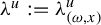 to be the inherited Riemannian volume measure on
$W^u(\omega ,x)$
 .
For
$l>1$
 , we define the (l-level) regular set

A point
$\omega \in \Omega $
 is called a generic point of
$\mathbb {P}$
 if
$({1}/{n})\sum _{i=0}^{n-1}\delta _{\theta ^i\omega }$
 converges to
$\mathbb {P}$
 in the weak
$^*$
 topology. We emphasize that, in the following theorem, the fiber manifold M may have arbitrary dimension with
$\dim M\geq 2$
 and the fiber maps are assumed only to be
$C^2$
 diffeomorphisms.
Theorem A. Assume that the skew-product transformation
$F : \Omega \, \times \, \mathcal {M} \to \Omega \, \times \, \mathcal {M}$
 is given as above. Let
$\mathbb {P}$
 be an ergodic
$\theta $
 -invariant measure on
$\Omega $
 . If there exists
$l>0$
 , a generic point of
$\mathbb {P}$
 , named
$\omega ^*$
 , and a Borel measurable set
$E_{\omega ^*}\subset W_{\mathrm {loc}}^u(\omega ^*,x_0)\cap \Lambda _l$
 with
$\lambda ^u_{(\omega ^*,x_0)}(E_{\omega ^*})>0$
 such that

then there exists a random SRB measure.
Remark 1.1. We refer to the conditions stated in Theorem A as the fiber leaf condition. Theorem A can be applied directly to the random perturbation of Axiom A basic sets, see [Reference Liu19]. When the external forcing of the skew product vanishes, our leaf condition coincides with that in [Reference Ben Ovadia4]. Consequently, we provide a new proof of the main results of [Reference Ben Ovadia4].
The key innovation of our approach is that, unlike previous constructions based on Young towers or any Markov structures, we rely purely on Burguet’s variational method adapted to the fiberwise recurrence context. The leaf condition guarantees that there exists an unstable leaf with a subset of positive leaf volume of hyperbolic points that are recurrent to a Pesin set with positive frequency. This subset gives the geometric set in Burguet’s paper. Using a Borel–Cantelli argument [Reference Burguet7, Lemma 2], we can construct a Følner sequence such that the geometric time is uniformly dense in this Følner sequence on a positive leaf volume subset. By averaging the leaf volume measure on the uniformity set along the Følner sequence, Burguet’s [Reference Burguet7, Lemma 4] can be applied to show that any limit measure has almost everywhere positive Lyapunov exponents. The crucial part is to show the Folner Gibbs property of the leaf volume measure, which guarantees the existence of SRB measure by [Reference Burguet7, Proposition 3].
Remark 1.2. Note that the leaf condition does not imply the continuity of the bundles
$E^u$
 and
$E^s$
 . Therefore, unlike in [Reference Burguet and Yang8], we must lift the measure to the Grassmannian bundle to estimate the metric entropy. To estimate the entropy of the random system, we establish a Gibbs–Følner property for random dynamical systems, see §2.4.
Our results also yield the existence of SRB measures for smooth skew-product systems (not random SRB measures). We assume further that
$\Omega $
 is a compact smooth manifold,
$\theta $
 is a
$C^{2}$
 diffeomorphism on
$\Omega $
 , and F is a
$C^{2}$
 diffeomorphism on
$\Omega \, \times \, \mathcal {M}$
 . Let
$\mathbb {P}$
 be a hyperbolic SRB measure of
$(\Omega ,\theta )$
 , and denote
$\lambda _{\theta ,\min }^+$
 and
$\lambda _{\theta ,\max }^-$
 to be the minimum of the positive Lyapunov exponents and the maximum of the negative Lyapunov exponents. The following theorem shows that, under the following spectral gap condition:

the random SRB measure lifts to an SRB measure for the entire skew product.
Theorem B. In the setting of Theorem A, assume further that
$\Omega $
 is a compact smooth manifold,
$\theta $
 is a
$C^{2}$
 diffeomorphism on
$\Omega $
 that admits an ergodic hyperbolic SRB measure
$\mathbb {P}$
 , and F is a
$C^{2}$
 diffeomorphism on
$\Omega \, \times \, \mathcal {M}$
 . If (1.4) holds, then there exists an SRB measure for the skew product F.
The rest of the paper is organized as follows. In §2, we collect the necessary preliminary lemmas. Section 3 contains the core of the paper: we adapt Burguet’s variational method to the random context. We construct an invariant random hyperbolic measure by averaging leaf-volume measures along suitably chosen Følner sequences and verify that it satisfies the fiber Følner Gibbs property. This property, combined with the subadditive ergodic arguments and the relative entropy estimates, yields the random SRB measure asserted in Theorem A. The proof of Theorem B is addressed in §4 and consists of two steps. In §4.1, we borrow ideas from [Reference Viana28, §4.2.5] to prove a dimension reduction lemma. In §4.2, we apply the dimension reduction lemma to prove that under the assumption (1.4), the positive Lyapunov exponents are exactly the positive Lyapunov exponents of
$(\Omega ,\theta ,\mathbb {P})$
 combining with the positive Lyapunov exponents generated by the RDS. Finally, we show that the entropy formula holds for a skew product system by using the Abramov–Rohlin formula and the random version of entropy formula.
2 Preliminary lemma
2.1 Invariant manifolds
The following lemma is a special version of [Reference Kifer and Liu15, Theorem 2.2.5] for random diffeomorphisms, see also [Reference Liu and Qian20, Theorem III.3.1].
Lemma 2.1. (Local stable and unstable manifolds)
For each
$n\in \mathbb {N}$
 and
$(\omega ,x)\in \Lambda _l$
 , there exists a continuous family of
$C^1$
 embedded k-dimensional discs
$W_{\mathrm {loc}}^s((\omega ,x),n)$
 and
$(\dim \mathcal {M}-k)$
 -dimensional discs
$W_{\mathrm {loc}}^u((\omega ,x),n)$
 in
$\mathcal {M}$
 , and there exist positive numbers
$\delta (l),\ L(l)\in (0,1)$
 and
$\zeta (l)$
 such that the following statements hold.
-
(a) There exists a $C^{1}$
map $$ \begin{align*} h_{(\omega,x),n}^s: O_n^s(\omega,x) \to & E^u(\theta^n\omega,f_\omega^n(x)),\\ h_{(\omega,x),n}^u:O_n^u(\omega,x) \to & E^s(\theta^n\omega,f_\omega^n(x)), \end{align*} $$where $O_n^\tau (\omega ,x)$
is an open subset of
$E^\tau (\theta ^n\omega ,f_\omega ^n(x))$
containing
$\{\xi \in E^\tau (\theta ^n\omega , f_\omega ^n (x)):\ |\xi |<\delta (l)e^{-\epsilon n}\}$
for
$\tau =s,u$
, such that:
-
(i) $ h_{(\omega ,x),n}^\tau (0)=0$
for
$\tau =s,u$
; -
(ii) $\mathrm {Lip}( h_{(\omega ,x),n}^\tau )\leq L(l)e^{\epsilon n}$
,
$\mathrm {Lip }(D_\cdot h_{(\omega ,x),n}^\tau )\leq L(l)e^{\epsilon n}$
for
$\tau =s,u$
; -
(iii) $W_{\mathrm {loc}}^\tau ((\omega ,x),n)=\exp _{f_\omega ^n(x)}\mathrm {Graph}(h_{(\omega ,x),n}^\tau )$
and tangent to
$E^\tau (\theta ^n\omega ,f_\omega ^n(x))$
at point
$f_\omega ^n(x)$
for
$\tau =s,u$
.
-
-
(b) We have $f_{\theta ^n\omega }W_{\mathrm {loc}}^s((\omega ,x),n)\subset W_{\mathrm {loc}}^s((\omega ,x),n+1)$
and
$(f_{\theta ^{n+1}\omega })^{-1}W_{\mathrm { loc}}^u((\omega ,x), n+1)\subset W_{\mathrm {loc}}^u((\omega ,x),n)$
. -
(c) We have $d^s(f_{\theta ^n\omega }^{t}(y),f_{\theta ^n\omega }^t(z))\leq \zeta (l)e^{\epsilon n}e^{(-\chi +\epsilon )t}d^s(y,z)$
for
$y,z\in W_{\mathrm { loc}}^s((\omega ,x),n)$
,
$t\in \mathbb {N}$
, where
$d^s$
denote the distance along
$W_m^s(\omega ,x)$
for
$m\in \mathbb {N}$
induced by the inherited Riemannian metric as submanifolds of
$\mathcal {M}$
. Here,
$d^u(f_{\theta ^n\omega }^{-t}(y),f_{\theta ^n\omega }^{-t}(z))\leq \zeta (l)e^{\epsilon n}e^{(-\chi +\epsilon )t}d^u(y,z)$
for
$y,z\in W_{\mathrm {loc}}^u((\omega ,x),n)$
,
$t\in \mathbb {N}$
, where
$d^u$
denotes the distance along
$W_m^u(\omega ,x)$
for
$m\in \mathbb {N}$
induced by the inherited Riemannian metric as submanifolds of
$\mathcal {M}$
.





From now on, we will use the following notation:
$ W_{\delta (l)}^\tau (\omega ,x):=W_{\mathrm {loc}}^\tau ((\omega ,x),0),$
 and
$h_{(\omega ,x)}^\tau :=h_{(\omega ,x),0}^\tau $
 for
$(\omega ,x)\in \Lambda _l$
 and
$\tau =s,u$
 . By statement (a) of Lemma 2.1, one has
$\delta (l)e^{-N\epsilon }\leq \delta (le^{N\epsilon })$
 for any
$N\in \mathbb {N}$
 . The following is a direct corollary of the local stable and unstable manifolds.
Corollary 2.1. For any given
$l>0$
 , there exists
$C(l)>0$
 such that for any
$8\delta <\delta (l)$
 , as in Lemma 2.1, and any
$(\omega ,x)\in \Lambda _l$
 , one has

2.2 Bounded distortion lemmas
For any
$(\omega ,x)\in \Lambda _l$
 , according to the definition of
$\Lambda _l$
 , we have that both
$(\theta \omega ,f_\omega (x))$
 and
$(\theta ^{-1}\omega ,f_\omega ^{-1}(x))$
 belong to
$\Lambda _{le^\epsilon }$
 . The idea of the following bounded distortion lemma comes from [Reference Lian, Liu and Lu18, Lemma 3.2].
Lemma 2.2. There exists positive numbers
$C_l$
 and
$\delta ^\prime (l)<\min \{\delta (le^\epsilon ),\delta (l)\}$
 such that for any
$(\theta \omega ,f_\omega (x))\in \Lambda _l$
 ,
$f_\omega (y)\in W_{\delta (l)}^u(\theta \omega ,f_\omega (x))$
 and
$y\in W^u_{\delta ^\prime (l)}(\omega ,x)$
 , one has

Proof of Lemma 2.2.
With the help of the normal coordinate chart, we deal with
$W_{\delta (le^\epsilon )}^{u}(\omega ,x)$
 and
$W^{u}_{\delta (l)}(\theta \omega ,f_\omega (x))$
 in Euclidean space. We let
$\delta ^\prime (l)<\delta (le^\epsilon )$
 be determined later. By Lemma 2.1, there exist
$ \xi _y\in E^{u}(\omega ,x)(\delta ^\prime (l)) $
 and
$ \xi _{f_\omega (y)}\in E^{u}(\theta \omega ,f_\omega (x))(\delta (l))$
 such that


and
$T_yW^u_{\delta (le^\epsilon )}(\omega ,x)=\mathrm {Graph}((Dh_{(x,\omega )}^{uu})_{\xi _y})$
 ,
$T_{f_\omega (y)}W^u_{\delta (l)}(\theta \omega ,f_\omega (x))= \mathrm {Graph} ((Dh^{uu}_{(f_\omega (x),\theta \omega )})_{\xi _{f_\omega (y)}})$
 . By (2.1) and (2.2), we have

and

so
$|\xi _{f_\omega (y)}|\leq R(({1+L(le^\epsilon )})/({1-L(l)}))|\xi _y|$
 , where
$R\geq 1$
 is a constant such that

Now, we define the following linear maps
$L_{(\omega ,x)}, \tilde {L}_{(\omega ,y)}:E^{u}(\omega ,x)\rightarrow E^{u}(\theta \omega ,f_\omega (x))$
 by

where
$\pi ^u_{(\theta \omega ,f_\omega (x))}$
 is the projection from
$T_{f_\omega (x)}\mathcal {M}$
 to
$E^u(\theta \omega ,f_\omega (x))$
 with respect to the splitting
$E^u(\theta \omega ,f_\omega (x))\oplus E^s(\theta \omega ,f_\omega (x))$
 . Note that
$(\theta \omega ,f_\omega (x))\in \Lambda _l$
 and
$\angle (E^u(\theta \omega ,f_\omega (x)),E^s(\theta \omega ,f_\omega (x)))\geq l^{-1}$
 , there exists
$\theta (l)>0$
 such that
$\|\pi ^u_{(\theta \omega ,f_\omega (x))}\|\leq \theta (l)$
 . Then,

Now, we have

Hence,
$\|L_{(\omega ,x)}-\tilde {L}_{(\omega ,y)}\|\leq C_0(R\theta (l)+R\theta (l)L(l))d^u(x,y)$
 , where
$C_0$
 only depends on the normal coordinate chart. Then, by the property of the determinant,

where
$C_1(l)$
 is a polynomial of
$R\theta (l)+R\theta (l)L(l)$
 and
$\dim E^{u}(\omega ,x)$
 .
Note that

Therefore,

where
$\delta ^\prime (l)$
 is chosen so that
$L(l)\cdot R(({1+L(le^\epsilon )})/({1-L(l)}))\delta ^\prime (l)<1/2.$
 So, we have

where
$C_2(l)$
 is a polynomial of
$L(l)\cdot R(({1+L(le^\epsilon )})/({1-L(l)}))$
 and
$\dim E^{u}(\omega ,x)$
 . In addition,

implies that there exists
$C_3(l)$
 such that

Combining (2.4), (2.5), and (2.6), we conclude that there exists
$C_4(l)>0$
 ,

Then, the proof of Lemma 2.2 is complete by letting
$C_l=C_4(l)/\sup _{(\omega ,x,E)}|\!\det D_xf_\omega |_{E}|$
 .
For any
$N\in \mathbb {N}$
 and
$\Delta \subset \Lambda _l(\omega )$
 , we say that an interval of integers
$[a,b]$
 is N-
$\{(\omega ,x):\ x\in \Delta \}$
 -admissible if for any
$x\in \Delta $
 , there exists a sequence of numbers
$a=a_0< a_1<\cdots <a_n=b$
 (depending on
$(\omega ,x)$
 ) such that
$(\theta ^{a_i}\omega ,f_\omega ^{a_i}(x))\in \Lambda _l$
 for
$i=0,\ldots ,n$
 and
$a_{i+1}-a_i\leq N$
 .
Lemma 2.3. For any
$N\in \mathbb {N}$
 ,
$\gamma>0$
 , there exists
$\delta _0(l,N,\gamma )>0$
 such that for any
$(\omega ,x)\in \Lambda _l$
 ,
$\delta <\delta _0(l,N,\gamma )$
 , for any
$n>0$
 with
$[0,n]$
 is N-
$\{(\omega ,x)\}$
 -admissible, one has:
-
(1) for any $0\leq i\leq n$
, the local unstable manifold
$W_{8\delta }^u(\theta ^i\omega ,f_\omega ^i(x))$
is well defined and $$ \begin{align*}f_\omega^i(W_{4\delta}^u(\omega,x)\cap B_n(\omega,x,\delta))\subset W_{4\delta}^u(\theta^i\omega,f_\omega^i(x));\end{align*} $$
-
(2) for any Borel measurable set $\Delta \subset W_{4\delta }^u(\omega ,x)\cap B_n(\omega ,x,\delta )$
, one has $$ \begin{align*} e^{-\gamma}\leq \frac{\lambda^u(\Delta)\det(D_xf_\omega^n|_{E^u(\omega,x)})}{\lambda^u(f_\omega^n(\Delta))}\leq e^{\gamma}. \end{align*} $$


Proof of Lemma 2.3.
For any
$(\omega ,x)\in \Lambda _l$
 and
$[0,n]$
 that is N-
$\{(\omega ,x)\}$
 -admissible, then by definition, there exists
$0=a_0<a_1<\cdots <a_k=n$
 with
$a_{i+1}-a_i\leq N$
 such that
$(\theta ^{a_i}\omega ,f_\omega ^{a_i}(x))\in \Lambda _l$
 for
$i=0,\ldots ,k$
 . Therefore, for any
$t\in [0,n]$
 , we have
$(\theta ^t\omega ,f_\omega ^t(x))\in \Lambda _{le^{N\epsilon }}$
 . As a consequence, for any

$W_{8\delta }^u(\theta ^t\omega ,f_\omega ^t(x))$
 is well defined, where
$\delta ^\prime (l)$
 is given in Lemma 2.2, and R is a constant as in (2.3).
For
$i\in [a_0,a_1]$
 , we have

As a consequence,
$f_\omega ^iW_{4\delta }^u(\omega ,x)$
 belongs to the local stable manifolds. Therefore, for
$i\in [a_0,a_1]$
 , we have

Inductively, one can prove statement (1) holds. Next, we prove statement (2).
For any Borel measurable set
$\Delta \subset W_{4\delta }^u(\omega ,x)\cap B_n(\omega ,x,\delta )$
 , by statement (1),
$f_\omega ^n(\Delta )\subset W_{4\delta }^u(\theta ^n\omega ,f_\omega ^n(x))$
 . Therefore,

By statement (1) and Lemma 2.2, we have estimate

where
$C_{le^{N\epsilon }}$
 is given in the statement of Lemma 2.2. This implies

The proof is complete by shrinking
$\delta $
 .
Lemma 2.4. For any
$N\in \mathbb {N}$
 and any
$\gamma>0$
 , there exists positive number
$\delta _1(l,N,\gamma )<\delta _0(l,N,\gamma )$
 such that for any
$\delta <\delta _1(l,N,\gamma )$
 ,
$(\omega ,x)\in \Lambda _l$
 , if
$y\in B_n(\omega ,x,\delta )$
 with
${}[\![ {} 0,n {}]\!] {}$
 being N-
$\{(\omega ,x),(\omega ,y)\}$
 -admissible, then we have

Proof of Lemma 2.4.
By the Hölder continuity of the fiber unstable subbundle (see e.g. [Reference Liu and Qian20, Ch. III, Theorem 4.1]), there exists a constant
$C(l)$
 such that for any
$(\omega ,z_1),(\omega ,z_2)\in \Lambda _{le^{N\epsilon }}$
 , one has

for some exponent
$\alpha \in (0,1)$
 . Note that
${}[\![ {} 0,n{}]\!] {}$
 is N-
$\{(\omega ,x),(\omega ,y)\}$
 -admissible, by the same argument in the proof of Lemma 2.3, for any
$i\in {}[\![ {} 0,n{}]\!] {}$
 ,
$(\theta ^i\omega ,f_\omega ^i(x))$
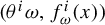 and
$(\theta ^i\omega ,f_\omega ^i(y))$
 belong to
$\Lambda _{le^{N\epsilon }}$
 . Then, the conclusion follows from the above inequality by letting

This completes the proof of this lemma.
2.3 Følner sequence
We introduce some notation of integers in this subsection and we use the same notation as in [Reference Burguet7]. We denote
$\mathcal {P}_{\mathbb {N}}$
 and
$\mathcal {P}_n$
 to be the power sets of
$\mathbb {N}$
 and
$\{0,1,2,\ldots ,n-1\}$
 ,
$n\in \mathbb {N}$
 . For
$a\leq b\in \mathbb {N}$
 , we write
${}[\![ {} a,b{}]\!] {}$
 (respectively
${}[\![ {} a,b{}[\ and
${}]\!] {} a,b{}]\!] {}$
 ) as the interval of integers k with
$a\leq k\leq b$
 (respectively
$a\leq k<b$
 and
$a<k\leq b$
 ). For any
$E\in \mathcal {P}_{\mathbb {N}}$
 , an interval of integers
${}[\![ {} a,b{}[\ is said to be E-irreducible if
$a,b\in E$
 and
${}[\![ {} a, b{}[\ . We denote
$E_M$
 to be the union of the intervals of integers
${}[\![ {} a,b{}[\ with
$a,b\in E$
 and
$0<b-a\leq M$
 . The boundary
$\partial E$
 of E is the symmetric difference of E and
$E+1$
 with
$E+1:=\{k+1,\ k\in E\}$
 . In particular,
$\partial {}[\![ {} a,b{}[\ . We denote
$\mathfrak {N}$
 to be the set of increasing sequences of natural integers. For
$\mathfrak {n}\in \mathfrak {N}$
 , the generalized power set of
$\mathfrak {n}$
 is defined by
$\mathcal {Q}_{\mathfrak {n}}:=\prod _{n\in \mathfrak {n}}\mathcal {P}_n$
 .
For
$n\in \mathbb {Z}^+$
 and
$E\in \mathcal {P}_{\mathbb {N}}$
 , we denote

The upper and lower asymptotic densities of
$E\in \mathcal {P}_{\mathbb {N}}$
 along a sequence
$\mathfrak {n}\in \mathfrak {N}$
 are defined by

We write
$d^{\mathfrak {n}}(E)$
 when
$\bar {d}^{\mathfrak {n}}(E)=\underline {d}^{\mathfrak {n}}(E)$
 . For
$\mathfrak {n}\in \mathfrak {N}$
 and
$\mathcal {F}=(F_n)_{n\in \mathfrak {n}}\in \mathcal {Q}_{\mathfrak {n}}$
 , we define

We write
$ d^{\mathfrak {n}}(\mathcal {F})$
 when
$ \bar {d}^{\mathfrak {n}}(\mathcal {F})= \underline {d}^{\mathfrak {n}}(\mathcal {F})$
 . The classical definition of Følner sequence only requires that
$\lim _{n\in \mathfrak {n}}(({\#\partial F_n})/{\# F_n})=0$
 . In this paper, we consider a stronger version of the Følner property.
Definition 2.1. For
$\mathfrak {n}\in \mathfrak {N}$
 and
$\mathcal {F}=(F_n)_{n\in \mathfrak {n}}\in \mathcal {Q}_{\mathfrak {n}}$
 , we let
$\partial \mathcal {F}:=(\partial F_n)_{n\in \mathfrak {n}}\in \mathcal {Q}_{\mathfrak {n}}$
 . We call
$\mathcal {F}$
 Følner if
$d^{\mathfrak {n}}(\partial \mathcal {F})=0$
 .
2.4 Relative entropy
We recall the definition of relative entropy in a general setting. In this section, we consider an RDS F over a metric dynamical system
$(\Omega ,\mathfrak {F},\mathbb {P},\theta )$
 on a compact metric space
$(X,\mathcal {B})$
 generated by
$g_\omega :X\to X$
 so that the map
$(\omega ,x)\mapsto g_\omega (x)$
 is measurable. We use the notation
$G(\omega ,x)=(\theta \omega ,g_\omega (x))$
 to denote the skew product transformation. For any Borel probability measure
$\mu $
 , on
$\Omega \, \times \, X$
 , a finite measurable partition
$\alpha ,\beta $
 of
$\Omega \, \times \, X$
 , and a
$\sigma $
 -sub-algebra
$\mathcal {B}_1$
 on
$\Omega \, \times \, X$
 , the conditional entropy function has the following property (see e.g. [Reference Liu and Qian20, Ch. 0]):
-
• $H_\mu (\alpha |\mathcal {B}_1)\leq \log \#\alpha $
,
$H_{\mu }(\alpha \vee \beta |\mathcal {B}_1)\leq H_{\mu }(\alpha |\mathcal {B}_1)+H_{\mu }( \beta |\mathcal {B}_1)$
; -
• $H_{\sum _{i}p_i\mu _i}(\alpha |\mathcal {B}_1)\geq \sum _{i}p_iH_{\mu _i}(\alpha |\mathcal {B}_1)$
for any probability measures
$\{\mu _i\}_{i=1}^n$
and probability vector
$\{p_i\}_{i=1}^n$
, see [Reference Kifer14]; -
• $H_{\mu }(G^{-1}\alpha |G^{-1}\mathcal {B}_1)=H_{G_*\mu }(\alpha |\mathcal {B}_1)$
. If
$\mathcal {B}_1$
is G-invariant, then
$H_{\mu }(G^{-1}\alpha |\mathcal {B}_1)=H_{G_*\mu }(\alpha |\mathcal {B}_1)$
.





For any G-invariant measure
$\mu $
 with marginal
$\mathbb {P}$
 on
$\Omega $
 , let
$\{\mu _\omega \}_{\omega \in \Omega }$
 be its disintegration. We recall that the relative entropy of G,
$h_\mu ^{(r)}(G)$
 , is defined by the following:

where the supremum is taken over all finite measurable partitions
$\mathcal {Q}$
 of
$\Omega \, \times \, X$
 in the form
$\mathcal {Q}=\{\Omega \, \times \, P_i\}$
 with a finite measurable partition
$\mathcal {P}=\{P_i\}$
 of X, and
$\mathfrak {F}_{\Omega \, \times \, X}$
 is the
$\sigma $
 -algebra formed by all sets
$A\, \times \, X$
 with
$A\in \mathfrak {F}$
 . Denote
$h_\mu (G)$
 to be the classical measure-theoretic entropy of skew product transformation G. There is the following Abramov–Rohlin formula [Reference Abramov and Rohlin1]:

Lemma 2.5. Let
$\mathcal {F}=(F_n)_{n\in \mathfrak {n}}$
 be a Følner sequence with
$\underline {d}^{\mathfrak {n}}(\mathcal {F})>0$
 . Then, for any finite measurable partition
$\mathcal {Q}$
 of
$\Omega \, \times \, X$
 and a fixed natural number q, there exists a sequence
$\epsilon _n=\epsilon _n(q,\#\mathcal {Q},\#F_n)\to 0$
 as
$n\in \mathfrak {n}\to \infty $
 such that for any
$n\in \mathfrak {n}$
 ,

where
$\{\mu _n\}_{n\in \mathfrak {n}}$
 is a sequence of Borel probability measures on
$\Omega \, \times \, X$
 .
Proof of Lemma 2.5.
We first consider the case where
$F_n={}[\![ {} n_0,n_1 {}]\!] {}$
 is an interval of integers. Fix a natural number
$q\in \mathbb {N}$
 . We consider the case where
$1<q\leq n_1-n_0$
 . For
$1\leq j\leq q-1$
 , we define
$a(j)=\lceil ({n_1-n_0-j}/{q})\rceil $
 . For any fixed
$j\in {}[\![ {} 0,q-1{}]\!] {}$
 , we have decomposition

where S has cardinality at most
$2q$
 . Therefore, we have

Summing the above over j from
$0$
 to
$q-1$
 and dividing it by
$ \#F_n$
 , we obtain

where the second inequality is due to the concavity of the conditional entropy. Then, dividing it by q, we obtain the desired inequality. Now, we consider the case where
$q> n_1-n_0$
 . By direct computation, we have

Now, we consider a general set
$F_n\in \mathcal {P}_n$
 , which can be decomposed into connected components
$F_n=\bigsqcup _{j\in J_n}F_n^j$
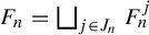 . Noticing that
$\#J_n\leq \#\partial F_n$
 , then we obtain

where the first inequality is due to the concavity of the conditional entropy function and the second inequality is due to the first case for intervals. Note that
$(F_n)_{n\in \mathfrak {n}}$
 is a Følner sequence with
$\underline {d}^{\mathfrak {n}}(\mathcal {F})>0$
 . Therefore, we have

2.5 Principle extension
For
$k\in \mathbb {N}$
 , we denote
$\mathcal {G}^k(T\mathcal {M}):=\bigsqcup _{x\in \mathcal {M}}\mathcal {G}^k(T_x\mathcal {M})$
 , where
$\mathcal {G}^k(T_x\mathcal {M})$
 is the Grassmannian that consists of all k-dim subspaces of
$T_x\mathcal {M}$
 . Let
$\mathcal {G}^k(T\Omega )$
 be denoted in the same way. Let

We denote

for any
$(x,E)\in \mathcal {G}^k(T\mathcal {M})$
 and let
$\mathbb {F}_\omega ^i$
 be generated as (1.1) by
$\mathbb {F}_\omega $
 . We note that
$\mathbb {F}$
 is isomorphic to the following map:

Both
$\tilde {F}$
 and
$\mathbb {F}$
 are extensions of F. Denote
$\pi :\Omega \, \times \, \mathcal {G}^k(T\mathcal {M}) \to \Omega \, \times \, \mathcal {M}$
 to be the natural projection. The following lemma says that both
$\tilde {F}$
 and
$\mathbb {F}$
 are principle extensions of F, whose proof basically follows the proof of [Reference Sun and Vargas27, Theorem 1.1].
Lemma 2.6. For any
$\mathbb {F}$
 -invariant Borel probability measure
$\mu $
 on
$\Omega \, \times \, \mathcal {G}^k(T\mathcal {M})$
 , one has
$h_{\mu }(\mathbb {F})=h_{\pi _*\mu }(F)$
 . As a consequence of the Abramov–Rohlin formula,

Proof of Lemma 2.6.
We denote
$E_k(x):=\Lambda ^k(T_x\mathcal {M})$
 and
$E_k=\bigsqcup _{x\in \mathcal {M}}E_k(x)$
 , where
$\Lambda ^k$
 is the kth exterior power. Let
$A_k:\mathcal {G}^0(T\Omega )\, \times \, E_k\to \mathcal {G}^0(T\Omega )\, \times \, E_k$
 be a vector bundle endomorphism over
$F:\Omega \, \times \, \mathcal {M}\to \Omega \, \times \, \mathcal {M}$
 and be defined by
$(A_k)_{(\omega ,x)}(0,e_1\wedge \cdots \wedge e_k)=(0,D_xf_\omega e_1\wedge \cdots \wedge D_xf_\omega e_k)$
 . Note that for any two bases
$\{e_1,\ldots ,e_k\}$
 and
$\{w_1,\ldots ,w_k\}$
 spanning the same k-dimensional subspaces of
$T_x\mathcal {M}$
 if and only if
$w_1\wedge \cdots \wedge w_k=ae_1\wedge \cdots \wedge e_k$
 for some
$a\in \mathbb {R}$
 , it gives an equivalence relation
$\sim $
 . Let
$D_k(x)=\{e_1\wedge \cdots \wedge e_k|\ e_1,\ldots ,e_k\text { be linearly independent in }T_x\mathcal {M}\}$
 and set
$G_k(x)=D_k(x)/\sim $
 ,
$G_k=\bigsqcup _{x\in \mathcal {M}}G_k(x)$
 . We note that

is a subbundle whose fiber over x is the projectivization of the set of decomposable k-vectors in
$E_k(x)$
 . We note that
$\mathcal {G}^k(T_x\mathcal {M})$
 is isomorphic to
$G_k(x)$
 by

Moreover, this isomorphism conjugates
$\tilde {F}$
 to
$P(A_k):P(\mathcal {G}^0(T\Omega ))\, \times \, G_k\subset P(\mathcal {G}^0(T\Omega )\, \times \, E_k)\to P(\mathcal {G}^0(T\Omega ))\, \times \, G_k$
 over F, which is defined by
$P(A_k)_{(\omega ,x)}([0]\, \times \, [e_1\wedge \cdots \wedge e_k])=[0]\, \times \, [D_xf_\omega e_1\wedge \cdots \wedge D_xf_\omega e_k]$
 . Now, for any
$\mathbb {F}$
 -invariant Borel probability measure
$\mu $
 on
$\Omega \, \times \, \mathcal {G}^k(T\mathcal {M})$
 , let
$\hat {\mu }$
 be the corresponding
$\tilde {F}$
 -invariant Borel probability measure on
$\mathcal {G}^0(T\Omega )\, \times \,\mathcal {G}^k(T\mathcal {M})$
 , and
$\hat {\mu }^*$
 be the
$P(A_k)$
 -invariant Borel probability measure on
$P(\mathcal {G}^0(T\Omega ))\, \times \, G_k$
 by conjugation. Then, the projection of
$\hat {\mu }^*$
 on
$\Omega \, \times \, \mathcal {M}$
 is
$\pi _*\mu $
 . By [Reference Sun and Vargas27, Theorem 3.7], we have
$ h_{\mu }(\mathbb {F})=h_{\hat {\mu }^*}(P(A_k))=h_{\pi _*\mu }(F).$

3 The existence of the random SRB measures
3.1 Construction of the invariant measure
By assumption (1.3), we can assume that
$E_{\omega ^*}\subset W_{\mathrm {loc}}^u(\omega ^*,x_0)$
 with
$\lambda ^u(E_{\omega ^*})>0$
 and there exists
$\beta _0>0$
 such that

Let
$T\in \mathbb {N}$
 to be determined later. Furthermore, we can assume that
$E_{\omega ^*}\subset W_{\mathrm {loc}}^u(\omega ^*,x_0)$
 with
$\lambda ^u(E_{\omega ^*})>0$
 , and there exist
$\beta :=\beta _{0}/T>0$
 and
$t\in \{0,\ldots ,T-1\}$
 such that

Denote
$I(\omega ^*,x):=I_{T}(\omega ^*,x)=\{j\in \{t+T\mathbb {N}\}: (\theta ^j\omega ^*,f_{\omega ^*}^j(x))\in \Lambda _l\}$
 for any
$x{\kern-1pt}\in{\kern-1pt} E_{\omega ^*}$
 . The following lemma is a direct corollary of [Reference Burguet7, Lemma 2].
Lemma 3.1. There exists
$\mathfrak {n}\in \mathfrak {N}$
 , Borel measurable subsets
$(A_n^{\omega ^*})_{n\in \mathfrak {n}}$
 of
$E_{\omega ^*}$
 and
$\mathcal {F}=\{F_n\}_{n\in \mathfrak {n}}\in \mathfrak {Q}_{\mathfrak {n}}$
 with
$\partial F_n\subset I(x)$
 for all
$x\in A_n^{\omega ^*}$
 ,
$n\in \mathfrak {n}$
 such that:
-
• $\lambda ^u(A_n^{\omega ^*})\geq {e^{-n\delta _n}}/{n^2}$
for all
$n\in \mathfrak {n}$
with
$\delta _n\to 0$
as
$n\in \mathfrak {n}\to \infty $
; -
• $\mathcal {F}$
is a Følner sequence; -
• I is dense in $\mathcal {F}$
uniformly on
$A_n^{\omega ^*}$
, that is, $$ \begin{align*} \limsup_{n\in\mathfrak{n}}\sup_{x\in A_n^{\omega^*}}d_n(F_n\backslash I_M(\omega^*,x))\to 0\quad\text{as }M\to\infty, \end{align*} $$where $I_M(\omega ^*,x)$
is the union of the interval of integers
${}[\![ {} a,b{}[\


The following is the main result in this section, which basically follows the idea of [Reference Burguet7, Lemma 4].
Proposition 3.1. Let
$\mu _n=\lambda ^u|_{A_n^{\omega ^*}}/\lambda ^u(A_n^{\omega ^*})$
 . There exists a limit measure of
$\{({1}/{\# F_n})\sum _{k\in F_n}F_*^k(\delta _{\omega ^*}\, \times \, \mu _n)\}_{n\in \mathfrak {n}}$
 , named
$\mu $
 , which is F-invariant with marginal
$\mathbb {P}$
 on
$\Omega $
 . Moreover, for
$\mu $
 -a.e.
$(\omega ,x)\in \Omega \, \times \, \mathcal {M}$
 , there are k positive Lyapunov exponents greater than
$\chi /2$
 , and
$\dim \mathcal {M}-k$
 negative Lyapunov exponents less than
$-\chi /2$
 .
Proof of Proposition 3.1.
Denote
$\mathbb {A}_n^{\omega ^*}=\{(\omega ^*,x,E^u(\omega ^*,x)):\ x\in A_n^{\omega ^*}\}$
 ,
$\mathbb {E}_{\omega ^*}=\{(\omega ^*,x,E^u(\omega ^*,x)):\ x\in E_{\omega ^*}\}$
 , and let
$\hat {\mu }_n$
 be the measure on
$\mathbb {A}_n^{\omega ^*}$
 corresponding to
$\mu _n$
 on
$A_n^{\omega ^*}$
 .
Let
$\mathfrak {n}^\prime $
 be a subsequence of
$\mathfrak {n}$
 such that
$\{\hat {\mu }_n^{F_n}:=({1}/{\# F_n})\sum _{k\in F_n}\mathbb {F}_*^k\hat {\mu }_n\}_{n\in \mathfrak {n}^\prime }$
 is converging to
$\hat {\mu }$
 under the weak
$^*$
 topology. By the property of the Følner sequence and a standard argument, one can see that
$\hat {\mu }$
 is
$\mathbb {F}$
 -invariant. Since
$F:\Omega \, \times \, \mathcal {M}\to \Omega \, \times \, \mathcal {M}$
 is a factor system of
$\mathbb {F}$
 , the projection of
$\hat {\mu }$
 is F-invariant. The projection of
$\hat {\mu }$
 has marginal
$\mathbb {P}$
 on
$\Omega $
 since
$\omega ^*$
 is a generic point of
$\mathbb {P}$
 .
For
$(\omega ,x,E)\in \mathcal {G}^0(T\Omega )\, \times \, \mathcal {G}^k(T\mathcal {M})$
 , we define
$\phi _n(\omega ,x,E)=\log m(D_xf_\omega ^n|_E)$
 for any
$n\in \mathbb {N}$
 , where m denotes the conorm. Then,
$\phi _n$
 is a continuous function on
$\mathcal {G}^0(T\Omega )\, \times \, \mathcal {G}^k(T\mathcal {M})$
 . Moreover, one has

Recall the definition of
$I(\omega ^*,x):=I_{T}(\omega ^*,x)$
 . We can pick T sufficiently large such that for any
$q>p\in I(\omega ^*,x)$
 and
$(\omega ^*,x,E^u(\omega ^*,x))\in \mathbb {E}_{\omega ^*}$
 ,

In fact, for any
$q>p\in I(\omega ^*,x)$
 , then
$q-p\geq T$
 and
$F^p(\omega ^*,x)\in \Lambda _l$
 ; therefore, we have

by picking T sufficiently large.
For convenience, define
$\phi _n^\prime (\omega ^*,x,E)=\phi _n(\omega ^*,x,E)-n\cdot ({\chi }/{2})$
 for
$n\in \mathbb {N}$
 . For a finite subset of integers J, we denote
$\phi _J(\omega ^*,x,E)$
 (respectively
$\phi _J^\prime (\omega ^*,x,E)$
 ) to be the sum of
$\phi _{q-p}(\mathbb {F}^p(\omega ^*,x,E))$
 (respectively
$\phi _{q-p}^\prime (\mathbb {F}^p(\omega ^*,x,E))$
 ), where
${}[\![ {} p,q{}[\ runs over all maximal intervals of integers contained in J. Finally, define
$\| \phi ^\prime _1\|_{\sup }:=\sup _{(\omega ,x,E)\in \mathcal {G}^0(T\Omega )\, \times \, \mathcal {G}^k(T\mathcal {M})}|\phi ^\prime _1(\omega ,x,E)|$
 .
Fix
$\alpha <0$
 ,
$M<N\in \mathbb {N}$
 . For
$x\in A_n^{\omega ^*}$
 ,
$n\in \mathfrak {n}^\prime $
 , we define

For
$l\in \mathbb {N}$
 and
$k\in \{0,\ldots ,N-1\}$
 with
$k+lN\in F_n$
 , define
$J_{k,l}= [k+lN,k+(l+1)N)\cap \mathbb {N}$
 . The interval of integers
$J_{k,l}$
 can be written as
$J_{k,l}=I_{k,l}^1(x)\sqcup I_{k,l}^2(x)\sqcup I_{k,l}^3(x)\sqcup I_{k,l}^4(x)$
 , where we have the following:
-
• $I_{k,l}^1(x)$
is the union of disjoint
$I(\omega ^*,x)$
irreducible interval of length less than M contained in
$J_{k,l}$
; by (3.1), we have
$\phi _{I_{k,l}^1}^\prime (\omega ^*,x,E^u(\omega ^*,x))\geq 0$
; -
• $I_{k,l}^2(x)$
consists of subintervals of an
$I(\omega ^*,x)$
irreducible interval of length less than M, which does not lie in
$J_{k,l}$
, but may contain the right extreme of
$J_{k,l}$
; in particular,
$\#I_{k,l}^2\leq 2M$
and, therefore,
$\phi _{I_{k,l}^2}^\prime (\omega ^*,x,E^u(\omega ^*,x))\geq -2M\| \phi ^\prime _1\|_{\sup }$
; -
• $I_{k,l}^3(x)\subset F_n\backslash I_M(\omega ^*,x)$
; -
• $I_{k,l}^4(x)\subset \mathbb {N}\backslash F_n$
.


Fix
$0\leq k<N$
 . Since
$k+lN\in F_n$
 , if
$I_{k,l}^4(x)\not =\emptyset $
 , then
$J_{k,l}$
 must contain a point of
$\partial F_n$
 . By the intervals
$\{J_{k,l}\}_l$
 are pairwise disjoint, we have
$\#(\bigcup _{l:~I_{k,l}^4(x)\not =\emptyset }J_{k,l})\leq N\cdot \#\partial F_n$
 . Therefore, by the superadditivity of
$\phi ^\prime $
 , for the fixed k, we obtain

If
$I_{k,l}^4(x)=\emptyset $
 , by the superadditivity of
$\phi ^\prime $
 , we obtain

As
$F_n\subset \{0,\ldots ,n-1\}$
 , the cardinality of
$\{l:\ k+lN\in F_n\}$
 is less than or equal to
$\lceil {n}/{N}\rceil $
 . Also by
$\{J_{k,l}\}_l$
 are pairwise disjoint,
$\sum _{\ell }\# I_{k,l}^3\leq \#(F_n\backslash I_M(\omega ^*,x))$
 . Therefore, we have

Combining these two cases, for each fixed
$0\leq k<N$
 , we have

For each
$(\omega ^*,x,E^u(\omega ^*,x))\in \mathbb {A}_n^{\omega ^*}$
 , define
$\delta _{(\omega ^*,x,E^u(\omega ^*,x))}^{F_n}=({1}/{\#F_n})\sum _{j\in F_n}\mathbb {F}_*^k \delta _{(\omega ^*,x,E^u(\omega ^*,x))}$
 . Note that (recall that
$\phi ^{\prime }_{J_{k,l}}=\phi ^{\prime }_N$
 )

By (3.2), after summing over
$k\in \{0,\ldots ,N-1\}$
 ,

Hence, dividing by
$N\cdot \#F_n$
 , we have

Recall that
$\hat {\mu }_n$
 is supported on
$\mathbb {A}_n^{\omega ^*}$
 . We integrate with
$\hat {\mu }_n^{F_N}$
 , then

Note that
$\{{\phi _N^\prime }/{N}\leq \alpha \}$
 is closed, so by weak
$^*$
 convergence, we have

Note that
$\alpha <0$
 ; therefore, we get for all M:

By taking M to infinity, we arrive at
$\lim _{N\to \infty }\hat {\mu }\{{\phi _N^\prime }/{N}\leq \alpha \}=0$
 by Lemma 3.1. Therefore,
$\lim _{N\to \infty }({\phi _N^\prime }/{N})=\lim _{N\to \infty }({\phi _N}/{N})-{\chi }/{2}\geq \alpha $
 for
$\hat {\mu }$
 -a.e
$(\omega ,x,E)\in \mathcal {G}^0(T\Omega )\, \times \, \mathcal {G}^k(T\mathcal {M})$
 , where the limit exists due to the Kingman’s subadditive ergodic theorem. Since
$\alpha <0$
 is arbitrary, we conclude that

For
$(\omega ,x,E)\in \mathcal {G}^0(T\Omega )\, \times \, \mathcal {G}^{(\dim \mathcal {M}-k)}(T\mathcal {M})$
 , we define
$\psi _n(\omega ,x,E)= \log \|D_x f_\omega ^n|_E\|^{-1}$
 . Then,
$\psi _n$
 is a continuous function on
$\mathcal {G}^0(T\Omega )\, \times \, \mathcal {G}^{(\dim \mathcal {M}-k)}(T\mathcal {M})$
 . It is clear that
$ \psi _{n+m}(\omega ,x,E)\geq \psi _n(\omega ,x,E)+\psi _m(\mathbb {F}^n(\omega ,x,E)).$
 Denote
$\bar {E}_{\omega ^*}=\{(\omega ^*,x,E^s (\omega ^*,x)):\ x\in E_{\omega ^*}\}$
 and
$\bar {A}_n^{\omega ^*}=\{(\omega ^*,x,E^s(\omega ^*,x)):\ x\in A_n^{\omega ^*}\}$
 . We let
$\bar {\mu }_n$
 be the measure on
$\bar {A}_n^{\omega ^*}$
 corresponding to
$\mu _n$
 on
$A_n^{\omega ^*}$
 . Note that for any
$q>p\in I(\omega ^*,x)$
 , then
$q-p\geq T$
 and
$F^p(\omega ^*,x)\in \Lambda _l$
 ; therefore, we have

By the same proof as (3.3), for any
$\mathfrak {n}^{\prime \prime }$
 being a subsequence of
$\mathfrak {n}^{\prime }$
 such that
$\{({1}/{\# F_n})\sum _{k\in F_n}\mathbb {F}_*^k\bar {\mu }_n\}_{n\in \mathfrak {n}^{\prime \prime }}$
 converges to
$\bar {\mu }$
 , one has

By the construction, we have

We name
$Pro\hspace {-1pt}j_{\Omega \, \times \, \mathcal {M}}(\hat {\mu })$
 by
$\mu $
 , and this measure has marginal
$\mathbb {P}$
 on
$\Omega $
 since
$\omega ^*$
 is a generic point of
$\mathbb {P}$
 . We conclude from (3.3) and (3.4) that for
$\mu $
 -a.e.
$(\omega ,x)\in \Omega \, \times \, \mathcal {M}$
 , there are k positive Lyapunov exponents greater than
$\chi /2$
 and
$\dim \mathcal {M}-k$
 negative Lyapunov exponents less than
$-\chi /2$
 . The proof of Proposition 3.1 is complete.
3.2 Fiber Følner Gibbs property
In this subsection, we prove the fiber Følner Gibbs property. Recall that
$\{A_n^{\omega ^*}\}_{n\in \mathfrak {n}}$
 and
$\mathcal {F}=\{F_n\}_{n\in \mathfrak {n}}$
 are given in Lemma 3.1. We first denote

Fix
$\gamma>0$
 . For each
$M>0$
 , let
$\delta _1=\delta _1(l,M,\gamma )$
 be defined as in Lemma 2.4 and let
$C(l)$
 be given in Corollary 2.1. We denote

By direct computation, one can see that for fixed l and
$\gamma $
 ,

Then, we have

Proposition 3.2. For any
$n\gg M$
 , any finite measurable partition
$\mathcal {P}$
 of M with

and any
$x\in A_n^{\omega ^*}$
 , one has

where
$\mathcal {P}_{\omega ^*}^{F_n}=\bigvee _{i\in F_n}(f_{\omega ^*}^i)^{-1}\mathcal {P}$
 and
$J^u(f_{\omega ^*}^i(x)):=\log |\!\det (D_{f_{\omega ^*}^i(x)}f_{\theta ^i(\omega ^*)}|_{E^u(\theta ^i\omega ^*,f_{\omega ^*}^i(x))}) |$
 for
$i\in F_n$
 .
Proof of Proposition 3.2.
For any
$x\in E_{\omega ^*}$
 ,
$M>0$
 , and any
$n\gg M$
 , let
$L_n(\omega ^*,x)\subset I(\omega ^*,x)\cap {}[\![ {}0,n{}[\ be the disjoint union of
$\{a,b\}$
 satisfying

Denote
$n_{(\omega ^*,x)}$
 to be the number of pairs in
$L_n(\omega ^*,x)$
 . By (3.8), we have
$n_{(\omega ^*,x)}\leq \lceil {n}/{M}\rceil $
 and, therefore,

We consider
$S_n=\{\bigsqcup _{i=1}^k\{a_i,b_i\}|\ b_i-a_i>M,\ k\leq \lceil {n}/{m}\rceil \}$
 , that is, all the possibilities of
$L_n(\omega ^*,x)$
 . When n is sufficiently large, one has

For any
$s\in S_n$
 , we denote
$A_{n,s}^{\omega ^*}=\{z\in A_n^{\omega ^*}|\ L_n(x)=s\in S_n\}$
 . Then, for any
$x\in A_{n}^{\omega ^*}$
 ,

Next, we are going to estimate the right side of the above inequality for fixed
$x\in A_{n}^{\omega ^*}$
 .
Recall that
$I_M(\omega ^*,x)$
 is the union of the intervals
${}[\![ {} c,d{}[\ with
$c,d\in I(\omega ^*,x)$
 and
$0<d-c\leq M$
 . Fix
$s=\bigsqcup _{i=1}^k\{a_i,b_i\}$
 and for any
$x\in A_{n,s}^{\omega ^*}$
 , we let
$I_M(s)=I_M(\omega ^*,x)\cap {}[\![ {} 0,n{}[\ . By the definition of
$A_{n,s}^{\omega ^*}$
 , we have

We decompose
$F_n$
 into the following two parts:
-
• $F_{n,s}^2:=F_n\backslash I_M(s)$
; -
• $F_{n,s}^1:= F_n\backslash F_{n,s}^1=\bigcup _{i=0}^{m_s-1}{}[\![ {} c_i,d_i{}]\!] {}$
.


Without loss of generality, we can assume
$0\in F_n$
 for all
$n\in \mathfrak {n}$
 and, therefore,
$C_0=0$
 . Note that
$F_{n,s}^1=F_n\cap I_M(s)$
 ; therefore, for any
$0\leq i\leq m_s-1$
 ,
${}[\![ {} c_i,d_i{}]\!] {}$
 is M-
$\{(\omega ^*,x):\ x\in A_{n,s}^{\omega ^*}\}$
 -admissible and

Claim 3.1. There exists a constant
$\tilde {C}>0$
 such that for any
$x_s\in A_{n,s}^{\omega ^*}\cap P_{\omega ^*}^{F_n}(x)$
 , one has

where
$\mathcal {P}_{\omega ^*}^{F_{n,s}^1}=\bigvee _{i\in F_{n,s}^1}(f_{\omega ^*}^i)^{-1}\mathcal {P}$
 .
Proof of Claim 3.1.
The first inequality is clear; therefore, we only need to prove the second inequality. For
$k\in {}[\![ {} 0,m_s-1{}]\!] {}$
 , we denote
$F_{n,s}^1(k):=\bigcup _{i=0}^k{}[\![ {} c_i,d_i{}]\!] {}$
 .
Step 1. When
$k=0$
 , we are going to estimate
$\lambda ^u(A_{n,s}^{\omega ^*}\cap P_{\omega ^*}^{F_{n,s}^1(0)}(x))$
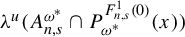 . Note that
${}[\![ {} c_0,d_0{}]\!] {}={}[\![ {} 0, d_0{}]\!] {}$
 is M-
$\{(\omega ^*,x):\ x\in A_{n,s}^{\omega ^*}\}$
 -admissible. Denote
$\Delta _0=A_{n,s}^{\omega ^*}\cap \mathcal {P}_{\omega ^*}^{F_{n,s}^1(0)}(x)$
 . By Lemma 2.3 and diam
$(\mathcal {P})<\delta $
 , and note that
$x_s\in A_{n,s}^{\omega ^*}\cap P_{\omega ^*}^{F_n}(x)$
 , we have

Then, we have

Step 2. We consider the case of
$k=1$
 . Denote
$\Delta _1=A_{n,s}^{\omega ^*}\cap \mathcal {P}_{\omega ^*}^{F_{n,s}^1(1)}(x)$
 , then

In addition, note that
${}[\![ {} c_1,d_1{}]\!] {}$
 is M-
$\{(\omega ^*,x):\ x\in A_{n,s}^{\omega ^*}\}$
 -admissible; therefore, we have

Then, there exists finite points
$\{y_i^1\}_{i\in I_1}\subset f_{\omega ^*}^{d_0}(\Delta _1)$
 such that:
-
(1) $W_{4\delta }^u(\theta ^{c_1}\omega ^* ,f_{\theta ^{d_0}\omega ^*}^{c_1-d_0}y_i^1)$
are mutually disjoint; and -
(2) $f_{\omega ^*}^{d_0}(\Delta _1)\subset \bigcup _{i\in I_1}f_{\theta ^{c_1}\omega ^*}^{-(c_1-d_0)}(W_{4\delta }^u(\theta ^{c_1}\omega ^*,f_{\theta ^{d_0}\omega ^*}^{c_1-d_0}(y_i^1))\cap B(f_{\omega ^*}^{c_1}x_s,\delta ))\subset W_{8\delta }^u(\theta ^{d_0}\omega ^*, f_{\omega ^*}^{d_0}(x_s))$
.


We denote
$\Delta _1^i(\theta ^{c_1}\omega ^*){\kern-1pt}={\kern-1pt}f_{\omega ^*}^{c_1}(\Delta _1){\kern-1pt}\cap{\kern-1pt} W_{4\delta }^u(\theta ^{c_1}\omega ^* ,f_{\theta ^{d_0}\omega ^*}^{c_1-d_0}(y_i^1)){\kern-1pt}\cap{\kern-1pt} B(f_{\omega ^*}^{c_1}(x_s),\delta )$
 for
${i{\kern-1.2pt}={\kern-1.2pt}1{\kern-1.2pt}\in{\kern-1.2pt} I_1}$
 , and by the choice of
$\{y_i^1\}_{i\in I_1}$
 ,

We note that
${}[\![ {} 0,d_1-c_1{}]\!] {}$
 is M-
$\{(\theta ^{c_1}\omega ^*,x):\ x\in \Delta _1^i(\theta ^{c_1}\omega ^*)\}$
 -admissible. Applying Lemma 2.3 on
$\Delta _1^i(\theta ^{c_1}\omega ^*)$
 , we have

and

where the second inequality is due to Corollary 2.1 and the third inequality is due to Lemma 2.4. Note that
$\sum _i\lambda ^u(f_{\theta ^{c_1}\omega ^*}^{-(c_1-d_0)}W_{4\delta _1}^u(\theta ^{c_1}\omega ^*,f_{\theta ^{d_0}\omega ^*}^{c_1-d_0}(y_i^1)))\leq \lambda ^u(W_{8\delta _1}^u(\theta ^{d_0}\omega ^*, f_{\omega ^*}^{d_0}(x_s))) \leq ~1$
 and

where the first inequality is due to Lemma 2.4 and the second inequality is due to (3.7). The inequality (3.14) enables us to estimate the sum of determinants in the gaps of
$F_{n,s}^1(1)$
 , that is,

Then, we have estimates

Then, finally, we have

Step 3. We consider the case
$k=2$
 . Denote
$\Delta _2=A_{n,s}^{\omega ^*}\cap \mathcal {P}_{\omega ^*}^{F_{n,s}^1(2)}(x)=\Delta _1\cap \mathcal {P}_{\omega ^*}^{{}[\![ {} c_2,d_2{}]\!] {}}(x)$
 . Notice that
${}[\![ {} c_2,d_2{}]\!] {}$
 is M-
$\{(\omega ^*,x):\ x\in A_{n,s}^{\omega ^*}\}$
 -admissible, and

then
$\text {for all } j\in I_1$
 , there exist finite points
$\{z_i^{j,2}\}_{i\in I_{j,2}}\subset f_{\omega ^*}^{d_0}\Delta _2$
 such that
$\{W_{4\delta }^u(\theta ^{c_2}\omega ^*, f_{\theta ^{d_0}\omega ^*}^{c_2-d_0}(z_i^{j,2}))\}_{i\in I_{j,2}}$
 are mutually disjoint, and

For
$j\in I_1$
 and
$i\in I_{j,2}$
 , we denote

Now,
$\bigcup _{i\in I_{j,2}}\Delta _1^{j,i}(\theta ^{c_1}\omega ^*)$
 is in the position of
$\Delta _1$
 in Step 2. By the similar estimates, we obtain

Then,

Similar as (3.16), we obtain

Repeating the above procedure, we can obtain

The proof of Claim 3.1 is complete.
Note that for
$x\in A_n^{\omega ^*}$
 ,
$I_M(\omega ^*,x)$
 may not coincide with
$I_M(s)$
 . For the
$x_s$
 in the statement of Claim 3.1 and note that
$x_s\in A_{n,s}^{\omega ^*}\cap P_{\omega ^*}^{F_n}(x)$
 , moreover for those
$i\in I_M(\omega ^*,x)\cap I_M(\omega ^*,x_s)$
 , one has
$(\theta ^i\omega ^*,f_{\omega ^*}^i(x))$
 and
$(\theta ^i\omega ^*,f_{\omega ^*}^i(x_s))$
 both belong to
$\Lambda _{le^{M\epsilon }}$
 . Then, by Lemma 2.4, for those
$i\in I_M(\omega ^*,x)\cap I_M(\omega ^*,x_s)$
 , one has

For those i such that it may not satisfy the above estimate, we also have estimates

Combining the above two cases, we obtain

Therefore, for
$x\in A_{n}^{\omega ^*}$
 and
$x_s\in A_{n,s}^{\omega ^*}\cap P_{\omega ^*}^{F_n}(x)$
 , we have

By (3.10) and (3.9), when
$n\gg M$
 , we have

The proof of Proposition 3.2 is complete.
3.3 Entropy formula
In this subsection, we estimate the relative entropy of
$\mu $
 constructed in Proposition 3.1. Let us first recall some notation from Proposition 3.1. We recall that
$\mathbb {A}_n^{\omega ^*}=\{(\omega ^*,x,E^u(\omega ^*,x)):\ x\in A_n^{\omega ^*}\}$
 and let
$\hat {\lambda }^u$
 be the measure concentrated on
$\mathbb {A}_n^{\omega ^*}$
 corresponding to
$\lambda ^u$
 on
$A_{n}^{\omega ^*}$
 , that is,

We recall that
$\mu _n=\lambda ^u|_{A_n^{\omega ^*}}/\lambda ^u(A_n^{\omega ^*})$
 and
$\hat {\mu }_n=\hat {\lambda }^u/\hat {\lambda }^u(\mathbb {A}_n^{\omega ^*}).$
 Note that
$\hat {\mu }_n$
 is concentrated on the fiber
$\{\omega ^*\}$
 and then
$\hat {\mu }_n$
 has disintegration

We recall that in the proof of Proposition 3.1,
$\hat {\mu }$
 is the weak
$^*$
 limit of
$\{({1}/{\# F_n})\sum _{k\in F_n}\mathbb {F}_*^k \hat {\mu }_n\}_{n\in \mathfrak {n}^{\prime \prime }}$
 ,
$\mu =Pro\hspace {-1pt}j_{\Omega \, \times \, \mathcal {M}}(\hat {\mu })$
 and here,
$\mathfrak {n}^{\prime \prime }$
 is a subsequence of
$\mathfrak {n}$
 .
For any
$\gamma>0$
 , by (3.6) and the third item of Lemma 3.1, we can pick M sufficiently large such that

and

Pick any finite measurable partition
$\mathcal {P}=\{P_i\}$
 of
$\mathcal {M}$
 with

as in Proposition 3.2. Denote
$\hat {\mathcal {P}}=\{\pi ^{-1}(\Omega \, \times \, P_i)\}$
 to be a corresponding measurable partition of
$\Omega \, \times \, \mathcal {G}^k(T\mathcal {M})$
 , where
$\pi :\Omega \, \times \, \mathcal {G}^k(T\mathcal {M})\to \Omega \, \times \, \mathcal {M}$
 is the natural projection. We can pick
$\mathcal {P}$
 such that

By Proposition 3.2, for any
$x\in A_n^{\omega ^*}$
 and
$E\in \mathcal {G}^k(T_x\mathcal {M})$
 , one has

Let
$n\gg M\gg m$
 . By [Reference Ledrappier and Walters16, Lemma 3.2 (ii)], we have

To apply [Reference Ledrappier and Walters16, Lemma 3.2 (ii)], we use the fact that in (3.21),
$\Omega $
 is a compact metric space and
$\mathcal {F}_{\Omega \, \times \, \mathcal {G}^k(T\mathcal {M})}$
 is the
$\sigma $
 -algebra formed by all sets
$A\, \times \, \mathcal {G}^k(T\mathcal {M})$
 with
$A\in \mathcal {B}(\Omega )$
 . Using Lemma 2.5, we obtain

Note that
$\hat {\mu }_n$
 has disintegration by (3.20), so by the definition of conditional entropy,

where we recall
$\mathbb {F}_\omega ^i$
 is generated by (2.9), and here, partition
$\hat {\mathcal {P}}(\theta ^i\omega ^*)$
 equal to the projection of
$\hat {\mathcal {P}}$
 on
$\mathcal {G}^k(T\mathcal {M})$
 for all
$i\in \mathbb {Z}$
 . Then, by the definition of entropy, we have

By the first item of Lemma 3.1 and the fourth item
$\underline {d}^{\mathfrak {n}}(\mathcal {F})\geq \beta>0$
 , we have

By (3.22), the third item of Lemma 3.1, and direct computation, one can deduce that

where in the last inequality, we use the continuity of
$\log |\!\det (D_xf_\omega |_{E})| $
 on
$\Omega \, \times \, \mathcal {G}^k(T\mathcal {M})$
 , and in the last equality, we use (3.3). Since
$\gamma $
 is arbitrary, we have

Letting
$m\to \infty $
 , we obtain

By Ruelle’s inequality for RDS (see [Reference Kifer and Liu15, Theorem 3.1.1]), we obtain

that is,
$\mu $
 is a random SRB measure.
4 The existence of SRB measure
In this section, we assume that
$\Omega $
 is a closed smooth manifold and
$\theta $
 is a
$C^{2}$
 diffeomorphism on
$\Omega $
 that admits an ergodic hyperbolic SRB measure
$\mathbb {P}$
 , and F is a
$C^{2}$
 diffeomorphism on
$\Omega \, \times \, \mathcal {M}$
 . We assume (1.4) holds, that is,

Let
$\mu $
 be any random SRB measure with marginal
$\mathbb {P}$
 on
$\Omega $
 obtained in Theorem A. We are going to show that
$\mu $
 is an SRB measure for F. Since
$\mathbb {P}$
 is an SRB measure, we denote
$T_\omega \Omega =H^u(\omega )\oplus H^s(\omega )$
 to be the Oseledets splitting corresponding to positive and negative Lyapunov exponents, and we denote
$P(H^u(\omega ))$
 and
$P(H^s(\omega ))$
 to be the projection operator with respect to this splitting.
Let
$\|\cdot \|$
 be the norm on
$T_{(\omega ,x)}(\Omega \, \times \, \mathcal {M})=T_\omega \Omega \, \times \, T_x\mathcal {M}$
 defined by
$\|(u,v)\|:=\sqrt {\|u\|_{T_\omega \Omega }^2+\|v\|_{T_x\mathcal {M}}^2}$
 for any
$u\in T_\omega \Omega $
 and
$v\in T_x\mathcal {M}$
 . We denote

relative to the direct sum decomposition
$T_{(\omega ,x)}(\Omega \, \times \, \mathcal {M})=T_\omega \Omega \, \times \, \{0\}\oplus \{0\}\, \times \, T_x\mathcal {M}$
 .
4.1 Dimension reduction
The idea of the following lemma comes from [Reference Viana28, §4.2.5].
Lemma 4.1. For
$\mu $
 -a.e.
$(\omega ,x)\in \Omega \, \times \, \mathcal {M}$
 ,
$u\in T_\omega \Omega \backslash \{0\},\ v\in T_x\mathcal {M}$
 :
-
(1) if $P(H^u(\omega ))u\not =0$
, then
$\limsup _{n}({1}/{n})\log \|D_\omega \theta ^nu\|=\limsup _n({1}/{n})\log \|D_{(\omega ,x)} F^n(u,v)^T\|$
; -
(2) if $P(H^s(\omega ))u\not =0$
, then
$\limsup _{n}({1}/{n})\log \|D_\omega \theta ^{-n}u\|=\limsup _n({1}/{n})\log \|D_{(\omega ,x)} F^{-n}(u,v)^T\|$
.



Proof of Lemma 4.1.
Denote
$\Omega _0\subset \Omega $
 to be the Oseledets full measure set relative to the system
$(\Omega ,\theta ,\mathbb {P})$
 . The following proof is processing in the set
$\Omega _0\, \times \, \mathcal {M}$
 . We first prove condition (1). We observe that

where

By the right side of assumption (1.4), we have

and, similarly,

Therefore, we have

and

Consequently, we obtain

Now, we need to estimate
$\limsup _{n}({1}/{n})\log \|C_n(\omega ,x)u\|.$
 Note that for
$P(H^u(\omega ))u\not =0$
 , the following limit exists
$\lambda _\theta (u):=\limsup _{n}({1}/{n})\log \|D_\omega \theta ^n u\|$
 . Therefore, for any
$\epsilon>0$
 , there exists
$b_\epsilon>0$
 such that

Note that F is a
$C^2$
 diffeomorphism; therefore,
$\|C(F^j(\omega ,x))\|\leq C_*$
 for some constant
$C_*>0$
 only depending on the system. By (4.1), one has
$\|D_{f_\omega ^{j+1}(x)}f_{\theta ^{j+1}\omega }^{n-1-j}\|\leq e^{(n-1-j)M_f}.$
 These estimates give

Therefore, we have estimate
$\limsup _{n}({1}/{n})\log \|C_n(\omega ,x)u\|\leq \lambda _\theta (u)+\epsilon $
 . Note that

and we obtain

Since
$\epsilon>0$
 is arbitrary, we arrive at
$\limsup _{n}({1}/{n})\log \|D_\omega \theta ^n u\|= \limsup _n({1}/{n})\log \|D_{(\omega ,x)}F^n(u,0)^T\|$
 . Combining with (4.5), we complete the proof of condition (1).
The proof of condition (2) is similar to the proof of condition (1). Now, we assume
$P(H^s(\omega ))u\not = 0$
 . We observe that

where

By the left side of assumption (1.4), we have

and, similarly,

Therefore,

and

Consequently, we have

Now, we are going to estimate
$\limsup _n({1}/{n})\log \|\tilde {C}_{-n}(\omega ,x)u\|$
 . Since
$P(H^s(\omega ))u\not =0$
 , the following limit exists:

For any
$\epsilon>0$
 , there exists
$b_\epsilon ^\prime>0$
 such that
$\|D_\omega \theta ^{-j}u\|\leq b_\epsilon ^\prime e^{(\lambda _{\theta ,-}(u)+\epsilon )j}$
 for any
$j\geq 0$
 . Note that since F is a
$C^2$
 diffeomorphism, there exists
$C_*^\prime>0$
 only depending on the system such that
$\|\tilde {C}(F^{-j}(\omega ,x))\|\leq C_*^\prime $
 for any
$j\geq 0$
 . By (4.1), for any
$0\leq j\leq n-1$
 , we have

These estimates give

Therefore, we have estimate
$\limsup _n({1}/{n})\log \|C_{-n}(\omega ,x)u\|\leq \lambda _{\theta ,-}(u)+\epsilon $
 . Note that

so we obtain

Since
$\epsilon>0$
 is arbitrary, we arrive at
$\limsup _{n}({1}/{n})\log \|D_\omega \theta ^{-n} u\|= \limsup _n({1}/{n})\log \|D_{(\omega ,x)}F^{-n}(u,0)^T\|$
 . Combining with (4.9), we complete the proof of condition (2).
4.2 Oseledets splitting and Lyapunov exponents
Now, we first apply a reformulation of the celebrated Oseledets multiplicative ergodic theorem. For random dynamical system
$(f_\omega ^n)_{\omega \in \Omega ,n\in \mathbb {Z}}$
 with random SRB measure
$\mu $
 [Reference Oseledec21, Reference Ruelle24], there exists a measurable set
$\Delta _0\subset \Omega \, \times \, \mathcal {M}$
 such that
$\mu (\Delta _0)=1$
 and for each
$(\omega ,x)\in \Delta _0$
 , there are numbers

measurable in
$(\omega ,x)$
 and an associated sequence of subspaces of
$T_x\mathcal {M}$
 ,

satisfying

Here, the subscript ‘r’ represents RDS. By noticing (4.2), subspaces
$\{0\}\, \times \, E_r^i$
 are invariant for
$DF$
 and moreover,
$\text { for all } \xi \in E^{i}_r(\omega ,x),\ 1\leq i\leq r(\omega ,x)$
 ,

We apply the classical multiplicative ergodic theorem. For the driven system
$(\Omega ,\theta )$
 with ergodic SRB measure
$\mathbb {P}$
 , there exists a measurable set
$\Omega _0\subset \Omega $
 with
$\mathbb {P}(\Omega _0)=1$
 and for each
$\omega \in \Omega _0$
 , there are non-zero numbers

and an associated sequence of subspaces of
$T_{\omega }\Omega $
 ,

satisfying

We apply the classical multiplicative ergodic theorem. For the skew product system
$(\Omega \, \times \, \mathcal {M},F)$
 with invariant measure
$\mu $
 , there exists a measurable set
$\Delta _1\subset \Omega \, \times \, \mathcal {M}$
 with
$\mu (\Delta _1)=1$
 and for each
$(\omega ,x)\in \Delta _1$
 , there are numbers

measurable in
$(\omega ,x)$
 and an associated sequence of subspaces of
$T_{(\omega ,x)}\Omega \, \times \, \mathcal {M}$
 ,

satisfying

By the uniqueness of the Oseledets splitting, for
$(\omega ,x)\in \Delta _0\cap \Delta _1$
 , all subspaces
$\{0\}\, \times \, E_r^i(\omega )$
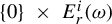 for
$i=1,\ldots ,r(\omega ,x)$
 must appear in
$V_F^j(\omega ,x)$
 for some
$j=1,\ldots ,k(\omega ,x)$
 .
Now, we consider
$(\omega ,x)\in \Delta _0\cap \Delta _1\cap (\Omega _0\, \times \, \mathcal {M})$
 . For any
$\eta \in V_F^{k(\omega ,x)}(\omega ,x)$
 , then
$\eta =(u_\eta ,v_\eta )$
 with respect to the decomposition
$T_{(\omega ,x)}(\Omega \, \times \, \mathcal {M})=T_\omega \Omega \, \times \, \{0\}\oplus \{0\}\, \times \, T_x\mathcal {M}$
 . We claim that
$P(H_\theta ^l(\omega ))u_\eta \not =0$
 . Otherwise, by Lemma 4.1(1), for any
$\eta ^\prime =(u_{\eta ^\prime },v_{\eta ^\prime })$
 with
$P(H_\theta ^l(\omega ))u_{\eta ^\prime }\not =0$
 ,

which contradicts the largest Lyapunov exponents. This argument also implies that
$\lambda _F^{k(\omega ,x)}=\lambda _\theta ^l$
 and
$\dim V_F^{k(\omega ,x)}=\dim H_\theta ^l$
 . Similarly, one can show that

For any
$\xi \in V_F^{1}(\omega ,x)$
 , then
$\xi =(u_\xi ,v_\xi )$
 with respect to the decomposition
$T_{(\omega ,x)}(\Omega \, \times \, \mathcal {M})=T_\omega \Omega \, \times \, \{0\}\oplus \{0\}\, \times \, T_x\mathcal {M}$
 . We claim that
$P(H_\theta ^1(\omega ))u_\xi \not =0$
 . Otherwise, by Lemma 4.1(2), for any
$\xi ^\prime =(u_{\xi ^\prime },v_{\xi ^\prime })$
 with
$P(H_\theta ^1(\omega ))u_{\xi ^\prime }\not =0$
 ,

which contradicts the smallest Lyapunov exponents. This argument also implies that
$\lambda _F^{1}=\lambda _\theta ^1$
 and
$\dim V_F^{1}=\dim H_\theta ^1$
 . Similar, one can show that

By (1.4),
$\lambda _r^i(\omega ,x)$
 for
$i=1,\ldots ,r(\omega )$
 are bounded between
$\lambda _{\theta }^{l_1}=\lambda _{\theta ,\max }^{-} $
 and
$\lambda _\theta ^{l_1+1}=\lambda _{\theta ,\min }^{+}$
 . Therefore, the Lyapunov spectrum of F at
$(\omega ,x)\in \Delta _0\cap \Delta _1\cap (\Omega _0\, \times \, \mathcal {M})$
 is
$\{(\lambda _\theta ^1,\dim H_\theta ^1),\ldots ,(\lambda _\theta ^{l_1}, \dim H_\theta ^{l_1}),$
 $(\lambda _r^1(\omega ,x),\dim E_r^1(\omega ,x)),\ldots ,(\lambda _r^{r(\omega ,x)},\dim E_r^{r(\omega )} (\omega ,x)),(\lambda _\theta ^{l_1+1},\dim H_{\theta }^{l_1+1}(\omega )),\ldots ,(\lambda _\theta ^l,\dim H_\theta ^l(\omega ))\}. $

Using the Abramov–Rohlin formula, we finally prove that

which implies that
$\mu $
 is an SRB measure for
$(\Omega \, \times \, \mathcal {M},F).$

Funding
The first author was partially supported by NSFC (12401230) and the second author was partially supported by NSFC (12501244) and Early-Career Young Scientists and Technologists Project of Jiangxi Province.



