




No CrossRef data available.
UNIFORM ORDER STATISTICS PROPERTY AND [ell ]∞-SPHERICAL DENSITIES
Published online by Cambridge University Press: 01 July 2004
Abstract
In this article, we observe that processes with the uniform order statistics property (UOSP) can be characterized by the condition that their first n epoch times have a joint [ell ]∞≤-spherical density, n ≥ 1. Some related results, and some further properties of [ell ]∞≤-spherical densities, are also given. We also extend some of the results regarding the UOSP to the more general (not necessarily uniform) order statistics property. Finally, we develop a theory of discrete-time discrete-state processes with the UOSP, where the need to consider multiple jumps, at a single time point, arises.
Information
- Type
- Research Article
- Information
- Probability in the Engineering and Informational Sciences , Volume 18 , Issue 3 , July 2004 , pp. 275 - 297
- Copyright
- © 2004 Cambridge University Press
1. INTRODUCTION AND PRELIMINARIES
An n-dimensional density function f of the form

(where

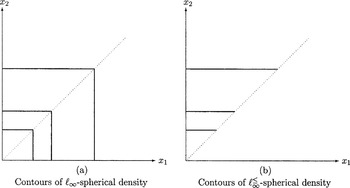
is some function) is called [ell ]∞-spherical. Note that if X1,X2,…,Xn have an [ell ]∞-spherical density, then X1,X2,…,Xn must be exchangeable. Some typical equiprobability contours of a bivariate [ell ]∞-spherical density are depicted in Figure 1a. The density function g of the corresponding order statistics is given by

where

In this article, any density of the form of g in (1.2), for some ψ, will be called [ell ]∞≤-spherical. Note that if X1,X2,…,Xn have an [ell ]∞≤-spherical density, then X1 ≤ X2 ≤ ··· ≤ Xn with probability 1. Some typical equiprobability contours of a bivariate [ell ]∞≤-spherical density are depicted in Figure 1b.

Equiprobability contours.
Remark 1.1: From Figure 1b, it is obvious that if X1 and X2 have a bivariate [ell ]∞≤-spherical density, then the conditional distribution of X1, given that X2 = t (for any t > 0), is uniform(0,t). Similarly, also the conditional distribution of X1, given that X1 ≤ t and X2 > t, is uniform(0,t). Later in this article, it will be shown that these results hold also in the more general multivariate case.
With any set of nonnegative random variables that satisfy X1 ≤ X2 ≤ ··· ≤ Xn with probability 1, we may associate the nonnegative increments

The densities fX and fZ, of X = (X1,X2,…,Xn) and Z = (Z1,Z2,…,Zn), respectively, are related by the equation

It follows that X has an [ell ]∞≤-spherical density if and only if fZ is of the form

for some function φ; densities of this form are called Schur-constant (see Spizzichino [17]). This equivalence is useful for the purpose of identifying random vectors with [ell ]∞≤-spherical densities.
A counting process

is said to be a nonhomogeneous pure birth process with intensity (or rate) functions ri ≥ 0 if


Here and in the following,

may be ∞. Nonhomogeneous pure birth processes have been extensively used recently as a modeling tool in reliability theory and statistics; see, for instance, some references in Shaked, Spizzichino, and Suter [16, pp.275,276]. Also, sequential order statistics, as described in Kamps [13, Sect.1.3], can be easily seen to have the same distribution as the first epoch times of a nonhomogeneous pure birth process.
Shaked et al. [16] showed that if a random vector X = (X1,X2,…, Xn) has an [ell ]∞≤-spherical density function of the form (1.2), then there exists a nonhomogeneous pure birth process whose first n epoch times T1 ≤ T2 ≤ ··· ≤ Tn satisfy

Recall that a process

is called a stationary mixed Poisson process if there exists a unit rate homogeneous Poisson process

and a nonnegative random variable W, independent of K, such that

Grandell [7] provides a detailed coverage of the theory and applications of mixed Poisson processes.
We will also use in the sequel the notion of a mixed uniform sample process. In order to define it, let

and let U1,U2,… be a sequence of independent uniform

random variables. Let L be a positive integer-valued random variable, independent of the Ui's. Given L = l, let

be the empirical distribution function based on U1,U2,…,Ul. The unconditional process

will be called a mixed uniform sample process. Here, and in the rest of the article, “empirical distribution function” means the nonnormalized version of it; that is, if we call

an empirical distribution function, we mean that for every

, the value M(t) is the number of observations in the underlying sample that are less than or equal to t.
We now define the uniform order statistics property (UOSP). We will say that a (finite or infinite) sequence of nonnegative random variables X1 ≤ X2 ≤ ··· has the UOSP if for any k ≥ 1 and for any t > 0 such that P{Xk ≤ t, Xk+1 > t} > 0, the conditional distribution of X1,X2,…,Xk, given that Xk ≤ t and Xk+1 > t, is the joint distribution of k order statistics from a uniform(0,t) distribution. Furthermore, consider a point process

with right-continuous sample paths, such that almost surely M(0) = 0, and M(t) < ∞ for all

. Denote by T1 ≤ T2 ≤ ··· the jump times of the process. The process M is said to have the UOSP if for every

and k ≥ 1 such that P{M(t) = k} > 0, the conditional distribution of T1,T2,…,Tk, given that M(t) = k, is the joint distribution of k order statistics from a uniform(0,t) distribution.
From Remark 1.1 it is seen that if X1 and X2 have a bivariate [ell ]∞≤-spherical density, then they have the UOSP. Later, in Section 2, it will be shown that this is the case also in the more general multivariate case.
The interest of processes with the UOSP was pointed out in Crump [3], where it was shown that they have the Markov property. From Puri [15], it follows that if a process {M(t), t ∈ [0,∞)} (note that here

) has the UOSP, then it has to be a stationary mixed Poisson process. On the other hand, for a finite

, if a process

has the UOSP, then it has to be a mixed uniform sample process. It is worthwhile to note that a mixed sample process on

(here

is finite) might also be a stationary mixed Poisson process. However, in Deffner and Haeusler [4], it is shown that not all mixed sample processes can be represented as stationary mixed Poisson processes.
In the present article, we observe that processes with the UOSP can be characterized by the condition that their first n epoch times have a joint [ell ]∞≤-spherical density, n ≥ 1. Some related results are also given. We also extend some of the results regarding the UOSP to the more general (not necessarily uniform) order statistics property; in particular, we characterize such processes in terms of the joint density of the first n epoch times (for any n). Finally, we develop a theory of discrete-time discrete-state processes with the UOSP, where the need to consider multiple jumps, at a single time point, arises. Because of the need to consider both unit jumps and multiple jumps (at each discrete time point), we are led to study two different notions of discrete UOSP.
Other results that are related to those in the present article can be found in Benczur [1], in a recent paper by Iglesias,

, Pereira, and Tanaka [10], and in references cited therein.
2. CHARACTERIZATIONS OF PROCESSES WITH THE UOSP BY MEANS OF [ell ]∞-SPHERICAL DENSITIES
We start this section with an interesting property of random vectors with [ell ]∞-spherical densities. It will be seen later that this property is closely related to the UOSP of the underlying random variables.
Proposition 2.1: If X1,X2,…,Xn have an [ell ]∞-spherical density f of the form (1.1), then any k-dimensional marginal of f is also an [ell ]∞-spherical density, k ≤ n.
Proof: By the exchangeability of f and backward induction, it suffices to prove that the marginal density fn−1 of (X1,X2,…,Xn−1) is [ell ]∞-spherical. Now, we write

that is, for

, we have that fn−1 is a function of max1≤i≤n−1 xi only. █
In a similar manner, the following result can be obtained.
Proposition 2.2: If X1 ≤ X2 ≤ ··· ≤ Xn have an [ell ]∞≤-spherical density as in (1.2), then so do X1 ≤ X2 ≤ ··· ≤ Xk for any k ≤ n.
Proposition 2.2 leads to the following natural question of “extendibility”: If X1 ≤ X2 ≤ ··· ≤ Xn have an [ell ]∞≤-spherical density as in (1.2), can they be the first n variables of a collection X1 ≤ X2 ≤ ··· ≤ Xn ≤ Xn+1 that have an [ell ]∞≤-spherical density in

? In order to answer this question, denote the joint density of X1 ≤ X2 ≤ ··· ≤ Xn as

and supposing that X1 ≤ X2 ≤ ··· ≤ Xn ≤ Xn+1 also have an [ell ]∞≤-spherical density, denote it by

Obviously,

from which

It follows that X1 ≤ X2 ≤ ··· ≤ Xn is [ell ]∞≤-spherically extendable if and only if ψn is differentiable and nonincreasing.
Regarding the function ψn, it is worthwhile to note that it is related to the density function fXn of Xn; it is easy to verify that

Next, we show that any random vector with an [ell ]∞≤-spherical density has the UOSP, and vice versa.
Proposition 2.3: The random variables X1 ≤ X2 ≤ ··· ≤ Xn have an [ell ]∞≤-spherical density as in (1.2) if and only if they have the UOSP.
Proof: First, suppose that X1 ≤ X2 ≤ ··· ≤ Xn have an [ell ]∞≤-spherical density as in (1.2). Fix a t > 0. By Proposition 2.2, it is seen that it suffices to show that the conditional distribution of X1,X2,…,Xn−1, given that Xn−1 ≤ t and Xn > t, is the joint distribution of n − 1 order statistics from a uniform(0,t) distribution.
Denote by fX1,X2,…,Xn−1|Xn−1≤t,Xn>t the conditional density of X1,X2,…,Xn−1, given that Xn−1 ≤ t and Xn > t. Let 0 ≤ x1 ≤ x2 ≤ ··· ≤ xn−1 ≤ t. Then,

that is, for each t, it is seen that fX1,X2,…,Xn−1|Xn−1≤t,Xn>t(x1,x2,…,xn−1) is constant over the region {(x1,x2,…,xn−1)|0 ≤ x1 ≤ x2 ≤ ··· ≤ xn−1 ≤ t}. In other words, the conditional density fX1,X2,…,Xn−1|Xn−1≤t,Xn>t is the density of n − 1 order statistics from a uniform(0,t) distribution.
Conversely, suppose that X1 ≤ X2 ≤ ··· ≤ Xn have the UOSP. Fix a t > 0. Let 0 ≤ x1 ≤ x2 ≤ ··· ≤ xn−1 ≤ t. Then, on one hand,

and, on the other hand,

that is,

Differentiating (2.2) with respect to t, it is seen that when 0 ≤ x1 ≤ x2 ≤ ··· ≤ xn−1 ≤ t, then f (x1,x2,…,xn−1,t) does not depend on the actual values of x1,x2,…,xn−1. █
A straightforward modification of the proof of Proposition 2.3 yields the following result.
Proposition 2.4: The random variables X1 ≤ X2 ≤ ··· ≤ Xn have an [ell ]∞≤-spherical density as in (1.2) if and only if the conditional distribution of X1,X2,…,Xk, given that Xk+1 = t, is the joint distribution of k order statistics from a uniform(0,t) distribution, for all k ≤ n − 1 and t > 0 for which the above conditional distribution is defined.
From Proposition 2.3 we get the following characterization of processes that have the UOSP property.
Theorem 2.5: A point process

has the UOSP if and only if its first n epoch times T1 ≤ T2 ≤ ··· ≤ Tn have a joint [ell ]∞≤-spherical density for every n ≥ 1 such that P{Tn < ∞} = 1.
We thus see that for a point process N = {N(t), t ∈ [0,∞)}, the following properties are equivalent:
(i) N is a stationary mixed Poisson process.
(ii) N has the UOSP.
(iii) The first n epoch times of N have a joint [ell ]∞≤-spherical density, n ≥ 1.
The equivalence of properties (i) and (ii) has already been known in the literature for a long time (see, for instance, references in Puri [15]). It is worthwhile to mention that in a recent proof of the equivalence of properties (i) and (ii) in Hayakawa [8], the equivalence of the first two conditions with property (iii) is essentially implicit. Namely, in the proof of her Theorem 3.2, Hayakawa [8] obtained the fact that the joint density function of the first n interepoch intervals of N, evaluated at the point (y1,y2,…,yn) ≥ 0, depends only on

; in other words, the density is Schur-constant; see (1.3). As we have mentioned earlier, a sequence of interepoch intervals satisfies the above property if and only if the corresponding first n epoch times have a joint [ell ]∞≤-spherical density, n ≥ 1.
A sequence of positive random variables {Y1,Y2,…,} is called [ell ]1-isotropic (see, for example, Berman [2] or Hayakawa [8]) if and only if for every n ≥ 1, the random variables

are distributed as a set U1,U2,…,Un of independent uniform(0,1) random variables, conditioned on

. From a result of Berman [2] (given as Theorem 2.1 in Hayakawa [8]), it follows that a sequence of positive random variables {Y1,Y2,…} is [ell ]1-isotropic if and only if the joint density function of any finite number of the Yi's is Schur-constant. We can therefore restate Theorem 2.5 as follows.
Theorem 2.6: A point process

has the UOSP if and only if for every n ≥ 1 such that P{Tn < ∞} = 1, the first n epochs times T1 ≤ T2 ≤ ··· ≤ Tn of N satisfy that

are distributed as the order statistics of n − 1 independent uniform(0,1) random variables.
3. SOME COMMENTS ON THE GENERAL OSP
In this section we extend some of the UOSP results in Section 2 to the more general order statistics property (OSP) that will be defined shortly. These extensions entail generalizations of the notions of [ell ]∞-spherical and [ell ]∞≤-spherical densities.
Let a : [0,∞) → [0,∞) be a differentiable, strictly increasing function such that a(0) = 0. This function will be fixed throughout this section. Denote by a−1 the inverse of a, and by a′, its derivative. If X1,X2,…,Xn have the joint density given in (1.1), then

has the density given by

which is a generalization of (1.1). The density function

of the corresponding order statistics is given by

which is a generalization of (1.2).
We now define the order statistics property (OSP), which is a generalization of the UOSP. Let {Ft}t≥0 be a family of distribution functions such that Ft has the support [0,t] . We will say that a (finite or infinite) sequence of nonnegative random variables

has the OSP with respect to {Ft}t≥0 if for any k ≥ 1 and for any t > 0 such that

, the conditional distribution of

, given that

, is the joint distribution of k order statistics based on a sample from Ft. Furthermore, consider a point process

with right-continuous sample paths, such that almost surely

for all

. Denote by

the jump times of the process. The process

is said to have the OSP with respect to {Ft}t≥0 if for every

, such that

, the conditional distribution of

, given that

, is the joint distribution of k order statistics based on a sample from Ft.
Let

be a point process with right-continuous sample paths, such that almost surely

for all t ∈ [0,∞). Denote

, and γ = limt→∞ m(t). From Puri [15] it follows that if the process

has the OSP with respect to some {Ft}t≥0 and γ = ∞, then

has to be a nonstationary mixed Poisson process; that is,

where K is a unit rate homogeneous Poisson process and W is a positive random variable, independent of K. On the other hand, if γ < ∞, then

has to be a mixed sample process with the kernel function

that is,

can be represented as the empirical distribution of a sample of a random size from the above distribution F.
Using the transformation (3.1) or its inverse, it is possible to obtain results about the OSP from results about the UOSP and vice versa. For example, if

have a joint density function

of the form (3.2), then any k-dimensional marginal of

is also of that form, k ≤ n (this statement is a generalization of Proposition 2.1). A generalization of Proposition 2.3 is the following.
Proposition 3.1: The random variables

have a density of the form (3.3) if and only if they have the OSP with respect to {Ft}t≥0, where

From Proposition 3.1 we get the following generalization of Theorem 2.5.
Theorem 3.2: Let a : [0,∞) → [0,∞) be a differentiable, strictly increasing function such that a(0) = 0, and for t ≥ 0, let Ft be defined by (3.4). A point process

has the OSP with respect to {Ft}t≥0 if and only if for every n ≥ 1 such that

, its first n epoch times

have a joint density of the form (3.3).
Example 3.3: The linear birth (Yule) process N = {N(t), t ≥ 0}, with initial population size k, is a nonhomogeneous pure birth process (see (1.4)–(1.6)) with intensity functions

where λ > 0 is some constant. Let T1 ≤ T2 ≤ ··· ≤ Tn be the first n jump times of N. The joint density function of T1,T2,…,Tn, evaluated at x1 ≤ x2 ≤ ··· ≤ xn, can be computed as follows (see, e.g., (2.5) in Shaked et al. [16]; there is there an easily correctable mistake in the indexing):

where x0 ≡ 0. A straightforward algebra yields (for x1 ≤ x2 ≤ ··· ≤ xn)

that is, fT1,T2,…,Tn is of the form (3.3) with

. Now, from Proposition 3.1 it follows that N has the OSP with respect to {Ft}t≥0, where

Applying the inverse of the transformation (3.1), it follows that eλT1 − 1,eλT2 − 1,… have the UOSP. The latter result was obtained in Neuts and Resnick [14] by means of a straightforward, but lengthy, computation.
An interesting application in Bayesian inference in which densities of the form (3.2) arise naturally is described next. Let Θ = (Θ1,Θ2,…,Θn) be a vector of independent and identically distributed positive parameters, and let V (which may be a random variable or a random vector) be an observation whose distribution depends on Θ only through max1≤i≤n Θi; that is, suppose that the joint density of Θ is of the form

where h is some density function on (0,∞), and that the conditional density of V given Θ = (θ1,θ2,…,θn) is of the form

for some function φ. Then, by Bayes' formula, the conditional density of Θ, given V = v, is given by

that is, given V = v, this density is of form (3.2). A particular application in reliability theory is described in the following example.
Example 3.4: Consider r components D1,D2,…,Dr whose lifetimes are denoted by V1,V2,…,Vr, respectively. Suppose that a parallel system of n identical components, with independent lifetimes Θ1,Θ2,…,Θn, supports the performance of D1,D2,…,Dr; that is, suppose that when the supporting parallel system is up, then the failure rate of each Dj is λ0, whereas when the supporting parallel system is down, the failure rate of each Dj is λ1, where λ0 < λ1. Assume that the joint density of Θ1,Θ2,…,Θn is given by (3.5). Then, the conditional density of (Θ1,Θ2,…,Θn), given (V1,V2,…,Vr), is of the form (3.6). It follows from Proposition 3.1 that the conditional distribution of the ordered Θi's, given (V1,V2,…,Vr), has the OSP with respect to {Ft}t≥0, where

(H is the distribution function associated with h).
4. DISCRETE UOSP AND DISCRETE [ell ]∞-SPHERICAL DENSITIES
Inspired by the UOSP for processes with continuous interepoch intervals, Huang and Shoung [9] have introduced a corresponding property for discrete-time point processes (i.e., processes with discrete interepoch intervals and unit step jumps). In this section, we will describe this property and a modification of it that is useful in some applications. We will then derive some discrete analogs of the results in Section 2. It turns out that in the discrete case, it is also of interest to consider processes that can have jumps larger than unity at the jump epochs; thus, we will also obtain further results that have no continuous analogs.
First, we introduce some notation and terminology that are used in this section and point out some simple observations. In this section, we use the notation

for {1,2,…}.
Let Z1,Z2,…,Zn be

-valued random variables and set

Thus, X1,X2,…,Xn are also

-valued and they satisfy

If we denote by pZ and pX the discrete densities of (Z1,Z2,…,Zn) and (X1,X2,…,Xn), respectively, then, obviously,

If, on the other hand, Z1,Z2,…,Zn are

-valued random variables and X1,X2, …,Xn are as defined in (4.1), then X1,X2,…,Xn are also

-valued and they satisfy

In this case, the discrete density functions of (Z1,Z2,…,Zn) and (X1,X2,…,Xn) satisfy

We will say that a discrete joint density p on (

[respectively

] is Schur-constant if

for some function φ, and that it is [ell ]∞-spherical if

for some function φ. A discrete joint density p on

will be called [ell ]∞≤-spherical if

for some function ψ. A discrete joint density p on

will be called [ell ]∞<-spherical if

for some function ψ. Obviously, the above pZ is Schur-constant on

[respectively

] if and only if pX is [ell ]∞≤-spherical [respectively [ell ]∞<-spherical].
The following result is a discrete analog of Proposition 2.1. Its proof is a straightforward modification of the proof of Proposition 2.1 and is therefore omitted.
Proposition 4.1: If the discrete random variables X1,X2,…,Xn have an [ell ]∞-spherical density f on

[respectively

], then any k-dimensional marginal of f is an [ell ]∞-spherical density on

[respectively

], k ≤ n.
We will now define the UOSP for a (finite or infinite) sequence of discrete nonnegative random variables X1,X2,…. Two different definitions are needed depending on whether the Xi's can or cannot be equal to each other. If P{0 < X1 < X2 < ···} = 1, then we say that they have the UOSP (<) if for discrete 0 < x1 < x2 < ··· < xk ≤ t we have

that is, conditional on Xk ≤ t and Xk+1 > t, the random variables X1 < X2 < ··· < Xk are distributed as the order statistics of a sample of size k drawn from the set {1,2,…,t} without replacement. If, on the other hand, P{0 ≤ X1 ≤ X2 ≤ ···} = 1, then we say that these Xi's have the UOSP (≤) if for discrete 0 ≤ x1 ≤ x2 ≤ ··· ≤ xk ≤ t we have

that is, conditional on Xk ≤ t and Xk+1 > t, the random variables X1 ≤ X2 ≤ ··· ≤ Xk are distributed as the order statistics of a sample of size k drawn from the set {0,1,…,t} with replacement. (The latter claim follows from the fact that

is the number of ways that k objects can be put into t + 1 cells; see, e.g., Feller [6, p.38].)
The following result is a discrete analog of Proposition 2.3. Again we omit the proof, as it is a straightforward modification of the proof of Proposition 2.3.
Proposition 4.2: The discrete random variables 0 < X1 < X2 < ··· < Xn [respectively 0 ≤ X1 ≤ X2 ≤ ··· ≤ Xn] have an [ell ]∞<-spherical density as in (4.4) [respectively [ell ]∞≤-spherical density as in (4.3)] if and only if they have the UOSP (<) [respectively UOSP (≤)].
An analog of Proposition 2.4 can also be stated and proven.
In the following, we will now study two kinds of discrete-time discrete-state process: those that have only unit step jumps and those that are more general. We start with discrete-time point processes that have only unit step jumps. Let {A(t), t = 0,1,…} be such a process with A(0) ≡ 0. We assume that P{limt→∞ A(t) = ∞} = 1. The distributional properties of {A(t), t = 0,1,…} can be equivalently described by means of either one of three sequences of random variables:
[bull ] The times of the unit jumps T1,T2,…; that is, Tk = t [hArr ] A(t − 1) = k − 1 and A(t) = k, 1 ≤ k ≤ t (here 0 < T1 < T2 < ··· with probability 1).
[bull ] The interepoch intervals Z1,Z2,…; that is, Zk = Tk − Tk−1, k ≥ 1, where T0 ≡ 0 (here Zk > 0, k ≥ 1, with probability 1).
[bull ] The jump indicators I1,I2,…; that is, It = A(t) − A(t − 1), t ≥ 0.
A process {A(t), t = 0,1,…} as above will be said to have the UOSP (<) if T1,T2,… have this property.
We now recall a definition and a result from Huang and Shoung [9].
Definition 4.3 [9, p.72]: A discrete-time discrete-state process {A(t), t = 0,1,…} is called a mixed geometric process if there exists a random variable Θ that takes on values in (0,1) such that, given that Θ = θ, the interepoch intervals Z1,Z2,… of {A(t), t = 0,1,…} are independent and identically distributed with probabilities Pθ{Zk = z} = θ(1 − θ)z−1, z ≥ 1, k ≥ 1.
Theorem 4.4 [9, p.73]: A discrete-time discrete-state process {A(t), t = 0,1,…} with unit step jumps, such that A(0) = 0 and P{limt→∞ A(t) = ∞} = 1, has the UOSP (<) if and only if it is a mixed geometric process.
We can now obtain the following result; part of it is a discrete analog of Theorem 2.5.
Theorem 4.5: Let {A(t), t = 0,1,…} be a discrete-time discrete-state process with unit step jumps such that A(0) = 0 and P{limt→∞ A(t) = ∞} = 1. The following statements are equivalent:
(i) The process {A(t), t = 0,1,…} has the UOSP (<).
(ii) The process {A(t), t = 0,1,…} is a mixed geometric process.
(iii) The interepoch intervals Z1,Z2,…,Zk have a Schur-constant density on

for every k ≥ 1.
(iv) The epoch times T1,T2,…,Tk have a joint [ell ]∞<-spherical density on

for every k ≥ 1.
(v) The jump indicators I1,I2,…,It are exchangeable for every t ≥ 1.
Proof: The equivalence (i) [hArr ] (ii) is Theorem 4.4. The equivalence (i) [hArr ] (iv) follows from Proposition 4.2. The equivalence (iii) [hArr ] (iv) follows from the comment after (4.4).
(i) ⇒ (v): Fix a t ≥ 1. Let (i1,i2,…,it) ∈ {0,1}t. Suppose that k of the ij's are one and that the other t − k indicators are zero. Then, for some 0 < t1 < t2 < ··· < tk ≤ t, we have

So,

where the second equality follows from the assumption that T1,T2,…,Tk have the UOSP (<); that is, P{I1 = i1,I2 = i2,…,It = it} does not depend on the actual values i1,i2,…,it, but only on the related k. Thus, I1,I2,…,It are exchangeable.
(v) ⇒ (ii): From the de Finetti theorem there exists a probability measure Π on (0,1) such that

for any t ≥ 1, where k is the number of ij's that are one.
Now, fix a k ≥ 1 and a

. Denote

. Then, from (4.5) we get

that is, the process {A(t), t = 0,1,…} is a mixed geometric process. █
The equivalence (ii) [hArr ] (iii) is a well-known de Finetti-type theorem (see, for example, Diaconis and Freedman [5, p.414]). Also, it can be viewed as a discrete analog of Theorem 1.44 in Spizzichino [17].
Using Theorem 4.5, one can obtain interesting discrete Schur-constant, [ell ]∞<-spherical, and exchangeable densities. The following example illustrates this.
Example 4.6: Let Θ in Definition 4.3 have the beta density with parameters α > 0 and β > 0. Then, the Schur-constant joint discrete density of the first k ≥ 1 interepoch intervals is given by

This density (actually the density of (Z1 − 1,Z2 − 1,…,Zk − 1)) is a special case of the beta-compound negative multinomial density (see Johnson, Kotz, and Balakrishnan [11, p.104]); see also Example 4.9. The marginal density of Z1 (which, by exchangeability, is the marginal density of each Zi) is given by

This density (actually the density of Z1 − 1) is a special case of the beta-negative-binomial density, which is also called the Markov–Pólya density; see Johnson, Kotz, and Kemp [12, pp.242,243], but note the different notation; for example, for a > 1, they denote (−a)! = 1/(a − 1)!, and for any nonzero a and b, they denote

, where for a > 0, they use the notation a! = Γ(a + 1).
The [ell ]∞<-spherical joint discrete density of the first k ≥ 1 epoch times is given by

Finally, the exchangeable joint density of the first t ≥ 1 indicators can be computed as follows:

Marginally, each Ij is a Bernoulli random variable with parameter α/(α + β).
In the case when Θ is a uniform(0,1) random variable (i.e., α = β = 1), we have

in particular,

The [ell ]∞<-spherical joint discrete density of the first k ≥ 1 epoch times is then

and the exchangeable density of the first t ≥ 1 indicators is then

Marginally, each Ij is then a Bernoulli random variable with parameter ½.
We now proceed to the study of nondecreasing discrete-time discrete-state processes that can have jumps larger than unity at the jump epochs. These can be described by allowing the interepoch intervals between the “unit jumps” to be equal to zero with a positive probability so that an actual jump of size j > 0 corresponds to a sequence of j consecutive interepoch intervals of size 0. Thus, let {B(t), t = 0,1,…} be such a process (here, we allow jumps at time 0, so we do not require that B(0) = 0 here). The distributional properties of {B(t), t = 0,1,…} can be equivalently described by means of either one of three sequences of random variables:
[bull ] The interepoch intervals between “unit jumps” Z1,Z2,…; that is,

(here, the Zi's can be equal to zero with positive probability).
[bull ] The times of the “unit jumps” T1,T2,…; that is,

(here consecutive Tk's may be equal to each other with positive probability).
[bull ] The jump amounts J0,J1,…; that is, J0 = B(0), and Jt = B(t) − B(t − 1), t ≥ 1 (here, of course, the Jt's can be equal to zero with positive probability and they can also be larger than one).
A process {B(t), t = 0,1,…}, as above, will be said to have the UOSP (≤) if T1,T2,… have this property.
A process {B(t), t = 0,1,…}, as above (i.e., which can have jumps larger than unity), can be a discrete-time discrete-state mixed uniform sample process. In order to define it formally, let

be a positive integer and let U1,U2,… be a sequence of independent random variables distributed uniformly on

. Let L be a positive integer-valued random variable, independent of the Ui's. Given L = l, let

be the empirical distribution function based on U1,U2,…,Ul. The unconditional process

will be called a discrete-time discrete-state mixed uniform sample process. Such processes are useful in studies where the discrete uniform distribution can model some real phenomenon, and a sample, of a size that cannot be predetermined in advance of the experiment, is taken from that distribution.
For processes, as above, that can have general (rather than unit) jumps, we have the following equivalent conditions.
Theorem 4.7: Let {B(t), t = 0,1,…} be a nondecreasing discrete-time discrete-state process. The following statements are equivalent:

Proof: The equivalence (i) [hArr ] (iv) follows from Proposition 4.2. The equivalence (iii) [hArr ] (iv) follows from the comment after (4.4).
(i) ⇒ (ii): The proof of this statement is a modification of the proof of Theorem 4 of Puri [15]. Fix an integer

and set

. From the assumption that {B(t), t = 0,1,…} has the UOSP (≤) it follows that, given L = l, the jump times

are distributed as the order statistics of a sample of size l from a uniform distribution on

; that is,

is an empirical distribution function corresponding to a sample of size l from a uniform distribution on

.
(ii) ⇒ (i): Fix a

and let

. Given L = l, we have that

is an empirical distribution function corresponding to a sample of size l from a uniform distribution on

. Let T1 ≤ T2 ≤ ··· ≤ Tl be the jump points of this empirical distribution (some of the Ti's might be equal to each other if a jump is larger than unity). These Ti's obviously have the UOSP (≤).
(i) ⇒ (v): Fix a t ≥ 0. Let

be a possible realization of (J0,J1,…,Jt). Set

these are the corresponding realized epochs of actual jumps—obviously, there is a finite number k of them. Now we describe the corresponding realization of the epoch times tm's of the zero and nonzero jumps.

Note that above we have described

epoch times tm's; the second equality here follows from the fact that jv's with indices different than αu are all zeros. Let us order these tm's as 0 ≤ t1 ≤ t2 ≤ ··· ≤ tp (note that tp ≤ t). Then,

So,

where the second equality follows from the assumption that T1,T2,…,Tp have the UOSP (≤); that is, P{J0 = j0,J1 = j1,…,Jt = jt} does not depend on the actual values j0,j1,…,jt, but only on

. Thus, J0,J1,…,Jt have a Schur-constant density.
(v) ⇒ (iv): Fix a k ≥ 1 and 0 ≤ t1 ≤ t2 ≤ ··· ≤ tk. Let

that is, tε1 < tε2 < ··· < tεh are the different values in the sequence t1 ≤ t2 ≤ ··· ≤ tk. Obviously, h above is finite (it satisfies h ≤ k). Now, define tk values j0,j1,…,jtk−1 as follows: Let

and let the other tk − h + 1 values jm's be zero. Also, let

that is, a is the number of the last tn's in the sequence t1 ≤ t2 ≤ ··· ≤ tk that are equal to each other. Obviously, 1 ≤ a ≤ k. Then,

Note that

the last equality follows by noting that εh is the index of the (first) largest value in the sequence t1 ≤ t2 ≤ ··· ≤ tk and the number of tn's that are equal to tεh is a. Therefore,

Since (J0,J1,…,Jtk) has a Schur-constant density on (
∪ {0})tk+1, it follows that there exists a function φtk such that

Thus, for a fixed k ≥ 1, when 0 ≤ t1 ≤ t2 ≤ ··· ≤ tk, the probability P{T1 = t1, T2 = t2,…,Tk = tk} depends only on tk; that is, T1,T2,…,Tk have a joint [ell ]∞≤-spherical density on

. █
It is of interest to compare the statement in Theorem 4.5(v) with the one in Theorem 4.7(v). The condition on the jump variables in the former is exchangeability, whereas in the latter, the condition on the jump variables is that they have a Schur-constant density. However, in the setup of Theorem 4.5, these two conditions are the same because for binary random variables, Schur-constant density and exchangeability are equivalent conditions.
It is also of interest to compare the statement in Theorem 4.5(ii) with the one in Theorem 4.7(ii). It is seen that in the discrete-time case, the mixed geometric process is a natural tool for characterizing processes that have unit step jumps and are unbounded, whereas the mixed uniform sample process plays a similar role for characterizing processes that can be bounded and that can have jumps larger than unity.
Remark 4.8: An interesting relationship exists between processes {A(t), t = 0,1,…} such that P{limt→∞ A(t) = ∞} = 1 with the UOSP (<) and processes {B(t), t = 0,1,…} such that P{limt→∞ B(t) = ∞} = 1 with the UOSP (≤). Let Z1,Z2,… be the interepoch intervals of {A(t), t = 0,1,…} as in Theorem 4.5(iii). Define

and let the Zi′'s be the interepoch intervals of a process {B(t), t = 0,1,…} as in Theorem 4.7(iii). If the Z1,Z2,…,Zk have a Schur-constant density on

for each k ≥ 1, then so do Z1′,Z2′,…,Zk′ on

, and vice versa. We thus see that the transformation Zi → Zi′ described above, and its inverse, enable us to go back and forth between processes that have the UOSP (<) and the UOSP (≤), provided they satisfy P{limt→∞ A(t) = ∞} = 1 and P{limt→∞ B(t) = ∞} = 1.
The transformation (4.9) indicates that unbounded processes with unit step jumps (as in Theorem 4.5) that satisfy any of the equivalent conditions in Theorem 4.5 also satisfy a version of the statement in Theorem 4.7(ii). A continuous-time analog of this observation is Theorem 6.6 in Grandell [7].
We will now obtain a relationship among discrete Schur-constant densities that is a discrete analog of (2.1). This will be used in the sequel. Let W1,W2,… be a sequence of random variables taking on values in
, such that the density function of (W1,W2,…,Wn) is of the form (4.2) where the function φ there is denoted here by φn, n = 1,2,…. Then, for any

, we have

that is,

Next, we express the joint density of the jump amounts J0,J1,…,Jt by means of the densities of the interepoch intervals Zi's. For this purpose, let us assume that the density of (Z1,Z2,…,Zn) is of the form (4.2) where the function φ there is denoted here by φn, n = 1,2,…. For t ≥ 0, fix a

and let

, then we have

On the other hand, if p ≥ 1, then

where the first equality follows from the fact that (J0,J1,…,Jt) has a Schur-constant density, the second equality essentially follows from (4.7), and the next to last equality follows from (4.10).
In a similar manner, we can express the joint density of the interepoch intervals Z1,Z2, …,Zk by means of the densities of the jump amounts Ji's. For k ≥ 1, fix a

and let

. If w = 0, then we have

On the other hand, if w ≥ 1, then it can be shown, in a manner similar to the proof of (4.12) (but using (4.8) rather than (4.7)), that

Theorem 4.7 and the transformation (4.9), together with the above observations, enable us to obtain interesting Schur-constant densities on

. The following example illustrates this.
Example 4.9: Let Θ and the Zi's be as in Example 4.6 and let Zi′'s be defined by (4.9). Then, it is a simple matter to see that the Schur-constant density of the first k Zi′'s is given by

This density is a special case of the beta-compound negative multinomial density (see Johnson et al. [11, p.104]).
In order to find the joint density of the first t + 1 ≥ 1 jumps amounts J0,J1,…,Jt, we use (4.12). Fix a

and denote

. If p ≥ 1, then, by (4.12) and (4.13), we have

If p = 0, then, by (4.11), the corresponding probability P{J0 = 0,J1 = 0,…,Jt = 0} is a sum of expressions of the form (4.6).
References
REFERENCES
Benczur, A.
(1968).
On sequences of equivalent events and the compound Poisson process.
Studia Scientiarum Mathematicarum Hungarica
3:
451–458.Google Scholar
Berman, S.M.
(1980).
Stationarity, isotropy and sphericity in
[ell ]p.
Zeitschrift für Wahrscheinlichkeitstheorie und Verwandte
Gebiete
54:
21–23.Google Scholar
Crump, K.S.
(1975).
On point processes having an order statistic structure.
Sankhya A
37:
396–404.Google Scholar
Deffner, A. &
Haeusler, E.
(1985).
A characterization of order statistic point processes that are
mixed Poisson processes and mixed sample processes simultaneously.
Journal of Applied Probability
22:
314–323.Google Scholar
Diaconis, P. &
Freedman, D.
(1987).
A dozen de Finetti-style results in search of a theory.
Annales de L'Institut Henri Poincaré:
Probabilités et Statistiques
23
(Suppl. 2):
397–423.Google Scholar
Feller, W.
(1968).
An introduction to probability theory and its
applications,
Vol. I, 3rd ed.
New York:
Wiley.
Grandell, J.
(1997).
Mixed Poisson processes.
London:
Chapman & Hall.
Hayakawa, Y.
(2000).
A new characterization property of mixed Poisson processes via
Berman's Theorem.
Journal of Applied Probability
37:
261–268.Google Scholar
Huang, W.-J. &
Shoung, J.-M.
(1994).
On a study of some properties of point processes.
Sankhya A
56:
67–76.Google Scholar
Iglesias, Z.P.,
Matús, F.,
Pereira, C.A.B., &
Tanaka, N.I.
(2003).
On finite sequences conditionally uniform given minima and maxima.
Technical Report,
PUC,
Santiago, Chile.
Johnson, N.L.,
Kotz, S., &
Balakrishnan, N.
(1997).
Discrete multivariate distributions.
New York:
Wiley.
Johnson, N.L.,
Kotz, S., &
Kemp, A.W.
(1992).
Univariate discrete distributions,
2nd ed.
New York:
Wiley.
Kamps, U.
(1995).
A concept of generalized order statistics.
Stuttgart:
Teubner.
Neuts, M.F. &
Resnick, S.I.
(1971).
On the times of births in a linear birthprocess.
Journal of the Australian Mathematical Society
12:
473–475.Google Scholar
Puri, P.
(1982).
On the characterization of point processes with the order statistic
property without moment condition.
Journal of Applied Probability
19:
39–51.Google Scholar
Shaked, M.,
Spizzichino, F., &
Suter, F.
(2002).
Nonhomogeneous birth processes and
[ell ]∞-spherical densities, with applications in
reliability theory.
Probability in the Engineering and Informational Sciences
16:
271–288.Google Scholar
Spizzichino, F.
(2001).
Subjective probability models for lifetimes.
London:
Chapman & Hall/CRC.
Equiprobability contours.
 You have
Access
- 6
- Cited by