2.1. Dynamic model of the ship SINS/GNSS system

Following the report by Liang and Jia (Reference Liang and Jia2015), the frame origin at the centroid of the ship, navigation frame, and Earth-centred frame are denoted as b, n and e, respectively. The i frame denotes the Earth-fixed frame, and the $n^{\prime}$ frame denotes the frame computed by SINS relative to the true navigation frame. $C_B^A$ denotes the rotation matrix between A and B. $\omega _{AB}^C$ denotes the rotational rate along C with respect to A or B. Thus, we obtain the nonlinear error model states:

(1)\begin{align}\begin{aligned} \delta \dot{\varOmega } & =(I - C_n^{n^{\prime}})\omega _{in}^n + \delta \omega _{in}^n + C_b^{n^{\prime}}\varepsilon \\ \delta \dot{V} & =[{I - ({C_n^{n^{\prime}}} )} ]C_b^n{{\hat{f}}^b} - ({2\delta \omega_{ie}^n + \delta \omega_{en}^n} )\times ({\hat{V} - \delta V} )+ \delta g + C_b^{n^{\prime}}\nabla \\ \delta \dot{P} & =\delta V + [ - \dot{L},\dot{\lambda }\;\textrm{cos}\,L, - \dot{\lambda }\;\textrm{sin}\;L]\delta P, \end{aligned}\end{align}

where $\delta \dot{\varOmega }$, $\delta \dot{V}$, and $\delta \dot{P}$ denote the component error vectors of attitude, velocity and position, respectively, in the navigation frame, and g represents the gravitational acceleration. $\varepsilon$ and $\nabla$ denote the constant gyroscope bias vector and accelerometer bias vector L and $\lambda$ denote the latitude and longitude of the vehicle, respectively. Moreover, ${f^b}$ and $\omega _{ib}^b$ denote the output of the accelerometer and the gyro in the b frame, respectively. In addition, considering that the speed of the ship is much smaller than the speed of rotation of the Earth, the following equation is obtained (Wen et al., Reference Wen, Yan, Cai and Sun2019):

(2)\begin{align}\begin{aligned} \delta \omega _{ie}^n & =[0, - {\omega _{ie}}\;\textrm{sin}\;\hat{L}\delta L,{\omega _{ie}}\;\textrm{cos}\;\hat{L}\delta L]\\ \delta \omega _{en}^n & =[ - \delta {V_N}/({R_e}(1 - 2e + 3e\;\textrm{sin}\;{L^2}) + \hat{h}),\delta \dot{\lambda }\;\textrm{cos}\;\hat{L} - \lambda \;\textrm{cos}\;\hat{L}\delta L,\\ & \quad \delta \dot{\lambda }\;\textrm{sin}\;\hat{L} + \lambda \;\textrm{cos}\;\hat{L}\delta L]. \end{aligned}\end{align}

where ${R_e}$ is the length if the semimajor axis of the ellipsoid.

The SINS/GNSS integrated system of the surface vessel can then be described as follows:

(3)\begin{align}\begin{aligned} {x_k} & ={\ell _k}({x_{k - 1}}) + {B_k}{\omega _{k - 1}} + {B_f}{f_{k - 1}}\\ {z_k} & ={C_k}{x_{k - 1}} + {D_k}{v_k} + {D_f}{f_k}, \end{aligned}\end{align}

where ${x_k}$ and ${z_k}$ denote the state and measurement vectors in the $k$th epoch, respectively. The noise of SINS ${\omega _k}$ and that of GNSS ${v_k}$ are uncertain and stochastic. When sensor faults exist, the progress and measurement faults are denoted as ${f_{1k}}$ and ${f_{2k}}$, respectively. In addition, ${f_k}\textrm{ = [}{f_{1,k}}\textrm{,}{f_{2,k}}{\textrm{]}^\textrm{T}}$. ${\ell _k}$ is the state transition function.${B_k}$, $C_b^n$ and ${C_k}$ represent known matrices comprising module matrices. ${B_f} = {[{B_k},0]^\textrm{T}}$.${D_k} = {D_f} = {[0,I]^\textrm{T}}$.

2.2 H_i/H_∞ FDF for LDTV system

An LDTV system can be described using the same notations as those in Equation (3):

(4)\begin{align}\begin{aligned} {x_k} & ={F_{l,k}}{x_{k - 1}} + {B_{l,k}}{\omega _{k - 1}} + {B_{lf,k}}{f_{k - 1}}\\ {z_k} & ={C_{l,k}}{x_{k - 1}} + {D_{l,k}}{v_k} + {D_{lf,k}}{f_k} \end{aligned}\end{align}

Here, Equation (4) differs from (3) in that the known ${F_{l,k}}$, ${B_{l,k}}$, ${B_{lf,k}}$ and ${C_{l,k}}$, ${D_{l,k}}$, ${D_{lf,k}}$ are the linearised matrices of input, noise and fault with appropriate dimensions. To detect faults in Equation (4), one can use a residual observer-based FD system, also known as an FDF (Liu et al., Reference Liu, Zhong and Yang2018, Reference Liu, Zhong and Liu2019a), for residual generation, which is an important task of FD. When $({C_{l,k}},{F_{l,k}})$ is detectable and $({F_{l,k}},{B_{l,k}})$ is uniformly stabilisable, the following general residual ${r_k}$ observer-based FDF is proposed:

(5)\begin{align}\left\{\begin{aligned} {{\hat{x}}_k} & ={F_{l,k}}{{\hat{x}}_{k - 1}} + {L_{k - 1}}{{\tilde{y}}_{k - 1}}\\ {{\tilde{y}}_k} & ={z_k} - {C_{l,k}}{{\hat{x}}_k}\\ {r_k} & ={W_k}{{\tilde{y}}_k} \end{aligned}\right.\end{align}

Let ${e_k} = {x_k} - {\hat{x}_k}$. From Equations (4) and (5),

(6)\begin{align}\left\{ \begin{aligned} {e_k} & =({F_{l,k}} - {L_k}{C_{l,k}}){e_{k - 1}} + ({B_{l,k}}{w_k} - {L_k}{D_{l,k}}{v_k})\\& \quad + ({B_{lf,k}} - {L_k}{D_{lf,k}}){f_k}\\ {{\tilde{y}}_k} & ={C_{l,k}}{e_k} + {D_{l,k}}{v_k} + {D_{lf,k}}{f_k}\\ {r_k} & ={W_k}{{\tilde{y}}_k} \end{aligned}\right.\end{align}

where ${L_k}$ is the observer gain matrix of the observation and ${W_k}$ denotes the postfilter matrix.

The transition matrix is defined as ${\phi _{k|i}} = \prod\nolimits_{j = i}^{k - 1} {({F_{l,k|j}} - {L_j}{C_{l,k|j}})}$. Let ${g_{d,k|i}} = {C_{l,k}}{\phi _{k|i + 1}}({B_{l,i}} - {L_k}{D_{l,i}})$ and ${g_{f,k|i}} = {C_{l,k}}{\phi _{k|i + 1}}({B_{l,i}} - {L_k}{D_{lf,i}})$, where ${g_{\varepsilon ,k}} = [{C_k}{\phi _{k|0}},{g_{d,k|0}}, \ldots ,{g_{d,k|k - 1}},{D_{l,k}}]$ and ${g_{\varepsilon f,k}} = [{g_{f,k|0}}, \ldots ,{g_{f,k|k - 1}},{D_{lf,k}}]$. The residual generator then takes the form ${r_k} = {r_{d,k}} + {r_{f,k}}$, ${r_{d, k}} = {W_k}{g_{\varepsilon ,k}}{d_k}$, ${r_{f,k}} = {W_k}{g_{\varepsilon f,k}}{f_k}$.

The following indices are defined considering the robustness of the indices to the unknown noise or inputs and sensitiveness to the faults:

(7)\begin{align}\begin{aligned} ||{{G_{rd}}} ||_{\infty ,[{0,N} ]}^2 & = \mathop {\textrm{sup}}\limits_{f = 0} \dfrac{{\sum\nolimits_{k = 0}^N {{{||{{r_{d,k}}} ||}^2}} }}{{x_0^\textrm{T}\kappa _0^{ - 1}{x_0} + \sum\nolimits_{k = 0}^N {({{{||{{d_k}} ||}^2}} )} }}\\ ||{{G_{rf}}} ||_{\infty ,[{0,N} ]}^2 & = \mathop {\textrm{sup}}\limits_{{x_0},\omega ,v = 0} \dfrac{{\sum\nolimits_{k = 0}^N {{{||{{r_{f,k}}} ||}^2}} }}{{\sum\nolimits_{k = 0}^N {{{||{{f_k}} ||}^2}} }}\\ ||{{G_{rf}}} ||_{ - ,[{0,N} ]}^2 & = \mathop {\textrm{inf}}\limits_{{x_0},\omega ,v = 0} \dfrac{{\sum\nolimits_{k = 0}^N {{{||{{r_{f,k}}} ||}^2}} }}{{\sum\nolimits_{k = 0}^N {{{||{{f_k}} ||}^2}} }} \end{aligned}\end{align}

where ${\kappa _0}\textrm{ = }{x_0}x_0^\textrm{T}\textrm{ = }{P_0}$. $||{{G_{rd}}} ||_{\infty ,[{0,N} ]}^2$ represents the index indicating the robustness of the residual to unknown inputs or acceptable noise. Further, for FD, $||{{G_{rf}}} ||_{\infty ,[{0,N} ]}^2$ and $||{{G_{rf}}} ||_{ - ,[{0,N} ]}^2$ represent the sensitivities of ${r_k}$ toward faults in the best- and worst-case scenarios, respectively.

Thus, the goal of ${r_k}$ is to reduce the unknown input and simultaneously enhance the sensitivity to the faults. Thus, the following maximisation should be satisfied:

(8)\begin{equation}\mathop {\textrm{max}}\limits_{{L_k},{W_k}} \frac{{||{{G_{rf}}} ||_{\infty ,[{0,N} ]}^2}}{{||{{G_{rd}}} ||_{\infty ,[{0,N} ]}^2}}\textrm{ or }\mathop {\textrm{max}}\limits_{{L_k},{W_k}} \frac{{||{{G_{rf}}} ||_{ - ,[{0,N} ]}^2}}{{||{{G_{rd}}} ||_{\infty ,[{0,N} ]}^2}},\end{equation}

which is the so-called H_i/H_∞-FDF (Zhong et al., Reference Zhong, Ding, Zhou and He2020).

Let ${r_{dk}} = \textrm{col}\{{{r_{di}}} \}_{i = 0}^k$, ${r_{fk}} = \textrm{col}\{{{r_{fi}}} \}_{i = 0}^k$. We have ${r_{dk}} = {H_{rd}}{d_k}$ and ${r_{kf}} = {H_{rf}}{f_k}$. ${H_{rd}}$ and ${H_{rf}}$ are as follows:

(9)\begin{align}\begin{aligned} {H_{rd,k}} & = \left[ {\begin{array}{@{}llllll@{}} {{{\bar{g}}_{e,0|0}}}& {{{\bar{D}}_{l,0}}}& 0& \cdots & \cdots & 0\\ {{{\bar{g}}_{e,0|0}}}& {{{\bar{g}}_{d,1|0}}}& {{{\bar{D}}_{l,1}}}& 0& \cdots & 0\\ \vdots & \vdots & \vdots & \ddots & \ddots & 0\\ {{{\bar{g}}_{e,k|0}}}& {{{\bar{g}}_{e,k|0}}}& {{{\bar{g}}_{e,k|1}}}& \cdots & {{{\bar{g}}_{e,k|k - 1}}}& {{{\bar{D}}_{l,k}}} \end{array}} \right]\\ {H_{rf,k}} & = \left[ {\begin{array}{@{}llllll@{}} {{{\bar{D}}_{lf,0}}}& 0& \cdots & \cdots & 0\\ {{{\bar{g}}_{f,1|0}}}& {{{\bar{D}}_{lf,1}}}& 0& \cdots & 0\\ \vdots & \ddots & \ddots & \ddots & 0\\ {{{\bar{g}}_{f,k|0}}}& {{{\bar{g}}_{f,k|1}}}& \cdots & {{{\bar{g}}_{f,k|k - 1}}}& {{{\bar{D}}_{lf,k}}} \end{array}} \right], \end{aligned}\end{align}

where ${\bar{g}_{e,i|0}} = {W_i}{g_{e,i|0}}$, ${\bar{g}_{e,i|j}} = {W_i}{g_{e,i|j}}$, ${\bar{D}_{l,i}} = {W_i}{D_{l,i}}$, and ${\bar{g}_{f,i|j}} = {W_i}{g_{f,i|j}}$, ${\bar{D}_{lf|i}} = {W_i}{D_{lf|i}}$, $i \le k,j \le i - 1$.

Then, we have $||{{G_{rd}}} ||_{\infty ,[{0,N} ]}^2 = {||{{H_{rd,k}}} ||_2}$, $||{{G_{rf}}} ||_{\infty ,[{0,N} ]}^2 = {||{{H_{rf,k}}} ||_2}$, and $||{{G_{rf}}} ||_{ - ,[{0,N} ]}^2 = {||{{H_{rf}}} ||_ - }$.

Based on the above definitions, Equation (8) can be rewritten as

(10)\begin{equation}\mathop {\textrm{max}}\limits_{{L_k},{W_k}} \frac{{{{||{{H_{rf}}} ||}_2}}}{{{{||{{H_{rd}}} ||}_2}}}\textrm{ or }\mathop {\textrm{max}}\limits_{{L_k},{W_k}} \frac{{{{||{{H_{rf}}} ||}_ - }}}{{{{||{{H_{rd}}} ||}_2}}}.\end{equation}

At this juncture, note that $E\{{||{{r_{dk}}} ||} \}\le ||{{H_{rd,k}}} ||\cdot E\{{||{{d_k}} ||} \}$, $E\{{||{{r_{fk}}} ||} \}\le {||{{H_{rf,k}}} ||_2} \cdot E\{{||{{f_k}} ||} \}$ and $E\{{||{{r_{fk}}} ||} \}\ge {||{{H_{rf,k}}} ||_ - } \cdot E\{{||{{f_k}} ||} \}$. Thus, using Equation (4), ${H_i}/{H_\infty }$ can be applied to an FD subject.

With regard to residual evaluation, considering the choice of the threshold, the following assumption is made:

(11)\begin{equation}x_0^\textrm{T}\kappa _0^{ - 1}{x_0} + \sum\limits_{k = 0}^N {({\omega_k^\textrm{T}{\Theta ^{ - 1}}{\omega_k} + v_k^\textrm{T}{\Xi ^{ - 1}}{v_k}} )\le \delta _d^2}\end{equation}

According to this inequality, the error introduced by the estimated initial value ${x_0}$, process noise ${\omega _k}$ and measurement noise ${v_k}$ is less than or equal to the set threshold ${\delta _d}$. $\Theta$, $\Xi$ and ${\kappa _0}$ are weighting matrices determined in the normal case of the above covariance matrix. However, choosing an analytical value of ${\delta _d}$ in real applications is very difficult. Generally, the value is selected based on historical data or experience.

When ${J_N} > {J_{th,0}}$ with an FAR of zero, the ${l_2}[0,N]$ norm-type evaluation ${J_N}$ and threshold ${J_{th,0}}$ with a moderately set sliding window N can be selected as follows:

(12)\begin{align}\begin{aligned} {J_N} & = \dfrac{1}{{N + 1}}\sum\limits_{k = 0}^N {r_k^\textrm{T}{r_k}} \\ {J_{th,0}} & = \dfrac{1}{{N + 1}}||{{G_{rd}}} ||_{\infty ,[{0,N} ]}^2\delta _d^2\end{aligned}\end{align}

3.1 Derivation of the Krein space CKF

To address the nonlinearity in the FD problem using the H_i/H_∞ optimised method from Equation (3), a statistical linearisation approach was adopted.

Consider the nonlinear function of ${\ell _k}$ in Equation (3), evaluated for $i = 1, \ldots 2n$ sampling mapping $(\chi _{k - 1|k - 1}^i,\hat{x}_{k|k - 1}^i)$, where $\chi _{k|k - 1}^i = {\ell _k}({{\chi_{k - 1|k - 1}}} )$, ${\hat{x}_{k|k - 1}} = (1/2n)\sum\nolimits_{i = 1}^{2n} {\chi _{k|k - 1}^i}$ (Julier et al., Reference Julier, Uhlmann and Durrant-Whyte2000). Assuming that the $\hat{x}_{k|k - 1}^i$ can be statistically linearised as ${\hat{x}_{k|k - 1}} = A(\chi _{k - 1|k - 1}^i) + b + \varsigma$, the object can be transformed to obtain $\hat{A}$ and $\hat{b}$ such that the pointwise linearisation error $\varsigma$ is minimised:

(13)\begin{equation}\{{\hat{A},\hat{b}} \}= \arg \min \varsigma {\varsigma ^\textrm{T}}\end{equation}

where $\varsigma = (1/2n)\sum\nolimits_{i = 1}^{2n} {(\hat{x}_{k|k - 1}^i - (A\chi _{k - 1|k - 1}^i + b))}$. Consider the derivatives of objective function with respect to A and b. Taking them to be zero gives the following:

(14)\begin{equation}\begin{array}{l} \hat{b} = \bar{x} - \hat{A}\bar{\chi }\\ \hat{A} = {(P_{k|k - 1}^{x\chi })^\textrm{T}}{(P_{k - 1|k - 1}^{xx})^{ - 1}}, \end{array}\end{equation}

where the parameters are obtained as $\bar{\chi } = (1/2n)\sum\nolimits_{i = 1}^{2n} {\chi _{k - 1|k - 1}^i}$, $\bar{x} = (1/2n)\sum\nolimits_{i = 1}^{2n} {x_{k|k - 1}^i}$; $P_{k - 1|k - 1}^{xx} = (1/2n)\sum\nolimits_{i = 1}^{2n} {(\chi _{k - 1|k - 1}^i - \bar{\chi })} {(\chi _{k - 1|k - 1}^i - \bar{\chi })^\textrm{T}}$; and $P_{k|k - 1}^{x\chi } = (1/2n)\sum\nolimits_{i = 1}^{2n} {(\chi _{k - 1|k - 1}^i - \bar{\chi })} {(\hat{x}_{k|k - 1}^i - \bar{x})^\textrm{T}}$. Then, the estimation error covariance can be calculated as

(15)\begin{align}\begin{aligned} {P_{\varsigma \varsigma }} & =\hat{\varsigma }{{\hat{\varsigma }}^\textrm{T}}\\ & =(1/2n)\sum\limits_{i = 1}^{2n} {(\hat{x}_{k|k - 1}^i - \bar{x} - \hat{A}(\chi _{k - 1|k - 1}^i - \bar{\chi }))\textrm{ }{{(\hat{x}_{k|k - 1}^i - \bar{x} - \hat{A}(\chi _{k - 1|k - 1}^i - \bar{\chi }))}^\textrm{T}}} \\ & =P_{k|k - 1}^{xx} - \hat{A}P_{k - 1|k - 1}^{xx}{{\hat{A}}^\textrm{T}} = P_{k|k - 1}^{xx} - (P_{k|k - 1}^{x\chi }){(P_{k - 1|k - 1}^{xx})^{ - 1}}(P_{k|k - 1}^{x\chi }), \end{aligned}\end{align}

where $P_{k|k - 1}^{xx}$ denotes the covariance of $(\hat{x}_{k|k - 1}^i - \bar{x})$.

Now, considering the exception and the outer product of the statistical linearised model, we obtain the posterior statistics given by

(16)\begin{equation}{x_{k + 1}} = {(P_{k|k - 1}^{x\chi })^\textrm{T}}{(P_{k - 1|k - 1}^{xx})^{ - 1}}({x_k} - {\hat{x}_{k - 1|k - 1}}) + {\hat{x}_{k|k - 1}} + {e_k} + {w_k}.\end{equation}

The linearisation error ${e_k}$, obtained as $E({e_k}e_k^\textrm{T}) = P_{k|k - 1}^{xx} - {(P_{k|k - 1}^{x\chi })^\textrm{T}}{(P_{k - 1|k - 1}^{xx})^{ - 1}}P_{k|k - 1}^{x\chi }$, has a normal Gaussian distribution with zero mean (Zhao and Mili, Reference Zhao and Mili2019).

The same linearisation procedure can be used for the measurement function:

(17)\begin{equation}E({\tau _k}\tau _k^\textrm{T}) = P_{k|k - 1}^{zz} - {(P_{k|k - 1}^{xz})^\textrm{T}}{(P_{k|k - 1}^{xx})^{ - 1}}P_{k|k - 1}^{xz},\end{equation}

where ${\tau _k}$, obtained as $E({\tau _k}\tau _k^\textrm{T}) = P_{k|k - 1}^{zz} - {(P_{k|k - 1}^{xz})^\textrm{T}}{(P_{k|k - 1}^{xx})^{ - 1}}P_{k|k - 1}^{xz}$, has the same properties as ${e_k}$.

Thus, according to Equations (15) and (16), Equation (3) can be transformed as follows:

(18)\begin{align}\begin{aligned} {x_k} & = {F_{l,k}}({x_{k - 1}} - {{\hat{x}}_{k - 1|k - 1}}) + {{\hat{x}}_{k|k - 1}} + {e_k} + {B_{l,k}}{w_k} + {B_{lf,k}}{f_k}\\ {z_k} & = {C_{l,k}}({x_k} - {{\hat{x}}_{k|k - 1}}) + {{\hat{z}}_{k|k - 1}} + {\tau _k} + {D_{l,k}}{v_k} + {D_{lf,k}}{f_k}, \end{aligned}\end{align}

where ${F_{l,k}} = {(P_{k|k - 1}^{x\chi })^\textrm{T}}{(P_{k - 1|k - 1}^{xx})^{ - 1}}$, ${C_{l,k}} = {(P_{k|k - 1}^{xz})^\textrm{T}}{(P_{k|k - 1}^{xx})^{ - 1}}$.

Remark 1: If we move ${F_{l,k}}{\hat{x}_{k - 1|k - 1}}$ and ${\hat{x}_{k|k - 1}}$ to the left-hand side of Equation (18), which is more reasonable in the physical sense, ${C_{l,k}}{\hat{x}_{k|k - 1}}$ and ${\hat{z}_{k|k - 1}}$ are also moved to the left-hand side of the equation. However, this will suppress outlier detection because of data redundancy. For example, if the left side of the observation function is ${z_k} + {C_{l,k}}{\hat{x}_{k|k - 1}} - {\hat{z}_{k|k - 1}}$, the measurement error will be influenced by redundant process noise from the state estimation function and measurement noise as well as by outliers from the observation function, which leads to the equation being affected by noise and faults several times.

3.1.1 Design of a nonlinear H_i/H _∞-FDF

As described in the previous sections, the CKF-integrated navigation system is linearised. Then, to solve the problem of Equation (8), an optimal ${L_k}$ and ${W_k}$ in the observer-based FDF are determined by applying the solution of the linearised H_i/H_∞-FDF in Zhong et al. (Reference Zhong, Ding and Ding2010).

Thus, the following observer-based FDF of the system presented in Equation (18) was considered.

(19)\begin{equation}\begin{array}{l} {{\hat{x}}_k} = {F_{l,k}}{{\hat{x}}_{k - 1}} + {L_{k - 1}}{{\tilde{z}}_{k - 1}} - {F_{l,k}}{{\hat{x}}_{k - 1|k - 1}} + {{\hat{x}}_{k|k - 1}} + {e_k}\\ {{\tilde{z}}_k} = {z_k} - {C_{l,k}}{{\hat{x}}_k}\\ {r_k} = {W_k}{{\tilde{z}}_k}, \end{array}\end{equation}

where the residual function ${J_N}$ and the FD logic are as given in Equation (12).

Next, the following terms are defined: ${\bar{w}_k} = {({Q_k})^{ - 1/2}}{w_k}$, ${\bar{v}_k} = {({R_k})^{ - 1/2}}{v_k}$, and ${s_k} = {x_k} - {\hat{x}_k}$. By subtracting Equation (19) from Equation (18), we obtain the following linearised residual observer function at kth time:

(20)\begin{align}\begin{aligned} {s_{k + 1}} & =({F_{l,k}} - {L_k}{C_{l,k}}){s_k} + {B_{l,k}}{{\bar{w}}_k} - {L_k}{D_{l,k}}{{\bar{v}}_k}\\ & \quad + ({B_{lf,k}} - {L_k}{D_{lf,k}}){f_k}\\ {{\tilde{z}}_k} & ={C_{l,k}}{s_k} + {D_{l,k}}{{\bar{v}}_k} + {D_{lf,k}}{f_k}. \end{aligned}. \end{align}

$({C_{l,k}}, {F_{l,k}})$ and $({F_{l,k}}, {B_{l,k}})$ are uniformly detectable and stabilisable, respectively, in Equation (18). Assuming that the residual covariance in Equation (18) is convergent, the linearisation compensations in ${\bar{w}_k}$ and ${\bar{v}_k}$ are also convergent. Therefore, $E({s_{k + 1}}s_{k + 1}^\textrm{T})$ satisfies the mean square stability.

Considering that Equation (20) is an LDTV system, the solutions of ${L_k}$ and ${W_k}$ presented in Julier et al. (Reference Julier, Uhlmann and Durrant-Whyte2000) can be used to solve Equation (8) approximately as follows:

(21)\begin{align}\begin{aligned} {L_k} & = {F_{l,k}}{P_{k|k - 1}}{({C_{l,k}})^\textrm{T}}R_{\tilde{y},k}^{ - 1}\\ \textrm{ } & = {F_{l,k}}P_{k|k - 1}^{xx}{(P_{k|k - 1}^{zz})^{ - 1}}\\ {R_{\tilde{y},k}} & = {C_{l,k}}{P_{k|k - 1}}{({C_{l,k}})^\textrm{T}} + {D_{l,k}}{R_k}\\ {W_k} & = {({R_{\tilde{y},k}})^{ - 1/2}}\\ {P_{k + 1}} & = (I - {L_k}{C_{l,k}}){P_k}{(I - {L_k}{C_{l,k}})^\textrm{T}} + {D_{l,k}}{R_k}D_{l,k}^\textrm{T} \end{aligned}\end{align}

The proof of optimality for the linear case is presented next.

First, we define $\Phi (i,j) = \prod\nolimits_{k = i}^{j - 1} {({F_{l,k}} - {L_k}{C_{l,k}}),\Phi (i,i) = I}$. Further, Equation (20) can be rewritten as

(22)\begin{align}\begin{aligned} {{\tilde{z}}_k} & =\Omega {s_0} + {\Gamma _w}{{\bar{w}}_N} + {\Gamma _v}{{\bar{v}}_N} + {\Gamma _f}{{\bar{f}}_N}\\ {r_N} & ={W_N}{{\tilde{z}}_N} \end{aligned}\end{align}

where vector ${\upsilon _N}$ denotes ${\textrm{[}\upsilon _0^\textrm{T}\textrm{,}\upsilon _1^\textrm{T} \ldots \upsilon _N^\textrm{T}\textrm{]}^\textrm{T}}$ for an arbitrary vector matrix sequence.

\[\Omega = \left[ {\begin{array}{*{20}{c}} {{C_{l,0}}}\\ {{C_{l,1}}\Phi (1,0)}\\ \vdots \\ {{C_{l,N}}\Phi (N,0)} \end{array}} \right]\]

For ${\Gamma _w}$,

\[\begin{array}{l} {\Gamma _\omega } = {[{\Gamma _\omega }(k,j)]_{(N + 1) \times (N + 1)}}\\ {\Gamma _\omega }(k,k) = 0, \end{array}\]

\[{\Gamma _\omega }(k,j) = \left\{ {\begin{array}{@{}ll} 0& {\textrm{for }k < j}\\ {{C_{l,k}}\Phi (k - 1,j)[{B_{l,k}},0]}& {\textrm{for }k > j} \end{array},} \right.\]

\[{\Gamma _\omega } = {[{\Gamma _\omega }(k,j)]_{(N + 1) \times (N + 1)}}.\]

For ${\Gamma _v}$,

\[{\Gamma _\omega } = {[{\Gamma _\omega }(k,j)]_{(N + 1) \times (N + 1)}},\]

\[{\Gamma _v}(k,k) = {D_{l,k}},\]

\[{\Gamma _v}(k,j) = \left\{ {\begin{array}{*{20}{l}} 0& {\textrm{for }k < j}\\ {{C_{l,k}}\Phi (k - 1,j)[ - {L_k}{D_{l,k}},{D_{l,k}}]}& {\textrm{for }k > j} \end{array}\textrm{ }} \right..\]

For ${\Gamma _f}$,

\[{\Gamma _f} = {[{\Gamma _f}(k,j)]_{(N + 1) \times (N + 1)}},\]

\[{\Gamma _f}(j,k) = {D_{lf,k - 1}},\]

\[{\Gamma _\omega }(k,j) = \left\{ {\begin{array}{*{20}{l}} 0& {\textrm{for }k < j}\\ {{C_{l,k}}\Phi (k - 1,j)[{B_{lf,k - 1}} - {L_{k - 1}}{D_{lf,k - 1}},{D_{lf,j}}]}& {\textrm{for }k > j} \end{array}} \right.\]

Then, one can show that

\begin{align*}||{{G_{rd}}} ||_{\infty ,[{0,N} ]}^2 = ||{{W_N}[\varOmega P_0^{1/2},{\Gamma _w},{\Gamma _v}]} ||_2^2.\end{align*}

When no fault exists, Equation (20) is expressed as follows:

\[\begin{aligned} {s_{k + 1}} & =({F_{l,k}} - {L_k}{C_{l,k}}){s_k} + {B_{l,k}}{{\bar{w}}_k} - {D_{l,k}}{L_k}{{\bar{v}}_k}\\ {{\tilde{z}}_k} & ={C_{l,k}}{s_k} + {D_{l,k}}{{\bar{v}}_k} \end{aligned}\]

where ${s_0}$, ${\bar{w}_k}$ and ${\bar{v}_k}$ are assumed to be zero-mean Gaussian white noise. ${L_k}$, as defined in Equation (21), is the product solution of the well-known gain of KF, i.e., ${K_k}$ and ${F_{l,k}}$ (Zhong et al., Reference Zhong, Ding, Zhou and He2020).

Moreover, the orthogonality of the innovation sequence yields

(23)\begin{align}\begin{aligned} E({{\tilde{z}}_k},\tilde{z}_k^\textrm{T}) & =\textrm{diag}({R_{\tilde{y},0}},{R_{\tilde{y},1}}, \ldots ,{R_{\tilde{y},N}})\\ & = \textrm{[}\Omega \textrm{,}{\Gamma _w}\textrm{,}{\Gamma _v}\textrm{ ]}I{[\Omega \textrm{,}{\Gamma _w}\textrm{,}{\Gamma _v}]^\textrm{T}}\\ & = \Omega {\Omega ^\textrm{T}} + {\Gamma _w}{({\Gamma _w})^\textrm{T}} + {\Gamma _v}{({\Gamma _v})^\textrm{T}}. \end{aligned}\end{align}

Let ${\Lambda _k} = ({F_{l,k}} - {L_k}{C_{l,k}}){P_k}C_{l,k}^\textrm{T} + {\bar{w}_k} - {L_k}{\bar{v}_k}$, considering ${L_k}$ and ${W_k}$. We have ${\Lambda _k} = 0$. When $k \ne j$, all the nondiagonal terms of ${H_{rd,k}}$ in (9) are equal to $\Lambda _k^\textrm{T}{P_k}\Phi _{k,j + 1}^\textrm{T}C_{l,l}^\textrm{T} = 0$.

Then, when ${W_k}$ defined in Equation (21) is applied, we obtain

(24)\begin{align}\begin{aligned} & {W_k}(\Omega {\Omega ^\textrm{T}} + {\Gamma _w}{({\Gamma _w})^\textrm{T}} + {\Gamma _v}{({\Gamma _v})^\textrm{T}})W_k^\textrm{T}\\ & \quad = {W_k}\textrm{(diag}({R_{\tilde{y},0}},{R_{\tilde{y},1}}, \ldots ,{R_{\tilde{y},N}}))W_k^\textrm{T}\\ & \quad = I \end{aligned}. \end{align}

Next, for ${W_k}$ and ${L_k}$, as defined in Equation (21), $||{{G_{rf}}} ||_{\infty ,[{0,N} ]}^2 = I$.

Further, according to Zhong et al. (Reference Zhong, Guo, Guo and Yang2016), ${L_k}$ and ${W_k}$ can be replaced by arbitrary ${L_{ak}}$ and ${W_{ak}}$, for which the FDF remains stable. Thus, there exists a mapping such that the new residual ${r_{aN}}$ can be recovered from the optimal residual ${r_N}$ with ${r_{aN}} = {M_{aN}}{r_N}$, where ${M_{aN}}$ is the mapping matrix.

There exists a mapping (Zhong et al., Reference Zhong, Liu, Zhou, Li and Xue2019) ${\tilde{z}_{ak}} \to {z_{ak}}$such that

(25)\begin{align}\begin{aligned} {\eta _{k + 1}} & =({F_{l,k}} - {L_k}{C_{l,k}}){\eta _k} + ({L_{ak}} - {L_k}){{\tilde{z}}_{ak}}\\ {{\tilde{z}}_k} & ={C_{l,k}}{\eta _k} + {{\tilde{z}}_{ak}}. \end{aligned}\end{align}

The postfilter is set as ${W_k} = {W_{ak}}$, and we obtain

\[{r_{aN}} = {W_{aN}}{\tilde{z}_{aN}} = {W_{aN}}{M_{aN}}{\tilde{z}_N} = {W_{aN}}{M_{aN}}W_N^{ - 1}{r_N},\]

where matrix ${M_{aN}}$ is obtained by replacing ${B_{lf,k}}$, ${D_{lf,j}}$, and ${L_k}$ in ${\Gamma _f}$ with ${L_k}$, I and ${L_{ak}}$, respectively.

Let ${M_{WN}} = {W_{aN}}{M_{aN}}W_N^{ - 1}$. Then, Equation (8) can be rewritten as follows:

\[\begin{aligned} \dfrac{{||{{G_{rf}}} ||_{\infty ,[{0,N} ]}^2}}{{||{{G_{rd}}} ||_{\infty ,[{0,N} ]}^2}}& = \dfrac{{||{{M_{WN}}{G_{rf}}} ||_{\infty ,[{0,N} ]}^2}}{{||{{M_{WN}}{G_{rd}}} ||_{\infty ,[{0,N} ]}^2}}\\ & =\dfrac{{||{{M_{WN}}{G_{rf}}} ||_{\infty ,[{0,N} ]}^2}}{{||{{M_{WN}}} ||_{\infty ,[{0,N} ]}^2}} \le \dfrac{{||{{M_{WN}}} ||_{\infty ,[{0,N} ]}^2||{{G_{rf}}} ||_{\infty ,[{0,N} ]}^2}}{{||{{M_{WN}}} ||_{\infty ,[{0,N} ]}^2}}\\ & = ||{{G_{rf}}} ||_{\infty ,[{0,N} ]}^2 \end{aligned}\]

Alternatively,

\[\begin{aligned} \dfrac{{||{{G_{rf}}} ||_{ - ,[{0,N} ]}^2}}{{||{{G_{rd}}} ||_{\infty ,[{0,N} ]}^2}}& = \dfrac{{||{{M_{WN}}{G_{rf}}} ||_{ - ,[{0,N} ]}^2}}{{||{{M_{WN}}{G_{rd}}} ||_{\infty ,[{0,N} ]}^2}}\\ & =\dfrac{{||{{M_{WN}}{G_{rf}}} ||_{ - ,[{0,N} ]}^2}}{{||{{M_{WN}}} ||_{\infty ,[{0,N} ]}^2}} \le \dfrac{{||{{M_{WN}}} ||_{\infty ,[{0,N} ]}^2||{{G_{rf}}} ||_{ - ,[{0,N} ]}^2}}{{||{{M_{WN}}} ||_{\infty ,[{0,N} ]}^2}}\\ & = ||{{G_{rf}}} ||_{ - ,[{0,N} ]}^2 \end{aligned}\]

Thus, ${W_k}$and ${L_k}$ proposed in Equation (21) provide an optimal solution to Equation (8).

Remark 2: ${P_{k + 1}}$ in Equation (21) is the solution obtained by directly substituting ${L_k}$ into KF covariance based on the framework of the least-squares estimation. When parameters are designed in this manner, the accuracy of state estimation is compromised and the FD performance is improved by ensuring the stability of the filter framework.

Remark 3: Note that a large $||{{G_{rf}}} ||_{\infty ,[{0,N} ]}^2$ does not lead to residual sensitivity to faults. However, we still adopt a large $||{{G_{rf}}} ||_{\infty ,[{0,N} ]}^2$ because it has been widely reported in the literature and because it has the same optimal solution to the H_i/H_∞ problem.

3.2. Randomised analysis of FAR

The choice of ${J_{th,0}}$ in Equation (12) determines the performance of FD. However, a tradeoff between the FAR and fault diagnosis accuracy is required. The smaller the ${J_{th,0}}$, the better is the fault diagnosis accuracy but the poorer is the FAR.

Let us consider the irregular influence of environmental temperature, variation and electromagnetic interference on the inertial measurement unit and the instability of the GNSS signal when ships sail at sea. ${\delta _d}$ in Equation (12) and the probability density function are usually unknown. Thus, a randomised algorithm for probabilistic analysis (Zhong et al., Reference Zhong, Guo, Guo and Yang2016, Reference Zhong, Liu, Zhou, Li and Xue2019) is necessary to estimate the worst-case threshold for generating an acceptable FAR.

As it is difficult to set the value of the threshold ${\delta _d}$ in Equation (12), it can be solved to obtain the sample bounds for estimating the extremum of a random variable as proposed in Chapter 8.4 of Tempo et al. (Reference Tempo, Calafiore and Dabbene2012). First, the number M of the samples in the fault-free case $\textrm{ (}{f_k}\textrm{ = 0)}$ are set and a probabilistic estimate of the worst-case performance is obtained as follows:

(26)\begin{equation}{\hat{J}_N} = \mathop {\max }\limits_i J_N^{(i)}.\end{equation}

In a system without faults, M depends on the number of sampling points. Then, $\alpha$, $\beta$ ${\in} (0,1)$ if the following sample bound is satisfied under the worst-case performance condition:

(27)\begin{equation}M \ge \frac{{\lg \beta }}{{\lg (1 - \alpha )}}.\end{equation}

${\hat{J}_N}$ returns a probabilistic estimation of the threshold generating a given FAR with confidence level $1 - \beta$. The probability ${P_{\textrm{FAR}}}$ of the FD rate is obtained as

(28)\begin{equation}{P_{\textrm{FAR}}} = \Pr \{{{J_N} > {J_{th}}|{f_k} = 0} \}< \alpha\end{equation}

The entire cubature H_i/H_∞-FDF with a given FAR can be obtained as follows:

• Step 1. Set sampling time N, $k = 0$, and set the initial state ${x_0} = 0$.

• Step 2. Calculate ${L_k}$ and ${W_k}$ using Equation (21).

• Step 3. Calculate ${z_{k + 1}}$ using Equation (4).

• Step 4. Update ${\hat{x}_{k + 1}}$ and ${r_{k + 1}}$ using Equation (19).

• Step 5. Reset ${\hat{x}_{k + 1}} = 0$.

• Step 6. Calculate ${J_N}$ using Equation (12).

• Step 7. Choose a threshold using Equation (26), and detect the fault.

• Step 8. $k = k + 1$, return to step 2.

4.1 Description of the simulation scheme

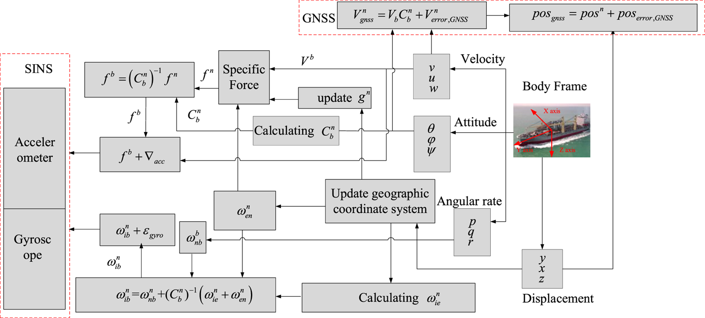
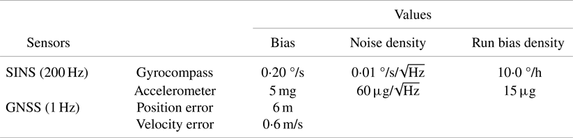
First, to demonstrate the effectiveness of the proposed method, a manoeuvring model group (MMG) model was used whose physical meaning can be clearly interpreted, as proposed by Ogawa and Kasai (Reference Ogawa and Kasai1978). Using this model, sensor data during motion in multiple experiments were generated. The main feature of MMG modelling is that the hydrodynamic forces and moments are clearly decomposed into those acting on the hull, propeller and rudder and those of the interaction among them. Although ship dynamic models have been developed by many scholars (Fossen, Reference Fossen2011; Liang and Jia, Reference Liang and Jia2015), the state estimation accuracy of integrated navigation algorithm is thought to be mainly affected by the initial-state estimation error in the sensor, the system process noise and the measurement noise. This paper proposes an original MMG model that reflects the law of ship motions, which can be refined into a more complex ship dynamic model in future. Based on this classification, the differential equations for velocity, attitude, angular rate and displacement for a vessel's linear and rotation movements around the X-, Y- and Z-axis in the body frame can be solved using Newton's laws. Then, the obtained states are inversed according to the principle of mechanical arrangement and the noise characteristics of the sensors (Table 1). Thus, the simulated sensor data can be obtained, as shown in Figure 1. The interfaces of the simulation system are shown in Figure 2. Because pitching and heaving are not the key considerations for surface merchant vessels, these states were excluded. To avoid accidental conclusions, each experiment was repeated 20 times and the values of simulated sensor noise and the results of integrated navigation were averaged.

Figure 1.

Process of simulation of surface ship sensor data generation

Figure 2.

Interfaces for setting the ship parameters and ship manoeuvring

Table 1.

Detailed parameters of the SINS (MTi-G-710 produced by XSENS)/GNSS generated by the simulator

The process and measurement noises are modelled as first-order Markov process according to the IEEE standards of 2003 and 2016. Second, many factors may cause the failure of the loosely coupled SINS/GNSS integrated navigation system. To summarise, the faults can be divided into hard and soft faults. Hard faults are caused by the sudden faults of measurement output, while soft faults are caused by slow changes due to faults over time.

Hard faults (Zhang et al., Reference Zhang, Zhao, Pang, Wang, Zhang and Feng2020) can be expressed as follows:

(29)\begin{equation}y = \left\{ {\begin{array}{*{20}{c}} {\textrm{count }({t_1} < t < {t_2})}\\ {0\textrm{ }(t \ge {t_2}\textrm{ or }t \le {t_1})} \end{array}} \right.. \end{equation}

Soft faults can be expressed as follows:

(30)\begin{equation}y = k{(t - {t_1})^n} + b, \end{equation}

where t is the time, y is the fault value, k is the fault coefficient, ${t_1}$ and ${t_2}$ are the start and end times of the fault, respectively, and count is the fault information when faults occur.

In the SINS/GNSS system, the main GNSS fault is a short-term outage caused by factors such as interference and signal masking. Thus, for GNSS intermittent faults, we should impose strict requirements for detecting hard faults under different motions. Meanwhile, the SINS on a surface vessel is easily affected by environmental temperature, violent motion variation and electromagnetic interference, which will lead to state divergence as errors accumulate over time. Thus, soft faults mainly affect the performance of SINS.

4.2 Simulation study and discussion

To verify the effectiveness of the proposed FD algorithm, the simulated data in Table 1 and a set of ${l_2}[0,N]$-norm-bounded ${\omega _k}$ and ${v_k}$ were used. Further, $C_b^n\Delta {w_k}$ and $\Delta {v_k}$ were added to the simulated SINS and GNSS noise with a non-Gaussian distribution in a complex environment. Then, the simulated faults were added for various cases.

\[\begin{array}{l} \Delta {w_k} = {[{0.018^ \circ }\textrm{/h},{0.018^ \circ }\textrm{/h},{0.018^ \circ }\textrm{/h},1\mathrm{\ \mu g},1\mathrm{\ \mu g},1\mathrm{\ \mu g}]^\textrm{T}}\sin 2\pi t,\\ \Delta {v_k} = {[0.1,0.1,0.1,1{e^{ - 8}},1{e^{ - 8}},1]^\textrm{T}}\sin 2\pi t. \end{array}\]

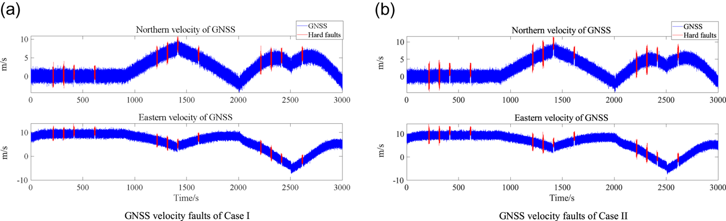
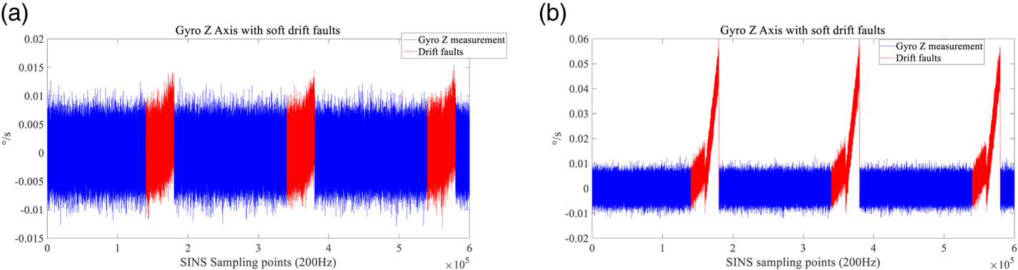
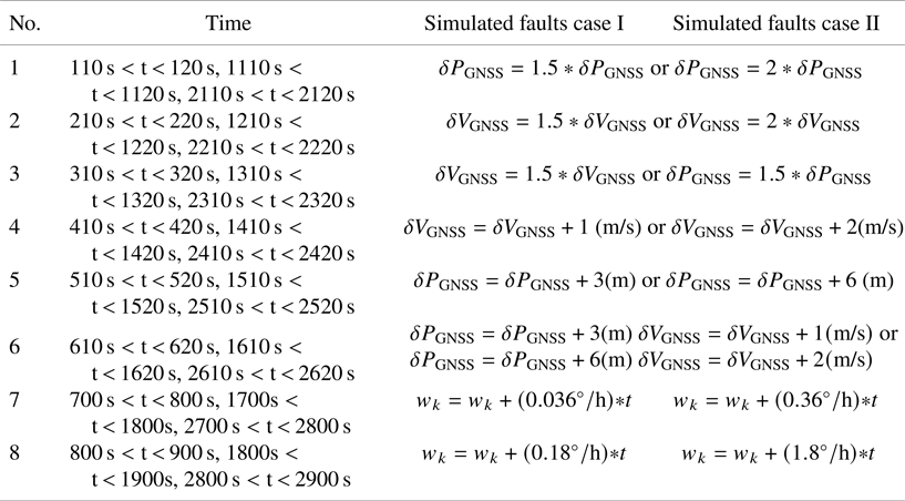
Next, various faults were added when the ship followed different trajectories with different motions (e.g., linear motion and alteration of course and turning) under wind and wave disturbances. Data from a normal navigation simulation were employed. The trajectory and motion state measured using different integrated navigation methods with faults in sensors are shown in Figure 3. The GPS outlier (hard faults) and unexpected inertial sensor drift (soft faults) are considered faults (Table 2). For comparison, the same faults in all three motion modes were added. In addition, the velocity faults of GNSS and the simulated soft drift faults in the Gyro Z-axis of SINS system are shown in Figures 4 and 5.

Figure 3.

Trajectory and motion states of the simulation experiment

Figure 4.

GNSS velocity measurement values after adding hard faults. (a) GNSS velocity faults of case I. (b) GNSS velocity faults of case II

Figure 5.

Simulated soft drift faults in the gyro Z-axis of the SINS system. (a) SINS faults of case I. (b) SINS faults of case II

Table 2.

Simulated hard and soft faults added into the SINS/GNSS system

The trajectory and the motion states are shown in Figure 3. Regardless of whether the system noise and measurement noise are zero-mean Gaussian white noise, the velocity estimation performance of EKF is worse than that of CKF when there are faults in the sensors. With regard to attitude estimation, the difference between the estimation accuracies of EKF and CKF is not obvious when the ship is steady. However, for EKF, with an increasing alteration of the course, the faults cause attitude estimation divergence, especially when the ship turns sharply. (The performance of the case with non-zero-mean Gaussian white noise is worse than that of the case with zero-mean Gaussian white noise.) In other words, although the velocity and position of the GNSS are observable, the EKF can be used to estimate the attitude error in theory to correct the attitude divergence of SINS. However, this correction cannot compensate for the degradation in navigation accuracy caused by sensor faults. An accurate estimation of the velocity and position of the integrated navigation system based on only EKF shows that such a system is considerably dependent on the measurement accuracy of the GNSS. The measurement accuracy of a system based on EKF is worse than that of a system based on CKF when sensor faults are present and when the vessels sailing on the seas perform sharp course alteration or turning manoeuvres.

Next, the threshold is analysed. ${J_N} > \textrm{Threshold}$ implies that the FDF detects the faults. FAR is equal to zero in the fault-free case, and according to Equation (26), we have ${\hat{J}_N} = \mathop {\max }\limits_i J_{N,(\textrm{Cubature})}^{(i)} = \textrm{7}\textrm{.3173}$ and ${\hat{J}_N} = \mathop {\max }\limits_i J_{N,(\textrm{Extended})}^{(i)} = 8.5421$ with a sliding window set with $N = 5$ in Equation (18). However, generally, both the threshold of ${\delta _d}$ in Equation (18) and the probabilistic density function are unknown in practice; hence, the theory in Section 3.2 can be used. Setting the sampling time $M = \textrm{3000}$ in Equation (27), we obtain an acceptable $\textrm{FAR} = 1 - \alpha = 0.999$, from which β is obtained by solving $3000 \ge \lg \beta /(\lg (1 - \alpha ))$. We thus obtain $\beta = 0.0023$. The FAR probability with $\textrm{Threshol}{\textrm{d}_{\textrm{EKF}}} = 7.7941$ and $\textrm{Threshol}{\textrm{d}_{\textrm{CKF}}} = 6.8226$ are less than 0⋅999 with a confidence level of 0⋅9977. The FD results based on extended H_i/H_∞ FDF (Zhong et al., Reference Zhong, Guo, Guo and Yang2016) and cubature H_i/H_∞ FDF are shown in Figures 6 and 7. The circles, boxes and crosses in the figures represent successful detections, false positives and false negatives respectively, excluding SINS soft faults.

Figure 6.

Simulated H_i/H_∞ FDF results of case I faults listed in Table 2. (a) simulated faults with small GNSS error in case I of Table 2. (b) simulated faults with large GNSS error in case I of Table 2

Figure 7.

Simulated H_i/H_∞ FDF results of case II faults in Table 2. (a) Simulated faults with small GNSS error in case II of Table 2. (b) Simulated faults with large GNSS in case II of Table 2

Figure 6 plots the FD results of Case I using the extended H_i/H_∞ FDF and cubature H_i/H_∞ FDF. When the SINS faults were small, neither the extended H_i/H_∞ FDF nor the cubature H_i/H_∞ FDF effectively detected the soft SINS faults of the system [Figure 6(a)] and small GNSS faults are added on the system. The extended H_i/H_∞ FDF and cubature H_i/H_∞ FDF both gave six false negatives, which were mainly position faults with small difference when converted into longitude and latitude. Moreover, the extended H_i/H_∞ FDF was more sensitive to fault responses than the cubature H_i/H_∞ FDF, as reflected in the larger evaluation function threshold value. When larger GNSS faults were added to the GNSS, the evaluation function thresholds of both the extended and cubature H_i/H_∞ FDFs become larger than those in Case I. The extended H_i/H_∞ FDF yielded four false positives and three false negatives, whereas the cubature H_i/H_∞ FDF obtained six false positives and one false negative. Besides being more sensitive to faults, the extended H_i/H_∞ FDF had increased false positive rate. The abovementioned simulation shows that both the methods can effectively detect hard faults of GNSS, but are not sufficiently sensitive to soft, low-magnitude faults of SINS.

Figure 7 shows the simulation results in the case of larger SINS faults. The detection results of hard faults were similar to those in case I. Soft faults occurred between 700 and 900 s, 1,700 and 1,900,s, and 2,700 and 2,900s. After the soft faults disappear, the detection results of the extended H_i/H_∞ FDF included many false alarms, especially in the linear motion stage during 700s~900 s. In the turning phase, however, the number of FD false negatives based on extended H_i/H_∞ FDF has decreased. The cubature H_i/H_∞ FDF converged at faster speed and gave fewer false alarms after the end of soft faults than the extended H_i/H_∞ FDF and completed the detection of hard faults. These results confirm the effectiveness of the proposed algorithm.

When the soft drift faults of SINS are too small, they cannot be detected by the H_i/H_∞ FDF algorithm in every motion stage. The integrated navigation algorithm based on CKF achieves high state estimation accuracy. However, when a soft fault occurs, the amplitude of the ${J_N}$ change is not obvious. However, the error covariance of the state changes significantly (Figure 8). This behaviour will be studied in the authors’ future work. The FD relies not only on the observations but also on the attitude covariance in ${P_k}$ of Equation (21) to determine the presence of soft drift faults.

Figure 8.

Simulated state estimation covariance with small GNSS faults in case I. (a) Simulated velocity estimation covariance with small GNSS faults in case I. (b) Simulated attitude estimation covariance with small GNSS faults in case I