1 Introduction
It is now increasingly common to use computers to perform simulations to check various claims or to predict phenomena of interest. In some sense, numerical simulation has become the ‘third way’ of science, alongside theory and experiment: more and more scientists are checking the correctness, relevance or validity of their claims via numerical simulations (complementing or replacing experiments); in turn, many theories owe their origin to intriguing results obtained via numerical simulation. The fact that numerical simulations have essentially become numerical experiments is made clear in expressions such as ‘in silico experiments’ or the ‘computational microscope’ (Lee et al. Reference Lee, Hsin, Sotomayor, Comellas and Schulten2009).
Numerical experiments are particularly relevant to atomistic systems, which may be very difficult to understand with standard, macroscopic experimental devices in usual conditions of temperature, pressure, etc. For such atomistic systems, molecular simulation is now a recognized approach. For example, two Nobel Prizes in Chemistry have been awarded to pioneers of these methods: in 1998 the prize was awarded to Walter Kohn ‘for his development of the density-functional theory’ and John A. Pople ‘for his development of computational methods in quantum chemistry’, and in 2013 the prize was shared between Martin Karplus, Michael Levitt and Arieh Warshel ‘for the development of multiscale models for complex chemical systems’.
In this introductory section, we first give a general presentation of molecular dynamics, which aims at simulating atomistic systems (see Section 1.1). In particular, we give a brief account of the fundamental concepts of statistical physics that are required in order to understand the models at hand. We next present in Section 1.2 the numerical challenges raised by molecular dynamics, with an emphasis on problems involving partial differential equations (PDEs). It may in fact be unclear to the reader why PDEs should come into the picture. We devote Section 1.3 to explaining why and where tools from the analysis of PDEs can be used to improve the numerical methods used for molecular simulation. The general outline of this article is given at the end of Section 1.3.
1.1 Molecular dynamics simulations
In statistical physics, matter is described at the atomic level in a classical or a quantum setting. There is a wide variety of models with various resolutions, ranging from quantum approaches to computing electronic structures, with methods such as density functional theory and its various implementations (Hohenberg and Kohn Reference Hohenberg and Kohn1964, Kohn and Sham Reference Kohn and Sham1965, Lieb Reference Lieb1983, Cancès et al. Reference Cancès, Defranceschi, Kutzelnigg, Le Bris, Maday, Ciarlet and Le Bris2003), to more coarse-grained descriptions, such as those considered in kinetic Monte Carlo (see for instance the review by Voter Reference Voter, Sickafus, Kotomin and Uberuaga2007) or dissipative particle dynamics (Hoogerbrugge and Koelman Reference Hoogerbrugge and Koelman1992, Español and Warren Reference Español and Warren1995). Among these models, molecular dynamics based on empirical interaction potentials offers an interesting compromise between modelling at the atomistic level and computational cost. On the one hand, quantum approaches are indeed plagued by their high computational cost, although some promising improvements have been made towards the computation of interaction forces scaling linearly with the system size (mostly for insulators, the efficient simulation of metals remaining a challenge). On the other hand, more mesoscopic approaches, such as kinetic Monte Carlo or dissipative particle dynamics, are more difficult to parametrize, and typically provide only qualitative results in some specific physical regimes.
Within molecular dynamics, many computational models also co-exist. Some researchers prefer to use purely deterministic dynamics such as Hamiltonian dynamics or Nosé–Hoover-like dynamics (Nosé Reference Nosé1984b, Nosé Reference Nosé1984a, Hoover Reference Hoover1985, Bond and Leimkuhler Reference Bond and Leimkuhler2007), while others resort to Monte Carlo approaches such as the Metropolis algorithm and its variants (Metropolis et al. Reference Metropolis, Rosenbluth, Rosenbluth, Teller and Teller1953, Hastings Reference Hastings1970). In this review we focus on yet another category of models, which are quite popular: continuous stochastic dynamics, the most famous examples of which are Langevin dynamics and its overdamped limit. The distinction between stochastic and deterministic dynamics is not so clear-cut in many cases. Indeed, deterministic dynamics are sometimes weakly perturbed by a stochastic term, as in the Langevin–Nosé–Hoover method (Leimkuhler, Noorizadeh and Theil Reference Leimkuhler, Noorizadeh and Theil2009). Moreover, there are stochastic dynamics such as Metropolis-like algorithms which are based on deterministic proposals, as in hybrid Monte Carlo approaches (Duane, Kennedy, Pendleton and Roweth Reference Duane, Kennedy, Pendleton and Roweth1987).
1.1.1 Microscopic description of physical systems
To present the dynamics we consider in this review more precisely, we first give a
microscopic description of physical systems. The state of a system composed of  $N$ particles (typically atoms) is completely determined by the
positions
 $q=(q_{1},\ldots ,q_{N})$ and the momenta
 $p=(p_{1},\ldots ,p_{N})$ of all the particles. Recall that, in Cartesian coordinates,
momenta are velocities multiplied by the masses of the particles under
consideration.
One of the fundamental issues in statistical physics is that  $N$ should a priori be of the order of
the Avogadro number to determine the macroscopic behaviour of matter, while, in
practice, current simulations are mostly performed for systems of
 $N=10^{6}-10^{9}$ particles, with heroic computations involving record numbers of
particles of order
 $N=10^{12}$. The systems computed are therefore much smaller, by several
orders of magnitude, than the macroscopic systems they represent. Nonetheless, it
turns out that molecular simulation is often able to give relevant predictions for
the simulated systems. For the simplest systems, such as noble gases, bulk
properties can in fact be estimated with only a few thousand particles.
Momenta take values in  $\mathbb{R}^{3N}$ for three-dimensional systems, whereas positions take values in
a position space
 ${\mathcal{D}}$, which can be either unbounded (the typical case being
 ${\mathcal{D}}=\mathbb{R}^{3N}$ for isolated systems in three dimensions) or bounded (the
typical case being simulations performed in a periodic cell
 ${\mathcal{D}}=(L\mathbb{T})^{3N}$, with
 $\mathbb{T}=\mathbb{R}/\mathbb{Z}$ denoting the one-dimensional torus). The latter situation is
encountered, for example, in the simulation of condensed matter systems, for which
periodic boundary conditions are used to mimic bulk conditions. In this paper we
denote the dimension of the system by
 $d$ (
 $d=3N$ for particles in three-dimensional space), and the phase space
by
 ${\mathcal{E}}={\mathcal{D}}\times \mathbb{R}^{d}$. Since some dynamics only involve the positions while other
dynamics involve both positions and momenta, we will often use the abstract
notation
 ${\mathcal{X}}$ to denote a state space which can be either
 ${\mathcal{D}}$ or
 ${\mathcal{E}}$, depending on context.
The physical content of the model is essentially encoded in the potential energy
function  $V(q)$ that gives the interaction energy of the
 $N$ particles with positions
 $q$. Interaction potentials should ideally be obtained from quantum
mechanical computations based on an approximate numerical solution of the
Schrödinger equation, for fixed nuclei positions (Cancès
et al. Reference Cancès, Defranceschi, Kutzelnigg, Le Bris, Maday, Ciarlet and Le Bris2003, Le Bris Reference Le Bris2005). In practice, as already hinted at above, this is very
expensive, so empirical potentials are often used for large-scale simulations. The
construction and validation of appropriate empirical energy functions is a
research domain in its own right. For some simple systems, satisfactory empirical
potentials are available. This is the case for noble gases such as argon, for
which the potential energy can be written as the sum of pairwise interactions of
Lennard-Jones type. For molecules, two types of interaction should be
distinguished: (i) bonded interactions to model covalent bonds, and
which involve terms depending on bond lengths between two atoms, bending angles
defined using three atoms, and dihedral angles computed using four atoms;
(ii) non-bonded interactions, involving for instance Coulomb
interactions between charged atoms, and Lennard-Jones interactions describing
dipole–dipole interactions (see
e.g. Schlick Reference Schlick2002). For solids, the current trend is towards variations and extensions
of the embedded-atom model proposed in Baskes (Reference Baskes1992), or bond-order potentials such as REBO (Tersoff Reference Tersoff1989) or ReaxFF (van Duin
et al. Reference van Duin, Dasgupta, Lorant and Goddard2001). The latter potentials involve terms
depending on the local environment of the atoms, which allows them to account for
chemical reactions (i.e. bond breakings and bond
formations). For biological applications, a lot of effort is devoted to obtaining
good water models, because of the importance of water as a solvent. Potential
energy functions are implemented in popular molecular dynamics packages such as
AMBER, CHARMM, GROMACS, LAMMPS and NAMD.
The total energy of microscopic systems is given by the Hamiltonian  $H(q,p)$, which is typically the sum of the kinetic energy and the
potential energy,
 $$\begin{eqnarray}H(q,p)=\frac{1}{2}p^{T}M^{-1}p+V(q),\end{eqnarray}$$
where we introduce the mass matrix  $M=\text{diag}(m_{1}\text{Id}_{3},\ldots ,m_{N}\text{Id}_{3})$, assuming that the system is three-dimensional, and
 $m_{i}$ denotes the mass of the
 $i$th particle. Let us also emphasize here that for simplicity we
always consider the potential
 $V$ to be
 $C^{\infty }$ in this review.
Using the potential  $V$, two physical models of the system can be obtained: a model of
the system at equilibrium via thermodynamic ensembles, and a model for the
evolution of the system using appropriate dynamics.
1.1.2 Macroscopic description via thermodynamic ensembles
The macroscopic state of a system at equilibrium is described, within the framework of statistical physics, by a probability measure on the configuration space, called the thermodynamic ensemble. The macroscopic features of the system are then computed as averages of an observable with respect to this measure.
We focus here on the canonical ensemble, in which the number of particles, the domain and the temperature are fixed. Mathematically, it is defined as the minimizer of Boltzmann’s entropy function under the constraint that the average energy is fixed. The Lagrange multiplier associated with this constraint is the temperature. See Balian (Reference Balian2007) for more physical background, as well as Lelièvre, Rousset and Stoltz (Reference Lelièvre, Rousset and Stoltz2010, Section 1.2.3) for a short, self-contained presentation.
For systems described by their positions and momenta, the canonical measure reads
 $$\begin{eqnarray}{\it\mu}(\text{d}q\,\text{d}p)=Z_{{\it\mu}}^{-1}\,\text{e}^{-{\it\beta}H(q,p)}\text{d}q\,\text{d}p,\quad Z_{{\it\mu}}=\int _{{\mathcal{E}}}\,\text{e}^{-{\it\beta}H},\end{eqnarray}$$
where  $H$ is defined by (1.1),
 ${\it\beta}=(k_{B}T)^{-1}>0$ is the inverse temperature, and the normalization constant
 $Z_{{\it\mu}}$ is assumed to be finite. The probability measure
 ${\it\mu}$ is also known as the Boltzmann–Gibbs distribution
associated with the function
 $H$. Note that the components of the momenta are independent under
the canonical measure, and follow a Gaussian distribution.
The macroscopic properties are obtained as averages of functions (called
observables) of the microstate  $(q,p)$ of the system with respect to the canonical measure. For a given
observable
 ${\it\varphi}(q,p)$, macroscopic properties are therefore obtained by computing
 $$\begin{eqnarray}\mathbb{E}_{{\it\mu}}({\it\varphi})=\int _{{\mathcal{E}}}{\it\varphi}(q,p)\,{\it\mu}(\text{d}q\,\text{d}p).\end{eqnarray}$$
In many cases of interest, the integration with respect to the
momenta can be performed analytically (see for instance (1.6) below), or the observable of
interest only depends on the positions  $q$ (as is the case for the potential energy, for instance). The
integral (1.3) then simplifies to
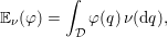 $$\begin{eqnarray}\mathbb{E}_{{\it\nu}}({\it\varphi})=\int _{{\mathcal{D}}}{\it\varphi}(q)\,{\it\nu}(\text{d}q),\end{eqnarray}$$
where  ${\it\nu}$ is the marginal law of
 ${\it\mu}$ in
 $q$:
 $$\begin{eqnarray}{\it\nu}(\text{d}q)=Z_{{\it\nu}}^{-1}\,\text{e}^{-{\it\beta}V(q)}\,\text{d}q,\quad Z_{{\it\nu}}=\int _{{\mathcal{D}}}\,\text{e}^{-{\it\beta}V}.\end{eqnarray}$$
The probability measure  ${\it\nu}$ is the Boltzmann–Gibbs distribution associated with
the function
 $V$. Averages such as (1.3) and (1.4) are called
thermodynamic quantities. As highlighted in the next example and further discussed
in Section 1.2, the actual
challenge to the numerical evaluation of macroscopic properties is generating
positions distributed according to
 ${\it\nu}$ using an appropriate numerical method (see
Sections 3 and 4).
For concreteness, let us give one example: in three-dimensional condensed matter systems equipped with periodic boundary conditions, the pressure is obtained by computing (1.3) with
 $$\begin{eqnarray}{\it\varphi}(q,p)=\frac{1}{3|{\mathcal{D}}|}\mathop{\sum }_{i=1}^{N}\biggl(\frac{|p_{i}|^{2}}{m_{i}}-q_{i}\cdot \frac{\partial V}{\partial q_{i}}(q)\biggr).\end{eqnarray}$$
The contribution of the momenta can be integrated out analytically
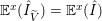
(corresponding to the ideal gas contribution to the pressure), so that  $\mathbb{E}_{{\it\mu}}({\it\varphi})=\mathbb{E}_{{\it\nu}}(\overline{{\it\varphi}})$ where
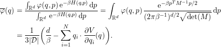 $$\begin{eqnarray}\displaystyle \overline{{\it\varphi}}(q) & = & \displaystyle \frac{\int _{\mathbb{R}^{d}}{\it\varphi}(q,p)\,\text{e}^{-{\it\beta}H(q,p)}\,\text{d}p}{\int _{\mathbb{R}^{d}}\,\text{e}^{-{\it\beta}H(q,p)}\,\text{d}p}=\int _{\mathbb{R}^{d}}{\it\varphi}(q,p)\,\frac{\text{e}^{-{\it\beta}p^{T}M^{-1}p/2}}{(2{\it\pi}{\it\beta}^{-1})^{d/2}\sqrt{\text{det}(M)}}\,\text{d}p\nonumber\\ \displaystyle & = & \displaystyle \frac{1}{3|{\mathcal{D}}|}\biggl(\frac{d}{{\it\beta}}-\mathop{\sum }_{i=1}^{N}q_{i}\cdot \frac{\partial V}{\partial q_{i}}(q)\biggr).\end{eqnarray}$$
1.1.3 Microscopic dynamics
Once a description of the system is provided in terms of degrees of freedom, boundary conditions and potential energy function, we can also discuss its time evolution. For isolated systems, namely in situations where it is possible to simulate the system and its entire environment, systems should evolve according to Hamiltonian dynamics. However, for systems evolving in an environment so large that it fixes the temperature, for example, it is not generally possible to simulate both the system of interest and the ambient environment, which acts as a thermal bath. In this case, a pragmatic approach is to replace the average effect of the environment by some fluctuation/dissipation process which indeed makes the dynamics ergodic with respect to the canonical measure (ergodicity will be discussed in detail below). One theoretical underpinning for this approach is provided by the Mori–Zwanzig framework (Mori Reference Mori1965, Zwanzig Reference Zwanzig1973, Givon, Kupferman and Stuart Reference Givon, Kupferman and Stuart2004). In such cases, the physical relevance of the dynamics considered in molecular dynamics is debatable if one is precisely interested in dynamical properties. We will not discuss this modelling problem further, and focus on two dynamics which are widely used in the community: the Langevin dynamics and its overdamped limit.
Two situations should be distinguished. In some cases, dynamics are used as sampling devices. The focus is then on invariant measures or stationary properties rather than on dynamical information. The aim is to construct dynamics which are ergodic, in the sense that average properties computed along a typical realization converge in the long-time limit to averages with respect to some given measure of interest such as the canonical measure (1.2) (see equation (1.10) below). However, it is also often the case that dynamical properties (which really depend on the dynamics at hand and not only on the measure for which the dynamics is ergodic) are computed. These properties take the general form
 $$\begin{eqnarray}\mathbb{E}[{\it\varphi}((x_{t})_{t\in I})],\end{eqnarray}$$
where  $(x_{t})_{t\in I}$ is a random trajectory over a time interval
 $I$ (which can be finite or infinite), and
 ${\it\varphi}$ is a path functional. In fact, many current numerical challenges
concern the computation of such dynamical properties.
The two paradigmatic dynamics we consider in this work are the following stochastic differential equations (SDEs).
(1) Overdamped Langevin dynamics:
(1.8)where $$\begin{eqnarray}\text{d}q_{t}=-{\rm\nabla}V(q_{t})\,\text{d}t+\sqrt{\frac{2}{{\it\beta}}}\,\text{d}W_{t},\end{eqnarray}$$$W_{t}$ is a standard $d$-dimensional Brownian motion.
(2) Langevin dynamics:
(1.9)where$$\begin{eqnarray}\left\{\begin{array}{@{}l@{}}\displaystyle \text{d}q_{t}=M^{-1}p_{t}\,\text{d}t,\\ \displaystyle \text{d}p_{t}=-{\rm\nabla}V(q_{t})\,\text{d}t-{\it\gamma}\,M^{-1}p_{t}\,\text{d}t+\sqrt{\frac{2{\it\gamma}}{{\it\beta}}}\,\text{d}W_{t},\end{array}\right.\end{eqnarray}$$${\it\gamma}>0$ is a positive parameter.





As discussed in Lelièvre et al. (Reference Lelièvre, Rousset and Stoltz2010, Section 2.2.4), overdamped
Langevin dynamics can be obtained from Langevin dynamics by two limiting processes
when the mass matrix is proportional to the identity matrix ( $M=m\,\text{Id}$): (i) a large friction limit
 ${\it\gamma}\rightarrow +\infty$ with time rescaled as
 ${\it\gamma}t$; (ii) a small mass limit
 $m\rightarrow 0$.
There exist many variations and extensions to the Langevin dynamics, such as
Langevin dynamics with position-dependent friction  ${\it\gamma}(q_{t})$ in (1.9),
dissipative particle dynamics, where the friction depends on the relative
velocities between the particles (Hoogerbrugge and Koelman Reference Hoogerbrugge and Koelman1992, Español and Warren Reference Español and Warren1995), generalized Langevin dynamics, with an extra variable
which can be seen as an integral of the fluctuation/dissipation (Zwanzig Reference Zwanzig1973), and
Langevin–Nosé–Hoover (Leimkuhler
et al. Reference Leimkuhler, Noorizadeh and Theil2009). We restrict ourselves to the
paradigms (1.8) and (1.9) for simplicity. Many numerical
techniques can be extended, at least formally, to other dynamics, although
mathematical proofs of convergence or consistency may be much more complicated,
since the basic ergodic properties of these dynamics may not be known. This is the
case, for example, for the dissipative particle dynamics, for which ergodicity is
proved only in one dimension (Shardlow and Yan Reference Shardlow and Yan2006).
1.2 Numerical challenges in molecular dynamics
Molecular dynamics raises a number of computational challenges. In this article we
mainly focus on sampling problems. Sampling consists in approximating an average by
using empirical averages over a collection of samples, namely realizations of the
underlying random variable distributed according to a target probability measure. We
consider here either thermodynamic quantities, such as (1.3)–(1.4) (in which case the target probability is  ${\it\mu}$ or
 ${\it\nu}$), or dynamical ones, such as (1.7) (in which case the target probability is the law of the
process
 $(x_{t})_{t\in I}$ over the path space). For completeness, we also mention other
challenges in molecular dynamics at the end of this section.
1.2.1 Static sampling problems
Thermodynamic averages such as (1.3) and (1.4) are in general very difficult to approximate by direct numerical integration since the number of particles is very large (and thus the dimension of the space over which the integral is posed is large). This is why stochastic approaches are typically used. The fundamental idea of these methods is to replace ensemble averages with time averages along trajectories of well-chosen dynamics, which are ergodic with respect to the target probability measure. More precisely, when the target measure is the canonical measure (1.2), these dynamics should be such that
 $$\begin{eqnarray}\lim _{t\rightarrow \infty }\frac{1}{t}\int _{0}^{t}{\it\varphi}(q_{s},p_{s})\,\text{d}s=\int _{{\mathcal{E}}}{\it\varphi}(q,p){\it\mu}(\text{d}q\,\text{d}p).\end{eqnarray}$$
Ergodicity means that time averages over trajectories almost
surely converge to a well-defined limit (for  ${\it\mu}$-almost all initial conditions, for almost every realization of
the noise used in the dynamics), this limit being an average over the phase space
with respect to a probability measure (the canonical measure in our context).
Examples of such ergodic dynamics include overdamped Langevin dynamics (1.8) (which is ergodic with respect
to
 ${\it\nu}$) and Langevin dynamics (1.9) (which is ergodic with respect to
 ${\it\mu}$). We will present examples of efficient techniques to compute
thermodynamic quantities in Section 3, the particular case of the computation of free energy differences being
covered in Section 4.
1.2.2 Sampling dynamical properties
Other quantities of interest actually depend on the dynamics. This includes, for
example, time correlation functions (see Section 5) or transition times and paths between regions of the
configuration space (see Section 6). As an example, let us consider an exit problem, which consists in
sampling the random variables  $({\it\tau},(q_{{\it\tau}},p_{{\it\tau}}))$ where
 $$\begin{eqnarray}{\it\tau}=\inf \{t>0,\,q_{t}\not \in A\}.\end{eqnarray}$$
Here  $A$ is a given region of the configuration space (an open bounded
simply connected subset of
 $\mathbb{R}^{d}$), and it is implicitly assumed that
 $q_{0}\in A$. The random variables
 $({\it\tau},(q_{{\it\tau}},p_{{\it\tau}}))$ fully characterize the exit event from
 $A$: they give the exit times and exit points from
 $A$. Sampling the random variables
 $({\it\tau},(q_{{\it\tau}},p_{{\it\tau}}))$ requires us to sample the paths
 $(q_{t},p_{t})_{0\leqslant t\leqslant {\it\tau}}$: it is therefore again a sampling problem, but over an
infinite-dimensional space, namely the space of trajectories. Averages over the
path space are called dynamical quantities. We present efficient techniques to
sample exit events in Sections 6.2 and 6.4. We will
also discuss numerical methods to approximate time correlation functions to
compute transport coefficients in Section 5.3.
1.2.3 Challenges in sampling problems
The main practical difficulty when approximating thermodynamic and dynamical
quantities in molecular dynamics arises from the variety of space and time scales
involved in these computations. To obtain relevant results at the macroscopic
level, one needs to integrate over a very long time the dynamics for a very large
number of interacting particles. The typical time step used to discretize the
equations of motion at the atomistic level is of the order of one femtosecond ( $10^{-15}~\text{s}$), in order to resolve the highest-frequency modes arising from
bond vibrations. On the other hand, the macroscopic phenomena of interest
typically occur on time scales of the order of microseconds (
 $10^{-6}~\text{s}$) to hours (
 $10^{3}~\text{s}$). For the former, we mention the diffusion of adatoms on a
substrate (see the review article by Voter, Montalenti and Germann Reference Voter, Montalenti and Germann2002 and references therein), and for the
latter, the unbinding of some ligands from proteins (see Schlick Reference Schlick2002, Freddolino, Harrison, Liu and Schulten
Reference Freddolino, Harrison, Liu and Schulten2010). In addition, the number of
particles one has to consider should be sufficiently large that the macroscopic
phenomena of interest emerge from the collective behaviour of the many particles
at the microscopic level. The time horizon and the number of particles to consider
depend on the system and the phenomenon of interest, but it should be very large
in any case – typically larger than in other fields where sampling of
probability measures is needed, such as Bayesian inference in
computational statistics.
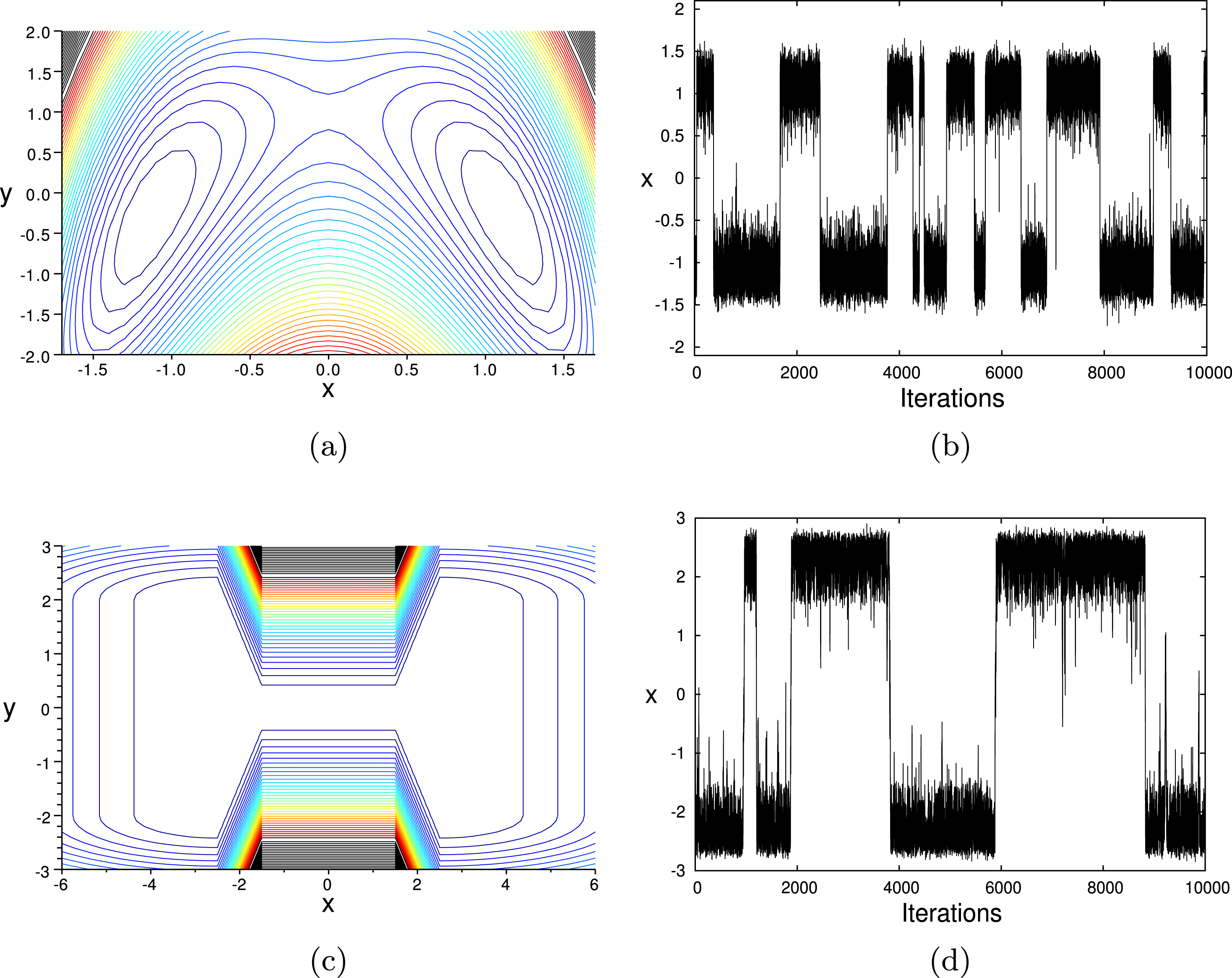
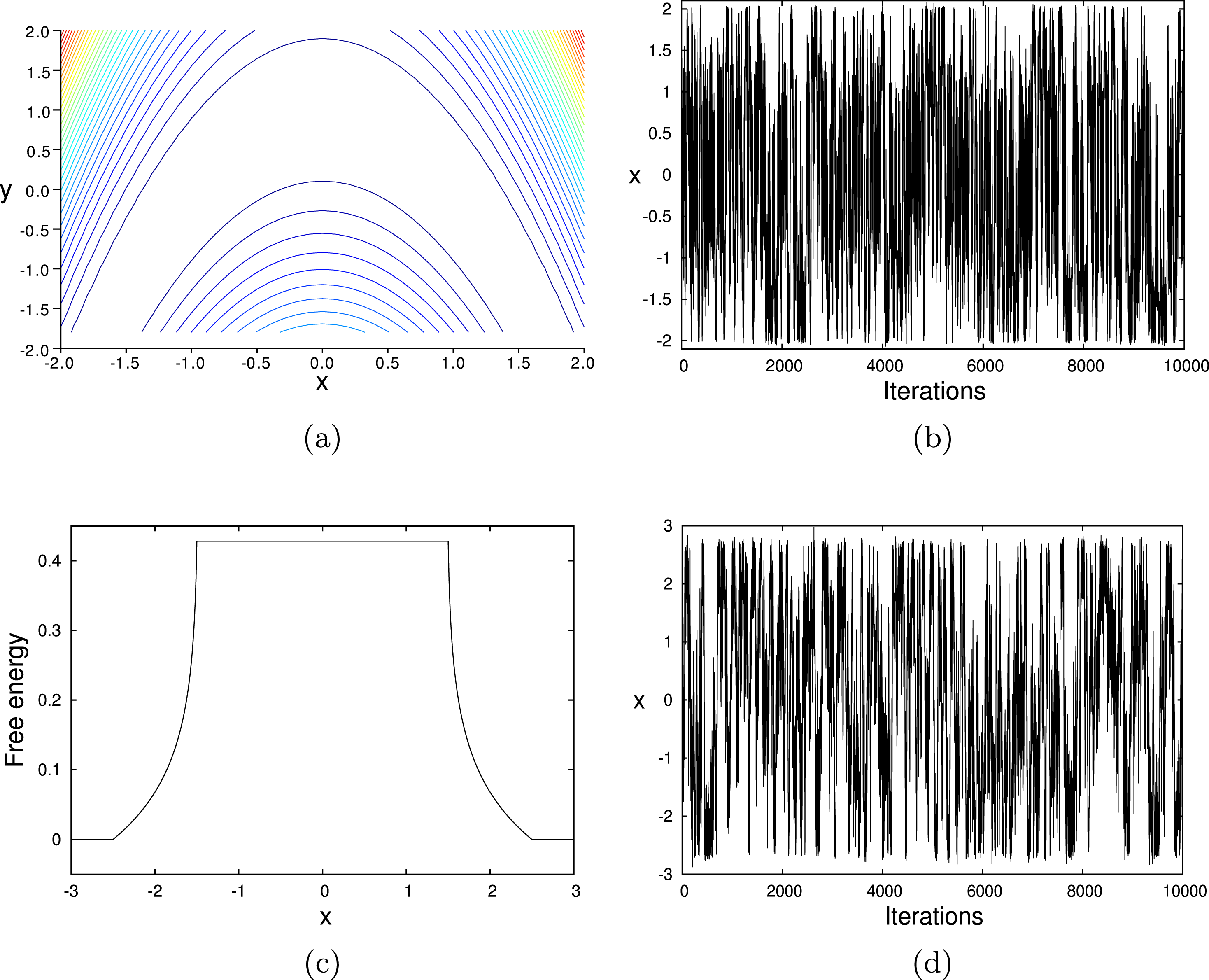
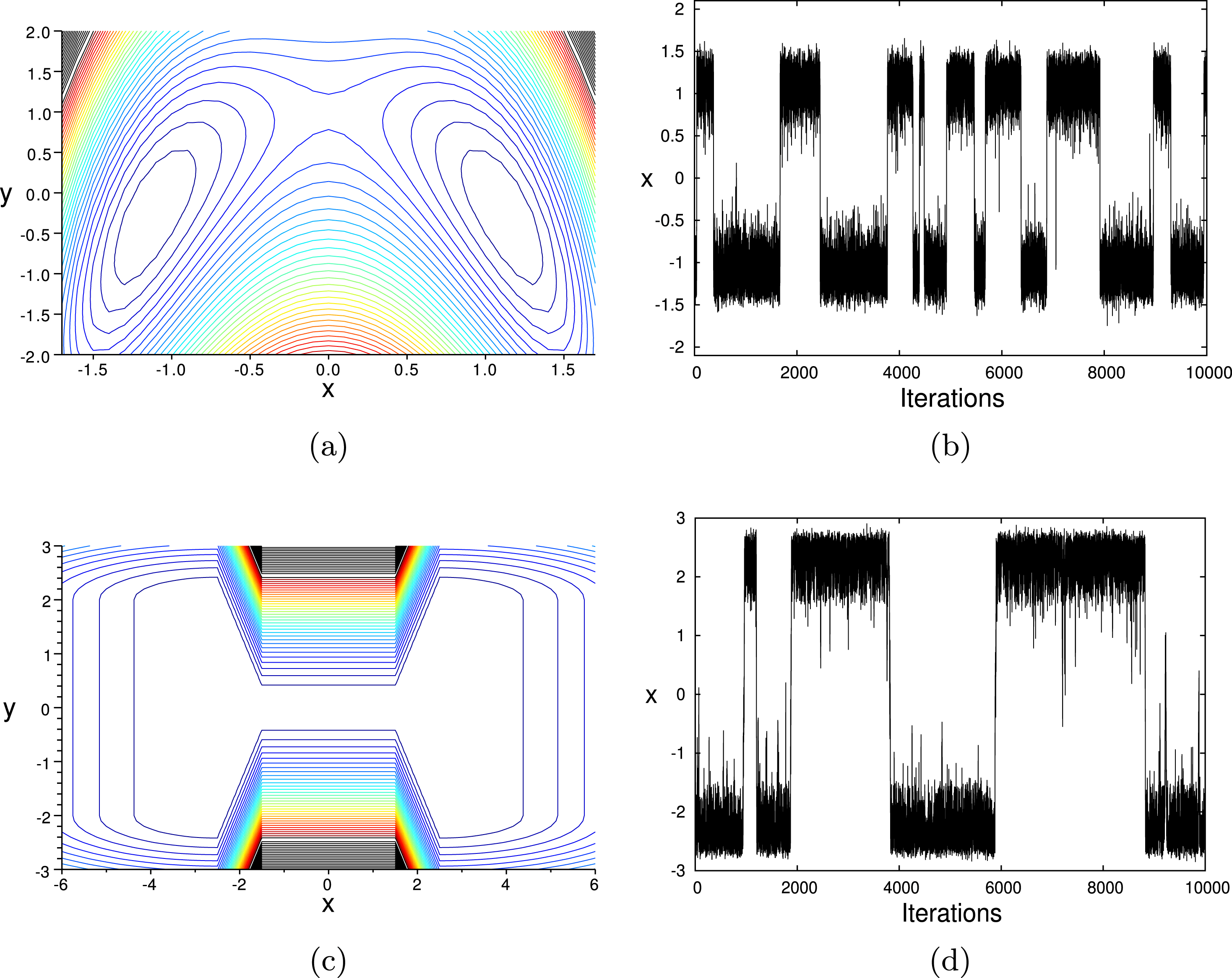
(a, c) Level sets of the two-dimensional potentials.
(b, d) Time evolution of the  $x$-coordinate of the stochastic process solution to
overdamped Langevin dynamics (1.8) in these potentials.
(a, b) Energetic barrier (
 ${\it\beta}=4$), (c, d) entropic barrier (
 ${\it\beta}=10$).
In terms of time scales, this discrepancy between the microscopic and the macroscopic scales is related to the fact that the stochastic processes that govern the evolutions of the positions of the particles are metastable: the system remains trapped for a long time in some region of the configurational space (called a metastable region) before hopping to another metastable region. Metastability implies that the convergence of averages over trajectories is slow, and that transitions between metastable regions are rare. As a simple illustration of metastability, let us present a two-dimensional example using overdamped Langevin dynamics (1.8), which we recall for convenience:
 $$\begin{eqnarray}\text{d}q_{t}=-{\rm\nabla}V(q_{t})\,\text{d}t+\sqrt{2{\it\beta}^{-1}}\,\text{d}W_{t}.\end{eqnarray}$$
In Figure 1.1 the
two origins of metastability are illustrated. First, as shown in
Figure 1.1(a, b),
the stochastic process  $(q_{t})_{t\geqslant 0}$ can be metastable because of energetic barriers: to migrate from
one metastable region to another, the process has to cross level sets of the
energy function
 $V$ and to overcome a first-order saddle point. Second,
metastability can be observed because of some steric constraints in the system. In
the example in Figure 1.1(c, d), the potential function is zero inside the
hourglass-shaped region and strongly repulsive outside this region. The stochastic
process
 $(q_{t})_{t\geqslant 0}$ is then a simple random walk in the region of zero potential. In
this case, metastability is observed because it takes a long time to find the
narrow corridor between the two metastable regions. Such potentials exhibit
so-called entropic barriers, since the accessible space for the system to leave a
metastable state is very small. These two types of metastable behaviour are
different in nature, and as will be explained below, this distinction is important
when discussing sampling techniques, since some of them are limited to energetic
barriers (see in particular Section 6). The difference between these two types of barrier is best seen by
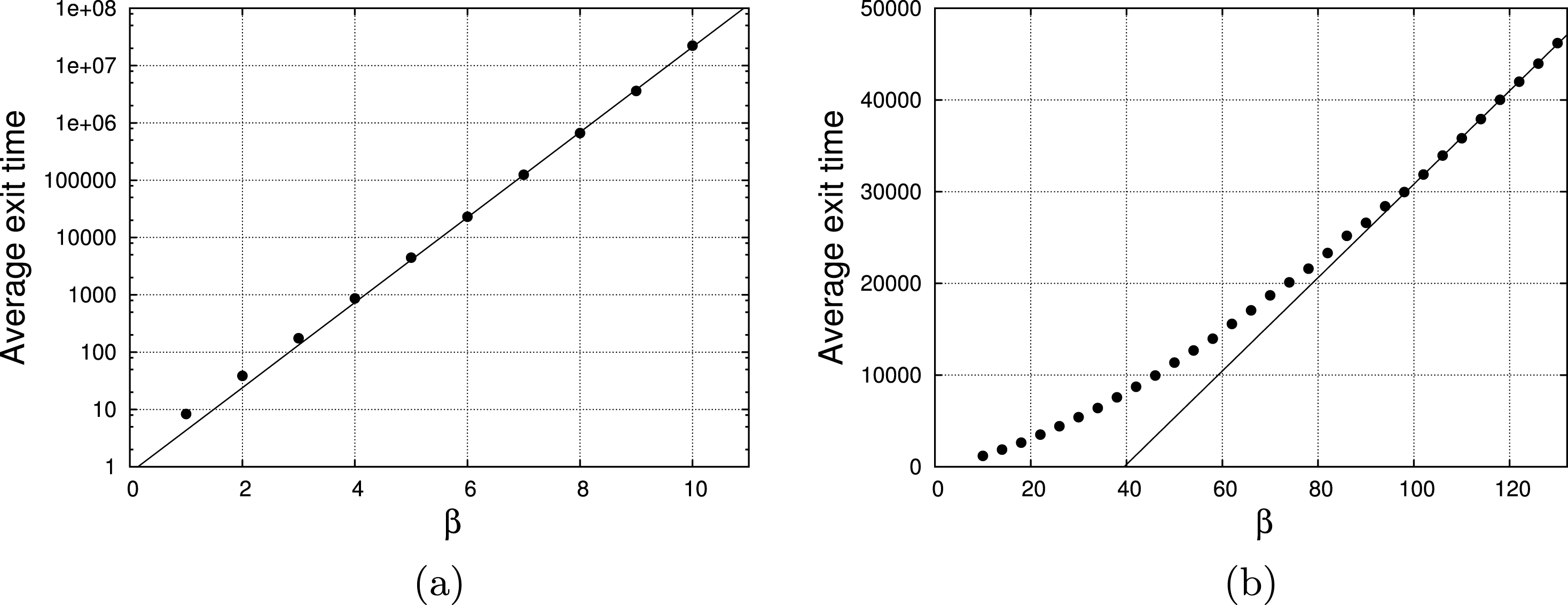
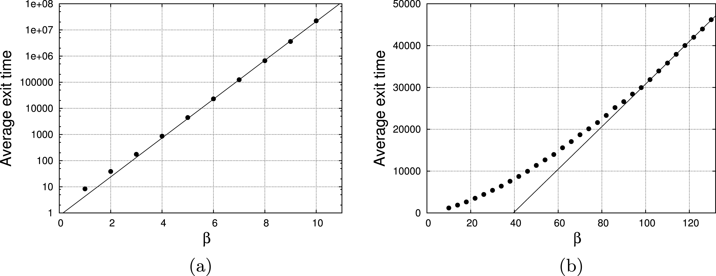
modifying the temperature. When the temperature decreases, the typical time scale
to leave a metastable region grows exponentially fast with respect to
 ${\it\beta}$ for energetic barriers, in accordance with results from large
deviation theory (Freidlin and Wentzell Reference Freidlin and Wentzell1984, Dembo and Zeitouni Reference Dembo and Zeitouni1998). For
an entropic barrier, such as that of Figure 1.1(c, d), a change in temperature is
(asymptotically) equivalent to a linear rescaling in time. These different
behaviours are illustrated in Figure 1.2. In terms of numerical approximations, metastability implies that
trajectory averages converge very slowly to their ergodic limits (the convergence
 $t\rightarrow \infty$ in (1.10) is
difficult to reach numerically), because one has to wait for the process to visit
all the metastable states sufficiently often. This explains the difficulties
encountered when evaluating thermodynamic quantities accurately. In addition,
metastability also implies that transitions between metastable states are rare
events, but these events are typically the phenomena of interest when considering
dynamical quantities. Metastability is thus at the heart of the numerical
challenges observed in molecular dynamics. Therefore, the mathematical analysis of
the efficiency of sampling algorithms requires us to quantify the metastability of
the sampling dynamics (Lelièvre Reference Lelièvre, Cangiani, Davidchack, Georgoulis, Gorban, Levesley and Tretyakov2013).
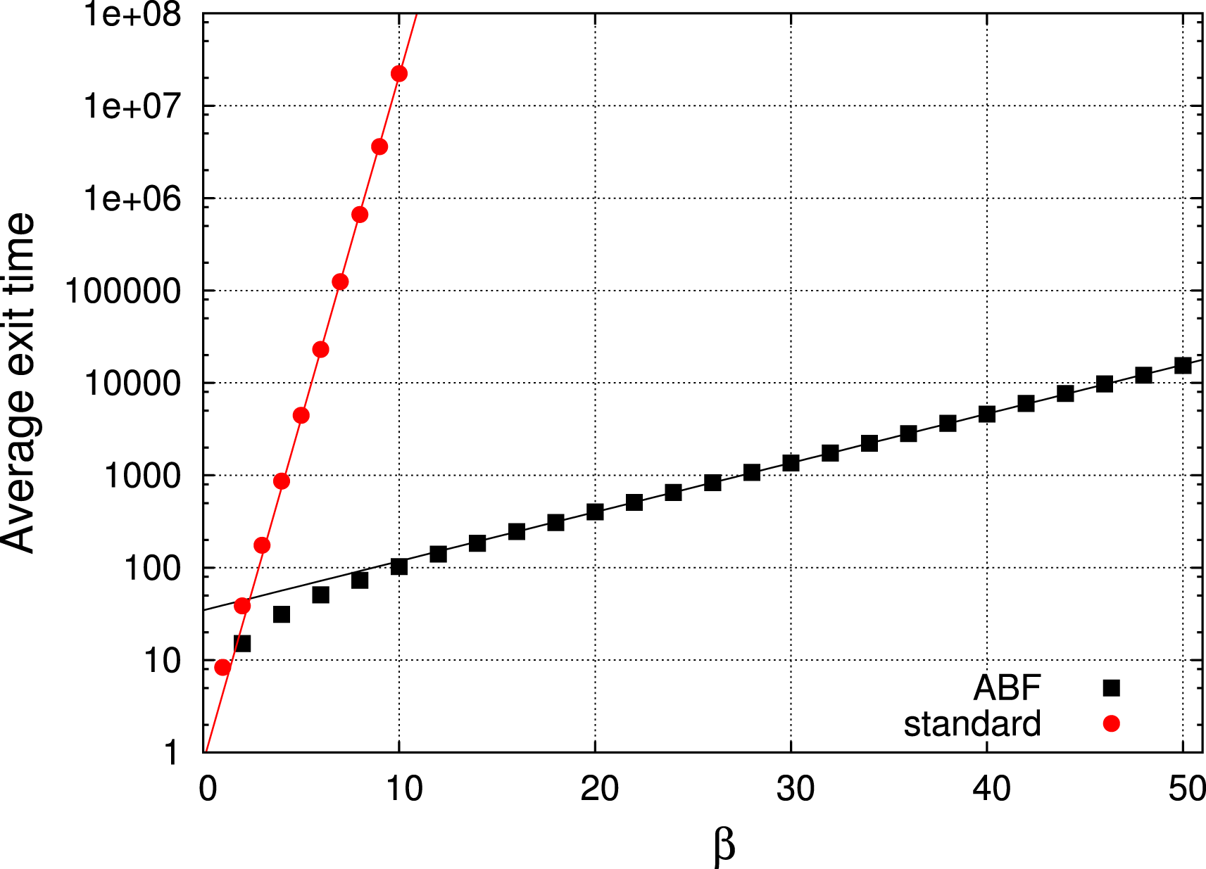
Average exit times  $\mathbb{E}({\it\tau})$ as a function of
 ${\it\beta}$, where
 ${\it\tau}=\inf \{t\geqslant 0\mid x_{t}\geqslant x_{\ast }\}$. (a) Energetic barrier (potential in
Figure 1.1(a)) with
 $x_{\ast }=1.3$ and initial conditions
 $x_{0}=(-1,0)$. The average exit times increase exponentially with
 ${\it\beta}$ (note the logarithmic scale on the ordinate axis).
(b) Entropic barrier (potential in Figure 1.1(c)) with
 $x_{\ast }=1.5$ and initial conditions
 $x_{0}=(-3,0)$. The average exit times increase linearly with
 ${\it\beta}$ for sufficiently large values of
 ${\it\beta}$.
As explained above, the metastability of the dynamics has some physical origin
(discrepancy of time scales between the microscopic and the macroscopic worlds).
From a purely numerical viewpoint, it is related to the multimodality of the
probability measure sampled by these dynamics. A probability measure is multimodal
if likely regions (modes) are separated by areas of small probabilities. Unless
deep knowledge of the system under study is available, two successive points
sampled by ergodic dynamics are very close to each other, because large uninformed
moves are very likely to fall in regions of small probability. This is why ergodic
dynamics with respect to a multimodal measure are in general metastable: it is
difficult to leave a mode of the target probability measure. This is closely
related to the difficulties associated with the global minimization of a function
in  $\mathbb{R}^{d}$ (in the limit
 ${\it\beta}\rightarrow \infty$, the measure
 ${\it\nu}$ is indeed a Dirac mass on the global minimum of
 $V$): a global optimization method should be able to find the global
minimum among all the local minima of the function (these local minima correspond
to different modes of the associated Boltzmann distribution (1.5)).
1.2.4 Other computational challenges
As explained above, the focus of this review is on sampling methods, and on PDE techniques to assess the quality of these methods. Before presenting how PDEs naturally appear in such a context, we would like to briefly discuss other computational challenges raised by molecular dynamics computations, though we will not discuss this further.
The integration of the deterministic Hamiltonian dynamics raises many interesting numerical questions. The original motivation was to understand the excellent energy conservation properties of the Störmer–Verlet method (Verlet Reference Verlet1967). With only one force evaluation at each time step, this numerical method indeed exhibits excellent energy preservation over very large time horizons. This stability property can be proved for the Störmer–Verlet method (and, more generally, symplectic integrators) using backward error analysis. This has been extended in various directions: for example, replacing symplecticity by symmetry, considering systems with constraints, or extending these results to Hamiltonian partial differential equations (see e.g. Faou Reference Faou2012 for Schrödinger equations). We refer to Marsden and West (Reference Marsden and West2001), Hairer, Lubich and Wanner (Reference Hairer, Lubich and Wanner2003), Leimkuhler and Reich (Reference Leimkuhler and Reich2004), Hairer, Lubich and Wanner (Reference Hairer, Lubich and Wanner2006) and Bond and Leimkuhler (Reference Bond and Leimkuhler2007) for an introduction to this branch of numerical analysis, called geometric numerical integration.
In order to reduce the dimensionality of the problem under consideration,
so-called coarse-graining techniques have been devised. Hopefully, while reducing
the number of degrees of freedom, one also expects to increase the stability
threshold on the time step, and thus to be able to reach larger time horizons.
Many ideas have been proposed along these lines. A typical idea, the
basis of dissipative particle dynamics (Hoogerbrugge and Koelman Reference Hoogerbrugge and Koelman1992, Español and Warren Reference Español and Warren1995), is first to replace a molecule, or a
group of molecules, by some effective particle, then to determine the interactions
between such particles as some effective interaction obtained by averaging over
the actual interactions of the fully detailed system it represents, and finally to
add some stochastic fluctuations accounting for the microscopic variability that
disappeared in the coarse-graining process. See also Kevrekidis and Samaey (Reference Kevrekidis and Samaey2009) and Rohrdanz, Zheng, Maggioni and
Clementi (Reference Rohrdanz, Zheng, Maggioni and Clementi2011), for example, for a few
selected works on coarse-graining in molecular simulation. Mathematical analysis
is needed in order to (i) derive good coarse-graining strategies with
certified error bounds, and (ii) propose appropriate schemes to use
these coarse-graining models. Coarse-grained models can be used as predictors, the
results of which are then refined in a corrector step by resorting to more
accurate models. Alternatively, it is possible to construct coupling strategies in
space in order to use coarse-grained models in some places while using finer
models in others – as in quasicontinuum methods, which couple atomistic
simulations with finite element discretizations (Luskin and Ortner Reference Luskin and Ortner2013). In some sense, the free energy
introduced in Section 4 or the
accelerated dynamics presented in Section 6.4 are also examples of coarse-graining strategies. In all
instances of coarse-graining, the main difficulty consists in selecting the
relevant degrees of freedom over which the coarse-graining procedure is performed
(for instance, anticipating our later discussion, the reaction coordinate  ${\it\xi}$ for free energy computation, or the set
 $S$ to exit from for metastable dynamics). Thus statistical methods
(such as clustering, manifold learning or hidden Markov chain approaches) should
play an increasingly important role in future, for example to extract the
metastable states from a long trajectory; see
e.g. Fischer et al. (Reference Fischer, Waldhausen, Horenko, Meerbach and Schütte2007).
To conclude this section, let us mention that the modelling issues raised by the quality of the empirical force fields become ever more crucial as longer time scales are reached. Notwithstanding the numerous examples where molecular dynamics computations have provided insights into molecular systems in biology or material sciences, many numerical experiments also show that better force fields need to be developed in order to reach the desirable level of accuracy in many applications. This includes improvement of the modelling of polarizability (see for instance Lipparini et al. Reference Lipparini, Lagardère, Raynaud, Stamm, Cancès, Mennucci, Schnieders, Ren, Maday and Piquemal2015), the construction of dedicated force fields for water molecules (see Wallqvist and Mountain Reference Wallqvist and Mountain1999 and Jorgensen and Tirado-Rives Reference Jorgensen and Tirado-Rives2005 for early review articles), and the development of reactive potentials able to describe chemical reactions (with variants and improvements of the REBO and ReaxFF potentials mentioned in Section 1.1). Appropriate functional forms of the potential functions as well as parameters should be dictated by electronic structure calculations, and validated using experiments. In this context, mathematics should help to (i) solve the electronic structure calculation efficiently, and (ii) develop coupling approaches between quantum calculations and molecular dynamics computations. Advanced optimization procedures should be useful for constructing suitable force fields from many data (quantum computations, experiments). In particular, machine learning techniques play an increasingly crucial role in the field (Rupp Reference Rupp2015).
1.3 Improving numerical methods in molecular dynamics: how PDEs can help
In order to show how PDE techniques are useful for understanding and improving numerical techniques in molecular dynamics, we first recall the link between SDEs and PDEs. We then present the structure of the remainder of the article.
1.3.1 Link between SDEs and PDEs
Consider the general time-homogeneous stochastic differential equation on  $\mathbb{R}^{d}$:
 $$\begin{eqnarray}\text{d}x_{t}=b(x_{t})\,\text{d}t+{\it\sigma}(x_{t})\,\text{d}W_{t},\end{eqnarray}$$
for a given initial condition  $x_{0}\in \mathbb{R}^{d}$ and standard Brownian motion
 $W_{t}\in \mathbb{R}^{m}$, and where
 $b:\mathbb{R}^{d}\rightarrow \mathbb{R}^{d}$ and
 ${\it\sigma}:\mathbb{R}^{d}\rightarrow \mathbb{R}^{d\times m}$ are assumed to be such that there exists a unique (strong)
solution to (1.11). For example,
the classical setting is to assume that
 $b$ and
 ${\it\sigma}$ are locally Lipschitz, which yields local-in-time existence up
to a (stochastic) explosion time, and then to prove that the existence is actually
global in time with appropriate Lyapunov functions; see for example Khasminskii
(Reference Khasminskii2012), Mao (Reference Mao2008) and Rey-Bellet (Reference Rey-Bellet, Attal, Joye and Pillet2006).
The stochastic differential equation (1.11) is naturally associated with a differential operator:
 $$\begin{eqnarray}{\mathcal{L}}=b\cdot {\rm\nabla}+\frac{1}{2}{\it\sigma}{\it\sigma}^{T}:{\rm\nabla}^{2},\end{eqnarray}$$
which is the infinitesimal generator of the Markov process  $(x_{t})_{t\geqslant 0}$ solution to (1.11). Here, the symbol
 $:$ denotes the Frobenius inner product. More explicitly, for a
given
 $C^{\infty }$ test function
 ${\it\varphi}:\mathbb{R}^{d}\rightarrow \mathbb{R}$, the operator
 ${\mathcal{L}}$ acts via
 $$\begin{eqnarray}{\mathcal{L}}{\it\varphi}=\mathop{\sum }_{i=1}^{d}b_{i}\partial _{x_{i}}{\it\varphi}+\frac{1}{2}\mathop{\sum }_{i=1}^{d}\mathop{\sum }_{j=1}^{d}\mathop{\sum }_{k=1}^{m}{\it\sigma}_{i,k}{\it\sigma}_{j,k}\partial _{x_{i},x_{j}}{\it\varphi}.\end{eqnarray}$$
For example, the generator of overdamped Langevin dynamics (1.8) is
 $$\begin{eqnarray}{\mathcal{L}}=-{\rm\nabla}V\cdot {\rm\nabla}+{\it\beta}^{-1}{\rm\Delta}={\it\beta}^{-1}\exp ({\it\beta}V)\text{div}[(\exp (-{\it\beta}V){\rm\nabla}\cdot ],\end{eqnarray}$$
while, for Langevin dynamics (1.9), we have
 $$\begin{eqnarray}\displaystyle {\mathcal{L}}=M^{-1}p\cdot {\rm\nabla}_{q}-{\rm\nabla}V\cdot {\rm\nabla}_{p}+{\it\gamma}(-M^{-1}p\cdot {\rm\nabla}_{p}+{\it\beta}^{-1}{\rm\Delta}_{p}). & & \displaystyle\end{eqnarray}$$
Here and elsewhere, we will always consider generators to be
defined on appropriate dense subsets of the domain of the generator, such as  $C^{\infty }$ functions with compact support or whose derivatives
grow at most polynomially.
The link between (1.11) and (1.12) is made explicit in the following lemma.
Lemma 1.1. Let  ${\it\varphi}$ be a compactly supported
 $C^{\infty }$ function. Then
 $$\begin{eqnarray}\frac{\text{d}}{\text{d}t}[\mathbb{E}^{x}({\it\varphi}(x_{t}))]\Big|_{t=0}={\mathcal{L}}{\it\varphi}(x),\end{eqnarray}$$
where the superscript  $x$ indicates that the initial condition of (1.11) is
 $x_{0}=x$, for a fixed
 $x\in {\mathcal{X}}$, and the expectation is taken over the Brownian paths.
The proof is a direct consequence of the Itô formula,
 $$\begin{eqnarray}\text{d}{\it\varphi}(x_{t})={\mathcal{L}}{\it\varphi}(x_{t})\,\text{d}t+({\rm\nabla}{\it\varphi}(x_{t}))^{T}{\it\sigma}(x_{t})\,\text{d}W_{t},\end{eqnarray}$$
and the fact that  ${\it\varphi}$ is
 $C^{\infty }$ and compactly supported, so that
 $$\begin{eqnarray}\mathbb{E}^{x}\biggl(\int _{0}^{t}({\rm\nabla}{\it\varphi}(x_{s}))^{T}{\it\sigma}(x_{s})\,\text{d}W_{s}\biggr)=0\end{eqnarray}$$
because the argument of the expectation is a square-integrable martingale (Revuz and Yor Reference Revuz and Yor1999). Therefore
 $$\begin{eqnarray}\mathbb{E}^{x}[{\it\varphi}(x_{t})]-{\it\varphi}(x)=\int _{0}^{t}\mathbb{E}^{x}[({\mathcal{L}}{\it\varphi})(x_{s})]\,\text{d}s,\end{eqnarray}$$
and the following limit is well defined:
 $$\begin{eqnarray}\frac{\text{d}}{\text{d}t}(\mathbb{E}^{x}[{\it\varphi}(x_{t})])\Big|_{t=0}=\lim _{t\rightarrow 0}\frac{\mathbb{E}^{x}[{\it\varphi}(x_{t})]-{\it\varphi}(x)}{t}={\mathcal{L}}{\it\varphi}(x).\end{eqnarray}$$
The infinitesimal generator  ${\mathcal{L}}$ associated with the stochastic dynamics plays a crucial role in
the following since it is the natural differential operator that appears in three
partial differential equations related to the stochastic dynamics: (i) the
Fokker–Planck dynamics that governs the evolution of the law of
 $x_{t}$ (see Section 2.1), (ii) the Poisson equation for the asymptotic variance of estimators
based on time averages (see Section 3.1), and (iii) the Feynman–Kac formula (see
Section 6.1).
Let us conclude this section by giving a very important characterization of the
invariance of a probability measure by a stochastic evolution in terms of the
generator:  ${\it\pi}$ is an invariant probability measure for (1.11) if and only if for any
 $C^{\infty }$ and compactly supported test function
 ${\it\varphi}$,
 $$\begin{eqnarray}\int _{{\mathcal{X}}}{\mathcal{L}}{\it\varphi}\,\text{d}{\it\pi}=0.\end{eqnarray}$$
This characterization directly follows from (1.15) by integrating both sides with
respect to  ${\it\pi}$, and using that
 $\mathbb{E}({\it\varphi}(x_{t}))=\mathbb{E}({\it\varphi}(x_{0}))$ when
 $x_{0}\sim {\it\pi}$ since, by definition of the invariance of the measure
 ${\it\pi}$, we have
 $x_{t}\sim {\it\pi}$. (Here and in the following, the notation
 $x\sim {\it\pi}$ means that the random variable
 $x$ is distributed according to the probability measure
 ${\it\pi}$.)
1.3.2 Assessing the efficiency and the accuracy of sampling algorithms
For the estimation of thermodynamic quantities, PDE techniques can be used in the following contexts.
∙ Determining (upper bounds to) the rate of convergence to equilibrium of stochastic dynamics. These rates of convergence can indeed be used to quantify the sampling efficiency of the underlying dynamics. The techniques used are typically functional inequalities allowing us to prove the existence of a spectral gap for the generator
${\mathcal{L}}$ (or equivalently the exponential convergence
to 0 of the associated semigroup $\text{e}^{t{\mathcal{L}}}$). Section 2 is devoted to these aspects for simple equilibrium dynamics.
Extensions to more complicated dynamics are possible: in
Section 4.3 we study
the long-time behaviour of the solution to a non-linear PDE by an
appropriate modification of one of the approaches used in the linear case
(entropy techniques).∙ Quantifying the errors in the computation of ensemble averages via ergodic averages over a single long trajectory (see Section 3). These errors are of two types: systematic errors arising from the bias on the invariant measure due to the time discretization of the continuous dynamics, and statistical errors governed by a central limit theorem. For systematic errors due to time discretization, the first PDE tool used for Langevin dynamics is a Trotter or Strang splitting of the semigroup to suggest new numerical schemes, or to analyse their accuracy. Second, a PDE is also involved when considering the solution of a Poisson equation of the form
${\mathcal{L}}u=f$ to characterize the leading error term on the invariant
measure. Poisson equations are also used to obtain the expression of the
asymptotic variance dictating the magnitude of the statistical error.


For the estimation of dynamical quantities, PDEs are useful in the following contexts.
∙ Defining transport coefficients, expressed either as integrated correlation functions or given by the linear response of non-equilibrium dynamics in the limit of small non-equilibrium forcings (see Section 5). The PDE technique used is perturbation theory of linear operators.
∙ Understanding the properties of algorithms for the sampling of paths (see Section 6.3). The results rely on the properties of solutions to the Hamilton–Jacobi–Bellman equation for variance reduction techniques based on importance sampling, while the analysis of the exit problem for accelerated dynamics starting in a metastable state relies on quasi-stationary distributions, which are eigenfunctions of Fokker–Planck equations with Dirichlet boundary conditions.
One topic that is also relevant to the analysis of metastable processes, and that we will discuss only briefly in this review (see Section 6.2), is the determination and computation of the rate functional in large deviation results (Freidlin and Wentzell Reference Freidlin and Wentzell1984, Olivieri and Vares Reference Olivieri and Vares2005). Let us only mention that the rate functional is determined for Markov processes by the Donsker–Varadhan formula (obtained in a series of works starting with Donsker and Varadhan Reference Donsker and Varadhan1975), which involves the generator of the dynamics. In addition, the variance of time averages computed along a single realization of the dynamics can be computed from the second derivative of this rate functional (den Hollander Reference den Hollander2000). This opens the way for variance reduction techniques based on large deviation results, relying on PDE techniques, as recently presented by Rey-Bellet and Spiliopoulos (Reference Rey-Bellet and Spiliopoulos2015).
1.3.3 Outline of this review
Section 2 gives the theoretical foundations needed in the next four sections. Sections 3 and 4 focus on the computation of thermodynamic quantities such as (1.3) and (1.4), while the estimation of dynamical quantities such as (1.7) is the subject of Sections 5 and 6. More precisely, we start in Section 2 by reviewing results on the long-time convergence of the laws of the stochastic processes under consideration. We then discuss in Section 3 the various errors arising in the computation of average properties along a single, long realization of some ergodic dynamics. Section 4 is devoted to the computation of free energy differences, for which dedicated techniques have to be used. The first dynamical quantities considered are transport coefficients in Section 5, numerically obtained either from dynamical information on equilibrium trajectories or from the linear response of steady-state non-equilibrium systems. Finally, in Section 6, we turn to the sampling of trajectories between metastable states.
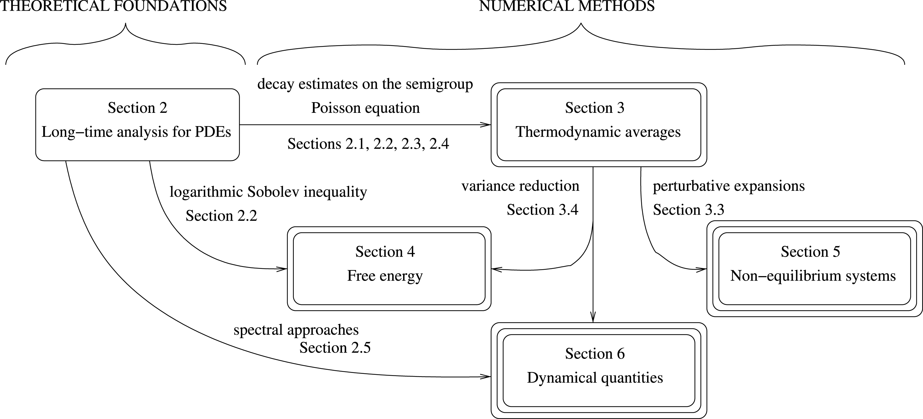
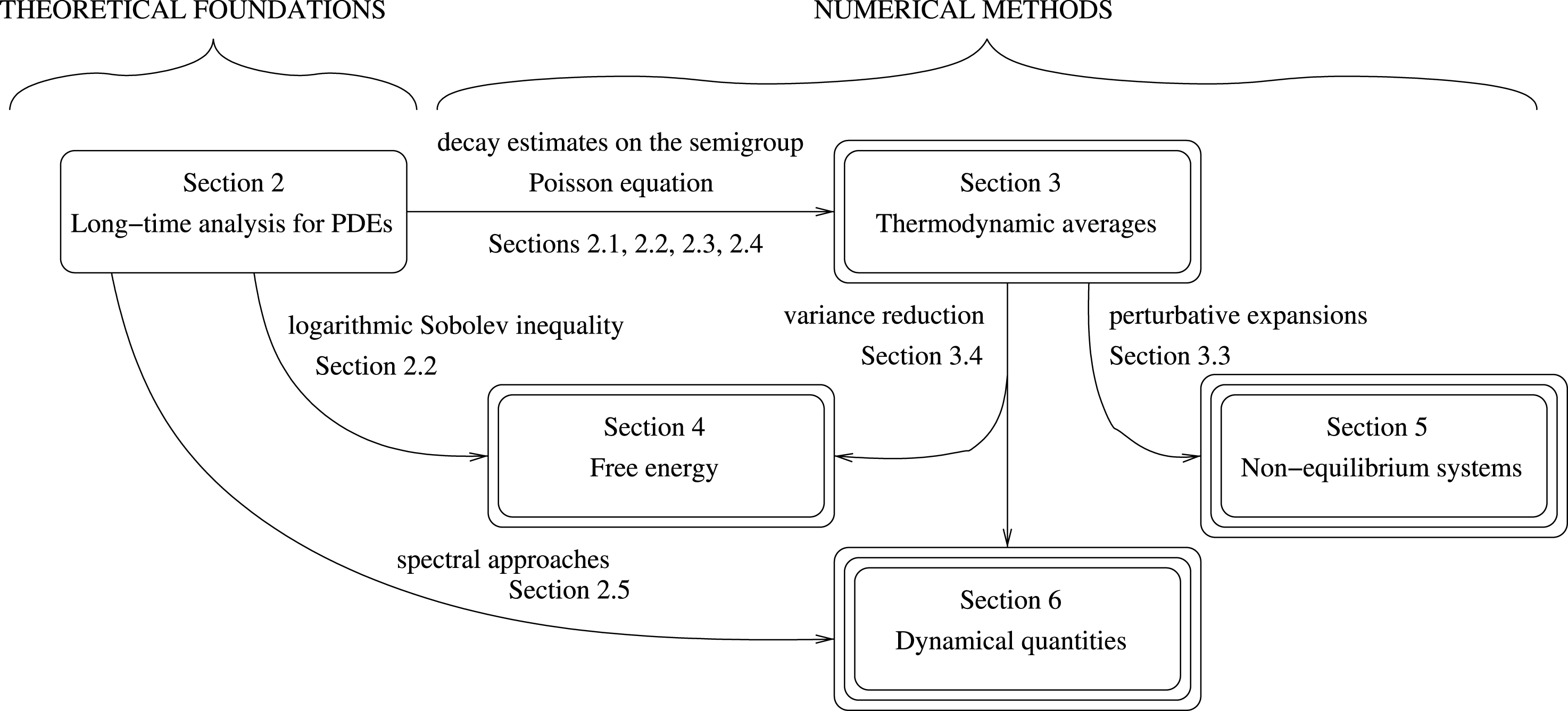
In Figure 1.3 we provide an overview of the interdependence of the sections, with an emphasis on the theoretical tools from Section 2 needed in the next four sections. The reader who is mostly interested in numerical methods can directly attack any of the four Sections 3, 4, 5 or 6, which are essentially independent, coming back to Section 2 when some theoretical background is needed.
Before getting to the heart of the matter, let us emphasize again that the focus of this review is on sampling methods used in molecular dynamics and which can be analysed using partial differential equations. Other sampling methods will therefore be mentioned only briefly, even though they may be equally important in practice. Moreover, for the sake of brevity, we sometimes present only the main arguments or ideas without the full mathematical details. In both cases, we give extensive references for further reading.
Interdependence of the sections. Double (respectively triple) boxes are
for sections devoted to the computation of thermodynamic quantities
(respectively dynamical quantities). In particular,
Section 3 mainly uses
decay estimates from Section 2 on the semigroup of the form  $\Vert \text{e}^{t{\mathcal{L}}}\Vert _{{\mathcal{B}}(E)}\leqslant C\,\text{e}^{-{\it\alpha}t}$ for some positive constants
 $C$ and
 ${\it\alpha}$, which in turn implies the well-posedness of the
Poisson equation
 ${\mathcal{L}}u=f$ in a certain Banach space
 $E$ (see Proposition 2.1 and Corollaries 2.4, 2.16, 2.21 and 2.27).
2 Long-time analysis for partial differential equations: some standard approaches
As explained above, one approach to studying the efficiency of a sampling method is to
study the rate of convergence to equilibrium of the law at time  $t$ of the process. The analysis techniques that have been developed to
study the long-time behaviour of solutions to partial differential equations are very
useful in this context. The law at time
 $t$ of a stochastic process
 $(x_{t})_{t\geqslant 0}$, following the general stochastic differential equation (1.11), indeed satisfies a partial
differential equation called the Fokker–Planck equation (see
Section 2.1). In this section we
review standard methods to prove the convergence of the law at time
 $t$ of stochastic processes to some invariant probability measure (in our
context, typically the canonical measure).
These convergence results also provide bounds on the inverse of the generator, which turn out to be useful in various contexts, for example to define asymptotic variances of ergodic averages (Section 3.1), to make precise biases on invariant measures of discretizations of continuous dynamics (Section 3.3), or to state linear response results for the invariant measure of perturbed dynamics (Section 5.2). Some of the convergence results can also be transferred to discrete-time dynamics, which allows us to ensure the existence and uniqueness of invariant probability measures for discretizations of SDEs, or to compute the variance of the corresponding ergodic averages.
Some techniques to analyse the long-time behaviour of the stochastic process are limited
to specific structural assumptions on the dynamics: Poincaré inequalities and
logarithmic Sobolev inequalities are useful for randomly perturbed gradient dynamics
such as overdamped Langevin dynamics (see Section 2.2), while hypocoercivity estimates are well suited to Langevin
dynamics (see Section 2.3). On the
other hand, some processes, such as those encountered by non-reversible perturbations of
Langevin and overdamped Langevin dynamics, may not have the appropriate structural
properties for the previously mentioned techniques. In this case, Lyapunov-type
approaches turn out to be versatile methods (see Section 2.4). Finally, in Section 2.5, we describe how results on the spectrum of the infinitesimal
generator of a stochastic process in the asymptotic regime  ${\it\beta}\rightarrow \infty$ can be useful for studying a metastable process.
2.1 The Kolmogorov forward equation
Let us consider a stochastic process  $(x_{t})_{t\geqslant 0}$ in
 $\mathbb{R}^{d}$, following the dynamics (1.11). Let us assume for simplicity that the law of
 $x_{t}$ at time
 $t$ has a density
 ${\it\psi}$ with respect to Lebesgue measure:Footnote 1
 $x_{t}$ is distributed according to
 ${\it\psi}(t,x)\text{d}x$. We also let
 ${\it\psi}(0,x)={\it\psi}_{0}(x)$ denote the density of the initial distribution. Then
 ${\it\psi}$ satisfies the Kolmogorov forward equation, also known as the
Fokker–Planck equation:
 $$\begin{eqnarray}\partial _{t}{\it\psi}={\mathcal{L}}^{\dagger }{\it\psi},\quad {\it\psi}(0)={\it\psi}_{0},\end{eqnarray}$$
where  ${\mathcal{L}}^{\dagger }$ denotes the
 $L^{2}$ adjoint of the operator
 ${\mathcal{L}}$:
 $$\begin{eqnarray}{\mathcal{L}}^{\dagger }=-\text{div}(b\,\cdot )+\frac{1}{2}{\rm\nabla}^{2}:({\it\sigma}{\it\sigma}^{T}\cdot ).\end{eqnarray}$$
Explicitly, for a given  $C^{\infty }$ test function
 ${\it\varphi}:\mathbb{R}^{d}\rightarrow \mathbb{R}$,
 $$\begin{eqnarray}{\mathcal{L}}^{\dagger }{\it\psi}=-\mathop{\sum }_{i=1}^{d}\partial _{x_{i}}(b_{i}{\it\psi})+\frac{1}{2}\mathop{\sum }_{i,j=1}^{d}\mathop{\sum }_{k=1}^{m}\partial _{x_{i},x_{j}}({\it\sigma}_{i,k}{\it\sigma}_{j,k}{\it\psi}).\end{eqnarray}$$
In particular, for overdamped Langevin dynamics (1.8), the density  ${\it\psi}(t,q)$ satisfies (2.1) with
 $$\begin{eqnarray}\displaystyle {\mathcal{L}}^{\dagger }{\it\psi}=\text{div}({\rm\nabla}V{\it\psi})+\frac{1}{{\it\beta}}{\rm\Delta}{\it\psi}=\frac{1}{{\it\beta}}\text{div}[\text{e}^{-{\it\beta}V}{\rm\nabla}(\text{e}^{{\it\beta}V}{\it\psi})]. & & \displaystyle\end{eqnarray}$$
For Langevin dynamics (1.9), the density  ${\it\psi}(t,q,p)$ satisfies (2.1) with
 $$\begin{eqnarray}\displaystyle {\mathcal{L}}^{\dagger }{\it\psi}=-p^{T}M^{-1}{\rm\nabla}_{q}{\it\psi}+{\rm\nabla}V^{T}{\rm\nabla}_{p}{\it\psi}+{\it\gamma}\,\text{div}_{p}\biggl(M^{-1}p\,{\it\psi}+\frac{1}{{\it\beta}}{\rm\nabla}_{p}{\it\psi}\biggr). & & \displaystyle\end{eqnarray}$$
The Fokker–Planck equation (2.1) is a consequence of (1.16). Indeed, for  $h>0$,
 $$\begin{eqnarray}\frac{\mathbb{E}^{x}[{\it\varphi}(x_{t+h})]-\mathbb{E}^{x}[{\it\varphi}(x_{t})]}{h}=\frac{1}{h}\int _{t}^{t+h}\mathbb{E}^{x}[({\mathcal{L}}{\it\varphi})(x_{s})]\,\text{d}s,\end{eqnarray}$$
which, after integration with respect to  ${\it\psi}_{0}$, gives
 $$\begin{eqnarray}\displaystyle & & \displaystyle \frac{1}{h}\biggl(\int _{\mathbb{R}^{d}}{\it\varphi}(x){\it\psi}(t+h,x)\,\text{d}x-\int _{\mathbb{R}^{d}}{\it\varphi}(x){\it\psi}(t,x)\,\text{d}x\biggr)\nonumber\\ \displaystyle & & \displaystyle \quad =\frac{1}{h}\int _{t}^{t+h}\int _{\mathbb{R}^{d}}({\mathcal{L}}{\it\varphi})(x){\it\psi}(s,x)\,\text{d}x\,\text{d}s.\nonumber\end{eqnarray}$$
This leads, in the limit  $h\rightarrow 0$, to the following equation:
 $$\begin{eqnarray}\frac{\text{d}}{\text{d}t}\biggl(\int _{\mathbb{R}^{d}}{\it\varphi}(x){\it\psi}(t,x)\,\text{d}x\biggr)=\int _{\mathbb{R}^{d}}({\mathcal{L}}{\it\varphi})(x){\it\psi}(t,x)\,\text{d}x,\end{eqnarray}$$
which is satisfied for all test functions  ${\it\varphi}$ (say,
 $C^{\infty }$ and compactly supported). This is indeed a weak formulation of
(2.1). For rigorous results
concerning the existence and uniqueness of a solution to (2.1) and the link with stochastic
differential equations, we refer for example to Friedman (Reference Friedman1975).
Let us mention that the invariance of the canonical measure  ${\it\nu}$ (resp.
 ${\it\mu}$) for overdamped Langevin dynamics (resp. Langevin
dynamics) is easily checked. A simple computation indeed shows that the canonical
measuresFootnote 2 are stationary solutions to (2.1), that is,
 $$\begin{eqnarray}\text{div}({\rm\nabla}V{\it\nu})+{\it\beta}^{-1}{\rm\Delta}{\it\nu}=0,\end{eqnarray}$$
and
 $$\begin{eqnarray}-M^{-1}p\cdot {\rm\nabla}_{q}{\it\mu}+{\rm\nabla}V\cdot {\rm\nabla}_{p}{\it\mu}+{\it\gamma}\text{div}(M^{-1}p{\it\mu}+{\it\beta}^{-1}{\rm\nabla}_{p}{\it\mu})=0,\end{eqnarray}$$
respectively.
When a reference probability measure  ${\it\pi}$ is given (typically, the canonical measure for Langevin or
overdamped Langevin dynamics), it is sometimes useful to consider the adjoint of the
generator
 ${\mathcal{L}}$ in the weighted
 $L^{2}$-space
 $$\begin{eqnarray}L^{2}({\it\pi})=\biggl\{{\it\varphi}:{\mathcal{X}}\rightarrow \mathbb{R}\,\text{measurable}\,\bigg|\,\int _{{\mathcal{X}}}|{\it\varphi}|^{2}\,\text{d}{\it\pi}<\infty \biggr\}.\end{eqnarray}$$
We let  ${\mathcal{L}}^{\ast }$ denote the adjoint of
 ${\mathcal{L}}$ on
 $L^{2}({\it\pi})$. For any
 $C^{\infty }$ and compactly supported functions
 ${\it\varphi},{\it\phi}$,
 $$\begin{eqnarray}\int _{{\mathcal{X}}}({\mathcal{L}}{\it\varphi}){\it\phi}\,\text{d}{\it\pi}=\int _{{\mathcal{X}}}{\it\varphi}({\mathcal{L}}^{\ast }{\it\phi})\,\text{d}{\it\pi}.\end{eqnarray}$$
In this framework, the invariance of  ${\it\pi}$ for the dynamics is formulated as
 ${\mathcal{L}}^{\ast }\mathbf{1}=0$, where
 $\mathbf{1}$ is the constant function equal to 1. This result is
obtained by setting
 ${\it\phi}=\mathbf{1}$ and using (1.17). For the overdamped Langevin dynamics (1.8) with invariant measure
 ${\it\nu}$ and generator
 ${\mathcal{L}}$ defined by (1.13), one can check that
 ${\mathcal{L}}^{\ast }={\mathcal{L}}$. For the Langevin dynamics (1.9) with invariant measure
 ${\it\mu}$ and generator
 ${\mathcal{L}}$ defined by (1.14), one can check that
 $$\begin{eqnarray}{\mathcal{L}}^{\ast }=-M^{-1}p\cdot {\rm\nabla}_{q}+{\rm\nabla}V\cdot {\rm\nabla}_{p}+{\it\gamma}(-M^{-1}p\cdot {\rm\nabla}_{p}+{\it\beta}^{-1}{\rm\Delta}_{p}).\end{eqnarray}$$
In the following sections we analyse the convergence to the canonical measure of the
solution  ${\it\psi}$ to the Fokker–Planck equation (2.1), for both overdamped Langevin and
Langevin dynamics. Using a semigroup representation, the question can be rephrased as
studying the convergence of
 $\text{e}^{t{\mathcal{L}}^{\dagger }}{\it\psi}_{0}$ to the invariant measure
 ${\it\pi}$ (which is
 ${\it\nu}$ or
 ${\it\mu}$ depending on the context).
2.1.1 A dual viewpoint
It is in fact sometimes useful to adopt a dual viewpoint, and to study the
convergence of observables rather than probability densities. This amounts to
analysing the convergence of  $\text{e}^{t{\mathcal{L}}}{\it\varphi}$ to
 $\int _{{\mathcal{X}}}{\it\varphi}\,\text{d}{\it\pi}$. To make this remark precise, let us first note thatFootnote 3
 $\text{e}^{t{\mathcal{L}}}$ indeed encodes the time evolution of observables since
 $$\begin{eqnarray}(\text{e}^{t{\mathcal{L}}}{\it\varphi})(x)=\mathbb{E}^{x}({\it\varphi}(x_{t})).\end{eqnarray}$$
To prove (2.8) we
start from Itô’s formula: for a fixed time  $t>0$, for a
 $C^{\infty }$ function
 ${\it\varphi}$, and
 $s\in [0,t]$, we have
 $$\begin{eqnarray}\text{d}(\text{e}^{(t-s){\mathcal{L}}}{\it\varphi}(x_{s}))=(-\partial _{t}+{\mathcal{L}})(\text{e}^{(t-s){\mathcal{L}}}{\it\varphi})(x_{s})\,\text{d}s+{\rm\nabla}(\text{e}^{(t-s){\mathcal{L}}}{\it\varphi})\cdot {\it\sigma}(x_{s})\,\text{d}W_{s},\end{eqnarray}$$
so that
 $$\begin{eqnarray}\mathbb{E}^{x}({\it\varphi}(x_{t}))-\text{e}^{t{\mathcal{L}}}{\it\varphi}(x)=\mathbb{E}^{x}\biggl(\int _{0}^{t}{\rm\nabla}(\text{e}^{(t-s){\mathcal{L}}}{\it\varphi})\cdot {\it\sigma}(x_{s})\,\text{d}W_{s}\biggr)=0.\end{eqnarray}$$
For a general stochastic differential equation, the exponential decay to
equilibrium of  $\text{e}^{t{\mathcal{L}}}$, seen as a bounded operator on a reflexive Banach space
 $E\subset L^{2}$, is equivalent to the exponential decay to equilibrium of
 $\text{e}^{t{\mathcal{L}}^{\dagger }}$ seen as a bounded operator on
 $E^{\prime }$, the dual of
 $E$. This equivalence is a consequence of the following equality:
for
 $C^{\infty }$ compactly supported test functions
 ${\it\varphi}$ and
 ${\it\psi}_{0}$,
 $$\begin{eqnarray}\mathbb{E}({\it\varphi}(x_{t}))=\int _{{\mathcal{X}}}\,\text{e}^{t{\mathcal{L}}}{\it\varphi}(x_{0}){\it\psi}_{0}(x_{0})\,\text{d}x_{0}=\int _{{\mathcal{X}}}{\it\varphi}(x)\,\text{e}^{t{\mathcal{L}}^{\dagger }}{\it\psi}_{0}(x)\,\text{d}x,\end{eqnarray}$$
where  $(x_{t})_{t\geqslant 0}$ satisfies (1.11) and the law of
 $x_{0}$ is
 ${\it\psi}_{0}(x)\,\text{d}x$. In the particular case of overdamped Langevin and Langevin
dynamics, the long-time behaviours of
 $\text{e}^{t{\mathcal{L}}}$ and
 $\text{e}^{t{\mathcal{L}}^{\dagger }}$ are in fact closely related thanks to simple algebraic
identities: see respectively (2.15) and (2.36)
below.
Note also that, upon replacing the observable  ${\it\varphi}$ with
 ${\it\varphi}-\int _{{\mathcal{X}}}{\it\varphi}\,\text{d}{\it\pi}$, it suffices to understand the convergence to 0 of
 $\text{e}^{t{\mathcal{L}}}{\it\varphi}$ for functions
 ${\it\varphi}$ with average 0 with respect to
 ${\it\pi}$.
2.1.2 Exponential convergence of semigroups and definition of inverses
We introduce the operator norm on the vector space  ${\mathcal{B}}(E)$ of bounded linear operators on a Banach space
 $E$, defined by
 $$\begin{eqnarray}\Vert {\mathcal{A}}\Vert _{{\mathcal{B}}(E)}=\sup _{g\neq 0}\frac{\Vert {\mathcal{A}}g\Vert _{E}}{\Vert g\Vert _{E}}.\end{eqnarray}$$
Recall that  ${\mathcal{B}}(E)$ equipped with this norm is a Banach space. As discussed at the
beginning of this section, it is important in various contexts to obtain bounds on
the inverse of the generator
 ${\mathcal{L}}$ on
 $E$. The Banach space
 $E$ is typically a subspace of functions with average 0
with respect to the invariant measure, otherwise
 $\text{e}^{t{\mathcal{L}}}{\it\varphi}$ does not converge to 0 as
 $t\rightarrow +\infty$.
The invertibility of the generator, and bounds on this inverse in  ${\mathcal{B}}(E)$, can be deduced from decay estimates on the semigroup, as is
made precise in the following result.
Proposition 2.1. Assume that
 $$\begin{eqnarray}\Vert \text{e}^{t{\mathcal{L}}}\Vert _{{\mathcal{B}}(E)}\leqslant C\,\text{e}^{-{\it\lambda}t}.\end{eqnarray}$$
Then the operator  ${\mathcal{L}}$ is invertible on
 $E$, and
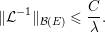 $$\begin{eqnarray}\Vert {\mathcal{L}}^{-1}\Vert _{{\mathcal{B}}(E)}\leqslant \frac{C}{{\it\lambda}}.\end{eqnarray}$$
Proof. Introducing
 $$\begin{eqnarray}U=-\int _{0}^{+\infty }\text{e}^{t{\mathcal{L}}}\,\text{d}t,\end{eqnarray}$$
a simple computation shows that, for  ${\it\varphi}\in D({\mathcal{L}})=\{{\it\phi}\in E\mid {\mathcal{L}}{\it\phi}\in E\}$,
 $$\begin{eqnarray}{\mathcal{L}}U{\it\varphi}=U{\mathcal{L}}{\it\varphi}=-\int _{0}^{+\infty }\frac{\text{d}}{\text{d}t}[\text{e}^{t{\mathcal{L}}}{\it\varphi}]={\it\varphi}.\end{eqnarray}$$
These equalities show that  ${\mathcal{L}}$ is invertible on
 $E$, with
 $U={\mathcal{L}}^{-1}$. From the definition of
 $U$, it follows that
 $$\begin{eqnarray}\Vert U\Vert _{{\mathcal{B}}(E)}\leqslant \int _{0}^{+\infty }\Vert \text{e}^{t{\mathcal{L}}}\Vert _{{\mathcal{B}}(E)}\,\text{d}t\leqslant C\int _{0}^{+\infty }\text{e}^{-{\it\lambda}t}\,\text{d}t=\frac{C}{{\it\lambda}},\end{eqnarray}$$
which proves the resolvent bound (2.10).
As a final remark, let us emphasize that the manipulations performed here for continuous-in-time dynamics can also be appropriately modified for discrete-in-time dynamics, such as encountered in the discretization of SDEs; see Corollary 2.26 below.
2.2 Poincaré and logarithmic Sobolev inequalities
We start by considering overdamped Langevin dynamics (1.8), the generator of which reads
 $$\begin{eqnarray}{\mathcal{L}}{\it\phi}=-{\rm\nabla}V\cdot {\rm\nabla}{\it\phi}+\frac{1}{{\it\beta}}{\rm\Delta}{\it\phi}=\frac{\text{e}^{{\it\beta}V}}{{\it\beta}}\text{div}(\text{e}^{-{\it\beta}V}{\rm\nabla}{\it\phi}).\end{eqnarray}$$
The associated Fokker–Planck equation is the parabolic PDE
 $$\begin{eqnarray}\partial _{t}{\it\psi}={\mathcal{L}}^{\dagger }{\it\psi},\quad {\it\psi}(0)={\it\psi}_{0},\end{eqnarray}$$
where  ${\mathcal{L}}^{\dagger }$ is introduced in (2.2), and the initial conditionFootnote 4
 ${\it\psi}_{0}\geqslant 0$ satisfies the normalization condition
 $$\begin{eqnarray}\int _{{\mathcal{D}}}{\it\psi}_{0}=1.\end{eqnarray}$$
We checked in (2.5) that the probability measure
 $$\begin{eqnarray}{\it\nu}(\text{d}q)=Z_{{\it\nu}}^{-1}\exp (-{\it\beta}V(q))\,\text{d}q\end{eqnarray}$$
is a stationary solution of the Fokker–Planck equation. It
is therefore relevant to ask whether  ${\it\psi}$ converges to
 ${\it\nu}$ and, if so, at what rate.
Before presenting several answers to this question, let us first give two
reformulations of the Fokker–Planck equation (2.12). A simple computation shows that
the function  $g={\it\psi}\,\text{e}^{{\it\beta}V/2}$ satisfies the Schrödinger-type equation
 $$\begin{eqnarray}\partial _{t}g=\frac{1}{{\it\beta}}{\rm\Delta}g+Wg,\quad W=\frac{1}{2}\biggl({\rm\Delta}V-\frac{{\it\beta}}{2}|{\rm\nabla}V|^{2}\biggr),\end{eqnarray}$$
together with the normalization condition
 $$\begin{eqnarray}\int _{{\mathcal{D}}}g(t)\,\text{e}^{-{\it\beta}V/2}=1,\quad \text{for all }t\geqslant 0.\end{eqnarray}$$
In addition, the function  $f={\it\psi}\,\text{e}^{{\it\beta}V}$ satisfies
 $$\begin{eqnarray}\partial _{t}f={\mathcal{L}}f,\quad \int _{{\mathcal{D}}}f\,\text{e}^{-{\it\beta}V}=1.\end{eqnarray}$$
In this last setting, the functional space to consider is the Hilbert space
 $$\begin{eqnarray}L^{2}({\it\nu})=\biggl\{{\it\varphi}\text{measurable}\,\bigg|\,\int _{{\mathcal{D}}}|{\it\varphi}|^{2}\,\text{d}{\it\nu}<+\infty \biggr\},\end{eqnarray}$$
equipped with the scalar productFootnote 5
 $$\begin{eqnarray}\langle {\it\varphi}_{1},{\it\varphi}_{2}\rangle _{L^{2}({\it\nu})}=\int _{{\mathcal{D}}}{\it\varphi}_{1}\,{\it\varphi}_{2}\,\text{d}{\it\nu}.\end{eqnarray}$$
A simple computation shows that  ${\mathcal{L}}$ is symmetric on
 $L^{2}({\it\nu})$. More precisely, for test functions
 ${\it\varphi}_{1},{\it\varphi}_{2}$ (
 $C^{\infty }$ and compactly supported),
 $$\begin{eqnarray}\langle {\mathcal{L}}{\it\varphi}_{1},{\it\varphi}_{2}\rangle _{L^{2}({\it\nu})}=\langle {\it\varphi}_{1},{\mathcal{L}}{\it\varphi}_{2}\rangle _{L^{2}({\it\nu})}=-\frac{1}{{\it\beta}}\int _{{\mathcal{D}}}{\rm\nabla}{\it\varphi}_{1}\cdot {\rm\nabla}{\it\varphi}_{2}\,\text{d}{\it\nu}.\end{eqnarray}$$
In fact, it can be proved that  ${\mathcal{L}}$ is self-adjoint on
 $L^{2}({\it\nu})$: see e.g. Bakry, Gentil and
Ledoux (Reference Bakry, Gentil and Ledoux2014).
2.2.1 Poincaré inequalities and convergence in $L^{2}({\it\nu})$

We start by considering the Fokker–Planck equation reformulated
as (2.15), for an
initial condition  $f_{0}={\it\psi}_{0}/{\it\nu}$ belonging to
 $L^{2}({\it\nu})$. Recall that
 $$\begin{eqnarray}f_{0}\geqslant 0,\quad \int _{{\mathcal{D}}}f_{0}\,\text{d}{\it\nu}=1.\end{eqnarray}$$
The simplest setting to consider is when a so-called
Poincaré inequality holds; see for instance Bakry
et al. (Reference Bakry, Gentil and Ledoux2014, Section 4) for a very nice introduction to these
inequalities. In this case,  $f(t)=\text{e}^{t{\mathcal{L}}}f_{0}$ converges exponentially fast in
 $L^{2}({\it\nu})$ to the constant function
 $\mathbf{1}$. This can be rephrased as the exponential convergence of
 $\text{e}^{t{\mathcal{L}}}(f_{0}-\mathbf{1})$ to 0 in
 $L^{2}({\it\nu})$.
In order to state the convergence result, we introduce the following definition.
Definition 2.2 (Poincaré inequality).
Consider the functional spaces
 $$\begin{eqnarray}L_{0}^{2}({\it\nu})=\biggl\{{\it\varphi}\in L^{2}({\it\nu})\,\bigg|\,\int _{{\mathcal{D}}}{\it\varphi}\,\text{d}{\it\nu}=0\biggr\},\end{eqnarray}$$
and
 $$\begin{eqnarray}H^{1}({\it\nu})=\biggl\{{\it\varphi}\in L^{2}({\it\nu})\,\bigg|\,{\rm\nabla}{\it\varphi}\in (L^{2}({\it\nu}))^{d}\biggr\}.\end{eqnarray}$$
The measure  ${\it\nu}$ is said to satisfy a Poincaré inequality with constant
 $R>0$ when
 $$\begin{eqnarray}\Vert {\it\varphi}\Vert _{L^{2}({\it\nu})}^{2}\leqslant \frac{1}{2R}\Vert {\rm\nabla}{\it\varphi}\Vert _{L^{2}({\it\nu})}^{2},\quad \text{for all }{\it\varphi}\in H^{1}({\it\nu})\cap L_{0}^{2}({\it\nu}).\end{eqnarray}$$
The constant  $R>0$ depends on the potential
 $V$, the inverse temperature
 ${\it\beta}$ and the domain
 ${\mathcal{D}}$. We discuss below various sufficient conditions for
 ${\it\nu}$ to satisfy a Poincaré inequality.
The inequality (2.17)
implies (and in fact is equivalent to) the exponential convergence to 0
of the semigroup  $\text{e}^{t{\mathcal{L}}}$ considered as an operator on
 $L_{0}^{2}({\it\nu})$.
Proposition 2.3. The measure  ${\it\nu}$ satisfies a Poincaré inequality with constant
 $R>0$ if and only if
 $$\begin{eqnarray}\Vert \text{e}^{t{\mathcal{L}}}\Vert _{{\mathcal{B}}(L_{0}^{2}({\it\nu}))}\leqslant \text{e}^{-2Rt/{\it\beta}}.\end{eqnarray}$$
Proof. Let us first assume that the measure  ${\it\nu}$ satisfies a Poincaré inequality with constant
 $R>0$. In view of (2.16),
 $$\begin{eqnarray}-\langle {\mathcal{L}}{\it\varphi},{\it\varphi}\rangle _{L^{2}({\it\nu})}=\frac{1}{{\it\beta}}\Vert {\rm\nabla}{\it\varphi}\Vert _{L^{2}({\it\nu})}^{2}\geqslant \frac{2R}{{\it\beta}}\Vert {\it\varphi}\Vert _{L^{2}({\it\nu})}^{2},\quad \text{for all }{\it\varphi}\in L_{0}^{2}({\it\nu})\cap H^{1}({\it\nu}).\end{eqnarray}$$
Since 0 is an eigenvalue of the operator  ${\mathcal{L}}$ (whose associated eigenvectors are constant functions),
this inequality shows that the spectral gap of the self-adjoint operator
 $-{\mathcal{L}}$ on
 $L^{2}({\it\nu})$ is larger than or equal to
 $2R/{\it\beta}$ (see (2.82) and the discussion following this equality). The inequality
(2.19) also gives the
exponential decrease of the semigroup on
 $L_{0}^{2}({\it\nu})$ since
 $$\begin{eqnarray}\frac{\text{d}}{\text{d}t}\biggl(\displaystyle \frac{1}{2}\Vert \text{e}^{t{\mathcal{L}}}{\it\varphi}\Vert _{L^{2}({\it\nu})}^{2}\biggr)=\langle \text{e}^{t{\mathcal{L}}}{\it\varphi},{\mathcal{L}}\,\text{e}^{t{\mathcal{L}}}{\it\varphi}\rangle _{L^{2}({\it\nu})}\leqslant -\frac{2R}{{\it\beta}}\Vert \text{e}^{t{\mathcal{L}}}{\it\varphi}\Vert _{L^{2}({\it\nu})}^{2}.\end{eqnarray}$$
By a Gronwall inequality, it follows that
 $$\begin{eqnarray}\Vert \text{e}^{t{\mathcal{L}}}{\it\varphi}\Vert _{L_{0}^{2}({\it\nu})}\leqslant \text{e}^{-2Rt/{\it\beta}}\Vert {\it\varphi}\Vert _{L_{0}^{2}({\it\nu})},\quad \text{for any }{\it\varphi}\in L_{0}^{2}({\it\nu}).\end{eqnarray}$$
Assume now that  $\Vert \text{e}^{t{\mathcal{L}}}\Vert _{{\mathcal{B}}(L_{0}^{2}({\it\nu}))}\leqslant \text{e}^{-2Rt/{\it\beta}}$. Then, for a given
 ${\it\varphi}\in L_{0}^{2}({\it\nu})$ and any
 $t>0$,
 $$\begin{eqnarray}\frac{\Vert \text{e}^{t{\mathcal{L}}}{\it\varphi}\Vert _{L_{0}^{2}({\it\nu})}^{2}-\Vert {\it\varphi}\Vert _{L_{0}^{2}({\it\nu})}^{2}}{t}\leqslant \Vert {\it\varphi}\Vert _{L_{0}^{2}({\it\nu})}^{2}\,\frac{\text{e}^{-4Rt/{\it\beta}}-1}{t}.\end{eqnarray}$$
We next pass to the limit  $t\rightarrow 0$, using the equalities in (2.19) and (2.20):
 $$\begin{eqnarray}-\frac{2}{{\it\beta}}\Vert {\rm\nabla}{\it\varphi}\Vert _{L^{2}({\it\nu})}^{2}\leqslant -\frac{4R}{{\it\beta}}\Vert {\it\varphi}\Vert _{L_{0}^{2}({\it\nu})}^{2}.\end{eqnarray}$$
Since  ${\it\varphi}\in L_{0}^{2}({\it\nu})$ is arbitrary, the Poincaré inequality (2.17) follows.
In view of Proposition 2.1, a useful corollary of the decay estimates on the semigroup is the following result.
Corollary 2.4. Assume that  ${\it\nu}$ satisfies a Poincaré inequality with constant
 $R$. Then the operator
 ${\mathcal{L}}$ is invertible on
 $L_{0}^{2}({\it\nu})$, and the following equality holds in
 ${\mathcal{B}}(L_{0}^{2}({\it\nu}))$:
 $$\begin{eqnarray}{\mathcal{L}}^{-1}=-\int _{0}^{+\infty }\,\text{e}^{t{\mathcal{L}}}\,\text{d}t.\end{eqnarray}$$
Moreover,
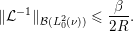 $$\begin{eqnarray}\Vert {\mathcal{L}}^{-1}\Vert _{{\mathcal{B}}(L_{0}^{2}({\it\nu}))}\leqslant \frac{{\it\beta}}{2R}.\end{eqnarray}$$
Let us now give some sufficient conditions to obtain Poincaré
inequalities. First, such inequalities are easily obtained for probability
measures equivalent to the Lebesgue measure, on connected domains, as a
consequence of the standard Poincaré–Wirtinger inequality.
This is the case when  ${\mathcal{D}}=(L\mathbb{T})^{d}$, for example. Indeed, consider a measure with density
 ${\it\rho}(q)$ with respect to Lebesgue measure, and such that there exist two
positive constants
 ${\it\rho}_{\min }$ and
 ${\it\rho}_{\max }$ with
 $0<{\it\rho}_{\min }\leqslant {\it\rho}(q)\leqslant {\it\rho}_{\max }$ for all
 $q\in {\mathcal{D}}$. First, note that
 $$\begin{eqnarray}\min _{c\in \mathbb{R}}\int _{{\mathcal{D}}}({\it\varphi}-c)^{2}\,\text{d}{\it\rho}=\int _{{\mathcal{D}}}({\it\varphi}-\mathbb{E}_{{\it\rho}}({\it\varphi}))^{2}\,\text{d}{\it\rho},\quad \text{for all }{\it\varphi}\in L^{2}({\it\rho}).\end{eqnarray}$$
Therefore,
 $$\begin{eqnarray}\displaystyle \min _{c\in \mathbb{R}}\int _{{\mathcal{D}}}({\it\varphi}-c)^{2}\,\text{d}{\it\rho} & {\leqslant} & \displaystyle {\it\rho}_{\max }\min _{c\in \mathbb{R}}\int _{{\mathcal{D}}}({\it\varphi}-c)^{2}\leqslant \frac{1}{2R_{\text{PW}}}{\it\rho}_{\max }\int _{{\mathcal{D}}}|{\rm\nabla}{\it\varphi}|^{2}\nonumber\\ \displaystyle & {\leqslant} & \displaystyle \frac{1}{2R_{\text{PW}}}\frac{{\it\rho}_{\max }}{{\it\rho}_{\min }}\int _{{\mathcal{D}}}|{\rm\nabla}{\it\varphi}|^{2}\,\text{d}{\it\rho},\nonumber\end{eqnarray}$$
where  $R_{\text{PW}}$ is the constant of the standard
Poincaré–Wirtinger inequality on the bounded, connected domain
 ${\mathcal{D}}$. This shows that the canonical measure
 ${\it\nu}$ defined in (2.13) satisfies a Poincaré inequality when the domain
 ${\mathcal{D}}$ is bounded, with the following upper bound for the
Poincaré constant
 $R_{{\it\nu}}$:
 $$\begin{eqnarray}R_{{\it\nu}}\leqslant R_{\text{PW}}\,\text{e}^{-{\it\beta}(V_{\max }-V_{\min })},\end{eqnarray}$$
where
 $$\begin{eqnarray}V_{\max }=\max _{q\in {\mathcal{D}}}V(q),\quad V_{\min }=\min _{q\in {\mathcal{D}}}V(q).\end{eqnarray}$$
In fact, this argument can be made more general to show that Poincaré inequalities satisfy some stability property under bounded perturbations of the measure, similar to the result obtained in Theorem 2.11 below for logarithmic Sobolev inequalities.
On unbounded domains, some conditions on the potential  $V$ are required to have a Poincaré inequality. For
example, such an inequality holds when
 $V$ is uniformly convex (i.e.,
 ${\rm\nabla}^{2}V\geqslant R\,\text{Id}_{d}$ with
 $R>0$), similar to the result stated in Theorem 2.10 below for logarithmic Sobolev
inequalities. Another result is based on the growth at infinity of the
potential: see Bakry, Barthe, Cattiaux and Guillin (Reference Bakry, Barthe, Cattiaux and Guillin2008, Corollary 1.6).
Theorem 2.5. Consider  $V\in C^{2}(\mathbb{R}^{d})$. If there exists
 $a\in (0,1)$,
 $c>0$ and
 $R\geqslant 0$ such that
 $$\begin{eqnarray}a{\it\beta}|{\rm\nabla}V(q)|^{2}-{\rm\Delta}V(q)\geqslant c,\quad \text{for all }q\in \mathbb{R}^{d}\text{ such that }|q|\geqslant R,\end{eqnarray}$$
then  ${\it\nu}$ satisfies a Poincaré inequality.
The above condition is satisfied, for instance, for potentials of the form
 $$\begin{eqnarray}V(q)=K|q|^{n}+\widetilde{V}(q),\end{eqnarray}$$
where  $n\geqslant 1$ and
 $\widetilde{V}$ is
 $C^{\infty }$ and such that
 $$\begin{eqnarray}\lim _{|q|\rightarrow +\infty }\frac{|\widetilde{V}(q)|}{|q|^{n}}=0\quad \text{and}\quad \lim _{|q|\rightarrow +\infty }\frac{|{\rm\nabla}\widetilde{V}|^{2}+|{\rm\Delta}\widetilde{V}|}{|q|^{2(n-1)}}=0.\end{eqnarray}$$
The first condition implies that  $\text{e}^{-{\it\beta}V}$ is integrable, while the second one ensures that (2.22) holds.
A useful result that we shall exploit below is that it is possible to deduce Poincaré inequalities by tensorization.
Proposition 2.6. If a probability measure is a product of  $d$ probability measures satisfying Poincaré
inequalities with constants
 $R_{i}$, then the product measure satisfies a Poincaré
inequality with constant
 $$\begin{eqnarray}\min (R_{1},\ldots ,R_{d}).\end{eqnarray}$$
Proof. To simplify the notation, we prove the result in the case  $d=2$, for a probability measure
 ${\it\rho}(\text{d}q_{1}\,\text{d}q_{2})={\it\rho}_{1}(\text{d}q_{1})\,{\it\rho}_{2}(\text{d}q_{2})$, defined on
 ${\mathcal{D}}={\mathcal{D}}_{1}\times {\mathcal{D}}_{2}$. Consider a
 $C^{\infty }$ function
 ${\it\varphi}$ with compact support, and average 0 with
respect to
 ${\it\rho}$. We first introduce the partial average
 $$\begin{eqnarray}\overline{{\it\varphi}}(q_{2})=\int _{{\mathcal{D}}_{1}}{\it\varphi}(q_{1}^{\prime },q_{2})\,{\it\rho}_{1}(\text{d}q_{1}^{\prime }).\end{eqnarray}$$
Since  ${\it\rho}_{1}$ satisfies a Poincaré inequality with constant
 $R_{1}$, and using the fact that the function
 $q_{1}\mapsto {\it\varphi}(q_{1},q_{2})-\overline{{\it\varphi}}(q_{2})$ has average 0 with respect to
 ${\it\rho}_{1}(\text{d}q_{1})$ for any value of
 $q_{2}$, we obtain
 $$\begin{eqnarray}\int _{{\mathcal{D}}_{1}}|{\it\varphi}(q_{1},q_{2})-\overline{{\it\varphi}}(q_{2})|^{2}{\it\rho}_{1}(\text{d}q_{1})\leqslant \frac{1}{2R_{1}}\int _{{\mathcal{D}}_{1}}|{\rm\nabla}_{q_{1}}{\it\varphi}(q_{1},q_{2})|^{2}{\it\rho}_{1}(\text{d}q_{1}).\end{eqnarray}$$
This inequality can be rewritten as
 $$\begin{eqnarray}\int _{{\mathcal{D}}_{1}}|{\it\varphi}(q_{1},q_{2})|^{2}{\it\rho}_{1}(\text{d}q_{1})\leqslant |\overline{{\it\varphi}}(q_{2})|^{2}+\frac{1}{2R_{1}}\int _{{\mathcal{D}}_{1}}|{\rm\nabla}_{q_{1}}{\it\varphi}(q_{1},q_{2})|^{2}{\it\rho}_{1}(\text{d}q_{1}).\end{eqnarray}$$
Now, since  $\overline{{\it\varphi}}$ has average 0 with respect to
 ${\it\rho}_{2}$ because
 ${\it\varphi}$ has average 0 with respect to
 ${\it\rho}$,
 $$\begin{eqnarray}\displaystyle \int _{{\mathcal{D}}_{2}}|\overline{{\it\varphi}}(q_{2})|^{2}{\it\rho}_{2}(\text{d}q_{2}) & {\leqslant} & \displaystyle \frac{1}{2R_{2}}\int _{{\mathcal{D}}_{2}}|{\rm\nabla}_{q_{2}}\overline{{\it\varphi}}(q_{2})|^{2}{\it\rho}_{2}(\text{d}q_{2})\nonumber\\ \displaystyle & {\leqslant} & \displaystyle \frac{1}{2R_{2}}\int _{{\mathcal{D}}}|{\rm\nabla}_{q_{2}}{\it\varphi}(q_{1},q_{2})|^{2}{\it\rho}_{1}(\text{d}q_{1})\,{\it\rho}_{2}(\text{d}q_{2}),\nonumber\end{eqnarray}$$
where we used a Cauchy–Schwarz inequality in the
last step. Integration of (2.23) with respect to  ${\it\rho}_{2}(\text{d}q_{2})$ finally leads to
 $$\begin{eqnarray}\displaystyle \int _{{\mathcal{D}}}|{\it\varphi}(q_{1},q_{2})|^{2}{\it\rho}(\text{d}q) & {\leqslant} & \displaystyle \frac{1}{2R_{1}}\int _{{\mathcal{D}}}|{\rm\nabla}_{q_{1}}{\it\varphi}(q_{1},q_{2})|^{2}{\it\rho}(\text{d}q)\nonumber\\ \displaystyle & & \displaystyle \quad +\frac{1}{2R_{2}}\int _{{\mathcal{D}}}|{\rm\nabla}_{q_{2}}{\it\varphi}(q_{1},q_{2})|^{2}{\it\rho}(\text{d}q)\nonumber\\ \displaystyle & & \displaystyle \leqslant \frac{1}{2\min (R_{1},R_{2})}\int _{{\mathcal{D}}}|{\rm\nabla}_{q}{\it\varphi}|^{2}\,\text{d}{\it\rho},\nonumber\end{eqnarray}$$
from which we deduce that  ${\it\rho}$ satisfies a Poincaré inequality with constant
 $R=\min (R_{1},R_{2})$.
Finally, anticipating later discussion, we will see in Proposition 2.12 that the logarithmic Sobolev inequality implies the Poincaré inequality.
2.2.2 Logarithmic Sobolev inequalities and convergence in $L^{1}({\it\nu})$

Here we give some background on logarithmic Sobolev inequalities, which can be used to show convergence to the equilibrium state. More material can be read in the review papers by Guionnet and Zegarlinski (Reference Guionnet and Zegarlinski2003), Ledoux (Reference Ledoux2001) and Arnold, Markowich, Toscani and Unterreiter (Reference Arnold, Markowich, Toscani and Unterreiter2001), and in Bakry et al. (Reference Bakry, Gentil and Ledoux2014, Section 5). The latter two works have a PDE approach which may be more appealing to readers accustomed to analytical frameworks. Other useful introductory references include Ané et al. (Reference Ané, Blachère, Chafaï, Fougères, Gentil, Malrieu, Roberto and Scheffer2000) and Villani (Reference Villani2003).
The relative entropy and the Fisher information between two measures are defined as follows.
Definition 2.7 (entropy and Fisher information).
For two probability measures  ${\it\pi}_{1}$ and
 ${\it\pi}_{2}$ defined on a space
 ${\mathcal{X}}$, and such that
 ${\it\pi}_{1}$ is absolutely continuous with respect to
 ${\it\pi}_{2}$ (denoted
 ${\it\pi}_{1}\ll {\it\pi}_{2}$ in the following), the entropy of
 ${\it\pi}_{1}$ with respect to
 ${\it\pi}_{2}$ is
 $$\begin{eqnarray}{\mathcal{H}}({\it\pi}_{1}\mid {\it\pi}_{2})=\int _{{\mathcal{X}}}\ln \biggl(\displaystyle \frac{\text{d}{\it\pi}_{1}}{\text{d}{\it\pi}_{2}}\biggr)\,\text{d}{\it\pi}_{1}.\end{eqnarray}$$
The Fisher information of  ${\it\pi}_{1}$ with respect to
 ${\it\pi}_{2}$ is
 $$\begin{eqnarray}{\mathcal{I}}({\it\pi}_{1}\mid {\it\pi}_{2})=\int _{{\mathcal{X}}}\biggl|{\rm\nabla}\ln \biggl(\displaystyle \frac{\text{d}{\it\pi}_{1}}{\text{d}{\it\pi}_{2}}\biggr)\biggr|^{2}\,\text{d}{\it\pi}_{1}.\end{eqnarray}$$
Using strict convexity of  $x\mapsto x\ln x$ and the fact that
 $x\ln x-x+1\geqslant 0$, it is easy to check that the entropy is non-negative. Moreover,
it is zero if and only if the two probability measures are identical. This is also
true for the Fisher information.
There are many possible definitions of the entropy besides the relative entropy  ${\mathcal{H}}$ defined in (2.24). Some mathematical motivations for the use of the relative entropy
 ${\mathcal{H}}$ can be found in Markowich and Villani (Reference Markowich and Villani2000); see also Chafaï (Reference Chafaï2015) for a historical perspective. This particular entropy
may be of interest for the following extensivity property. The relative entropy of
the distribution of
 $N$ independent variables (or, in less probabilistic terms, the
entropy of a tensorized measure) is the sum of the relative entropies of the
distributions of each random variable. This suggests that the rate of convergence
to equilibrium estimated with relative entropies for weakly dependent variables
may remain stable when the number of variables becomes large (see for instance the
paragraph on Kac’s spectral problem in Villani Reference Villani2002, Chapter 5). This extensivity is a
consequence of the extensivity of the logarithm function involved in definition
(2.24) (by which we mean that
 $\ln (f_{1}f_{2})=\ln (f_{1})+\ln (f_{2})$). This extensivity property makes the logarithmic Sobolev
inequality and entropy approaches much more convenient for studying some nonlinear
Fokker–Planck equations, as will become clear in
Section 4.3.
Recall that the total variation between two measures, which reduces to the  $L^{1}$-norm of the difference between the two densities when the two
measures are absolutely continuous with respect to Lebesgue measure, can be
bounded by the relative entropy. This is the
Csiszár–Kullback inequality (see for example Ané
et al. Reference Ané, Blachère, Chafaï, Fougères, Gentil, Malrieu, Roberto and Scheffer2000, Royer Reference Royer2007): introducing the total variation norm
 $$\begin{eqnarray}\Vert {\it\pi}_{1}-{\it\pi}_{2}\Vert _{\text{TV}}=\sup _{\Vert {\it\varphi}\Vert _{L^{\infty }}\leqslant 1}\int _{{\mathcal{X}}}{\it\varphi}(\text{d}{\it\pi}_{1}-\text{d}{\it\pi}_{2}),\end{eqnarray}$$
it holds that
 $$\begin{eqnarray}\Vert {\it\pi}_{1}-{\it\pi}_{2}\Vert _{\text{TV}}\leqslant \sqrt{2{\mathcal{H}}({\it\pi}_{1}\mid {\it\pi}_{2})}.\end{eqnarray}$$
In other words, an upper bound for the entropy between  ${\it\pi}_{1}$ and
 ${\it\pi}_{2}$ yields an upper bound for a distance between
 ${\it\pi}_{1}$ and
 ${\it\pi}_{2}$ (even though the relative entropy is not a distance because it
is not symmetric in its arguments).
We now present a way to obtain an estimate of the rate of convergence to zero of
the entropy  ${\mathcal{H}}({\it\psi}(t,\cdot )\mid {\it\nu})$ for the solutions of the Fokker–Planck equation
(2.12). To this end we
introduce the following functional inequality.
Definition 2.8 (logarithmic Sobolev inequality).
A probability measure  ${\it\pi}_{2}$ satisfies a logarithmic Sobolev inequality with constant
 $R>0$ (or LSI(
 $R$) for short) if, for all probability measures
 ${\it\pi}_{1}$ such that
 ${\it\pi}_{1}\ll {\it\pi}_{2}$,
 $$\begin{eqnarray}{\mathcal{H}}({\it\pi}_{1}\mid {\it\pi}_{2})\leqslant \frac{1}{2R}{\mathcal{I}}({\it\pi}_{1}\mid {\it\pi}_{2}).\end{eqnarray}$$
The exponential decay of  ${\mathcal{H}}({\it\psi}(t,\cdot )\mid {\it\nu})$ to 0 can then be shown provided
 ${\it\nu}$ satisfies a so-called logarithmic Sobolev inequality (LSI). In
fact, there is some equivalence between the two notions, as is made precise in the
following result, which is the equivalent of Proposition 2.3 where a similar result is obtained
for Poincaré inequalities and exponential decay in some
 $L^{2}$-space.
Proposition 2.9. The measure  ${\it\nu}$ satisfies
 $\text{LSI}(R)$ if and only if, for any initial condition
 ${\it\psi}_{0}\geqslant 0$ with integral 1 and finite relative entropy
with respect to
 ${\it\nu}$ (i.e.
 ${\mathcal{H}}({\it\psi}_{0}\mid {\it\nu})<+\infty$), the solution
 ${\it\psi}(t)$ of the Fokker–Planck equation (2.12) satisfies
 $$\begin{eqnarray}{\mathcal{H}}({\it\psi}(t)\mid {\it\nu})\leqslant {\mathcal{H}}({\it\psi}_{0}\mid {\it\nu})\exp (-2{\it\beta}^{-1}Rt),\quad \text{for all }t\geqslant 0.\end{eqnarray}$$
From the Csiszár–Kullback inequality (2.27), it is then possible to deduce
the exponential convergence to zero with rate  ${\it\beta}^{-1}R$ of the norm
 $\Vert {\it\psi}(t,\cdot )-{\it\nu}\Vert _{L^{1}}$.
Proof. Note first that the Fokker–Planck equation (2.12) can be rewritten as
 $$\begin{eqnarray}\partial _{t}{\it\psi}={\mathcal{L}}^{\dagger }{\it\psi}=\frac{1}{{\it\beta}}\text{div}\biggl({\it\nu}{\rm\nabla}\biggl(\frac{{\it\psi}}{{\it\nu}}\biggr)\biggr).\end{eqnarray}$$
A straightforward computation shows that
 $$\begin{eqnarray}\frac{\text{d}}{\text{d}t}({\mathcal{H}}({\it\psi}(t,\cdot )\mid {\it\nu}))=\int _{{\mathcal{D}}}\partial _{t}{\it\psi}\biggl(\ln \biggl(\displaystyle \frac{{\it\psi}}{{\it\nu}}\biggr)+1\biggr)=\int _{{\mathcal{D}}}\partial _{t}{\it\psi}\,\ln \biggl(\displaystyle \frac{{\it\psi}}{{\it\nu}}\biggr),\end{eqnarray}$$
since
 $$\begin{eqnarray}\int _{{\mathcal{D}}}{\it\psi}(t)=1.\end{eqnarray}$$
Therefore,
 $$\begin{eqnarray}\frac{\text{d}}{\text{d}t}({\mathcal{H}}({\it\psi}(t,\cdot )\mid {\it\nu}))=\int _{{\mathcal{D}}}({\mathcal{L}}^{\dagger }{\it\psi})\,\ln \biggl(\displaystyle \frac{{\it\psi}}{{\it\nu}}\biggr)=-\frac{1}{{\it\beta}}\int _{{\mathcal{D}}}{\rm\nabla}\biggl(\displaystyle \frac{{\it\psi}}{{\it\nu}}\biggr)\cdot {\rm\nabla}\biggl[\ln \biggl(\displaystyle \frac{{\it\psi}}{{\it\nu}}\biggr)\biggr]\,\text{d}{\it\nu},\end{eqnarray}$$
which can be summarized as
 $$\begin{eqnarray}\frac{\text{d}}{\text{d}t}({\mathcal{H}}({\it\psi}(t,\cdot )\mid {\it\nu}))=-\frac{1}{{\it\beta}}{\mathcal{I}}({\it\psi}(t,\cdot )\mid {\it\nu}).\end{eqnarray}$$
Assume now that  ${\it\nu}$ satisfies an
 $\text{LSI}(R)$. The estimate (2.29) then directly follows from (2.30).
Assume conversely that (2.29) holds for any initial condition  ${\it\psi}_{0}$ with finite relative entropy with respect to
 ${\it\nu}$. Then,
 $$\begin{eqnarray}\frac{{\mathcal{H}}({\it\psi}(t)\mid {\it\nu})-{\mathcal{H}}({\it\psi}_{0}\mid {\it\nu})}{t}\leqslant {\mathcal{H}}({\it\psi}_{0}\mid {\it\nu})\frac{\exp (-2{\it\beta}^{-1}Rt)-1}{t}.\end{eqnarray}$$
In the limit  $t\rightarrow 0$, one obtains, with (2.30),
 $$\begin{eqnarray}-\frac{1}{{\it\beta}}{\mathcal{I}}({\it\psi}_{0}\mid {\it\nu})\leqslant -\frac{2R}{{\it\beta}}\,{\mathcal{H}}({\it\psi}_{0}\mid {\it\nu}),\end{eqnarray}$$
which indeed leads to (2.28).
We now give several ways to obtain LSIs for measures of the form (2.13).
(i) When the potential
$V$ satisfies a strict convexity condition of the form $\text{Hess}(V)\geqslant R\,\text{Id}_{d}$ with $R>0$, then an LSI with constant ${\it\beta}R$ holds for ${\it\nu}$, as first shown in Bakry and Emery (Reference Bakry and Emery1985) (see Theorem 2.10 below).(ii) If
${\it\psi}_{\infty }=\prod _{i=1}^{d}{\it\psi}_{\infty }^{i}$ and each measure ${\it\psi}_{\infty }^{i}(q)\,\text{d}q$ satisfies an LSI with constant $R_{i}$, then ${\it\psi}_{\infty }$ satisfies an LSI with constant $R=\min \{R_{1},\ldots ,R_{d}\}$ (see Gross Reference Gross1975). This is the equivalent of Proposition 2.6 for LSI.(iii) When an LSI with constant
$R$ is satisfied by ${\it\nu}(\text{d}q)=Z_{V}^{-1}\,\text{e}^{-V(q)}\,\text{d}q$, then the modified measure (with$$\begin{eqnarray}Z_{V+\widetilde{V}}^{-1}\,\text{e}^{-(V(q)+\widetilde{V}(q))}\,\text{d}q\end{eqnarray}$$$\widetilde{V}$ bounded) satisfies an LSI with constant $\widetilde{R}=R\,\text{e}^{\inf \widetilde{V}-\sup \widetilde{V}}$. This property expresses some stability with respect to
bounded perturbations (see Holley and Stroock Reference Holley and Stroock1987 and Theorem 2.11 below).(iv) There are also results on an LSI for the measure when a marginal law and the corresponding conditional laws satisfy an LSI (see Blower and Bolley Reference Blower and Bolley2006), or when all the conditional laws satisfy an LSI under some weak coupling assumption (see Otto and Reznikoff Reference Otto and Reznikoff2007). Such results can be extended to the non-linear setting, that is, in the case when the marginal distribution is obtained for some variable
$z={\it\xi}(q)\in \mathbb{R}^{m}$ (with $m<d$): see Lelièvre (Reference Lelièvre2009).




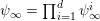










Let us now state more precisely, and prove, two fundamental results ensuring that an LSI holds for canonical measures of the form (1.5).
Theorem 2.10 (Bakry–Emery criterion).
Assume that  ${\mathcal{D}}=\mathbb{R}^{d}$ and
 ${\rm\nabla}^{2}V\geqslant R\,\text{Id}_{d}$ for some constant
 $R>0$. Then
 ${\it\nu}$ satisfies
 $\text{LSI}({\it\beta}R)$.
Proof. The idea is to differentiate the Fisher information with respect to time, in
order to prove its exponential convergence to 0, and then to
insert it in (2.30).
Introduce  $f(t)={\it\psi}(t)/{\it\nu}$ for an arbitrary initial condition
 $f_{0}={\it\psi}_{0}/{\it\nu}$. In view of (2.15), this function evolves according to
 $\partial _{t}f={\mathcal{L}}f$, so that
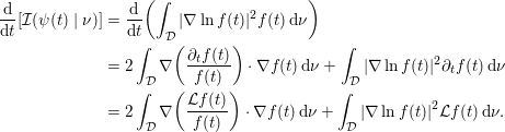 $$\begin{eqnarray}\displaystyle \frac{\text{d}}{\text{d}t}[{\mathcal{I}}({\it\psi}(t)\mid {\it\nu})] & = & \displaystyle \frac{\text{d}}{\text{d}t}\biggl(\int _{{\mathcal{D}}}|{\rm\nabla}\ln f(t)|^{2}f(t)\,\text{d}{\it\nu}\biggr)\nonumber\\ \displaystyle & = & \displaystyle 2\int _{{\mathcal{D}}}{\rm\nabla}\biggl(\displaystyle \frac{\partial _{t}f(t)}{f(t)}\biggr)\cdot {\rm\nabla}f(t)\,\text{d}{\it\nu}+\int _{{\mathcal{D}}}|{\rm\nabla}\ln f(t)|^{2}\partial _{t}f(t)\,\text{d}{\it\nu}\nonumber\\ \displaystyle & = & \displaystyle 2\int _{{\mathcal{D}}}{\rm\nabla}\biggl(\displaystyle \frac{{\mathcal{L}}f(t)}{f(t)}\biggr)\cdot {\rm\nabla}f(t)\,\text{d}{\it\nu}+\int _{{\mathcal{D}}}|{\rm\nabla}\ln f(t)|^{2}{\mathcal{L}}f(t)\,\text{d}{\it\nu}.\nonumber\end{eqnarray}$$
Since
 $$\begin{eqnarray}{\mathcal{L}}(\ln f)=\frac{{\mathcal{L}}f}{f}-\frac{|{\rm\nabla}f|^{2}}{{\it\beta}f^{2}}=\frac{{\mathcal{L}}f}{f}-\frac{1}{{\it\beta}}|{\rm\nabla}(\ln f)|^{2},\end{eqnarray}$$
we obtain, after some algebraic calculations,
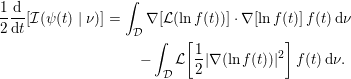 $$\begin{eqnarray}\displaystyle \frac{1}{2}\frac{\text{d}}{\text{d}t}[{\mathcal{I}}({\it\psi}(t)\mid {\it\nu})] & = & \displaystyle \int _{{\mathcal{D}}}{\rm\nabla}[{\mathcal{L}}(\ln f(t))]\cdot {\rm\nabla}[\ln f(t)]\,f(t)\,\text{d}{\it\nu}\nonumber\\ \displaystyle & & \displaystyle \quad -\int _{{\mathcal{D}}}{\mathcal{L}}\biggl[\frac{1}{2}|{\rm\nabla}(\ln f(t))|^{2}\biggr]\,f(t)\,\text{d}{\it\nu}.\nonumber\end{eqnarray}$$
Now, using
 $$\begin{eqnarray}{\rm\nabla}\biggl(\displaystyle \frac{1}{2}|{\rm\nabla}h|^{2}\biggr)={\rm\nabla}^{2}h\cdot {\rm\nabla}h,\quad {\rm\Delta}\biggl(\displaystyle \frac{1}{2}|{\rm\nabla}h|^{2}\biggr)={\rm\nabla}^{2}h:{\rm\nabla}^{2}h+{\rm\nabla}({\rm\Delta}h)\cdot {\rm\nabla}h,\end{eqnarray}$$
it follows that
 $$\begin{eqnarray}\displaystyle {\mathcal{L}}\biggl(\displaystyle \frac{1}{2}|{\rm\nabla}h|^{2}\biggr) & = & \displaystyle \frac{1}{{\it\beta}}({\rm\nabla}^{2}h:{\rm\nabla}^{2}h+{\rm\nabla}({\rm\Delta}h)\cdot {\rm\nabla}h)-({\rm\nabla}V)^{T}({\rm\nabla}^{2}h){\rm\nabla}h\nonumber\\ \displaystyle & {\geqslant} & \displaystyle {\rm\nabla}({\mathcal{L}}h)\cdot {\rm\nabla}h+({\rm\nabla}h)^{T}({\rm\nabla}^{2}V){\rm\nabla}h\nonumber\\ \displaystyle & {\geqslant} & \displaystyle {\rm\nabla}({\mathcal{L}}h)\cdot {\rm\nabla}h+R|{\rm\nabla}h|^{2},\nonumber\end{eqnarray}$$
where we have used  ${\rm\nabla}^{2}h:{\rm\nabla}^{2}h\geqslant 0$ in the second line, and the assumption on
 ${\rm\nabla}^{2}V$ in the third one. We next replace
 $h$ with
 $\ln f(t)$ and obtain
 $$\begin{eqnarray}\frac{1}{2}\frac{\text{d}}{\text{d}t}[{\mathcal{I}}({\it\psi}(t)\mid {\it\nu})]\leqslant -R\int _{{\mathcal{D}}}|{\rm\nabla}(\ln f(t))|^{2}\,f(t)\,\text{d}{\it\nu}=-R\,{\mathcal{I}}({\it\psi}(t)\mid {\it\nu}).\end{eqnarray}$$
This shows that the Fisher information converges exponentially fast to zero:
 $$\begin{eqnarray}{\mathcal{I}}({\it\psi}(t)\mid {\it\nu})\leqslant \text{e}^{-2Rt}{\mathcal{I}}({\it\psi}(0)\mid {\it\nu}).\end{eqnarray}$$
The next step is to prove that  ${\mathcal{H}}({\it\psi}(t,\cdot )\mid {\it\nu})$ converges to 0 as
 $t\rightarrow +\infty$. To this end, we use the argument provided in Arnold
et al. (Reference Arnold, Markowich, Toscani and Unterreiter2001). Since the operator
 $-{\mathcal{L}}$ is self-adjoint on
 $L^{2}({\it\nu})$ and positive by (2.19), its spectral measure
 $P_{{\it\lambda}}$ is supported by
 $[0,+\infty )$; see Reed and Simon (Reference Reed and Simon1975a) and Dautray and Lions (Reference Dautray and Lions1990) for the definition of the spectral
measure. In addition, (2.19) also shows that 0 is a non-degenerate eigenvalue
whose associated eigenvectors are constant functions (recall that since
 ${\it\nu}$ satisfies LSI
 $({\it\beta}R)$,
 ${\it\nu}$ also satisfies a Poincaré inequality with the
same constant: see Proposition 2.12 below). Therefore,
 $$\begin{eqnarray}f(t)=\text{e}^{t{\mathcal{L}}}f_{0}=P_{0}f_{0}+\int _{(0,+\infty )}\text{e}^{-t{\it\lambda}}\,\text{d}(P_{{\it\lambda}}f_{0}).\end{eqnarray}$$
In fact,  $P_{0}$ is the projector onto the eigenspace associated with the
eigenvalue 0, so that
 $P_{0}f_{0}=\int _{{\mathcal{D}}}f_{0}\,\text{d}{\it\nu}=1$. Moreover,
 $$\begin{eqnarray}\Vert f(t)-\mathbf{1}\Vert _{L^{2}({\it\nu})}^{2}=\int _{(0,+\infty )}\text{e}^{-2t{\it\lambda}}\,m_{f_{0}}(\text{d}{\it\lambda}),\quad m_{f_{0}}(\text{d}{\it\lambda})=\text{d}(\Vert P_{{\it\lambda}}f_{0}\Vert _{L^{2}({\it\nu})}^{2}).\end{eqnarray}$$
By dominated convergence, the integral on the right-hand
side of the above equality converges to 0 as  $t\rightarrow +\infty$.
The conclusion now follows by a time integration of (2.30) together with the decay estimate (2.31), which leads to
 $$\begin{eqnarray}{\mathcal{H}}({\it\psi}_{0}\mid {\it\nu})-{\mathcal{H}}({\it\psi}(t,\cdot )\mid {\it\nu})\leqslant \frac{1}{{\it\beta}}\int _{0}^{t}{\mathcal{I}}({\it\psi}(s)\mid {\it\nu})\,\text{d}s\leqslant \frac{1}{2{\it\beta}R}{\mathcal{I}}({\it\psi}_{0}\mid {\it\nu}).\end{eqnarray}$$
In the limit  $t\rightarrow +\infty$, this inequality becomes
 $$\begin{eqnarray}{\mathcal{H}}({\it\psi}_{0}\mid {\it\nu})\leqslant \frac{1}{2{\it\beta}R}{\mathcal{I}}({\it\psi}_{0}\mid {\it\nu}),\end{eqnarray}$$
which gives the claimed LSI since  ${\it\psi}_{0}$ is arbitrary.
Theorem 2.11 (Holley–Stroock).
If  ${\it\nu}$ satisfies
 $\text{LSI}(R)$ and if
 $\widetilde{V}:{\mathcal{D}}\rightarrow \mathbb{R}$ is a bounded function, then
 $\widetilde{{\it\nu}}=\widetilde{Z}^{-1}\,\text{e}^{-\widetilde{V}}{\it\nu}$ satisfies
 $\text{LSI}(\widetilde{R})$ with
 $\widetilde{R}=R\,\text{e}^{\inf \widetilde{V}-\sup \widetilde{V}}$.
Proof. Introduce  ${\it\phi}(x)=x\ln x-1+x$. Consider any function
 $f\geqslant 0$ such that
 $$\begin{eqnarray}\int _{{\mathcal{D}}}f\,\text{d}\widetilde{{\it\nu}}=1,\end{eqnarray}$$
and let  $\overline{f}$ denote the average of
 $f$ with respect to
 ${\it\nu}$:
 $$\begin{eqnarray}\overline{f}=\int _{{\mathcal{D}}}f\,\text{d}{\it\nu}.\end{eqnarray}$$
Then
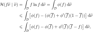 $$\begin{eqnarray}\displaystyle {\mathcal{H}}(f\widetilde{{\it\nu}}\mid \widetilde{{\it\nu}}) & = & \displaystyle \int _{{\mathcal{D}}}f\ln f\,\text{d}\widetilde{{\it\nu}}=\int _{{\mathcal{D}}}{\it\phi}(f)\,\text{d}\widetilde{{\it\nu}}\nonumber\\ \displaystyle & {\leqslant} & \displaystyle \int _{{\mathcal{D}}}[{\it\phi}(f)-({\it\phi}(\overline{f})+{\it\phi}^{\prime }(\overline{f})(1-\overline{f}))]\,\text{d}\widetilde{{\it\nu}}\nonumber\\ \displaystyle & {\leqslant} & \displaystyle \int _{{\mathcal{D}}}[{\it\phi}(f)-{\it\phi}(\overline{f})+{\it\phi}^{\prime }(\overline{f})(\overline{f}-f)]\,\text{d}\widetilde{{\it\nu}},\nonumber\end{eqnarray}$$
since the convexity of  ${\it\phi}$ implies that
 ${\it\phi}(1)=0\geqslant {\it\phi}(\overline{f})+{\it\phi}^{\prime }(\overline{f})(1-\overline{f})$, and where we have used (2.32) to obtain the last line. Note that
 ${\it\phi}(f(q))-{\it\phi}(\overline{f})+{\it\phi}^{\prime }(\overline{f})(\overline{f}-f(q))\geqslant 0$, still by the convexity of
 ${\it\phi}$. Since the integrand is non-negative, we can therefore
reintroduce
 ${\it\nu}$ as follows:
 $$\begin{eqnarray}\displaystyle {\mathcal{H}}(f\widetilde{{\it\nu}}\mid \widetilde{{\it\nu}}) & {\leqslant} & \displaystyle \frac{1}{\widetilde{Z}}\,\text{e}^{-\inf \widetilde{V}}\int _{{\mathcal{D}}}[{\it\phi}(f)-{\it\phi}(\overline{f})+{\it\phi}^{\prime }(\overline{f})(\overline{f}-f)]\,\text{d}{\it\nu}\nonumber\\ \displaystyle & = & \displaystyle \frac{1}{\widetilde{Z}}\,\text{e}^{-\inf \widetilde{V}}\biggl(\int _{{\mathcal{D}}}{\it\phi}(f)\,\text{d}{\it\nu}-{\it\phi}(\overline{f})\biggr),\nonumber\end{eqnarray}$$
in view of (2.33). On the other hand,
 $$\begin{eqnarray}\int _{{\mathcal{D}}}{\it\phi}(f)\,\text{d}{\it\nu}-{\it\phi}(\overline{f})=\int _{{\mathcal{D}}}f\ln f\,\text{d}{\it\nu}-\overline{f}\ln \overline{f}=\overline{f}\int _{{\mathcal{D}}}\frac{f}{\overline{f}}\ln \frac{f}{\overline{f}}\,\text{d}{\it\nu}=\overline{f}\int _{{\mathcal{D}}}{\it\phi}\biggl(\displaystyle \frac{f}{\overline{f}}\biggr)\,\text{d}{\it\nu}.\end{eqnarray}$$
Since  ${\it\nu}$ satisfies LSI(
 $R$), and
 $f/\overline{f}$ has integral 1 with respect to
 ${\it\nu}$,
 $$\begin{eqnarray}\int _{{\mathcal{D}}}{\it\phi}\biggl(\displaystyle \frac{f}{\overline{f}}\biggr)\,\text{d}{\it\nu}\leqslant \frac{1}{2R}\int _{{\mathcal{D}}}\biggl|{\rm\nabla}\ln \biggl(\displaystyle \frac{f}{\overline{f}}\biggr)\biggr|^{2}\biggl(\displaystyle \frac{f}{\overline{f}}\biggr)\,\text{d}{\it\nu}=\frac{1}{2R\overline{f}}\int _{{\mathcal{D}}}|{\rm\nabla}(\ln f)|^{2}f\,\text{d}{\it\nu}.\end{eqnarray}$$
In conclusion,
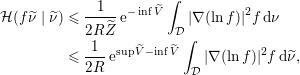 $$\begin{eqnarray}\displaystyle {\mathcal{H}}(f\widetilde{{\it\nu}}\mid \widetilde{{\it\nu}}) & {\leqslant} & \displaystyle \frac{1}{2R\widetilde{Z}}\,\text{e}^{-\inf \widetilde{V}}\int _{{\mathcal{D}}}|{\rm\nabla}(\ln f)|^{2}f\,\text{d}{\it\nu}\nonumber\\ \displaystyle & {\leqslant} & \displaystyle \frac{1}{2R}\,\text{e}^{\sup \widetilde{V}-\inf \widetilde{V}}\int _{{\mathcal{D}}}|{\rm\nabla}(\ln f)|^{2}f\,\text{d}\widetilde{{\it\nu}},\nonumber\end{eqnarray}$$
which gives the claimed statement.
The previous result gives lower bounds on the LSI constants. It suggests that the
LSI constant, and hence the rate of convergence to equilibrium of the overdamped
Langevin dynamics, decreases exponentially as the temperature decreases and/or
energetic barriers increase. Consider for instance the low-temperature regime  ${\it\beta}\rightarrow +\infty$, for a reference convex potential
 $V_{0}(q)=a|q|^{2}/2$ with
 $a>0$, perturbed by a bounded potential
 $\widetilde{V}$, for instance
 $\widetilde{V}(q)=b\exp (-|q|^{2})$ with
 $b>0$. In this case, Theorem 2.10 shows that the canonical measure associated with
 $V$, at inverse temperature
 ${\it\beta}$, satisfies LSI(
 ${\it\beta}a$), while the canonical measure associated with
 $V+\widetilde{V}$, at inverse temperature
 ${\it\beta}$, satisfies LSI(
 ${\it\beta}a\,\text{e}^{-{\it\beta}b}$) by Theorem 2.11. The LSI constants obtained by the Holley–Stroock
perturbative argument are of course lower bounds, but it is indeed expected that
the optimal constant decreases exponentially fast as the temperature decreases
when the potential exhibits energetic barriers. This can be rigorously proved in
one-dimensional systems for example; see Section 2.4 in Menz and
Schlichting (Reference Menz and Schlichting2014).
2.2.3 Relationship between logarithmic Sobolev inequalities and Poincaré inequalities
Initial conditions  ${\it\psi}_{0}$ belonging to
 $L^{2}({\it\nu})$ also have a finite relative entropy with respect to
 ${\it\nu}$. Indeed, using the inequality
 $$\begin{eqnarray}x\ln x-x+1\leqslant (x-1)^{2},\quad \text{for all }x\geqslant 0,\end{eqnarray}$$
it holds that
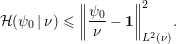 $$\begin{eqnarray}{\mathcal{H}}({\it\psi}_{0}\,|\,{\it\nu})\leqslant \biggl\|\frac{{\it\psi}_{0}}{{\it\nu}}-\mathbf{1}\biggr\|_{L^{2}({\it\nu})}^{2}.\end{eqnarray}$$
This shows that LSIs allow us to cover a larger set of initial conditions than Poincaré inequalities. Unsurprisingly, the following result shows that LSIs are stronger than Poincaré inequalities.
Proposition 2.12 (LSI implies Poincaré inequality).
If a measure  ${\it\nu}$ satisfies an LSI with constant
 $R>0$, then it satisfies a Poincaré inequality with
the same constant.
Proof. The idea of the proof is that the Poincaré inequality can be seen as a linearization of the logarithmic Sobolev inequality. Start from the LSI
 $$\begin{eqnarray}\int _{{\mathcal{D}}}{\it\phi}\ln {\it\phi}\,\text{d}{\it\nu}\leqslant \frac{1}{2R}\int _{{\mathcal{D}}}\frac{|{\rm\nabla}{\it\phi}|^{2}}{{\it\phi}}\,\text{d}{\it\nu},\end{eqnarray}$$
where  ${\it\phi}\geqslant 0$ has average 1 with respect to
 ${\it\nu}$. The function
 ${\it\phi}$ can be chosen of the form
 ${\it\phi}=1+{\it\varepsilon}{\it\varphi}$ where
 ${\it\varphi}\in L^{\infty }({\mathcal{D}})$ has average 0 with respect to
 ${\it\nu}$. For
 $0<{\it\varepsilon}\leqslant 1/(2\Vert {\it\varphi}\Vert _{L^{\infty }})$,
 $$\begin{eqnarray}\int _{{\mathcal{D}}}(1+{\it\varepsilon}{\it\varphi})\ln (1+{\it\varepsilon}{\it\varphi})\,\text{d}{\it\nu}\leqslant \frac{{\it\varepsilon}^{2}}{2R}\int _{{\mathcal{D}}}\frac{|{\rm\nabla}{\it\varphi}|^{2}}{1+{\it\varepsilon}{\it\varphi}}\,\text{d}{\it\nu}=\frac{{\it\varepsilon}^{2}}{2R}\biggl(\int _{{\mathcal{D}}}|{\rm\nabla}{\it\varphi}|^{2}\,\text{d}{\it\nu}+\text{O}({\it\varepsilon})\biggr).\end{eqnarray}$$
Since  $(1+{\it\varepsilon}{\it\varphi})\ln (1+{\it\varepsilon}{\it\varphi})={\it\varepsilon}{\it\varphi}+({\it\varepsilon}{\it\varphi})^{2}+\text{O}({\it\varepsilon}^{3})$, and using the fact that
 ${\it\varphi}$ has average 0 with respect to
 ${\it\nu}$,
 $$\begin{eqnarray}\int _{{\mathcal{D}}}(1+{\it\varepsilon}{\it\varphi})\ln (1+{\it\varepsilon}{\it\varphi})\,\text{d}{\it\nu}={\it\varepsilon}^{2}\biggl(\int _{{\mathcal{D}}}{\it\varphi}^{2}\,\text{d}{\it\nu}+\text{O}({\it\varepsilon})\biggr).\end{eqnarray}$$
The conclusion follows for bounded functions  ${\it\varphi}$ by taking the limit
 ${\it\varepsilon}\rightarrow 0$. The general case can finally be deduced by a density
argument.
2.3 Hypocoercivity
The results from the previous section can be used only for dynamics of overdamped Langevin type, the generators of which are elliptic operators. In this section we provide some methods for the study of convergence to equilibrium of Langevin dynamics (1.9), for which the noise is degenerate since it acts only on the momenta. The generator of Langevin dynamics reads
 $$\begin{eqnarray}{\mathcal{L}}=p^{T}M^{-1}{\rm\nabla}_{q}-{\rm\nabla}V^{T}{\rm\nabla}_{p}+{\it\gamma}\biggl(-p^{T}M^{-1}{\rm\nabla}_{p}+\frac{1}{{\it\beta}}{\rm\Delta}_{p}\biggr),\end{eqnarray}$$
while its adjoint considered on  $L^{2}({\mathcal{E}})$ is
 $$\begin{eqnarray}{\mathcal{L}}^{\dagger }=-p^{T}M^{-1}{\rm\nabla}_{q}+{\rm\nabla}V^{T}{\rm\nabla}_{p}+{\it\gamma}\,\text{div}_{p}\biggl(M^{-1}p\cdot +\frac{1}{{\it\beta}}{\rm\nabla}_{p}\cdot \biggr).\end{eqnarray}$$
Recall that (2.6) shows that the canonical measure
 $$\begin{eqnarray}{\it\mu}(\text{d}q\,\text{d}p)=Z_{{\it\mu}}^{-1}\exp (-{\it\beta}H(q,p))\,\text{d}q\,\text{d}p,\end{eqnarray}$$
where  $H$ is defined in (1.1), is invariant.
2.3.1 Hypoellipticity
Although the generator of the Langevin dynamics and its adjoint are not elliptic,
they can be shown to be hypoelliptic, following the work of
Hörmander Reference Hörmander1967,
Reference Hörmander1985. To this end we introduce the
commutator of two operators  $A,B$:
 $$\begin{eqnarray}[A,B]=AB-BA.\end{eqnarray}$$
We can then state Hörmander’s theorem.
Theorem 2.13. Consider  $C^{\infty }$ vector fields on the
 $D$-dimensional space
 ${\mathcal{Y}}$,
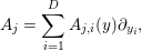 $$\begin{eqnarray}A_{j}=\mathop{\sum }_{i=1}^{D}A_{j,i}(y)\partial _{y_{i}},\end{eqnarray}$$
and introduce the operator
 $$\begin{eqnarray}{\mathcal{A}}=A_{0}+\mathop{\sum }_{j=1}^{J}A_{j}^{\dagger }A_{j},\end{eqnarray}$$
where  $A_{j}^{\dagger }$ is the (formal) adjoint of
 $A_{j}$ on
 $L^{2}({\mathcal{Y}})$. Assume that the Lie algebra spanned by
 $$\begin{eqnarray}\{A_{j}\}_{j=0,\ldots ,J},\quad \{[A_{j},A_{k}]\}_{j,k=0,\ldots ,J},\quad \{[[A_{j},A_{k}],A_{l}]\}_{j,k,l=0,\ldots ,J},\quad \ldots\end{eqnarray}$$
has maximal rank  $D$ at every point
 $y\in {\mathcal{Y}}$. Then
 ${\mathcal{A}}$ is hypoelliptic, namely there exists
 ${\it\varepsilon}>0$ such that
 ${\mathcal{A}}f\in H_{\text{loc}}^{s}$ implies
 $f\in H_{\text{loc}}^{s+{\it\varepsilon}}$.
In particular, solutions  $f$ of the equation
 ${\mathcal{A}}f=0$ are
 $C^{\infty }$.
In order to use this result for Langevin dynamics, we consider  ${\mathcal{Y}}={\mathcal{E}}$,
 $D=2d$,
 $J=d$, and rewrite the generator
 ${\mathcal{L}}$ as
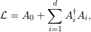 $$\begin{eqnarray}{\mathcal{L}}=A_{0}+\mathop{\sum }_{i=1}^{d}A_{i}^{\dagger }A_{i},\end{eqnarray}$$
with
 $$\begin{eqnarray}A_{0}={\mathcal{L}}_{\text{ham}}-{\it\gamma}p^{T}M^{-1}{\rm\nabla}_{p},\quad A_{i}=\sqrt{\frac{{\it\gamma}}{{\it\beta}}}\partial _{p_{i}}\quad \text{for }1\leqslant i\leqslant d,\end{eqnarray}$$
where
 $$\begin{eqnarray}{\mathcal{L}}_{\text{ham}}=p^{T}M^{-1}{\rm\nabla}_{q}-{\rm\nabla}V^{T}{\rm\nabla}_{p}\end{eqnarray}$$
is the generator of the Hamiltonian part of the dynamics. Assuming
for simplicity that  $M$ is diagonal with entries
 $m_{i}$ (although the computations can be extended to account for
general positive definite mass matrices), we obtain
 $$\begin{eqnarray}[A_{i},A_{0}]{\it\varphi}=\sqrt{\frac{{\it\gamma}}{{\it\beta}}}\frac{1}{m_{i}}(\partial _{q_{i}}-{\it\gamma}\partial _{p_{i}}){\it\varphi}\quad \text{for all }i\in \{1,\ldots ,d\}.\end{eqnarray}$$
Therefore, the Lie algebra generated by  $\{A_{i}\}_{i=1,\ldots ,d}$ and
 $\{[A_{i},A_{0}]\}_{i=1,\ldots ,d}$ has maximal rank
 $2d$ at every configuration
 $(q,p)\in {\mathcal{E}}$. This proves that
 ${\mathcal{L}}$ is hypoelliptic. Similar computations show that
 ${\mathcal{L}}^{\dagger }$ is also hypoelliptic.
Note also that Theorem 2.13 can be used to prove that  $\partial _{t}-{\mathcal{L}}$ and
 $\partial _{t}-{\mathcal{L}}^{\dagger }$ are hypoelliptic on
 ${\mathcal{Y}}=\mathbb{R}\times {\mathcal{E}}$. This ensures that the transition kernel associated with the
Langevin dynamics admits a
 $C^{\infty }$ density (see Section 2.4).
2.3.2 Lack of coercivity on $L_{0}^{2}({\it\mu})$

We recall that we let  ${\mathcal{A}}^{\ast }$ denote the adjoint of a closed operator
 ${\mathcal{A}}$ with respect to the scalar product on
 $L^{2}({\it\mu})$ (see (2.7)). It
turns out to be convenient to rewrite the generator (2.34) as
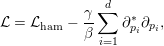 $$\begin{eqnarray}{\mathcal{L}}={\mathcal{L}}_{\text{ham}}-\frac{{\it\gamma}}{{\it\beta}}\mathop{\sum }_{i=1}^{d}\partial _{p_{i}}^{\ast }\partial _{p_{i}},\end{eqnarray}$$
where  $\partial _{p_{i}}^{\ast }={\it\beta}(M^{-1}p)_{i}-\partial _{p_{i}}$. This decomposition highlights an important structural property
of Langevin generators: they are the sum of a Hamiltonian part, and a symmetric
dissipation operator which is degenerate, however, since it acts only on the
momenta. A simple computation shows that the Hamiltonian part is antisymmetric on
 $L^{2}({\it\mu})$, so that the adjoint of
 ${\mathcal{L}}$ on
 $L^{2}({\it\mu})$ reads
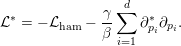 $$\begin{eqnarray}{\mathcal{L}}^{\ast }=-{\mathcal{L}}_{\text{ham}}-\frac{{\it\gamma}}{{\it\beta}}\mathop{\sum }_{i=1}^{d}\partial _{p_{i}}^{\ast }\partial _{p_{i}}.\end{eqnarray}$$
The Fokker–Planck equation (2.1)–(2.3) can be reformulated in terms of
this operator, upon writing  ${\it\psi}(t)=f(t)\,{\it\mu}$, as
 $$\begin{eqnarray}\partial _{t}f={\mathcal{L}}^{\ast }f,\end{eqnarray}$$
where the initial condition  $f(0)=f_{0}={\it\psi}_{0}/{\it\mu}$ satisfies
 $$\begin{eqnarray}f_{0}\geqslant 0,\quad \int _{{\mathcal{E}}}f_{0}\,\text{d}{\it\mu}=1.\end{eqnarray}$$
Note that there is a slight inconsistency in this rewriting: the
initial condition  $f_{0}$ should be considered in
 $L^{1}({\it\mu})$, whereas the functional framework considered here requires the
stronger integrability condition
 $f_{0}\in L^{2}({\it\mu})$. This situation can be improved by using relative
entropies: see Proposition 2.22 below.
In any case,  $\text{e}^{t{\mathcal{L}}^{\ast }}=(\text{e}^{t{\mathcal{L}}})^{\ast }$, so decay estimates obtained for the bounded operator
 $\text{e}^{t{\mathcal{L}}}$ immediately transfer to its adjoint. For simplicity of notation,
the convergence results in Theorems 2.15, 2.18
and Proposition 2.20 are
stated for the semigroup
 $\text{e}^{t{\mathcal{L}}}$, but the reader should bear in mind that the results equally
apply to the semigroup
 $\text{e}^{t{\mathcal{L}}^{\ast }}$, which then yields results on the long-time behaviour of the
Fokker–Planck equation by (2.36).
Note also that solutions to the Fokker–Planck equation (2.36) are expected to converge to
the constant function  $\mathbf{1}$. Upon subtracting this constant function from the initial condition
 $f_{0}$, the convergence of the law amounts to the convergence
to 0 of
 $\text{e}^{t{\mathcal{L}}^{\ast }}(f_{0}-\mathbf{1})$. This motivates the introduction of the following functional
space:
 $$\begin{eqnarray}L_{0}^{2}({\it\mu})=\biggl\{{\it\varphi}\in L^{2}({\it\mu})\,\bigg|\,\int _{{\mathcal{E}}}{\it\varphi}\,\text{d}{\it\mu}=0\biggr\}.\end{eqnarray}$$
The Langevin generator  ${\mathcal{L}}$ defined in (2.34), however, fails to be coercive on
 $L_{0}^{2}({\it\mu})$ since second derivatives in
 $q$ are missing. In fact, for
 $C^{\infty }$ and compactly supported test functions
 ${\it\varphi}$,
 $$\begin{eqnarray}-\langle {\mathcal{L}}{\it\varphi},{\it\varphi}\rangle _{L^{2}({\it\mu})}=\frac{1}{{\it\beta}}\Vert {\rm\nabla}_{p}{\it\varphi}\Vert _{L^{2}({\it\mu})}^{2},\end{eqnarray}$$
which should be compared to (2.19) for overdamped Langevin
dynamics. The key idea of hypocoercivity is to introduce some mixed derivatives in  $q$ and
 $p$ in a modified scalar product in order to retrieve some
dissipation in
 $q$ through some commutator identities. This motivates the name for
the technique, in view of the analogy with hypoellipticity, which allows us, via
certain commutator identities, to state results for non-elliptic operators that
are similar to regularity results obtained for elliptic operators.
More precisely, coercivity is obtained in the Hilbert space  $H^{1}({\it\mu})\cap L_{0}^{2}({\it\mu})$, where
 $$\begin{eqnarray}H^{1}({\it\mu})=\{{\it\varphi}\in L^{2}({\it\mu})\mid {\rm\nabla}_{p}{\it\varphi},{\rm\nabla}_{q}{\it\varphi}\in (L^{2}({\it\mu}))^{d}\}\end{eqnarray}$$
is endowed with a scalar product different from (but equivalent to) the canonical one:
 $$\begin{eqnarray}\langle {\it\varphi}_{1},{\it\varphi}_{2}\rangle _{H^{1}({\it\mu})}=\langle {\it\varphi}_{1},{\it\varphi}_{2}\rangle _{L^{2}({\it\mu})}+\langle {\rm\nabla}_{q}{\it\varphi}_{1},{\rm\nabla}_{q}{\it\varphi}_{2}\rangle _{L^{2}({\it\mu})}+\langle {\rm\nabla}_{p}{\it\varphi}_{1},{\rm\nabla}_{p}{\it\varphi}_{2}\rangle _{L^{2}({\it\mu})}.\end{eqnarray}$$
It is then possible to resort to some Gronwall estimates and
deduce the longtime convergence of  $f(t)$ when a Poincaré inequality holds for
 ${\it\mu}$ (as in the proof of Proposition 2.3).
The idea of using mixed derivatives was already present in the computations
performed in Talay (Reference Talay2002,
Section 3), and was later generalized in Villani (Reference Villani2009). A careful application of the general hypocoercivity
framework to Langevin dynamics can be read in Hairer and Pavliotis (Reference Hairer and Pavliotis2008), where some emphasis is laid on the
limiting regime  ${\it\gamma}\rightarrow 0$; see also Leimkuhler, Matthews and Stoltz (Reference Leimkuhler, Matthews and Stoltz2015) for the regime
 ${\it\gamma}\rightarrow +\infty$.
2.3.3 Estimates in $H^{1}({\it\mu})$

Although hypocoercivity eventually provides decay estimates in  $H^{1}({\it\mu})$, it turns out to be convenient, for the proof, to work with a
specific scalar product equivalent to the canonical scalar product on
 $H^{1}({\it\mu})$. We introduce the following scalar product:
 $$\begin{eqnarray}\langle \!\langle u,v\rangle \!\rangle =\langle u,v\rangle +a\langle {\rm\nabla}_{p}u,{\rm\nabla}_{p}v\rangle -b\langle {\rm\nabla}_{p}u,{\rm\nabla}_{q}v\rangle -b\langle {\rm\nabla}_{q}u,{\rm\nabla}_{p}v\rangle +c\langle {\rm\nabla}_{q}u,{\rm\nabla}_{q}v\rangle ,\end{eqnarray}$$
where, for simplicity of notation, we let  $\langle \cdot ,\cdot \rangle$ denote the standard scalar product on
 $L^{2}({\it\mu})$. In order for the above scalar product to be equivalent to the
canonical scalar product on
 $H^{1}({\it\mu})$, we assume in the remainder of this section that
 $$\begin{eqnarray}a,c>0\quad \text{and}\quad ac-b^{2}>0.\end{eqnarray}$$
Lemma 2.14. Assume that (2.39) holds. Then the bilinear form  $(u,v)\mapsto \langle \!\langle u,v\rangle \!\rangle$ induces a scalar product equivalent to the canonical
scalar product on
 $H^{1}({\it\mu})$.
Proof. Of course,
 $$\begin{eqnarray}|\langle \!\langle u,u\rangle \!\rangle |\leqslant \max (1,a+|b|,c+|b|)\Vert u\Vert _{H^{1}({\it\mu})}^{2}.\end{eqnarray}$$
It therefore remains to prove that  $\Vert u\Vert _{H^{1}({\it\mu})}^{2}$ can be controlled by
 $\langle \!\langle u,u\rangle \!\rangle$. Note first that, by a Cauchy–Schwarz
inequality,
 $$\begin{eqnarray}\displaystyle & & \displaystyle a\langle {\rm\nabla}_{p}u,{\rm\nabla}_{p}u\rangle -b\langle {\rm\nabla}_{p}u,{\rm\nabla}_{q}u\rangle -b\langle {\rm\nabla}_{q}u,{\rm\nabla}_{p}u\rangle +c\langle {\rm\nabla}_{q}u,{\rm\nabla}_{q}u\rangle \nonumber\\ \displaystyle & & \displaystyle \qquad \geqslant \left(\begin{array}{@{}c@{}}\Vert {\rm\nabla}_{p}u\Vert _{L^{2}({\it\mu})}\\ \Vert {\rm\nabla}_{q}u\Vert _{L^{2}({\it\mu})}\end{array}\right)^{T}\left(\begin{array}{@{}cc@{}}a & -|b|\\ -|b| & c\end{array}\right)\left(\begin{array}{@{}c@{}}\Vert {\rm\nabla}_{p}u\Vert _{L^{2}({\it\mu})}\\ \Vert {\rm\nabla}_{q}u\Vert _{L^{2}({\it\mu})}\end{array}\right)\nonumber\\ \displaystyle & & \displaystyle \qquad \geqslant {\it\alpha}(\Vert {\rm\nabla}_{p}u\Vert _{L^{2}({\it\mu})}^{2}+\Vert {\rm\nabla}_{q}u\Vert _{L^{2}({\it\mu})}^{2}),\nonumber\end{eqnarray}$$
where
 $$\begin{eqnarray}{\it\alpha}=\frac{1}{2}(a+c-\sqrt{(a-c)^{2}+4b^{2}})=\displaystyle \frac{2(ac-b^{2})}{a+c+\sqrt{(a-c)^{2}+4b^{2}}}>0.\end{eqnarray}$$
This shows that
 $$\begin{eqnarray}\langle \!\langle u,u\rangle \!\rangle \geqslant \min (1,{\it\alpha})\Vert u\Vert _{H^{1}({\it\mu})}^{2},\end{eqnarray}$$
which allows us to conclude the proof.
As mentioned above, for notational simplicity, we study the convergence
to 0 of  $\text{e}^{t{\mathcal{L}}}{\it\varphi}$ for
 ${\it\varphi}\in L_{0}^{2}({\it\mu})$ rather than the convergence to 0 of
 $\text{e}^{t{\mathcal{L}}^{\ast }}(f_{0}-1)$ for
 $f_{0}\in L^{2}({\it\mu})$. However, the results of this section can be straightforwardly
extended to the latter case by changing the sign of the antisymmetric part of the
operator (which is handled by changing the sign of
 $b$ in the definition of the scalar product
 $\langle \!\langle \cdot ,\cdot \rangle \!\rangle$). The following result can then be stated.
Theorem 2.15 (hypocoercivity).
Fix  ${\it\gamma}>0$, and assume either that the domain
 ${\mathcal{D}}$ is bounded, or that there exists
 ${\it\rho}>0$ such that
 $$\begin{eqnarray}|{\rm\nabla}^{2}V(q)|\leqslant {\it\rho}(1+|{\rm\nabla}V(q)|),\quad \text{for all }q\in {\mathcal{D}},\end{eqnarray}$$
when  ${\mathcal{D}}$ is not bounded. Then there exist
 $a,b,c\in \mathbb{R}$ satisfying (2.39) and
 $K>0$ such that, for any
 ${\it\varphi}\in H^{1}({\it\mu})\cap L_{0}^{2}({\it\mu})$ and any
 $t\geqslant 0$,
 $$\begin{eqnarray}\frac{\text{d}}{\text{d}t}[\langle \!\langle \text{e}^{t{\mathcal{L}}}{\it\varphi},\,\text{e}^{t{\mathcal{L}}}{\it\varphi}\rangle \!\rangle ]\leqslant -K(\Vert {\rm\nabla}_{p}\text{e}^{t{\mathcal{L}}}{\it\varphi}\Vert _{L^{2}({\it\mu})}^{2}+\Vert {\rm\nabla}_{q}\text{e}^{t{\mathcal{L}}}{\it\varphi}\Vert _{L^{2}({\it\mu})}^{2}).\end{eqnarray}$$
Further, if in addition a Poincaré inequality
holds for the measure  ${\it\nu}(\text{d}q)=Z_{{\it\nu}}^{-1}\,\text{e}^{-{\it\beta}V(q)}\,\text{d}q$, then there exists
 ${\it\kappa}>0$ such that, for any
 $t\geqslant 0$,
 $$\begin{eqnarray}\langle \!\langle \text{e}^{t{\mathcal{L}}}{\it\varphi},\,\text{e}^{t{\mathcal{L}}}{\it\varphi}\rangle \!\rangle \leqslant \text{e}^{-2{\it\kappa}t}\langle \!\langle {\it\varphi},{\it\varphi}\rangle \!\rangle ,\quad \text{for all }{\it\varphi}\in H^{1}({\it\mu})\cap L_{0}^{2}({\it\mu}).\end{eqnarray}$$
As a consequence, there exists  $C\geqslant 1$ such that
 $$\begin{eqnarray}\Vert \text{e}^{t{\mathcal{L}}}\Vert _{{\mathcal{B}}(H^{1}({\it\mu})\cap L_{0}^{2}({\it\mu}))}\leqslant C\,\text{e}^{-{\it\kappa}t},\quad \text{for all }t\geqslant 0.\end{eqnarray}$$
In the last inequality,  $H^{1}({\it\mu})$ is endowed with the canonical scalar product. The operator
bound (2.44) is
obtained from (2.43)
by taking the supremum over functions
 ${\it\varphi}\in H^{1}({\it\mu})\cap L_{0}^{2}({\it\mu})$ and using the equivalence of norms provided by
Lemma 2.14. Note that
this implies that
 $C\geqslant 1$.
An immediate consequence of the above convergence result is the following
corollary (obtained from Proposition 2.1 with  $E=H^{1}({\it\mu})\cap L_{0}^{2}({\it\mu})$).
Corollary 2.16. Under the same assumptions as in Theorem 2.15, the operator  ${\mathcal{L}}$ is invertible on
 $H^{1}({\it\mu})\cap L_{0}^{2}({\it\mu})$, and the following equality holds in
 ${\mathcal{B}}(H^{1}({\it\mu})\cap L_{0}^{2}({\it\mu}))$:
 $$\begin{eqnarray}{\mathcal{L}}^{-1}=-\int _{0}^{+\infty }\,\text{e}^{t{\mathcal{L}}}\,\text{d}t.\end{eqnarray}$$
Moreover,
 $$\begin{eqnarray}\Vert {\mathcal{L}}^{-1}\Vert _{{\mathcal{B}}(H^{1}({\it\mu})\cap L_{0}^{2}({\it\mu}))}\leqslant \frac{C}{{\it\kappa}},\end{eqnarray}$$
where  $C$ and
 ${\it\kappa}$ are the same constants as in (2.44).
Let us now present the proof of Theorem 2.15.
Proof. Fix a  $C^{\infty }$ function
 ${\it\varphi}\in H^{1}({\it\mu})\cap L_{0}^{2}({\it\mu})$ (the general case being obtained by a density argument).
Note that
 $$\begin{eqnarray}\frac{\text{d}}{\text{d}t}\biggl(\displaystyle \frac{1}{2}\langle \!\langle \text{e}^{t{\mathcal{L}}}{\it\varphi},\,\text{e}^{t{\mathcal{L}}}{\it\varphi}\rangle \!\rangle \biggr)=\langle \!\langle \text{e}^{t{\mathcal{L}}}{\it\varphi},{\mathcal{L}}\,\text{e}^{t{\mathcal{L}}}{\it\varphi}\rangle \!\rangle .\end{eqnarray}$$
Our aim is to find non-negative constants  $a,b,c$ such that (2.39) holds and, for all
 $C^{\infty }$ functions
 ${\it\varphi}$ with compact support,
 $$\begin{eqnarray}\langle \!\langle {\it\varphi},{\mathcal{L}}{\it\varphi}\rangle \!\rangle \leqslant -{\it\kappa}\langle \!\langle {\it\varphi},{\it\varphi}\rangle \!\rangle .\end{eqnarray}$$
This allows us to obtain (2.42) and thus the desired exponential decrease (2.43), using the
Poincaré inequality and the Gronwall lemma. The idea of
hypocoercivity is thus to find a scalar product equivalent to the canonical  $H^{1}({\it\mu})$ scalar product and such that
 $-{\mathcal{L}}$ is coercive with respect to this scalar product (while it
fails to be coercive with respect to the canonical
 $L^{2}({\it\mu})$ scalar product (see (2.37)), as well as with respect to the canonical
 $H^{1}({\it\mu})$ scalar product).
Let us first compute the various terms in  $\langle \!\langle {\it\varphi},{\mathcal{L}}{\it\varphi}\rangle \!\rangle$. It is useful to first establish some commutator
identities:
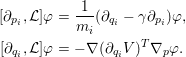 $$\begin{eqnarray}\displaystyle [\partial _{p_{i}},{\mathcal{L}}]{\it\varphi} & = & \displaystyle \frac{1}{m_{i}}(\partial _{q_{i}}-{\it\gamma}\partial _{p_{i}}){\it\varphi},\nonumber\\ \displaystyle [\partial _{q_{i}},{\mathcal{L}}]{\it\varphi} & = & \displaystyle -{\rm\nabla}(\partial _{q_{i}}V)^{T}{\rm\nabla}_{p}{\it\varphi}.\nonumber\end{eqnarray}$$
Some straightforward computations then show that
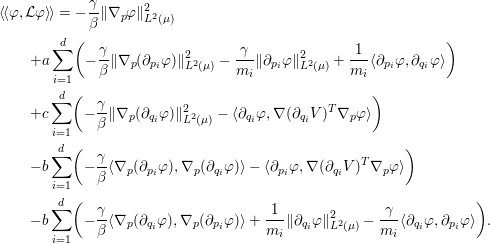 $$\begin{eqnarray}\displaystyle & & \displaystyle \langle \!\langle {\it\varphi},{\mathcal{L}}{\it\varphi}\rangle \!\rangle =-\frac{{\it\gamma}}{{\it\beta}}\Vert {\rm\nabla}_{p}{\it\varphi}\Vert _{L^{2}({\it\mu})}^{2}\nonumber\\ \displaystyle & & \displaystyle \qquad +a\mathop{\sum }_{i=1}^{d}\biggl(-\frac{{\it\gamma}}{{\it\beta}}\Vert {\rm\nabla}_{p}(\partial _{p_{i}}{\it\varphi})\Vert _{L^{2}({\it\mu})}^{2}-\frac{{\it\gamma}}{m_{i}}\Vert \partial _{p_{i}}{\it\varphi}\Vert _{L^{2}({\it\mu})}^{2}+\frac{1}{m_{i}}\langle \partial _{p_{i}}{\it\varphi},\partial _{q_{i}}{\it\varphi}\rangle \biggr)\nonumber\\ \displaystyle & & \displaystyle \qquad +c\mathop{\sum }_{i=1}^{d}\biggl(-\frac{{\it\gamma}}{{\it\beta}}\Vert {\rm\nabla}_{p}(\partial _{q_{i}}{\it\varphi})\Vert _{L^{2}({\it\mu})}^{2}-\langle \partial _{q_{i}}{\it\varphi},{\rm\nabla}(\partial _{q_{i}}V)^{T}{\rm\nabla}_{p}{\it\varphi}\rangle \biggr)\nonumber\\ \displaystyle & & \displaystyle \qquad -b\mathop{\sum }_{i=1}^{d}\biggl(-\frac{{\it\gamma}}{{\it\beta}}\langle {\rm\nabla}_{p}(\partial _{p_{i}}{\it\varphi}),{\rm\nabla}_{p}(\partial _{q_{i}}{\it\varphi})\rangle -\langle \partial _{p_{i}}{\it\varphi},{\rm\nabla}(\partial _{q_{i}}V)^{T}{\rm\nabla}_{p}{\it\varphi}\rangle \biggr)\nonumber\\ \displaystyle & & \displaystyle \qquad -b\mathop{\sum }_{i=1}^{d}\biggl(-\frac{{\it\gamma}}{{\it\beta}}\langle {\rm\nabla}_{p}(\partial _{q_{i}}{\it\varphi}),{\rm\nabla}_{p}(\partial _{p_{i}}{\it\varphi})\rangle +\frac{1}{m_{i}}\Vert \partial _{q_{i}}{\it\varphi}\Vert _{L^{2}({\it\mu})}^{2}-\frac{{\it\gamma}}{m_{i}}\langle \partial _{q_{i}}{\it\varphi},\partial _{p_{i}}{\it\varphi}\rangle \biggr).\nonumber\end{eqnarray}$$
Note in particular that dissipation terms  $\Vert \partial _{q_{i}}{\it\varphi}\Vert _{L^{2}({\it\mu})}^{2}$ appear in the last line. This motivates choosing the
parameter
 $b$ positive.Footnote 6 The next step is to bound the right-hand side of the
previous equality from above using Cauchy–Schwarz inequalities,
by (recall that we assume
 $b\geqslant 0$)
 $$\begin{eqnarray}\displaystyle \langle \!\langle {\it\varphi},{\mathcal{L}}{\it\varphi}\rangle \!\rangle & {\leqslant} & \displaystyle -{\it\gamma}\biggl(\displaystyle \frac{1}{{\it\beta}}+\frac{a}{m_{+}}\biggr)\Vert {\rm\nabla}_{p}{\it\varphi}\Vert _{L^{2}({\it\mu})}^{2}-\frac{b}{m_{+}}\Vert {\rm\nabla}_{q}{\it\varphi}\Vert _{L^{2}({\it\mu})}^{2}\nonumber\\ \displaystyle & & \displaystyle +\frac{a+b{\it\gamma}}{m_{-}}\Vert {\rm\nabla}_{p}{\it\varphi}\Vert _{L^{2}({\it\mu})}\Vert {\rm\nabla}_{q}{\it\varphi}\Vert _{L^{2}({\it\mu})}\nonumber\\ \displaystyle & & \displaystyle -\frac{a{\it\gamma}}{{\it\beta}}\mathop{\sum }_{i=1}^{d}\Vert {\rm\nabla}_{p}(\partial _{p_{i}}{\it\varphi})\Vert _{L^{2}({\it\mu})}^{2}-\frac{c{\it\gamma}}{{\it\beta}}\mathop{\sum }_{i=1}^{d}\Vert {\rm\nabla}_{p}(\partial _{q_{i}}{\it\varphi})\Vert _{L^{2}({\it\mu})}^{2}\nonumber\\ \displaystyle & & \displaystyle +\frac{2b{\it\gamma}}{{\it\beta}}\mathop{\sum }_{i=1}^{d}\Vert {\rm\nabla}_{p}(\partial _{p_{i}}{\it\varphi})\Vert _{L^{2}({\it\mu})}\Vert {\rm\nabla}_{p}(\partial _{q_{i}}{\it\varphi})\Vert _{L^{2}({\it\mu})}\nonumber\\ \displaystyle & & \displaystyle +\langle (b{\rm\nabla}_{p}-c{\rm\nabla}_{q}){\it\varphi},({\rm\nabla}^{2}V){\rm\nabla}_{p}{\it\varphi}\rangle ,\nonumber\end{eqnarray}$$
where
 $$\begin{eqnarray}m_{+}=\max (m_{1},\ldots ,m_{d}),\quad m_{-}=\min (m_{1},\ldots ,m_{d}).\end{eqnarray}$$
Condition (2.39) shows that (by a computation similar to that performed in the proof of Lemma 2.14)
 $$\begin{eqnarray}\displaystyle & & \displaystyle a\Vert {\rm\nabla}_{p}(\partial _{p_{i}}{\it\varphi})\Vert _{L^{2}({\it\mu})}^{2}+c\Vert {\rm\nabla}_{p}(\partial _{q_{i}}{\it\varphi})\Vert _{L^{2}({\it\mu})}^{2}-2b\Vert {\rm\nabla}_{p}(\partial _{p_{i}}{\it\varphi})\Vert _{L^{2}({\it\mu})}\Vert {\rm\nabla}_{p}(\partial _{q_{i}}{\it\varphi})\Vert _{L^{2}({\it\mu})}\nonumber\\ \displaystyle & & \displaystyle \quad \;\geqslant {\it\alpha}(\Vert {\rm\nabla}_{p}(\partial _{p_{i}}{\it\varphi})\Vert _{L^{2}({\it\mu})}^{2}+\Vert {\rm\nabla}_{p}(\partial _{q_{i}}{\it\varphi})\Vert _{L^{2}({\it\mu})}^{2}),\end{eqnarray}$$
with  ${\it\alpha}>0$ defined in (2.40). Therefore, the upper bound on
 $\langle \!\langle {\it\varphi},{\mathcal{L}}{\it\varphi}\rangle \!\rangle$ simplifies as
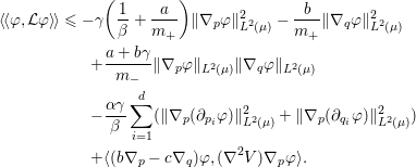 $$\begin{eqnarray}\displaystyle \langle \!\langle {\it\varphi},{\mathcal{L}}{\it\varphi}\rangle \!\rangle & {\leqslant} & \displaystyle -{\it\gamma}\biggl(\displaystyle \frac{1}{{\it\beta}}+\frac{a}{m_{+}}\biggr)\Vert {\rm\nabla}_{p}{\it\varphi}\Vert _{L^{2}({\it\mu})}^{2}-\frac{b}{m_{+}}\Vert {\rm\nabla}_{q}{\it\varphi}\Vert _{L^{2}({\it\mu})}^{2}\nonumber\\ \displaystyle & & \displaystyle \;\;+\frac{a+b{\it\gamma}}{m_{-}}\Vert {\rm\nabla}_{p}{\it\varphi}\Vert _{L^{2}({\it\mu})}\Vert {\rm\nabla}_{q}{\it\varphi}\Vert _{L^{2}({\it\mu})}\nonumber\\ \displaystyle & & \displaystyle \;\;-\frac{{\it\alpha}{\it\gamma}}{{\it\beta}}\mathop{\sum }_{i=1}^{d}(\Vert {\rm\nabla}_{p}(\partial _{p_{i}}{\it\varphi})\Vert _{L^{2}({\it\mu})}^{2}+\Vert {\rm\nabla}_{p}(\partial _{q_{i}}{\it\varphi})\Vert _{L^{2}({\it\mu})}^{2})\nonumber\\ \displaystyle & & \displaystyle \;\;+\langle (b{\rm\nabla}_{p}-c{\rm\nabla}_{q}){\it\varphi},({\rm\nabla}^{2}V){\rm\nabla}_{p}{\it\varphi}\rangle .\end{eqnarray}$$
In order to control the term  $\langle (b{\rm\nabla}_{p}-c{\rm\nabla}_{q}){\it\varphi},({\rm\nabla}^{2}V){\rm\nabla}_{p}{\it\varphi}\rangle$, two cases have to be distinguished.
(i) The position space
${\mathcal{D}}$ is compact. Here ${\rm\nabla}^{2}V$ is uniformly bounded, and there exists a constant $C_{V}>0$ such that $$\begin{eqnarray}\displaystyle & & \displaystyle |\langle (b{\rm\nabla}_{p}-c{\rm\nabla}_{q}){\it\varphi},({\rm\nabla}^{2}V){\rm\nabla}_{p}{\it\varphi}\rangle |\leqslant C_{V}\Vert {\rm\nabla}_{p}{\it\varphi}\Vert _{L^{2}({\it\mu})}\Vert (b{\rm\nabla}_{p}-c{\rm\nabla}_{q}){\it\varphi}\Vert _{L^{2}({\it\mu})}\nonumber\\ \displaystyle & & \displaystyle \qquad \leqslant bC_{V}\Vert {\rm\nabla}_{p}{\it\varphi}\Vert _{L^{2}({\it\mu})}^{2}+cC_{V}\Vert {\rm\nabla}_{p}{\it\varphi}\Vert _{L^{2}({\it\mu})}\Vert {\rm\nabla}_{q}{\it\varphi}\Vert _{L^{2}({\it\mu})}.\nonumber\end{eqnarray}$$(ii) The position space is not compact. Conditions must be imposed on the potential energy function in order to control the growth of the Hessian at infinity. One possible condition is that
${\rm\nabla}^{2}V$ (considered as a multiplication operator acting
on vectors) is relatively bounded by ${\rm\nabla}_{q}$ on $L^{2}({\it\mu})$, that is, there exist $A_{V},B_{V}\geqslant 0$ such that This condition is satisfied when (2.41) holds (see Lemma A.24 of Villani Reference Villani2009). In this case,$$\begin{eqnarray}\forall {\it\phi}\in H^{1}({\it\mu}),\quad \Vert {\it\phi}{\rm\nabla}^{2}V\Vert _{L^{2}({\it\mu})}\leqslant A_{V}\Vert {\it\phi}\Vert _{L^{2}({\it\mu})}+B_{V}\Vert {\rm\nabla}_{q}{\it\phi}\Vert _{L^{2}({\it\mu})}.\end{eqnarray}$$The term involving derivatives in both$$\begin{eqnarray}\displaystyle & & \displaystyle |\langle (b{\rm\nabla}_{p}-c{\rm\nabla}_{q}){\it\varphi},({\rm\nabla}^{2}V){\rm\nabla}_{p}{\it\varphi}\rangle |\nonumber\\ \displaystyle & & \displaystyle \quad \leqslant (A_{V}\Vert {\rm\nabla}_{p}{\it\varphi}\Vert _{L^{2}({\it\mu})}+B_{V}\Vert {\rm\nabla}_{p}{\rm\nabla}_{q}{\it\varphi}\Vert _{L^{2}({\it\mu})})\Vert (b{\rm\nabla}_{p}-c{\rm\nabla}_{q}){\it\varphi}\Vert _{L^{2}({\it\mu})}.\nonumber\end{eqnarray}$$$q$ and $p$ can be controlled by the dissipative terms $-\frac{{\it\alpha}{\it\gamma}}{{\it\beta}}\Vert \partial _{p_{j}}\partial _{q_{i}}{\it\varphi}\Vert _{L^{2}({\it\mu})}^{2}$ in (2.48).







For simplicity, we consider the case when  ${\mathcal{D}}$ is compact. Then,
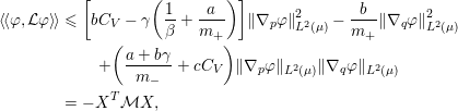 $$\begin{eqnarray}\displaystyle \langle \!\langle {\it\varphi},{\mathcal{L}}{\it\varphi}\rangle \!\rangle & {\leqslant} & \displaystyle \biggl[bC_{V}-{\it\gamma}\biggl(\displaystyle \frac{1}{{\it\beta}}+\frac{a}{m_{+}}\biggr)\biggr]\Vert {\rm\nabla}_{p}{\it\varphi}\Vert _{L^{2}({\it\mu})}^{2}-\frac{b}{m_{+}}\Vert {\rm\nabla}_{q}{\it\varphi}\Vert _{L^{2}({\it\mu})}^{2}\nonumber\\ \displaystyle & & \displaystyle \quad +\biggl(\displaystyle \frac{a+b{\it\gamma}}{m_{-}}+cC_{V}\biggr)\Vert {\rm\nabla}_{p}{\it\varphi}\Vert _{L^{2}({\it\mu})}\Vert {\rm\nabla}_{q}{\it\varphi}\Vert _{L^{2}({\it\mu})}\nonumber\\ \displaystyle & = & \displaystyle -X^{T}{\mathcal{M}}X,\nonumber\end{eqnarray}$$
where
 $$\begin{eqnarray}X=\left(\begin{array}{@{}c@{}}\Vert {\rm\nabla}_{p}{\it\varphi}\Vert _{L^{2}({\it\mu})}\\ \Vert {\rm\nabla}_{q}{\it\varphi}\Vert _{L^{2}({\it\mu})}\end{array}\right)\!,\quad {\mathcal{M}}=\left(\begin{array}{@{}cc@{}}A & C/2\\ C/2 & B\end{array}\right)\!,\end{eqnarray}$$
with
 $$\begin{eqnarray}A={\it\gamma}\biggl(\displaystyle \frac{1}{{\it\beta}}+\frac{a}{m_{+}}\biggr)-bC_{V},\quad B=\frac{b}{m_{+}},\quad C=\frac{a+b{\it\gamma}}{m_{-}}+cC_{V}.\end{eqnarray}$$
In addition to (2.39), the values of  $a,b,c$ should be such that
 $$\begin{eqnarray}4AB>C^{2},\end{eqnarray}$$
in order for  ${\mathcal{M}}$ to be positive definite. If this is the case, (2.42) follows. The
condition (2.49) is satisfied for instance when
 $$\begin{eqnarray}a=c={\it\varepsilon},\quad b={\it\varepsilon}^{1+{\it\delta}},\quad {\it\delta}\in (0,1),\end{eqnarray}$$
for  ${\it\varepsilon}>0$ sufficiently small. Note also that this choice is
compatible with (2.39) when
 ${\it\varepsilon}<1$.
Let us now explain how to get (2.43) from (2.42), assuming that  ${\it\nu}$ satisfies a Poincaré inequality. This requires
us to retrieve some control on the
 $L^{2}({\it\mu})$-norm of
 ${\it\varphi}$ from the norms of the gradient. We use to this end the
fact that, by the tensorization argument stated in
Proposition 2.6,
the canonical measure
 ${\it\mu}$ satisfies a Poincaré inequality, whose constant
we denote by
 $R$. Therefore,
 $X^{T}SX\geqslant \langle \!\langle {\it\varphi},{\it\varphi}\rangle \!\rangle$ with
 $$\begin{eqnarray}S=\left(\begin{array}{@{}cc@{}}a+1/(2R) & -b\\ -b & c+1/(2R)\end{array}\right)\!.\end{eqnarray}$$
We finally define  ${\it\kappa}$ as the largest positive constant such that
 $X^{T}{\mathcal{M}}X\geqslant {\it\kappa}X^{T}SX$. In fact,
 ${\it\kappa}$ is the smallest eigenvalue of
 $S^{-1/2}{\mathcal{M}}S^{-1/2}$ (or equivalently of
 ${\mathcal{M}}S^{-1}$). Since
 $S$ is symmetric positive definite, this shows that
 ${\it\kappa}>0$ since
 ${\mathcal{M}}$ is also positive definite thanks to (2.50). This concludes the
proof of (2.43).
One interest of the hypocoercive approach is that the constants  ${\it\kappa}$ and
 $C$ in (2.44) can be made quite explicit in terms of the various factors (related
to the potential such as the bound on the Hessian
 $C_{V}$ and the Poincaré constant
 $R$, or to the masses). Let us illustrate this for various
asymptotic cases.
(i)
${\it\beta}\rightarrow +\infty$. The constant $R$ typically decreases exponentially with the temperature,
with a lower bound scaling as $\text{e}^{{\it\beta}(\inf \widetilde{V}-\sup \widetilde{V})}$ when $V=V_{\text{convex}}+\widetilde{V}$. In this decomposition, the potential is separated into
a strongly convex part $V_{\text{convex}}$ whose Hessian is uniformly lower bounded by a positive
constant while $\widetilde{V}$ is some bounded perturbation. On the other hand, upon
rescaling the values $a,b,c$ in the definition of the scalar product by a factor $1/{\it\beta}$ (which amounts to considering $a=\overline{a}/{\it\beta}$, etc.), it can be shown that the smallest eigenvalue ${\it\alpha}$ of ${\mathcal{M}}$ is of order $1/{\it\beta}$. Therefore, the smallest eigenvalue ${\it\kappa}$ of $S^{-1/2}{\mathcal{M}}S^{-1/2}$ admits a lower bound which decreases exponentially with ${\it\beta}$.(ii) Hamiltonian limit
${\it\gamma}\rightarrow 0$ or overdamped limit ${\it\gamma}\rightarrow +\infty$. The results stated in Theorem 2.15 are obtained for a given
value of ${\it\gamma}$. On the other hand, the Langevin dynamics becomes
singular in the limit ${\it\gamma}\rightarrow 0$, where it reduces to the Hamiltonian dynamics (which is
not ergodic with respect to the canonical measure), and in the limit ${\it\gamma}\rightarrow +\infty$, where it converges to the overdamped Langevin dynamics
(see the discussion after (1.9)). It is therefore expected that the convergence
rate to equilibrium of the Langevin dynamics degrades as ${\it\gamma}\rightarrow 0$ or ${\it\gamma}\rightarrow +\infty$.Hypocoercivity allows us to quantify the degradation of the convergence rate. Let
${\it\kappa}_{{\it\gamma}}$ denote the exponential decay rate given by
Theorem 2.15
for a given value of ${\it\gamma}$. Upon choosing $(a,b,c)={\it\gamma}(\overline{a},\overline{b},\overline{c})$ when ${\it\gamma}\rightarrow 0$ and $(a,b,c)=(\overline{a},\overline{b},\overline{c})/{\it\gamma}$ when ${\it\gamma}\rightarrow +\infty$, a careful analysis of the scaling of ${\it\kappa}_{{\it\gamma}}$ shows that there exists $\overline{{\it\kappa}}>0$ such that (2.51)The decay rate therefore becomes singular both in the Hamiltonian and overdamped limits. In both cases, the decay is apparent only at long time scales, of order$$\begin{eqnarray}{\it\kappa}_{{\it\gamma}}\geqslant \min \biggl({\it\gamma},\frac{1}{{\it\gamma}}\biggr)\overline{{\it\kappa}}.\end{eqnarray}$$$t/{\it\gamma}$ as ${\it\gamma}\rightarrow 0$ (the fluctuation/dissipation is so small that energy
diffusion is only observed at long times: see Hairer and Pavliotis Reference Hairer and Pavliotis2008 for a precise statement) and ${\it\gamma}t$ as ${\it\gamma}\rightarrow +\infty$ (the fluctuation/dissipation is so large that the
momenta are continuously randomized, which leads to some effective
Brownian motion on the positions over long times). Note however that, for
the limits considered here, the constant $C$ in (2.44) becomes singular. A more convenient
formulation of the scaling limits ${\it\gamma}\rightarrow 0$ or ${\it\gamma}\rightarrow +\infty$ is provided by Proposition 2.20 below.










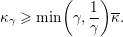


Remark 2.17 (degenerate scalar product).
The standard hypocoercive approach relies on estimates in  $H^{1}({\it\mu})$, obtained under the non-degeneracy condition (2.39). However, in the
situation when
 ${\rm\nabla}^{2}V$ is bounded, it is possible with a slight modification of
the above argumentFootnote 7 to state an exponential convergence in the degenerate
case
 $a=b=c$, for which the associated squared norm is
 $$\begin{eqnarray}\Vert f\Vert _{L^{2}({\it\mu})}^{2}+a\Vert ({\rm\nabla}_{p}-{\rm\nabla}_{q})f\Vert _{L^{2}({\it\mu})}^{2}.\end{eqnarray}$$
2.3.4 Estimates in $L^{2}({\it\mu})$

The passage from bounds in  $H^{1}({\it\mu})$ to bounds in
 $L^{2}({\it\mu})$ follows from hypoelliptic regularization results. Such results
are presented in Villani (Reference Villani2009,
Theorem A.8) or Hairer and Pavliotis (Reference Hairer and Pavliotis2008, Section 6.1). We follow the latter approach, which is
more straightforward, although the so-obtained results are not as strong as the
results presented in Villani (Reference Villani2009).
Theorem 2.18 (hypoelliptic regularization).
Assume  ${\rm\nabla}^{2}V\in L^{\infty }({\mathcal{D}})$ or that (2.41) holds. Then there exists
 $K>0$ such that, for any
 ${\it\varphi}\in L^{2}({\it\mu})$,
 $$\begin{eqnarray}\Vert {\rm\nabla}_{p}\text{e}^{t{\mathcal{L}}}{\it\varphi}\Vert _{L^{2}({\it\mu})}+\Vert {\rm\nabla}_{q}\text{e}^{t{\mathcal{L}}}{\it\varphi}\Vert _{L^{2}({\it\mu})}\leqslant \frac{K}{t^{3/2}}\Vert {\it\varphi}\Vert _{L^{2}({\it\mu})},\quad \text{for all }0<t\leqslant 1.\end{eqnarray}$$
Combining this inequality with  $t=1$ and Theorem 2.15, we can conclude that, for
 $t\geqslant 1$ and
 ${\it\varphi}\in L_{0}^{2}({\it\mu})$,
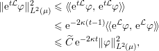 $$\begin{eqnarray}\displaystyle \Vert \text{e}^{t{\mathcal{L}}}{\it\varphi}\Vert _{L^{2}({\it\mu})}^{2} & {\leqslant} & \displaystyle \langle \!\langle \text{e}^{t{\mathcal{L}}}{\it\varphi},\,\text{e}^{t{\mathcal{L}}}{\it\varphi}\rangle \!\rangle \nonumber\\ \displaystyle & {\leqslant} & \displaystyle \text{e}^{-2{\it\kappa}(t-1)}\langle \!\langle \text{e}^{{\mathcal{L}}}{\it\varphi},\,\text{e}^{{\mathcal{L}}}{\it\varphi}\rangle \!\rangle \nonumber\\ \displaystyle & {\leqslant} & \displaystyle \widetilde{C}\,\text{e}^{-2{\it\kappa}t}\Vert {\it\varphi}\Vert _{L^{2}({\it\mu})}^{2},\nonumber\end{eqnarray}$$
which gives an exponential decay in  $L^{2}({\it\mu})$. For completeness, let us recall the proof of
Theorem 2.18, as
presented in Hairer and Pavliotis (Reference Hairer and Pavliotis2008).
Proof. As at the end of the proof of Theorem 2.15, we consider for simplicity the case when  ${\rm\nabla}^{2}V$ is bounded. We denote
 $\text{e}^{t{\mathcal{L}}}{\it\varphi}$ by
 ${\it\varphi}(t)$ in this proof. Define
 $$\begin{eqnarray}\displaystyle N_{{\it\varphi}}(t) & = & \displaystyle \frac{1}{2}[\Vert {\it\varphi}(t)\Vert _{L^{2}({\it\mu})}^{2}+c_{1}t\Vert {\rm\nabla}_{p}{\it\varphi}(t)\Vert _{L^{2}({\it\mu})}^{2}\nonumber\\ \displaystyle & & \displaystyle \quad -c_{2}t^{2}\langle {\rm\nabla}_{q}{\it\varphi}(t),{\rm\nabla}_{p}{\it\varphi}(t)\rangle _{L^{2}({\it\mu})}+c_{3}t^{3}\Vert {\rm\nabla}_{q}{\it\varphi}(t)\Vert _{L^{2}({\it\mu})}^{2}],\end{eqnarray}$$
for some positive constants  $c_{1},c_{2},c_{3}$ to be determined later on. Note that
 $2N_{{\it\varphi}}(t)$ corresponds to the norm induced by the scalar
product (2.38) for time-dependent coefficients
 $a(t)=c_{1}t$,
 $2b(t)=c_{2}t^{2}$ and
 $c(t)=c_{3}t^{3}$. This choice is motivated in Remark 2.19 below. The time derivative
of this quantity reads
 $$\begin{eqnarray}\displaystyle & & \displaystyle \frac{\text{d}N_{{\it\varphi}}(t)}{\text{d}t}=\langle {\it\varphi}(t),{\mathcal{L}}{\it\varphi}(t)\rangle +\frac{c_{1}}{2}\Vert {\rm\nabla}_{p}{\it\varphi}(t)\Vert _{L^{2}({\it\mu})}^{2}+c_{1}t\mathop{\sum }_{i=1}^{d}\langle \partial _{p_{i}}{\it\varphi}(t),\partial _{p_{i}}{\mathcal{L}}{\it\varphi}(t)\rangle \nonumber\\ \displaystyle & & \displaystyle \qquad -c_{2}t\langle {\rm\nabla}_{q}{\it\varphi}(t),{\rm\nabla}_{p}{\it\varphi}(t)\rangle \nonumber\\ \displaystyle & & \displaystyle \qquad -\frac{c_{2}t^{2}}{2}\mathop{\sum }_{i=1}^{d}[\langle \partial _{q_{i}}{\it\varphi}(t),\partial _{p_{i}}{\mathcal{L}}{\it\varphi}(t)\rangle +\langle \partial _{p_{i}}{\it\varphi}(t),\partial _{q_{i}}{\mathcal{L}}{\it\varphi}(t)\rangle ]\nonumber\\ \displaystyle & & \displaystyle \qquad +\frac{3c_{3}t^{2}}{2}\Vert {\rm\nabla}_{q}{\it\varphi}(t)\Vert _{L^{2}({\it\mu})}^{2}+c_{3}t^{3}\mathop{\sum }_{i=1}^{d}\langle \partial _{q_{i}}{\it\varphi}(t),\partial _{q_{i}}{\mathcal{L}}{\it\varphi}(t)\rangle .\nonumber\end{eqnarray}$$
Using computations similar to those in the proof of Theorem 2.15, we obtain
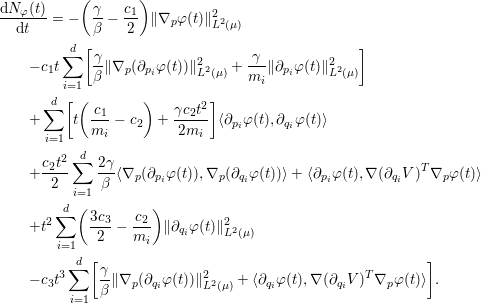 $$\begin{eqnarray}\displaystyle & & \displaystyle \frac{\text{d}N_{{\it\varphi}}(t)}{\text{d}t}=-\biggl(\displaystyle \frac{{\it\gamma}}{{\it\beta}}-\frac{c_{1}}{2}\biggr)\Vert {\rm\nabla}_{p}{\it\varphi}(t)\Vert _{L^{2}({\it\mu})}^{2}\nonumber\\ \displaystyle & & \displaystyle \qquad -c_{1}t\mathop{\sum }_{i=1}^{d}\biggl[\frac{{\it\gamma}}{{\it\beta}}\Vert {\rm\nabla}_{p}(\partial _{p_{i}}{\it\varphi}(t))\Vert _{L^{2}({\it\mu})}^{2}+\frac{{\it\gamma}}{m_{i}}\Vert \partial _{p_{i}}{\it\varphi}(t)\Vert _{L^{2}({\it\mu})}^{2}\biggr]\nonumber\\ \displaystyle & & \displaystyle \qquad +\mathop{\sum }_{i=1}^{d}\biggl[t\biggl(\displaystyle \frac{c_{1}}{m_{i}}-c_{2}\biggr)+\frac{{\it\gamma}c_{2}t^{2}}{2m_{i}}\biggr]\langle \partial _{p_{i}}{\it\varphi}(t),\partial _{q_{i}}{\it\varphi}(t)\rangle \nonumber\\ \displaystyle & & \displaystyle \qquad +\frac{c_{2}t^{2}}{2}\mathop{\sum }_{i=1}^{d}\frac{2{\it\gamma}}{{\it\beta}}\langle {\rm\nabla}_{p}(\partial _{p_{i}}{\it\varphi}(t)),{\rm\nabla}_{p}(\partial _{q_{i}}{\it\varphi}(t))\rangle +\langle \partial _{p_{i}}{\it\varphi}(t),{\rm\nabla}(\partial _{q_{i}}V)^{T}{\rm\nabla}_{p}{\it\varphi}(t)\rangle \nonumber\\ \displaystyle & & \displaystyle \qquad +t^{2}\mathop{\sum }_{i=1}^{d}\biggl(\displaystyle \frac{3c_{3}}{2}-\frac{c_{2}}{m_{i}}\biggr)\Vert \partial _{q_{i}}{\it\varphi}(t)\Vert _{L^{2}({\it\mu})}^{2}\nonumber\\ \displaystyle & & \displaystyle \qquad -c_{3}t^{3}\mathop{\sum }_{i=1}^{d}\biggl[\frac{{\it\gamma}}{{\it\beta}}\Vert {\rm\nabla}_{p}(\partial _{q_{i}}{\it\varphi}(t))\Vert _{L^{2}({\it\mu})}^{2}+\langle \partial _{q_{i}}{\it\varphi}(t),{\rm\nabla}(\partial _{q_{i}}V)^{T}{\rm\nabla}_{p}{\it\varphi}(t)\rangle \biggr].\end{eqnarray}$$
We now choose  $c_{1},c_{2},c_{3}$ such that
 $\text{d}N_{{\it\varphi}}/\text{d}t\leqslant 0$. First, we restrict ourselves to coefficients such that
 $$\begin{eqnarray}c_{2}t^{2}xy\leqslant c_{1}tx^{2}+c_{3}t^{3}y^{2},\quad \text{for all }(x,y)\in \mathbb{R}^{2},\end{eqnarray}$$
which is satisfied once
 $$\begin{eqnarray}c_{1},c_{3}\geqslant 0,\quad 4c_{1}c_{3}\geqslant c_{2}^{2}.\end{eqnarray}$$
Then,
 $$\begin{eqnarray}\displaystyle -c_{1}t\mathop{\sum }_{i=1}^{d}\frac{{\it\gamma}}{{\it\beta}}\Vert {\rm\nabla}_{p}(\partial _{p_{i}}{\it\varphi}(t))\Vert _{L^{2}({\it\mu})}^{2}+\frac{c_{2}t^{2}}{2}\mathop{\sum }_{i=1}^{d}\frac{2{\it\gamma}}{{\it\beta}}\langle {\rm\nabla}_{p}(\partial _{p_{i}}{\it\varphi}(t)),{\rm\nabla}_{p}(\partial _{q_{i}}{\it\varphi}(t))\rangle & & \displaystyle \nonumber\\ \displaystyle -c_{3}t^{3}\mathop{\sum }_{i=1}^{d}\frac{{\it\gamma}}{{\it\beta}}\Vert {\rm\nabla}_{p}(\partial _{q_{i}}{\it\varphi}(t))\Vert _{L^{2}({\it\mu})}^{2}\leqslant 0, & & \displaystyle \nonumber\end{eqnarray}$$
so that, with  $C_{V}=\Vert {\rm\nabla}^{2}V\Vert _{L^{\infty }}$,
 $$\begin{eqnarray}\displaystyle & & \displaystyle \frac{\text{d}N_{{\it\varphi}}(t)}{\text{d}t}\leqslant -\biggl(\displaystyle \frac{{\it\gamma}}{{\it\beta}}+\frac{{\it\gamma}c_{1}t}{m_{+}}-\frac{c_{1}}{2}-C_{V}\frac{c_{2}t^{2}}{2}\biggr)\Vert {\rm\nabla}_{p}{\it\varphi}(t)\Vert _{L^{2}({\it\mu})}^{2}\nonumber\\ \displaystyle & & \displaystyle \qquad -t^{2}\biggl(\displaystyle \frac{c_{2}}{m_{+}}-\frac{3c_{3}}{2}\biggr)\Vert {\rm\nabla}_{q}{\it\varphi}(t)\Vert _{L^{2}({\it\mu})}^{2}\nonumber\\ \displaystyle & & \displaystyle \qquad +\biggl[t\biggl(\displaystyle \frac{c_{1}}{m_{-}}-c_{2}\biggr)+\frac{{\it\gamma}c_{2}t^{2}}{2m_{-}}+C_{V}c_{3}t^{3}\biggr]\Vert {\rm\nabla}_{p}{\it\varphi}(t)\Vert _{L^{2}({\it\mu})}\Vert {\rm\nabla}_{q}{\it\varphi}(t)\Vert _{L^{2}({\it\mu})}.\nonumber\end{eqnarray}$$
On the time interval  $[0,1]$, we finally obtain the following upper bound:
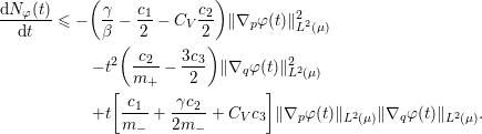 $$\begin{eqnarray}\displaystyle \frac{\text{d}N_{{\it\varphi}}(t)}{\text{d}t} & {\leqslant} & \displaystyle -\biggl(\displaystyle \frac{{\it\gamma}}{{\it\beta}}-\frac{c_{1}}{2}-C_{V}\frac{c_{2}}{2}\biggr)\Vert {\rm\nabla}_{p}{\it\varphi}(t)\Vert _{L^{2}({\it\mu})}^{2}\nonumber\\ \displaystyle & & \displaystyle \quad -t^{2}\biggl(\displaystyle \frac{c_{2}}{m_{+}}-\frac{3c_{3}}{2}\biggr)\Vert {\rm\nabla}_{q}{\it\varphi}(t)\Vert _{L^{2}({\it\mu})}^{2}\nonumber\\ \displaystyle & & \displaystyle \quad +t\biggl[\frac{c_{1}}{m_{-}}+\frac{{\it\gamma}c_{2}}{2m_{-}}+C_{V}c_{3}\biggr]\Vert {\rm\nabla}_{p}{\it\varphi}(t)\Vert _{L^{2}({\it\mu})}\Vert {\rm\nabla}_{q}{\it\varphi}(t)\Vert _{L^{2}({\it\mu})}.\nonumber\end{eqnarray}$$
We next consider coefficients  $c_{3}\ll c_{2}\ll c_{1}\ll 1$ satisfying (2.54) and
 $c_{1}^{2}\ll c_{2}$. For instance,
 $c_{1}={\it\varepsilon}$,
 $c_{2}={\it\varepsilon}^{1+{\it\delta}}$ and
 $c_{3}={\it\varepsilon}^{1+{\it\delta}+{\it\eta}}$, with
 $0<{\it\eta}<{\it\delta}<1$ and for
 ${\it\varepsilon}>0$ sufficiently small. We can then deduce that
 $\text{d}N_{{\it\varphi}}(t)/\text{d}t\leqslant 0$, which implies
 $N_{{\it\varphi}}(t)\leqslant N_{{\it\varphi}}(0)=\Vert {\it\varphi}\Vert _{L^{2}({\it\mu})}^{2}/2$. The desired conclusion immediately follows.
Remark 2.19. Let us now motivate definition (2.52) more precisely. As discussed after this equation, the
choice (2.52) corresponds
to the scalar product (2.38) with time-dependent coefficients  $a(t),b(t),c(t)$. First, in order to only have the
 $L^{2}({\it\mu})$-norm of
 ${\it\varphi}$ at time
 $t=0$ in
 $N_{{\it\varphi}}(0)$, it is necessary that
 $a(0)=b(0)=c(0)=0$. Second, when generalizing the computations leading to
(2.53), the prefactors
of the third and fifth terms on the right-hand side of (2.53) now read
 $a(t)/m_{i}-b^{\prime }(t)+{\it\gamma}b(t)/m_{i}$ instead of
 $t(c_{1}/m_{i}-c_{2})+{\it\gamma}c_{2}t^{2}/(2m_{i})$ and
 $c^{\prime }(t)/2-2b(t)/m_{i}$ instead of
 $t^{2}(3c_{3}/2-c_{2}/m_{i})$. This suggests that
 $a(t)$ and
 $b^{\prime }(t)$ should be of the same order of magnitude, as well as
 $b(t)$ and
 $c^{\prime }(t)$. When
 $a(t)$ is linear in
 $t$, this implies that
 $b(t)$ is quadratic and
 $c(t)$ cubic.
By tracking the dependency of the constant  $K$ on
 ${\it\gamma}$, Theorem 2.18 combined with Theorem 2.15 and the estimate (2.51) leads to the following result.
Proposition 2.20. Assume that  ${\rm\nabla}^{2}V\in L^{\infty }({\mathcal{D}})$ and that a Poincaré inequality holds for
 ${\it\nu}$. Then there exist
 $C,\overline{{\it\kappa}}>0$ such that, for all
 ${\it\gamma}>0$, for all
 ${\it\varphi}\in L_{0}^{2}({\it\mu})$,
 $$\begin{eqnarray}\Vert \text{e}^{t{\mathcal{L}}}{\it\varphi}\Vert _{L^{2}({\it\mu})}\leqslant C\,\text{e}^{-\overline{{\it\kappa}}\min ({\it\gamma},{\it\gamma}^{-1})t}\Vert {\it\varphi}\Vert _{L^{2}({\it\mu})}.\end{eqnarray}$$
This result again emphasizes the fact that, in the limiting regimes of very low or
very large frictions, the system should be considered over long times  $\max ({\it\gamma},1/{\it\gamma})t$ in order to display a non-trivial behaviour.
Similarly to Corollary 2.16, the following result can be stated.
Corollary 2.21. Under the same assumptions as in Proposition 2.20, the operator  ${\mathcal{L}}$ is invertible on
 $L_{0}^{2}({\it\mu})$, and the equality
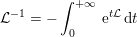 $$\begin{eqnarray}{\mathcal{L}}^{-1}=-\int _{0}^{+\infty }\,\text{e}^{t{\mathcal{L}}}\,\text{d}t\end{eqnarray}$$
holds in  ${\mathcal{B}}(L_{0}^{2}({\it\mu}))$. Moreover,
 $$\begin{eqnarray}\Vert {\mathcal{L}}^{-1}\Vert _{{\mathcal{B}}(L_{0}^{2}({\it\mu}))}\leqslant \frac{C}{\overline{{\it\kappa}}\min ({\it\gamma},{\it\gamma}^{-1})},\end{eqnarray}$$
where  $C$ and
 $\overline{{\it\kappa}}$ are the same constants as in (2.55).
2.3.5 Hypocoercivity in the entropic sense
Here we show how the computations performed in  $H^{1}({\it\mu})$ can be modified to prove the decay of some logarithmic entropy,
similar to the one used for LSIs. The interest of this approach is that initial
conditions in larger functional spaces can be considered. The general strategy is
presented in Villani (Reference Villani2009,
Section 6). These computations can be simplified for Langevin-type
dynamics: see Olla and Letizia (Reference Olla and Letizia2015, Appendix D).
We state here convergence results for the function  $f(t)$, which is the Radon–Nikodym derivative of the law
 ${\it\psi}(t)$ of the process at time
 $t$ with respect to the density of the invariant measure
 ${\it\mu}$. Starting from
 $f_{0}\geqslant 0$ with
 $\int _{{\mathcal{E}}}f_{0}\,\text{d}{\it\mu}=1$, the function
 $f(t)$ therefore evolves according to the Fokker–Planck
equation (2.36), that is,
 $f(t)=\text{e}^{t{\mathcal{L}}^{\ast }}f_{0}$. It is expected that
 $f(t)$ converges to the constant function
 $\mathbf{1}$.
To quantify the convergence rate, we introduce the entropy functional
 $$\begin{eqnarray}\mathscr{E}(f)=\int _{{\mathcal{E}}}f\,\ln f\,\text{d}{\it\mu}+\int _{{\mathcal{E}}}\frac{{\rm\nabla}f^{T}S{\rm\nabla}f}{f}\,\text{d}{\it\mu},\end{eqnarray}$$
where  $S\in \mathbb{R}^{2d\times 2d}$ is a non-negative symmetric matrix. Note that the functional
 $\mathscr{E}$ combines the relative entropy and a generalization of the Fisher
information introduced in Definition 2.7. It is sufficient for our purposes to restrict
ourselves to the case when
 $S$ is constant (but see Villani Reference Villani2009, Remark 29 for a context where a dependence on the
position
 $q$ may be useful). Finally, note that
 $\mathscr{E}(\mathbf{1})=0$, so that the entropy is expected to converge to 0 as
 $t\rightarrow +\infty$.
Proposition 2.22. Assume  ${\rm\nabla}^{2}V\in L^{\infty }({\mathcal{D}})$. Then there exist a non-negative symmetric matrix
 $S\in \mathbb{R}^{2d\times 2d}$ and
 ${\it\alpha}>0$ such that
 $$\begin{eqnarray}\frac{\text{d}}{\text{d}t}[\mathscr{E}(f(t))]\leqslant -{\it\alpha}\int _{{\mathcal{E}}}\frac{|{\rm\nabla}f(t)|^{2}}{f(t)}\,\text{d}{\it\mu},\quad \text{for all }t\geqslant 0.\end{eqnarray}$$
If in addition  ${\it\nu}(\text{d}q)$ satisfies a logarithmic Sobolev inequality, then there
exists
 ${\it\kappa}>0$ such that
 $$\begin{eqnarray}\frac{\text{d}}{\text{d}t}[\mathscr{E}(f(t))]\leqslant -{\it\kappa}\,\mathscr{E}(f(t)),\quad \text{for all }t\geqslant 0.\end{eqnarray}$$
In particular,  $0\leqslant \mathscr{E}(f(t))\leqslant \mathscr{E}(f_{0})\,\text{e}^{-{\it\kappa}t}$ for any
 $t\geqslant 0$.
Notice that we do not require the matrix  $S$ to be definite for the result to hold.
Proof. One of the main ideas in the proof is to rewrite the time derivative of the
second term in the expression of  $\mathscr{E}$ as a sum of terms similar to the ones appearing in the
proof of Theorem 2.15. To this end, consider
 $g(t)=\sqrt{f(t)}$, so that
 $$\begin{eqnarray}\int _{{\mathcal{E}}}\frac{{\rm\nabla}f(t)^{T}S{\rm\nabla}f(t)}{f(t)}\,\text{d}{\it\mu}=4\int _{{\mathcal{E}}}{\rm\nabla}g(t)^{T}S{\rm\nabla}g(t)\,\text{d}{\it\mu}.\end{eqnarray}$$
In order to determine the time evolution of this quantity,
we first write the time evolution for  $g(t)$. Simple computations show that
 $$\begin{eqnarray}\displaystyle \partial _{t}g(t) & = & \displaystyle \frac{\partial _{t}f(t)}{2\sqrt{f(t)}}=\frac{{\mathcal{L}}^{\ast }f(t)}{2g(t)},\nonumber\\ \displaystyle {\rm\Delta}_{p}g(t) & = & \displaystyle \frac{{\rm\Delta}_{p}f(t)}{2\sqrt{f(t)}}-\frac{|{\rm\nabla}_{p}f(t)|^{2}}{4f(t)^{3/2}}=\frac{{\rm\Delta}_{p}f(t)}{2g(t)}-\frac{|{\rm\nabla}_{p}g(t)|^{2}}{g(t)},\nonumber\end{eqnarray}$$
so that
 $$\begin{eqnarray}\partial _{t}g(t)={\mathcal{L}}^{\ast }g(t)+\frac{{\it\gamma}}{{\it\beta}}\frac{|{\rm\nabla}_{p}g(t)|^{2}}{g(t)}.\end{eqnarray}$$
We next compute the time derivatives of the various terms in  $\mathscr{E}(f(t))$, relying on the reformulation (2.59). This leads to
expressions very similar to those encountered in the proof of
Theorem 2.15.
First,
 $$\begin{eqnarray}\displaystyle & & \displaystyle \frac{\text{d}}{\text{d}t}\biggl(\int _{{\mathcal{E}}}f(t)\,\ln f(t)\,\text{d}{\it\mu}\biggr)=\int _{{\mathcal{E}}}(1+\ln f(t)){\mathcal{L}}^{\ast }f(t)\,\text{d}{\it\mu}\nonumber\\ \displaystyle & & \displaystyle \qquad =\int _{{\mathcal{E}}}{\mathcal{L}}_{\text{ham}}(1+\ln f(t))f(t)\,\text{d}{\it\mu}-\frac{{\it\gamma}}{{\it\beta}}\int _{{\mathcal{E}}}{\rm\nabla}_{p}f(t)\cdot {\rm\nabla}_{p}(\ln f(t))\,\text{d}{\it\mu}\nonumber\\ \displaystyle & & \displaystyle \qquad =\int _{{\mathcal{E}}}{\mathcal{L}}_{\text{ham}}f(t)\,\text{d}{\it\mu}-\frac{{\it\gamma}}{{\it\beta}}\int _{{\mathcal{E}}}\frac{|{\rm\nabla}_{p}f(t)|^{2}}{f(t)}\,\text{d}{\it\mu}=-\frac{4{\it\gamma}}{{\it\beta}}\int _{{\mathcal{E}}}|{\rm\nabla}_{p}g(t)|^{2}\,\text{d}{\it\mu},\nonumber\end{eqnarray}$$
in view of the invariance of  ${\it\mu}$ by
 ${\mathcal{L}}_{\text{ham}}$. Next,
 $$\begin{eqnarray}\displaystyle & & \displaystyle \frac{\text{d}}{\text{d}t}\biggl(\int _{{\mathcal{E}}}|\partial _{p_{i}}g(t)|^{2}\,\text{d}{\it\mu}\biggr)=2\int _{{\mathcal{E}}}\partial _{p_{i}}g(t)\,\partial _{p_{i}}({\mathcal{L}}^{\ast }g(t))\,\text{d}{\it\mu}\nonumber\\ \displaystyle & & \displaystyle \qquad \qquad +\frac{2{\it\gamma}}{{\it\beta}}\!\int _{{\mathcal{E}}}\partial _{p_{i}}g(t)\,\partial _{p_{i}}\biggl(\displaystyle \frac{|{\rm\nabla}_{p}g(t)|^{2}}{g(t)}\biggr)\,\text{d}{\it\mu}\nonumber\\ \displaystyle & & \displaystyle \qquad =2\int _{{\mathcal{E}}}\partial _{p_{i}}g(t)\,{\mathcal{L}}^{\ast }(\partial _{p_{i}}g(t))\,\text{d}{\it\mu}-\frac{2}{m_{i}}\int _{{\mathcal{E}}}\partial _{p_{i}}g(t)\,(\partial _{q_{i}}+{\it\gamma}\partial _{p_{i}})g(t)\,\text{d}{\it\mu}\nonumber\\ \displaystyle & & \displaystyle \qquad \qquad +\frac{2{\it\gamma}}{{\it\beta}}\int _{{\mathcal{E}}}\partial _{p_{i}}g(t)\biggl(\displaystyle \frac{2{\rm\nabla}_{p}(\partial _{p_{i}}g(t)){\rm\nabla}_{p}g(t)}{g(t)}-\frac{|{\rm\nabla}_{p}g(t)|^{2}}{g(t)^{2}}\partial _{p_{i}}g(t)\biggr)\,\text{d}{\it\mu}\nonumber\\ \displaystyle & & \displaystyle \qquad =-\frac{2}{m_{i}}\int _{{\mathcal{E}}}\partial _{p_{i}}g(t)\,(\partial _{q_{i}}+{\it\gamma}\partial _{p_{i}})g(t)\,\text{d}{\it\mu}\nonumber\\ \displaystyle & & \displaystyle \qquad \qquad -\frac{2{\it\gamma}}{{\it\beta}}\int _{{\mathcal{E}}}|{\rm\nabla}_{p}\partial _{p_{i}}g(t)|^{2}-2{\rm\nabla}_{p}(\partial _{p_{i}}g(t))\cdot \frac{(\partial _{p_{i}}g(t)){\rm\nabla}_{p}g(t)}{g(t)}\,\text{d}{\it\mu}\nonumber\\ \displaystyle & & \displaystyle \qquad \qquad -\,\displaystyle \frac{2{\it\gamma}}{{\it\beta}}\int _{{\mathcal{E}}}\frac{|{\rm\nabla}_{p}g(t)|^{2}(\partial _{p_{i}}g(t))^{2}}{g(t)^{2}}\,\text{d}{\it\mu},\nonumber\\ \displaystyle & & \displaystyle \nonumber\end{eqnarray}$$
where we have used
 $$\begin{eqnarray}\displaystyle \int _{{\mathcal{E}}}\partial _{p_{i}}g(t)\,{\mathcal{L}}^{\ast }(\partial _{p_{i}}g(t))\,\text{d}{\it\mu} & = & \displaystyle -\int _{{\mathcal{E}}}\partial _{p_{i}}g(t)\,{\mathcal{L}}_{\text{ham}}(\partial _{p_{i}}g(t))\,\text{d}{\it\mu}\nonumber\\ \displaystyle & & \displaystyle \quad -\frac{2{\it\gamma}}{{\it\beta}}\mathop{\sum }_{j=1}^{d}\int _{{\mathcal{E}}}\partial _{p_{i}}g(t)\,\partial _{p_{j}}^{\ast }\partial _{p_{j}}(\partial _{p_{i}}g(t))\,\text{d}{\it\mu},\nonumber\end{eqnarray}$$
and the first integral on the right-hand side vanishes since  ${\mathcal{L}}_{\text{ham}}$ is antisymmetric. Therefore,
 $$\begin{eqnarray}\displaystyle \frac{\text{d}}{\text{d}t}\biggl(\int _{{\mathcal{E}}}|\partial _{p_{i}}g(t)|^{2}\,\text{d}{\it\mu}\biggr) & = & \displaystyle -\frac{2}{m_{i}}\int _{{\mathcal{E}}}\partial _{p_{i}}g(t)\,(\partial _{q_{i}}+{\it\gamma}\partial _{p_{i}})g(t)\,\text{d}{\it\mu}\nonumber\\ \displaystyle & & \displaystyle \quad -\frac{2{\it\gamma}}{{\it\beta}}\int _{{\mathcal{E}}}\biggl|{\rm\nabla}_{p}\partial _{p_{i}}g(t)-\frac{(\partial _{p_{i}}g(t)){\rm\nabla}_{p}g(t)}{g(t)}\biggr|^{2}\,\text{d}{\it\mu}.\nonumber\end{eqnarray}$$
Similar computations give
 $$\begin{eqnarray}\displaystyle \frac{\text{d}}{\text{d}t}\biggl(\int _{{\mathcal{E}}}|\partial _{q_{i}}g(t)|^{2}\,\text{d}{\it\mu}\biggr) & = & \displaystyle 2\int _{{\mathcal{E}}}\partial _{q_{i}}g(t)\,({\rm\nabla}\partial _{q_{i}}V)\cdot {\rm\nabla}_{p}g(t)\,\text{d}{\it\mu}\nonumber\\ \displaystyle & & \displaystyle \quad -\frac{2{\it\gamma}}{{\it\beta}}\int _{{\mathcal{E}}}\biggl|{\rm\nabla}_{p}\partial _{q_{i}}g(t)-\frac{(\partial _{q_{i}}g(t)){\rm\nabla}_{p}g(t)}{g(t)}\biggr|^{2}\,\text{d}{\it\mu},\nonumber\end{eqnarray}$$
and
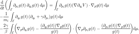 $$\begin{eqnarray}\displaystyle & & \displaystyle \frac{\text{d}}{\text{d}t}\biggl(\int _{{\mathcal{E}}}\partial _{p_{i}}g(t)\,\partial _{q_{i}}g(t)\,\text{d}{\it\mu}\biggr)=\int _{{\mathcal{E}}}\partial _{p_{i}}g(t)({\rm\nabla}\partial _{q_{i}}V)\cdot {\rm\nabla}_{p}g(t)\,\text{d}{\it\mu}\nonumber\\ \displaystyle & & \displaystyle -\frac{1}{m_{i}}\int _{{\mathcal{E}}}\partial _{q_{i}}g(t)\,(\partial _{q_{i}}+{\it\gamma}\partial _{p_{i}})g(t)\,\text{d}{\it\mu}\nonumber\\ \displaystyle & & \displaystyle -\frac{2{\it\gamma}}{{\it\beta}}\int _{{\mathcal{E}}}\biggl(\!{\rm\nabla}_{p}\partial _{q_{i}}g(t)-\frac{(\partial _{q_{i}}g(t)){\rm\nabla}_{p}g(t)}{g(t)}\!\biggr)\cdot \biggl(\!{\rm\nabla}_{p}\partial _{p_{i}}g(t)-\frac{(\partial _{p_{i}}g(t)){\rm\nabla}_{p}g(t)}{g(t)}\!\biggr)\text{d}{\it\mu}.\nonumber\end{eqnarray}$$
Considering
 $$\begin{eqnarray}S=\left(\begin{array}{@{}cc@{}}a\,\text{Id}_{d} & b\,\text{Id}_{d}\\ b\,\text{Id}_{d} & c\,\text{Id}_{d}\end{array}\right)\!,\end{eqnarray}$$
it follows that
 $$\begin{eqnarray}\frac{\text{d}}{\text{d}t}(\mathscr{E}(f(t)))=-\frac{4{\it\gamma}}{{\it\beta}}\int _{{\mathcal{E}}}|{\rm\nabla}_{p}g(t)|^{2}\,\text{d}{\it\mu}+\mathop{\sum }_{i=1}^{d}\int _{{\it\varepsilon}}U_{i}(t)\,\text{d}{\it\mu},\end{eqnarray}$$
where
 $$\begin{eqnarray}\displaystyle & & \displaystyle U_{i}(t)=8a\partial _{q_{i}}g(t)\,({\rm\nabla}\partial _{q_{i}}V)\cdot {\rm\nabla}_{p}g(t)\nonumber\\ \displaystyle & & \displaystyle \;\;-8b\biggl(-\partial _{p_{i}}g(t)\,({\rm\nabla}\partial _{q_{i}}V)\cdot {\rm\nabla}_{p}g(t)+\frac{1}{m_{i}}\partial _{q_{i}}g(t)\,(\partial _{q_{i}}+{\it\gamma}\partial _{p_{i}})g(t)\biggr)\nonumber\\ \displaystyle & & \displaystyle \;\;-\frac{8c}{m_{i}}\partial _{p_{i}}g(t)\,(\partial _{q_{i}}+{\it\gamma}\partial _{p_{i}})g(t)\nonumber\\ \displaystyle & & \displaystyle -\frac{8{\it\gamma}a}{{\it\beta}}\biggl|{\rm\nabla}_{p}\partial _{q_{i}}g(t)-\frac{(\partial _{q_{i}}g(t)){\rm\nabla}_{p}g(t)}{g(t)}\biggr|^{2}\nonumber\\ \displaystyle & & \displaystyle \;\;-\frac{16{\it\gamma}b}{{\it\beta}}\biggl({\rm\nabla}_{p}\partial _{q_{i}}g(t)-\frac{(\partial _{q_{i}}g(t)){\rm\nabla}_{p}g(t)}{g(t)}\biggr)\cdot \biggl({\rm\nabla}_{p}\partial _{p_{i}}g(t)-\frac{(\partial _{p_{i}}g(t)){\rm\nabla}_{p}g(t)}{g(t)}\biggr)\nonumber\\ \displaystyle & & \displaystyle \;\;-\frac{8{\it\gamma}c}{{\it\beta}}\biggl|{\rm\nabla}_{p}\partial _{p_{i}}g(t)-\frac{(\partial _{p_{i}}g(t)){\rm\nabla}_{p}g(t)}{g(t)}\biggr|^{2}.\nonumber\end{eqnarray}$$
Note that the sum of the last three terms in  $U_{i}(t)$, integrated against
 ${\it\mu}$, can be bounded from above by
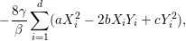 $$\begin{eqnarray}-\frac{8{\it\gamma}}{{\it\beta}}\mathop{\sum }_{i=1}^{d}(aX_{i}^{2}-2bX_{i}Y_{i}+cY_{i}^{2}),\end{eqnarray}$$
with
 $$\begin{eqnarray}\displaystyle X_{i} & = & \displaystyle \biggl\|{\rm\nabla}_{p}\partial _{q_{i}}g(t)-\displaystyle \frac{(\partial _{q_{i}}g(t)){\rm\nabla}_{p}g(t)}{g(t)}\biggr\|_{L^{2}({\it\mu})},\nonumber\\ \displaystyle Y_{i} & = & \displaystyle \biggl\|{\rm\nabla}_{p}\partial _{p_{i}}g(t)-\displaystyle \frac{(\partial _{p_{i}}g(t)){\rm\nabla}_{p}g(t)}{g(t)}\biggr\|_{L^{2}({\it\mu})}.\nonumber\end{eqnarray}$$
We assume in the following
 $$\begin{eqnarray}ac-b^{2}\geqslant 0,\end{eqnarray}$$
which ensures that the matrix  $S$ is non-negative and that (2.60) is non-positive. Then, recalling definition
(2.46) for
 $m_{+}$ and
 $m_{-}$,
 $$\begin{eqnarray}\displaystyle \displaystyle \frac{\text{d}}{\text{d}t}(\mathscr{E}(f(t))) & {\leqslant} & \displaystyle -\,4{\it\gamma}\biggl(\frac{1}{{\it\beta}}+\frac{2c}{m_{+}}\biggr)\Vert {\rm\nabla}_{p}g(t)\Vert _{L^{2}({\it\mu})}^{2}-\frac{8b}{m_{+}}\Vert {\rm\nabla}_{q}g(t)\Vert _{L^{2}({\it\mu})}^{2}\nonumber\\ \displaystyle & & \displaystyle \;\;+8\mathop{\sum }_{i=1}^{d}\int _{{\mathcal{E}}}\,(a\partial _{q_{i}}g(t)+b\partial _{p_{i}}g(t))\,({\rm\nabla}\partial _{q_{i}}V)\cdot {\rm\nabla}_{p}g(t)\,\text{d}{\it\mu}\nonumber\\ \displaystyle & & \displaystyle \;\;-\,8({\it\gamma}b+c)\mathop{\sum }_{i=1}^{d}\frac{1}{m_{i}}\int _{{\mathcal{E}}}\partial _{q_{i}}g(t)\,\partial _{p_{i}}g(t)\,\text{d}{\it\mu}.\nonumber\end{eqnarray}$$
Since  ${\rm\nabla}^{2}V$ is assumed to be bounded and
 $$\begin{eqnarray}\Vert {\rm\nabla}_{p}g(t)\Vert _{L^{2}({\it\mu})}^{2}+\Vert {\rm\nabla}_{q}g(t)\Vert _{L^{2}({\it\mu})}^{2}=\frac{1}{4}\int _{{\mathcal{E}}}\frac{|{\rm\nabla}f(t)|^{2}}{f(t)}\,\text{d}{\it\mu},\end{eqnarray}$$
inequality (2.57) follows by choosing appropriate values for the coefficients  $a,b,c$ in
 $S$. For instance,
 $a=b=c={\it\varepsilon}>0$ with
 ${\it\varepsilon}>0$ sufficiently small.
To deduce (2.58), we note
that, by tensorization of LSI, there exists  $R>0$ such that, for any
 $C^{\infty }$ function
 $h\geqslant 0$ satisfying
 $$\begin{eqnarray}\int _{{\mathcal{E}}}h\,\text{d}{\it\mu}=1,\end{eqnarray}$$
the following inequality holds:
 $$\begin{eqnarray}\int _{{\mathcal{E}}}h\ln h\,\text{d}{\it\mu}\leqslant \frac{1}{2R}\int _{{\mathcal{E}}}\frac{|{\rm\nabla}_{p}h|^{2}+|{\rm\nabla}_{q}h|^{2}}{h}\,\text{d}{\it\mu}.\end{eqnarray}$$
In addition,
 $$\begin{eqnarray}\int _{{\mathcal{E}}}\frac{({\rm\nabla}h)^{T}S{\rm\nabla}h}{h}\,\text{d}{\it\mu}\leqslant {\it\lambda}_{S}\int _{{\mathcal{E}}}\frac{|{\rm\nabla}h|^{2}}{h}\,\text{d}{\it\mu},\end{eqnarray}$$
where  ${\it\lambda}_{S}$ is the largest eigenvalue of
 $S$. Combining these two estimates, we obtain the existence of
 ${\it\kappa}>0$ such that
 $$\begin{eqnarray}\displaystyle \frac{\text{d}}{\text{d}t}(\mathscr{E}(f(t))) & {\leqslant} & \displaystyle -{\it\kappa}\biggl(\int _{{\mathcal{E}}}f(t)\ln f(t)\,\text{d}{\it\mu}+\int _{{\mathcal{E}}}\frac{({\rm\nabla}f(t))^{T}S{\rm\nabla}f(t)}{f(t)}\,\text{d}{\it\mu}\biggr)\nonumber\\ \displaystyle & = & \displaystyle -{\it\kappa}\mathscr{E}(f(t)),\nonumber\end{eqnarray}$$
which is indeed (2.58). The exponential decay follows by a Gronwall inequality.
Here again, the final constant  ${\it\kappa}$ can be made quite explicit in terms of the various parameters in
the model (e.g. LSI constant
 $R$, bounds on
 ${\rm\nabla}^{2}V$).
2.3.6 Subelliptic estimates
To conclude this section on Langevin dynamics, let us briefly mention another
technique to prove decay estimates for  $\text{e}^{t{\mathcal{L}}}$ and obtain finer spectral properties of the generator
 ${\mathcal{L}}$ of Langevin dynamics or its adjoint, namely subelliptic
estimates as provided in Eckmann and Hairer (Reference Eckmann and Hairer2003) and Hérau and Nier (Reference Hérau and Nier2004). The techniques for proving these estimates are based on
generalizations of Hörmander’s techniques. One output is
that
 ${\mathcal{L}}$ is an operator with a compact resolvent on
 $L^{2}({\it\mu})$ (in the sense that
 $({\it\lambda}-{\mathcal{L}})^{-1}$ is compact for any
 ${\it\lambda}\not \in {\it\sigma}({\mathcal{L}})$), so that its spectrum is discrete. Moreover, it can be proved
that the spectrum is contained in some cusp-shaped region: there exist
 $C,{\it\alpha}>0$ such that
 $$\begin{eqnarray}{\it\sigma}({\mathcal{L}})\subset \{z\in \mathbb{C}\mid \text{Re}(z)\geqslant 0,\;|\text{Im}(z)|\leqslant C(1+\text{Re}(z))^{{\it\alpha}}\}.\end{eqnarray}$$
2.4 Weighted $L^{\infty }$ estimates

In this section we present a result on the exponential convergence of the evolution
operator in some weighted  $L^{\infty }$-spaces, based on the elementary derivation provided in Hairer and
Mattingly (Reference Hairer and Mattingly2011). Similar results are also
provided in Meyn and Tweedie (Reference Meyn and Tweedie2009) and
Rey-Bellet (Reference Rey-Bellet, Attal, Joye and Pillet2006). We first give the result
in a general form on an abstract configuration space
 ${\mathcal{X}}$ since it will be used in many situations: discrete-in-time or
continuous-in-time dynamics, in terms of positions or positions and momenta. We next
apply it to study the convergence of Langevin and overdamped Langevin dynamics.
Let us emphasize that the convergence results provided here are for the semigroup  $\text{e}^{t{\mathcal{L}}}$, which describes how average properties converge to their
stationary values. As explained in Section 2.1.1, similar convergence results can then be deduced on the
Fokker–Planck semigroup
 $\text{e}^{t{\mathcal{L}}^{\dagger }}$. This semigroup is defined in a space of probability measures
integrating the inverse of the weight function used to define the weighted
 $L^{\infty }$-spaces. Moreover, in the cases of the Langevin and overdamped
Langevin dynamics, the adjoints
 ${\mathcal{L}}^{\ast }$ of the generator on
 $L^{2}$-spaces weighted by the canonical measure (see (2.7)) are similar to
 ${\mathcal{L}}$, which allows us to easily extend convergence results stated for
 $\text{e}^{t{\mathcal{L}}}$ to
 $\text{e}^{t{\mathcal{L}}^{\ast }}$ and therefore to
 $\text{e}^{t{\mathcal{L}}^{\dagger }}$ by duality: see formulas (2.15) and (2.36).
2.4.1 General framework
Consider a stochastic evolution described by its evolution operator  $P$, with associated transition kernel
 $P(x,\text{d}x^{\prime })$. This kernel induces an operator on bounded measurable functions
as follows: for any
 ${\it\varphi}\in L^{\infty }({\mathcal{X}})$,
 $$\begin{eqnarray}P{\it\varphi}(x)=\int _{{\mathcal{X}}}{\it\varphi}(x^{\prime })P(x,\text{d}x^{\prime }).\end{eqnarray}$$
For example, a natural way to define a transition kernel for the
general SDE (1.11) is the
following for a given time  $t_{0}>0$: for any measurable set
 $S$,
 $$\begin{eqnarray}P(x,S)=\mathbb{E}^{x}(\mathbf{1}_{S}(x_{t_{0}})).\end{eqnarray}$$
Here  $\mathbb{E}^{x}$ is the expectation over the realizations of (1.11) starting from
 $x_{0}=x$, and
 $\mathbf{1}_{S}$ is the indicator function of the set
 $S$. In view of (2.8), the operator associated with the integral
kernel (2.61) is
 $P=\text{e}^{t_{0}{\mathcal{L}}}$.
We make the following assumptions.
Assumption 2.23 (Lyapunov condition).
There exists a function  ${\mathcal{K}}:{\mathcal{X}}\rightarrow [1,+\infty )$ and constants
 $R\geqslant 0$ and
 ${\it\alpha}\in (0,1)$ such that
 $$\begin{eqnarray}(P{\mathcal{K}})(x)\leqslant {\it\alpha}{\mathcal{K}}(x)+R,\quad \text{for all }x\in {\mathcal{X}}.\end{eqnarray}$$
Let us first insist on the fact that we require  ${\mathcal{K}}\geqslant 1$. The Lyapunov condition implies that the dynamics returns to the
region of the configuration space where the values of
 ${\mathcal{K}}$ are not too large. Note that it is trivially satisfied when the
configuration space
 ${\mathcal{X}}$ is bounded (in which case
 ${\mathcal{K}}=\mathbf{1}$ is a possible choice). For unbounded spaces, one typically
chooses functions
 ${\mathcal{K}}$ which go to infinity at infinity, so that the Lyapunov condition
ensures that the dynamics returns to a compact region around the origin.
Assumption 2.24 (minorization condition).
There exists a constant  ${\it\eta}\in (0,1)$ and a probability measure
 ${\it\lambda}$ such that
 $$\begin{eqnarray}\inf _{x\in {\mathcal{C}}}P(x,\text{d}y)\geqslant {\it\eta}\,{\it\lambda}(\text{d}y),\end{eqnarray}$$
where  ${\mathcal{C}}=\{x\in {\mathcal{X}}\mid {\mathcal{K}}(x)\leqslant {\mathcal{K}}_{\max }\}$ for some
 ${\mathcal{K}}_{\max }>1+2R/(1-{\it\alpha})$, where
 ${\it\alpha},R$ are introduced in Assumption 2.23.
This condition ensures that there is a sufficiently strong coupling of the
evolution in the region where the Lyapunov function is bounded by  ${\mathcal{K}}_{\max }$. When the configuration space
 ${\mathcal{X}}$ is compact, or when the set
 ${\mathcal{C}}$ is compact, this condition is easy to prove for SDEs, since it
is implied by a combination of the following two conditions.
(i) Some irreducibility property of the following form: for a given time
$t_{0}>0$, and for any $x\in {\mathcal{C}}$ and Borel set $S\subset {\mathcal{X}}$ of positive Lebesgue measure, we have $\mathbb{P}^{x}(x_{t_{0}},S)>0$.(ii) Some regularity results on the density of the transition kernel, as provided by hypoellipticity (see Section 2.3.1), for instance.


A typical choice for  ${\it\lambda}(\text{d}y)$ is then the Lebesgue measure restricted to
 ${\mathcal{C}}$, namely
 ${\it\lambda}(\text{d}y)=\mathbf{1}_{{\mathcal{C}}}(y)\,\text{d}y$. For further details, see the application of the general
framework provided in Section 2.4.2 to Langevin and overdamped Langevin dynamics.
We next introduce the functional space used to measure convergence, which we
denote by  $L_{{\mathcal{K}}}^{\infty }({\mathcal{X}})$. It is the Banach space of measurable functions
 ${\it\varphi}$ such that
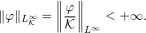 $$\begin{eqnarray}\Vert {\it\varphi}\Vert _{L_{{\mathcal{K}}}^{\infty }}=\biggl\|\frac{{\it\varphi}}{{\mathcal{K}}}\biggr\|_{L^{\infty }}<+\infty .\end{eqnarray}$$
Theorem 2.25 (exponential convergence in weighted $L^{\infty }$-spaces).

Suppose that Assumptions 2.23 and 2.24 hold. Then  $P$ admits a unique invariant probability measure
 ${\it\pi}$. This measure is such that
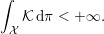 $$\begin{eqnarray}\int _{{\mathcal{X}}}{\mathcal{K}}\,\text{d}{\it\pi}<+\infty .\end{eqnarray}$$
Moreover, there exist  $C>0$ and
 $r\in (0,1)$ such that, for any
 ${\it\varphi}\in L_{{\mathcal{K}}}^{\infty }({\mathcal{X}})$ and any
 $n\in \mathbb{N}$,
 $$\begin{eqnarray}\biggl\|P^{n}{\it\varphi}-\int _{{\mathcal{X}}}{\it\varphi}\,\text{d}{\it\pi}\biggr\|_{L_{{\mathcal{K}}}^{\infty }}\leqslant Cr^{n}\biggl\|{\it\varphi}-\int _{{\mathcal{X}}}{\it\varphi}\,\text{d}{\it\pi}\biggr\|_{L_{{\mathcal{K}}}^{\infty }}.\end{eqnarray}$$
The proof of this result can be read in Hairer and Mattingly (Reference Hairer and Mattingly2011). Let us summarize the main steps. The
first idea is to introduce a family of distances  $d_{a}$ on
 ${\mathcal{X}}$ (with
 $a>0$), and to consider the induced Lipschitz seminorms
 $\Vert \cdot \Vert _{a}$ on real-valued functions defined on
 ${\mathcal{X}}$. These seminorms turn out to be equivalent to the
 $L_{{\mathcal{K}}}^{\infty }({\mathcal{X}})$-norm (up to the addition of constants to the functions under
consideration). Moreover, it is possible to prove a contraction principle of the
form
 $$\begin{eqnarray}|P{\it\varphi}(x)-P{\it\varphi}(y)|\leqslant rd_{a}(x,y)\Vert {\it\varphi}\Vert _{a}\end{eqnarray}$$
for some constant  $r\in (0,1)$, which implies a contraction principle for the operator
 $P$ considered on
 $L_{{\mathcal{K}}}^{\infty }({\mathcal{X}})$ endowed with the seminorm
 $\Vert \cdot \Vert _{a}$. The existence of the invariant measure is finally obtained by a
fixed-point theorem, and (2.65)
is deduced from the contraction inequality upon starting from
 $y$ distributed according to the invariant measure
 ${\it\pi}$. The prefactor
 $C\geqslant 1$ is related to the equivalence of the
 $\Vert \cdot \Vert _{L_{{\mathcal{K}}}^{\infty }}$ and
 $\Vert \cdot \Vert _{a}$ norms (as for the proof of hypocoercivity; see the comment after
Theorem 2.15).
The key point in the proof is therefore to obtain the contraction
inequality (2.66).
This is done by distinguishing the cases  ${\mathcal{K}}(x)+{\mathcal{K}}(y)\geqslant R$ (in this situation, the Lyapunov condition is used) or
 ${\mathcal{K}}(x)+{\mathcal{K}}(y)\leqslant R$ (the contraction then relies on the coupling ensured by the
minorization condition).
Let us now present a more compact reformulation of (2.65) in terms of operators. Introduce
 $$\begin{eqnarray}L_{{\mathcal{K}},0}^{\infty }({\mathcal{X}})=\biggl\{{\it\varphi}\in L_{{\mathcal{K}}}^{\infty }({\mathcal{X}})\,\bigg|\,\int _{{\mathcal{X}}}{\it\varphi}\,\text{d}{\it\pi}=0\biggr\}.\end{eqnarray}$$
Then (2.65) can
be equivalently written as an inequality for bounded operators on  $L_{{\mathcal{K}},0}^{\infty }({\mathcal{X}})$:
 $$\begin{eqnarray}\Vert P^{n}\Vert _{{\mathcal{B}}(L_{{\mathcal{K}},0}^{\infty })}\leqslant Cr^{n}.\end{eqnarray}$$
The exponential convergence allows us to obtain bounds on the resolvent  $\text{Id}-P$, which will prove useful in various contexts (for error
estimates on time discretizations or for the definition of the asymptotic variance
of Markov chains). The following result is the version of
Proposition 2.1
obtained in the context of this section.
Corollary 2.26 (invertibility of $\text{Id}-P$).

Let Assumptions 2.23 and 2.24 hold.
Then the bounded operator  $\text{Id}-P$ is invertible on
 $L_{{\mathcal{K}},0}^{\infty }({\mathcal{X}})$, and
 $$\begin{eqnarray}\Vert (\text{Id}-P)^{-1}\Vert _{{\mathcal{B}}(L_{{\mathcal{K}},0}^{\infty })}\leqslant \frac{C}{1-r}.\end{eqnarray}$$
Proof. Note that the sum  $\sum _{n\geqslant 0}P^{n}$ is convergent in
 ${\mathcal{B}}(L_{{\mathcal{K}},0}^{\infty })$ in view of (2.67). In addition, a simple computation gives
 $$\begin{eqnarray}(\text{Id}-P)\mathop{\sum }_{n=0}^{+\infty }P^{n}=\biggl(\mathop{\sum }_{n=0}^{+\infty }P^{n}\biggr)(\text{Id}-P)=\text{Id}.\end{eqnarray}$$
This shows that  $\text{Id}-P$ is invertible and
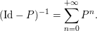 $$\begin{eqnarray}(\text{Id}-P)^{-1}=\mathop{\sum }_{n=0}^{+\infty }P^{n}.\end{eqnarray}$$
Moreover,
 $$\begin{eqnarray}\Vert (\text{Id}-P)^{-1}\Vert _{{\mathcal{B}}(L_{{\mathcal{K}},0}^{\infty })}\leqslant \mathop{\sum }_{n=0}^{+\infty }\Vert P^{n}\Vert _{{\mathcal{B}}(L_{{\mathcal{K}},0}^{\infty })}\leqslant C\mathop{\sum }_{n=0}^{+\infty }r^{n}=\frac{C}{1-r},\end{eqnarray}$$
which gives the claimed upper bound.
2.4.2 Application to Langevin and overdamped Langevin dynamics
To apply the convergence results to the stochastic evolutions typically
encountered in molecular dynamics, we fix some time  $t_{0}>0$ and consider the evolution operator
 $$\begin{eqnarray}P=\text{e}^{t_{0}{\mathcal{L}}},\end{eqnarray}$$
where  ${\mathcal{L}}$ is the generator of the dynamics under consideration. For
simplicity, we consider the dynamics (1.8) and (1.9), for which the force
 $-{\rm\nabla}V(q)$ is a gradient field. The results obtained below, however, can
easily be extended to more general force fields. This is one of the main interests
of weighted
 $L^{\infty }$ estimates: they do not require structural assumptions on the
type of dynamics considered.
We first discuss how to establish the Lyapunov condition (2.62) in Assumption 2.23 for Langevin and overdamped
Langevin dynamics. Let us start by recalling that, as discussed after
Assumption 2.23, it
is trivial to satisfy a Lyapunov condition when the state space is compact, by
choosing  ${\mathcal{K}}=\mathbf{1}$. This situation is encountered for overdamped Langevin dynamics
when
 ${\mathcal{D}}$ is compact. For overdamped Langevin dynamics in unbounded
position spaces, or Langevin dynamics (for which the momentum space is always
unbounded), the Lyapunov condition (2.62) can be established on the basis of a Lyapunov
condition stated in terms of the generator of the dynamics. Indeed, assume that
the following inequality is true for some
 $a>0$ and
 $b\geqslant 0$, and a given Lyapunov function
 ${\mathcal{K}}\geqslant 1$:
 $$\begin{eqnarray}{\mathcal{L}}{\mathcal{K}}\leqslant -a{\mathcal{K}}+b.\end{eqnarray}$$
This leads, by a time integration on the interval  $[0,s]$, to
 $$\begin{eqnarray}\text{e}^{s{\mathcal{L}}}{\mathcal{K}}\leqslant \text{e}^{-as}{\mathcal{K}}+\frac{b}{a}(1-\text{e}^{-as})\leqslant \text{e}^{-as}{\mathcal{K}}+\frac{b}{a}.\end{eqnarray}$$
In particular, for  $s=t_{0}$, we obtain
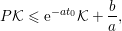 $$\begin{eqnarray}P{\mathcal{K}}\leqslant \text{e}^{-at_{0}}{\mathcal{K}}+\frac{b}{a},\end{eqnarray}$$
which is (2.62) with  ${\it\alpha}=\text{e}^{-at_{0}}\in (0,1)$ and
 $R=b/a\geqslant 0$. We therefore choose
 ${\mathcal{K}}$ in order for (2.69) to be satisfied. For overdamped Langevin dynamics in
unbounded spaces, a typical choice is
 ${\mathcal{K}}_{n}(q)=|q|^{n}$ for
 $n\geqslant 2$. In this case, for all
 $q\in {\mathcal{D}}$,
 $$\begin{eqnarray}{\mathcal{L}}{\mathcal{K}}_{n}(q)=n\biggl(-{\rm\nabla}V(q)\cdot q+\frac{d+n-2}{{\it\beta}}\biggr)|q|^{n-2}.\end{eqnarray}$$
Some assumptions on the asymptotic behaviour of the drift are needed at this stage, such as
 $$\begin{eqnarray}q\cdot {\rm\nabla}V(q)\geqslant A|q|^{2}-B,\quad \text{for all }q\in {\mathcal{D}},\end{eqnarray}$$
for some constant  $A>0$ and
 $B\in \mathbb{R}$. This condition is satisfied for potentials
 $V(q)$ behaving at infinity as
 $|q|^{k}$ with
 $k\geqslant 2$. With (2.72),
the Lyapunov condition (2.69)
indeed holds since, for all
 $q\in {\mathcal{D}}$,
 $$\begin{eqnarray}{\mathcal{L}}{\mathcal{K}}_{n}(q)\leqslant -An{\mathcal{K}}_{n}(q)+\frac{n(d+n-2)}{{\it\beta}}|q|^{n-2}+Bn,\end{eqnarray}$$
so that
 $$\begin{eqnarray}\limsup _{|q|\rightarrow +\infty }\,\frac{{\mathcal{L}}{\mathcal{K}}_{n}(q)}{{\mathcal{K}}_{n}(q)}\leqslant -An.\end{eqnarray}$$
There exist therefore  $b_{n}\geqslant 0$ such that
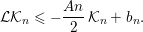 $$\begin{eqnarray}{\mathcal{L}}{\mathcal{K}}_{n}\leqslant -\frac{An}{2}\,{\mathcal{K}}_{n}+b_{n}.\end{eqnarray}$$
For Langevin dynamics, the choice  ${\mathcal{K}}_{n}(q,p)=1+|p|^{n}$ with
 $n\geqslant 2$ is appropriate when the position space is compact. Indeed, with
 $m_{+}$ defined in (2.46), for all
 $(q,p)\in {\mathcal{E}}$,
 $$\begin{eqnarray}\displaystyle {\mathcal{L}}{\mathcal{K}}_{n}(q,p) & = & \displaystyle -np^{T}{\rm\nabla}V(q)|p|^{n-2}-{\it\gamma}n\biggl(p^{T}M^{-1}p-\frac{n+d-2}{{\it\beta}}\biggr)|p|^{n-2}\nonumber\\ \displaystyle & {\leqslant} & \displaystyle -\frac{{\it\gamma}n}{m_{+}}|p|^{n}+n\Vert {\rm\nabla}V\Vert _{L^{\infty }}|p|^{n-1}+\frac{{\it\gamma}n(n+d-2)}{{\it\beta}}|p|^{n-2},\nonumber\end{eqnarray}$$
so that there exists  $b_{n}\geqslant 0$ such that
 $$\begin{eqnarray}{\mathcal{L}}{\mathcal{K}}_{n}\leqslant -\frac{{\it\gamma}n}{2m_{+}}\,{\mathcal{K}}_{n}+b_{n}.\end{eqnarray}$$
For Langevin dynamics in an unbounded position space  ${\mathcal{D}}$, a possible choice is (see Mattingly, Stuart and Higham Reference Mattingly, Stuart and Higham2002)
 $$\begin{eqnarray}{\mathcal{K}}_{n}(q,p)=\biggl(1+H(q,p)-V_{-}+\frac{{\it\gamma}}{2}p^{T}M^{-1}q+\frac{{\it\gamma}^{2}}{4}q^{T}M^{-1}q\biggr)^{n},~~\text{for all }(q,p)\in {\mathcal{E}},\end{eqnarray}$$
where we assume that the potential energy function  $V(q)$ is bounded from below by
 $V_{-}>-\infty$ and that there exist
 $A,B>0$ and
 $C\in \mathbb{R}$ such that
 $$\begin{eqnarray}q^{T}M^{-1}{\rm\nabla}V(q)\geqslant AV(q)+Bq^{T}M^{-1}q+C,\quad \text{for all }q\in {\mathcal{D}}.\end{eqnarray}$$
This condition is satisfied for instance when  $V(q)$ behaves at infinity as
 $|q|^{k}$ with
 $k\geqslant 2$. Then, for any
 $n\geqslant 1$, we have
 ${\mathcal{K}}_{n}(q,p)\geqslant 1$ and
 ${\mathcal{K}}_{n}(q,p)\rightarrow +\infty$ as
 $|(q,p)|\rightarrow +\infty$. In addition, there exist
 $a>0$ and
 $b_{n}\in \mathbb{R}$ such that
 $$\begin{eqnarray}{\mathcal{L}}{\mathcal{K}}_{n}\leqslant -na{\mathcal{K}}_{n}+b_{n}.\end{eqnarray}$$
Note that the Lyapunov function has a component  $p^{T}M^{-1}q$ which allows us to retrieve some dissipation in the
 $q$-direction from the dissipation in the momenta. This feature is
reminiscent of the cross-derivative used in the scalar product introduced for the
proof of hypocoercivity in Section 2.3 (see the terms proportional to
 $b$ in (2.38)).
Let us now discuss how to obtain the minorization condition in
Assumption 2.24. Note
first that this condition can be rewritten as: for any Borel set  $S\subset {\mathcal{X}}$,
 $$\begin{eqnarray}P(x,S)\geqslant {\it\eta}{\it\lambda}(S).\end{eqnarray}$$
A convenient way to obtain such a lower bound is to first establish that the transition kernel can be rewritten as
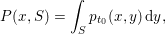 $$\begin{eqnarray}P(x,S)=\int _{S}p_{t_{0}}(x,y)\,\text{d}y,\end{eqnarray}$$
where the density  $p_{t_{0}}(x,y)$ of the transition kernel is a
 $C^{\infty }$ function of
 $(x,y)\in {\mathcal{X}}^{2}$. This is the case, appealing to parabolic regularity for
overdamped Langevin dynamics and hypoellipticity for Langevin dynamics (see for
instance the discussion in Section 8 of Rey-Bellet Reference Rey-Bellet, Attal, Joye and Pillet2006). The second step is to prove that, for
any open set
 ${\mathcal{O}}\subset {\mathcal{X}}$ and any
 $x\in {\mathcal{X}}$, we have
 $$\begin{eqnarray}P(x,{\mathcal{O}})>0.\end{eqnarray}$$
This is proved by controllability arguments, as reviewed in
Section 7 of Rey-Bellet (Reference Rey-Bellet, Attal, Joye and Pillet2006),
where the cases of Langevin and overdamped Langevin are explicitly treated; see
also Mattingly, Stuart and Higham (Reference Mattingly, Stuart and Higham2002) and Talay (Reference Talay2002) for
Langevin dynamics. The idea is to choose some end configuration  $y\in {\mathcal{O}}$, and to construct a realization of the Brownian motion such that
the dynamics started at
 $x$ ends up at
 $y$ at time
 $t_{0}$. The continuity of the solutions of SDEs with respect to the
realization of the Brownian motion then leads to (2.76). In view of (2.75), the condition (2.76) in fact shows that, for any
compact set
 ${\mathcal{C}}\subset {\mathcal{X}}$,
 $$\begin{eqnarray}p_{t_{0}}(x,y)>0,\quad \text{for all }(x,y)\in {\mathcal{C}}^{2}.\end{eqnarray}$$
Since  $(x,y)\mapsto p_{t_{0}}(x,y)$ is continuous, this proves the existence of
 ${\it\delta}_{{\mathcal{C}}}>0$ such that
 $p_{t_{0}}(x,y)\geqslant {\it\delta}_{{\mathcal{C}}}$ for all
 $(x,y)\in {\mathcal{C}}^{2}$. The minorization condition then follows by considering the
probability measure
 $$\begin{eqnarray}{\it\lambda}(\text{d}y)=\frac{1}{|{\mathcal{C}}|}\mathbf{1}_{{\mathcal{C}}}(y)\,\text{d}y,\end{eqnarray}$$
and setting  ${\it\eta}={\it\delta}_{{\mathcal{C}}}|{\mathcal{C}}|$.
At this stage, we have discussed how to obtain Assumptions 2.23 and 2.24. This already implies the decay
estimates (2.65) by
Theorem 2.25. These
bounds correspond to evolutions observed at integer multiples of the reference time  $t_{0}$. Let us now finally show how to deduce an exponential
convergence result at all times
 $t\geqslant 0$. To this end, we decompose the time
 $t$ as
 $t=kt_{0}+{\it\theta}$ with
 $k\in \mathbb{N}$ and
 ${\it\theta}\in [0,t_{0})$. Then, for any
 ${\it\varphi}\in L_{{\mathcal{K}},0}^{\infty }({\mathcal{X}})$ we obtain
 $$\begin{eqnarray}\Vert \text{e}^{t{\mathcal{L}}}{\it\varphi}\Vert _{L_{{\mathcal{K}}}^{\infty }}\leqslant Cr^{k}\Vert \text{e}^{{\it\theta}{\mathcal{L}}}{\it\varphi}\Vert _{L_{{\mathcal{K}}}^{\infty }}\leqslant Cr^{k}\sup _{0\leqslant s\leqslant t_{0}}\Vert \text{e}^{s{\mathcal{L}}}{\it\varphi}\Vert _{L_{{\mathcal{K}}}^{\infty }}.\end{eqnarray}$$
Now, the inequality
 $$\begin{eqnarray}|{\it\varphi}(x)|\leqslant \Vert {\it\varphi}\Vert _{L_{{\mathcal{K}}}^{\infty }}{\mathcal{K}}(x),\quad \text{for all }x\in {\mathcal{X}},\end{eqnarray}$$
leads to
 $$\begin{eqnarray}\Vert \text{e}^{s{\mathcal{L}}}{\it\varphi}\Vert _{L_{{\mathcal{K}}}^{\infty }}\leqslant \Vert {\it\varphi}\Vert _{L_{{\mathcal{K}}}^{\infty }}\biggl\|\frac{\text{e}^{s{\mathcal{L}}}{\mathcal{K}}}{{\mathcal{K}}}\biggr\|_{L^{\infty }}.\end{eqnarray}$$
In view of the inequality (2.70), for any  $s\geqslant 0$ we obtain
 $$\begin{eqnarray}\biggl\|\frac{\text{e}^{s{\mathcal{L}}}{\mathcal{K}}}{{\mathcal{K}}}\biggr\|_{L^{\infty }}\leqslant \text{e}^{-as}+\frac{b}{a}\biggl\|\frac{1}{{\mathcal{K}}}\biggr\|_{L^{\infty }}\leqslant 1+\frac{b}{a}.\end{eqnarray}$$
Upon introducing  ${\it\kappa}=-\log (r)/t_{0}>0$, (2.77) implies
 $$\begin{eqnarray}\Vert \text{e}^{t{\mathcal{L}}}{\it\varphi}\Vert _{L_{{\mathcal{K}}}^{\infty }}\leqslant C\biggl(1+\frac{b}{a}\biggr)\text{e}^{-{\it\kappa}kt_{0}}\Vert {\it\varphi}\Vert _{L_{{\mathcal{K}}}^{\infty }}\leqslant \widetilde{C}\text{e}^{-{\it\kappa}t}\Vert {\it\varphi}\Vert _{L_{{\mathcal{K}}}^{\infty }},\end{eqnarray}$$
with
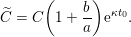 $$\begin{eqnarray}\widetilde{C}=C\biggl(1+\frac{b}{a}\biggr)\text{e}^{{\it\kappa}t_{0}}.\end{eqnarray}$$
The exponential convergence result (2.78) leads to the following bounds on the resolvent.
Corollary 2.27. Consider one of the following situations:
(1) For overdamped Langevin dynamics, set
${\mathcal{X}}={\mathcal{D}}$ and ${\it\pi}={\it\nu}$, and assume either that the position space is
compact, in which case ${\mathcal{K}}=\mathbf{1}$, or that (2.72) holds, in which case ${\mathcal{K}}(q)=1+|q|^{n}$ for some $n\geqslant 2$.(2) For Langevin dynamics, set
${\mathcal{X}}={\mathcal{E}}$ and ${\it\pi}={\it\mu}$, and assume either that the position space is
compact, in which case ${\mathcal{K}}(q,p)=1+|p|^{n}$ for some $n\geqslant 2$, or that (2.74) holds, in which case ${\mathcal{K}}$ is given by (2.73) for some $n\geqslant 1$.








Then the operator  ${\mathcal{L}}$ is invertible on
 $L_{{\mathcal{K}},0}^{\infty }({\mathcal{X}})$, and the following equality holds in
 ${\mathcal{B}}(L_{{\mathcal{K}},0}^{\infty })$:
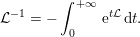 $$\begin{eqnarray}{\mathcal{L}}^{-1}=-\int _{0}^{+\infty }\,\text{e}^{t{\mathcal{L}}}\,\text{d}t.\end{eqnarray}$$
Moreover,
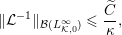 $$\begin{eqnarray}\Vert {\mathcal{L}}^{-1}\Vert _{{\mathcal{B}}(L_{{\mathcal{K}},0}^{\infty })}\leqslant \frac{\widetilde{C}}{{\it\kappa}},\end{eqnarray}$$
where  $\widetilde{C}$ and
 ${\it\kappa}$ are the same constants as in (2.78).
Although it is possible to keep track of the values of the various constants until
(2.78), the final rate of
convergence in weighted  $L^{\infty }$-spaces is often not very sharp. Generally, the difficulty is in
controlling the constant
 ${\it\eta}$ in the minorization condition of Assumption 2.24.
Remark 2.28 (sub-exponential convergence rates).
It is possible to weaken the Lyapunov condition (2.69) for instance as  ${\mathcal{L}}{\mathcal{K}}\leqslant -{\it\phi}({\mathcal{K}})+b$, where
 ${\it\phi}$ is a non-negative, non-decreasing, concave function such
that
 ${\it\phi}(x)/x\rightarrow 0$ as
 $x\rightarrow +\infty$. In this case, algebraic rates of decay are typically
obtained instead of exponential ones; see Douc, Fort and Guillin (Reference Douc, Fort and Guillin2009) or Cattiaux (Reference Cattiaux2014) for further details.
2.5 Spectral approaches
One interest of the approaches mentioned in the previous sections is that they can also be used for dynamics other than Langevin or overdamped Langevin dynamics. This is illustrated in Section 4, for example, where entropy techniques and logarithmic Sobolev inequalities play a crucial role in analysing non-linear partial parabolic equations related to adaptive importance sampling methods, and in Section 5, where Lyapunov techniques are useful for the study of non-reversible perturbations of Langevin or overdamped Langevin dynamics. However, when discussing the long-time behaviour of linear parabolic partial differential equations and the link with metastable stochastic processes, we could not avoid mentioning spectral approaches and semi-classical analysis.
Let us consider the overdamped Langevin process. Recall the definitions of the
infinitesimal generator  ${\mathcal{L}}$ (see (1.13)) and
its adjoint
 ${\mathcal{L}}^{\dagger }$:
 $$\begin{eqnarray}{\mathcal{L}}=-{\rm\nabla}V\cdot {\rm\nabla}+{\it\beta}^{-1}{\rm\Delta},\end{eqnarray}$$
which is symmetric on the Hilbert space  $L^{2}({\it\nu})$, and
 $$\begin{eqnarray}{\mathcal{L}}^{\dagger }=\text{div}({\rm\nabla}V.)+{\it\beta}^{-1}{\rm\Delta},\end{eqnarray}$$
which is symmetric on the Hilbert space  $L^{2}(1/{\it\nu})$. As explained in Section 2.2, the exponential convergence to equilibrium of the Kolmogorov forward
dynamics
 $$\begin{eqnarray}\partial _{t}{\it\psi}={\mathcal{L}}^{\dagger }{\it\psi}\end{eqnarray}$$
in the weighted  $L^{2}(1/{\it\nu})$-space is related to the fact that
 ${\it\nu}$ satisfies a Poincaré inequality (2.17). The two following assertions are
indeed equivalent by Proposition 2.3 and the fact that
 ${\it\psi}$ satisfies (2.80) if and only if
 $\partial _{t}({\it\psi}/{\it\nu})={\mathcal{L}}({\it\psi}/{\it\nu})$:
∙ For all
${\it\psi}_{0}$ such that ${\it\psi}_{0}/{\it\nu}\in L^{2}({\it\nu})$, and for all $t\geqslant 0$, where$$\begin{eqnarray}\biggl\|\frac{{\it\psi}(t,\cdot )}{{\it\nu}}-1\biggr\|_{L^{2}({\it\nu})}^{2}\leqslant \biggl\|\frac{{\it\psi}_{0}}{{\it\nu}}-1\biggr\|_{L^{2}({\it\nu})}^{2}\exp \biggl(-\frac{4Rt}{{\it\beta}}\biggr),\end{eqnarray}$$${\it\psi}$ satisfies (2.80) with initial condition ${\it\psi}(0,\cdot )={\it\psi}_{0}$, and $R>0$ is some constant.∙ The measure
${\it\nu}$ satisfies the following Poincaré inequality: $\text{for all }{\it\varphi}\in H^{1}({\it\nu})$, $$\begin{eqnarray}\int _{{\mathcal{D}}}\biggl({\it\varphi}-\int _{{\mathcal{D}}}{\it\varphi}\,\text{d}{\it\nu}\biggr)^{2}\,\text{d}{\it\nu}\leqslant \frac{1}{2R}\int _{{\mathcal{D}}}|{\rm\nabla}{\it\varphi}|^{2}\,\text{d}{\it\nu}.\end{eqnarray}$$




By noting that
 $$\begin{eqnarray}\int _{{\mathcal{D}}}|{\rm\nabla}{\it\varphi}|^{2}\,\text{d}{\it\nu}=-{\it\beta}\int _{{\mathcal{D}}}{\it\varphi}\,({\mathcal{L}}{\it\varphi})\,\text{d}{\it\nu},\end{eqnarray}$$
we observe that the optimal constant  $R$ is related to the first non-zero eigenvalue of the operator
 $-{\mathcal{L}}$ on
 $L^{2}({\it\nu})$:
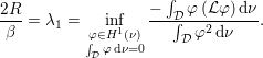 $$\begin{eqnarray}\frac{2R}{{\it\beta}}={\it\lambda}_{1}=\inf _{\substack{ {\it\varphi}\in H^{1}({\it\nu}) \\ \int _{{\mathcal{D}}}{\it\varphi}\,\text{d}{\it\nu}=0}}\frac{-\int _{{\mathcal{D}}}{\it\varphi}\,({\mathcal{L}}{\it\varphi})\,\text{d}{\it\nu}}{\int _{{\mathcal{D}}}{\it\varphi}^{2}\,\text{d}{\it\nu}}.\end{eqnarray}$$
Recall that the first eigenvalue of  ${\mathcal{L}}$ on
 $L^{2}({\it\nu})$ is
 ${\it\lambda}_{0}=0$, with associated eigenfunctions proportional to the constant
function
 $\mathbf{1}$. The corresponding eigenspace is non-degenerate since
 ${\mathcal{L}}{\it\varphi}=0$ implies that
 ${\it\varphi}$ is constant by (2.81). Therefore, the second eigenvalue
 ${\it\lambda}_{1}$ obtained by the Rayleigh–Ritz principle (2.82) is indeed the first non-zero
eigenvalue of
 $-{\mathcal{L}}$. The difference
 ${\it\lambda}_{1}-{\it\lambda}_{0}={\it\lambda}_{1}$ is called the spectral gap of the operator. The above discussion
already shows the importance of the spectrum of the operator
 ${\mathcal{L}}$ in understanding the long-time behaviour of (2.80).
In fact, in order to understand and quantify the metastability of overdamped Langevin
dynamics, it is interesting to consider not only the first eigenvalue of  ${\mathcal{L}}$ but an ensemble of small eigenvalues. In order to explain this, we
need to introduce the notion of the Witten Laplacian. The Witten Laplacian is an
operator which is unitarily equivalent to
 ${\mathcal{L}}$ and
 ${\mathcal{L}}^{\dagger }$, and which acts on the non-weighted (flat)
 $L^{2}$-space. Let us first recall that the spectrum of
 ${\mathcal{L}}$ is the same as the spectrum of
 ${\mathcal{L}}^{\dagger }$ in view of the unitary equivalence
 $$\begin{eqnarray}{\mathcal{L}}^{\dagger }=U{\mathcal{L}}U^{-1},\end{eqnarray}$$
where  $U$ is the unitary transformation defined by
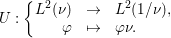 $$\begin{eqnarray}U:\left\{\begin{array}{@{}rcl@{}}L^{2}({\it\nu}) & \rightarrow & L^{2}(1/{\it\nu}),\\ {\it\varphi} & \mapsto & {\it\varphi}{\it\nu}.\end{array}\right.\end{eqnarray}$$
Now, the spectrum of these operators is also related to the spectrum
of a Witten Laplacian. For a function  $f:\mathbb{R}^{d}\rightarrow \mathbb{R}$ and a positive parameter
 $h$, the Witten LaplacianFootnote 8 is defined by
 $$\begin{eqnarray}{\rm\Delta}_{f,h}=(-h{\rm\nabla}+{\rm\nabla}f)\cdot (h{\rm\nabla}+{\rm\nabla}f)=-h^{2}{\rm\Delta}+(|{\rm\nabla}f|^{2}-h{\rm\Delta}f),\end{eqnarray}$$
considered on the flat Hilbert space  $L^{2}$. Note that this operator is of Schrödinger type, which
is convenient since the spectral properties of these operators are quite well
understood; see Reed and Simon (Reference Reed and Simon1975b). The spectrum of
 ${\mathcal{L}}$ is
 $-{\it\beta}$ times the spectrum of
 ${\rm\Delta}_{V/2,{\it\beta}^{-1}}$ since
 ${\mathcal{L}}$ and
 $-{\it\beta}{\rm\Delta}_{V/2,{\it\beta}^{-1}}$ are unitarily equivalent (see (2.14)), that is,
 $$\begin{eqnarray}-{\it\beta}{\rm\Delta}_{V/2,{\it\beta}^{-1}}=\widetilde{U}{\mathcal{L}}\widetilde{U}^{-1},\end{eqnarray}$$
where  $\widetilde{U}$ is the unitary transformation
 $$\begin{eqnarray}\widetilde{U}:\left\{\begin{array}{@{}rcl@{}}L^{2}({\it\nu}) & \rightarrow & L^{2},\\ {\it\varphi} & \mapsto & {\it\varphi}\sqrt{{\it\nu}}.\end{array}\right.\end{eqnarray}$$
Many outstanding mathematicians have contributed to the analysis of
the small eigenvalues of Witten Laplacians, and the associated eigenvectors, in the
so-called semi-classical limit, namely when  $h\rightarrow 0$. In our context this corresponds to the low-temperature regime
 ${\it\beta}^{-1}\rightarrow 0$. We refer the reader to Witten (Reference Witten1982), Helffer and Sjöstrand (Reference Helffer and Sjöstrand1985), Cycon, Froese, Kirsch and Simon (Reference Cycon, Froese, Kirsch and Simon1987), Burghelea (Reference Burghelea1997) and Zhang
(Reference Zhang2001) for an introduction to the
semi-classical analysis of Witten Laplacians and its famous application to Morse
inequalities. It is not our aim here to present the details of this theory. Let us
simply mention the main results that are of interest in the context of understanding
the metastability of overdamped Langevin dynamics. We assume that the potential
 $V:\mathbb{R}^{d}\rightarrow \mathbb{R}$ is a Morse function (i.e., its critical points are
non-degenerate) and that
 $$\begin{eqnarray}\lim _{|x|\rightarrow \infty }\frac{|{\rm\nabla}V|^{2}}{2}-{\it\beta}^{-1}{\rm\Delta}V=+\infty\end{eqnarray}$$
for sufficiently small  ${\it\beta}^{-1}\ ($so the spectrum of
 ${\rm\Delta}_{V/2,{\it\beta}^{-1}}$ is discrete. Then, we have the following asymptotic results, in the
limit
 ${\it\beta}\rightarrow \infty$ (see Helffer, Klein and Nier Reference Helffer, Klein and Nier2004).
∙ The operator
${\rm\Delta}_{V/2,{\it\beta}^{-1}}$ admits exactly $m_{0}$ eigenvalues (including $0$) which are smaller than $\exp (-c{\it\beta})$ for a constant $c>0$. All the other eigenvalues are bounded from below by a
constant. The integer $m_{0}$ is the number of local minima of $V$.∙ The associated eigenfunctions are of the form
${\it\chi}_{i}\exp (-{\it\beta}V/2)$, where the functions ${\it\chi}_{i}$ are locally constant over the basins of attraction of the
local minima of $V$ for the gradient dynamics ${\dot{x}}=-{\rm\nabla}V(x)$.∙ The smallest eigenvalue is
${\it\lambda}_{0}=0$, associated with the eigenvector $\exp (-{\it\beta}V/2)$. The other positive small eigenvalues ${\it\lambda}_{1}<{\it\lambda}_{2}<\cdots <{\it\lambda}_{m_{0}-1}$ satisfy the Eyring–Kramers law: for $i=1,\ldots ,m_{0}-1$, (2.83)where$$\begin{eqnarray}\displaystyle {\it\lambda}_{i}=\frac{|\hat{{\it\lambda}}(s_{j(i)})|}{2{\it\beta}{\it\pi}}\sqrt{\frac{\det ({\rm\nabla}^{2}V(x_{i}))}{|\det ({\rm\nabla}^{2}V(s_{j(i)}))|}}\,\text{e}^{-{\it\beta}[V(s_{j(i)})-V(x_{i})]}(1+\text{O}({\it\beta}^{-1})), & & \displaystyle\end{eqnarray}$$$\{x_{0},x_{1},\ldots ,x_{m_{0}-1}\}$ is the set of local minima of $V$ and, for $i\in \{1,\ldots ,m_{0}-1\}$, $s_{j(i)}$ is a saddle point attached to the local minimum $x_{i}$, $\hat{{\it\lambda}}(s_{j(i)})$ being the negative eigenvalue of ${\rm\nabla}^{2}V(s_{j(i)})$. Let us now explain how a saddle point $s_{j(i)}$ is attached to each local minimum $x_{i}$. From a local minimum $x_{i}$, one considers the communication height between $x_{i}$ and the union of small balls around local minima which are
lower in energy than $V(x_{i})$, denoted by $B_{i}$: where$$\begin{eqnarray}H(x_{i},B_{i})=\inf _{{\it\gamma}\in {\mathcal{P}}(x_{i},B_{i})}\sup _{t\in [0,1]}V({\it\gamma}(t))-V(x_{i}),\end{eqnarray}$$${\mathcal{P}}(x_{i},B_{i})$ denotes the set of continuous paths from $[0,1]$ to ${\mathcal{D}}$ such that ${\it\gamma}(0)=x_{i}$ and ${\it\gamma}(1)\in B_{i}$. For each $i\in \{1,\ldots ,m_{0}-1\}$, the communication height $H(x_{i},B_{i})$ is generally reached at a unique order-one saddle point $s_{j(i)}$: Note that we implicitly assume here that$$\begin{eqnarray}H(x_{i},B_{i})=V(s_{j(i)})-V(x_{i}).\end{eqnarray}$$$x_{0}$ is the global minimum and the other local minima $(x_{i})_{1\leqslant i\leqslant m_{0}-1}$ are ordered such that in order to ensure that$$\begin{eqnarray}H(x_{1},B_{1})>\cdots >H(x_{m_{0}-1},B_{m_{0}-1}),\end{eqnarray}$$${\it\lambda}_{1}<{\it\lambda}_{2}<\cdots <{\it\lambda}_{m_{0}}$.














One ingredient for the proof of the results provided in Helffer, Klein and
Nier (Reference Helffer, Klein and Nier2004) is to introduce the
Witten Laplacian on 1-forms, which can be identified with the following operator on
vector fields: for  $w:{\mathcal{D}}\mapsto \mathbb{R}^{d}$,
 $$\begin{eqnarray}({\rm\Delta}_{f,h}^{(1)}w)_{i}=-h^{2}{\rm\Delta}w_{i}+(|{\rm\nabla}f|^{2}-h{\rm\Delta}f)w_{i}+2h(({\rm\nabla}^{2}f)w)_{i}.\end{eqnarray}$$
Note that if  $u:{\mathcal{D}}\rightarrow \mathbb{R}$ is an eigenvector for
 ${\rm\Delta}_{f,h}$, then
 $h{\rm\nabla}u+u{\rm\nabla}f$ is either 0 or an eigenvector for
 ${\rm\Delta}_{f,h}^{(1)}$. Then one can see that the eigenvalues of
 ${\rm\Delta}_{f,h}$ are the square of the singular values of the operator
 $d_{f,h}=h{\rm\nabla}+{\rm\nabla}f$ which maps
 $0$-forms to
 $1$-forms, since
 ${\rm\Delta}_{f,h}=d_{f,h}^{\ast }d_{f,h}$ (where
 $d_{f,h}^{\ast }=-h\,\text{div}+{\rm\nabla}f$ is the
 $L^{2}$-adjoint of
 $d_{f,h}$). Using a basis of quasi-modes associated with the small
eigenvalues of
 ${\rm\Delta}_{f,h}$ and
 ${\rm\Delta}_{f,h}^{(1)}$, one is then able to analyse the singular values of
 $d_{f,h}$ restricted to the finite-dimensional subspaces spanned by these
quasi-modes. The quasi-modes are built using the following important fact: the
eigenvectors of
 ${\rm\Delta}_{f,h}$ (resp. of
 ${\rm\Delta}_{f,h}^{(1)}$) are concentrated around the local minima (resp. the
order-one saddle points) of the function
 $f$. This can be proved using so-called semi-classical Agmon estimates
(Simon Reference Simon1984, Helffer and Sjöstrand
Reference Helffer and Sjöstrand1984). For generalizations to manifolds
with boundaries and to Witten Laplacians on
 $p$-forms, we refer to Helffer and Nier (Reference Helffer and Nier2006) and Le Peutrec, Nier and Viterbo (Reference Le Peutrec, Nier and Viterbo2013).
Bovier et al. (Reference Bovier, Eckhoff, Gayrard and Klein2004a, Reference Bovier, Gayrard and Klein2004b) developed another analytic approach to proving
(2.83). In particular, they
proved that, for  $i\in \{1,\ldots ,m_{0}-1\}$,
 $$\begin{eqnarray}{\it\lambda}_{i}^{-1}=\mathbb{E}_{x_{i}}({\it\tau}_{B_{i}})(1+\text{O}(\text{e}^{-{\it\beta}c}))\end{eqnarray}$$
for some positive constant  $c>0$, where
 $\mathbb{E}_{x_{i}}({\it\tau}_{B_{i}})$ denotes the mean time to reach
 $B_{i}$ starting from
 $x_{i}$.
We would like to emphasize that we do not provide these results with all the required assumptions (in particular, it is assumed that the communication heights are all different, and that the communication height is attained at a unique saddle point). For more details of this subject, we refer for example to the lecture notes by Helffer and Nier (Reference Helffer and Nier2005), and also to the nice review by Berglund (Reference Berglund2013).
From a modelling viewpoint, this spectral approach gives the cascade of relevant time
scales to reach from a local minimum  $x_{i}$ (for
 $i\in \{1,\ldots ,m_{0}-1\}$) any other local minimum which is lower in energy (and in
particular the global minimum
 $x_{0}$). This does not provide us with any information about the typical
time scale to go from any local minimum to any other local minimum (for example from
the global minimum to the second lower minimum). We will come back to this in
Sections 6.3
and 6.4, where we use a spectral
approach on bounded domains (rather than on the full state space
 ${\mathcal{D}}$) to derive a Markov state model; see also the article by
Lelièvre and Nier Reference Lelièvre and Nier2015. We also
refer to the works by Maier and Stein (Reference Maier and Stein1993,
Reference Maier and Stein1997), Naeh, Klosek, Matkowsky and Schuss
(Reference Naeh, Klosek, Matkowsky and Schuss1990) and Matkowsky and Schuss (Reference Matkowsky and Schuss1979) for other approaches to this problem using
formal expansions of singularly perturbed partial differential equations. An
interesting work relating spectral gaps for the infinitesimal generator restricted to
metastable states with the global spectral gap is that of Menz and Schlichting (Reference Menz and Schlichting2014). Notice also that spectral approaches are
very relevant to energetic barriers but not to entropic barriers (for which the Morse
assumption may typically be wrong: see Figure 1.1(c, d)).
For numerical purposes, these results are interesting for the following reason. As
explained above, the existence of small eigenvalues can be related to the existence
of metastable states, characterized as the regions where the eigenfunctions of  ${\mathcal{L}}$ are constant. This can be used to identify the metastable states.
More importantly, if one wants to define an optimal Galerkin projection of the
operator
 ${\mathcal{L}}$ onto a discrete space, it is natural to introduce the Galerkin
basis consisting of the eigenvectors associated with the smallest eigenvalues. This
indeed leads to the smallest errors (in the
 $L^{2}({\it\nu})$-norm) for the semi-group
 $\text{e}^{t{\mathcal{L}}}$. By using the Galerkin projection, one can thus build from the
original dynamics an approximated Markov dynamics in a discrete state space (a
so-called Markov state model, or kinetic Monte Carlo model: see Bowman,
Pande and Noé Reference Bowman, Pande and Noé2014). This has been
extensively investigated by C. Schütte and his collaborators,
starting with the seminal work of Schütte (Reference Schütte1998). In fact, Schütte
et al. look at the eigenvalues close to
 $1$ for the so-called transfer operator
 $P_{t}=\text{e}^{t{\mathcal{L}}}$ (for a well-chosen lag time
 $t>0$), which is equivalent to looking at the small positive eigenvalues
of
 $-{\mathcal{L}}$. In practice, the eigenfunctions can be approximated using the
committor functions associated with core sets (i.e., disjoint
subsets of the configuration space
 ${\mathcal{D}}$). For more details of this approach, we refer to the recent book by
Sarich and Schütte (Reference Sarich and Schütte2013). We will
come back to the relation between original Langevin or overdamped Langevin dynamics
with a discrete state-space Markov process in Section 6.3 below, where another projection technique will be presented
using the notion of quasi-stationary distributions.
For Langevin dynamics, similar questions can be raised. For example, the Eyring–Kramers law (2.83) can be generalized to Langevin dynamics: see Maier and Stein (Reference Maier and Stein1993, Reference Maier and Stein1997), Naeh et al. (Reference Naeh, Klosek, Matkowsky and Schuss1990), Matkowsky and Schuss (Reference Matkowsky and Schuss1979), Hérau, Hitrik and Sjöstrand (Reference Hérau, Hitrik and Sjöstrand2011) or Bouchet and Reygner (Reference Bouchet and Reygner2015). In general, the eigenvectors cannot be written in a separated form in terms of positions and momenta. Metastable states should therefore be defined both in terms of positions and velocities. This raises some difficulties from modelling and numerical viewpoints. We refer to Sarich and Schütte (Reference Sarich and Schütte2013) for discussions on this aspect.
Remark 2.29. In this section we have discussed the spectral properties of  ${\mathcal{L}}$ in the weighted
 $L^{2}({\it\nu})$-space since this is a very natural functional space for
overdamped Langevin dynamics, in particular in terms of self-adjointness. There
are also interesting results concerning the spectrum in the weighted space
 $L_{{\mathcal{K}}}^{\infty }$, where
 ${\mathcal{K}}$ is a Lyapunov function, as introduced in
Section 2.4. We refer for
example to Sarich and Schütte (Reference Sarich and Schütte2013, Section 4.3.1) for a discussion and references on this
question. See also Cattiaux, Guillin and Zitt (Reference Cattiaux, Guillin and Zitt2013) for related questions on the link between Lyapunov conditions
and spectral gaps, and Cattiaux, Guillin and Wu (Reference Cattiaux, Guillin and Wu2009) for the link between Lyapunov
conditions and logarithmic Sobolev inequalities.
3 Computing thermodynamic averages
In this section we discuss the errors in the practical estimation of canonical averages.
As already mentioned in Section 1 (see
in particular the discussion after (1.5)), the challenging part is to sample the canonical measure  ${\it\nu}(\text{d}q)=Z_{{\it\nu}}^{-1}\,\text{e}^{-{\it\beta}V(q)}\,\text{d}q$ on the position space
 ${\mathcal{D}}$. Without restriction of generality, we can therefore restrict
ourselves to observables depending only on
 $q$. The typical way to estimate canonical averages
 $\int _{{\mathcal{D}}}{\it\varphi}\,\text{d}{\it\nu}$ is to first discretize in time a dynamics ergodic with respect to
 ${\it\nu}$ (such as the Langevin (1.9) or overdamped Langevin (1.8) dynamics), and then to compute averages along one realization of this
dynamics. The long-time convergence of such an estimator requires the discretized
dynamics to be ergodic as well, although the corresponding ergodic measure generally
differs from
 ${\it\nu}$ because of the time discretization.
In practice, choosing a good initial condition  $q_{0}$ (namely such that
 $V(q_{0})$ is not too large) may be difficult. This is why a burn-in phase is
usually performed, during which the sampled configurations are discarded. Actual
averages start after this initial relaxation. We will not discuss this practical aspect
further.
Note also that it is possible to run several realizations of the discretized dynamics in parallel, which provides faster results in terms of wall clock time. Some care has to be taken in order to ensure that the initial conditions, and thus the realizations, are indeed independent (for instance by performing independent burn-in phases for each realizations). This computational overhead sometimes motivates practitioners to estimate average properties with a single, long trajectory.
To perform the numerical analysis allowing us to quantify errors made in the trajectorial averages of discretized dynamics, we first review results ensuring the ergodicity of continuous dynamics in Section 3.1. We next turn to the discretization of continuous dynamics and the ergodic properties of the resulting numerical schemes in Section 3.2, together with a general discussion of the sources of errors. A precise description of each source of error is finally given in the remaining sections: the bias on the invariant measure is studied in Section 3.3, while the quantification (and the possible reduction) of the statistical error is the topic of Section 3.4.
3.1 Ergodicity of continuous dynamics
One of the major aims of molecular simulation is the estimation of averages with
respect to high-dimensional probability measures through time averages along a
realization of a stochastic differential equation ergodic with respect to the target
probability measure  ${\it\pi}$ on
 ${\mathcal{X}}$:
 $$\begin{eqnarray}\text{d}x_{t}=b(x_{t})\,\text{d}t+{\it\sigma}(x_{t})\,\text{d}W_{t}.\end{eqnarray}$$
For a given observable  ${\it\varphi}$, the estimator under consideration reads
 $$\begin{eqnarray}\widehat{{\it\varphi}}_{t}=\frac{1}{t}\int _{0}^{t}{\it\varphi}(x_{s})\,\text{d}s.\end{eqnarray}$$
3.1.1 Almost sure convergence of $\widehat{{\it\varphi}}_{t}$

Let us first discuss the convergence of the above estimator, in the case when the
generator  ${\mathcal{L}}$ of the process (3.1) is elliptic or hypoelliptic. The results by Kliemann
(Reference Kliemann1987) show that, when the dynamics
admits an invariant probability measure
 ${\it\pi}$ with a positive density with respect to the Lebesgue measure,
then, for a given observable
 ${\it\varphi}\in L^{1}({\it\pi})$, the following almost sure convergence holds for any initial
condition
 $x_{0}\in {\mathcal{X}}$:
 $$\begin{eqnarray}\lim _{t\rightarrow +\infty }\widehat{{\it\varphi}}_{t}=\int _{{\mathcal{X}}}{\it\varphi}(x)\,{\it\pi}(\text{d}x).\end{eqnarray}$$
As a consequence, the invariant measure is unique.
3.1.2 Asymptotic variance of $\widehat{{\it\varphi}}_{t}$

Next, convergence rates can be obtained provided a central limit theorem holds. A first step is to show that the asymptotic variance is well defined:
 $$\begin{eqnarray}{\it\varsigma}_{{\it\varphi}}^{2}=\lim _{t\rightarrow +\infty }t\,\text{Var}_{{\it\pi}}(\widehat{{\it\varphi}}_{t}),\end{eqnarray}$$
where
 $$\begin{eqnarray}t\,\text{Var}_{{\it\pi}}(\widehat{{\it\varphi}}_{t})=t\,\mathbb{E}_{{\it\pi}}[(\widehat{{\it\varphi}}_{t})^{2}-(\mathbb{E}_{{\it\pi}}\widehat{{\it\varphi}}_{t})^{2}]=t\,\mathbb{E}_{{\it\pi}}\biggl[\biggl(\displaystyle \frac{1}{t}\int _{0}^{t}{\rm\Pi}{\it\varphi}(x_{s})\,\text{d}s\biggr)^{2}\biggr].\end{eqnarray}$$
In these expressions, the expectations are with respect to initial
conditions  $x_{0}\sim {\it\pi}$ and for all realizations of the stochastic dynamics. Further, we
have introduced the projection operator
 ${\rm\Pi}$:
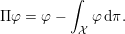 $$\begin{eqnarray}{\rm\Pi}{\it\varphi}={\it\varphi}-\int _{{\mathcal{X}}}{\it\varphi}\,\text{d}{\it\pi}.\end{eqnarray}$$
Note finally that we used the invariance of  ${\it\pi}$ to write
 $\mathbb{E}_{{\it\pi}}\widehat{{\it\varphi}}_{t}=\mathbb{E}_{{\it\pi}}{\it\varphi}$. To prove that (3.2) is indeed well defined, we rewrite it in terms of the semigroup
 $\text{e}^{t{\mathcal{L}}}$. We expand
 $t\,\text{Var}_{{\it\pi}}(\widehat{{\it\varphi}}_{t})$ as
 $$\begin{eqnarray}\displaystyle t\,\text{Var}_{{\it\pi}}(\widehat{{\it\varphi}}_{t}) & = & \displaystyle \frac{1}{t}\int _{0}^{t}\int _{0}^{t}\mathbb{E}_{{\it\pi}}[{\rm\Pi}{\it\varphi}(x_{s}){\rm\Pi}{\it\varphi}(x_{r})]\,\text{d}r\,\text{d}s\nonumber\\ \displaystyle & = & \displaystyle \frac{2}{t}\int _{0}^{t}\int _{0}^{s}\mathbb{E}_{{\it\pi}}[{\rm\Pi}{\it\varphi}(x_{s}){\rm\Pi}{\it\varphi}(x_{r})]\,\text{d}r\,\text{d}s,\nonumber\end{eqnarray}$$
and use the stationarity of the process (valid since the dynamics
is started under the invariant measure  ${\it\pi}$) to write, for
 $s\geqslant r$,
 $$\begin{eqnarray}\mathbb{E}_{{\it\pi}}[{\rm\Pi}{\it\varphi}(x_{s}){\rm\Pi}{\it\varphi}(x_{r})]=\mathbb{E}_{{\it\pi}}[{\rm\Pi}{\it\varphi}(x_{s-r}){\rm\Pi}{\it\varphi}(x_{0})].\end{eqnarray}$$
Then,
 $$\begin{eqnarray}\displaystyle t\,\text{Var}(\widehat{{\it\varphi}}_{t}) & = & \displaystyle 2\int _{0}^{t}\biggl(1-\frac{s}{t}\biggr)\mathbb{E}_{{\it\pi}}[{\rm\Pi}{\it\varphi}(x_{s}){\rm\Pi}{\it\varphi}(x_{0})]\,\text{d}s\nonumber\\ \displaystyle & = & \displaystyle 2\int _{0}^{t}\biggl(1-\frac{s}{t}\biggr)\int _{{\mathcal{X}}}(\text{e}^{s{\mathcal{L}}}{\rm\Pi}{\it\varphi})(x){\rm\Pi}{\it\varphi}(x)\,{\it\pi}(\text{d}x)\,\text{d}s.\nonumber\end{eqnarray}$$
Let us now assume that decay estimates for the semigroup  $\text{e}^{s{\mathcal{L}}}$ are available in a functional space
 $\mathscr{E}\subset L_{0}^{2}({\it\pi})$, typically
 $$\begin{eqnarray}\Vert \text{e}^{s{\mathcal{L}}}\Vert _{{\mathcal{B}}(\mathscr{E})}\leqslant C\,\text{e}^{-{\it\kappa}s},\quad \text{for all }t\geqslant 0,\end{eqnarray}$$
for some positive constants  $C$ and
 ${\it\kappa}$. Various ways of proving such inequalities are provided in
Section 2, with
 $\mathscr{E}$ being
 $L_{0}^{2}({\it\pi})$ (see Propositions 2.3 and 2.20),
 $H^{1}({\it\pi})\cap L_{0}^{2}({\it\pi})$ (see Theorem 2.15) or
 $L_{{\mathcal{K}},0}^{\infty }({\mathcal{X}})$ (see (2.78)). If
 ${\it\varphi}\in \mathscr{E}$, then the dominated convergence theorem shows that
 $$\begin{eqnarray}\lim _{t\rightarrow \infty }t\,\text{Var}_{{\it\pi}}(\widehat{{\it\varphi}}_{t})={\it\varsigma}_{{\it\varphi}}^{2},\end{eqnarray}$$
with
 $$\begin{eqnarray}{\it\varsigma}_{{\it\varphi}}^{2}=2\int _{0}^{+\infty }\int _{{\mathcal{X}}}(\text{e}^{s{\mathcal{L}}}{\rm\Pi}{\it\varphi}){\rm\Pi}{\it\varphi}\,\text{d}{\it\pi}\,\text{d}s=-2\int _{{\mathcal{X}}}({\mathcal{L}}^{-1}{\rm\Pi}{\it\varphi}){\rm\Pi}{\it\varphi}\,\text{d}{\it\pi}.\end{eqnarray}$$
Recall that  ${\mathcal{L}}^{-1}$ is a well-defined bounded operator on
 $\mathscr{E}$ when decay estimates such as (3.4) hold (see Proposition 2.1 and Corollaries 2.4, 2.16, 2.21
and 2.27).
It is instructive at this stage to compare the asymptotic variance (3.5) to the one obtained by
averages of independent and identically distributed (i.i.d.) random variables  $(x^{n})_{n\geqslant 1}$ with common law
 ${\it\pi}$. When
 ${\it\varphi}\in L^{2}({\it\pi})$, a central limit theorem holds true for the estimator
 $$\begin{eqnarray}\widehat{{\it\varphi}}_{N}^{\text{iid}}=\frac{1}{N}\mathop{\sum }_{n=1}^{N}{\it\varphi}(x^{n}),\end{eqnarray}$$
whose asymptotic variance is
 $$\begin{eqnarray}{\it\varsigma}_{{\it\varphi},\text{iid}}^{2}=\lim _{N\rightarrow +\infty }N\mathbb{E}_{{\it\pi}}[(\widehat{{\rm\Pi}{\it\varphi}}_{N}^{\text{iid}})^{2}]=\int _{{\mathcal{X}}}({\rm\Pi}{\it\varphi})^{2}\,\text{d}{\it\pi}.\end{eqnarray}$$
We write the asymptotic variance (3.5) for time average estimates with ergodic SDEs in terms
of the reference variance  ${\it\varsigma}_{{\it\varphi},\text{iid}}^{2}$ as
 $$\begin{eqnarray}{\it\varsigma}_{{\it\varphi}}^{2}={\it\theta}_{\text{corr},{\it\varphi}}{\it\varsigma}_{{\it\varphi},\text{iid}}^{2},\end{eqnarray}$$
and interpret  ${\it\theta}_{\text{corr},{\it\varphi}}$ as some correlation time. Then the mean-square error of the
estimator
 $\widehat{{\it\varphi}}_{t}$ asymptotically behaves as
 ${\it\varsigma}_{{\it\varphi}}^{2}/t={\it\varsigma}_{{\it\varphi},\text{iid}}^{2}{\it\theta}_{\text{corr},{\it\varphi}}/t$, so that in order to have an estimator of the same quality as
that based on
 $N$ i.i.d. samples, integration times of order
 $t=N{\it\theta}_{\text{corr},{\it\varphi}}$ should be considered. When the operator
 ${\mathcal{L}}$ is self-adjoint on
 $L^{2}({\it\pi})$, the norm of
 ${\mathcal{L}}^{-1}$ on
 $L_{0}^{2}({\it\pi})$ is equal to
 $1/{\it\lambda}_{1}$,
 ${\it\lambda}_{1}$ being the first non-zero eigenvalue of
 $-{\mathcal{L}}$ on
 $L^{2}({\it\pi})$ (see the discussion in Section 2.5). This provides the following upper bound for the
correlation time:
 ${\it\theta}_{\text{corr},{\it\varphi}}\leqslant 1/{\it\lambda}_{1}$. Equality holds when
 ${\it\varphi}$ is an eigenvector of
 $-{\mathcal{L}}$ associated with
 ${\it\lambda}_{1}$.
3.1.3 Central Limit Theorems
Note that (3.5) shows that it is
possible to define the asymptotic variance without any reference to the evolution
semigroup  $\text{e}^{t{\mathcal{L}}}$, by directly considering
 $$\begin{eqnarray}{\it\varsigma}_{{\it\varphi}}^{2}=-2\int _{{\mathcal{X}}}({\mathcal{L}}^{-1}{\rm\Pi}{\it\varphi}){\rm\Pi}{\it\varphi}\,\text{d}{\it\pi}.\end{eqnarray}$$
The integral on the right-hand side is well defined once the
solution  ${\rm\Phi}$ of the Poisson equation
 $$\begin{eqnarray}-{\mathcal{L}}{\rm\Phi}={\rm\Pi}{\it\varphi}\end{eqnarray}$$
belongs to a functional space  $\mathscr{E}\subset L^{2}({\it\pi})$. This is the case when
 ${\it\varphi}\in \mathscr{E}$ and
 ${\mathcal{L}}^{-1}$ is a bounded operator on
 $\mathscr{E}$; see the discussion after (3.5). However, there are more
general frameworks to define solutions of Poisson equations; see for instance
Pardoux and Veretennikov (Reference Pardoux and Veretennikov2005) and
references therein.
In fact, it was proved by Bhattacharya (Reference Bhattacharya1982) that a central limit theorem holds once the Poisson equation (3.7) has a solution in  $L^{2}({\it\pi})$ and the initial conditions are distributed according to
 ${\it\pi}$. In this case,
 $$\begin{eqnarray}\lim _{t\rightarrow \infty }\sqrt{t}\,\widehat{{\rm\Pi}{\it\varphi}}_{t}={\mathcal{N}}(0,{\it\varsigma}_{{\it\varphi}}^{2})\text{ in law}.\end{eqnarray}$$
This result can be extended to cover the case when the initial
conditions are not distributed according to the invariant measure: see
also Bhattacharya (Reference Bhattacharya1982). The bottom line
of the proof is to use Itô calculus to rewrite  $\sqrt{t}\,\widehat{{\rm\Pi}{\it\varphi}}_{t}$ as
 $$\begin{eqnarray}\sqrt{t}\,\widehat{{\rm\Pi}{\it\varphi}}_{t}=\frac{{\rm\Phi}(x_{0})-{\rm\Phi}(x_{t})}{\sqrt{t}}+{\mathcal{M}}_{t},\quad {\mathcal{M}}_{t}=\frac{1}{\sqrt{t}}\int _{0}^{t}{\rm\nabla}{\rm\Phi}(x_{s})^{T}{\it\sigma}(x_{s})\,\text{d}W_{s}.\end{eqnarray}$$
The first term converges to 0 in law as  $t\rightarrow +\infty$, while a central limit theorem for martingales can be applied to
obtain the asymptotic behaviour of the second term (see for instance Komorowski,
Landim and Olla Reference Komorowski, Landim and Olla2012 or Ethier and Kurtz
Reference Ethier and Kurtz1986):
 ${\mathcal{M}}_{t}$ converges in law to a Gaussian distribution with variance
 $$\begin{eqnarray}\widetilde{{\it\varsigma}}^{2}=\lim _{t\rightarrow +\infty }\mathbb{E}\biggl(\frac{1}{t}\int _{0}^{t}{\rm\nabla}{\rm\Phi}(x_{s})^{T}{\it\sigma}(x_{s}){\it\sigma}(x_{s})^{T}{\rm\nabla}{\rm\Phi}(x_{s})\,\text{d}s\biggr).\end{eqnarray}$$
By ergodicity of the dynamics,
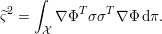 $$\begin{eqnarray}\widetilde{{\it\varsigma}}^{2}=\int _{{\mathcal{X}}}{\rm\nabla}{\rm\Phi}^{T}{\it\sigma}{\it\sigma}^{T}{\rm\nabla}{\rm\Phi}\,\text{d}{\it\pi}.\end{eqnarray}$$
Now, recalling the expression (1.12) for the generator, a simple computation shows that
 $$\begin{eqnarray}{\mathcal{L}}({\rm\Phi}^{2})-2{\rm\Phi}{\mathcal{L}}{\rm\Phi}={\it\sigma}{\it\sigma}^{T}:{\rm\nabla}^{2}({\rm\Phi}^{2})-2{\rm\Phi}{\it\sigma}{\it\sigma}^{T}:{\rm\nabla}^{2}{\rm\Phi}={\rm\nabla}{\rm\Phi}^{T}{\it\sigma}{\it\sigma}^{T}{\rm\nabla}{\rm\Phi}.\end{eqnarray}$$
The invariance of  ${\it\pi}$, expressed as (1.17), then leads to
 $$\begin{eqnarray}\widetilde{{\it\varsigma}}^{2}=\int _{{\mathcal{X}}}{\rm\nabla}{\rm\Phi}^{T}{\it\sigma}{\it\sigma}^{T}{\rm\nabla}{\rm\Phi}\,\text{d}{\it\pi}=-2\int _{{\mathcal{X}}}{\rm\Phi}{\mathcal{L}}{\rm\Phi}\,\text{d}{\it\pi}={\it\varsigma}_{{\it\varphi}}^{2},\end{eqnarray}$$
which allows us to conclude.
3.2 Numerical discretizations and their ergodic behaviour
In practice, continuous dynamics such as (3.1) are discretized in time using a numerical scheme. The simplest choice
is to resort to an Euler–Maruyama discretization with a fixed time step  ${\rm\Delta}t>0$. In this case
 $x_{n{\rm\Delta}t}$ is approximated by
 $x^{n}$, constructed iteratively from a given initial condition
 $x^{0}=x_{0}$ as
 $$\begin{eqnarray}x^{n+1}=x^{n}+b(x^{n})\,{\rm\Delta}t+{\it\sigma}(x^{n})\sqrt{{\rm\Delta}t}\,G^{n},\end{eqnarray}$$
where  $G^{n}$ is a sequence of i.i.d. Gaussian random variables with
covariance matrix
 $\text{Id}_{d}$. Hereafter, the evolution operator (also called the transition
operator) associated with a general one-step numerical scheme is
denoted by
 $$\begin{eqnarray}P_{{\rm\Delta}t}{\it\varphi}(x)=\mathbb{E}({\it\varphi}(x^{n+1})\mid x^{n}=x).\end{eqnarray}$$
It is the discrete counterpart of the semigroup  $\text{e}^{{\rm\Delta}t{\mathcal{L}}}$. The transition operator
 $P_{{\rm\Delta}t}$ describes how the values of a given function evolve on average over
one time step.
We discuss in this section the various types of errors arising from the time discretization. We first recall the standard measures of error on finite time intervals (weak versus strong errors). We then turn to our main concern, error estimates on long time averages. As discussed below, these errors can be decomposed, for sufficiently long times, into (i) a systematic part, related to errors on the invariant measure due to the time discretization, and (ii) a statistical error dictated by a central limit theorem, with an asymptotic variance close to that of the underlying continuous process. The quality of the numerical schemes for ergodic dynamics is therefore mainly determined by the size of the systematic errors, as well as their stability.
3.2.1 Standard numerical analysis of SDEs
There are many good review articles and textbooks on the numerical analysis of SDEs, such as Kloeden and Platen (Reference Kloeden and Platen1992), Platen (Reference Platen1999) and Milstein and Tretyakov (Reference Milstein and Tretyakov2004). Two types of errors are considered for discretizations of SDEs, as follows.
(i) Weak error estimates. There exists
${\it\alpha}>0$ such that, for any $C^{\infty }$ test function with compact support ${\it\varphi}$ and finite time horizon $T>0$, there are $C\geqslant 0$ and ${\rm\Delta}t^{\ast }>0$ (the latter two constants depending on ${\it\varphi}$ and $T$ a priori) such that, for any ${\rm\Delta}t\in (0,{\rm\Delta}t^{\ast }]$, In fact, when the numerical method is stable (which is the case when$$\begin{eqnarray}\sup _{0\leqslant n\leqslant T/{\rm\Delta}t}|\mathbb{E}[{\it\varphi}(x^{n})]-\mathbb{E}[{\it\varphi}(x_{n{\rm\Delta}t})]|\leqslant C{\rm\Delta}t^{{\it\alpha}}.\end{eqnarray}$$$b$ and ${\it\sigma}$ are globally Lipschitz), such error estimates can be
deduced from the error over one time step, as stated in
Theorem 2.1 of Milstein and Tretyakov (Reference Milstein and Tretyakov2004). In essence, the order ${\it\alpha}$ is determined by the formal equality To make the functional setting more precise, this should be understood as$$\begin{eqnarray}P_{{\rm\Delta}t}=\text{e}^{{\rm\Delta}t{\mathcal{L}}}+\text{O}({\rm\Delta}t^{{\it\alpha}+1}).\end{eqnarray}$$$P_{{\rm\Delta}t}{\it\varphi}=\text{e}^{{\rm\Delta}t{\mathcal{L}}}{\it\varphi}+{\rm\Delta}t^{{\it\alpha}+1}r_{{\it\varphi},{\rm\Delta}t}$ for a function ${\it\varphi}$ growing at most polynomially, whose derivatives of
order at most $2{\it\alpha}+2$ grow at most polynomially, and with a remainder term $r_{{\it\varphi},{\rm\Delta}t}$ such that there exists $p\in \mathbb{N}$ for which $\Vert r_{{\it\varphi},{\rm\Delta}t}/(1+|x|^{p})\Vert _{L^{\infty }}\leqslant K$, for ${\rm\Delta}t$ sufficiently small.(ii) Strong error estimates in
$L^{p}$-norm. There exists ${\it\alpha}\in \mathbb{R}_{+}$ such that, for any time horizon $T$, there is $C\geqslant 0$ and ${\rm\Delta}t^{\ast }>0$ (the latter two constants depending on $T$ a priori) such that, for any $0\leqslant {\rm\Delta}t\leqslant {\rm\Delta}t^{\ast }$, In this case the Gaussian increments used in a numerical scheme such as (3.8) must be induced by the Brownian motion for the continuous dynamics (3.1), that is,$$\begin{eqnarray}\sup _{0\leqslant n\leqslant T/{\rm\Delta}t}(\mathbb{E}|x^{n}-x_{n{\rm\Delta}t}|^{p})^{1/p}\leqslant C{\rm\Delta}t^{{\it\alpha}}.\end{eqnarray}$$$$\begin{eqnarray}G^{n}=\frac{W_{(n+1){\rm\Delta}t}-W_{n{\rm\Delta}t}}{\sqrt{{\rm\Delta}t}}.\end{eqnarray}$$








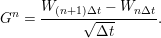
Typically, the constant  $C$ is obtained via some (discrete) Gronwall estimate, as in the
standard numerical analysis of ordinary differential equations, and hence
increases exponentially with time.
As an example, let us mention that, when the functions  $b$ and
 ${\it\sigma}$ in (3.1) are
globally Lipschitz, the weak and strong errors of the Euler–Maruyama
scheme (3.8) are
respectively 1 and 1/2.
Note that it is also possible to reduce errors due to time discretization by resorting to extrapolation methods as in Lamberton and Pagès (Reference Lamberton and Pagès2002) or multilevel Monte Carlo methods (Giles Reference Giles2008, Giles Reference Giles2015).
3.2.2 Convergence of time averages
The above error estimates are not relevant to long-time convergence since the prefactor  $C$ is not uniformly controlled in time. Therefore, additional
techniques should be introduced to control the quality of the approximation of
average properties presented by the time averages traditionally considered in
molecular simulation:
 $$\begin{eqnarray}\widehat{{\it\varphi}}_{N_{\text{iter}},{\rm\Delta}t}=\frac{1}{N_{\text{ter}}}\mathop{\sum }_{n=0}^{N_{\text{iter}}-1}{\it\varphi}(x^{n}).\end{eqnarray}$$
A first issue is to prove that the numerical scheme is indeed ergodic with respect
to some probability measure, which depends in general on the time step  ${\rm\Delta}t$. Even if the associated continuous dynamics is ergodic, the
ergodicity of the discretized dynamics cannot be guaranteed. A typical obstruction
is the presence of non-globally Lipschitz drifts which induce a transient
behaviour of the Markov chain; see for instance the examples provided in Mattingly
et al. (Reference Mattingly, Stuart and Higham2002, Section 6.3) for
 $b(x)=-x^{3}$ and
 ${\it\sigma}(x)=1$.
In order to prove the existence of an invariant probability measure  ${\it\pi}_{{\rm\Delta}t}$ for the numerical scheme, it is standard to resort to results
such as Theorem 2.25.
Proving that a minorization condition holds on any compact set (see
Assumption 2.24) is
usually not too difficult, thanks to the presence of Gaussian increments; see for
instance Lemma 3.4 below
for an Euler–Maruyama discretization of the overdamped Langevin
dynamics. Some assumptions on the drift, on the other hand, are usually required
to state a Lyapunov condition such as (2.62): see Mattingly
et al. (Reference Mattingly, Stuart and Higham2002).
When these conditions are met, the convergence of the law of
 $x^{n}$ to the invariant measure is exponentially fast (with respect to
the iteration index, the time step
 ${\rm\Delta}t$ being fixed, as stated in Theorem 2.25).
The next step is to prove that the numerical scheme is irreducible. Usually,
irreducibility is defined with respect to the Lebesgue measure, in which case this
property reads: for any Borel subset  $S\subset {\mathcal{X}}$ of positive Lebesgue measure, and any initial condition
 $x^{0}\in {\mathcal{X}}$, we have
 $\mathbb{P}_{x^{0}}({\it\tau}_{S}<+\infty )>0$, where
 ${\it\tau}_{S}=\inf \{n\geqslant 0,x^{n}\in S\}$ is the first entry time into the set
 $S$. Note that
 $\mathbb{P}_{x^{0}}({\it\tau}_{S}<+\infty )>0$ is implied by the following property: for any Borel subset
 $S\subset {\mathcal{X}}$ of positive Lebesgue measure and any initial condition
 $x^{0}\in {\mathcal{X}}$, there exists
 $n\geqslant 0$ (depending on
 $x^{0}$ and
 $S$) such that
 $P^{n}(x^{0},S)>0$. For discretizations of SDEs, the latter inequality is often
easy to establish. It holds, for instance, with
 $n=1$ for the Euler–Maruyama scheme (3.8) when
 ${\it\sigma}$ has full rank
 $d$ at each point
 $x\in {\mathcal{X}}$, since
 $$\begin{eqnarray}G^{1}={\it\sigma}(x^{0})^{-1}\biggl(\displaystyle \frac{x^{1}-x^{0}-{\rm\Delta}t\,b(x^{0})}{\sqrt{{\rm\Delta}t}}\biggr)=:{\mathcal{G}}_{x^{0}}(x^{1}),\end{eqnarray}$$
so that
 $$\begin{eqnarray}P(x^{0},S)=\mathbb{P}(G^{1}\in {\mathcal{G}}_{x_{0}}^{-1}(S))>0.\end{eqnarray}$$
When  ${\it\sigma}$ is degenerate, several iterates may be necessary; see for
instance Bou-Rabee and Owhadi (Reference Bou-Rabee and Owhadi2010), where
it is proved that
 $P^{2}(x^{0},S)>0$ for some discretization of Langevin dynamics.
Once the existence of an invariant probability measure and the irreducibility of
the scheme are proved, the almost-sure convergence of long-time averages over one
realization already follows (see Chapter 17 in Meyn and Tweedie (Reference Meyn and Tweedie2009)): for almost all initial conditions  $x^{0}\in {\mathcal{X}}$,
 $$\begin{eqnarray}\widehat{{\it\varphi}}_{N_{\text{iter}},{\rm\Delta}t}\xrightarrow[N_{\text{iter}}\rightarrow +\infty ]{\text{a.s.}}\int _{{\mathcal{X}}}{\it\varphi}\,\text{d}{\it\pi}_{{\rm\Delta}t}.\end{eqnarray}$$
Let us also mention that, when irreducibility holds with respect
to the Lebesgue measure, the measure  ${\it\pi}_{{\rm\Delta}t}$ is absolutely continuous with respect to the Lebesgue measure.
In addition, when the transition kernel
 $P(x,\text{d}y)$ is absolutely continuous with respect to the Lebesgue measure
 $\text{d}y$, the above almost sure convergence occurs for all initial
conditions: see Corollary 1 in Tierney (Reference Tierney1994), based on Nummelin (Reference Nummelin1984).
As in the continuous case, when decay estimates on the evolution operator  $P_{{\rm\Delta}t}$ hold as in Theorem 2.25, it can easily be shown that the asymptotic variance
is well defined when
 $x^{0}\sim {\it\pi}_{{\rm\Delta}t}$, provided
 ${\mathcal{K}}\in L^{2}({\it\pi}_{{\rm\Delta}t})$ and
 ${\it\varphi}\in L_{{\mathcal{K}}}^{\infty }({\mathcal{X}})$. A way to prove that
 ${\mathcal{K}}\in L^{2}({\it\pi}_{{\rm\Delta}t})$ is to check whether the assumptions of Theorem 2.25 are satisfied for the Lyapunov
function
 ${\mathcal{K}}^{2}$ instead of
 ${\mathcal{K}}$, so that the integrability condition follows
from (2.64). In
practice, it is often convenient to establish minorization conditions on arbitrary
compact sets, and to obtain Lyapunov conditions for the family of functions
 ${\mathcal{K}}_{n}(x)=1+|x|^{n}$ (for integers
 $n\geqslant n_{0}$ sufficiently large). Note that
 ${\mathcal{K}}_{n}^{2}={\mathcal{K}}_{2n}+2({\mathcal{K}}_{n}-1)$, so that the
 $L^{2}({\it\pi}_{{\rm\Delta}t})$ integrability of
 ${\mathcal{K}}_{n}$ follows once Lyapunov estimates hold for
 ${\mathcal{K}}_{2n}$.
To state the expression of the asymptotic variance when Theorem 2.25 holds for a Lyapunov function  ${\mathcal{K}}\in L^{2}({\it\pi}_{{\rm\Delta}t})$, let us introduce the equivalent of the projection
operator (3.3) for
the invariant measure
 ${\it\pi}_{{\rm\Delta}t}$, namely
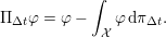 $$\begin{eqnarray}{\rm\Pi}_{{\rm\Delta}t}{\it\varphi}={\it\varphi}-\int _{{\mathcal{X}}}{\it\varphi}\,\text{d}{\it\pi}_{{\rm\Delta}t}.\end{eqnarray}$$
Note that if  $x^{0}\sim {\it\pi}_{{\rm\Delta}t}$, then
 $x^{n}\sim {\it\pi}_{{\rm\Delta}t}$ for all
 $n\geqslant 1$ and the following stationarity property holds:
 $$\begin{eqnarray}\mathbb{E}_{{\it\pi}_{{\rm\Delta}t}}[{\rm\Pi}_{{\rm\Delta}t}{\it\varphi}(x^{n}){\rm\Pi}_{{\rm\Delta}t}{\it\varphi}(x^{m})]=\mathbb{E}_{{\it\pi}_{{\rm\Delta}t}}[{\rm\Pi}_{{\rm\Delta}t}{\it\varphi}(x^{|n-m|}){\rm\Pi}_{{\rm\Delta}t}{\it\varphi}(x^{0})]\end{eqnarray}$$
for all  $n,m\geqslant 0$. Then,
 $$\begin{eqnarray}\displaystyle & & \displaystyle N_{\text{iter}}\,\text{Var}_{{\it\pi}_{{\rm\Delta}t}}(\widehat{{\it\varphi}}_{N_{\text{iter}}})=N_{\text{iter}}\,\mathbb{E}_{{\it\pi}_{{\rm\Delta}t}}[({\rm\Pi}_{{\rm\Delta}t}\widehat{{\it\varphi}}_{N_{\text{iter}}})^{2}]\nonumber\\ \displaystyle & & \displaystyle \quad ~\;=\frac{1}{N_{\text{iter}}}\mathop{\sum }_{n,m=0}^{N_{\text{iter}}-1}\mathbb{E}_{{\it\pi}_{{\rm\Delta}t}}[{\rm\Pi}_{{\rm\Delta}t}{\it\varphi}(x^{n}){\rm\Pi}_{{\rm\Delta}t}{\it\varphi}(x^{m})]\nonumber\\ \displaystyle & & \displaystyle \quad ~\;=\frac{1}{N_{\text{iter}}}\mathop{\sum }_{n=0}^{N_{\text{iter}}-1}\mathbb{E}_{{\it\pi}_{{\rm\Delta}t}}[({\rm\Pi}_{{\rm\Delta}t}{\it\varphi}(x^{n}))^{2}]\nonumber\\ \displaystyle & & \displaystyle \quad ~\;\qquad +\frac{2}{N_{\text{iter}}}\mathop{\sum }_{0\leqslant m<n\leqslant N_{\text{iter}}-1}\mathbb{E}_{{\it\pi}_{{\rm\Delta}t}}[{\rm\Pi}_{{\rm\Delta}t}{\it\varphi}(x^{n}){\rm\Pi}_{{\rm\Delta}t}{\it\varphi}(x^{m})]\nonumber\\ \displaystyle & & \displaystyle \quad ~\;=\mathbb{E}_{{\it\pi}_{{\rm\Delta}t}}[({\rm\Pi}_{{\rm\Delta}t}{\it\varphi})^{2}]+2\mathop{\sum }_{1\leqslant n\leqslant N_{\text{iter}}-1}\!\biggl(1-\displaystyle \frac{n}{N_{\text{iter}}}\biggr)\mathbb{E}_{{\it\pi}_{{\rm\Delta}t}}[{\rm\Pi}_{{\rm\Delta}t}{\it\varphi}(x^{n}){\rm\Pi}_{{\rm\Delta}t}{\it\varphi}(x^{0})],\nonumber\end{eqnarray}$$
where we used the stationarity property in the last step. Since
 $$\begin{eqnarray}\mathbb{E}_{{\it\pi}_{{\rm\Delta}t}}[{\rm\Pi}_{{\rm\Delta}t}{\it\varphi}(x^{n}){\rm\Pi}_{{\rm\Delta}t}{\it\varphi}(x^{0})]=\int _{{\mathcal{X}}}({\rm\Pi}_{{\rm\Delta}t}{\it\varphi})(P_{{\rm\Delta}t}^{n}{\rm\Pi}_{{\rm\Delta}t}{\it\varphi})\,\text{d}{\it\pi}_{{\rm\Delta}t},\end{eqnarray}$$
and we assume (2.67) to hold, a dominated convergence argument shows that
 $$\begin{eqnarray}\lim _{N_{\text{iter}}\rightarrow +\infty }N_{\text{iter}}\text{Var}_{{\it\pi}_{{\rm\Delta}t}}(\widehat{{\it\varphi}}_{N_{\text{iter}},{\rm\Delta}t})={\it\varsigma}_{{\it\varphi},{\rm\Delta}t}^{2}\end{eqnarray}$$
with (compare with (3.5))
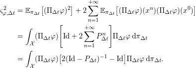 $$\begin{eqnarray}\displaystyle {\it\varsigma}_{{\it\varphi},{\rm\Delta}t}^{2} & = & \displaystyle \mathbb{E}_{{\it\pi}_{{\rm\Delta}t}}[({\rm\Pi}_{{\rm\Delta}t}{\it\varphi})^{2}]+2\mathop{\sum }_{n=1}^{+\infty }\mathbb{E}_{{\it\pi}_{{\rm\Delta}t}}[({\rm\Pi}_{{\rm\Delta}t}{\it\varphi})(x^{n})({\rm\Pi}_{{\rm\Delta}t}{\it\varphi})(x^{0})]\nonumber\\ \displaystyle & = & \displaystyle \int _{{\mathcal{X}}}({\rm\Pi}_{{\rm\Delta}t}{\it\varphi})\left[\text{Id}+2\mathop{\sum }_{n=1}^{+\infty }P_{{\rm\Delta}t}^{n}\right]{\rm\Pi}_{{\rm\Delta}t}{\it\varphi}\,\text{d}{\it\pi}_{{\rm\Delta}t}\nonumber\\ \displaystyle & = & \displaystyle \int _{{\mathcal{X}}}({\rm\Pi}_{{\rm\Delta}t}{\it\varphi})[2(\text{Id}-P_{{\rm\Delta}t})^{-1}-\text{Id}]{\rm\Pi}_{{\rm\Delta}t}{\it\varphi}\,\text{d}{\it\pi}_{{\rm\Delta}t}.\end{eqnarray}$$
The expression for the asymptotic variance suggests a definition of a correlation time, as for continuous dynamics. By the same reasoning as in (3.6), using the variance obtained with i.i.d. samples as a reference,
 $$\begin{eqnarray}{\it\varsigma}_{{\it\varphi},{\rm\Delta}t}^{2}=N_{\text{corr},{\rm\Delta}t,{\it\varphi}}{\it\varsigma}_{{\it\varphi},\text{iid},{\rm\Delta}t}^{2}\quad \text{where }{\it\varsigma}_{{\it\varphi},\text{iid},{\rm\Delta}t}^{2}=\int _{{\mathcal{X}}}({\rm\Pi}_{{\rm\Delta}t}{\it\varphi})^{2}\,\text{d}{\it\pi}_{{\rm\Delta}t}.\end{eqnarray}$$
The number  $N_{\text{corr},{\rm\Delta}t,{\it\varphi}}$ measures the correlation between the samples: intuitively, it
gives the number of steps which should be performed to have a new configuration
sufficiently decorrelated from the previous one. As discussed below, the
correlation time
 ${\it\theta}_{\text{corr},{\it\varphi}}$ is related to the number of correlation steps
 $N_{\text{corr},{\rm\Delta}t,{\it\varphi}}$ for the discrete dynamics since in the limit of small
 ${\rm\Delta}t$,
 ${\it\theta}_{\text{corr},{\it\varphi}}\simeq N_{\text{corr},{\rm\Delta}t,{\it\varphi}}{\rm\Delta}t$.
Finally, let us mention that, as in the continuous case, a central limit theorem
in fact holds true for time averages computed using ergodic Markov chains once the
solution  ${\rm\Phi}$ of the Poisson equation
 $$\begin{eqnarray}(\text{Id}-P_{{\rm\Delta}t}){\rm\Phi}={\rm\Pi}_{{\rm\Delta}t}{\it\varphi}\end{eqnarray}$$
belongs to  $L^{2}({\it\pi}_{{\rm\Delta}t})$; see Theorem 17.4.4 in Meyn and Tweedie (Reference Meyn and Tweedie2009). If
 ${\it\varphi}\in L_{{\mathcal{K}}}^{\infty }({\mathcal{X}})$ and
 ${\mathcal{K}}\in L^{2}({\it\pi}_{{\rm\Delta}t})$ (see the above discussion for the latter condition), one way to
guarantee that
 ${\rm\Phi}\in L^{2}({\it\pi}_{{\rm\Delta}t})$ is to resort to Corollary 2.26.
3.2.3 Error analysis on time averages: general decomposition
Let us now discuss the topic of main interest for this section, namely error
estimates for the computation of thermodynamic averages  $\mathbb{E}_{{\it\pi}}({\it\varphi})=\int _{{\mathcal{X}}}{\it\varphi}\,\text{d}{\it\pi}$ with (3.10),
for a given one-step discretization of the continuous dynamics (3.1) ergodic with respect to
 ${\it\pi}$. We decompose the error as the sum of two contributions:
 $$\begin{eqnarray}\widehat{{\it\varphi}}_{N_{\text{iter}},{\rm\Delta}t}-\mathbb{E}_{{\it\pi}}({\it\varphi})=(\widehat{{\it\varphi}}_{N_{\text{iter}},{\rm\Delta}t}-\mathbb{E}_{{\it\pi}_{{\rm\Delta}t}}({\it\varphi}))+(\mathbb{E}_{{\it\pi}_{{\rm\Delta}t}}({\it\varphi})-\mathbb{E}_{{\it\pi}}({\it\varphi})).\end{eqnarray}$$
The first term is a statistical error arising from the finiteness
of the number of time steps  $N_{\text{iter}}$, while the second term is a systematic error (or bias), which
persists in the limit
 $N_{\text{iter}}\rightarrow +\infty$, and is due to the use of finite time steps
 ${\rm\Delta}t>0$. Let us discuss each term more precisely.
(i) According to the central limit theorem for Markov chains (which holds when the Poisson equation (3.12) can be solved in
$L^{2}({\it\pi}_{{\rm\Delta}t})$: see the above discussion), the statistical
error behaves in the limit $N_{\text{iter}}\rightarrow +\infty$ as a Gaussian random variable with asymptotic variance
given by (3.11). In practice, this asymptotic regime is attained when $N_{\text{iter}}\gg N_{\text{corr},{\rm\Delta}t,{\it\varphi}}$. However, $N_{\text{corr},{\rm\Delta}t,{\it\varphi}}$ is often very large because of the metastability of the
underlying continuous dynamics (so that ${\it\theta}_{\text{corr},{\it\varphi}}$ is large), which makes it difficult in practice to
ensure that the central limit theorem actually holds for the values of $N_{\text{iter}}$ achievable with computer simulations.When the asymptotic regime can be considered to have been attained,
$\widehat{{\it\varphi}}_{N_{\text{iter}},{\rm\Delta}t}-\mathbb{E}_{{\it\pi}_{{\rm\Delta}t}}({\it\varphi})$ is of order This reformulation highlights the fact that the statistical error is of the order of the inverse of the square root of the ‘physical’ simulation time$$\begin{eqnarray}\frac{{\it\varsigma}_{{\it\varphi},{\rm\Delta}t}}{\sqrt{N_{\text{iter}}}}=\frac{{\it\varsigma}_{{\it\varphi},{\rm\Delta}t}\sqrt{{\rm\Delta}t}}{\sqrt{T}}.\end{eqnarray}$$$T=N_{\text{iter}}{\rm\Delta}t$. Indeed, weakly consistent discretizations of SDEs are
such that In addition, the variance$$\begin{eqnarray}\frac{\text{Id}-P_{{\rm\Delta}t}}{{\rm\Delta}t}{\it\varphi}=-{\mathcal{L}}{\it\varphi}+\text{O}({\rm\Delta}t).\end{eqnarray}$$${\it\varsigma}_{{\it\varphi},{\rm\Delta}t}^{2}$ can be rewritten as In view of the expression$$\begin{eqnarray}{\rm\Delta}t\,{\it\varsigma}_{{\it\varphi},{\rm\Delta}t}^{2}=2\int _{{\mathcal{X}}}({\rm\Pi}_{{\rm\Delta}t}{\it\varphi})\biggl(\frac{\text{Id}-P_{{\rm\Delta}t}}{{\rm\Delta}t}\biggr)^{-1}{\rm\Pi}_{{\rm\Delta}t}{\it\varphi}\,\text{d}{\it\pi}_{{\rm\Delta}t}+\text{O}({\rm\Delta}t).\end{eqnarray}$$${\it\varsigma}_{{\it\varphi}}^{2}$ of the asymptotic variance (3.5) of the continuous
dynamics, this suggests the following convergence result: (3.14)A rigorous proof of this convergence is provided by Theorem 5.6. In fact, it typically holds that$$\begin{eqnarray}\lim _{{\rm\Delta}t\rightarrow 0}{\rm\Delta}t\,{\it\varsigma}_{{\it\varphi},{\rm\Delta}t}^{2}={\it\varsigma}_{{\it\varphi}}^{2}.\end{eqnarray}$$${\it\theta}_{\text{corr},{\it\varphi}}=N_{\text{corr},{\rm\Delta}t,{\it\varphi}}{\rm\Delta}t+\text{O}({\rm\Delta}t)$.The interpretation of (3.14) is that the asymptotic variance of time averages computed using numerical methods is, to first order in
${\rm\Delta}t$, related to the asymptotic variance of the time
averages computed with the continuous process. This motivates direct
study of the variance (3.5) rather than its discrete counterpart, which we therefore do
in Section 3.4.(ii) The second term in (3.13) is a systematic error (or bias) related to the fact that the invariant measure of the numerical scheme
${\it\pi}_{{\rm\Delta}t}$ is different from the canonical measure ${\it\pi}$. Although this is not obvious, the expression of the
formal correction function $h_{{\rm\Delta}t}$ defined as ${\it\pi}_{{\rm\Delta}t}=h_{{\rm\Delta}t}{\it\pi}$ is encoded in the asymptotic expansion of the one-step
evolution operator $P_{{\rm\Delta}t}$, provided some ergodicity conditions are met. A typical
result is that $h_{{\rm\Delta}t}=1+\text{O}({\rm\Delta}t^{p})$ for some integer $p$. In fact, it is often possible to make the leading term
in the bias precise as follows (see Theorem 3.3 below): for some function$$\begin{eqnarray}\int _{{\mathcal{X}}}{\it\varphi}\,\text{d}{\it\pi}_{{\rm\Delta}t}=\int _{{\mathcal{X}}}{\it\varphi}\,\text{d}{\it\pi}+{\rm\Delta}t^{p}\int _{{\mathcal{X}}}{\it\varphi}f\,\text{d}{\it\pi}+\text{O}({\rm\Delta}t^{p+1})\end{eqnarray}$$$f$ to be made precise. As made clear in
Theorem 3.3, $p\geqslant {\it\alpha}$, where ${\it\alpha}$ is the weak order of the method (in the sense that $P_{{\rm\Delta}t}=\text{e}^{{\rm\Delta}t{\mathcal{L}}}+\text{O}({\rm\Delta}t^{{\it\alpha}+1})$). In some cases, it even holds that $p\geqslant {\it\alpha}+1$.



















An important remark is that the bias becomes noticeable only for sufficiently long
integration times  $T=N_{\text{iter}}{\rm\Delta}t$, namely when
 ${\it\varsigma}_{{\it\varphi}}/\sqrt{T}\sim {\rm\Delta}t^{p}$. More precisely,
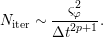 $$\begin{eqnarray}N_{\text{iter}}\sim \frac{{\it\varsigma}_{{\it\varphi}}^{2}}{{\rm\Delta}t^{2p+1}}.\end{eqnarray}$$
This motivates the fact that the statistical error often dominates in actual simulations. However, it is desirable to have biases as small as possible in order to use larger time steps (while still satisfying stability constraints). We now analyse the bias in the next section.
3.3 Analysis of the bias
In this section we present the analysis of the bias (second term on the right-hand side of (3.13)). We start with a presentation of the general strategy, and then apply it to the estimation of canonical averages with discretizations of overdamped Langevin or Langevin dynamics.
3.3.1 General strategy
Assume that the continuous dynamics, with generator  ${\mathcal{L}}$, admits a unique invariant measure
 ${\it\pi}$. Consider next a given numerical scheme, described in terms of
its discrete evolution operator
 $P_{{\rm\Delta}t}$ defined in (3.9), and admitting an invariant measure
 ${\it\pi}_{{\rm\Delta}t}$ (we do not make any uniqueness assumption on
 ${\it\pi}_{{\rm\Delta}t}$ at this stage).
Assume that, for a  $C^{\infty }$ function
 ${\it\varphi}$ and a given integer
 $p$, the evolution operator can be expanded as
 $$\begin{eqnarray}P_{{\rm\Delta}t}{\it\varphi}={\it\varphi}+{\rm\Delta}t\,{\mathcal{A}}_{1}{\it\varphi}+{\rm\Delta}t^{2}{\mathcal{A}}_{2}{\it\varphi}+\cdots +{\rm\Delta}t^{p+1}{\mathcal{A}}_{p+1}{\it\varphi}+{\rm\Delta}t^{p+2}r_{{\it\varphi},{\rm\Delta}t},\end{eqnarray}$$
for some remainder term  $r_{{\it\varphi},{\rm\Delta}t}$ (which depends on
 $p$, although we henceforth omit this dependence). The operators
 ${\mathcal{A}}_{k}$ are identified in practice by Taylor expansions of
 ${\it\varphi}(x^{n+1})$ around
 ${\it\varphi}(x^{n})$, with a remainder term typically expressed as an integral. Note
that, by consistency of the discretization, it typically holds that
 $$\begin{eqnarray}{\mathcal{A}}_{1}={\mathcal{L}},\end{eqnarray}$$
although in principle it is possible to construct numerical
schemes approximating  ${\it\pi}$ for which this is not the case. More generally, the method is of
weak order
 $p$ when
 ${\mathcal{A}}_{k}={\mathcal{L}}^{k}/k!$ for
 $1\leqslant k\leqslant p$. However, there may be discrete dynamics for which
 ${\mathcal{A}}_{k}=a_{k}{\mathcal{L}}^{k}$ with a prefactor
 $a_{k}\neq 1/k!$ for some
 $1\leqslant k\leqslant p$. In this case the dynamics is not of weak order
 $p$, but the invariant measure may nonetheless be correct up to
error terms of order
 ${\rm\Delta}t^{p+1}$. Moreover, as made precise in Theorem 3.3, there are situations in which the
operators
 ${\mathcal{A}}_{k}$ are different from
 ${\mathcal{L}}^{k}$ but the invariant measure
 ${\it\pi}_{{\rm\Delta}t}$ is still close to
 ${\it\pi}$; see for instance Abdulle, Vilmart and Zygalakis (Reference Abdulle, Vilmart and Zygalakis2015) in the context of Langevin dynamics.
We next need some functional estimates on the operator  ${\mathcal{A}}_{1}$ appearing in (3.15). To this end, we introduce the following set of
 $C^{\infty }$ functions.
Definition 3.1 (smooth functions).
Consider scale functions  ${\mathcal{K}}_{n}:{\mathcal{X}}\rightarrow [1,+\infty )$ such that
 $$\begin{eqnarray}{\mathcal{K}}_{n}\leqslant {\mathcal{K}}_{n+1},\quad \text{for all }n\geqslant 0.\end{eqnarray}$$
The space  ${\mathcal{S}}$ is composed of all functions
 ${\it\varphi}\in C^{\infty }({\mathcal{X}})$ for which, for any
 $k\in \mathbb{N}^{d}$, there exists
 $m\in \mathbb{N}$ such that
 $\partial ^{k}{\it\varphi}\in L_{{\mathcal{K}}_{m}}^{\infty }({\mathcal{X}})$.
In the simple case when  ${\mathcal{X}}$ is bounded, it is possible to choose
 ${\mathcal{K}}_{n}=\mathbf{1}$ for all
 $n\geqslant 0$, in which case
 ${\mathcal{S}}=C^{\infty }({\mathcal{X}})$. For unbounded spaces, a typical choice is
 ${\mathcal{K}}_{n}(x)=1+|x|^{n}$. In this case, the above definition means that the functions in
 ${\mathcal{S}}$, as well as all their derivatives, grow at most polynomially.
The set
 ${\mathcal{S}}$ can then be shown to be dense in
 $L^{2}({\it\pi})$ when
 ${\it\pi}$ has moments of all orders, so that all the operators arising in
the error estimations can be considered as operators on
 $L^{2}({\it\pi})$, defined on the core
 ${\mathcal{S}}$.
In order to state the regularity result we rely on, we restrict the space of
smooth functions to those with average 0 with respect to the invariant measure  ${\it\pi}$ of the continuous process, namely
 $$\begin{eqnarray}{\mathcal{S}}_{0}={\rm\Pi}{\mathcal{S}}=\biggl\{{\it\varphi}\in {\mathcal{S}}\,\bigg|\,\int _{{\mathcal{X}}}{\it\varphi}\,\text{d}{\it\pi}=0\biggr\},\end{eqnarray}$$
where  ${\rm\Pi}$ is defined in (3.3). We next consider the following assumption on the generator of the
continuous dynamics. Recall that operators are considered on
 $L^{2}({\it\pi})$ and that adjoints are taken with respect to the corresponding
scalar product.
Assumption 3.2 (stability of smooth functions by inverse operators).
The space  ${\mathcal{S}}$ is dense in
 $L^{2}({\it\pi})$ (in particular
 ${\mathcal{K}}_{n}\in L^{2}({\it\pi})$ for any
 $n\geqslant 0$) and the operators
 ${\mathcal{A}}_{1}^{-1}$ and
 $({\mathcal{A}}_{1}^{\ast })^{-1}$ leave
 ${\mathcal{S}}_{0}$ invariant.
Let us recall that  ${\mathcal{A}}_{1}^{\ast }$ denotes the adjoint of
 ${\mathcal{A}}_{1}$ with respect to the scalar product in
 $L^{2}({\it\mu})$ (see (2.7) and
Section 2.3.2) and that
typically
 ${\mathcal{A}}_{1}={\mathcal{L}}$. The invariance of
 ${\mathcal{S}}_{0}$ by an operator
 ${\mathcal{T}}^{-1}$ has to be understood in the following sense: when
 ${\it\varphi}\in {\mathcal{S}}_{0}$, the unique solution
 ${\rm\Phi}$ of the equation
 ${\mathcal{T}}{\rm\Phi}={\it\varphi}$ belongs to
 ${\mathcal{S}}_{0}$.
Error estimates on averages of smooth functions can finally be stated as follows.
Theorem 3.3 (error estimates on the invariant measure).
Suppose that Assumption 3.2 is satisfied, and that an expansion such as (3.15) holds for any  ${\it\varphi}\in {\mathcal{S}}$ and a given
 $p\in \mathbb{N}$, with a remainder
 $r_{{\it\varphi},{\rm\Delta}t}$ for which there exist
 $K\geqslant 0$,
 $m\in \mathbb{N}$ and
 ${\rm\Delta}t^{\ast }>0$ (all depending on
 ${\it\varphi}$ and
 $p$) such that
 $$\begin{eqnarray}\Vert r_{{\it\varphi},{\rm\Delta}t}\Vert _{L_{{\mathcal{K}}_{m}}^{\infty }}\leqslant K,\quad \text{for all }{\rm\Delta}t\leqslant {\rm\Delta}t^{\ast }.\end{eqnarray}$$
Assume in addition that the operators  ${\mathcal{A}}_{k}$ leave
 ${\mathcal{S}}$ invariant for any
 $k\geqslant 1$, that
 $$\begin{eqnarray}\int _{{\mathcal{X}}}{\mathcal{A}}_{k}{\it\varphi}\,\text{d}{\it\pi}=0,\quad \text{for all }k\in \{1,\ldots ,p\},\end{eqnarray}$$
and that  $g_{p+1}={\mathcal{A}}_{p+1}^{\ast }\mathbf{1}\in {\mathcal{S}}_{0}$. Finally, assume that the numerical scheme admits an
invariant measure
 ${\it\pi}_{{\rm\Delta}t}$ which integrates all scale functions:
 $$\begin{eqnarray}\int _{{\mathcal{X}}}{\mathcal{K}}_{n}\,\text{d}{\it\pi}_{{\rm\Delta}t}<+\infty ,\quad \text{for all }n\geqslant 0.\end{eqnarray}$$
Then, there exists  $L>0$ such that, for any
 ${\rm\Delta}t\in (0,{\rm\Delta}t^{\ast }]$,
 $$\begin{eqnarray}\int _{{\mathcal{X}}}{\it\varphi}\,\text{d}{\it\pi}_{{\rm\Delta}t}=\int _{{\mathcal{X}}}{\it\varphi}\,\text{d}{\it\pi}+{\rm\Delta}t^{p}\int _{{\mathcal{X}}}{\it\varphi}f_{p+1}\,\text{d}{\it\pi}+{\rm\Delta}t^{p+1}R_{{\it\varphi},{\rm\Delta}t},\end{eqnarray}$$
with  $|R_{{\it\varphi},{\rm\Delta}t}|\leqslant L$ and where
 $$\begin{eqnarray}f_{p+1}=-({\mathcal{A}}_{1}^{\ast })^{-1}g_{p+1}\in {\mathcal{S}}_{0}.\end{eqnarray}$$
Let us first comment on the assumptions of the theorem. The condition that the
operators  ${\mathcal{A}}_{k}$ leave
 ${\mathcal{S}}$ invariant is usually very easy to check since these operators
are typically differential operators with
 $C^{\infty }$ coefficients when
 $b$ and
 ${\it\sigma}$ in (3.1) are
 $C^{\infty }$. Moreover, in order to obtain the expression of
 $g_{p+1}={\mathcal{A}}_{p+1}^{\ast }\mathbf{1}$, it is convenient to resort to integration by parts to determine
the function
 $g_{p+1}$ such that, for any test function
 ${\it\varphi}\in {\mathcal{S}}$,
 $$\begin{eqnarray}\int _{{\mathcal{X}}}{\mathcal{A}}_{p+1}{\it\varphi}\,\text{d}{\it\pi}=\int _{{\mathcal{X}}}g_{p+1}{\it\varphi}\,\text{d}{\it\pi}.\end{eqnarray}$$
It can usually be checked by direct inspection that  $g_{p+1}\in {\mathcal{S}}$. In addition, by considering
 ${\it\varphi}=\mathbf{1}$ in (3.20), it
follows that
 $g_{p+1}$ automatically has average 0 with respect to
 ${\it\pi}$ when
 ${\mathcal{A}}_{p+1}\mathbf{1}=0$, which is the case for differential operators. Finally, let us
emphasize once again that the important condition which determines the order of
the error is (3.17).
This condition holds when
 ${\mathcal{A}}_{k}$ is proportional to
 ${\mathcal{L}}^{k}$, but can be satisfied for more general operators.
The interpretation of Theorem 3.3 is as follows. First, averages with respect to  ${\it\pi}_{{\rm\Delta}t}$ are correct up to errors of order
 ${\rm\Delta}t^{p}$. Second, we can give an explicit expression of the leading-order
term in the error, which can then be eliminated either by Romberg extrapolation or
by a numerical estimate (see (3.32) below). Let us finally mention that it is possible to obtain bounds
on
 $R_{{\it\varphi},{\rm\Delta}t}$ in terms of weighted
 $L^{\infty }$-norms of
 ${\it\varphi}$ and a given number of its derivatives when more precise
estimates for
 ${\mathcal{L}}^{-1}$ are available.
Proof. The proof is obtained by a generalization of the proof of
Theorem 2.13 in Leimkuhler et al.
(Reference Leimkuhler, Matthews and Stoltz2015). A similar result is
provided in Abdulle et al. (Reference Abdulle, Vilmart and Zygalakis2015). Note first that, since  $f_{p+1}$ has average 0 with respect to
 ${\it\pi}$, it is sufficient to establish (3.18) for functions with
average 0 with respect to
 ${\it\pi}$, upon considering
 ${\it\varphi}-\mathbb{E}_{{\it\pi}}({\it\varphi})$.
The first step is to prove (3.18) for functions  ${\it\varphi}\in (P_{{\rm\Delta}t}-\text{Id}){\mathcal{S}}$. This step motivates the expression for the correction
function
 $f_{p+1}$. Consider
 ${\it\phi}\in {\mathcal{S}}$. The invariance of
 ${\it\pi}_{{\rm\Delta}t}$ by the discretized dynamics implies that
 $$\begin{eqnarray}\int _{{\mathcal{X}}}\biggl[\biggl(\displaystyle \frac{P_{{\rm\Delta}t}-\text{Id}}{{\rm\Delta}t}\biggr){\it\phi}\biggr]\,\text{d}{\it\pi}_{{\rm\Delta}t}=0.\end{eqnarray}$$
On the other hand, (3.15) and (3.17) give
 $$\begin{eqnarray}\int _{{\mathcal{X}}}\biggl[\biggl(\displaystyle \frac{P_{{\rm\Delta}t}-\text{Id}}{{\rm\Delta}t}\biggr){\it\phi}\biggr]\,\text{d}{\it\pi}={\rm\Delta}t^{p}\int _{{\mathcal{X}}}{\mathcal{A}}_{p+1}{\it\phi}\,\text{d}{\it\pi}+{\rm\Delta}t^{p+1}\int _{{\mathcal{X}}}r_{{\it\phi},{\rm\Delta}t}\,\text{d}{\it\pi},\end{eqnarray}$$
and, for a given function  $f\in {\mathcal{S}}$,
 $$\begin{eqnarray}\int _{{\mathcal{X}}}\biggl[\biggl(\displaystyle \frac{P_{{\rm\Delta}t}-\text{Id}}{{\rm\Delta}t}\biggr){\it\phi}\biggr]f\,\text{d}{\it\pi}=\int _{{\mathcal{X}}}({\mathcal{A}}_{1}{\it\phi})f\,\text{d}{\it\pi}+{\rm\Delta}t\int _{{\mathcal{X}}}\biggl[\frac{P_{{\rm\Delta}t}-\text{Id}-{\rm\Delta}t\,{\mathcal{A}}_{1}}{{\rm\Delta}t^{2}}{\it\phi}\biggr]f\,\text{d}{\it\pi},\end{eqnarray}$$
so that
 $$\begin{eqnarray}\displaystyle & & \displaystyle \int _{{\mathcal{X}}}\biggl[\biggl(\displaystyle \frac{P_{{\rm\Delta}t}-\text{Id}}{{\rm\Delta}t}\biggr){\it\phi}\biggr](1+{\rm\Delta}t^{p}f)\,\text{d}{\it\pi}\nonumber\\ \displaystyle & & \displaystyle \qquad ={\rm\Delta}t^{p}\int _{{\mathcal{X}}}({\mathcal{A}}_{p+1}{\it\phi}+({\mathcal{A}}_{1}{\it\phi})f)\,\text{d}{\it\pi}\nonumber\\ \displaystyle & & \displaystyle \qquad \qquad +{\rm\Delta}t^{p+1}\int _{{\mathcal{X}}}\biggl(r_{{\it\phi},{\rm\Delta}t}+\biggl[\frac{P_{{\rm\Delta}t}-\text{Id}-{\rm\Delta}t\,{\mathcal{A}}_{1}}{{\rm\Delta}t^{2}}{\it\phi}\biggr]f\biggr)\,\text{d}{\it\pi}.\nonumber\end{eqnarray}$$
The second term on the right-hand side of the previous
equality is indeed of order  ${\rm\Delta}t^{p+1}$ since the integrand of the corresponding integral is
bounded in some weighted
 $L^{\infty }$-space. In order to choose
 $f$ so that the first term on the right-hand side vanishes for
all test functions
 ${\it\phi}\in {\mathcal{S}}$, we rewrite it as
 $$\begin{eqnarray}\int _{{\mathcal{X}}}({\mathcal{A}}_{p+1}{\it\phi}+({\mathcal{A}}_{1}{\it\phi})f)\,\text{d}{\it\pi}=\int _{{\mathcal{X}}}(g_{p+1}+{\mathcal{A}}_{1}^{\ast }f){\it\phi}\,\text{d}{\it\pi}.\end{eqnarray}$$
This suggests choosing  $f=f_{p+1}=-({\mathcal{A}}_{1}^{\ast })^{-1}g_{p+1}$, which is well defined by our assumptions on
 ${\mathcal{A}}_{1}$ since
 $g_{p+1}\in {\mathcal{S}}_{0}$. With this choice,
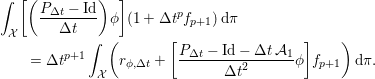 $$\begin{eqnarray}\displaystyle & & \displaystyle \int _{{\mathcal{X}}}\biggl[\biggl(\displaystyle \frac{P_{{\rm\Delta}t}-\text{Id}}{{\rm\Delta}t}\biggr){\it\phi}\biggr](1+{\rm\Delta}t^{p}f_{p+1})\,\text{d}{\it\pi}\nonumber\\ \displaystyle & & \displaystyle \qquad ={\rm\Delta}t^{p+1}\int _{{\mathcal{X}}}\biggl(r_{{\it\phi},{\rm\Delta}t}+\biggl[\frac{P_{{\rm\Delta}t}-\text{Id}-{\rm\Delta}t\,{\mathcal{A}}_{1}}{{\rm\Delta}t^{2}}{\it\phi}\biggr]f_{p+1}\biggr)\,\text{d}{\it\pi}.\end{eqnarray}$$
so that (3.18) holds for  ${\it\varphi}=(\text{Id}-P_{{\rm\Delta}t}){\it\phi}/{\rm\Delta}t$.
The second step of the proof is to extend (3.18) to all functions in  ${\mathcal{S}}_{0}$. Of course, we would like to replace
 ${\it\phi}$ with
 ${\rm\Delta}t(\text{Id}-P_{{\rm\Delta}t})^{-1}{\it\varphi}$ in the previous estimates. However, there are two
obstructions to this approach: (i) the inverse
 ${\rm\Delta}t(\text{Id}-P_{{\rm\Delta}t})^{-1}$ is well defined only on spaces of functions with
average 0 with respect to
 ${\it\pi}_{{\rm\Delta}t}$, and (ii), when this is the case, we typically do not have
any control on the derivatives of
 ${\rm\Delta}t(\text{Id}-P_{{\rm\Delta}t})^{-1}{\it\varphi}$, but only on the function itself (by results such as
Corollary 2.26). Our strategy is to construct an operator
 $Q_{{\rm\Delta}t}$ which leaves
 ${\mathcal{S}}_{0}$ invariant and is an approximate inverse of
 $(\text{Id}-P_{{\rm\Delta}t})/{\rm\Delta}t$ on
 ${\mathcal{S}}_{0}$. Since
 $(\text{Id}-P_{{\rm\Delta}t}){\it\varphi}/{\rm\Delta}t={\mathcal{A}}_{1}{\it\varphi}+\text{O}({\rm\Delta}t)$, we expect the inverse operator to be
 ${\mathcal{A}}_{1}^{-1}$ at dominant order in
 ${\rm\Delta}t$.
The first task is to restrict  $\text{Id}-P_{{\rm\Delta}t}$ to
 ${\mathcal{S}}_{0}$ via
 ${\rm\Pi}(\text{Id}-P_{{\rm\Delta}t}){\rm\Pi}$, using the projection operator
 ${\rm\Pi}$ defined in (3.3). Then (3.21)
implies
 $$\begin{eqnarray}\int _{{\mathcal{X}}}\biggl[{\rm\Pi}\biggl(\displaystyle \frac{P_{{\rm\Delta}t}-\text{Id}}{{\rm\Delta}t}\biggr){\rm\Pi}{\it\phi}\biggr]\,\text{d}{\it\pi}_{{\rm\Delta}t}=-\frac{1}{{\rm\Delta}t}\int _{{\mathcal{X}}}(P_{{\rm\Delta}t}{\it\phi})\,\text{d}{\it\pi},\end{eqnarray}$$
for  ${\it\phi}\in {\mathcal{S}}_{0}$ (so that
 ${\rm\Pi}{\it\phi}={\it\phi}$). Further, using the fact that
 $f_{p+1}$ is of average 0 with respect to
 ${\it\pi}$, (3.22)
leads to
 $$\begin{eqnarray}\displaystyle & & \displaystyle \int _{{\mathcal{X}}}\biggl[{\rm\Pi}\biggl(\displaystyle \frac{P_{{\rm\Delta}t}-\text{Id}}{{\rm\Delta}t}\biggr){\rm\Pi}{\it\phi}\biggr](1+{\rm\Delta}t^{p}f_{p+1})\,\text{d}{\it\pi}=-\frac{1}{{\rm\Delta}t}\int _{{\mathcal{X}}}(P_{{\rm\Delta}t}{\it\phi})\,\text{d}{\it\pi}\nonumber\\ \displaystyle & & \displaystyle \qquad +{\rm\Delta}t^{p+1}\int _{{\mathcal{X}}}\biggl(r_{{\it\phi},{\rm\Delta}t}+\biggl[\frac{P_{{\rm\Delta}t}-\text{Id}-{\rm\Delta}t\,{\mathcal{A}}_{1}}{{\rm\Delta}t^{2}}{\it\phi}\biggr]f_{p+1}\biggr)\,\text{d}{\it\pi}.\end{eqnarray}$$
This shows that, for any  ${\it\phi}\in {\mathcal{S}}_{0}$,
 $$\begin{eqnarray}\displaystyle & & \displaystyle \int _{{\mathcal{X}}}\biggl[{\rm\Pi}\biggl(\displaystyle \frac{P_{{\rm\Delta}t}-\text{Id}}{{\rm\Delta}t}\biggr){\rm\Pi}{\it\phi}\biggr]\,\text{d}{\it\pi}_{{\rm\Delta}t}=\int _{{\mathcal{X}}}\biggl[{\rm\Pi}\biggl(\displaystyle \frac{P_{{\rm\Delta}t}-\text{Id}}{{\rm\Delta}t}\biggr){\rm\Pi}{\it\phi}\biggr](1+{\rm\Delta}t^{p}f_{p+1})\,\text{d}{\it\pi}\nonumber\\ \displaystyle & & \displaystyle \qquad -\,{\rm\Delta}t^{p+1}\int _{{\mathcal{X}}}\biggl(r_{{\it\phi},{\rm\Delta}t}+\biggl[\frac{P_{{\rm\Delta}t}-\text{Id}-{\rm\Delta}t\,{\mathcal{A}}_{1}}{{\rm\Delta}t^{2}}{\it\phi}\biggr]f_{p+1}\biggr)\,\text{d}{\it\pi}.\nonumber\end{eqnarray}$$
We next consider an approximate inverse operator  $Q_{{\rm\Delta}t}$ which leaves
 ${\mathcal{S}}_{0}$ invariant, and is such that
 $$\begin{eqnarray}{\rm\Pi}\biggl(\frac{P_{{\rm\Delta}t}-\text{Id}}{{\rm\Delta}t}\biggr){\rm\Pi}Q_{{\rm\Delta}t}{\it\varphi}={\it\varphi}+{\rm\Delta}t^{p+1}\widetilde{r}_{{\it\varphi},{\rm\Delta}t},\quad \text{for all }{\it\varphi}\in {\mathcal{S}}_{0},\end{eqnarray}$$
with  $\Vert \widetilde{r}_{{\it\varphi},{\rm\Delta}t}\Vert _{L_{{\mathcal{K}}_{m}}^{\infty }}$ uniformly bounded with respect to
 ${\rm\Delta}t$ for some integer
 $m$. Such operators are constructed as follows. The
fundamental idea is to truncate the formal series expansion of the inverse
of the operator
 $A+{\rm\Delta}t\,B=A(\text{Id}+{\rm\Delta}t\,A^{-1}B)$ in powers of
 $A^{-1}B$:
 $$\begin{eqnarray}A^{-1}-{\rm\Delta}t\,A^{-1}BA^{-1}+{\rm\Delta}t^{2}\,A^{-1}BA^{-1}BA^{-1}+\cdots \,.\end{eqnarray}$$
In the present situation, we set  $A={\rm\Pi}{\mathcal{A}}_{1}{\rm\Pi}$ and
 $B={\rm\Pi}{\mathcal{A}}_{2}{\rm\Pi}+\cdots +{\rm\Delta}t^{p-1}{\rm\Pi}{\mathcal{A}}_{p+1}{\rm\Pi}$. Note that perturbative arguments cannot be used to make
sense of the formal infinite series since
 $B$ usually involves differential operators of higher order than
 $A$, so that
 $B$ cannot be controlled by
 $A$ (in contrast to the situation we will encounter later on
in Theorem 5.2).
Introducing
 $\widetilde{{\mathcal{A}}}_{k}={\rm\Pi}{\mathcal{A}}_{k}{\rm\Pi}$ for notational simplicity, we consider
 $$\begin{eqnarray}\widetilde{Q}_{{\rm\Delta}t}=\widetilde{{\mathcal{A}}}_{1}^{-1}\mathop{\sum }_{n=0}^{p}(-1)^{n}{\rm\Delta}t^{n}\,(B\widetilde{{\mathcal{A}}}_{1}^{-1})^{n}.\end{eqnarray}$$
We next remove operators with powers of  ${\rm\Delta}t$ larger than or equal to
 $p+1$ (arising from the higher-order terms in the expression of
 $B\widetilde{{\mathcal{A}}}_{1}^{-1}$) in order to write down an expression for
 $Q_{{\rm\Delta}t}$ involving only powers of
 ${\rm\Delta}t$ smaller than or equal to
 $p$. Finally, the so-constructed operator,
 $$\begin{eqnarray}\displaystyle Q_{{\rm\Delta}t} & = & \displaystyle \widetilde{{\mathcal{A}}}_{1}^{-1}-{\rm\Delta}t\widetilde{{\mathcal{A}}}_{1}^{-1}\widetilde{{\mathcal{A}}}_{2}\widetilde{{\mathcal{A}}}_{1}^{-1}+{\rm\Delta}t^{2}(\widetilde{{\mathcal{A}}}_{1}^{-1}\widetilde{{\mathcal{A}}}_{2}\widetilde{{\mathcal{A}}}_{1}^{-1}\widetilde{{\mathcal{A}}}_{2}\widetilde{{\mathcal{A}}}_{1}^{-1}-\widetilde{{\mathcal{A}}}_{1}^{-1}\widetilde{{\mathcal{A}}}_{3}\widetilde{{\mathcal{A}}}_{1}^{-1})\nonumber\\ \displaystyle & & \displaystyle \quad +{\rm\Delta}t^{3}{\mathcal{Q}}_{3}+\cdots +{\rm\Delta}t^{p}{\mathcal{Q}}_{p},\nonumber\end{eqnarray}$$
is a well defined operator which leaves  ${\mathcal{S}}_{0}$ invariant (since its action is given by the application of
at most
 $p$ operations of the form
 $\widetilde{{\mathcal{A}}}_{k}\widetilde{{\mathcal{A}}}_{1}^{-1}$, and a final application of
 $\widetilde{{\mathcal{A}}}_{1}^{-1}$) and is such that (3.25) holds true.
In order to conclude, it remains to replace  ${\it\phi}$ with
 $Q_{{\rm\Delta}t}{\it\varphi}$, and gather all the higher-order terms in
 $R_{{\it\varphi},{\rm\Delta}t}$. This gives the desired equality (3.18) for functions in
 ${\mathcal{S}}_{0}$.
We next illustrate the strategy presented here applied to overdamped Langevin and Langevin dynamics. We postpone numerical illustration of the results of Theorem 3.3 to Figure 5.1 in Section 5.3. Indeed, as explained in Section 3.3.4, the leading-order correction term can be computed as some integrated correlation function, for which we provide elements of numerical analysis later on, in Section 5.3.
3.3.2 Application to overdamped Langevin dynamics
For overdamped Langevin dynamics, we consider for simplicity the case of a simple
Euler–Maruyama discretization of a dynamics defined on the compact
position space  ${\mathcal{D}}=(L\mathbb{T})^{d}$:
 $$\begin{eqnarray}q^{n+1}=q^{n}-{\rm\Delta}t\,{\rm\nabla}V(q^{n})+\sqrt{\frac{2{\rm\Delta}t}{{\it\beta}}}\,G^{n}.\end{eqnarray}$$
The results below can be easily generalized to other discretization schemes. On the other hand, an extension to unbounded position spaces is not trivial (see Kopec Reference Kopec2015), although several results can be stated in a weaker form than the results given below.
The first task is to find an expansion of the transition operator  $P_{{\rm\Delta}t}$ defined in (3.9) in powers of
 ${\rm\Delta}t$: see (3.15). Simple but lengthy computations show that (see
Section 4.9.2 in Leimkuhler et al. Reference Leimkuhler, Matthews and Stoltz2015)
 $$\begin{eqnarray}P_{{\rm\Delta}t}{\it\varphi}={\it\varphi}+{\rm\Delta}t\,{\mathcal{L}}{\it\varphi}+{\rm\Delta}t^{2}{\mathcal{A}}_{2}{\it\varphi}+{\rm\Delta}t^{3}r_{{\it\varphi},{\rm\Delta}t},\end{eqnarray}$$
where  $\Vert r_{{\it\varphi},{\rm\Delta}t}\Vert _{L^{\infty }}\leqslant K$ for
 ${\rm\Delta}t$ sufficiently small and
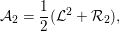 $$\begin{eqnarray}{\mathcal{A}}_{2}=\frac{1}{2}({\mathcal{L}}^{2}+{\mathcal{R}}_{2}),\end{eqnarray}$$
with
 $$\begin{eqnarray}{\mathcal{R}}_{2}{\it\varphi}=\frac{2}{{\it\beta}}{\rm\nabla}^{2}V:{\rm\nabla}^{2}{\it\varphi}+\frac{1}{{\it\beta}}{\rm\nabla}({\rm\Delta}V)\cdot {\rm\nabla}{\it\varphi}-{\rm\nabla}V^{T}({\rm\nabla}^{2}V){\rm\nabla}{\it\varphi}.\end{eqnarray}$$
We want to apply Theorem 3.3 with  $p=1$. In summary, there are three types of assumptions to be
checked:
(i) assumptions on the generator
${\mathcal{L}}={\mathcal{A}}_{1}$ of the continuous dynamics;(ii) assumptions on the operator
${\mathcal{A}}_{2}$, whose action is given by (3.28);(iii) assumptions on the invariant measure of the numerical scheme.


First, recall that, as discussed after Definition 3.1,  ${\mathcal{K}}_{n}(q)=\mathbf{1}$ for all
 $n\geqslant 0$ when
 ${\mathcal{D}}$ is bounded, so that
 ${\mathcal{S}}=C^{\infty }({\mathcal{D}})$. Standard results of elliptic regularity then show that
 ${\mathcal{L}}^{-1}$ is a well-defined operator from
 $$\begin{eqnarray}{\mathcal{S}}_{0}=\biggl\{f\in C^{\infty }({\mathcal{D}})\,\bigg|\,\int _{{\mathcal{D}}}f\,\text{d}{\it\nu}=0\biggr\}\end{eqnarray}$$
to itself. For dynamics in the full space  ${\mathcal{D}}=\mathbb{R}^{d}$, additional assumptions on the potential are needed to obtain
the stability of
 ${\mathcal{S}}$ with the choice
 ${\mathcal{K}}_{n}(q)=1+|q|^{n}$, and the proof of this stability result is much more involved
(see Kopec Reference Kopec2015).
It can now be easily checked that  $g_{2}$ is well defined and belongs to
 ${\mathcal{S}}$ (recall that, as discussed after Theorem 3.3, it automatically has
average 0 with respect to
 ${\it\pi}$). To obtain the precise expression for
 $g_{2}$, we use integration by parts to compute
 $$\begin{eqnarray}\displaystyle \int _{{\mathcal{D}}}{\mathcal{R}}_{2}{\it\varphi}\,\text{d}{\it\nu} & = & \displaystyle -\frac{1}{{\it\beta}}\int _{{\mathcal{D}}}{\rm\nabla}\biggl({\rm\Delta}V-\frac{{\it\beta}}{2}|{\rm\nabla}V|^{2}\biggr)\cdot {\rm\nabla}{\it\varphi}\,\text{d}{\it\nu}\nonumber\\ \displaystyle & = & \displaystyle \int _{{\mathcal{D}}}{\mathcal{L}}\biggl({\rm\Delta}V-\frac{{\it\beta}}{2}|{\rm\nabla}V|^{2}\biggr){\it\varphi}\,\text{d}{\it\nu}.\nonumber\end{eqnarray}$$
Using that, for all  ${\it\varphi}\in {\mathcal{S}}$,
 $$\begin{eqnarray}\int _{{\mathcal{D}}}{\mathcal{A}}_{2}{\it\varphi}\,\text{d}{\it\nu}=\frac{1}{2}\int _{{\mathcal{D}}}{\mathcal{R}}_{2}{\it\varphi}\,\text{d}{\it\nu}=\int _{{\mathcal{D}}}g_{2}{\it\varphi}\,\text{d}{\it\nu},\end{eqnarray}$$
one obtains
 $$\begin{eqnarray}g_{2}=\frac{1}{2}{\mathcal{L}}\biggl({\rm\Delta}V-\frac{{\it\beta}}{2}|{\rm\nabla}V|^{2}\biggr).\end{eqnarray}$$
Since  ${\mathcal{A}}_{1}={\mathcal{L}}={\mathcal{L}}^{\ast }$ on
 $L^{2}({\it\nu})$, we in fact obtain the analytical expression of the correction function
 $f_{2}$ defined in (3.19):
 $$\begin{eqnarray}f_{2}=-\frac{1}{2}\biggl({\rm\Delta}V-\frac{{\it\beta}}{2}|{\rm\nabla}V|^{2}-\frac{a_{{\it\beta},V}}{2}\biggr),\end{eqnarray}$$
where
 $$\begin{eqnarray}a_{{\it\beta},V}=\int _{{\mathcal{D}}}{\rm\Delta}V\,\text{d}{\it\nu}={\it\beta}\int _{{\mathcal{D}}}|{\rm\nabla}V|^{2}\,\text{d}{\it\nu}\end{eqnarray}$$
is a constant ensuring that  $f_{2}$ is of average 0 with respect to
 ${\it\nu}$.
Finally, to prove that an invariant measure  ${\it\pi}_{{\rm\Delta}t}$ exists for the numerical scheme, we rely on
Theorem 2.25. The
Lyapunov condition of Assumption 2.23 is trivially satisfied since the position space is
compact. Therefore, the only property to prove is the minorization condition of
Assumption 2.24.
Since the space is bounded, it readily follows from (3.26) that, for any Borel subset
 $S\subset {\mathcal{D}}$,
 $$\begin{eqnarray}\displaystyle \mathbb{P}(q^{1}\in S|q^{0}=q) & {\geqslant} & \displaystyle \mathbb{P}\biggl(\sqrt{\frac{2{\rm\Delta}t}{{\it\beta}}}G^{1}\in S-q+{\rm\Delta}t{\rm\nabla}V(q)\biggr)\nonumber\\ \displaystyle & {\geqslant} & \displaystyle \inf _{|{\mathcal{Q}}|\leqslant |{\mathcal{D}}|+\Vert {\rm\nabla}V\Vert _{L^{\infty }}}\mathbb{P}\biggl(\sqrt{\frac{2{\rm\Delta}t}{{\it\beta}}}G^{1}\in S-{\mathcal{Q}}\biggr)\nonumber\\ \displaystyle & = & \displaystyle \biggl(\frac{{\it\beta}}{4{\it\pi}{\rm\Delta}t}\biggr)^{d/2}\inf _{|{\mathcal{Q}}|\leqslant |{\mathcal{D}}|+\Vert {\rm\nabla}V\Vert _{L^{\infty }}}\int _{S-{\mathcal{Q}}}\exp \biggl(-\frac{{\it\beta}|g|^{2}}{4{\rm\Delta}t}\biggr)\,\text{d}g,\nonumber\end{eqnarray}$$
where the first inequality is due to the fact that the
contributions associated with periodic images of  $q$ are not taken into account. The minorization condition then
follows by defining the measure
 $$\begin{eqnarray}\widetilde{{\it\lambda}}_{{\rm\Delta}t}(S)=\inf _{|{\mathcal{Q}}|\leqslant |{\mathcal{D}}|+\Vert {\rm\nabla}V\Vert _{L^{\infty }}}\int _{S-{\mathcal{Q}}}\exp \biggl(-\frac{{\it\beta}|g|^{2}}{4{\rm\Delta}t}\biggr)\,\text{d}g,\end{eqnarray}$$
normalizing it as  ${\it\lambda}_{{\rm\Delta}t}(S)=\widetilde{{\it\lambda}}_{{\rm\Delta}t}(S)/\widetilde{{\it\lambda}}_{{\rm\Delta}t}({\mathcal{D}})$, and introducing
 $$\begin{eqnarray}{\it\eta}_{{\rm\Delta}t}=(4{\it\pi}{\rm\Delta}t/{\it\beta})^{-d/2}\widetilde{{\it\lambda}}_{{\rm\Delta}t}({\mathcal{D}}).\end{eqnarray}$$
We state below a minorization condition stronger than is needed for
Assumption 2.24, but
which will prove useful later on in Section 5.3. We call it a ‘uniform minorization
condition’ since, in contrast to the above computations, the lower
bound  ${\it\eta}$ and the probability measure
 ${\it\lambda}$ do not depend on the time step
 ${\rm\Delta}t$ provided it is sufficiently small. To obtain such a condition,
we have to consider evolutions over fixed physical times
 $T\simeq n{\rm\Delta}t>0$, which amounts to iterating the elementary evolution
 $P_{{\rm\Delta}t}$ over
 $\lceil T/{\rm\Delta}t\rceil$ time steps (where
 $\lceil x\rceil$ denotes the smallest integer larger than
 $x$).
Lemma 3.4 (uniform minorization condition).
Consider the evolution operator  $P_{{\rm\Delta}t}$ associated with the Euler–Maruyama
discretization (3.26) on
the position space
 ${\mathcal{D}}=(L\mathbb{T})^{d}$, and a given integration time
 $T>0$. There exist
 ${\rm\Delta}t^{\ast },{\it\eta}>0$ and a probability measure
 ${\it\lambda}$ such that, for any bounded, measurable non-negative
function
 $f$, for any
 ${\rm\Delta}t\in (0,{\rm\Delta}t^{\ast }]$ and for any
 $q\in {\mathcal{D}}$,
 $$\begin{eqnarray}(P_{{\rm\Delta}t}^{\lceil T/{\rm\Delta}t\rceil }f)(q)\geqslant {\it\eta}\int _{{\mathcal{D}}}f\,\text{d}{\it\lambda}.\end{eqnarray}$$
Such estimates were obtained in Bou-Rabee and Hairer (Reference Bou-Rabee and Hairer2013) in unbounded spaces  ${\mathcal{D}}$ for a class of Metropolis–Hastings schemes whose
proposition kernel is (3.26).
See also Fathi, Homman and Stoltz (Reference Fathi, Homman and Stoltz2014)
and Fathi and Stoltz (Reference Fathi and Stoltz2015) for related
results on bounded spaces, as well as Leimkuhler
et al. (Reference Leimkuhler, Matthews and Stoltz2015)
and Redon, Stoltz and Trstanova (Reference Redon, Stoltz and Trstanova2016) for
discretizations of Langevin dynamics.
Proof. It is sufficient to prove the result for indicator functions of Borel sets  $S\subset {\mathcal{D}}$. We therefore aim to prove that
 $$\begin{eqnarray}\mathbb{P}(q^{\lceil T/{\rm\Delta}t\rceil }\in S\mid q^{0}=q)\geqslant {\it\eta}\,{\it\lambda}(S),\end{eqnarray}$$
for a probability measure  ${\it\lambda}$ and a constant
 ${\it\eta}>0$. The idea of the proof is to explicitly rewrite
 $q^{n}$ as a perturbation of the reference evolution corresponding
to
 ${\rm\nabla}V=0$. Since we consider
 $C^{\infty }$ potentials and the position space is compact,
the perturbation can be uniformly controlled. More precisely, an immediate
induction argument based on (3.26) gives
 $$\begin{eqnarray}q^{n}=q^{0}+{\mathcal{G}}^{n}+{\mathcal{F}}^{n},\end{eqnarray}$$
with
 $$\begin{eqnarray}{\mathcal{G}}^{n}=\sqrt{\frac{2{\rm\Delta}t}{{\it\beta}}}\mathop{\sum }_{k=0}^{n-1}G^{k},\quad {\mathcal{F}}^{n}=-{\rm\Delta}t\mathop{\sum }_{k=0}^{n-1}{\rm\nabla}V(q^{k}).\end{eqnarray}$$
Let us now fix  $n=\lceil T/{\rm\Delta}t\rceil$ (so that
 $T\leqslant n{\rm\Delta}t\leqslant T+{\rm\Delta}t$). Then
 $|{\mathcal{F}}^{n}|\leqslant \Vert {\rm\nabla}V\Vert _{L^{\infty }}(T+{\rm\Delta}t)$, while
 ${\mathcal{G}}^{n}$ is a Gaussian random variable with covariance matrix
 $2n{\rm\Delta}t{\it\beta}^{-1}\,\text{Id}_{d}$. Therefore,
 $$\begin{eqnarray}\displaystyle \mathbb{P}(q^{n}\in S\mid q^{0}=q) & {\geqslant} & \displaystyle \mathbb{P}({\mathcal{G}}^{n}\in S-q-{\mathcal{F}}^{n})\nonumber\\ \displaystyle & = & \displaystyle \biggl(\displaystyle \frac{{\it\beta}}{2{\it\pi}n{\rm\Delta}t}\biggr)^{d/2}\int _{S-q-{\mathcal{F}}^{n}}\exp \biggl(-\frac{{\it\beta}|g|^{2}}{2n{\rm\Delta}t}\biggr)\,\text{d}g.\nonumber\end{eqnarray}$$
In the latter expression and below, we assume that the
random variable  ${\mathcal{G}}^{n}$ has values in
 $\mathbb{R}^{d}$ rather than
 ${\mathcal{D}}$, and regard
 $S-q-{\mathcal{F}}^{n}$ as a subset of
 $\mathbb{R}^{d}$ rather than
 ${\mathcal{D}}$. This amounts to neglecting the periodic images, and
henceforth reduces the probability on the right-hand side of the above
inequality. This is not a problem, however, since we seek a lower bound.
Now, for
 ${\rm\Delta}t$ sufficiently small, we have
 $T/2\leqslant n{\rm\Delta}t\leqslant 2T$, so
 $$\begin{eqnarray}\biggl(\displaystyle \frac{1}{n{\rm\Delta}t}\biggr)^{d/2}\!\!\int _{S-q-{\mathcal{F}}^{n}}\!\exp \biggl(-\frac{{\it\beta}|g|^{2}}{2n{\rm\Delta}t}\biggr)\,\text{d}g\geqslant \biggl(\displaystyle \frac{1}{2T}\biggr)^{d/2}\!\!\int _{S-q-{\mathcal{F}}^{n}}\!\exp \biggl(-\frac{{\it\beta}|g|^{2}}{T}\biggr)\,\text{d}g.\end{eqnarray}$$
Since the state space is compact, there exists  $R>0$ such that
 $|q+{\mathcal{F}}^{n}|\leqslant R$ for any
 $q\in {\mathcal{D}}$. The conclusion then easily follows by defining the
probability measure
 ${\it\lambda}$ as
 $$\begin{eqnarray}{\it\lambda}(S)=Z_{R}^{-1}\inf _{|Q|\leqslant R}\int _{S+Q}\exp \biggl(-\frac{{\it\beta}|g|^{2}}{T}\biggr)\,\text{d}g,\end{eqnarray}$$
for all  $S\subset {\mathcal{D}}$, and setting
 ${\it\eta}=Z_{R}(4{\it\pi}T/{\it\beta})^{-d/2}$.
The proof of Lemma 3.4
shows that the measure  ${\it\lambda}$ has a positive density with respect to the Lebesgue measure.
Application of Theorem 2.25, together with an argument similar to that used to obtain (2.78) from the decay at multiples of
a given time, gives the following exponential convergence.
Corollary 3.5 (ergodicity of Euler–Maruyama for compact spaces).
There exists  ${\rm\Delta}t^{\ast }>0$ such that, for any
 ${\rm\Delta}t\in (0,{\rm\Delta}t^{\ast }]$, the Markov chain associated with
 $P_{{\rm\Delta}t}$ has a unique invariant probability measure
 ${\it\nu}_{{\rm\Delta}t}$. This measure admits a density with respect to the
Lebesgue measure. Moreover, there exist
 $C,{\it\kappa}>0$ such that, for all functions
 $f\in L^{\infty }({\mathcal{D}})$,
 $$\begin{eqnarray}\biggl\|P_{{\rm\Delta}t}^{n}f-\int _{{\mathcal{D}}}f\,\text{d}{\it\nu}_{{\rm\Delta}t}\biggr\|_{L^{\infty }}\leqslant C\,\text{e}^{-{\it\kappa}n{\rm\Delta}t}\,\Vert f\Vert _{L^{\infty }},\quad \text{for all }n\in \mathbb{N}.\end{eqnarray}$$
The fact that  ${\it\nu}_{{\rm\Delta}t}$ admits a density with respect to Lebesgue measure
 $\text{d}q$ follows from the minorization condition stated in
Lemma 3.4, which
ensures that the Markov chain is irreducible with respect to Lebesgue measure.
3.3.3 Application to Langevin dynamics
Many numerical schemes have been proposed for Langevin dynamics. The first ones, such as the BBK scheme proposed in Brünger, Brooks and Karplus (Reference Brünger, Brooks and Karplus1984), were often obtained by modifications of numerical schemes for deterministic Hamiltonian dynamics. Various other schemes have been proposed since then; see for instance Skeel and Izaguirre (Reference Skeel and Izaguirre2002), Melchionna (Reference Melchionna2007), Bussi and Parrinello (Reference Bussi and Parrinello2007), Thalmann and Farago (Reference Thalmann and Farago2007) and Leimkuhler and Matthews (Reference Leimkuhler and Matthews2013a) for recent suggestions.
One systematic way to derive numerical schemes of arbitrary order is to resort to splitting schemes to analytically integrate the various parts of the dynamics. However, proving rigorous ergodicity results on the corresponding numerical schemes has so far been done only for compact position spaces (see Leimkuhler et al. Reference Leimkuhler, Matthews and Stoltz2015). For unbounded position spaces, implicit schemes should be considered (see Mattingly et al. Reference Mattingly, Stuart and Higham2002, Kopec Reference Kopec2015), in which case some geometric convergence can be achieved. Alternatively, it is always possible to superimpose a Metropolis–Hastings step upon the discretization under consideration in order to stabilize the numerical method and ensure the existence of an invariant measure.
We restrict ourselves in the rest of this section to compact position spaces  ${\mathcal{D}}=(L\mathbb{T})^{d}$. Let us first decompose the generator of Langevin dynamics as
 ${\mathcal{L}}=A+B+{\it\gamma}C$, with
 $$\begin{eqnarray}A=M^{-1}p\cdot {\rm\nabla}_{q},\quad B=-{\rm\nabla}V(q)\cdot {\rm\nabla}_{p},\quad C=-M^{-1}p\cdot {\rm\nabla}_{p}+\frac{1}{{\it\beta}}{\rm\Delta}_{p}.\end{eqnarray}$$
First-order splitting schemes are obtained via a
Lie–Trotter splitting of the elementary evolutions generated by  $A,B,{\it\gamma}C$. There are six possible schemes of the general form
 $$\begin{eqnarray}P_{{\rm\Delta}t}^{Z,Y,X}=\text{e}^{{\rm\Delta}tZ}\,\text{e}^{{\rm\Delta}tY}\,\text{e}^{{\rm\Delta}tX},\end{eqnarray}$$
with all possible permutations  $(Z,Y,X)$ of
 $(A,B,{\it\gamma}C)$. For instance, the numerical scheme associated with
 $P_{{\rm\Delta}t}^{B,A,{\it\gamma}C}$ is
 $$\begin{eqnarray}\displaystyle \widetilde{p}^{n+1} & = & \displaystyle p^{n}-{\rm\Delta}t\,{\rm\nabla}V(q^{n}),\end{eqnarray}$$
 $$\begin{eqnarray}\displaystyle q^{n+1} & = & \displaystyle q^{n}+{\rm\Delta}t\,M^{-1}\widetilde{p}^{n+1},\end{eqnarray}$$
 $$\begin{eqnarray}\displaystyle p^{n+1} & = & \displaystyle {\it\alpha}_{{\rm\Delta}t}\widetilde{p}^{n+1}+\sqrt{\frac{1-{\it\alpha}_{{\rm\Delta}t}^{2}}{{\it\beta}}M}\,G^{n},\end{eqnarray}$$
 ${\it\alpha}_{{\rm\Delta}t}=\exp (-{\it\gamma}M^{-1}{\rm\Delta}t)$, and
 $(G^{n})_{n\geqslant 0}$ are i.i.d. Gaussian random vectors with identity
covariance. Second-order splitting schemes are obtained by a Strang splitting of
the elementary evolutions generated by
 $A,B,{\it\gamma}C$. There are again six possible schemes, which are of the general
form
 $$\begin{eqnarray}P_{{\rm\Delta}t}^{Z,Y,X,Y,Z}=\text{e}^{{\rm\Delta}tZ/2}\,\text{e}^{{\rm\Delta}tY/2}\,\text{e}^{{\rm\Delta}tX}\,\text{e}^{{\rm\Delta}tY/2}\,\text{e}^{{\rm\Delta}tZ/2},\end{eqnarray}$$
with the same possible orderings as for first-order schemes. In fact, as already proved in Bou-Rabee and Owhadi (Reference Bou-Rabee and Owhadi2010), second-order accuracy on the invariant measure can be obtained by resorting to a first-order splitting between the Hamiltonian and the Ornstein–Uhlenbeck parts, and discretizing the Hamiltonian part with a second-order scheme. This corresponds to evolution operators of so-called geometric Langevin algorithm type, such as
 $$\begin{eqnarray}P_{{\rm\Delta}t}^{B,A,B,{\it\gamma}C}=\text{e}^{{\rm\Delta}tB/2}\,\text{e}^{{\rm\Delta}tA}\,\text{e}^{{\rm\Delta}tB/2}\,\text{e}^{{\it\gamma}{\rm\Delta}tC}.\end{eqnarray}$$
The latter scheme amounts to first performing one iteration of the
Verlet scheme ( $\text{e}^{{\rm\Delta}tB/2}\,\text{e}^{{\rm\Delta}tA}\,\text{e}^{{\rm\Delta}tB/2}$) and then updating the momenta via an analytic integration of
the Ornstein–Uhlenbeck process (which corresponds to
 $\text{e}^{{\it\gamma}{\rm\Delta}tC}$). Among all these splitting schemes, some lead to smaller errors
on the invariant measure. Moreover, only certain geometric Langevin algorithms and
second-order splitting schemes admit invariant measures consistent with
 ${\it\nu}$ in the overdamped regime
 ${\it\gamma}\rightarrow 0$. See Leimkuhler et al. (Reference Leimkuhler, Matthews and Stoltz2015) for more precise statements.
Remark 3.6 (stability).
Stability is a necessary condition for the existence of an invariant measure  ${\it\mu}_{{\rm\Delta}t}$ for the numerical scheme under consideration. This
property is guaranteed by the existence of a Lyapunov function
 ${\mathcal{K}}$ for the transition operator
 $P_{{\rm\Delta}t}$ (see Theorem 2.25), which typically requires the time step
 ${\rm\Delta}t$ to be sufficiently small. For discretizations of Langevin
dynamics, the stability conditions are similar to those obtained for
discretizations of the Hamiltonian dynamics, which correspond to
 ${\it\gamma}=0$; see Leimkuhler and Matthews (Reference Leimkuhler and Matthews2013b, Reference Leimkuhler and Matthews2015). Note indeed that all the
splitting schemes introduced above reduce to a symplectic discretization of
the Hamiltonian dynamics when
 ${\it\gamma}=0$. Recall also that the numerical stability of these schemes
requires the time step
 ${\rm\Delta}t$ to be sufficiently small. For one-dimensional systems with
a harmonic potential
 $V(q)={\it\omega}^{2}q^{2}/2$, the stability constraint reads
 ${\it\omega}{\rm\Delta}t<2$. For more general systems, this means that the time step
has to be of the order of a fraction of the period of the fastest
vibrational modes.
As for overdamped Langevin dynamics, Theorem 3.3 can be used to obtain error estimates on the invariant
measure (i.e. (3.18) with  ${\it\pi}$ replaced by
 ${\it\mu}$), with either
 $p=1$ for first-order splitting schemes or
 $p=2$ for second-order splitting schemes and geometric Langevin
algorithms. We consider the hierarchy of scale functions
 ${\mathcal{K}}_{n}(q,p)=1+|p|^{2n}$. There are three types of assumptions to be checked.
(i) Assumptions on the generator
${\mathcal{A}}_{1}={\mathcal{L}}$ of the continuous dynamics.
The stability of the space of smooth functions ${\mathcal{S}}_{0}$ under ${\mathcal{L}}^{-1}$ follows from careful analysis of the proof presented in
Talay (Reference Talay2002), as provided in
Kopec (Reference Kopec2015,
Appendix A) for unbounded position spaces (the adaptation to
compact position spaces allowing simplification of some arguments).(ii) Assumptions on the invariant measure
${\it\mu}_{{\rm\Delta}t}$ of the numerical scheme. It
can be proved that there exists an invariant measure ${\it\mu}_{{\rm\Delta}t}$ such that ${\mathcal{K}}_{n}\in L^{1}({\it\mu}_{{\rm\Delta}t})$ for all $n\geqslant 0$. In fact, similarly to Corollary 3.5, a much stronger result
can be stated, namely the exponential convergence of the law to a unique
invariant measure, in any space $L_{{\mathcal{K}}_{n}}^{\infty }({\mathcal{E}})$ and with a rate independent of the time step (see
Leimkuhler et al. Reference Leimkuhler, Matthews and Stoltz2015). The proof of the existence
and uniqueness of the invariant measure can be somewhat simplified if no
uniform convergence rate is sought (as done in Mattingly
et al. Reference Mattingly, Stuart and Higham2002).(iii) Assumptions on the differential operators arising in the expansion in powers of
${\rm\Delta}t$ of the evolution operator $P_{{\rm\Delta}t}$. The expressions of these operators are conveniently
obtained for splitting schemes with the
Baker–Campbell–Hausdorff formula; see for instance
the presentation in Hairer et al. (Reference Hairer, Lubich and Wanner2006, Section III.4.2).
Such computations are reported in Leimkuhler and Matthews (Reference Leimkuhler and Matthews2013a) and
Leimkuhler et al. (Reference Leimkuhler, Matthews and Stoltz2015).


3.3.4 Removing the systematic error
The estimate (3.18) not only allows us to estimate the order of magnitude of the error on average properties arising from the discretization of the dynamics, but also provides an expression of the leading-order term in the difference as
 $$\begin{eqnarray}\int _{{\mathcal{X}}}{\it\varphi}\,\text{d}{\it\pi}_{{\rm\Delta}t}-\int _{{\mathcal{X}}}{\it\varphi}\,\text{d}{\it\pi}={\rm\Delta}t^{p}\int _{{\mathcal{X}}}{\it\varphi}f_{p+1}\,\text{d}{\it\pi}+\text{O}({\rm\Delta}t^{p+1}).\end{eqnarray}$$
There are two principal strategies for reducing/removing the leading-order term on the right-hand side of the above equality.
(1) Using Romberg extrapolation as already suggested in Talay and Tubaro (Reference Talay and Tubaro1990), by performing simulations with two different time steps, in order to eliminate the leading-order error term by an appropriate linear combination of the associated estimators.
(2) Directly estimating the correction term by reformulating it as an integrated correlation function. This is possible when
${\mathcal{A}}_{1}={\mathcal{L}}$, namely for schemes of weak order at least one. Indeed,
the expression (3.19) for $f_{p+1}$ leads to (3.32)where we have implicitly assumed that decay estimates hold for the semigroup$$\begin{eqnarray}\displaystyle \int _{{\mathcal{X}}}{\it\varphi}f_{p+1}\,\text{d}{\it\pi} & = & \displaystyle \int _{{\mathcal{X}}}{\rm\Pi}{\it\varphi}f_{p+1}\,\text{d}{\it\pi}=-\int _{{\mathcal{X}}}({\mathcal{L}}^{-1}{\rm\Pi}{\it\varphi})g_{p+1}\,\text{d}{\it\pi}\nonumber\\ \displaystyle & = & \displaystyle \int _{0}^{+\infty }\int _{{\mathcal{X}}}(\text{e}^{t{\mathcal{L}}}{\rm\Pi}{\it\varphi})g_{p+1}\,\text{d}{\it\pi}\,\,\text{d}t\nonumber\\ \displaystyle & = & \displaystyle -\int _{0}^{+\infty }\mathbb{E}[{\it\varphi}(x_{t})g_{p+1}(x_{0})]\,\text{d}t,\end{eqnarray}$$$\text{e}^{t{\mathcal{L}}}$ (which allows us to rewrite the resolvent $-{\mathcal{L}}^{-1}$ as a time integral of the semigroup), and where the
expectation $\mathbb{E}_{{\it\pi}}$ is over all initial conditions $x_{0}\sim {\it\pi}$ and for all realizations of the dynamics with generator ${\mathcal{L}}$. Recall that the expression of the function $g_{p+1}$ is usually not too difficult to obtain once the
expansion (3.15) has been worked out: see the discussion
after (3.20). The integrated correlation on the right-hand side is then
approximated as described in Section 5 (see Theorem 5.6). This strategy has been tested on a simple
case in Leimkuhler et al. (Reference Leimkuhler, Matthews and Stoltz2015): see
Figure 5.1 in
Section 5.3
below.


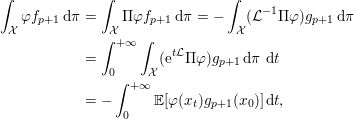


An alternative strategy consists in using a Metropolis–Hastings
algorithm with the numerical scheme as a proposal, in order to completely remove
the systematic error due to the time discretization. This is straightforward for
reversible dynamics such as overdamped Langevin dynamics. When an
Euler–Maruyama scheme is used, one obtains the so-called
Metropolis-adjusted Langevin algorithm (MALA) in the statistics literature, known
as smart MC in the chemistry literature (Rossky, Doll and Friedman Reference Rossky, Doll and Friedman1978, Roberts and Rosenthal Reference Roberts and Rosenthal1998). Another advantage of superimposing a
Metropolis–Hastings procedure upon a discretization of overdamped
Langevin dynamics is that it stabilizes the numerical scheme even for non-globally
Lipschitz forces  ${\rm\nabla}V$: an invariant probability measure exists by construction, which
ensures the recurrence of the Markov chain. In contrast, numerical discretizations
which are not stabilized by a Metropolis–Hastings procedure may be
transient, as discussed in Section 3.2.
For Langevin dynamics, some care has to be taken since the transition kernel associated with the Hamiltonian dynamics is irregular (because the noise acts only on momenta), which raises some difficulties in the definition of the Metropolis–Hastings ratio. It is nonetheless possible to use a Metropolis–Hastings procedure for schemes based on a splitting between the Ornstein–Uhlenbeck process on the momenta and a reversible discretization of the Hamiltonian part, upon reverting momenta when rejecting proposed moves; see Lelièvre et al. (Reference Lelièvre, Rousset and Stoltz2010, Section 2.2.3.2) for a precise discussion.
However, Metropolis corrections are usually not implemented in popular molecular dynamics packages such as NAMD since it is not always possible or desirable to use a Metropolis correction. First, the average acceptance probability in the Metropolis step for MALA or related algorithms in general decreases exponentially with the dimension of the system for a fixed time step. In fact, the time step should be reduced as some inverse power of the system size in order to maintain a constant acceptance rate (see Roberts, Gelman and Gilks Reference Roberts, Gelman and Gilks1997, Roberts and Rosenthal Reference Roberts and Rosenthal1998). There are two ways to limit the decrease of the acceptance probability.
(i) Change the dynamics or the measure used to compute the Metropolis ratio. For the Metropolization of the Hamiltonian dynamics, see the works by Izaguirre and Hampton (Reference Izaguirre and Hampton2004) and Akhmatskaya and Reich (Reference Akhmatskaya and Reich2005) where the Hamiltonian
$H$ in the canonical measure is changed to $H+{\rm\Delta}t^{2}\widetilde{H}$, with $\widetilde{H}$ the first-order correction arising from backward error
analysis. For the Metropolization of overdamped Langevin dynamics, see
Fathi and Stoltz (Reference Fathi and Stoltz2015).(ii) Evolve only subparts of the system (in the spirit of a Gibbs sampler), as advocated by Bou-Rabee and Vanden-Eijnden (Reference Bou-Rabee and Vanden-Eijnden2012).


However, the latter strategy may complicate the implementation of parallel
algorithms for the simulation of very large systems, especially if long-range
potentials are used (as acknowledged in Bou-Rabee and Vanden-Eijnden Reference Bou-Rabee and Vanden-Eijnden2012, Remark 2.5). Second, the
variance of the computed averages may increase since rejections occur, and the
samples along the numerical trajectory are therefore more correlated in general
than for rejection-free dynamics. Lastly, the Metropolis procedure requires that
the invariant measure  ${\it\pi}$ of the continuous dynamics is known. This is the case for
Langevin and overdamped Langevin dynamics with forces
 $-{\rm\nabla}V(q)$. However, for non-reversible systems subjected to external
forcings such as a temperature gradient or a non-gradient force (see
Section 5), the invariant
measure of the continuous dynamics is not known.
3.4 Variance reduction
As already mentioned in (3.14), the variance of trajectory averages computed with discretizations of SDEs are consistent with the variance of trajectory averages computed with the continuous dynamics they approximate. In this section we discuss standard ways to reduce this variance in order to decrease the statistical error in the estimated averages (3.10).
A first important distinction should be made between target-oriented variance
reduction, which corresponds to reducing the asymptotic variance  ${\it\varsigma}_{{\it\varphi}}^{2}$ defined in (3.5)
for a given observable
 ${\it\varphi}$; and a general-purpose reduction, for which the aim is to decrease
 $$\begin{eqnarray}\sup _{{\it\varphi}\in L^{2}({\it\pi})}\frac{{\it\varsigma}_{{\it\varphi}}^{2}}{\Vert {\it\varphi}\Vert _{L^{2}({\it\pi})^{2}}}=\sup _{\Vert {\it\varphi}\Vert _{L^{2}({\it\pi})}\leqslant 1}2\int _{{\mathcal{X}}}{\rm\Pi}{\it\varphi}(-{\mathcal{L}}^{-1}{\rm\Pi}{\it\varphi})\,\text{d}{\it\pi}.\end{eqnarray}$$
In (3.33), we
choose  ${\it\varphi}\in L^{2}({\it\pi})$ for simplicity, but the same question may be raised for specific
subsets of
 $L^{2}({\it\pi})$.
For Markov chains or Markov processes, the fact that the variance is large is due to the fact that the correlation time of the dynamics is large (see the discussion after (3.6)), which itself is due to the metastability of the process. The idea is therefore to modify the dynamics in order to remove, or at least reduce the metastability, while still being able to reconstruct canonical averages.
We present in this section standard variance reduction techniques for Markov processes. These techniques are extensions of methods used for i.i.d. sequences, for which a review is provided in Caflisch (Reference Caflisch1998). The most famous techniques are antithetic variables, stratification, control variate methods and importance sampling. We present flavours of the latter three approaches in this section.
3.4.1 Stratification
Stratification is a way of decomposing a difficult sampling problem into several easier ones. Ideally, the phase space should be decomposed into the collection of all metastable states, corresponding to local minima of the potential energy function, and these regions should be independently sampled. The local averages in each region should then be reweighted according to the canonical weight of the region itself. This method is therefore a general-purpose variance reduction technique.
There are two major ways to make this idea practical, depending on whether the considered regions overlap.
(i) When there is some overlap between the regions, bridge sampling methods such as MBAR (Shirts and Chodera Reference Shirts and Chodera2008) can be used. The method is based on several works in statistics (Geyer Reference Geyer1994, Meng and Wong Reference Meng and Wong1996, Kong et al. Reference Kong, McCullagh, Meng, Nicolae and Tan2003, Tan Reference Tan2004).
(ii) Non-overlapping regions can also be constructed as the level sets of some real-valued function of the configuration of the system. In this case, the sampling is performed by constraining the dynamics on the level set, and varying the constant defining the level set in order to sample the full phase space. This method is known as thermodynamic integration, with a reconstruction performed by computing the free energy: see Section 4.5.
3.4.2 Control variate
The control variate method is a classical technique for variance reduction,
although it is not so often used in molecular simulation. Consider the case when
thermodynamic averages such as (1.3) or (1.4) are
estimated by ergodic averages of a stochastic dynamics with generator  ${\mathcal{L}}$. Recall that we denote the invariant measure by
 ${\it\pi}$ and the configuration of the system by
 $x\in {\mathcal{X}}$, so that thermodynamic averages read
 $\mathbb{E}_{{\it\pi}}({\it\varphi})$.
Let us first explain the general principle of control variates applied to a simple
example. Consider a given observable  ${\it\varphi}$, and introduce an observable
 ${\it\phi}$ such that
 $\mathbb{E}_{{\it\pi}}({\it\phi})=0$. Then,
 $$\begin{eqnarray}\mathbb{E}_{{\it\pi}}({\it\varphi})=\mathbb{E}_{{\it\pi}}({\it\varphi}-{\it\phi}).\end{eqnarray}$$
The idea now is to choose  ${\it\phi}$ such that
 $\text{Var}_{{\it\pi}}({\it\varphi}-{\it\phi})$ is much smaller than
 $\text{Var}_{{\it\pi}}({\it\varphi})$. Of course, the optimal choice is
 ${\it\phi}={\it\varphi}-\mathbb{E}_{{\it\pi}}({\it\varphi})$, in which case
 $\text{Var}_{{\it\pi}}({\it\varphi}-{\it\phi})=0$. Note however that the optimal control variate depends on the
quantity of interest,
 $\mathbb{E}_{{\it\pi}}({\it\varphi})$, which is not available.
A systematic way of constructing admissible control variates (that is, functions
with average 0 with respect to  ${\it\pi}$) is to choose them in the image of the generator
 ${\mathcal{L}}$. Indeed, the invariance of the measure
 ${\it\pi}$, formulated as (1.17), leads to the following equality: for any
 $C^{\infty }$ and compactly supported test function
 ${\rm\Phi}$,
 $$\begin{eqnarray}\mathbb{E}_{{\it\pi}}({\it\varphi})=\mathbb{E}_{{\it\pi}}({\it\varphi}-{\mathcal{L}}{\rm\Phi})=\int _{{\mathcal{X}}}({\it\varphi}-{\mathcal{L}}{\rm\Phi})\,\text{d}{\it\pi}.\end{eqnarray}$$
The optimal choice corresponds to the solution of the Poisson equation
 $$\begin{eqnarray}{\mathcal{L}}{\rm\Phi}={\it\varphi}-\mathbb{E}_{{\it\pi}}({\it\varphi}).\end{eqnarray}$$
The solvability of this equation is ensured by
Corollaries 2.4, 2.16, 2.21 and 2.27, depending on the dynamics at hand and/or the integrability
properties of the observable  ${\it\varphi}$ under consideration. By construction, the estimator based on
(3.34)–(3.35), namely
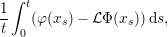 $$\begin{eqnarray}\frac{1}{t}\int _{0}^{t}({\it\varphi}(x_{s})-{\mathcal{L}}{\rm\Phi}(x_{s}))\,\text{d}s,\end{eqnarray}$$
has a variance equal to 0 since  ${\it\varphi}(x)-{\mathcal{L}}{\rm\Phi}(x)=\mathbb{E}_{{\it\pi}}({\it\varphi})$ for any value of
 $x\in {\mathcal{X}}$. Such approaches were first suggested for Markov chains in the
computational statistics literature (Andradóttir, Heyman and Ott Reference Andradóttir, Heyman and Ott1993, Henderson Reference Henderson1997) but have also been proposed in the statistical physics
literature (Assaraf and Caffarel Reference Assaraf and Caffarel1999),
where they are known as the ‘zero-variance principle’.
In practice, it is generally impossible to solve the Poisson equation (3.35) exactly. However, it is
possible to approximate the ideal function  ${\rm\Phi}$ in (3.35) on a
basis of
 $K$ trial functions
 ${\rm\Phi}_{1},\ldots ,{\rm\Phi}_{K}$. This amounts to optimizing the coefficients
 $a=(a_{1},\ldots ,a_{K})\in \mathbb{R}^{K}$ such that the variance of the estimator
 $$\begin{eqnarray}\widehat{{\it\varphi}}_{t}(a_{1},\ldots ,a_{K})=\frac{1}{t}\int _{0}^{t}{\it\phi}_{a_{1},\ldots ,a_{K}}(x_{s})\,\text{d}s,\quad {\it\phi}_{a_{1},\ldots ,a_{K}}={\it\varphi}-\mathop{\sum }_{k=1}^{K}a_{k}{\mathcal{L}}{\rm\Phi}_{k}\end{eqnarray}$$
is minimal.
3.4.3 Importance sampling
The basic idea of importance sampling is to change the measure which is sampled
into a measure which is easier to sample. In the context of molecular simulation,
this is most commonly done by changing the potential energy function  $V$ in the dynamics to a modified potential
 $V+\widetilde{V}$. However, there are alternative strategies: see for instance
Redon et al. (Reference Redon, Stoltz and Trstanova2016), where the kinetic energy function is modified for Langevin
dynamics. The modified overdamped Langevin dynamics associated with the potential
 $V+\widetilde{V}$, namely
 $$\begin{eqnarray}\text{d}q_{t}=-{\rm\nabla}(V+\widetilde{V})(q_{t})\,\text{d}t+\sqrt{\frac{2}{{\it\beta}}}\,\text{d}W_{t},\end{eqnarray}$$
is then ergodic for the modified probability measure 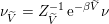 ${\it\nu}_{\widetilde{V}}=Z_{\widetilde{V}}^{-1}\,\text{e}^{-{\it\beta}\widetilde{V}}{\it\nu}$. Likewise, the modified Langevin dynamics
 $$\begin{eqnarray}\displaystyle \text{d}\widetilde{q}_{t} & = & \displaystyle M^{-1}\widetilde{p}_{t}\,\text{d}t,\nonumber\\ \displaystyle \text{d}\widetilde{p}_{t} & = & \displaystyle -{\rm\nabla}(V+\widetilde{V})(\widetilde{q}_{t})\,\text{d}t-{\it\gamma}\,M^{-1}\widetilde{p}_{t}\,\text{d}t+\sqrt{\frac{2{\it\gamma}}{{\it\beta}}}\,\text{d}W_{t}\nonumber\end{eqnarray}$$
is ergodic for the modified canonical probability measure 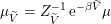 ${\it\mu}_{\widetilde{V}}=Z_{\widetilde{V}}^{-1}\,\text{e}^{-{\it\beta}\widetilde{V}}{\it\mu}$. The fundamental observation to retrieve averages with respect to
 ${\it\nu}$ or
 ${\it\mu}$ with realizations of the modified dynamics is that
 $$\begin{eqnarray}\int _{{\mathcal{D}}}{\it\varphi}(q)\,{\it\nu}(\text{d}q)=\int _{{\mathcal{E}}}{\it\varphi}(q)\,{\it\mu}(\text{d}q\,\text{d}p)=\frac{\int _{{\mathcal{D}}}{\it\varphi}\,\text{e}^{{\it\beta}\widetilde{V}}\,\text{d}{\it\nu}_{\widetilde{V}}}{\int _{{\mathcal{D}}}\,\text{e}^{{\it\beta}\widetilde{V}}\,\text{d}{\it\nu}_{\widetilde{V}}}=\frac{\int _{{\mathcal{E}}}{\it\varphi}\,\text{e}^{{\it\beta}\widetilde{V}}\,\text{d}{\it\mu}_{\widetilde{V}}}{\int _{{\mathcal{E}}}\,\text{e}^{{\it\beta}\widetilde{V}}\,\text{d}{\it\mu}_{\widetilde{V}}}.\end{eqnarray}$$
Therefore, the following estimator is considered:
 $$\begin{eqnarray}\widehat{{\it\varphi}}_{t}^{\widetilde{V}}=\frac{\int _{0}^{t}{\it\varphi}(\widetilde{q}_{s})\,\text{e}^{{\it\beta}\widetilde{V}(\widetilde{q}_{s})}\,\text{d}s}{\int _{0}^{t}\,\text{e}^{{\it\beta}\widetilde{V}(\widetilde{q}_{s})}\,\text{d}s}.\end{eqnarray}$$
After discretization in time, the estimator  $\widehat{{\it\varphi}}_{t}^{\widetilde{V}}$ is approximated by
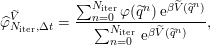 $$\begin{eqnarray}\widehat{{\it\varphi}}_{N_{\text{iter}},{\rm\Delta}t}^{\widetilde{V}}=\frac{\mathop{\sum }_{n=0}^{N_{\text{iter}}}{\it\varphi}(\widetilde{q}^{n})\,\text{e}^{{\it\beta}\widetilde{V}(\widetilde{q}^{n})}}{\mathop{\sum }_{n=0}^{N_{\text{iter}}}\,\text{e}^{{\it\beta}\widetilde{V}(\widetilde{q}^{n})}},\end{eqnarray}$$
where  $\widetilde{q}^{n}$ is an approximation of
 $\widetilde{q}_{n{\rm\Delta}t}$.
In order for importance sampling to be efficient, the weights  $\text{e}^{{\it\beta}\widetilde{V}(q^{n})}$ should not be too degenerate. This can be quantified in various
ways, for instance through the so-called efficiency factor
 $$\begin{eqnarray}\frac{(\mathop{\sum }_{n=0}^{N_{\text{iter}}}\,\text{e}^{{\it\beta}\widetilde{V}(q^{n})})^{2}}{N_{\text{iter}}\mathop{\sum }_{n=0}^{N_{\text{i ter }}}\,\text{e}^{2{\it\beta}\widetilde{V}(q^{n})}}\in [0,1].\end{eqnarray}$$
The fact that this number is indeed between 0 and 1 can be seen via the Cauchy–Schwarz inequality. The efficiency factor counts the fraction of significant values on average. It should be as close as possible to 1, which is indeed the case if the weights are of similar magnitudes. In the statistics literature, the efficiency factor corresponds to the effective sample size of Kong, Liu and Wong (Reference Kong, Liu and Wong1994) divided by the number of sampled values.
When the observable  ${\it\varphi}$ under consideration is fixed (target-oriented variance
reduction), it is possible to optimize the importance sampling procedure in order
to minimize the variance of the estimator. We illustrate this fact for samples
 $\widetilde{q}^{n}$ independently and identically distributed from a measure with
density
 $\text{e}^{-{\it\beta}(V(q)+\widetilde{V}(q))}$, whose normalization constant fortunately does not need to be
known. Consider the estimator
 $$\begin{eqnarray}\widehat{{\it\varphi}}_{N_{\text{iter}}}^{\text{iid},\widetilde{V}}=\frac{\mathop{\sum }_{n=0}^{N_{\text{iter}}}{\it\varphi}(\widetilde{q}^{n})\,\text{e}^{{\it\beta}\widetilde{V}(\widetilde{q}^{n})}}{\mathop{\sum }_{n=0}^{N_{\text{i ter }}}\,\text{e}^{{\it\beta}\widetilde{V}(\widetilde{q}^{n})}},\quad \widetilde{q}^{n}\sim {\it\nu}_{\widetilde{V}}~~\text{i.i.d.}\end{eqnarray}$$
A simple computation based on the equalityFootnote 9  ${\it\nu}_{\widetilde{V}}/{\it\nu}=\text{e}^{-{\it\beta}\widetilde{V}}\,Z_{0}/Z_{\widetilde{V}}$ shows that
 $$\begin{eqnarray}\sqrt{N_{\text{iter}}}(\widehat{{\it\varphi}}_{N_{\text{iter}}}^{\text{iid},\widetilde{V}}-\mathbb{E}_{{\it\nu}}({\it\varphi}))=\frac{\sqrt{N_{\text{iter}}}[\frac{1}{N_{\text{i ter }}}\mathop{\sum }_{n=0}^{N_{\text{iter}}}[{\it\varphi}(\widetilde{q}^{n})-\mathbb{E}_{{\it\nu}}({\it\varphi})]\frac{{\it\nu}}{{\it\nu}_{\widetilde{V}}}(\widetilde{q}^{n})]}{\frac{1}{N_{\text{iter}}}\mathop{\sum }_{n=0}^{N_{\text{iter}}}\frac{{\it\nu}}{{\it\nu}_{\widetilde{V}}}(\widetilde{q}^{n})}.\end{eqnarray}$$
By the law of large numbers, the denominator almost surely
converges to 1 as  $N_{\text{iter}}\rightarrow +\infty$, while, by the central limit theorem, the numerator converges in
law to a Gaussian distribution with variance
 $$\begin{eqnarray}{\it\varsigma}_{\widetilde{V}}^{2}({\it\varphi})=\int _{{\mathcal{D}}}\frac{({\rm\Pi}{\it\varphi})^{2}{\it\nu}^{2}}{{\it\nu}_{\widetilde{V}}},\end{eqnarray}$$
where we introduced  ${\rm\Pi}{\it\varphi}={\it\varphi}-\mathbb{E}_{{\it\nu}}({\it\varphi})$. By Slutsky’s theorem, the random variable
 $$\begin{eqnarray}\sqrt{N_{\text{iter}}}(\widehat{{\it\varphi}}_{N_{\text{iter}}}^{\text{iid},\widetilde{V}}-\mathbb{E}_{{\it\nu}}({\it\varphi}))\end{eqnarray}$$
therefore converges in law to a Gaussian distribution with
variance  ${\it\varsigma}_{\widetilde{V}}^{2}({\it\varphi})$. The Cauchy–Schwarz inequality on
 $L^{2}({\it\nu}_{\widetilde{V}})$ now shows that
 $$\begin{eqnarray}{\it\varsigma}_{\widetilde{V}}^{2}({\it\varphi})\geqslant \biggl(\int _{{\mathcal{D}}}\frac{|{\rm\Pi}{\it\varphi}|{\it\nu}}{{\it\nu}_{\widetilde{V}}}\,{\it\nu}_{\widetilde{V}}\biggr)^{2}=\biggl(\int _{{\mathcal{D}}}|{\rm\Pi}{\it\varphi}|\,\text{d}{\it\nu}\biggr)^{2},\end{eqnarray}$$
with equality if and only if  $|{\rm\Pi}{\it\varphi}|{\it\nu}/{\it\nu}_{\widetilde{V}}\propto 1$. The optimal biased measure for i.i.d. sampling is
thus
 $$\begin{eqnarray}{\it\nu}_{\widetilde{V}}(\text{d}q)=\frac{|{\rm\Pi}{\it\varphi}(q)|\,{\it\nu}(\text{d}q)}{\int _{{\mathcal{D}}}|{\rm\Pi}{\it\varphi}|\,\text{d}{\it\nu}}\end{eqnarray}$$
which formally corresponds to the potential
 $$\begin{eqnarray}\widetilde{V}(q)=-\frac{1}{{\it\beta}}\log |{\rm\Pi}{\it\varphi}(q)|.\end{eqnarray}$$
The latter expression is singular at configurations  $q$ such that
 ${\rm\Pi}{\it\varphi}(q)=0$. More importantly, the expression of
 $\widetilde{V}$ depends on
 $\mathbb{E}_{{\it\nu}}({\it\varphi})$, and is therefore not available as such. We will extend such
importance sampling approaches to averages over the path space in
Section 6.2, and will also
show how to approximate the optimal bias in this context.
Let us finally discuss general-purpose variance reduction in the context of
importance sampling. In view of the definition (3.33), a reduction in the variance
for any observable  ${\it\varphi}$ amounts to a decrease in the operator norm of the
symmetric part of
 ${\mathcal{L}}^{-1}$. Note indeed that only the symmetric part of of
 ${\mathcal{L}}^{-1}$ matters in the right-hand side of (3.33). For overdamped Langevin
dynamics, the generator is self-adjoint:
 ${\mathcal{L}}={\mathcal{L}}^{\ast }$ when these operators are considered on
 $L^{2}({\it\nu})$. General variance reduction therefore amounts to increasing the
spectral gap of the operator (see (2.82)). This can be done by choosing
 $\widetilde{V}$ to erase local minima in
 $V$ which degrade the Poincaré/LSI constants (see
Section 2.2). In
Section 4 we discuss good
choices of
 $\widetilde{V}$ to overcome such metastability issues. When the generator
 ${\mathcal{L}}$ is not self-adjoint, there are a priori no
simple relationships between the symmetric and antisymmetric parts of
 ${\mathcal{L}}$ and its inverse. However, some results can be obtained for
specific dynamics, such as overdamped Langevin dynamics perturbed by a
divergence-free non-reversible drift: see Duncan, Lelièvre
and Pavliotis (Reference Duncan, Lelièvre and Pavliotis2016) and Rey-Bellet and
Spiliopoulos (Reference Rey-Bellet and Spiliopoulos2016).
4 Free energy computations and adaptive importance sampling methods
This section is devoted to presentation of a sampling method of the canonical measure, which was developed in the field of molecular dynamics but could also be used in many other contexts. As explained in Section 1.2, sampling the canonical measure is difficult because the dimension is large, and the measure is multimodal. The high-dimensionality of the problem entails the use of stochastic dynamics to sample the target measure, and the multimodality of the target implies the metastability of the process (and thus the slow convergence of time averages). In this section we present techniques which circumvent the difficulties raised by the metastability of the sampling dynamics, by using two ideas.
∙ Use an importance sampling method (see Section 3.4.3) by changing the original potential
$V$ toFootnote 10 $V-F\circ {\it\xi}$, where $F$ is the so-called free energy associated with the reaction
coordinate ${\it\xi}$ (see Section 4.1 for precise definitions).∙ Since the free energy is not available in practice, instead of the biasing potential
$F\circ {\it\xi}$, an approximation $F_{t}\circ {\it\xi}$ is used, where $F_{t}$ is an estimate of the free energy at time $t$, given all the configurations visited so far: $F_{t}$ is updated on-the-fly in order to better approximate the free
energy $F$ as time goes on (this is the adaptive feature of the
approach).


Methods of this type are thus called free energy adaptive biasing techniques, and encompass many algorithms (Lelièvre, Rousset and Stoltz Reference Lelièvre, Rousset and Stoltz2007): the adaptive biasing force (Darve and Porohille Reference Darve and Porohille2001, Hénin and Chipot Reference Hénin and Chipot2004), the Wang–Landau algorithm (Wang and Landau Reference Wang and Landau2001a, Wang and Landau Reference Wang and Landau2001b), metadynamics (Laio and Parrinello Reference Laio and Parrinello2002, Bussi, Laio and Parrinello Reference Bussi, Laio and Parrinello2006), and the self-healing umbrella sampling method (Marsili et al. Reference Marsili, Barducci, Chelli, Procacci and Schettino2006, Dickson et al. Reference Dickson, Legoll, Lelièvre, Stoltz and Fleurat-Lessard2010).
This section is organized as follows. In Section 4.1 we introduce the notion of free energy. In Section 4.2 we present in detail the two families of adaptive techniques: adaptive biasing potential (ABP) and adaptive biasing force (ABF) methods, in a rather general setting. Section 4.3 is devoted to the mathematical analysis of an ABF approach based on entropy techniques and logarithmic Sobolev inequalities (in the spirit of the techniques introduced in Section 2.2). For pedagogical purposes, this mathematical analysis is presented in a simple setting. Extensions and related works are mentioned in Section 4.4. The focus of this section is thus on adaptive techniques. We will show in particular how an analysis based on partial differential equations is very useful for understanding the efficiency of the methods. However, we will also give a quick overview of other free energy calculation techniques in Section 4.5.
4.1 Free energy
4.1.1 Reaction coordinate
In order to introduce the notions of free energy and reaction coordinate, let us
go back to the simple two-dimensional experiments of Section 1.2 reported in Figure 1.1. On the time evolution of the  $x$-coordinate of the stochastic process, one observes metastable
features: the process remains trapped for a very long time in some interval around
 $-1$ before hopping to another metastable region, around
 $1$. The transition between the two metastable states can be
inferred from the time evolution of the
 $x$-coordinate. The
 $x$-coordinate is thus a slow variable of the system, in the sense
that the typical time scale on which hopping events occur is much larger than the
typical time scale of vibrations within metastable regions. In this simple
two-dimensional example, a reaction coordinate is thus the function
 ${\it\xi}(x,y)=x$ (where we let
 $(x,y)$ denote the two components of the position
 $q$). Generally speaking, a reaction coordinate is a function
 $$\begin{eqnarray}{\it\xi}:\mathbb{R}^{d}\rightarrow \mathbb{R}^{m}\end{eqnarray}$$
with  $m\leqslant d$, such that
 $({\it\xi}(q_{t}))_{t\geqslant 0}$ is a metastable process. Here and in the following, we assume
for simplicity that the position space
 ${\mathcal{D}}$ is
 $\mathbb{R}^{d}$, but the generalization to a general space
 ${\mathcal{D}}$ is straightforward. The function
 ${\it\xi}$ thus indexes the transitions between some metastable states. In
addition we require the dimension
 $m$ of the reaction coordinate to be as small as possible, in order
to have a low-dimensional representation of the original high-dimensional system
via
 $({\it\xi}(q_{t}))_{t\geqslant 0}$ (for the numerical methods presented in this section,
 $m$ is typically required to be less than
 $4$, even though some methods have been proposed to deal with
higher-dimensional reaction coordinates; see for example Piana and Laio Reference Piana and Laio2007). In practice, it could be an angle in a
protein, for instance, which characterizes the conformation of the molecule, or
the position of a defect in a material. For choosing a reaction coordinate
 ${\it\xi}$, the practitioner needs some a priori knowledge of
the system, since the reaction coordinate should characterize the conformations of
the system which correspond to some metastable states of the dynamics.
4.1.2 Free energy
Once a reaction coordinate  ${\it\xi}$ has been chosen, one can introduce the free energy associated
with
 ${\it\xi}$. Let us again go back to the simple two-dimensional example of
Figure 1.1, and to the specific
choice
 ${\it\xi}(x,y)=x$. One can define the marginal distribution of
 $$\begin{eqnarray}{\it\nu}(\text{d}x\text{d}y)=Z_{{\it\nu}}^{-1}\exp (-{\it\beta}V(x,y))\,\text{d}x\,\text{d}y,\end{eqnarray}$$
in  $x$, namely the probability measure on
 $\mathbb{R}$:
 $$\begin{eqnarray}\biggl(Z_{{\it\nu}}^{-1}\int _{\mathbb{R}}\exp (-{\it\beta}V(x,y))\,\text{d}y\biggr)\,\text{d}x.\end{eqnarray}$$
Notice that the integration is performed only over  $y$ in the previous definition. Then, the free energy
 $F(x)$ is defined so that
 $\exp (-{\it\beta}F(x))$ is the density of this marginal law:
 $$\begin{eqnarray}F(x)=-{\it\beta}^{-1}\ln \biggl(Z_{{\it\nu}}^{-1}\int _{\mathbb{R}}\exp (-{\it\beta}V(x,y))\,\text{d}y\biggr).\end{eqnarray}$$
In a more general setting, a similar definition holds.
Definition 4.1 (free energy).
The free energy  $F:\mathbb{R}^{m}\rightarrow \mathbb{R}$ associated with the canonical measure
 ${\it\nu}(\text{d}q)=Z_{{\it\nu}}^{-1}\exp (-{\it\beta}V(q))\,\text{d}q$ and the reaction coordinate
 ${\it\xi}:\mathbb{R}^{d}\rightarrow \mathbb{R}^{m}$ is defined by
 $$\begin{eqnarray}F(z)=-{\it\beta}^{-1}\ln \biggl(\int _{{\rm\Sigma}(z)}\exp (-{\it\beta}V(q)){\it\delta}_{{\it\xi}(q)-z}(\text{d}q)\biggr),\quad \text{for all }z\in \mathbb{R}^{m},\end{eqnarray}$$
where  ${\rm\Sigma}(z)=\{q\in \mathbb{R}^{d},\,{\it\xi}(q)=z\}$.
The free energy  $F$ (as the potential
 $V$) is actually defined up to an additive constant, and is such
that
 $Z_{F}^{-1}\exp (-{\it\beta}F(z))\,\text{d}z$, where
 $$\begin{eqnarray}Z_{F}=\int _{\mathbb{R}^{m}}\exp (-{\it\beta}F(z))\,\text{d}z=Z_{{\it\nu}},\end{eqnarray}$$
by definition (4.1), is the image of the measure  ${\it\nu}$ by
 ${\it\xi}$ (or equivalently the marginal distribution of
 ${\it\nu}$ along
 ${\it\xi}$). Since the free energy
 $F$ is defined up to an additive constant, quantities of interest
are actually free energy differences between two states indexed by
 ${\it\xi}$.
In Definition 4.1, we
used the delta measure  ${\it\delta}_{{\it\xi}(q)-z}(\text{d}q)$, which is a measure supported by the submanifold
 ${\rm\Sigma}(z)$. One way to define this measure is the following: the delta
measure
 ${\it\delta}_{{\it\xi}(q)-z}(\text{d}q)$ is such that ‘
 ${\it\delta}_{{\it\xi}(q)-z}(\text{d}q)\,\text{d}z=\text{d}q$’. More precisely, for all
 $C^{\infty }$ and compactly supported test functions
 $A:\mathbb{R}^{m}\rightarrow \mathbb{R}$ and
 $B:\mathbb{R}^{d}\rightarrow \mathbb{R}$,
 $$\begin{eqnarray}\int _{\mathbb{R}^{d}}A\circ {\it\xi}(q)B(q)\,\text{d}q=\int _{\mathbb{R}^{m}}A(z)\biggl(\int _{{\rm\Sigma}(z)}B(q){\it\delta}_{{\it\xi}(q)-z}(\text{d}q)\biggr)\,\text{d}z.\end{eqnarray}$$
The delta measure can be understood using a regularization
procedure: for any  $C^{\infty }$ and compactly supported test function
 $A:\mathbb{R}^{d}\rightarrow \mathbb{R}$,
 $$\begin{eqnarray}\int _{{\rm\Sigma}(z)}A(q){\it\delta}_{{\it\xi}(q)-z}(\text{d}q)=\lim _{{\it\varepsilon}\rightarrow 0}\int _{\mathbb{R}^{d}}A(q){\it\delta}^{{\it\varepsilon}}({\it\xi}(q)-z)\,\text{d}q,\end{eqnarray}$$
where  ${\it\delta}^{{\it\varepsilon}}$ is a
 $C^{\infty }$ approximation of the identity (when
 ${\it\varepsilon}\rightarrow 0$,
 ${\it\delta}^{{\it\varepsilon}}$ converges to the Dirac in the sense of distributions).
Remark 4.2 (co-area formula).
The delta measure can also be defined in terms of the surface measure  ${\it\sigma}_{{\rm\Sigma}(z)}$ over the submanifold
 ${\rm\Sigma}(z)\subset \mathbb{R}^{d}$, equipped with the Riemannian structure from
 $\mathbb{R}^{d}$:
 $$\begin{eqnarray}{\it\delta}_{{\it\xi}(q)-z}(\text{d}q)=(\det G)^{-1/2}\,\text{d}{\it\sigma}_{{\rm\Sigma}(z)},\end{eqnarray}$$
where
 $$\begin{eqnarray}G=({\rm\nabla}{\it\xi})^{T}{\rm\nabla}{\it\xi},\end{eqnarray}$$
which has components
 $$\begin{eqnarray}G_{{\it\alpha},{\it\beta}}={\rm\nabla}{\it\xi}_{{\it\alpha}}\cdot {\rm\nabla}{\it\xi}_{{\it\beta}},\quad \text{for all }({\it\alpha},{\it\beta})\in \{1,\ldots ,m\}^{2}.\end{eqnarray}$$
The equivalence between this definition and the previous one
is a consequence of the co-area formula (Ambrosio, Fusco and Pallara Reference Ambrosio, Fusco and Pallara2000, Evans and Gariepy Reference Evans and Gariepy1992, Lelièvre
et al. Reference Lelièvre, Rousset and Stoltz2010). Note that it is implicitly
assumed here and in the following that  $\det G\neq 0$ (where
 $G$ is defined by (4.3)). Contrary to the surface measure
 ${\it\sigma}_{{\rm\Sigma}(z)}$, the measure
 ${\it\delta}_{{\it\xi}(q)-z}(\text{d}z)$ does not only depend on
 ${\it\xi}$ via its level set
 ${\rm\Sigma}(z)$, but also depends on the value of
 ${\rm\nabla}{\it\xi}$ over
 ${\rm\Sigma}(z)$. Note that in the simple case where
 $m=1$ (one-dimensional reaction coordinate),
 $\det G=|{\rm\nabla}{\it\xi}|^{2}$. Further, when
 ${\it\xi}(q_{1},\ldots ,q_{d})=(q_{1},\ldots ,q_{m})$, then
 $\det G=1$ and
 ${\it\delta}_{{\it\xi}(q)-z}(\text{d}q)=\text{d}q_{m+1}\cdots \text{d}q_{n}$ is simply the surface measure on the hyperplane
 $$\begin{eqnarray}{\rm\Sigma}(z)=\{q\in \mathbb{R}^{d},\,(q_{1},\ldots ,q_{m})=(z_{1},\ldots ,z_{m})\}.\end{eqnarray}$$
Once  $F$ has been defined by (4.1), the fact that
 $Z_{F}^{-1}\exp (-{\it\beta}F(z))\,\text{d}z$ is the image of the measure
 ${\it\nu}$ by
 ${\it\xi}$ is actually a direct consequence of (4.2). Indeed, for any
 $C^{\infty }$ and compactly supported test functions
 $A:\mathbb{R}^{m}\rightarrow \mathbb{R}$ and
 $B:\mathbb{R}^{d}\rightarrow \mathbb{R}$,
 $$\begin{eqnarray}\displaystyle & & \displaystyle \mathbb{E}_{{\it\nu}}(A({\it\xi}(q))B(q))=\int _{\mathbb{R}^{d}}A\circ {\it\xi}(q)B(q)Z_{{\it\nu}}^{-1}\exp (-{\it\beta}V(q))\,\text{d}q\nonumber\\ \displaystyle & & \displaystyle \quad =\int _{\mathbb{R}^{m}}A(z)\biggl(\int _{{\rm\Sigma}(z)}B(q)Z_{{\it\nu}}^{-1}\exp (-{\it\beta}V(q)){\it\delta}_{{\it\xi}(q)-z}(\text{d}q)\biggr)\,\text{d}z\nonumber\\ \displaystyle & & \displaystyle \quad =\int _{\mathbb{R}^{m}}A(z)\frac{\int _{{\rm\Sigma}(z)}B(q)Z_{{\it\nu}}^{-1}\exp (-{\it\beta}V(q)){\it\delta}_{{\it\xi}(q)-z}(\text{d}q)}{Z_{F}^{-1}\exp (-{\it\beta}F(z))}Z_{F}^{-1}\exp (-{\it\beta}F(z))\,\text{d}z.\nonumber\end{eqnarray}$$
Note that
 $$\begin{eqnarray}Z_{F}^{-1}\exp (-{\it\beta}F(z))=\int _{{\rm\Sigma}(z)}Z_{{\it\nu}}^{-1}\exp (-{\it\beta}V(q)){\it\delta}_{{\it\xi}(q)-z}(\text{d}q),\end{eqnarray}$$
so the fraction in the above integral defines the average of  $B$ with respect to a probability measure supported by
 ${\rm\Sigma}(z)$. More precisely, from this formula, one immediately gets that
the marginal law of
 ${\it\nu}$ along
 ${\it\xi}$ is
 $Z_{F}^{-1}\exp (-{\it\beta}F(z))$, and that the conditional probability of
 ${\it\nu}$, given that
 ${\it\xi}(x)=z$, is given by
 $$\begin{eqnarray}{\it\nu}(\text{d}q|{\it\xi}(q)=z)=\frac{Z_{{\it\nu}}^{-1}\exp (-{\it\beta}V(q)){\it\delta}_{{\it\xi}(q)-z}(\text{d}q)}{Z_{F}^{-1}\exp (-{\it\beta}F(z))}.\end{eqnarray}$$
Observe that, up to an additive constant,
 $$\begin{eqnarray}F(z)=-{\it\beta}^{-1}\ln Z_{z},\end{eqnarray}$$
where
 $$\begin{eqnarray}Z_{z}=\int _{{\rm\Sigma}(z)}Z_{{\it\nu}}^{-1}\exp (-{\it\beta}V(q)){\it\delta}_{{\it\xi}(q)-z}(\text{d}q)\end{eqnarray}$$
is the partition function of the probability measure  ${\it\nu}(\text{d}q|{\it\xi}(q)=z)$. This justifies the name ‘free energy’
(see Lelièvre et al. Reference Lelièvre, Rousset and Stoltz2010, Section 1.3.1.2).
As a consequence, the free energy  $F$ can be seen as a ‘coarse-grained’
potential function (for the degrees of freedom
 ${\it\xi}(q)$), which is thermodynamically consistent with the original
Boltzmann–Gibbs measure
 ${\it\nu}$, since the Boltzmann–Gibbs measure associated with
 $F$ (i.e.
 $Z_{F}^{-1}\exp (-{\it\beta}F(z))\,\text{d}z$) is exactly the marginal law of
 ${\it\nu}$ along
 ${\it\xi}$. In fact, computing the free energy is now the aim of many
molecular dynamics simulations (see Chipot and Pohorille Reference Chipot and Pohorille2007), since it gives a reduced description of the system
along specific degrees of freedom (the reaction coordinate).
4.2 Free energy adaptive biasing techniques
Let us now discuss why the free energy is useful for sampling purposes.
4.2.1 Free energy biased dynamics
As explained above, the main idea of free energy biasing techniques is to use an
importance sampling approach by replacing the original potential  $V$ by the biased potential
 $V-F\circ {\it\xi}$, where
 $F$ is the free energy associated with the reaction coordinate
 ${\it\xi}$. The intuition behind this idea is that by doing so, the
metastable features of the original potential along
 ${\it\xi}$ will be removed. Indeed, by the very definition of
 $F$, the marginal of the Boltzmann–Gibbs distribution
 $Z^{-1}\exp (-{\it\beta}(V-F\circ {\it\xi})(q))\,\text{d}q$ in
 ${\it\xi}$ has density
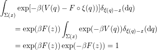 $$\begin{eqnarray}\displaystyle & & \displaystyle \int _{{\rm\Sigma}(z)}\exp [-{\it\beta}(V(q)-F\circ {\it\xi}(q))]{\it\delta}_{{\it\xi}(q)-z}(\text{d}q)\nonumber\\ \displaystyle & & \displaystyle \qquad =\exp ({\it\beta}F(z))\int _{{\rm\Sigma}(z)}\exp (-{\it\beta}V(q)){\it\delta}_{{\it\xi}(q)-z}(\text{d}q)\nonumber\\ \displaystyle & & \displaystyle \qquad =\exp ({\it\beta}F(z))\exp (-{\it\beta}F(z))=1\end{eqnarray}$$
(up to a normalizing constant). This means that along  ${\it\xi}$ the biased measure
 $Z^{-1}\exp (-{\it\beta}(V-F\circ {\it\xi})(q))\,\text{d}q$ is uniform. For the normalizing constant
 $Z=\int _{\mathbb{R}^{d}}\exp (-{\it\beta}(V-F\circ {\it\xi})(q))\,\text{d}q$ to be finite, one needs to consider a situation where
 ${\it\xi}$ lives in a compact space (for example the torus if one thinks of
an angle as a reaction coordinate) or to restrict the bias to a compact domain of
 $\mathbb{R}^{m}$. The idea is thus as follows. If the free energy
 $F$ were known, it would be a good biasing potential since the
biased Boltzmann–Gibbs measure
 $Z^{-1}\exp (-{\it\beta}(V-F\circ {\it\xi})(q))\,\text{d}q$ has a marginal law in
 ${\it\xi}$ which is the uniform law. It is thus expected that the
associated sampling dynamics (say Langevin or overdamped Langevin with
 $V-F\circ {\it\xi}$ as a potential) will no longer be metastable along the reaction
coordinate
 ${\it\xi}$.
To be compared with Figure 1.1. (a, b) Energetic barrier case,
(c, d) entropic barrier case. (a) Level
sets of the free energy biased potential. (b) Time evolution
of the  $x$-coordinate on the biased potential (
 ${\it\beta}=4$). (c) Free energy. (d) Time
evolution of the
 $x$-coordinate on the biased potential (
 ${\it\beta}=10$).
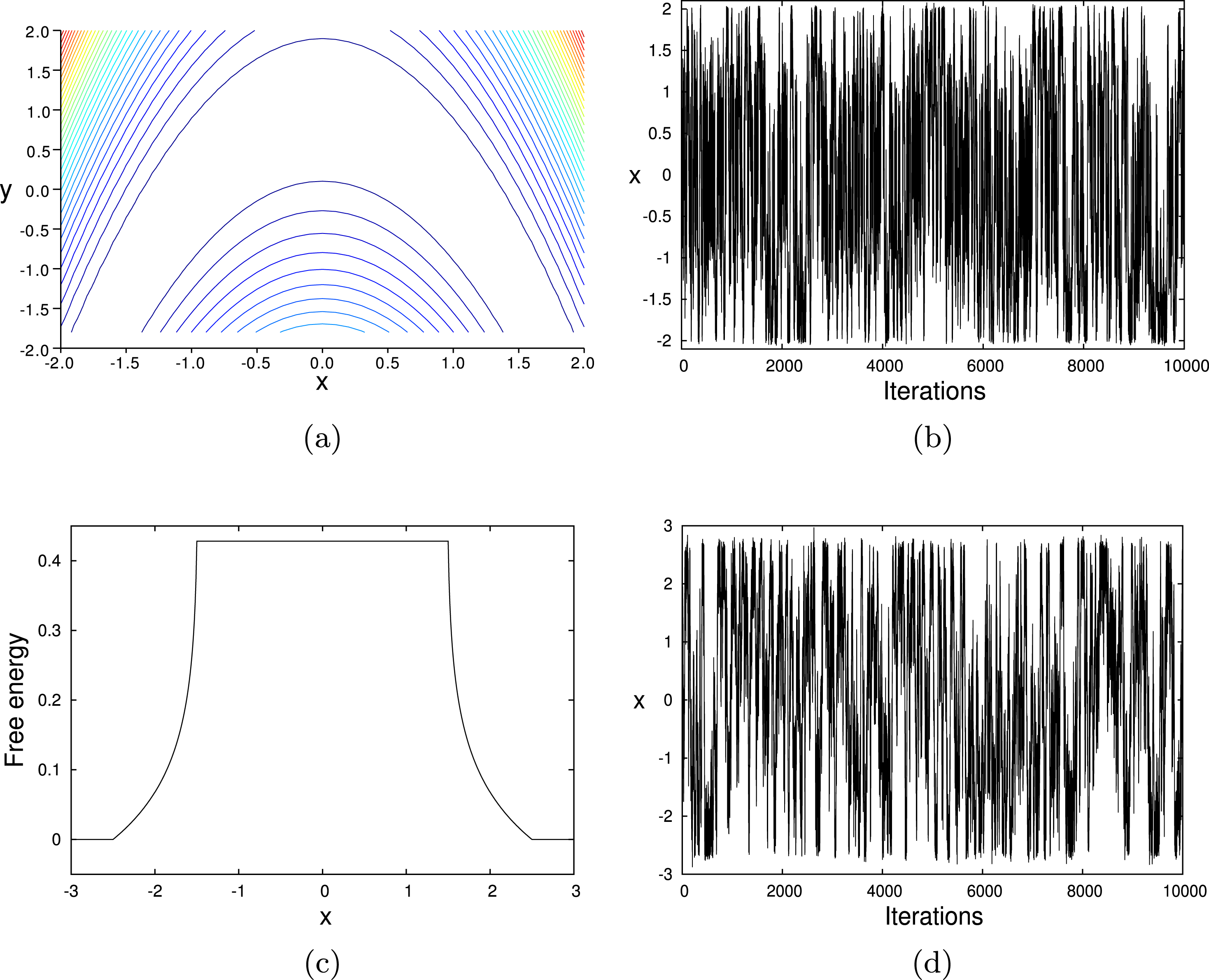
Before explaining how to make this idea practical by changing  $F$ to an approximation of
 $F$ in the previous reasoning, let us check that
 $F$ is indeed a good biasing potential on the simple two-dimensional
examples we considered in Section 1.2. In Figure 4.1 we
again plot the
 $x$-coordinate for overdamped Langevin dynamics as a function of
time, but using the biased potential
 $V-F\circ {\it\xi}$ instead of the original potential
 $V$, with
 ${\it\xi}(x,y)=x$ as a reaction coordinate. In these simple two-dimensional
examples, the free energy can be very easily computed by a simple integration in
 $y$, for a fixed value of
 $x$. By comparing the results with those of Figure 1.1, it is obvious that the biased dynamics
yields a much better coverage of the configuration space: the system now freely
moves from
 $x=-1$ to
 $x=1$, both in the energetic and the entropic barrier cases.
4.2.2 Updating formulae
Let us now explain the second key idea of free energy adaptive biasing techniques,
namely the adaptive feature of these numerical methods. As explained above, we
would like to use  $V-F\circ {\it\xi}$ as a potential instead of
 $V$. The problem is that
 $F$ is unknown (it is actually the aim of many molecular dynamics
computations to compute
 $F$). The idea is then to use
 $V-F_{t}\circ {\it\xi}$ as a potential, and to update
 $F_{t}$ in such a way that
 $F_{t}$ better approximates
 $F$ as time goes on.
There are two different strategies. Adaptive biasing potential (ABP) techniques
rely on the following formula for  $F$:
 $$\begin{eqnarray}\exp (-{\it\beta}F(z))=\int _{{\rm\Sigma}(z)}\exp (-{\it\beta}V(q)){\it\delta}_{{\it\xi}(q)-z}(\text{d}q),\quad \text{for all }z\in \mathbb{R}^{m}.\end{eqnarray}$$
Thus an approximation of  $F$ at time
 $t$ (up to an additive constant) is given by using the empirical
marginal distribution along
 ${\it\xi}$ of the configurations visited so far:
 $$\begin{eqnarray}\exp (-{\it\beta}F_{t}^{{\it\varepsilon}}(z))\simeq \int _{0}^{t}{\it\delta}^{{\it\varepsilon}}({\it\xi}(q_{s})-z)\,\text{d}s,\quad \text{for all }z\in \mathbb{R}^{m},\end{eqnarray}$$
where  $(q_{s})_{s\geqslant 0}$ follows Langevin (1.9) or overdamped Langevin (1.8) dynamics with the potential
 $V$ and
 ${\it\delta}^{{\it\varepsilon}}$ is a
 $C^{\infty }$ approximation of the identity. Now, imagine that at a given time
 $t$, an approximation
 $F_{t}^{{\it\varepsilon}}$ of
 $F$ is used to bias the dynamics: the potential seen by the
particles is
 $V-F_{t}^{{\it\varepsilon}}\circ {\it\xi}$ instead of
 $V$. Then, a natural updating formula for
 $F_{t}^{{\it\varepsilon}}$ is
 $$\begin{eqnarray}\exp (-{\it\beta}F_{t}^{{\it\varepsilon}}(z))=\int _{0}^{t}{\it\delta}^{{\it\varepsilon}}({\it\xi}(q_{s})-z)\frac{\exp (-{\it\beta}F_{s}^{{\it\varepsilon}}({\it\xi}(q_{s})))}{\int _{\mathbb{R}^{m}}\exp (-{\it\beta}F_{s}^{{\it\varepsilon}}(\tilde{z}))\text{d}\tilde{z}}\,\text{d}s,\end{eqnarray}$$
 $\text{for all }z\in \mathbb{R}^{m}$, where
 $(q_{s})_{s\geqslant 0}$ now follows Langevin or overdamped Langevin dynamics with the
biased potential
 $V-F_{s}^{{\it\varepsilon}}\circ {\it\xi}$ at time
 $s$. The factor
 $$\begin{eqnarray}\displaystyle \frac{\exp (-{\it\beta}F_{s}^{{\it\varepsilon}}({\it\xi}(q_{s})))}{\int _{\mathbb{R}^{m}}\exp (-{\it\beta}F_{s}^{{\it\varepsilon}}(\tilde{z}))\,\text{d}\tilde{z}}\end{eqnarray}$$
is introduced in order to unbias the sample  $q_{s}$ which, if immediate equilibrium with respect to the biased
potential were reached, would be distributed according to
 $Z_{s}^{-1}\exp [-{\it\beta}(V(q)-F_{s}^{{\it\varepsilon}}\circ {\it\xi}(q))]\,\text{d}q$ (this is the unbiasing formula (3.37) mentioned above). The updating
strategy (4.7) is
one example of an ABP technique. We refer to Fort, Jourdain, Lelièvre
and Stoltz (Reference Fort, Jourdain, Lelièvre and Stoltz2015b) for
more details on this specific example, and to Dickson
et al. (Reference Dickson, Legoll, Lelièvre, Stoltz and Fleurat-Lessard2010)
for a similar approach using a different normalization technique on
 $F_{s}^{{\it\varepsilon}}$. For other ABP methods, we refer to Wang and
Landau (Reference Wang and Landau2001a, Reference Wang and Landau2001b), Laio and Parrinello (Reference Laio and Parrinello2002), Bussi et al. (Reference Bussi, Laio and Parrinello2006) and Marsili
et al. (Reference Marsili, Barducci, Chelli, Procacci and Schettino2006),
and to Fort et al. (Reference Fort, Jourdain, Kuhn, Lelièvre and Stoltz2014, Reference Fort, Jourdain, Kuhn, Lelièvre and Stoltz2015a, Reference Fort, Jourdain, Lelièvre and Stoltz2015b) for associated numerical analysis. The
fundamental idea of all these ABP techniques is to penalize the states already
visited in
 ${\it\xi}$ in order to favour transitions to new regions in
 ${\it\xi}$. As the simulation continues, the penalization strength on
 $F_{t}^{{\it\varepsilon}}$ tends to zero, and all the states in
 ${\it\xi}$ are equally probable. In (4.7), the penalization strength is
the multiplicative factor
 $(\int _{\mathbb{R}^{m}}\exp (-{\it\beta}F_{s}^{{\it\varepsilon}}(\tilde{z}))\,\text{d}\tilde{z})^{-1}$. Indeed, we have
 $$\begin{eqnarray}\frac{\text{d}}{\text{d}t}F_{t}^{{\it\varepsilon}}(z)=-\frac{1}{{\it\beta}}{\it\delta}^{{\it\varepsilon}}({\it\xi}(q_{t})-z)\frac{\exp (-{\it\beta}[F_{t}^{{\it\varepsilon}}({\it\xi}(q_{t}))-F_{t}^{{\it\varepsilon}}(z)])}{\int _{\mathbb{R}^{m}}\exp (-{\it\beta}F_{t}^{{\it\varepsilon}}(\tilde{z}))\,\text{d}\tilde{z}}.\end{eqnarray}$$
Because of the prefactor  ${\it\delta}^{{\it\varepsilon}}({\it\xi}(q_{t})-z)$, the numerator
 $$\begin{eqnarray}\exp (-{\it\beta}(F_{t}^{{\it\varepsilon}}({\it\xi}(q_{t}))-F_{t}^{{\it\varepsilon}}(z)))\end{eqnarray}$$
is close to one. Further, it can be checked that  $(\int _{\mathbb{R}^{m}}\exp (-{\it\beta}F_{t}^{{\it\varepsilon}}(\tilde{z}))\,\text{d}\tilde{z})^{-1}$ behaves as
 $1/t$ in the large
 $t$ limit; see Fort et al. (Reference Fort, Jourdain, Lelièvre and Stoltz2015b) for a precise
statement in a discrete setting. In view of (4.8), this means that there is a vanishing rate of
adaptation of the estimated free energy. More precisely, the adaptation rate
decays as
 $1/t$ for the updating strategy (4.7). Other vanishing adaptation rates can be used while
still ensuring convergence: see Fort
et al. (Reference Fort, Jourdain, Kuhn, Lelièvre and Stoltz2015a, Reference Fort, Jourdain, Lelièvre and Stoltz2015b).
The second strategy is to approximate  ${\rm\nabla}F$ instead of
 $F$. Such techniques are thus called adaptive biasing force (ABF)
methods. Indeed, note that in Langevin or overdamped Langevin dynamics, only
 ${\rm\nabla}F$ is needed and not
 $F$. To introduce this updating strategy, we need a formula for
 ${\rm\nabla}F$. To give a heuristic for this formula, let us go back to the
two-dimensional example of Section 1.2, where
 $q=(x,y)\in \mathbb{R}^{2}$ and
 ${\it\xi}(x,y)=x$. In this case, as mentioned above, we have
 $$\begin{eqnarray}F(x)=-{\it\beta}^{-1}\ln \biggl(\int _{\mathbb{ R}}\exp (-{\it\beta}V(x,y))\,\text{d}y\biggr).\end{eqnarray}$$
Thus, by a simple computation, we obtain
 $$\begin{eqnarray}F^{\prime }(x)=\int _{\mathbb{ R}}\partial _{x}V(x,y)\frac{\exp (-{\it\beta}V(x,y))\,\text{d}y}{\int _{\mathbb{R}}\exp (-{\it\beta}V(x,y))\,\text{d}y}.\end{eqnarray}$$
We thus see that  $F^{\prime }(x)$ is the average of
 $\partial _{x}V(q)$ with respect to the conditional probability measure
 $$\begin{eqnarray}{\it\nu}(\cdot |{\it\xi}(q)=x)=\frac{\exp (-{\it\beta}V(x,y))\,\text{d}y}{\int _{\mathbb{R}}\exp (-{\it\beta}V(x,y))\,\text{d}y},\end{eqnarray}$$
that is,
 $$\begin{eqnarray}F^{\prime }(x)=\mathbb{E}_{{\it\nu}}(\partial _{x}V(q)|{\it\xi}(q)=x).\end{eqnarray}$$
This simple observation can be generalized to any reaction coordinate, and we have the following result (Sprik and Ciccoti Reference Sprik and Ciccoti1998, den Otter and Briels Reference den Otter and Briels1998).
Lemma 4.3. Let  $F:\mathbb{R}^{m}\rightarrow \mathbb{R}$ be the free energy associated with the
Boltzmann–Gibbs distribution
 ${\it\nu}(\text{d}q)=Z_{{\it\nu}}^{-1}\exp (-{\it\beta}V(q))\,\text{d}q$ and the reaction coordinate
 ${\it\xi}:\mathbb{R}^{d}\rightarrow \mathbb{R}^{m}$, as introduced in Definition 4.1. Then,
 $$\begin{eqnarray}{\rm\nabla}F(z)=\int _{{\rm\Sigma}(z)}f(q)\,\frac{\exp (-{\it\beta}V(q)){\it\delta}_{{\it\xi}(q)-z}(\text{d}q)}{\exp (-{\it\beta}F(z))},\quad \text{for all }z\in \mathbb{R}^{m},\end{eqnarray}$$
with  $f=(f_{1},\ldots ,f_{m})$ defined as
 $$\begin{eqnarray}\displaystyle f_{{\it\alpha}}=\mathop{\sum }_{{\it\gamma}=1}^{m}G_{{\it\alpha},{\it\gamma}}^{-1}{\rm\nabla}{\it\xi}_{{\it\gamma}}\cdot {\rm\nabla}V-{\it\beta}^{-1}\,\text{div}\biggl(\mathop{\sum }_{{\it\gamma}=1}^{m}G_{{\it\alpha},{\it\gamma}}^{-1}{\rm\nabla}{\it\xi}_{{\it\gamma}}\biggr),\quad \text{for all }{\it\alpha}\in \{1,\ldots ,m\}, & & \displaystyle\end{eqnarray}$$
where  $G_{{\it\alpha},{\it\gamma}}^{-1}$ is the
 $({\it\alpha},{\it\gamma})$-component of the inverse of the matrix
 $G$ defined by (4.3).
In probabilistic terms, we have  ${\rm\nabla}F(z)=\mathbb{E}_{{\it\nu}}(f(q)|{\it\xi}(q)=z)$, where the family of conditional measures
 ${\it\nu}(\text{d}q|{\it\xi}(q)=z)$ is defined in (4.4). The gradient field
 ${\rm\nabla}F$ (or, depending on the convention at hand, its opposite) is
called the mean force, while
 $f$ (or its opposite) is called the local mean force or the
instantaneous force. In the simple two-dimensional case mentioned above, when
 ${\it\xi}(x,y)=x$, we simply have
 $f=\partial _{x}V$, and (4.10) is
consistent with the simple computation (4.9) made above. For a one-dimensional reaction coordinate, equation
(4.11) simplifies to
 $$\begin{eqnarray}f=\frac{{\rm\nabla}{\it\xi}}{|{\rm\nabla}{\it\xi}|^{2}}\cdot {\rm\nabla}V-{\it\beta}^{-1}\text{div}\biggl(\displaystyle \frac{{\rm\nabla}{\it\xi}}{|{\rm\nabla}{\it\xi}|^{2}}\biggr).\end{eqnarray}$$
The proof of Lemma 4.3 is a consequence of the identity  ${\it\delta}_{{\it\xi}(q)-z}(\text{d}q)\,\text{d}z=\text{d}q$ and can be read in Lelièvre
et al. (Reference Lelièvre, Rousset and Stoltz2010,
Section 3.2.2).
Adaptive biasing force methods rely on the formula (4.10) for  ${\rm\nabla}F$, which we rewrite for convenience in the form
 $$\begin{eqnarray}{\rm\nabla}F(z)=\int _{{\rm\Sigma}(z)}f(q)\,\frac{\exp (-{\it\beta}V(q)){\it\delta}_{{\it\xi}(q)-z}(\text{d}q)}{\int _{{\rm\Sigma}(z)}\exp (-{\it\beta}V(q)){\it\delta}_{{\it\xi}(q)-z}(\text{d}q)},\quad \text{for all }z\in \mathbb{R}^{m}.\end{eqnarray}$$
The fundamental observation is that, whatever the biasing
potential  $F_{t}:\mathbb{R}^{m}\rightarrow \mathbb{R}$, we still obtain
 $$\begin{eqnarray}\displaystyle {\rm\nabla}F(z)=\int _{{\rm\Sigma}(z)}f(q)\,\frac{\exp (-{\it\beta}(V-F_{t}\circ {\it\xi})(q)){\it\delta}_{{\it\xi}(q)-z}(\text{d}q)}{\int _{{\rm\Sigma}(z)}\exp (-{\it\beta}(V-F_{t}\circ {\it\xi})(q)){\it\delta}_{{\it\xi}(q)-z}(\text{d}q)}. & & \displaystyle\end{eqnarray}$$
for all  $z\in \mathbb{R}^{m}$. This is because the conditional measure
 $$\begin{eqnarray}\frac{\exp (-{\it\beta}(V-F_{t}\circ {\it\xi})(q)){\it\delta}_{{\it\xi}(q)-z}(\text{d}q)}{\int _{{\rm\Sigma}(z)}\exp (-{\it\beta}(V-F_{t}\circ {\it\xi})(q)){\it\delta}_{{\it\xi}(q)-z}(\text{d}q)}\end{eqnarray}$$
does not depend on  $F_{t}$ (the factor
 $\exp ({\it\beta}F_{t}\circ {\it\xi})(q)=\exp ({\it\beta}F_{t}(z))$ cancels). This explains the principle of the updating formula
for ABF approaches, which is to consider the biasing force
 $$\begin{eqnarray}{\rm\Gamma}_{t}(z)=\mathbb{E}(f(q_{t})|{\it\xi}(q_{t})=z)\end{eqnarray}$$
at time  $t$, where
 $q_{t}$ follows Langevin or overdamped Langevin dynamics with the biased
force
 $$\begin{eqnarray}-{\rm\nabla}V(q_{t})+\mathop{\sum }_{{\it\alpha}=1}^{m}[{\rm\Gamma}_{t}({\it\xi}(q_{t}))]_{{\it\alpha}}{\rm\nabla}{\it\xi}_{{\it\alpha}}(q_{t})\end{eqnarray}$$
at time  $t$. We will give an example of such ABF dynamics below: see (4.18). The fundamental property of
ABF strategies is thus to approximate the mean force in the visited states in
 ${\it\xi}$, and to use this mean force as a bias in order to favour
transitions to new regions in
 ${\it\xi}$.
Note that ABP and ABF strategies are different in nature. Even though the formula
(4.10) for  ${\rm\nabla}F$ is simply the derivative of the formula (4.1) for
 $F$, the updating formula (4.14) for ABF is not related to the derivative of the
updating formula (4.7) for ABP
(in particular,
 ${\rm\Gamma}_{t}$ is not a gradient field in general).
Such free energy adaptive biasing techniques are now used on a daily basis in the molecular dynamics community, in order to efficiently compute the free energy associated with a reaction coordinate (Chipot and Pohorille Reference Chipot and Pohorille2007). These approaches are in principle useful in other contexts, once the sampling of a multimodal measure is involved (see for example Chopin, Lelièvre and Stoltz Reference Chopin, Lelièvre and Stoltz2012 for an example in computational statistics, for Bayesian inference).
The practical implementation of all these ideas involves three types of
approximations: (i) discretization in time of the dynamics,
(ii) discretization in space of the values taken by the  ${\it\xi}$-variable (at least if
 ${\it\xi}$ takes continuous values), and (iii) an approximation
procedure of the average values considered in both approaches. The first
approximation is related to the numerical analysis of time discretization schemes,
already discussed in Section 3.2. The second approximation is rather standard: classical projection
techniques on finite-dimensional spaces can be used
(e.g. piecewise constant functions, finite element
approximations, spectral approaches), and standard numerical analysis approaches
give the associated error. Approximation (iii) can be performed using
two approaches: time averages over a trajectory following the biased dynamics
(this is what was chosen in (4.7)) or averages over many replicas (also called walkers in this context)
which all follow the biased dynamics with the same bias, but driven by independent
noises. For example, the discretization of (4.14) in this case would be
 $$\begin{eqnarray}{\rm\Gamma}_{t}^{K,{\it\varepsilon}}(z)=\frac{\mathop{\sum }_{k=1}^{K}f(q_{t}^{k,K}){\it\delta}^{{\it\varepsilon}}({\it\xi}(q_{t}^{k,K}-z))}{\mathop{\sum }_{k=1}^{K}{\it\delta}^{{\it\varepsilon}}({\it\xi}(q_{t}^{k,K}-z))},\end{eqnarray}$$
where  $K$ is the total number of walkers, and
 ${\it\varepsilon}>0$ is (as in (4.7)) the parameter of the
 $C^{\infty }$ kernel
 ${\it\delta}^{{\it\varepsilon}}$ which approximates the Dirac mass. In (4.15),
 $q_{t}^{k,K}$ is the position of the
 $k$th replica. In practice, a combination of both time averages and
averages over replicas can be used. From a numerical point of view, the interest
of a multiple walker strategy is that an additional selection procedure can be
used to duplicate walkers which visit new regions in
 ${\it\xi}$, and kill walkers which are in already well-sampled regions (see
Lelièvre et al. Reference Lelièvre, Rousset and Stoltz2007). In addition, as theoretically
explored in Lelièvre and Minoukadeh (Reference Lelièvre and Minoukadeh2011) and numerically illustrated in Minoukadeh, Chipot and
Lelièvre (Reference Minoukadeh, Chipot and Lelièvre2010), it is expected
that in a multiple channel situation (i.e., when more than one
pathway links two metastable states), the multiple walkers approach is more
efficient since many channels are visited in parallel by the walkers. From a
theoretical viewpoint, in the limit of infinitely many walkers (the mean field
limit), one ends up with a system involving a conditional expectation as in (4.14); see Jourdain,
Lelièvre and Roux (Reference Jourdain, Lelièvre and Roux2010) for a
study of the limit
 $K\rightarrow \infty$ and
 ${\it\varepsilon}\rightarrow 0$ starting from the approximation (4.15). The long-time behaviour of such a non-linear (in the
sense of McKean) stochastic differential equation can be analysed using PDE
techniques, as explained in the next section. On the other hand, the analysis of
approximation techniques using time averages requires probabilistic tools
(convergence of stochastic approximation algorithms) to properly analyse the
correlation in time along the trajectories which play a role in the time integrals
(see Section 4.4
for a discussion of such analysis).
Remark 4.4 (ABP versus ABF strategies).
The question of which of the variants of adaptive free energy biasing
techniques is optimal is often raised. Let us make a few comments. The idea
of ABP techniques is that they can easily handle reaction coordinates with
discrete values, which are sometimes used in practice (to take into account
coordination numbers, for example). ABP is also well suited to the case of
purely entropic barriers while ABF would only see a zero local mean force in
a completely flat landscape. On the other hand, in the case of continuous
reaction coordinates, ABF seems more attractive. Indeed it approximates the
biasing force directly (in ABP, one needs to differentiate  $F_{t}$ to get the force in the dynamics, and differentiating a
quantity computed as an empirical average is always delicate because of
statistical noise). In addition, in ABP approaches, there is typically an
additional numerical parameter which governs the adaptation mechanism, and
which decreases the penalization strength as time goes on. The rate of decay
of this penalization strength should be chosen with care: if it
is too fast,
 $F_{t}$ may converge to the wrong value; if it is too slow, this
also slows down the convergence of
 $F_{t}$ to
 $F$ (see the discussion in Fort et al. Reference Fort, Jourdain, Kuhn, Lelièvre and Stoltz2014, Reference Fort, Jourdain, Kuhn, Lelièvre and Stoltz2015a). This is not required in ABF. This is
related to the following remark: if the free energy is actually a constant
function along
 ${\it\xi}$, the ABF method will not adapt the potential (the
conditional expectation will always be zero in (4.14)) while ABP will modify
the potential (penalizing the visited states will imply a modification of
 $F_{t}$).
Remark 4.5 (back to the original sampling problem).
By using free energy adaptive biasing strategies, in the long-time limit,
the free energy biased measure  $Z^{-1}\exp (-{\it\beta}(V-F\circ {\it\xi})(q))\,\text{d}q$ is sampled instead of the canonical measure
 ${\it\nu}$. In order to recover averages with respect to
 ${\it\nu}$, one can use for example the standard unbiasing strategy
for importance sampling (see (3.37)):
 $$\begin{eqnarray}\int {\it\varphi}\,\text{d}{\it\nu}=\frac{\int {\it\varphi}e^{-{\it\beta}F\circ {\it\xi}}\,\frac{e^{-{\it\beta}(V-F\circ {\it\xi})}}{Z}}{\int e^{-{\it\beta}F\circ {\it\xi}}\,\frac{e^{-{\it\beta}(V-F\circ {\it\xi})}}{Z}}.\end{eqnarray}$$
Let us mention that the unbiasing strategy (4.16) is very useful in
practice, since it does not require  $F_{t}$ to have converged to
 $F$: once a sufficiently good approximation
 $F_{t}$ of
 $F$ has been obtained so that the dynamics visits the modes of
 ${\it\nu}$ efficiently, one can fix the biasing potential to this
value
 $F_{t}$, and use the formula (4.16) with
 $F=F_{t}$ to get unbiased results.
4.2.3 Numerical illustration
We present a simple application of ABF to the model system discussed in
Section 1.2. More precisely,
let us consider the problem with an energetic barrier presented in
Section 1.2 (see
Figure 1.1(a, b)),
with  ${\it\xi}(x,y)=x$ as a reaction coordinate, and
 ${\it\beta}=80$.
In Figure 4.2, one can see that
the ABF process goes through three stages. Starting from the left well (the
abscissa is around  $-1.5$), the process remains in this well for approximately 1000
iterations. During this first stage, the free energy derivative is approximated
for
 ${\it\xi}$ in the vicinity of
 $-1.5$ (i.e. in the left well). This
enables us to quickly leave the left well to go to the right well. In a second
stage, the free energy derivative is learned in the right well (the abscissa is
around
 $+1.5$). This again requires about 1000 iterations. In the final stage,
the process freely moves from left to right since the free energy derivative is
well approximated over the whole range of the reaction coordinate (which is here
fixed to
 $[-1.7,1.7]$).
In addition, in Figure 4.3 we
represent, as a function of  ${\it\beta}$, the average exit time from the left well for the unbiased
original overdamped Langevin dynamics, compared with the average exit time for the
ABF process. One can see that the exit time is reduced by several orders of
magnitude using ABF, which illustrates the ability of the method to escape from
metastable states.
(a) Trajectory of the ABF process on the model problem for an energetic
barrier (see Figure 1.1),
with  ${\it\beta}=80$. The evolution of
 ${\it\xi}(X_{t})$ (i.e. the abscissa of
 $X_{t}$) is represented as a function of time.
(b) Close-up of the first 2500 time units.
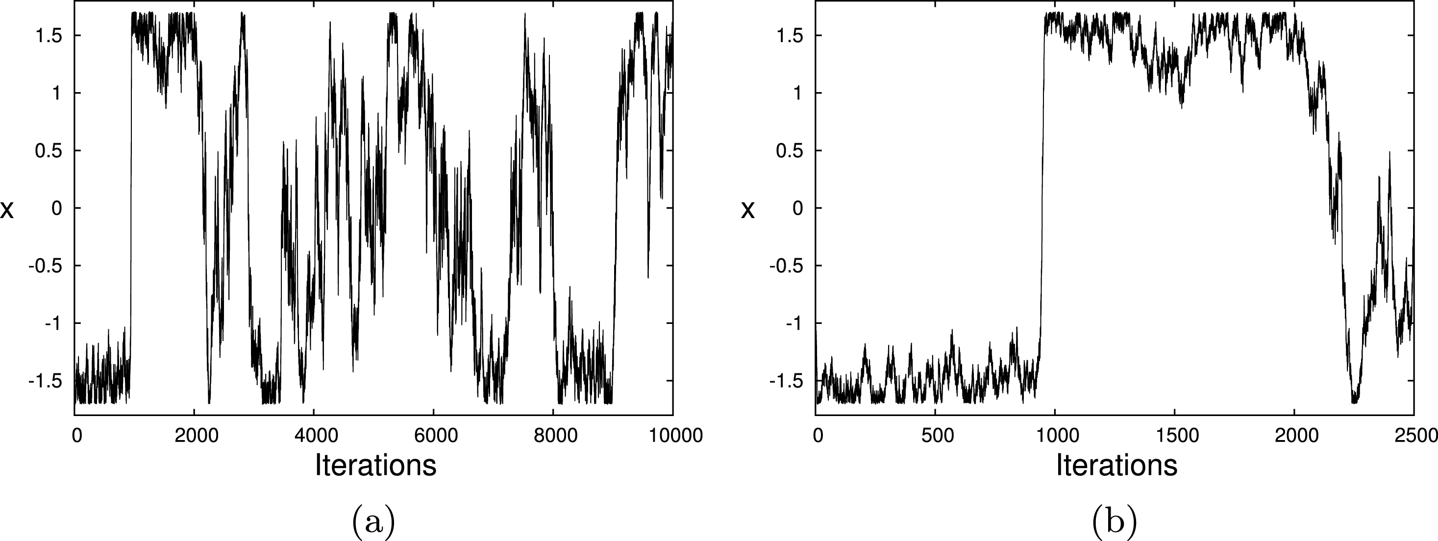
Average exit time from the left well as a function of the inverse
temperature  ${\it\beta}$, for the ABF process (squares) compared to the unbiased
overdamped Langevin dynamics (circles: see also
Figure 1.2(a)).
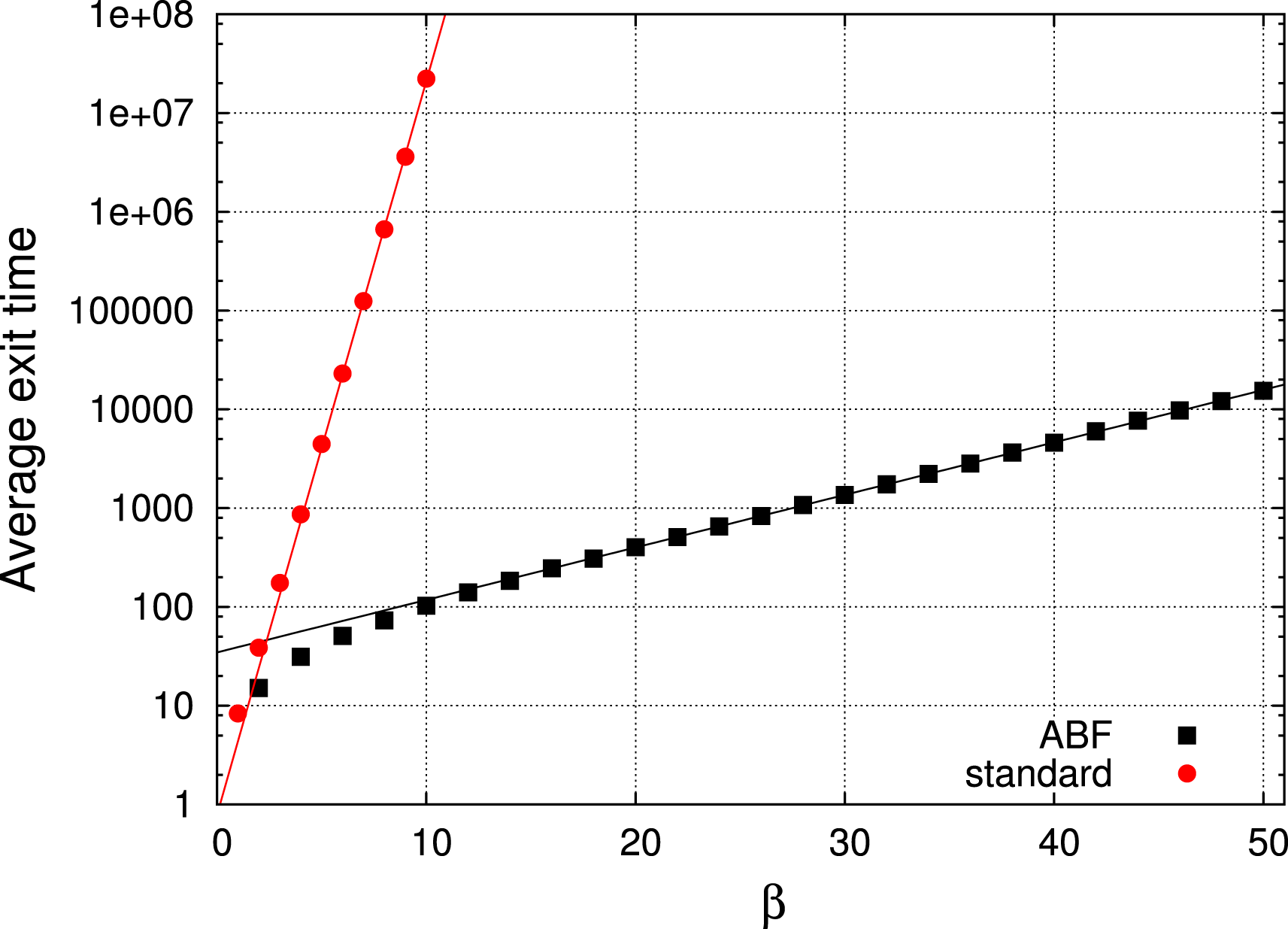
4.3 A convergence analysis using entropy techniques
In this section we present a typical example where the use of PDE techniques, and
more precisely entropy estimates and logarithmic Sobolev inequalities (see
Section 2.2.2), appear to be
very useful for understanding the efficiency of a numerical method, namely the
adaptive biasing force (ABF) method. For pedagogical purposes, the convergence result
is presented in a very simple setting (the two-dimensional case and  ${\it\xi}(x,y)=x$). Extensions are discussed in the next section.
4.3.1 The theoretical setting and the convergence result
Let us again consider the two-dimensional setting of Section 1.2, where  $q=(x,y)$ and
 ${\it\xi}(x,y)=x$. Let us assume in addition that
 $q$ lives in the space
 $\mathbb{T}\times \mathbb{R}$ (which simply means that
 $V:(x,y)\in \mathbb{R}^{2}\mapsto V(x,y)\in \mathbb{R}$ is
 $1$-periodic in the
 $x$-variable). We will comment on these assumptions below. In this
case, the mean force is given by
 $F^{\prime }(x)=\mathbb{E}_{{\it\nu}}(\partial _{x}V(q)|{\it\xi}(q)=x)$ (see (4.9)).
Thus, the free energy biased dynamics on
 $q_{t}=(x_{t},y_{t})\in \mathbb{T}\times \mathbb{R}$ is given by
 $$\begin{eqnarray}\displaystyle \text{d}x_{t} & = & \displaystyle -\partial _{x}V(x_{t},y_{t})\,\text{d}t+F^{\prime }(x_{t})\,\text{d}t+\sqrt{2{\it\beta}^{-1}}\,\text{d}W_{t}^{x},\end{eqnarray}$$
 $$\begin{eqnarray}\displaystyle \text{d}y_{t} & = & \displaystyle -\partial _{y}V(x_{t},y_{t})\,\text{d}t+\sqrt{2{\it\beta}^{-1}}\,\text{d}W_{t}^{y},\end{eqnarray}$$
 $$\begin{eqnarray}\displaystyle F^{\prime }(x) & = & \displaystyle \mathbb{E}_{{\it\nu}}(\partial _{x}V(q)|{\it\xi}(q)=x).\end{eqnarray}$$
 $q_{t}=(x_{t},y_{t})$ using the free energy biased potential
 $V(x,y)-F(x)$. Equation (4.17c) is the definition of the derivative of the
free energy. As explained above (see (4.14)), the ABF strategy is to replace the measure
 ${\it\nu}$ in this definition by the law at time
 $t$ of the pair
 $(x_{t},y_{t})$, which yields
 $$\begin{eqnarray}\displaystyle \text{d}x_{t} & = & \displaystyle -\partial _{x}V(x_{t},y_{t})\,\text{d}t+F_{t}^{\prime }(x_{t})\,\text{d}t+\sqrt{2{\it\beta}^{-1}}\,\text{d}W_{t}^{x},\end{eqnarray}$$
 $$\begin{eqnarray}\displaystyle \text{d}y_{t} & = & \displaystyle -\partial _{y}V(x_{t},y_{t})\,\text{d}t+\sqrt{2{\it\beta}^{-1}}\,\text{d}W_{t}^{y},\end{eqnarray}$$
 $$\begin{eqnarray}\displaystyle F_{t}^{\prime }(x) & = & \displaystyle \mathbb{E}(\partial _{x}V(x_{t},y_{t})|x_{t}=x).\end{eqnarray}$$
 $V(x,y)-F_{t}(x)$, then
 $F_{t}^{\prime }$ would be equal to
 $F^{\prime }$ (see (4.13)).
But the updating strategy is dynamic:
 $F_{t}$ always keeps on changing and it is therefore not obvious how the
system behaves in the transient phase of the dynamics (4.18). The objective of the
mathematical analysis is to be able to prove that
 $F_{t}^{\prime }$ indeed converges to
 $F^{\prime }$, and that, in addition, this convergence typically occurs on
much smaller time scales than the convergence to equilibrium for the original
simple overdamped Langevin dynamics:
 $$\begin{eqnarray}\text{d}q_{t}=-{\rm\nabla}V(q_{t})\,\text{d}t+\sqrt{2{\it\beta}^{-1}}\,\text{d}W_{t}.\end{eqnarray}$$
In order to study the rate of convergence to equilibrium, we will
actually analyse the long-time behaviour of the densityFootnote 11  ${\it\psi}(t,x,y)$ of the process
 $(x_{t},y_{t})$ solution to (4.18), namely the Fokker–Planck equation associated with (4.18):
 $$\begin{eqnarray}\displaystyle \partial _{t}{\it\psi} & = & \displaystyle \partial _{x}[(\partial _{x}V-F_{t}^{\prime }){\it\psi}]+{\it\beta}^{-1}\partial _{x,x}{\it\psi}\nonumber\\ \displaystyle & & \displaystyle \quad +\partial _{y}[(\partial _{y}V){\it\psi}]+{\it\beta}^{-1}\partial _{y,y}{\it\psi}\quad \text{for }(x,y)\in \mathbb{T}\times \mathbb{R},\end{eqnarray}$$
 $$\begin{eqnarray}\displaystyle F_{t}^{\prime }(x) & = & \displaystyle \frac{\int _{\mathbb{R}}\partial _{x}V(x,y){\it\psi}(t,x,y)\,\text{d}y}{\int _{\mathbb{R}}{\it\psi}(t,x,y)\,\text{d}y}\quad \text{for }x\in \mathbb{T}.\end{eqnarray}$$
 $t$ and
 $x\in \mathbb{T}$,
 ${\it\psi}(t,x,y)\,\text{d}y/\int _{\mathbb{R}}{\it\psi}(t,x,y)\,\text{d}y$ is indeed the conditional law at time
 $t$ of
 $(x_{t},y_{t})$ given that
 $x_{t}=x$. In the following, we will let
 ${\it\psi}^{{\it\xi}}$ denote the marginal of
 ${\it\psi}$ along
 ${\it\xi}$ (i.e. the density of
 $x_{t}$):
 $$\begin{eqnarray}{\it\psi}^{{\it\xi}}(t,x)=\int _{\mathbb{R}}{\it\psi}(t,x,y)\,\text{d}y.\end{eqnarray}$$
In contrast to the Fokker–Planck equation for simple overdamped Langevin dynamics (4.19), that is,
 $$\begin{eqnarray}\partial _{t}{\it\phi}=\text{div}({\rm\nabla}V{\it\phi})+{\it\beta}^{-1}{\rm\Delta}{\it\phi}\end{eqnarray}$$
(see (2.12)), the Fokker–Planck equation (4.20) is a non-linear parabolic equation. The non-linearity comes from the conditional expectation which appears in the drift term of the stochastic differential equation (4.18).
The following result is proved in Lelièvre, Rousset and Stoltz (Reference Lelièvre, Rousset and Stoltz2008) in a more general setting.
Theorem 4.6 (convergence of ABF).
Let us consider the ABF dynamics (4.18) on the domain  $\mathbb{T}\times \mathbb{R}$. Let us assume that
 $$\begin{eqnarray}\displaystyle & & \displaystyle \text{There exists }{\it\rho}>0\text{ such that all the conditional }\nonumber\\ \displaystyle & & \displaystyle \text{measures }{\it\nu}(\text{d}q|{\it\xi}(q)=x)\text{ satisfy LSI}({\it\rho})\end{eqnarray}$$
and that
 $$\begin{eqnarray}\text{The potential }V\text{ is such that }\Vert \partial _{x,y}V\Vert _{L^{\infty }(\mathbb{T}\times \mathbb{R})}<\infty .\end{eqnarray}$$
Let us assume in addition and (without loss of generality)
that  ${\it\rho}\neq 4{\it\pi}^{2}$ and that
 ${\it\psi}^{{\it\xi}}(0,\cdot )$ is a positive function such thatFootnote 12
 $\int _{\mathbb{T}}|\partial _{x}\ln ({\it\psi}^{{\it\xi}}(0,\cdot ))|^{2}{\it\psi}^{{\it\xi}}(0,\cdot )<\infty$. Then there exists a positive constant
 $C$ such that
 $$\begin{eqnarray}\sqrt{\int _{\mathbb{T}}|F_{t}^{\prime }-F^{\prime }|^{2}}\leqslant C\exp (-{\it\beta}^{-1}\min ({\it\rho},4{\it\pi}^{2})t),\quad \text{for all }t\geqslant 0.\end{eqnarray}$$
In our specific context, note that the conditional measure  ${\it\nu}(\text{d}q|{\it\xi}(q)=x)$ is simply the measure
 $$\begin{eqnarray}\frac{\exp (-{\it\beta}V(x,y))\,\text{d}y}{\int _{\mathbb{R}}\exp (-{\it\beta}V(x,y))\,\text{d}y}.\end{eqnarray}$$
Notice in addition that if  ${\it\rho}=4{\it\pi}^{2}$ in (4.21), one can use this result by replacing
 ${\it\rho}$ with any
 $\tilde{{\it\rho}}<{\it\rho}$, so that (4.23) holds in this case for any
 $\tilde{{\it\rho}}<4{\it\pi}^{2}$. Finally, we will show below (see (4.24)) that
 ${\it\psi}^{{\it\xi}}$ simply satisfies the heat equation on
 $\mathbb{T}$, so that the assumptions on
 ${\it\psi}^{{\it\xi}}(0,\cdot )$ are not too stringent: if they are not satisfied by
 ${\it\psi}^{{\it\xi}}(0,\cdot )$, one simply has to consider the problem on the time interval
 $[t_{0},+\infty )$ with initial condition
 ${\it\psi}^{{\it\xi}}(t_{0},\cdot )$, for a positive time
 $t_{0}$.
Let us comment on Theorem 4.6. This theorem shows that the free energy  $F_{t}$ indeed converges to
 $F$ (up to an irrelevant additive constant) with rate
 $$\begin{eqnarray}{\it\beta}^{-1}\min ({\it\rho},4{\it\pi}^{2}).\end{eqnarray}$$
As will be more clear below, the limiting parameter here is  ${\it\rho}$, the term
 $4{\it\pi}^{2}$ being only related to the rate of convergence to equilibrium of
a simple diffusion on the torus
 $\mathbb{T}$. Further, we will actually show that the law of
 $(x_{t},y_{t})$ (and not only
 $F_{t}$) converges to its equilibrium value at this rate (see (4.38) and the discussion below).
This rate of convergence for ABF has to be compared with (2.29), which shows that the original
simple overdamped Langevin dynamics (4.19) converges to equilibrium with rate
 $$\begin{eqnarray}{\it\beta}^{-1}R,\end{eqnarray}$$
where  $R$ is the logarithmic Sobolev constant of the measure
 ${\it\nu}$. In summary, by using ABF,
 $R$ has been replaced by
 ${\it\rho}$: the logarithmic Sobolev inequality constant of the measure
 ${\it\nu}$ has been replaced by the logarithmic Sobolev inequality constant
of the measures
 ${\it\nu}(\text{d}q|{\it\xi}(q)=x)$. If the function
 ${\it\xi}$ is indeed a good index of the metastable features of the
original dynamics, it is typically expected that
 ${\it\rho}\gg R$. This inequality is actually a way to quantify the somewhat
vague ideas that a good reaction coordinate
 ${\it\xi}$ should be such that ‘the metastability of the process
 $(q_{t})_{t\geqslant 0}$ is along
 ${\it\xi}$’ or that ‘the directions orthogonal to
 ${\it\xi}$ are fast variables’, so that equilibrium is quickly
reached along those directions. For example, in the two-dimensional examples of
Figure 1.1, the logarithmic
Sobolev constant of the measure
 ${\it\nu}$ is typically very small, while, for a fixed value of
 ${\it\xi}$ (where
 ${\it\xi}(x,y)=x$), the conditional measures
 ${\it\nu}(\text{d}q|{\it\xi}(q)=x)$ are gentle unimodal measures with much larger associated
logarithmic Sobolev constants. Unfortunately, logarithmic Sobolev constants are
very delicate to evaluate, and it thus seems very difficult to turn this measure
of the quality of
 ${\it\xi}$ into a numerical procedure to construct good reaction
coordinates. This result should thus be seen as a way to understand theoretically
the conditions under which an ABF strategy will be efficient, the measure of
efficiency being the rate of convergence to equilibrium.
4.3.2 Proof of Theorem 4.6
The proof of convergence is based on two ingredients: (i) the
observation that  ${\it\psi}^{{\it\xi}}(t,x)$ (which, we recall, is the density at time
 $t$ of
 $x_{t}$) satisfies the simple diffusion equation
 $$\begin{eqnarray}\partial _{t}{\it\psi}^{{\it\xi}}={\it\beta}^{-1}\partial _{x,x}{\it\psi}^{{\it\xi}}\text{ on }\mathbb{T},\end{eqnarray}$$
which is again a manifestation of the fact that, by using ABF, the
potential  $V$ is ‘flattened’ along the reaction
coordinate
 ${\it\xi}$ (see also equation (4.6)); (ii) entropy estimates in the vein of those explained
in Section 2.2.2, and a
two-scale decomposition of the entropy in the spirit of Otto and Reznikoff (Reference Otto and Reznikoff2007), Grunewald, Otto, Villani and
Westdickenberg (Reference Grunewald, Otto, Villani and Westdickenberg2009) and
Lelièvre (Reference Lelièvre2009). Let us now
present these ideas in detail.
The first ingredient of the proof is based on a simple computation, which consists
in looking at the evolution of the marginal of  ${\it\psi}$ along
 ${\it\xi}$, namely,
 $$\begin{eqnarray}{\it\psi}^{{\it\xi}}(t,x)=\int _{\mathbb{R}}{\it\psi}(t,x,y)\,\text{d}y.\end{eqnarray}$$
By direct integration in  $y$ of (4.20), we
obtain
 $$\begin{eqnarray}\displaystyle & & \displaystyle \partial _{t}{\it\psi}^{{\it\xi}}(t,x)\nonumber\\ \displaystyle & & \displaystyle \qquad =\partial _{x}\biggl(\int _{\mathbb{R}}\partial _{x}V(x,y){\it\psi}(t,x,y)\,\text{d}y-F_{t}^{\prime }(x){\it\psi}^{{\it\xi}}(t,x)\biggr)+{\it\beta}^{-1}\partial _{x,x}{\it\psi}^{{\it\xi}}(t,x)\nonumber\end{eqnarray}$$
which yields (4.24) since
 $$\begin{eqnarray}\int _{\mathbb{R}}\partial _{x}V(x,y){\it\psi}(t,x,y)\,\text{d}y-F_{t}^{\prime }(x){\it\psi}^{{\it\xi}}(t,x)=0,\end{eqnarray}$$
by the definition of  $F_{t}^{\prime }(x)$. This means that the law of
 $x_{t}$ satisfies a simple heat equation on
 $\mathbb{T}$, as for a simple Brownian motion on the torus.Footnote 13 This explains the interest of the ABF method: along
 ${\it\xi}$, the time marginal of the process evolves as if the potential
 $V$ were perfectly flat. The convergence to equilibrium of
 ${\it\psi}^{{\it\xi}}(t,x)$ is thus very easy to analyse, and in particular we have the
following convergence in terms of Fisher information, which will be useful later
(see Lelièvre et al. Reference Lelièvre, Rousset and Stoltz2008, Lemma 5.29 for a proof).
Lemma 4.7 (convergence of ${\it\psi}^{{\it\xi}}$).

Let  ${\it\varphi}$ be the solution of the heat equation on the torus
 $\mathbb{T}$,
 $$\begin{eqnarray}\partial _{t}{\it\varphi}={\it\beta}^{-1}\partial _{x,x}{\it\varphi}\;\text{on}\;\mathbb{T},\end{eqnarray}$$
with initial condition  ${\it\varphi}(0,\cdot )$ such that
 $$\begin{eqnarray}\int _{\mathbb{T}}{\it\varphi}(0,\cdot )=1,\quad {\it\varphi}(0,\cdot )\geqslant 0,\quad {\mathcal{I}}({\it\varphi}(0,\cdot )|{\it\varphi}_{\infty })<\infty ,\end{eqnarray}$$
where  ${\it\varphi}_{\infty }\equiv 1$ is the long-time limit of
 ${\it\varphi}$. Then,
 $\text{for all }t\geqslant 0$,
 $$\begin{eqnarray}{\mathcal{I}}({\it\varphi}(t,\cdot )\mid {\it\varphi}_{\infty })\leqslant {\mathcal{I}}({\it\varphi}(0,\cdot )\mid {\it\varphi}_{\infty })\exp (-{\it\beta}^{-1}8{\it\pi}^{2}t).\end{eqnarray}$$
We recall that
 $$\begin{eqnarray}{\mathcal{I}}({\it\varphi}(t,\cdot )\mid {\it\varphi}_{\infty })=\int _{\mathbb{T}}\biggl|\partial _{x}\ln \biggl(\displaystyle \frac{{\it\varphi}(t,x)}{{\it\varphi}_{\infty }(x)}\biggr)\biggr|^{2}{\it\varphi}(t,x)\,\text{d}x\end{eqnarray}$$
is the Fisher information of  ${\it\varphi}(t,x)\,\text{d}x$ with respect to
 ${\it\varphi}_{\infty }(x)\,\text{d}x$ (see (2.25)).
The rate of convergence to equilibrium for
 ${\it\psi}(t,x,y)$ is limited by the rate of convergence to equilibrium for
 ${\it\psi}^{{\it\xi}}(t,y)$: this explains why there is a
 $4{\it\pi}^{2}$ appearing in the right-hand side of (4.23). This
 $4{\it\pi}^{2}$ is simply the first non-zero eigenvalue of the Laplacian on the
torus
 $\mathbb{T}$, which determines the rate of convergence to equilibrium for the
heat equation (4.25) on
 $\mathbb{T}$.
To understand the convergence to equilibrium, it now remains to understand the
convergence of the conditional measures  ${\it\psi}(t,x,y)\,\text{d}y/{\it\psi}^{{\it\xi}}(t,x)$. We will use entropy techniques to study their long-time
behaviours (see Section 2.2.2). Here comes the second ingredient of the proof, namely a
decomposition of the entropy in terms of marginal and conditional measures, very
much inspired by Otto and Reznikoff (Reference Otto and Reznikoff2007)
and Grunewald et al. (Reference Grunewald, Otto, Villani and Westdickenberg2009). Let us explain this decomposition. We let
 ${\it\psi}_{\infty }$ denote the expected long-time limit of
 ${\it\psi}(t,x,y)$, defined by
 $$\begin{eqnarray}{\it\psi}_{\infty }(x,y)=Z^{-1}\exp (-{\it\beta}(V(x,y)-F(x)))\end{eqnarray}$$
where
 $$\begin{eqnarray}Z=\int _{\mathbb{T}^{2}}\exp (-{\it\beta}(V(x,y)-F(x)))\,\text{d}x\,\text{d}y.\end{eqnarray}$$
The marginal of  ${\it\psi}_{\infty }$ along
 ${\it\xi}$ is
 $$\begin{eqnarray}{\it\psi}_{\infty }^{{\it\xi}}(x)=Z^{-1}\int _{\mathbb{R}}\exp [-{\it\beta}(V(x,y)-F(x))]\,\text{d}y=1\end{eqnarray}$$
and the conditional measure of  ${\it\psi}_{\infty }(x,y)\,\text{d}x\,\text{d}y$ given
 ${\it\xi}(x,y)=x$ is
 $$\begin{eqnarray}\frac{{\it\psi}_{\infty }(x,y)\,\text{d}y}{\int _{\mathbb{R}}{\it\psi}_{\infty }(x,y)\,\text{d}y}={\it\nu}(\cdot |{\it\xi}(q)=x).\end{eqnarray}$$
Likewise, as explained above, the marginal of  ${\it\psi}$ along
 ${\it\xi}$ is
 $$\begin{eqnarray}{\it\psi}^{{\it\xi}}(t,x)=\int _{\mathbb{R}}{\it\psi}(t,x,y)\,\text{d}y,\end{eqnarray}$$
and the conditional measure of  ${\it\psi}(t,x,y)\,\text{d}x\,\text{d}y$ given that
 ${\it\xi}(x,y)=x$ is
 ${\it\psi}(t,x,y)\,\text{d}y/{\it\psi}^{{\it\xi}}(t,x)$. Let us now introduce the total entropy (see (2.24))
 $$\begin{eqnarray}E(t)={\mathcal{H}}({\it\psi}(t,\cdot )|{\it\psi}_{\infty }),\end{eqnarray}$$
the macroscopic entropy (namely the relative entropy of the marginal laws)
 $$\begin{eqnarray}E_{M}(t)={\mathcal{H}}({\it\psi}^{{\it\xi}}(t,\cdot )|{\it\psi}_{\infty }^{{\it\xi}}),\end{eqnarray}$$
and the microscopic entropy
 $$\begin{eqnarray}E_{m}(t)=\int _{\mathbb{T}}e_{m}(t,x){\it\psi}^{{\it\xi}}(t,x)\,\text{d}x,\end{eqnarray}$$
where  $e_{m}(t,x)$ is the relative entropy associated with the conditional
measures:
 $$\begin{eqnarray}e_{m}(t,x)={\mathcal{H}}\biggl(\displaystyle \frac{{\it\psi}(t,x,y)\,\text{d}y}{{\it\psi}^{{\it\xi}}(t,x)}\,\bigg|\,\frac{{\it\psi}_{\infty }(x,y)\,\text{d}y}{{\it\psi}_{\infty }^{{\it\xi}}(x)}\biggr).\end{eqnarray}$$
It is straightforward to check the following relation.
Lemma 4.8 (extensivity of entropy).
 $$\begin{eqnarray}E(t)=E_{M}(t)+E_{m}(t),\quad \text{for all }t\geqslant 0.\end{eqnarray}$$
In order to measure the convergence of  ${\it\psi}(t,\cdot )$ to
 ${\it\psi}_{\infty }$, we will study the rate of convergence to zero of
 $E$. We already know that
 $E_{M}(t)$ converges exponentially fast to zero, that is,
 $$\begin{eqnarray}E_{M}(t)\leqslant E_{M}(0)\exp (-{\it\beta}^{-1}8{\it\pi}^{2}t),\quad \text{for all }t\geqslant 0.\end{eqnarray}$$
since the logarithmic Sobolev constant of the uniform law on  $\mathbb{T}$ is
 $4{\it\pi}^{2}$ (see for example Bakry et al. Reference Bakry, Gentil and Ledoux2014, Proposition 5.7.5) and it
is therefore sufficient to understand the convergence of
 $E_{m}(t)$ to zero. The convergence (4.31) can also be seen as a consequence of
Lemma 4.7 since
 $$\begin{eqnarray}\displaystyle E_{M}(t)={\mathcal{H}}({\it\psi}(t,\cdot )|{\it\psi}_{\infty }) & = & \displaystyle {\it\beta}^{-1}\int _{t}^{\infty }{\mathcal{I}}({\it\psi}(t,\cdot )|{\it\psi}_{\infty })\,\text{d}t\nonumber\\ \displaystyle & {\leqslant} & \displaystyle \displaystyle \frac{1}{8{\it\pi}^{2}}{\mathcal{I}}({\it\psi}(t,\cdot )|{\it\psi}_{\infty })\nonumber\\ \displaystyle & = & \displaystyle -\displaystyle \frac{{\it\beta}}{8{\it\pi}^{2}}\displaystyle \frac{\text{d}E_{M}}{\text{d}t}(t).\nonumber\end{eqnarray}$$
The proof of Theorem 4.6 is then conducted as follows. Starting from (4.30), we haveFootnote 14
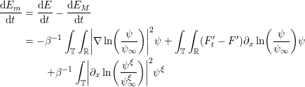 $$\begin{eqnarray}\displaystyle \frac{\text{d}E_{m}}{\text{d}t} & = & \displaystyle \frac{\text{d}E}{\text{d}t}-\frac{\text{d}E_{M}}{\text{d}t}\nonumber\\ \displaystyle & = & \displaystyle -{\it\beta}^{-1}\int _{\mathbb{T}}\int _{\mathbb{R}}\biggl|{\rm\nabla}\ln \biggl(\displaystyle \frac{{\it\psi}}{{\it\psi}_{\infty }}\biggr)\biggr|^{2}{\it\psi}+\int _{\mathbb{T}}\int _{\mathbb{R}}(F_{t}^{\prime }-F^{\prime })\partial _{x}\ln \biggl(\displaystyle \frac{{\it\psi}}{{\it\psi}_{\infty }}\biggr){\it\psi}\nonumber\\ \displaystyle & & \displaystyle \quad +{\it\beta}^{-1}\int _{\mathbb{T}}\biggl|\partial _{x}\ln \biggl(\frac{{\it\psi}^{{\it\xi}}}{{\it\psi}_{\infty }^{{\it\xi}}}\biggr)\biggr|^{2}{\it\psi}^{{\it\xi}}\end{eqnarray}$$
which is easily obtained after some integration by parts, using
the fact that  ${\it\psi}$ satisfies the following equation, which is equivalent to (4.20a):
 $$\begin{eqnarray}\partial _{t}{\it\psi}={\it\beta}^{-1}\text{div}\biggl({\it\psi}_{\infty }{\rm\nabla}\biggl(\displaystyle \frac{{\it\psi}}{{\it\psi}_{\infty }}\biggr)\biggr)+\partial _{x}((F^{\prime }-F_{t}^{\prime }){\it\psi}).\end{eqnarray}$$
We next rely on a very useful formula for  $F_{t}^{\prime }-F^{\prime }$.
Lemma 4.9. For all  $t\geqslant 0$, we have
 $$\begin{eqnarray}{\it\beta}(F_{t}^{\prime }-F^{\prime })=\int _{\mathbb{ T}}\partial _{x}\ln \biggl(\displaystyle \frac{{\it\psi}}{{\it\psi}_{\infty }}\biggr)\frac{{\it\psi}}{{\it\psi}^{{\it\xi}}}\,\text{d}y-\partial _{x}\ln \biggl(\displaystyle \frac{{\it\psi}^{{\it\xi}}}{{\it\psi}_{\infty }^{{\it\xi}}}\biggr).\end{eqnarray}$$
Proof. A simple computation gives (using the fact that  ${\it\psi}_{\infty }^{{\it\xi}}=1$)
 $$\begin{eqnarray}\displaystyle & & \displaystyle \int _{\mathbb{R}}\partial _{x}\ln \biggl(\displaystyle \frac{{\it\psi}}{{\it\psi}_{\infty }}\biggr)\frac{{\it\psi}}{{\it\psi}^{{\it\xi}}}\,\text{d}y-\partial _{x}\ln \biggl(\displaystyle \frac{{\it\psi}^{{\it\xi}}}{{\it\psi}_{\infty }^{{\it\xi}}}\biggr)\nonumber\\ \displaystyle & & \displaystyle \qquad =\int _{\mathbb{R}}\partial _{x}\ln {\it\psi}\frac{{\it\psi}}{{\it\psi}^{{\it\xi}}}\,\text{d}y-\int _{\mathbb{R}}\partial _{x}\ln {\it\psi}_{\infty }\frac{{\it\psi}}{{\it\psi}^{{\it\xi}}}\,\text{d}y-\partial _{x}\ln {\it\psi}^{{\it\xi}}\nonumber\\ \displaystyle & & \displaystyle \qquad =\int _{\mathbb{R}}\frac{\partial _{x}{\it\psi}}{{\it\psi}^{{\it\xi}}}\,\text{d}y+{\it\beta}\int _{\mathbb{R}}\partial _{x}(V-F)\frac{{\it\psi}}{{\it\psi}^{{\it\xi}}}\,\text{d}y-\partial _{x}\ln {\it\psi}^{{\it\xi}}\nonumber\\ \displaystyle & & \displaystyle \qquad ={\it\beta}(F_{t}^{\prime }-F^{\prime }),\nonumber\end{eqnarray}$$
where in the last line we used
 $$\begin{eqnarray}\partial _{x}\ln {\it\psi}^{{\it\xi}}=\frac{1}{{\it\psi}^{{\it\xi}}}\partial _{x}\int _{\mathbb{R}}{\it\psi}\,\text{d}y=\int _{\mathbb{R}}\frac{\partial _{x}{\it\psi}}{{\it\psi}^{{\it\xi}}}\,\text{d}y.\end{eqnarray}$$
This concludes the proof.
By using (4.33) in (4.32), we obtain
 $$\begin{eqnarray}\displaystyle & & \displaystyle \frac{\text{d}E_{m}}{\text{d}t}=-{\it\beta}^{-1}\int _{\mathbb{T}}\int _{\mathbb{R}}\biggl|\partial _{y}\ln \biggl(\frac{{\it\psi}}{{\it\psi}_{\infty }}\biggr)\biggr|^{2}{\it\psi}\nonumber\\ \displaystyle & & \displaystyle \qquad -{\it\beta}^{-1}\int _{\mathbb{T}}\int _{\mathbb{R}}\biggl|\partial _{x}\ln \biggl(\frac{{\it\psi}}{{\it\psi}_{\infty }}\biggr)\biggr|^{2}{\it\psi}+{\it\beta}^{-1}\int _{\mathbb{T}}\biggl(\int _{\mathbb{R}}\partial _{x}\ln \biggl(\displaystyle \frac{{\it\psi}}{{\it\psi}_{\infty }}\biggr){\it\psi}\,\text{d}y\biggr)^{2}\frac{1}{{\it\psi}^{{\it\xi}}}\,\text{d}x\nonumber\\ \displaystyle & & \displaystyle \qquad -{\it\beta}^{-1}\int _{\mathbb{T}}\int _{\mathbb{R}}\partial _{x}\ln \biggl(\displaystyle \frac{{\it\psi}^{{\it\xi}}}{{\it\psi}_{\infty }^{{\it\xi}}}\biggr)\partial _{x}\ln \biggl(\frac{{\it\psi}}{{\it\psi}_{\infty }}\biggr){\it\psi}+{\it\beta}^{-1}\int _{\mathbb{T}}\biggl|\partial _{x}\ln \biggl(\displaystyle \frac{{\it\psi}^{{\it\xi}}}{{\it\psi}_{\infty }^{{\it\xi}}}\biggr)\biggr|^{2}{\it\psi}^{{\it\xi}}.\nonumber\end{eqnarray}$$
Note that by the Cauchy–Schwarz inequality, the sum of the two terms on the second line above is non-positive. Therefore, again using (4.33),
 $$\begin{eqnarray}\displaystyle \frac{\text{d}E_{m}}{\text{d}t}\leqslant -{\it\beta}^{-1}\int _{\mathbb{T}}\int _{\mathbb{R}}\biggl|\partial _{y}\ln \biggl(\displaystyle \frac{{\it\psi}}{{\it\psi}_{\infty }}\biggr)\biggr|^{2}{\it\psi}-\int _{\mathbb{T}}\partial _{x}\ln \biggl(\displaystyle \frac{{\it\psi}^{{\it\xi}}}{{\it\psi}_{\infty }^{{\it\xi}}}\biggr){\it\psi}^{{\it\xi}}(F_{t}^{\prime }-F^{\prime }). & & \displaystyle\end{eqnarray}$$
Further, using assumption (4.21), we know that for any positive time  $t$, and for any
 $x\in \mathbb{T}$,
 $$\begin{eqnarray}{\mathcal{H}}\biggl(\displaystyle \frac{{\it\psi}(t,x,\cdot )}{{\it\psi}^{{\it\xi}}(t,x)}\Big|\frac{{\it\psi}_{\infty }(x,\cdot )}{{\it\psi}_{\infty }^{{\it\xi}}(x)}\biggr)\leqslant \frac{1}{2{\it\rho}}{\mathcal{I}}\biggl(\displaystyle \frac{{\it\psi}(t,x,\cdot )}{{\it\psi}^{{\it\xi}}(t,x)}\Big|\frac{{\it\psi}_{\infty }(x,\cdot )}{{\it\psi}_{\infty }^{{\it\xi}}(x)}\biggr),\end{eqnarray}$$
which is given more explicitly by
 $$\begin{eqnarray}\displaystyle e_{m}(t,x) & {\leqslant}\frac{1}{2{\it\rho}}\int _{\mathbb{R}}\biggl|\partial _{y}\ln \biggl(\frac{{\it\psi}/{\it\psi}^{{\it\xi}}}{{\it\psi}_{\infty }/{\it\psi}_{\infty }^{{\it\xi}}}\biggr)\biggr|^{2}\frac{{\it\psi}}{{\it\psi}^{{\it\xi}}}\,\text{d}y=\frac{1}{2{\it\rho}}\int _{\mathbb{R}}\biggl|\partial _{y}\ln \biggl(\displaystyle \frac{{\it\psi}}{{\it\psi}_{\infty }}\biggr)\biggr|^{2}\frac{{\it\psi}}{{\it\psi}^{{\it\xi}}}\,\text{d}y & \displaystyle \nonumber\end{eqnarray}$$
since  ${\it\psi}^{{\it\xi}}$ and
 ${\it\psi}_{\infty }^{{\it\xi}}$ do not depend on
 $y$. Therefore
 $$\begin{eqnarray}\displaystyle E_{m}(t)=\int _{\mathbb{T}}e_{m}(t,x){\it\psi}^{{\it\xi}}(t,x)\,\text{d}x\leqslant \frac{1}{2{\it\rho}}\int _{\mathbb{T}}\int _{\mathbb{R}}\biggl|\partial _{y}\ln \biggl(\displaystyle \frac{{\it\psi}}{{\it\psi}_{\infty }}\biggr)\biggr|^{2}{\it\psi}. & & \displaystyle \nonumber\end{eqnarray}$$
By using this in (4.34), we thus obtain
 $$\begin{eqnarray}\displaystyle \frac{\text{d}E_{m}}{\text{d}t}\leqslant -2{\it\beta}^{-1}{\it\rho}E_{m}-\int _{\mathbb{T}}\partial _{x}\ln \biggl(\displaystyle \frac{{\it\psi}^{{\it\xi}}}{{\it\psi}_{\infty }^{{\it\xi}}}\biggr){\it\psi}^{{\it\xi}}(F_{t}^{\prime }-F^{\prime }). & & \displaystyle\end{eqnarray}$$
To continue, we now need an upper bound on  $F_{t}^{\prime }-F^{\prime }$ in terms of the ‘distance’ (in some sense)
between the two conditional measures
 $$\begin{eqnarray}{\it\psi}(t,x,y)\,\text{d}y/{\it\psi}^{{\it\xi}}(t,x)\quad \text{and}\quad {\it\psi}_{\infty }(x,y)\,\text{d}y/{\it\psi}_{\infty }^{{\it\xi}}(x).\end{eqnarray}$$
It seems natural that such an estimate holds since
 $$\begin{eqnarray}F_{t}^{\prime }(x)-F^{\prime }(x)=\int _{\mathbb{ R}}\partial _{x}V(x,y)\frac{{\it\psi}(t,x,y)\,\text{d}y}{{\it\psi}^{{\it\xi}}(t,x)}-\int _{\mathbb{R}}\partial _{x}V(x,y)\frac{{\it\psi}_{\infty }(x,y)\,\text{d}y}{{\it\psi}_{\infty }^{{\it\xi}}(x)}\end{eqnarray}$$
is the difference between the averages of the same function ( $\partial _{x}V$) with respect to the two conditional measures. It is the purpose
of the next lemma (which is probably the most technical part of the proof) to
obtain such an estimate, the ‘distance’ being measured in
terms of relative entropy.
Lemma 4.10. Suppose assumptions (4.21) and (4.22) are satisfied. Then, for all  $t\geqslant 0$ and for all
 $x\in \mathbb{T}$,
 $$\begin{eqnarray}|F_{t}^{\prime }(x)-F^{\prime }(x)|\leqslant \Vert \partial _{x,y}V\Vert _{L^{\infty }}\sqrt{\frac{2}{{\it\rho}}e_{m}(t,x)},\end{eqnarray}$$
where  $e_{m}$ is defined by (4.29).
Proof. The proof uses the Talagrand inequality, which relates the Wasserstein distance and the relative entropy between two probability measures. Let us first recall the Wasserstein distance and the Talagrand inequality.
Let us introduce the set of coupling measures  ${\rm\Pi}({\it\nu}_{t,x},{\it\nu}_{\infty ,x})$, where, for ease of notation, we let
 $$\begin{eqnarray}{\it\nu}_{t,x}(\text{d}y)={\it\psi}(t,x,y)\,\text{d}y/{\it\psi}^{{\it\xi}}(t,x),\quad {\it\nu}_{\infty ,x}(\text{d}y)={\it\psi}_{\infty }(x,y)\,\text{d}y/{\it\psi}_{\infty }^{{\it\xi}}(x),\end{eqnarray}$$
respectively, denote the conditional measures of
 $$\begin{eqnarray}{\it\psi}(t,x,y)\,\text{d}x\,\text{d}y,\quad {\it\psi}_{\infty }(x,y)\,\text{d}x\,\text{d}y\end{eqnarray}$$
given that  ${\it\xi}(x,y)=x$. By definition of
 ${\rm\Pi}({\it\nu}_{t,x},{\it\nu}_{\infty ,x})$, the measures
 ${\it\pi}\in {\rm\Pi}({\it\nu}_{t,x},{\it\nu}_{\infty ,x})$ are probability measures over
 $\mathbb{R}\times \mathbb{R}$ such that, for any
 $C^{\infty }$ and compactly supported test function
 ${\it\varphi}:\mathbb{R}\rightarrow \mathbb{R}$,
 $$\begin{eqnarray}\int _{\mathbb{R}\times \mathbb{R}}{\it\varphi}(y_{1}){\it\pi}(\text{d}y_{1},\,\text{d}y_{2})=\int _{\mathbb{R}}{\it\varphi}(y_{1}){\it\nu}_{t,x}(\text{d}y_{1})\end{eqnarray}$$
and
 $$\begin{eqnarray}\int _{\mathbb{R}\times \mathbb{R}}{\it\varphi}(y_{2}){\it\pi}(\text{d}y_{1},\,\text{d}y_{2})=\int _{\mathbb{R}}{\it\varphi}(y_{2}){\it\nu}_{\infty ,x}(\text{d}y_{2}).\end{eqnarray}$$
In other words, the marginal of  ${\it\pi}\in {\rm\Pi}({\it\nu}_{t,x},{\it\nu}_{\infty ,x})$ on the first (resp. the second) variable is
 ${\it\nu}_{t,x}$ (resp.
 ${\it\nu}_{\infty ,x}$). Now, the Wasserstein distance between
 ${\it\nu}_{t,x}$ and
 ${\it\nu}_{\infty ,x}$ is denoted by
 ${\mathcal{W}}({\it\nu}_{t,x},{\it\nu}_{\infty ,x})$ where, for any measures
 ${\it\pi}_{1}$ and
 ${\it\pi}_{2}$ on
 $\mathbb{R}^{d}$, the Wasserstein distance between
 ${\it\pi}_{1}$ and
 ${\it\pi}_{2}$ is
 $$\begin{eqnarray}{\mathcal{W}}({\it\pi}_{1},{\it\pi}_{2})=\sqrt{\inf _{{\it\pi}\in {\rm\Pi}({\it\pi}_{1},{\it\pi}_{2})}\int _{\mathbb{R}\times \mathbb{R}}|y_{1}-y_{2}|^{2}{\it\pi}(\text{d}y_{1},\text{d}y_{2})}.\end{eqnarray}$$
The Wasserstein distance appears very naturally when estimating the
difference  $F_{t}^{\prime }-F^{\prime }$. Indeed, for any coupling measure
 ${\it\pi}\in {\rm\Pi}({\it\nu}_{t,x},{\it\mu}_{\infty ,x})$, we have
 $$\begin{eqnarray}\displaystyle |F_{t}^{\prime }(x)-F^{\prime }(x)| & = & \displaystyle \biggl|\int _{\mathbb{R}\times \mathbb{R}}(\partial _{x}V(x,y)-\partial _{x}V(x,y^{\prime })){\it\pi}(\text{d}y,\text{d}y^{\prime })\biggr|\nonumber\\ \displaystyle & {\leqslant} & \displaystyle \Vert \partial _{x,y}V\Vert _{L^{\infty }}\int _{\mathbb{R}\times \mathbb{R}}|y-y^{\prime }|{\it\pi}(\text{d}y,\text{d}y^{\prime })\nonumber\\ \displaystyle & {\leqslant} & \displaystyle \Vert \partial _{x,y}V\Vert _{L^{\infty }}\sqrt{\int _{\mathbb{R}\times \mathbb{R}}|y-y^{\prime }|^{2}{\it\pi}(\text{d}y,\text{d}y^{\prime })}.\nonumber\end{eqnarray}$$
Now taking the infimum over all  ${\it\pi}\in {\rm\Pi}({\it\nu}_{t,x},{\it\nu}_{\infty ,x})$, we get
 $$\begin{eqnarray}|F_{t}^{\prime }(x)-F^{\prime }(x)|\leqslant \Vert \partial _{x,y}V\Vert _{L^{\infty }}W({\it\nu}_{t,x},{\it\nu}_{\infty ,x}).\end{eqnarray}$$
This is where the assumption (4.22) is needed.
Now, in (4.35), it is not
the Wasserstein distance between  ${\it\nu}_{t,x}$ and
 ${\it\nu}_{\infty ,x}$ which appears, but the relative entropy since in view
of (4.28),
 $$\begin{eqnarray}E_{m}=\int {\mathcal{H}}({\it\nu}_{t,x}|{\it\nu}_{\infty ,x}){\it\psi}^{{\it\xi}}(t,x)\,\text{d}x.\end{eqnarray}$$
The Talagrand inequality is exactly what we need since it relates the Wasserstein distance to the relative entropy between two measures. Bobkov and Götze (Reference Bobkov and Götze1999) and Otto and Villani (Reference Otto and Villani2000) have proved the following result (though in a more general setting).
Lemma 4.11 (Talagrand inequality).
Let  ${\it\pi}_{2}$ be a probability measure on
 $\mathbb{R}^{d}$ which satisfies
 $\text{LSI}({\it\rho})$. Then, for all probability measures
 ${\it\pi}_{1}$ on
 $\mathbb{R}^{d}$,
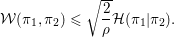 $$\begin{eqnarray}{\mathcal{W}}({\it\pi}_{1},{\it\pi}_{2})\leqslant \sqrt{\frac{2}{{\it\rho}}}{\mathcal{H}}({\it\pi}_{1}|{\it\pi}_{2}).\end{eqnarray}$$
Using this result and Assumption (4.21), which exactly states that  ${\it\nu}_{\infty ,x}={\it\nu}(\text{d}q|{\it\xi}(q)=x)$ satisfies LSI(
 ${\it\rho}$), we thus have
 $$\begin{eqnarray}{\mathcal{W}}({\it\nu}_{t,x},{\it\nu}_{\infty ,x})\leqslant \sqrt{\frac{2}{{\it\rho}}}{\mathcal{H}}({\it\nu}_{t,x}|{\it\nu}_{\infty ,x}),\quad \text{for all }t\geqslant 0.\end{eqnarray}$$
By using this inequality in (4.37), we thus obtain (4.36). This concludes the proof of Lemma 4.10.
Using (4.36) in (4.35), we obtain, using Cauchy–Schwarz,
 $$\begin{eqnarray}\displaystyle \frac{\text{d}E_{m}}{\text{d}t} & {\leqslant} & \displaystyle -2{\it\beta}^{-1}{\it\rho}E_{m}+\sqrt{\int _{\mathbb{T}}{\it\psi}^{{\it\xi}}|F_{t}^{\prime }-F^{\prime }|^{2}}\sqrt{\int _{\mathbb{T}}| \partial _{x}\ln (\displaystyle \frac{{\it\psi}^{{\it\xi}}}{{\it\psi}_{\infty }^{{\it\xi}}}\biggr)\biggr|^{2}{\it\psi}^{{\it\xi}}}\nonumber\\ \displaystyle & {\leqslant} & \displaystyle -2{\it\beta}^{-1}{\it\rho}E_{m}+\Vert \partial _{x,y}V\Vert _{L^{\infty }}\sqrt{\frac{2}{{\it\rho}}}\sqrt{E_{m}}\sqrt{{\mathcal{I}}({\it\psi}^{{\it\xi}}|{\it\psi}_{\infty }^{{\it\xi}})}.\nonumber\end{eqnarray}$$
By dividing by  $2\sqrt{E_{m}}$ and using the estimate (4.26) on
 ${\mathcal{I}}({\it\psi}^{{\it\xi}}|{\it\psi}_{\infty }^{{\it\xi}})$, we thus obtain
 $$\begin{eqnarray}\displaystyle \frac{\text{d}\sqrt{E_{m}}}{\text{d}t}\leqslant -{\it\beta}^{-1}{\it\rho}\sqrt{E_{m}}+\Vert \partial _{x,y}V\Vert _{L^{\infty }}\sqrt{\frac{1}{2{\it\rho}}{\mathcal{I}}({\it\psi}^{{\it\xi}}(0,\cdot )|{\it\psi}_{\infty }^{{\it\xi}})}\exp (-{\it\beta}^{-1}4{\it\pi}^{2}t). & & \displaystyle \nonumber\end{eqnarray}$$
Using the fact that  ${\it\rho}\neq 4{\it\pi}^{2}$, a Gronwall lemmaFootnote 15 then easily shows that there exists a constant
 $C$ such that, for all
 $t>0$,
 $$\begin{eqnarray}\sqrt{E_{m}(t)}\leqslant C\exp (-{\it\beta}^{-1}\min ({\it\rho},4{\it\pi}^{2})t).\end{eqnarray}$$
From this result, the extensivity of the entropy (4.30), and the convergence of the
marginals in  $x$ (4.31), one
immediately deduces that
 $\sqrt{E(t)}$ (and thus
 $\Vert {\it\psi}(t,\cdot )-{\it\psi}_{\infty }\Vert _{L^{1}(\mathbb{T}\times \mathbb{R})}$ by the Csiszár–Kullback inequality (2.27)) converges exponentially fast
to zero with rate
 ${\it\beta}^{-1}\min ({\it\rho},4{\it\pi}^{2})$.
To deduce from these results the convergence of
 $$\begin{eqnarray}\sqrt{\int _{\mathbb{T}}|F_{t}^{\prime }-F^{\prime }|^{2}}\end{eqnarray}$$
exponentially fast with the same rate, one simply uses the fact that
 $$\begin{eqnarray}\displaystyle \sqrt{\int _{\mathbb{T}}|F_{t}^{\prime }-F^{\prime }|^{2}}\leqslant C\sqrt{\int _{\mathbb{T}}|F_{t}^{\prime }-F^{\prime }|^{2}{\it\psi}^{{\it\xi}}}\leqslant C\sqrt{E_{m}(t)}. & & \displaystyle \nonumber\end{eqnarray}$$
The first inequality is a consequence of the fact that  ${\it\psi}^{{\it\xi}}(0,\cdot )$ is assumed to be positive and
 ${\it\psi}^{{\it\xi}}$ satisfies the heat equation on
 $\mathbb{T}$, so that
 ${\it\psi}^{{\it\xi}}$ is bounded from below by a positive constant. The second
inequality is a consequence of (4.36). This concludes the proof of Theorem 4.6.
4.4 Extensions and related works
4.4.1 Extensions of Theorem 4.6
Let us make a few comments on the specific setting in which we presented the
convergence result of Theorem 4.6. First, we assumed that the  $x$-variable lives in the torus in order for
 ${\it\xi}$ to be with values in a compact domain, so that the free energy
biased Boltzmann–Gibbs measure with density
 $\exp (-{\it\beta}(V-F\circ {\it\xi}))$ can be normalized. The fact that
 $\int \exp (-{\it\beta}(V-F\circ {\it\xi}))<\infty$ is necessary for the dynamics to actually have a stationary
state and this has already been discussed above (see (4.6)). In practice, if
 ${\it\xi}$ does not take values in a compact domain, the classical
technique is to apply the bias only over a compact domain, by using a restraining
potential
 ${\mathcal{W}}\circ {\it\xi}$ (see Lelièvre et al. Reference Lelièvre, Rousset and Stoltz2008, Alrachid and Lelièvre
Reference Alrachid and Lelièvre2015 for more details). Second, we
assumed that
 ${\it\xi}$ is a linear function of
 $q$. Let us consider the case of more general reaction coordinates
 ${\it\xi}:\mathbb{R}^{d}\rightarrow \mathbb{R}$ (we consider one-dimensional
 ${\it\xi}$ for simplicity). For general reaction coordinates, one in fact
has to slightly modify the ABF dynamics (4.18) by terms which depend on
 $|{\rm\nabla}{\it\xi}|$ in order to recover the results of Theorem 4.6 (see Lelièvre
et al. Reference Lelièvre, Rousset and Stoltz2008, equation (10)). These
modifications are only necessary for theoretical purposes: they are not used by
practitioners. However, from a theoretical viewpoint, without these additional
terms we are only able to prove a weaker result (see Lelièvre
et al. Reference Lelièvre, Rousset and Stoltz2008, Section 2.3). With these
additional terms, the results of Theorem 4.6 can be proved by rewriting (4.22) as
 $$\begin{eqnarray}\Vert {\rm\nabla}_{{\rm\Sigma}({\it\xi}(q))}f(q)\Vert _{L^{\infty }}<\infty\end{eqnarray}$$
(where  ${\rm\nabla}_{{\rm\Sigma}(z)}$ denotes the surface gradient in
 ${\rm\Sigma}(z)$ and
 $f$ is the local mean force: see (4.12)) and by assuming in addition
that there exists
 $m<\infty$ such that
 $$\begin{eqnarray}0<|{\rm\nabla}{\it\xi}(q)|\leqslant m,\quad \text{for all }q\in \mathbb{R}^{d}.\end{eqnarray}$$
Further, assumption (4.21) can
be somewhat weakened. Lelièvre and Minoukadeh (Reference Lelièvre and Minoukadeh2011) consider the situation when two channels link
metastable states, so that the assumption (4.21) is only satisfied on some bounded sub-interval of the
range of  ${\it\xi}$. In this situation, it can be shown that if the free energy
profile does not differ too much in each channel, then a similar convergence
result can be obtained.
Finally, Alrachid and Lelièvre (Reference Alrachid and Lelièvre2015) have proved the convergence of a variant of the ABF method, where the biasing force is projected onto a gradient field (which makes sense since the expected limit, the mean force, is indeed a gradient).
4.4.2 Related works
The pair of assumptions (4.21)
and (4.22) seem to be very
useful in other contexts. In Otto and Reznikoff (Reference Otto and Reznikoff2007) and Lelièvre (Reference Lelièvre2009), it appears as a set of assumptions in order to prove that a
logarithmic Sobolev inequality can be derived for a measure  ${\it\mu}$ if, for a given function
 ${\it\xi}$, it holds on the marginal probability measure
 $({\it\xi}\ast {\it\mu})(\text{d}q)$, on the conditional probability measures
 ${\it\mu}(\text{d}q|{\it\xi}(q)=z)$ (which corresponds to (4.21)) and if a so-called bounded coupling assumption of
the form (4.39) holds.
This set of assumptions also naturally appears in order to measure the error of a
coarse-graining technique, which yields an effective Markov dynamics which
approximates the dynamics of  $({\it\xi}(q_{t}))_{t\geqslant 0}$. The aim is thus to reduce the dimension of the original problem
by deriving an effective dynamics on the reaction coordinate. This is closely
related to the question of the relevance of the free energy to approximate
dynamical quantities such as transition times (and not only to compute
thermodynamic quantities). We refer to Legoll and Lelièvre (Reference Legoll and Lelièvre2010) for more results along these lines.
Similar assumptions are also used for Markov chains (in a discrete setting); see for example Madras and Randall (Reference Madras and Randall2002) and Jerrum, Son, Tetali and Vigoda (Reference Jerrum, Son, Tetali and Vigoda2004).
4.4.3 Open problems
Among the open problems related to free energy adaptive biasing techniques, the extension of the efficiency analysis to Langevin dynamics (as opposed to overdamped Langevin dynamics) remains to be done. As already explained in Section 2, the entropy technique does not apply to Langevin dynamics because of the lack of ellipticity. Hypocoercivity is then a good way to study the long-time behaviour of Langevin dynamics, and it would be interesting to extend the standard results on linear Langevin dynamics presented in Section 2.3 to the non-linear setting of adaptive biasing methods.
Let us also mention that we lack a good understanding of the efficiency of free energy adaptive techniques when time averages are used (instead of averages over multiple replicas) to compute the biasing force. We refer to Fort et al. Reference Fort, Jourdain, Kuhn, Lelièvre and Stoltz2015a, Reference Fort, Jourdain, Lelièvre and Stoltz2015b for convergence results for the Wang–Landau and self-healing umbrella sampling algorithms, and to Fort et al. (Reference Fort, Jourdain, Kuhn, Lelièvre and Stoltz2014) for a preliminary study of the efficiency of the Wang–Landau dynamics. See also Benaïm and Bréhier (Reference Benaïm and Bréhier2016) for recent results on ABP methods.
4.5 Other free energy computation techniques
In this section we have focused on adaptive importance sampling techniques for calculations of free energy differences. As mentioned above, such computations are actually the aim of many molecular dynamics simulations today (see Chipot and Pohorille Reference Chipot and Pohorille2007), and many techniques have been proposed to this end. We refer to Lelièvre et al. (Reference Lelièvre, Rousset and Stoltz2010) for an extensive presentation of such techniques. In this article we focus on adaptive importance sampling techniques, since their analysis typically relies on partial differential equation techniques. In practice, adaptive importance sampling approaches are very popular since they do not require many tuning parameters, and they appear to be rather efficient for a large class of systems. However, let us mention here the three other main classes of techniques for free energy calculations, aside from adaptive importance sampling methods.
Thermodynamic integration (Kirkwood Reference Kirkwood1935, Carter, Ciccotti, Hynes and Kapral Reference Carter, Ciccotti, Hynes and Kapral1989) consists in computing the free energy derivative, and then
integrating this derivative to obtain free energy differences. It is based on the
formula (4.10). Let us consider the
case of a one-dimensional reaction coordinate for simplicity (the generalization to  $m>1$ is straightforward). The principle is to compute
 $F^{\prime }(z_{i})$ at some points
 $(z_{1},\ldots ,z_{k})$ and then to use a numerical quadrature to approximate
 $F(z_{k})-F(z_{1})=\int _{z_{1}}^{z_{k}}F^{\prime }(z)\,\text{d}z$ by a weighted sum over the values
 $F^{\prime }(z_{i})$. This requires us to sample the conditional probability measures
 ${\it\nu}(\text{d}q|{\it\xi}(q)=z_{i})$, which can be done using Langevin or overdamped Langevin dynamics
projected onto the submanifold
 ${\rm\Sigma}(z_{i})$. We refer to Carter et al. (Reference Carter, Ciccotti, Hynes and Kapral1989), Ciccotti, Lelièvre and
Vanden-Eijnden (Reference Ciccotti, Lelièvre and Vanden-Eijnden2008) and Lelièvre,
Rousset and Stoltz (Reference Lelièvre, Rousset and Stoltz2012) for more details of
the sampling of such conditional measures, and to Lelièvre
et al. (Reference Lelièvre, Rousset and Stoltz2010,
Chapter 3) for a general presentation of thermodynamic integration
methods. Let us mention that the sampling of measures supported on submanifolds (such
as the conditional measures
 ${\it\nu}(\text{d}q|{\it\xi}(q)=z_{i})$) is actually a very important subject in practice. Apart from
thermodynamic integration, this question naturally appears when considering molecular
systems with constraints: for example, a covalent bond is sometimes modelled using a
fixed bond length instead of a stiff potential, which can be useful in diminishing
the stability constraint on the time step (see Remark 3.6). In such cases, the canonical
measure is defined on a submanifold of
 $\mathbb{R}^{3N}$ or
 $(L\mathbb{T})^{3N}$, and the differential operators associated with the ergodic
stochastic processes are differential operators on manifolds. For more details on
sampling methods with constraints, we refer to Lelièvre
et al. (Reference Lelièvre, Rousset and Stoltz2012).
Another free energy calculation method consists in using statistical approaches to
estimate directly the marginal density  $\exp (-{\it\beta}F(z))$. Examples include the free energy perturbation
method introduced in Zwanzig (Reference Zwanzig1954),
and histogram methods, such as the MBAR method (Shirts and Chodera
Reference Shirts and Chodera2008). We refer to Lelièvre
et al. (Reference Lelièvre, Rousset and Stoltz2010,
Sections 2.4 and 2.5) for more details and references.
A more recent class of methods relies on dynamics with an imposed schedule for the reaction coordinate. These technique therefore use non-equilibrium dynamics. With suitable exponential reweighting, however, equilibrium properties (such as free energy differences) can be recovered from the non-equilibrium trajectories: see Jarzynski (Reference Jarzynski1997). This is explained in Proposition 6.2 below in a slightly different setting (the so-called alchemical setting); see also Lelièvre et al. (Reference Lelièvre, Rousset and Stoltz2010, Chapter 4).
5 Non-equilibrium systems and transport coefficients
In this section we discuss how to compute transport coefficients such as the mobility, the thermal conductivity or the shear viscosity. At the macroscopic level, transport coefficients relate an external forcing acting on the system (e.g. electric field, temperature gradient, velocity field) to an average response expressed through some steady-state flux (i.e., of charged particles, energy, momentum). At the microscopic level, this is modelled by systems in a stationary state, evolving according to perturbations of equilibrium dynamics. Here we consider two paradigmatic situations.
(1) Langevin dynamics perturbed by a constant force term:
where(5.1a)$$\begin{eqnarray}\displaystyle \text{d}q_{t} & = & \displaystyle M^{-1}p_{t}\,\text{d}t,\end{eqnarray}$$(5.1b)$$\begin{eqnarray}\displaystyle \text{d}p_{t} & = & \displaystyle (-{\rm\nabla}V(q_{t})+{\it\eta}F)\,\text{d}t-{\it\gamma}M^{-1}p_{t}\,\text{d}t+\sqrt{\frac{2{\it\gamma}}{{\it\beta}}}\,\text{d}W_{t},\end{eqnarray}$$$(q_{t},p_{t})\in {\mathcal{E}}=\mathbb{T}^{d}\times \mathbb{R}^{d}$, $F\in \mathbb{R}^{d}$, with $|F|=1$ a given direction, and $V$ a $C^{\infty }$ periodic potential. The parameter ${\it\eta}\in \mathbb{R}$ determines the strength of the external forcing. A non-zero
velocity in the direction $F$ is expected in the steady state due to the external force $F$. Let us emphasize that $F$ does not derive from the gradient of a periodic function: it
indeed holds that $F=-{\rm\nabla}W_{F}(q)$ with $W_{F}(q)=-F^{T}q$, but the function $W_{F}$ is not periodic. It is precisely because the perturbation is
not of gradient type that some particle flux can appear in the steady
state.(2) Langevin dynamics with modified fluctuation:
where the temperature(5.2a)$$\begin{eqnarray}\displaystyle \text{d}q_{t} & = & \displaystyle M^{-1}p_{t}\,\text{d}t,\end{eqnarray}$$(5.2b)$$\begin{eqnarray}\displaystyle \text{d}p_{t} & = & \displaystyle -{\rm\nabla}V(q_{t})\,\text{d}t-{\it\gamma}M^{-1}p_{t}\,\text{d}t+\sqrt{2{\it\gamma}T_{{\it\eta}}(q)}\,\text{d}W_{t},\end{eqnarray}$$$T_{{\it\eta}}:{\mathcal{D}}\rightarrow \mathbb{R}_{+}$ is a non-negative $C^{\infty }$ function, of the form for some$$\begin{eqnarray}T_{{\it\eta}}(q)=T_{\text{ref}}+{\it\eta}\widetilde{T}(q)\end{eqnarray}$$$C^{\infty }$ function $\widetilde{T}$ and a given reference temperature $T_{\text{ref}}>0$. In order for $T_{{\it\eta}}$ to remain non-negative, the parameter ${\it\eta}\in \mathbb{R}$ should be sufficiently small. Typically, $\widetilde{T}$ is constant and positive on a subdomain ${\mathcal{D}}_{+}\subset {\mathcal{D}}$, and constant and negative on another subdomain ${\mathcal{D}}_{-}\subset {\mathcal{D}}$, with some $C^{\infty }$ transition between ${\mathcal{D}}_{+}$ and ${\mathcal{D}}_{-}$. Some energy flux is expected from the
‘hot’ part ${\mathcal{D}}_{+}$ of the system to the ‘cold’ one ${\mathcal{D}}_{-}$. The model (5.2) we consider here for pedagogical purposes is a
simplification of more realistic models of thermal transport such as heat
transport in one-dimensional chains; see the model presented in Olla and
Letizia (Reference Olla and Letizia2015), as well as the more
general review articles by Bonetto, Lebowitz and Rey-Bellet (Reference Bonetto, Lebowitz, Rey-Bellet and Fokas2000), Lepri, Livi and Politi (Reference Lepri, Livi and Politi2003) and Dhar (Reference Dhar2008).










The two dynamics (5.1)
and (5.2) reduce to the
standard Langevin dynamics (1.9) when  ${\it\eta}=0$. Most of our analysis is illustrated with the
dynamics (5.1), but we
will occasionally refer to the dynamics (5.2) as well.
As discussed more precisely in Section 5.1, dynamics such as (5.1) and (5.2) model non-equilibrium systems since they are non reversible: the law of forward trajectories is different from the law of backward trajectories. From a physical point of view, the arrow of time can be read off the trajectories. We do not make a distinction here between non-reversible and non-equilibrium systems, although such a distinction is sometimes made in the physical literature; see for instance (Bertini et al. Reference Bertini, De Sole, Gabrielli, Jona-Lasinio and Landim2015) and references therein.
It is observed that, in general, the response of the system, as encoded by the
steady-state average of a physical observable (such as the velocity
for (5.1) or the energy
flux for (5.2)), is
proportional to the strength  ${\it\eta}$ of the forcing for small values of
 ${\it\eta}$. This corresponds to the so-called linear response regime. By
definition, transport coefficients are the proportionality constants relating the
response to the forcing. For (5.1),
the velocity of the particle in the direction of
 $F$ at stationary state is proportional to
 ${\it\eta}$, and the proportionality constant is called the mobility. For (5.2), the energy flux at stationary state
is proportional to
 ${\it\eta}$, and the proportionality constant is called the thermal conductivity.
It turns out that this linear response constant can in fact be rewritten as some
integrated correlation function for an equilibrium dynamics, a celebrated equality known
as the Green–Kubo formula (see Proposition 5.4 below).
We start with a general presentation of non-equilibrium dynamics in
Section 5.1, with some emphasis on
perturbations of equilibrium dynamics such as (5.1) and (5.2).
We next show in Section 5.2 how
first-order changes in average properties with respect to some forcing parameter (namely  ${\it\eta}$ in (5.1) and (5.2)) can be computed, and how these
quantities are related to transport coefficients. Error estimates on the computation of
transport coefficients are provided in Section 5.3. Finally, we discuss variance reduction techniques in
Section 5.4.
5.1 Definition of non-equilibrium dynamics
5.1.1 Abstract characterization of non-equilibrium dynamics
Consider a general stochastic dynamics such as (3.1):
 $$\begin{eqnarray}\text{d}x_{t}=b(x_{t})\,\text{d}t+{\it\sigma}(x_{t})\,\text{d}W_{t}.\end{eqnarray}$$
Recall that the existence and uniqueness of an invariant
probability measure  ${\it\pi}$ can be proved in such a general setting with the techniques
provided in Section 2.4, for
instance. From a mathematical viewpoint, equilibrium systems are characterized by
the self-adjointness of the generator
 ${\mathcal{L}}$ on the weighted Hilbert space
 $L^{2}({\it\pi})$:
 $$\begin{eqnarray}\int _{{\mathcal{X}}}({\mathcal{L}}f)\,g\,\text{d}{\it\pi}=\int _{{\mathcal{X}}}f\,({\mathcal{L}}g)\,\text{d}{\it\pi}.\end{eqnarray}$$
This expresses the reversibility of the dynamics with respect to
the invariant measure of the process. A more probabilistic reformulation of the
reversibility is as follows: when  $x_{0}\sim {\it\pi}$, the law of the forward paths
 $(x_{s})_{0\leqslant s\leqslant t}$ is the same as the law of the backward paths
 $(x_{t-s})_{0\leqslant s\leqslant t}$ (note that
 $x_{t}\sim {\it\pi}$ by the invariance of
 ${\it\pi}$). Therefore, the arrow of time cannot be read off the
trajectories.
In some cases, the reversibility property holds only up to a one-to-one
transformation preserving the invariant measure. For example, for Langevin
dynamics, reversibility is valid only upon momentum reversal  $S(q,p)=(q,-p)$:
 $$\begin{eqnarray}\int _{{\mathcal{X}}}({\mathcal{L}}f)\,g\,\text{d}{\it\pi}=\int _{{\mathcal{X}}}(f\circ S)\,({\mathcal{L}}(g\circ S))\,\text{d}{\it\pi};\end{eqnarray}$$
see Lelièvre et al. (Reference Lelièvre, Rousset and Stoltz2010, Section 2.2.3.1). At the
level of trajectories, this means that the law of the forward paths  $(q_{s},p_{s})_{0\leqslant s\leqslant t}$ is the same as the law of the paths
 $(q_{t-s},-p_{t-s})_{0\leqslant s\leqslant t}$.
In this work, we define non-equilibrium dynamics to be stochastic evolutions for which reversibility properties such as (5.3) no longer hold true. The non-reversibility can be quantified by the entropy production, for which fluctuation theorems hold (Gallavotti and Cohen Reference Gallavotti and Cohen1995, Kurchan Reference Kurchan1998, Lebowitz and Spohn Reference Lebowitz and Spohn1999).
5.1.2 Invariant measures
An important property of non-equilibrium systems is that their invariant measures
are in general not analytically known, in contrast to equilibrium dynamics. In
addition, the invariant measure depends non-trivially on the details of the
dynamics due to long-range correlations, which are generally present in
non-equilibrium systems (see for instance Derrida, Lebowitz and Speer Reference Derrida, Lebowitz and Speer2002). Let us make the latter statement
precise for overdamped Langevin dynamics on the compact configuration space  $\mathbb{T}=\mathbb{R}/\mathbb{Z}$, for a
 $C^{\infty }$ periodic potential
 $V$ and
 ${\it\beta}=1$. For the reversible dynamics
 $$\begin{eqnarray}\text{d}q_{t}=-V^{\prime }(q_{t})\,\text{d}t+\sqrt{2}\,\text{d}W_{t},\end{eqnarray}$$
the unique invariant probability measure is  $Z^{-1}\text{e}^{-V(q)}\,\text{d}q$, which depends only on the value of
 $V$ at the configuration
 $q$ of interest (apart from a global normalization constant). For
the perturbed dynamics
 $$\begin{eqnarray}\text{d}q_{t}=(-V^{\prime }(q_{t})+F)\,\text{d}t+\sqrt{2}\,\text{d}W_{t},\end{eqnarray}$$
where  $F\in \mathbb{R}$ is a constant force, it can be shown that there exists a unique
invariant probability measure
 ${\it\psi}_{F}(q)\,\text{d}q$. Indeed, the density
 ${\it\psi}_{F}$ satisfies the stationary Fokker–Planck equation
 $$\begin{eqnarray}\frac{\text{d}}{\text{d}q}\biggl((V^{\prime }-F){\it\psi}_{F}+\frac{\text{d}{\it\psi}_{F}}{\text{d}q}\biggr)=0,\end{eqnarray}$$
which can be solved as
 $$\begin{eqnarray}{\it\psi}_{F}(q)=Z_{F}^{-1}\int _{\mathbb{T}}\,\text{e}^{V(q+y)-V(q)-Fy}\,\text{d}y,\end{eqnarray}$$
with  $Z_{F}$ chosen such that
 $\int _{0}^{1}{\it\psi}_{F}=1$. It is clear from the expression of the invariant measure that,
when
 $F\neq 0$, the invariant measure depends on the values of
 $V$ everywhere.
Let us also check that the dynamics (5.5) is a non-equilibrium dynamics by checking that its generator is
not reversible on  $L^{2}({\it\psi}_{F})$. Since we do not need the precise expression of the invariant
measure, we generalize the dynamics in arbitrary dimension, and consider
 ${\mathcal{D}}=\mathbb{T}^{d}$. We first rewrite
 ${\it\psi}_{F}$ in exponential form as
 $$\begin{eqnarray}{\it\psi}_{F}(q)=\text{e}^{-U_{F}(q)},\end{eqnarray}$$
and introduce a stochastic dynamics with a general drift  $b(q)$:
 $$\begin{eqnarray}\text{d}q_{t}=b(q_{t})\,\text{d}t+\sqrt{2}\,\text{d}W_{t}.\end{eqnarray}$$
The generator  ${\mathcal{L}}_{b}$ of this generalized dynamics reads
 ${\mathcal{L}}_{b}=b\cdot {\rm\nabla}+{\rm\Delta}$. A simple computation shows that
 $$\begin{eqnarray}\displaystyle \int _{{\mathcal{D}}}({\mathcal{L}}_{b}f)g\,{\it\psi}_{F} & = & \displaystyle \int _{{\mathcal{D}}}f({\mathcal{L}}_{b}g)\,{\it\psi}_{F}-2\int _{{\mathcal{D}}}f[(b+{\rm\nabla}U_{F})\cdot {\rm\nabla}g]\,{\it\psi}_{F}\nonumber\\ \displaystyle & & \displaystyle \quad +\int _{{\mathcal{D}}}fg[-\text{div}(b)-{\rm\Delta}U_{F}+{\rm\nabla}U_{F}\cdot (b+{\rm\nabla}U_{F})]\,{\it\psi}_{F}.\nonumber\end{eqnarray}$$
When  $b(q)=-{\rm\nabla}V(q)+F$, reversibility holds if and only if
 $$\begin{eqnarray}F+{\rm\nabla}(U_{F}-V)=0.\end{eqnarray}$$
This condition cannot be satisfied since  $F$ does not derive from the gradient of a periodic function. More
generally, the above computation shows that dynamics such as (5.8) are reversible if and only if
the drift is the gradient of a potential energy function.
5.1.3 Computation of transport coefficients
A transport coefficient  ${\it\rho}$ relates the magnitude of the response of the system in its
steady state (an average current) to the magnitude of the external forcing. We
present a specific example in Section 5.2; see in particular (5.10). For the paradigmatic dynamics (5.1) and (5.2), the magnitude of the external
forcing is
 ${\it\eta}$.
Before embarking on a more detailed analysis, it is useful to classify the current methods for computing transport coefficients, as reviewed in Evans and Morriss (Reference Evans and Morriss2008) and Tuckerman (Reference Tuckerman2010) for instance, into three main classes.
(i) Equilibrium techniques based on Green–Kubo formulae, which are integrated correlation functions of the general form
where$$\begin{eqnarray}{\it\rho}=\int _{0}^{+\infty }\mathbb{E}_{{\it\pi}}({\it\varphi}(x_{t}){\it\phi}(x_{0}))\,\text{d}t,\end{eqnarray}$$${\it\varphi},{\it\phi}$ are two observables whose expressions depend on the
physical context at hand, and where the expectation is taken with respect
to all initial conditions distributed according to an invariant
probability measure ${\it\pi}$ for the reference dynamics $(x_{t})_{t\geqslant 0}$, and for all realizations of this dynamics.(ii) Transient methods, where the system is initially locally perturbed, and the relaxation of this perturbation is monitored as a function of time. The comparison with some assumed macroscopic evolution equation (for instance the heat equation for thermal transport) allows us to identify the physical parameters of the macroscopic evolution (such as the thermal conductivity). See Hulse, Howley and Wilding (Reference Hulse, Howley and Wilding2005), for example, for an application of this technique.
(iii) Non-equilibrium steady-state techniques, where a forcing is permanently applied to the system. The latter methods can be decomposed into two subcategories: boundary-driven techniques, where the external forcing is imposed only in boundary regions (think of (5.2) with a perturbation
$\widetilde{T}$ localized in two subdomains ${\mathcal{D}}_{-},{\mathcal{D}}_{+}$), and bulk-driven dynamics, where the perturbation is
experienced everywhere in the system (think of (5.1)). In both cases a
flux is measured, and the transport coefficient is obtained as the
average flux divided by the magnitude ${\it\eta}$ of the external forcing. The expression of the flux
function is again defined by analogy with macroscopic laws.Bulk dynamics are often numerically more efficient since the forcing is applied globally to the system, and therefore the steady state can be reached more rapidly. Further, it is in general impossible to prove the existence and uniqueness of an invariant probability measure for boundary-driven dynamics, except in very simple geometries such as one-dimensional atom chains, or for stochastic lattice gases.


It should be emphasized that the definition of transport coefficients is based on an analogy with macroscopic evolution equations, which are (a system of) partial differential equations. This is clear for transient and steady-state dynamics. It is in fact also the case for equilibrium methods, since the expression of the transport coefficient as some integrated correlation function is, up to algebraic manipulations, a straightforward consequence of linear response results for steady-state non-equilibrium dynamics (see for instance (5.18) below for the specific case treated in Section 5.2).
Note that, in the simplest cases, it is in fact possible to rigorously derive the macroscopic evolution equations from microscopic dynamics. The corresponding system of PDEs is known as the hydrodynamic limit; see for instance Kipnis and Landim (Reference Kipnis and Landim1999) for a pedagogical introduction.
5.2 Linear response for non-equilibrium dynamics
In this section we sketch the derivation of the expression of transport coefficients,
in the paradigmatic case of the mobility, which is computed with the
dynamics (5.1). The
extension to more general dynamics may require more elaborate frameworks, such as the
one provided in Hairer and Majda (Reference Hairer and Majda2010). We
let  ${\mathcal{L}}_{{\it\eta}}={\mathcal{L}}_{0}+{\it\eta}\widetilde{{\mathcal{L}}}$ denote the generator, where
 $\widetilde{{\mathcal{L}}}=F\cdot {\rm\nabla}_{p}$, and
 ${\mathcal{L}}_{0}$ is given in (2.34):
 $$\begin{eqnarray}{\mathcal{L}}_{0}=p^{T}M^{-1}{\rm\nabla}_{q}-{\rm\nabla}V^{T}{\rm\nabla}_{p}+{\it\gamma}\biggl(-p^{T}M^{-1}{\rm\nabla}_{p}+\frac{1}{{\it\beta}}{\rm\Delta}_{p}\biggr).\end{eqnarray}$$
5.2.1 Existence and uniqueness of the invariant measure
The first observation is that, by a simple extension of the results of
Section 2.4, the
dynamics (5.1)
admits a unique invariant probability measure. Upon introducing the Lyapunov
functions  ${\mathcal{K}}_{n}(q,p)=1+|p|^{n}$ for
 $n\geqslant 2$, it is in fact possible to formulate the following convergence
result, where some uniformity in the parameter
 ${\it\eta}$ holds; see Leimkuhler et al. (Reference Leimkuhler, Matthews and Stoltz2015) and Joubaud, Pavliotis and Stoltz
(Reference Joubaud, Pavliotis and Stoltz2015) for related results.
Proposition 5.1. Consider  ${\it\eta}_{\ast }>0$. For any
 ${\it\eta}\in [-{\it\eta}_{\ast },{\it\eta}_{\ast }]$, the dynamics (5.1) admits a unique invariant probability measure
with a
 $C^{\infty }$ density
 ${\it\psi}_{{\it\eta}}(q,p)$ with respect to the Lebesgue measure. Moreover, for any
 $n\geqslant 2$, there exist
 $C_{n},{\it\lambda}_{n}>0$ (depending on
 ${\it\eta}_{\ast }$) such that, for any
 ${\it\eta}\in [-{\it\eta}_{\ast },{\it\eta}_{\ast }]$ and for any
 ${\it\varphi}\in L_{{\mathcal{K}}_{n}}^{\infty }({\mathcal{E}})$,
 $$\begin{eqnarray}\biggl\|\text{e}^{t{\mathcal{L}}_{{\it\eta}}}{\it\varphi}-\int _{{\mathcal{E}}}{\it\varphi}{\it\psi}_{{\it\eta}}\biggr\|_{L_{{\mathcal{K}}_{n}}^{\infty }}\leqslant C_{n}\,\text{e}^{-{\it\lambda}_{n}t}\Vert {\it\varphi}\Vert _{L_{{\mathcal{K}}_{n}}^{\infty }},\quad \text{for all }t\geqslant 0.\end{eqnarray}$$
Recall that the density of the invariant measure satisfies the Fokker–Planck equation
 $$\begin{eqnarray}{\mathcal{L}}_{{\it\eta}}^{\dagger }{\it\psi}_{{\it\eta}}=0,\quad \int _{{\mathcal{E}}}{\it\psi}_{{\it\eta}}=1,\end{eqnarray}$$
where, we recall,  ${\mathcal{L}}_{{\it\eta}}^{\dagger }$ denotes the adjoint of
 ${\mathcal{L}}_{{\it\eta}}$ on the flat space
 $L^{2}({\mathcal{E}})$. The smoothness of
 ${\it\psi}_{{\it\eta}}$ is a consequence of the hypoellipticiy of
 ${\mathcal{L}}_{{\it\eta}}^{\dagger }$ (see Section 2.3). For notational consistency, we set
 $$\begin{eqnarray}{\it\psi}_{0}(q,p)=Z^{-1}\,\text{e}^{-{\it\beta}H(q,p)}.\end{eqnarray}$$
Note also that, as a corollary of Propositions 2.1 and 5.1, it is possible to define  ${\mathcal{L}}_{{\it\eta}}^{-1}$ as a bounded operator on the subspaces
 $$\begin{eqnarray}L_{{\mathcal{K}}_{n},{\it\eta}}^{\infty }({\mathcal{E}})=\biggl\{{\it\varphi}\in L_{{\mathcal{K}}_{n}}^{\infty }({\mathcal{E}})\,\bigg|\,\int _{{\mathcal{E}}}{\it\varphi}\,{\it\psi}_{{\it\eta}}=0\biggr\}.\end{eqnarray}$$
5.2.2 Linear response
It is expected, from a physical viewpoint, that the application of a non-zero
constant force in a given direction induces a non-zero velocity in this direction.
At the macroscopic level, the mobility is the proportionality constant between the
observed average velocity and the force  $F$. To rigorously define the mobility for the microscopic
dynamics (5.1)
under consideration, we consider the observable
 $$\begin{eqnarray}R(q,p)=F^{T}M^{-1}p.\end{eqnarray}$$
The response of interest is the steady-state average  $\mathbb{E}_{{\it\eta}}(R)$, where
 $\mathbb{E}_{{\it\eta}}$ is the expectation with respect to the invariant measure of the
non-equilibrium dynamics (5.1).
Note that
 $\mathbb{E}_{0}(R)=0$. This allows us to define the mobility in the direction
 $F$ as the ratio of the average projected velocity
 $R$ divided by
 ${\it\eta}$, in the limit of small forcings (provided this limit exists),
that is,
 $$\begin{eqnarray}{\it\rho}_{F}=\lim _{{\it\eta}\rightarrow 0}\frac{\mathbb{E}_{{\it\eta}}(R)-\mathbb{E}_{0}(R)}{{\it\eta}}=\lim _{{\it\eta}\rightarrow 0}\frac{\mathbb{E}_{{\it\eta}}(R)}{{\it\eta}}.\end{eqnarray}$$
This is the definition of the mobility based on the linear response of non-equilibrium dynamics.
In order to ensure that the limit (5.10) is well defined, and eventually to rewrite  ${\it\rho}_{F}$ as some integrated correlation function, we need to
characterize, to first order in
 ${\it\eta}$, the modification of the density
 ${\it\psi}_{{\it\eta}}(q,p)$ of the invariant measure of the dynamics (5.1) with respect to the reference
canonical measure. To this end, it is convenient to work in the Hilbert space
 $L^{2}({\it\psi}_{0})$. We also introduce the projection operator
 $$\begin{eqnarray}{\rm\Pi}_{0}f=f-\int _{{\mathcal{E}}}f\,{\it\psi}_{0},\end{eqnarray}$$
and the Hilbert space  $L_{0}^{2}({\it\psi}_{0})={\rm\Pi}_{0}L^{2}({\it\psi}_{0})$. Recall also the notation
 ${\mathcal{A}}^{\ast }$ for the adjoint of a given operator
 ${\mathcal{A}}$ on
 $L^{2}({\it\psi}_{0})$ (see (2.7)).
Theorem 5.2 (power expansion of the invariant measure).
Consider the dynamics (5.1) with generator  ${\mathcal{L}}_{{\it\eta}}={\mathcal{L}}_{0}+{\it\eta}\widetilde{{\mathcal{L}}}$, where
 ${\mathcal{L}}_{0}$ is given in (2.34) and
 $\widetilde{{\mathcal{L}}}=F\cdot {\rm\nabla}_{p}$. Let
 $r$ be the spectral radius of the bounded operator
 $(\widetilde{{\mathcal{L}}}{\mathcal{L}}_{0}^{-1})^{\ast }\in {\mathcal{B}}(L_{0}^{2}({\it\psi}_{0}))$:
 $$\begin{eqnarray}r=\lim _{n\rightarrow +\infty }\Vert [(\widetilde{{\mathcal{L}}}{\mathcal{L}}_{0}^{-1})^{\ast }]^{n}\Vert ^{1/n}.\end{eqnarray}$$
Then, for  $|{\it\eta}|<r^{-1}$, the unique invariant measure can be written as
 ${\it\psi}_{{\it\eta}}=f_{{\it\eta}}{\it\psi}_{0}$, where
 $f_{{\it\eta}}\in L^{2}({\it\psi}_{0})$ admits the following expansion in powers of
 ${\it\eta}$:
 $$\begin{eqnarray}f_{{\it\eta}}=(1+{\it\eta}(\widetilde{{\mathcal{L}}}{\mathcal{L}}_{0}^{-1})^{\ast })^{-1}\mathbf{1}=\biggl(1+\mathop{\sum }_{n=1}^{+\infty }(-{\it\eta})^{n}[(\widetilde{{\mathcal{L}}}{\mathcal{L}}_{0}^{-1})^{\ast }]^{n}\biggr)\mathbf{1}.\end{eqnarray}$$
The linear term in  ${\it\eta}$ in the expression of
 $f_{{\it\eta}}$ is denoted by
 $$\begin{eqnarray}\mathfrak{f}_{1}=-(\widetilde{{\mathcal{L}}}{\mathcal{L}}_{0}^{-1})^{\ast }\mathbf{1}.\end{eqnarray}$$
As will become clear in the proof of Theorem 5.2, this result can actually be
proved for other dynamics than (5.1). This will be made precise in Section 5.2.4. As a corollary of Theorem 5.2, we immediately get a formula for
the transport coefficient  ${\it\rho}_{F}$ defined by (5.10), using the fact that
 $\int _{{\mathcal{E}}}R{\it\psi}_{0}=0$:
 $$\begin{eqnarray}{\it\rho}_{F}=\lim _{{\it\eta}\rightarrow 0}\frac{\int _{{\mathcal{E}}}Rf_{{\it\eta}}{\it\psi}_{0}}{{\it\eta}}=\int _{{\mathcal{E}}}R\mathfrak{f}_{1}{\it\psi}_{0}.\end{eqnarray}$$
Note that the measure  $f_{{\it\eta}}{\it\psi}_{0}$ is a probability measure. In particular, the normalization
constant for
 ${\it\psi}_{{\it\eta}}$ does not depend on
 ${\it\eta}$. This is due to the fact that
 $f_{{\it\eta}}-\mathbf{1}\in L_{0}^{2}({\it\psi}_{0})$, so that
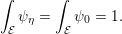 $$\begin{eqnarray}\int _{{\mathcal{E}}}{\it\psi}_{{\it\eta}}=\int _{{\mathcal{E}}}{\it\psi}_{0}=1.\end{eqnarray}$$
It can also be shown by a direct computation that  $f_{{\it\eta}}\geqslant 0$: see Remark 5.3 below.
Proof. Let us first show that  $(\widetilde{{\mathcal{L}}}{\mathcal{L}}_{0}^{-1})^{\ast }$ is a bounded operator on
 $L_{0}^{2}({\it\psi}_{0})$. To this end, we show that its adjoint
 $\widetilde{{\mathcal{L}}}{\mathcal{L}}_{0}^{-1}$ is bounded from
 $L_{0}^{2}({\it\psi}_{0})$ to
 $L^{2}({\it\psi}_{0})$. For
 $C^{\infty }$ and compactly supported functions
 ${\it\varphi}$,
 $$\begin{eqnarray}\frac{{\it\gamma}}{{\it\beta}}\Vert {\rm\nabla}_{p}{\it\varphi}\Vert _{L^{2}({\it\psi}_{0})}^{2}=-\langle {\mathcal{L}}_{0}{\it\varphi},{\it\varphi}\rangle _{L^{2}({\it\psi}_{0})}\leqslant \Vert {\mathcal{L}}_{0}{\it\varphi}\Vert _{L^{2}({\it\psi}_{0})}\Vert {\it\varphi}\Vert _{L^{2}({\it\psi}_{0})},\end{eqnarray}$$
so that
 $$\begin{eqnarray}\Vert \widetilde{{\mathcal{L}}}{\it\varphi}\Vert _{L^{2}({\it\psi}_{0})}^{2}\leqslant \Vert {\rm\nabla}_{p}{\it\varphi}\Vert _{L^{2}({\it\psi}_{0})}^{2}\leqslant \frac{{\it\beta}}{{\it\gamma}}\Vert {\mathcal{L}}_{0}{\it\varphi}\Vert _{L^{2}({\it\psi}_{0})}\Vert {\it\varphi}\Vert _{L^{2}({\it\psi}_{0})}.\end{eqnarray}$$
Since  ${\mathcal{L}}_{0}$ is invertible on
 $L_{0}^{2}({\it\psi}_{0})$ by Corollary 2.21, it follows that, for any
 ${\it\varphi}\in L_{0}^{2}({\it\psi}_{0})$,
 $$\begin{eqnarray}\Vert \widetilde{{\mathcal{L}}}{\mathcal{L}}_{0}^{-1}{\it\varphi}\Vert _{L^{2}({\it\psi}_{0})}^{2}\leqslant \frac{{\it\beta}}{{\it\gamma}}\Vert {\it\varphi}\Vert _{L^{2}({\it\psi}_{0})}\Vert {\mathcal{L}}_{0}^{-1}{\it\varphi}\Vert _{L^{2}({\it\psi}_{0})}.\end{eqnarray}$$
The operator  $\widetilde{{\mathcal{L}}}{\mathcal{L}}_{0}^{-1}$ is therefore bounded from
 $L_{0}^{2}({\it\psi}_{0})$ to
 $L^{2}({\it\psi}_{0})$, with operator norm bounded from above by
 ${\it\beta}\Vert {\mathcal{L}}_{0}^{-1}\Vert _{{\mathcal{B}}(L^{2}({\it\psi}_{0}))}/{\it\gamma}$. Denoting by
 ${\rm\Pi}_{0}$ the projection operator
 $$\begin{eqnarray}{\rm\Pi}_{0}{\it\varphi}={\it\varphi}-\int _{{\mathcal{E}}}{\it\varphi}\,{\it\psi}_{0},\end{eqnarray}$$
it follows that the operator  ${\rm\Pi}_{0}\widetilde{{\mathcal{L}}}{\mathcal{L}}_{0}^{-1}$ is bounded on
 $L_{0}^{2}({\it\psi}_{0})$, so that its adjoint
 $(\widetilde{{\mathcal{L}}}{\mathcal{L}}_{0}^{-1})^{\ast }{\rm\Pi}_{0}$ is also bounded on
 $L_{0}^{2}({\it\psi}_{0})$. In fact,
 $(\widetilde{{\mathcal{L}}}{\mathcal{L}}_{0}^{-1})^{\ast }{\rm\Pi}_{0}=(\widetilde{{\mathcal{L}}}{\mathcal{L}}_{0}^{-1})^{\ast }$ on
 $L_{0}^{2}({\it\psi}_{0})$, which proves that
 $(\widetilde{{\mathcal{L}}}{\mathcal{L}}_{0}^{-1})^{\ast }$ is bounded on
 $L_{0}^{2}({\it\psi}_{0})$ with operator norm bounded from above by
 ${\it\beta}\Vert {\mathcal{L}}_{0}^{-1}\Vert _{{\mathcal{B}}(L^{2}({\it\psi}_{0}))}/{\it\gamma}$. As a consequence the spectral radius
 $r$ satisfies
 $r\leqslant {\it\beta}\Vert {\mathcal{L}}_{0}^{-1}\Vert _{{\mathcal{B}}(L^{2}({\it\psi}_{0}))}/{\it\gamma}$.
It is then easy to check that (5.11) is a convergent series in  $L^{2}({\it\psi}_{0})$ when
 $|{\it\eta}|r<1$, since the series
 $$\begin{eqnarray}\mathop{\sum }_{n=1}^{+\infty }(-{\it\eta})^{n}[(\widetilde{{\mathcal{L}}}{\mathcal{L}}_{0}^{-1})^{\ast }]^{n}\end{eqnarray}$$
converges in  ${\mathcal{B}}(L_{0}^{2}({\it\psi}_{0}))$. Therefore, the function
 $f_{{\it\eta}}$ defined by (5.11) is well defined in
 $L^{2}({\it\psi}_{0})$. Henceforth we denote
 $\widetilde{{\it\psi}}_{{\it\eta}}=f_{{\it\eta}}{\it\psi}_{0}$. Note that
 $\int _{{\mathcal{E}}}\widetilde{{\it\psi}}_{{\it\eta}}=1$ since
 $f_{{\it\eta}}-\mathbf{1}\in L_{0}^{2}({\it\psi}_{0})$.
Our aim is to prove that  ${\it\psi}_{{\it\eta}}=\widetilde{{\it\psi}}_{{\it\eta}}$. To this end, we consider the following characterization
of the invariant probability measure: for any
 $C^{\infty }$ and compactly supported function
 ${\it\varphi}$,
 $$\begin{eqnarray}\int _{{\mathcal{E}}}(\text{e}^{t{\mathcal{L}}_{{\it\eta}}}{\it\varphi}){\it\psi}_{{\it\eta}}=\int _{{\mathcal{E}}}{\it\varphi}\,{\it\psi}_{{\it\eta}},\quad \text{for all }t\geqslant 0.\end{eqnarray}$$
The same equality holds with  ${\it\psi}_{{\it\eta}}$ replaced by
 $\widetilde{{\it\psi}}_{{\it\eta}}$. Indeed, a straightforward computation shows that, by
definition of
 $f_{{\it\eta}}$,
 $$\begin{eqnarray}{\mathcal{L}}_{{\it\eta}}^{\ast }f_{{\it\eta}}={\mathcal{L}}_{0}^{\ast }(1+{\it\eta}(\widetilde{{\mathcal{L}}}{\mathcal{L}}_{0}^{-1})^{\ast })f_{{\it\eta}}={\mathcal{L}}_{0}^{\ast }\mathbf{1}=0.\end{eqnarray}$$
Therefore,  $\text{e}^{t{\mathcal{L}}_{{\it\eta}}^{\ast }}f_{{\it\eta}}=f_{{\it\eta}}$ for all
 $t\geqslant 0$. The measure
 $\widetilde{{\it\psi}}_{{\it\eta}}=f_{{\it\eta}}{\it\psi}_{0}$ is therefore such that, for all
 ${\it\varphi}\in L^{2}({\it\psi}_{0})$ and all
 $t\geqslant 0$,
 $$\begin{eqnarray}\int _{{\mathcal{E}}}(\text{e}^{t{\mathcal{L}}_{{\it\eta}}}{\it\varphi})\widetilde{{\it\psi}}_{{\it\eta}}=\int _{{\mathcal{E}}}{\it\varphi}\,(\text{e}^{t{\mathcal{L}}_{{\it\eta}}^{\ast }}f_{{\it\eta}}){\it\psi}_{0}=\int _{{\mathcal{E}}}{\it\varphi}\,f_{{\it\eta}}{\it\psi}_{0}=\int _{{\mathcal{E}}}{\it\varphi}\,\widetilde{{\it\psi}}_{{\it\eta}}.\end{eqnarray}$$
This equality is true in particular for bounded, measurable functions.
However, it is not possible to conclude at this stage that  ${\it\psi}_{{\it\eta}}=\widetilde{{\it\psi}}_{{\it\eta}}$, because (5.14) characterizes invariant probability measures, whereas it is
not clear that
 $\widetilde{{\it\psi}}_{{\it\eta}}$ is a probability measure: the non-negativity of
the density is not guaranteed (but see Remark 5.3 below, which provides an
alternative way to conclude the proof presented here). To prove
non-negativity, we rely on the ergodicity of the continuous dynamics: for
any bounded measurable function
 ${\it\varphi}$ and any initial condition
 $(q_{0},p_{0})\in {\mathcal{E}}$, ergodicity of the Langevin dynamicsFootnote 16 implies
 $$\begin{eqnarray}\mathbb{E}^{(q_{0},p_{0})}\biggl(\frac{1}{t}\int _{0}^{t}{\it\varphi}(q_{s},p_{s})\biggr)=\frac{1}{t}\int _{0}^{t}(\text{e}^{s{\mathcal{L}}_{{\it\eta}}}{\it\varphi})(q_{0},p_{0})\,\text{d}s\xrightarrow[t\rightarrow +\infty ]{}\int _{{\mathcal{E}}}{\it\varphi}\,{\it\psi}_{{\it\eta}},\end{eqnarray}$$
so that, using Fubini’s theorem to justify the first equality and the dominated convergence theorem for the limit,
 $$\begin{eqnarray}\frac{1}{t}\int _{0}^{t}\biggl(\int _{{\mathcal{E}}}(\text{e}^{s{\mathcal{L}}_{{\it\eta}}}{\it\varphi})\,\widetilde{{\it\psi}}_{{\it\eta}}\biggr)\,\text{d}s=\int _{{\mathcal{E}}}\biggl(\frac{1}{t}\int _{0}^{t}\text{e}^{s{\mathcal{L}}_{{\it\eta}}}{\it\varphi}\,\text{d}s\biggr)\widetilde{{\it\psi}}_{{\it\eta}}\xrightarrow[t\rightarrow +\infty ]{}\int _{{\mathcal{E}}}{\it\varphi}\,{\it\psi}_{{\it\eta}}.\end{eqnarray}$$
Since, for any  $t>0$,
 $$\begin{eqnarray}\frac{1}{t}\int _{0}^{t}\biggl(\int _{{\mathcal{E}}}(\text{e}^{s{\mathcal{L}}_{{\it\eta}}}{\it\varphi})\,\widetilde{{\it\psi}}_{{\it\eta}}\biggr)\,\text{d}s=\int _{{\mathcal{E}}}{\it\varphi}\,\widetilde{{\it\psi}}_{{\it\eta}},\end{eqnarray}$$
we conclude that
 $$\begin{eqnarray}\int _{{\mathcal{E}}}{\it\varphi}\,\widetilde{{\it\psi}}_{{\it\eta}}=\int _{{\mathcal{E}}}{\it\varphi}\,{\it\psi}_{{\it\eta}}.\end{eqnarray}$$
This shows that  $\widetilde{{\it\psi}}_{{\it\eta}}={\it\psi}_{{\it\eta}}$. In particular,
 $\widetilde{{\it\psi}}_{{\it\eta}}\geqslant 0$.
Remark 5.3 (positivity of the invariant measure).
It is possible to prove directly the positivity of the invariant density  $f_{{\it\eta}}{\it\psi}_{0}$ by introducing the following Poisson equation:
 $$\begin{eqnarray}{\mathcal{L}}_{{\it\eta}}{\rm\Phi}_{{\it\eta}}=\mathbf{1}_{\{f_{{\it\eta}}\leqslant 0\}}-\int _{{\mathcal{E}}}\mathbf{1}_{\{f_{{\it\eta}}\leqslant 0\}}\,{\it\psi}_{{\it\eta}},\quad \int _{{\mathcal{E}}}{\rm\Phi}_{{\it\eta}}\,{\it\psi}_{{\it\eta}}=0,\end{eqnarray}$$
where  $f_{{\it\eta}}$ is defined by (5.11). This equation is well posed since
 ${\mathcal{L}}_{{\it\eta}}$ is invertible on weighted
 $L^{\infty }$-spaces of functions with average 0 with respect to
 ${\it\psi}_{{\it\eta}}$ (see the discussion after Proposition 5.1). Now, by the definition
(5.11) of
 $f_{{\it\eta}}$,
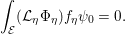 $$\begin{eqnarray}\int _{{\mathcal{E}}}({\mathcal{L}}_{{\it\eta}}{\rm\Phi}_{{\it\eta}})f_{{\it\eta}}{\it\psi}_{0}=0.\end{eqnarray}$$
On the other hand, by definition of  ${\rm\Phi}_{{\it\eta}}$,
 $$\begin{eqnarray}\displaystyle \int _{{\mathcal{E}}}({\mathcal{L}}_{{\it\eta}}{\rm\Phi}_{{\it\eta}})f_{{\it\eta}}{\it\psi}_{0} & = & \displaystyle \int _{{\mathcal{E}}}\mathbf{1}_{\{f_{{\it\eta}}\leqslant 0\}}f_{{\it\eta}}\,{\it\psi}_{0}-\biggl(\int _{{\mathcal{E}}}\mathbf{1}_{\{f_{{\it\eta}}\leqslant 0\}}\,{\it\psi}_{{\it\eta}}\biggr)\int _{{\mathcal{E}}}f_{{\it\eta}}{\it\psi}_{0}\nonumber\\ \displaystyle & = & \displaystyle \int _{{\mathcal{E}}}\mathbf{1}_{\{f_{{\it\eta}}\leqslant 0\}}f_{{\it\eta}}\,{\it\psi}_{0}-\int _{{\mathcal{E}}}\mathbf{1}_{\{f_{{\it\eta}}\leqslant 0\}}\,{\it\psi}_{{\it\eta}}.\nonumber\end{eqnarray}$$
The first integral on the right-hand side of the previous
equality is non-positive, while the second one is non-negative; hence the
quantity on the right-hand side is non-positive. Since the right-hand side
is equal to 0 by (5.16), each term must be 0. This allows us
to conclude that  $f_{{\it\eta}}\geqslant 0$ almost everywhere (using the first integral, since
 ${\it\psi}_{0}$ has a positive density with respect to the Lebesgue
measure).
5.2.3 Reformulating the linear response as an integrated correlation
A very useful corollary of (5.12)–(5.13) is the following reformulation of the linear response
definition (5.10)
of the transport coefficient through the celebrated Green–Kubo formula.
To state it, we introduce the conjugate response function, formally defined as  $S=\widetilde{{\mathcal{L}}}^{\ast }\mathbf{1}$. Its expression is found in practice by integration by parts, as
follows: for any
 $C^{\infty }$ compactly supported function
 ${\it\varphi}$,
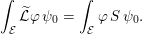 $$\begin{eqnarray}\int _{{\mathcal{E}}}\widetilde{{\mathcal{L}}}{\it\varphi}\,{\it\psi}_{0}=\int _{{\mathcal{E}}}{\it\varphi}\,S\,{\it\psi}_{0}.\end{eqnarray}$$
Note that the expression of  $S$ is determined by the applied perturbation
 $\widetilde{{\mathcal{L}}}$, and not by the response function
 $R$ chosen in (5.10). For the non-equilibrium Langevin dynamics (5.1), a simple computation shows
that
 $$\begin{eqnarray}S(q,p)={\it\beta}R(q,p)={\it\beta}F^{T}M^{-1}p.\end{eqnarray}$$
Note that  $S\in L_{0}^{2}({\it\psi}_{0})$ in this case.
Proposition 5.4 (Green–Kubo formula).
Consider the non-equilibrium Langevin dynamics (5.1) and the
definition (5.17) of the conjugate function  $S$. Then, for any
 $R\in L_{0}^{2}({\it\psi}_{0})$,
 $$\begin{eqnarray}\lim _{{\it\eta}\rightarrow 0}\frac{\mathbb{E}_{{\it\eta}}(R)}{{\it\eta}}=\int _{0}^{+\infty }\mathbb{E}_{0}(R(q_{t},p_{t})S(q_{0},p_{0}))\,\text{d}t,\end{eqnarray}$$
where  $\mathbb{E}_{{\it\eta}}$ is an average with respect to the invariant measure
 ${\it\psi}_{{\it\eta}}(q,p)\,\text{d}q\,\text{d}p$ of the non-equilibrium dynamics (5.1), while the expectation
 $\mathbb{E}_{0}$ on the right-hand side is taken over all initial
conditions distributed according to the canonical measure
 ${\it\psi}_{0}(q,p)\,\text{d}q\,\text{d}p$, and over all realizations of the reference equilibrium
dynamics with generator
 ${\mathcal{L}}_{0}$.
The Green–Kubo formula thus shows that a non-equilibrium property
(namely the transport coefficient  ${\it\rho}_{F}=\lim _{{\it\eta}\rightarrow 0}\mathbb{E}_{{\it\eta}}(R)/{\it\eta}$ of the left-hand side of (5.18)) can be obtained using simulations at equilibrium,
namely for
 ${\it\eta}=0$ (see the right-hand side of (5.18)). This result can easily be generalized to other
dynamics when the perturbation
 $\widetilde{{\mathcal{L}}}$ is such that
 $S\in L^{2}({\it\psi}_{0})$ and the linear response result (5.12) holds (see
Section 5.2.4 for possible
assumptions on
 $\widetilde{{\mathcal{L}}}$).
Proof. In view of (5.10), (5.12) and (5.13), as well as the equality
 $$\begin{eqnarray}-{\mathcal{L}}_{0}^{-1}=\int _{0}^{+\infty }\text{e}^{t{\mathcal{L}}_{0}}\,\text{d}t\end{eqnarray}$$
as operators on  $L_{0}^{2}({\it\psi}_{0})$ (as given by Corollary 2.21), we can write, for
 $R\in L_{0}^{2}({\it\psi}_{0})$,
 $$\begin{eqnarray}\displaystyle \lim _{{\it\eta}\rightarrow 0}\frac{\mathbb{E}_{{\it\eta}}(R)}{{\it\eta}} & = & \displaystyle \int _{{\mathcal{E}}}R\,\mathfrak{f}_{1}\,{\it\psi}_{0}=-\int _{{\mathcal{E}}}[{\mathcal{L}}_{0}^{-1}R][\widetilde{{\mathcal{L}}}^{\ast }\mathbf{1}]\,{\it\psi}_{0}\nonumber\\ \displaystyle & = & \displaystyle \int _{0}^{+\infty }\mathbb{E}(R(q_{t},p_{t})S(q_{0},p_{0}))\,\text{d}t,\nonumber\end{eqnarray}$$
which gives the claimed result.
Let us rewrite equation (5.18) more precisely in the context of (5.1). The mobility  ${\it\rho}_{F}$ in the direction
 $F$, defined in (5.10), is equal to
 ${\it\beta}$ times the integrated velocity autocorrelation:
 $$\begin{eqnarray}{\it\rho}_{F}=\lim _{{\it\eta}\rightarrow 0}\frac{\mathbb{E}_{{\it\eta}}(F\cdot M^{-1}p)}{{\it\eta}}={\it\beta}\int _{0}^{+\infty }\mathbb{E}_{0}((F\cdot M^{-1}p_{t})(F\cdot M^{-1}p_{0}))\,\text{d}t.\end{eqnarray}$$
5.2.4 Generalization to other dynamics
It is of course possible to generalize linear response results and Green–Kubo formulae to dynamics other than (5.1), either by generalizing the assumptions ensuring that Theorem 5.2 and Proposition 5.4 hold (as we do below), or by working with a different set of assumptions as in Assaraf, Jourdain, Lelièvre and Roux (Reference Assaraf, Jourdain, Lelièvre and Roux2015).
An inspection of the proof of Theorem 5.2 shows that the result can be generalized to other
perturbations, and in fact to other reference equilibrium dynamics  $(x_{t}^{{\it\eta}})_{t\geqslant 0}$ with generator
 ${\mathcal{L}}_{{\it\eta}}={\mathcal{L}}_{0}+{\it\eta}\widetilde{{\mathcal{L}}}$, under the following conditions.
(a) Existence of a unique invariant measure. For any
${\it\eta}\in \mathbb{R}$, the perturbed dynamics admits a unique invariant
measure with $C^{\infty }$ density ${\it\psi}_{{\it\eta}}(x)$ with respect to the Lebesgue measure $\text{d}x$ on ${\mathcal{X}}$. Such results can be proved with the techniques from
Section 2.4.(b) Ergodicity of the perturbed dynamics. The perturbed dynamics is ergodic in the following sense: for any bounded measurable function
${\it\varphi}$ and almost all initial condition $x_{0}$, See Section 3.1 for techniques to obtain such convergence results.$$\begin{eqnarray}\frac{1}{t}\int _{0}^{t}{\it\varphi}(x_{s})\,\text{d}s\xrightarrow[t\rightarrow +\infty ]{}\int _{{\mathcal{X}}}{\it\varphi}\,{\it\psi}_{{\it\eta}}\quad \text{almost surely.}\end{eqnarray}$$Alternatively, as discussed in Remark 5.3, the ergodicity condition can be replaced with solvability conditions for the Poisson equation (5.15).
(c) Properties of the equilibrium dynamics.
$\text{Ker}({\mathcal{L}}_{0}^{\ast })=\mathbf{1}$ and ${\mathcal{L}}_{0}^{\ast }$ is invertible on $L_{0}^{2}({\it\psi}_{0})$. See Corollary 2.4 for overdamped Langevin dynamics and
Corollary 2.21 for Langevin dynamics.(d) Properties of the perturbation.
$\text{Ran}(\widetilde{{\mathcal{L}}}^{\ast })\subset L_{0}^{2}({\it\psi}_{0})$ and $(\widetilde{{\mathcal{L}}}{\mathcal{L}}_{0}^{-1})^{\ast }$ is bounded on $L_{0}^{2}({\it\psi}_{0})$. Note that, if $\widetilde{{\mathcal{L}}}\mathbf{1}=0$, then the function $\widetilde{{\mathcal{L}}}^{\ast }{\it\varphi}$ has average 0 with respect to ${\it\psi}_{0}$: $$\begin{eqnarray}\int _{{\mathcal{X}}}\widetilde{{\mathcal{L}}}^{\ast }{\it\varphi}\,{\it\psi}_{0}=\int _{{\mathcal{X}}}{\it\varphi}\,\widetilde{{\mathcal{L}}}\mathbf{1}\,{\it\psi}_{0}=0.\end{eqnarray}$$





The last condition, namely that  $(\widetilde{{\mathcal{L}}}{\mathcal{L}}_{0}^{-1})^{\ast }$ is bounded on
 $L_{0}^{2}({\it\psi}_{0})$, expresses the fact that the perturbation
 $\widetilde{{\mathcal{L}}}$ is sufficiently small. A typical way of proving that
 $(\widetilde{{\mathcal{L}}}{\mathcal{L}}_{0}^{-1})^{\ast }$ is bounded on
 $L_{0}^{2}({\it\psi}_{0})$ is, as at the beginning of the proof of Theorem 5.2, to show that
 $\widetilde{{\mathcal{L}}}$ is
 ${\mathcal{L}}_{0}$-bounded, namely that there exist
 $a,b>0$ such that, for all
 $C^{\infty }$ and compactly supported functions
 ${\it\varphi}$,
 $$\begin{eqnarray}\Vert \widetilde{{\mathcal{L}}}{\it\varphi}\Vert _{L^{2}({\it\psi}_{0})}\leqslant a\Vert {\mathcal{L}}_{0}{\it\varphi}\Vert _{L^{2}({\it\psi}_{0})}+b\Vert {\it\varphi}\Vert _{L^{2}({\it\psi}_{0})}.\end{eqnarray}$$
Then, for all  ${\it\varphi}\in L_{0}^{2}({\it\psi}_{0})$,
 $$\begin{eqnarray}\Vert \widetilde{{\mathcal{L}}}{\mathcal{L}}_{0}^{-1}{\it\varphi}\Vert _{L^{2}({\it\psi}_{0})}\leqslant a\Vert {\it\varphi}\Vert _{L^{2}({\it\psi}_{0})}+b\Vert {\mathcal{L}}_{0}^{-1}{\it\varphi}\Vert _{L^{2}({\it\psi}_{0})},\end{eqnarray}$$
so that  $\widetilde{{\mathcal{L}}}{\mathcal{L}}_{0}^{-1}$, and its adjoint, are bounded operators on
 $L_{0}^{2}({\it\psi}_{0})$ with operator norm bounded by
 $a+b\Vert {\mathcal{L}}_{0}^{-1}\Vert _{{\mathcal{B}}(L_{0}^{2}({\it\psi}_{0}))}$.
Remark 5.5 (stronger perturbations).
There are situations for which the condition (5.20) is not satisfied. This
is the case for generalizations of the dynamics (5.2), for which the
perturbation operator  $\widetilde{{\mathcal{L}}}$ involves second derivatives of the momenta
 $p$, whereas
 ${\mathcal{L}}_{0}$ may control only first-order derivatives. In this case, it
is not possible to write an expansion of the invariant measure as a power
series in
 ${\it\eta}$. Nonetheless, linear response results on average
properties can still be stated by following the same strategy as in the
proof of Theorem 3.3. To this end, we assume that Assumption 3.2 is satisfied for
 ${\mathcal{A}}_{1}={\mathcal{L}}_{0}$ and
 ${\mathcal{A}}_{1}={\mathcal{L}}_{0}^{\ast }$. First, introduce
 $\mathfrak{f}_{1}$ such that
 $$\begin{eqnarray}\int _{{\mathcal{X}}}[({\mathcal{L}}_{0}+{\it\eta}\widetilde{{\mathcal{L}}}){\it\varphi}](1+{\it\eta}\mathfrak{f}_{1}){\it\psi}_{0}=\text{O}({\it\eta}^{2}).\end{eqnarray}$$
A simple computation shows that  $\mathfrak{f}_{1}$ is formally given by (5.12). In fact,
 $\mathfrak{f}_{1}=-({\mathcal{L}}_{0}^{\ast })^{-1}S$, where
 $S$ is defined in (5.17). We next replace
 ${\it\varphi}$ by
 $Q_{{\it\eta}}{\it\varphi}$, where
 $Q_{{\it\eta}}$ is the approximate inverse
 $$\begin{eqnarray}Q_{{\it\eta}}={\rm\Pi}_{0}{\mathcal{L}}_{0}^{-1}{\rm\Pi}_{0}-{\it\eta}{\rm\Pi}_{0}{\mathcal{L}}_{0}^{-1}{\rm\Pi}_{0}\widetilde{{\mathcal{L}}}{\rm\Pi}_{0}{\mathcal{L}}_{0}^{-1}{\rm\Pi}_{0}.\end{eqnarray}$$
The operator  $Q_{{\it\eta}}$ is a well-defined operator acting on
 $C^{\infty }$ functions with zero average with respect to
 ${\it\psi}_{0}$. It can therefore be shown that, under moment conditions
on the invariant measure (that is,
 ${\it\psi}_{{\it\eta}}$ integrates all the scale functions appearing in
Definition 3.1),
 $$\begin{eqnarray}\int _{{\mathcal{X}}}{\it\varphi}\,{\it\psi}_{{\it\eta}}=\int _{{\mathcal{X}}}{\it\varphi}\,{\it\psi}_{0}+{\it\eta}\int _{{\mathcal{X}}}{\it\varphi}\,\mathfrak{f}_{1}\,{\it\psi}_{0}+{\it\eta}^{2}r_{{\it\varphi},{\it\eta}},\end{eqnarray}$$
where  $|r_{{\it\varphi},{\it\eta}}|\leqslant K$ for
 $|{\it\eta}|$ sufficiently small.
5.3 Error estimates on the computation of transport coefficients
The results of the previous section show that there are two ways to compute transport coefficients, either by discretizing the integrated correlation function based on the Green–Kubo formula (5.18), or by approximating the derivative of equilibrium averages with respect to the magnitude of the external forcing as in (5.10). In this section we provide, for both approaches, error estimates on the bias generated by the use of finite time steps to integrate the dynamics. The results quoted here were first presented in Leimkuhler et al. (Reference Leimkuhler, Matthews and Stoltz2015).
5.3.1 Green–Kubo formulae
We first provide error estimates on linear responses computed using
Green–Kubo formulae such as (5.18). We state the result on a general space  ${\mathcal{X}}$ for a general dynamics (3.1) with generator
 ${\mathcal{L}}$ (instead of the notation
 ${\mathcal{L}}_{0}$ used in Section 5.2). The precise result is formulated for smooth functions in the sense
of Definition 3.1. We
let
 ${\it\pi}$ denote the reference invariant measure, and still suppose that
Assumption 3.2 holds
with
 ${\mathcal{A}}_{1}={\mathcal{L}}$ (i.e., the space
 ${\mathcal{S}}$ introduced in Definition 3.1 is dense in
 $L^{2}({\it\pi})$ and the operator
 ${\mathcal{L}}^{-1}:{\mathcal{S}}_{0}\rightarrow {\mathcal{S}}_{0}$ is well defined, where
 ${\mathcal{S}}_{0}$ is defined in (3.16)).
As in Section 3.2, we consider a
discretization of the continuous dynamics under consideration, with transition
operator  $P_{{\rm\Delta}t}$, and let
 ${\it\pi}_{{\rm\Delta}t}$ denote an invariant measure of the numerical scheme (see
Section 3.2.2 for a
discussion of possible conditions ensuring the existence of an invariant measure).
We also introduce the projection operator
 $$\begin{eqnarray}{\rm\Pi}_{{\rm\Delta}t}{\it\varphi}={\it\varphi}-\int _{{\mathcal{X}}}{\it\varphi}\,\text{d}{\it\pi}_{{\rm\Delta}t},\end{eqnarray}$$
as well as
 $$\begin{eqnarray}L_{{\mathcal{K}}_{s},{\rm\Delta}t}^{\infty }({\mathcal{X}})={\rm\Pi}_{{\rm\Delta}t}L_{{\mathcal{K}}_{s}}^{\infty }({\mathcal{X}})=\biggl\{{\it\varphi}\in L_{{\mathcal{K}}_{s}}^{\infty }({\mathcal{X}})\,\bigg|\,\int _{{\mathcal{X}}}{\it\varphi}\,\text{d}{\it\pi}_{{\rm\Delta}t}=0\biggr\}.\end{eqnarray}$$
The range of  ${\rm\Pi}_{{\rm\Delta}t}$ is contained in the set of functions with average zero with
respect to the invariant measure
 ${\it\pi}_{{\rm\Delta}t}$ of the numerical scheme.
Theorem 5.6 (error estimates for Green–Kubo).
Consider a numerical method with an invariant measure  ${\it\pi}_{{\rm\Delta}t}$ which integrates any scale function
 ${\mathcal{K}}_{n}$ introduced in Definition 3.1. Assume that there exists an
integer
 ${\it\alpha}\geqslant 1$, such that, for any observable
 ${\it\phi}\in {\mathcal{S}}$, there is
 $K,{\rm\Delta}t^{\ast }>0$ for which the following conditions hold.
(i) Error on the invariant measure:
(5.21)with$$\begin{eqnarray}\int _{{\mathcal{X}}}{\it\phi}\,\text{d}{\it\pi}_{{\rm\Delta}t}=\int _{{\mathcal{X}}}{\it\phi}\,\text{d}{\it\pi}+{\rm\Delta}t^{{\it\alpha}}r_{{\it\phi},{\rm\Delta}t},\end{eqnarray}$$$|r_{{\it\phi},{\rm\Delta}t}|\leqslant K$ for $0<{\rm\Delta}t\leqslant {\rm\Delta}t^{\ast }$.(ii) Expansion of
$P_{{\rm\Delta}t}$: (5.22)where the operators$$\begin{eqnarray}-\frac{\text{Id}-P_{{\rm\Delta}t}}{{\rm\Delta}t}{\it\phi}={\mathcal{L}}{\it\phi}+{\rm\Delta}tS_{1}{\it\phi}+\cdots +{\rm\Delta}t^{{\it\alpha}-1}S_{{\it\alpha}-1}{\it\phi}+{\rm\Delta}t^{{\it\alpha}}\widetilde{R}_{{\it\alpha},{\rm\Delta}t}{\it\phi},\end{eqnarray}$$$S_{1},\ldots ,S_{{\it\alpha}-1},\widetilde{R}_{{\it\alpha},{\rm\Delta}t}$ (which are defined independently of ${\it\phi}$) are well defined on ${\mathcal{S}}$ with values in ${\mathcal{S}}$; and there exists $s_{0}\in \mathbb{N}$ (depending on ${\it\alpha}$ and ${\it\phi}$) such that $\Vert \widetilde{R}_{{\it\alpha},{\rm\Delta}t}{\it\phi}\Vert _{L_{{\mathcal{K}}_{s_{0}}}^{\infty }}\leqslant K$ for $0<{\rm\Delta}t\leqslant {\rm\Delta}t^{\ast }$.







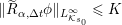

Moreover, we assume the following.
(iii) Uniform-in-
${\rm\Delta}t$ exponential convergence of $P_{{\rm\Delta}t}$. For any $s\geqslant 0$, there exist $C_{s},{\it\lambda}_{s}>0$ such that, for all $0<{\rm\Delta}t\leqslant {\rm\Delta}t^{\ast }$, (5.23)$$\begin{eqnarray}\Vert P_{{\rm\Delta}t}^{n}\Vert _{{\mathcal{B}}(L_{{\mathcal{K}}_{s},{\rm\Delta}t}^{\infty })}\leqslant C_{s}\,\text{e}^{-{\it\lambda}_{s}n{\rm\Delta}t},\quad \text{for all }n\in \mathbb{N}.\end{eqnarray}$$



Then, the integrated correlation of two observables  ${\it\psi},{\it\varphi}\in {\mathcal{S}}_{0}$ can be approximated by a Riemann sum up to an error of
order
 ${\rm\Delta}t^{{\it\alpha}}$: there exists
 $R>0$ such that
 $$\begin{eqnarray}\int _{0}^{+\infty }\mathbb{E}_{{\it\pi}}({\it\psi}(x_{t}){\it\varphi}(x_{0}))\,\text{d}t={\rm\Delta}t\mathop{\sum }_{n=0}^{+\infty }\mathbb{E}_{{\it\pi}_{{\rm\Delta}t}}(\widetilde{{\it\psi}}_{{\rm\Delta}t,{\it\alpha}}(x^{n}){\it\varphi}(x^{0}))+{\rm\Delta}t^{{\it\alpha}}r_{{\rm\Delta}t}^{{\it\psi},{\it\varphi}},\end{eqnarray}$$
with  $|r_{{\rm\Delta}t}^{{\it\psi},{\it\varphi}}|\leqslant R$ for
 $0<{\rm\Delta}t\leqslant {\rm\Delta}t^{\ast }$. In this expression, the expectation
 $\mathbb{E}_{{\it\pi}}$ is over all initial conditions
 $(q_{0},p_{0})\sim {\it\pi}$ and over all realizations of the continuous dynamics with
generator
 ${\mathcal{L}}$, while the expectation
 $\mathbb{E}_{{\it\pi}_{{\rm\Delta}t}}$ is over all initial conditions
 $(q_{0},p_{0})\sim {\it\pi}_{{\rm\Delta}t}$ and over all realizations of the Markov chain induced by
 $P_{{\rm\Delta}t}$. Moreover, the modified observable
 $\widetilde{{\it\psi}}_{{\rm\Delta}t,{\it\alpha}}\in {\mathcal{S}}$ is defined as
 $\widetilde{{\it\psi}}_{{\rm\Delta}t,{\it\alpha}}={\rm\Pi}_{{\rm\Delta}t}{\it\psi}_{{\rm\Delta}t,{\it\alpha}}$ with
 $$\begin{eqnarray}{\it\psi}_{{\rm\Delta}t,{\it\alpha}}=(\text{Id}+{\rm\Delta}t\,S_{1}{\mathcal{L}}^{-1}+\cdots +{\rm\Delta}t^{{\it\alpha}-1}S_{{\it\alpha}-1}{\mathcal{L}}^{-1}){\it\psi}.\end{eqnarray}$$
This result deserves several comments, both on the three main assumptions (5.21), (5.22) and (5.23), as well as on the error estimate (5.24) itself. The proof is presented after this discussion.
Let us start with the assumptions of Theorem 5.6. Equation (5.21) can be proved by following the general strategy
presented in Theorem 3.3. Note that the remainder term in (5.21) can vanish, for example when
a Metropolis procedure is superimposed on the numerical scheme. In this case,  ${\it\alpha}$ is determined by (5.22). Condition (5.22) has already been encountered when proving error estimates on the
invariant measure (see (3.15)).
Finally, the uniform-in-
 ${\rm\Delta}t$ convergence (5.23) is given, for the Euler–Maruyama
discretization of overdamped Langevin dynamics, by (3.29), which is a consequence of the uniform minorization
condition of Lemma 3.4;
similar results exist for certain discretization of Langevin dynamics (see
Leimkuhler et al. Reference Leimkuhler, Matthews and Stoltz2015).
Let us now comment on the error estimate (5.24). First, the result shows that the error is of order  ${\rm\Delta}t^{{\it\alpha}}$, upon modifying the observable
 ${\it\psi}$ as
 $\widetilde{{\it\psi}}_{{\rm\Delta}t,{\it\alpha}}$. Therefore, a first limitation to the reduction of the error in
Green–Kubo formulae arises from the error on the invariant measure
itself. However, in practice, especially when
 ${\it\alpha}$ is large, the error is actually determined by the approximation
of the corrected observable
 $\widetilde{{\it\psi}}_{{\rm\Delta}t,{\it\alpha}}$. When the operators
 $S_{k}$ are powers of
 ${\mathcal{L}}$, the correction terms
 $S_{k}{\mathcal{L}}^{-1}{\it\psi}$ in (5.25) can
be easily computed. Let
 $k_{0}$ denote the last index for which
 $S_{k}{\mathcal{L}}^{-1}{\it\psi}$ can be evaluated. For example (see the discussion
after (3.15)), if
the discretization method is of weak order
 $k_{0}$, then
 $S_{k}={\mathcal{L}}^{k}/k!$ for all
 $k=1,\ldots ,k_{0}$, so that
 $S_{k}{\mathcal{L}}^{-1}{\it\psi}$ is easy to evaluate up to
 $k=k_{0}$. If
 $k_{0}<{\it\alpha}$, the error estimate which can be used in practice is
 $$\begin{eqnarray}\int _{0}^{+\infty }\mathbb{E}_{{\it\pi}}({\it\psi}(x_{t}){\it\varphi}(x_{0}))\,\text{d}t={\rm\Delta}t\mathop{\sum }_{n=0}^{+\infty }\mathbb{E}_{{\it\pi}_{{\rm\Delta}t}}(\widetilde{{\it\psi}}_{{\rm\Delta}t,k_{0}}(x^{n}){\it\varphi}(x^{0}))+{\rm\Delta}t^{k_{0}+1}r_{{\rm\Delta}t}^{{\it\psi},{\it\varphi}}.\end{eqnarray}$$
However, even if  ${\it\psi}_{{\rm\Delta}t,k_{0}}$ can be evaluated, it still remains to approximate
 $\widetilde{{\it\psi}}_{{\rm\Delta}t,k_{0}}={\rm\Pi}_{{\rm\Delta}t}{\it\psi}_{{\rm\Delta}t,k_{0}}$, typically by approximating the average of
 ${\it\psi}_{{\rm\Delta}t,k_{0}}$ with respect to
 ${\it\pi}_{{\rm\Delta}t}$ by trajectory averages.
Remark 5.7 (error estimates for Metropolis–Hastings dynamics).
For discretizations of the continuous dynamics stabilized by a
Metropolis–Hastings procedure, such as MALA for overdamped
Langevin, the invariant measure of the numerical scheme is exact by
construction. However, since the quantity  $S_{1}{\mathcal{L}}^{-1}{\it\psi}$ cannot be evaluated in general, the resulting
approximation of the integrated correlation is based on
 $\widetilde{{\it\psi}}_{{\rm\Delta}t,0}={\rm\Pi}_{{\rm\Delta}t}{\it\psi}$, which leads to an approximation of order
 ${\rm\Delta}t$ of the Green–Kubo integral. An error estimate
of order
 ${\rm\Delta}t^{3/2}$ can nevertheless be obtained by modifying the
Metropolis–Hastings proposal. It is even possible to obtain
errors of order
 ${\rm\Delta}t^{2}$ by modifying the Metropolis acceptance rule. See Fathi
et al. (Reference Fathi, Homman and Stoltz2014) and Fathi and Stoltz (Reference Fathi and Stoltz2015) for further details.
Let us now present the proof of Theorem 5.6.
Proof. Fix two observables  ${\it\varphi},{\it\psi}\in {\mathcal{S}}_{0}$. Note that
 $$\begin{eqnarray}\int _{0}^{+\infty }\mathbb{E}_{{\it\pi}}({\it\psi}(x_{t}){\it\varphi}(x_{0}))\,\text{d}t=\int _{{\mathcal{X}}}(-{\mathcal{L}}^{-1}{\it\psi}){\it\varphi}\,\text{d}{\it\pi}.\end{eqnarray}$$
In order to introduce the correlation functions of the
numerical scheme, we would like, in view of (5.22), to replace the measure  ${\it\pi}$ by
 ${\it\pi}_{{\rm\Delta}t}$ and the operator
 $-{\mathcal{L}}^{-1}$ by
 $$\begin{eqnarray}\biggl(\frac{\text{Id}-P_{{\rm\Delta}t}}{{\rm\Delta}t}\biggr)^{-1}={\rm\Delta}t\mathop{\sum }_{n=0}^{+\infty }P_{{\rm\Delta}t}^{n},\end{eqnarray}$$
However, this is not possible as such, for two reasons.
First, as indicated in (5.23), the above sum is only convergent when the
operators under consideration are restricted to subspaces of functions with
average 0 with respect to  ${\it\pi}_{{\rm\Delta}t}$. We therefore need to introduce the projections operators
 ${\rm\Pi}_{{\rm\Delta}t}$ to restrict
 ${\mathcal{L}}^{-1}$ to the range of
 ${\rm\Pi}_{{\rm\Delta}t}$. Second, it is not possible to consider the inverse of the
right-hand side of (5.22)
directly, so we will introduce
 $(\text{Id}-P_{{\rm\Delta}t})^{-1}(\text{Id}-P_{{\rm\Delta}t})$ instead, in order to retrieve some operator
 ${\mathcal{L}}$ to dominant order in
 ${\rm\Delta}t$, so as to cancel the inverse operator
 ${\mathcal{L}}^{-1}$.
Let us first introduce the projection operators  ${\rm\Pi}_{{\rm\Delta}t}$ and the invariant measure
 ${\it\pi}_{{\rm\Delta}t}$ of the numerical scheme, using the fact that
 $-{\mathcal{L}}^{-1}{\it\psi}$ has zero average with respect to
 ${\it\pi}$:
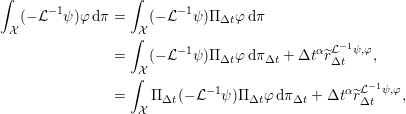 $$\begin{eqnarray}\displaystyle \int _{{\mathcal{X}}}(-{\mathcal{L}}^{-1}{\it\psi}){\it\varphi}\,\text{d}{\it\pi} & = & \displaystyle \int _{{\mathcal{X}}}(-{\mathcal{L}}^{-1}{\it\psi}){\rm\Pi}_{{\rm\Delta}t}{\it\varphi}\,\text{d}{\it\pi}\nonumber\\ \displaystyle & = & \displaystyle \int _{{\mathcal{X}}}(-{\mathcal{L}}^{-1}{\it\psi}){\rm\Pi}_{{\rm\Delta}t}{\it\varphi}\,\text{d}{\it\pi}_{{\rm\Delta}t}+{\rm\Delta}t^{{\it\alpha}}\widetilde{r}_{{\rm\Delta}t}^{{\mathcal{L}}^{-1}{\it\psi},{\it\varphi}},\nonumber\\ \displaystyle & = & \displaystyle \int _{{\mathcal{X}}}{\rm\Pi}_{{\rm\Delta}t}(-{\mathcal{L}}^{-1}{\it\psi}){\rm\Pi}_{{\rm\Delta}t}{\it\varphi}\,\text{d}{\it\pi}_{{\rm\Delta}t}+{\rm\Delta}t^{{\it\alpha}}\widetilde{r}_{{\rm\Delta}t}^{{\mathcal{L}}^{-1}{\it\psi},{\it\varphi}},\end{eqnarray}$$
where 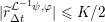 $|\widetilde{r}_{{\rm\Delta}t}^{{\mathcal{L}}^{-1}{\it\psi},{\it\varphi}}|\leqslant K/2$ for
 $0<{\rm\Delta}t\leqslant {\rm\Delta}t^{\ast }$ by (5.21) (possibly upon increasing the value of
 $K$ and decreasing
 ${\rm\Delta}t^{\ast }$).
The next step is to approximate  ${\rm\Pi}_{{\rm\Delta}t}(-{\mathcal{L}}^{-1}{\it\psi})$ in terms of powers of
 $P_{{\rm\Delta}t}$. We use the fact that
 ${\rm\Pi}_{{\rm\Delta}t}P_{{\rm\Delta}t}=P_{{\rm\Delta}t}{\rm\Pi}_{{\rm\Delta}t}$, and that
 $$\begin{eqnarray}\displaystyle {\rm\Pi}_{{\rm\Delta}t} & = & \displaystyle {\rm\Pi}_{{\rm\Delta}t}\biggl(\displaystyle \frac{\text{Id}-P_{{\rm\Delta}t}}{{\rm\Delta}t}\biggr)^{-1}\biggl(\displaystyle \frac{\text{Id}-P_{{\rm\Delta}t}}{{\rm\Delta}t}\biggr)\nonumber\\ \displaystyle & = & \displaystyle {\rm\Pi}_{{\rm\Delta}t}\biggl({\rm\Delta}t\mathop{\sum }_{n=0}^{+\infty }P_{{\rm\Delta}t}^{n}\biggr)\biggl(\displaystyle \frac{\text{Id}-P_{{\rm\Delta}t}}{{\rm\Delta}t}\biggr).\nonumber\end{eqnarray}$$
Note that the above sum is convergent in  ${\mathcal{B}}(L_{{\mathcal{K}}_{s},{\rm\Delta}t}^{\infty })$ in view of (5.23). Relying on (5.22),
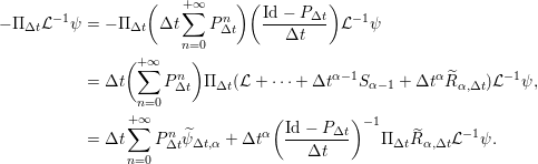 $$\begin{eqnarray}\displaystyle -{\rm\Pi}_{{\rm\Delta}t}{\mathcal{L}}^{-1}{\it\psi} & = & \displaystyle -{\rm\Pi}_{{\rm\Delta}t}\biggl({\rm\Delta}t\mathop{\sum }_{n=0}^{+\infty }P_{{\rm\Delta}t}^{n}\biggr)\biggl(\displaystyle \frac{\text{Id}-P_{{\rm\Delta}t}}{{\rm\Delta}t}\biggr){\mathcal{L}}^{-1}{\it\psi}\nonumber\\ \displaystyle & = & \displaystyle {\rm\Delta}t\biggl(\mathop{\sum }_{n=0}^{+\infty }P_{{\rm\Delta}t}^{n}\biggr){\rm\Pi}_{{\rm\Delta}t}({\mathcal{L}}+\cdots +{\rm\Delta}t^{{\it\alpha}-1}S_{{\it\alpha}-1}+{\rm\Delta}t^{{\it\alpha}}\widetilde{R}_{{\it\alpha},{\rm\Delta}t}){\mathcal{L}}^{-1}{\it\psi},\nonumber\\ \displaystyle & = & \displaystyle {\rm\Delta}t\mathop{\sum }_{n=0}^{+\infty }P_{{\rm\Delta}t}^{n}\widetilde{{\it\psi}}_{{\rm\Delta}t,{\it\alpha}}+{\rm\Delta}t^{{\it\alpha}}\biggl(\displaystyle \frac{\text{Id}-P_{{\rm\Delta}t}}{{\rm\Delta}t}\biggr)^{-1}{\rm\Pi}_{{\rm\Delta}t}\widetilde{R}_{{\it\alpha},{\rm\Delta}t}{\mathcal{L}}^{-1}{\it\psi}.\nonumber\end{eqnarray}$$
Note that the sums on the right-hand side are well defined in view of the decay estimates (5.23). Substituting the above equality in (5.26) leads to
 $$\begin{eqnarray}\displaystyle & & \displaystyle \int _{{\mathcal{X}}}(-{\mathcal{L}}^{-1}{\it\psi}){\it\varphi}\,\text{d}{\it\pi}={\rm\Delta}t\mathop{\sum }_{n=0}^{+\infty }\int _{{\mathcal{X}}}P_{{\rm\Delta}t}^{n}\widetilde{{\it\psi}}_{{\rm\Delta}t,{\it\alpha}}({\rm\Pi}_{{\rm\Delta}t}{\it\varphi})\,\text{d}{\it\pi}_{{\rm\Delta}t}\nonumber\\ \displaystyle & & \displaystyle \qquad +{\rm\Delta}t^{{\it\alpha}}\int _{{\mathcal{X}}}\biggl(\biggl(\displaystyle \frac{\text{Id}-P_{{\rm\Delta}t}}{{\rm\Delta}t}\biggr)^{-1}{\rm\Pi}_{{\rm\Delta}t}\widetilde{R}_{{\it\alpha},{\rm\Delta}t}{\mathcal{L}}^{-1}{\it\psi}\biggr){\rm\Pi}_{{\rm\Delta}t}{\it\varphi}\,\text{d}{\it\pi}_{{\rm\Delta}t}+{\rm\Delta}t^{{\it\alpha}}\widetilde{r}_{{\rm\Delta}t}^{{\mathcal{L}}^{-1}{\it\psi},{\it\varphi}}.\nonumber\end{eqnarray}$$
To conclude the proof, we use the fact that, for a given smooth function  $f$ and upon increasing
 $K$ and decreasing
 ${\rm\Delta}t^{\ast }$, there exist an integer
 $s$ and a constant
 $\widetilde{K}>0$ (depending on
 $f$) such that
 $\Vert \widetilde{R}_{{\it\alpha},{\rm\Delta}t}f\Vert _{L_{{\mathcal{K}}_{s}}^{\infty }}\leqslant \widetilde{K}$ for any
 ${\rm\Delta}t\in (0,{\rm\Delta}t^{\ast }]$. In addition, the following resolvent bound is directly
obtained from (5.23):
 $$\begin{eqnarray}\biggl\|\biggl(\displaystyle \frac{\text{Id}-P_{{\rm\Delta}t}}{{\rm\Delta}t}\biggr)^{-1}\biggr\|_{{\mathcal{B}}(L_{{\mathcal{K}}_{s},{\rm\Delta}t}^{\infty })}\leqslant \frac{C_{s}}{{\it\lambda}_{s}}.\end{eqnarray}$$
Finally,  ${\it\pi}_{{\rm\Delta}t}$ integrates all scale functions
 ${\mathcal{K}}_{n}$ by assumption. Therefore, upon increasing the value of
 $K$, the following inequality holds for any
 ${\rm\Delta}t\in (0,{\rm\Delta}t^{\ast }]$:
 $$\begin{eqnarray}\biggl|\int _{{\mathcal{X}}}\biggl(\biggl(\displaystyle \frac{\text{Id}-P_{{\rm\Delta}t}}{{\rm\Delta}t}\biggr)^{-1}{\rm\Pi}_{{\rm\Delta}t}\widetilde{R}_{{\it\alpha},{\rm\Delta}t}{\mathcal{L}}^{-1}{\it\psi}\biggr){\rm\Pi}_{{\rm\Delta}t}{\it\varphi}\,\text{d}{\it\pi}_{{\rm\Delta}t}\biggr|\leqslant \frac{K}{2}.\end{eqnarray}$$
Since
 $$\begin{eqnarray}\displaystyle \mathop{\sum }_{n=0}^{+\infty }\int _{{\mathcal{X}}}P_{{\rm\Delta}t}^{n}\widetilde{{\it\psi}}_{{\rm\Delta}t,{\it\alpha}}({\rm\Pi}_{{\rm\Delta}t}{\it\varphi})\,\text{d}{\it\pi}_{{\rm\Delta}t} & = & \displaystyle \mathop{\sum }_{n=0}^{+\infty }\int _{{\mathcal{X}}}P_{{\rm\Delta}t}^{n}\widetilde{{\it\psi}}_{{\rm\Delta}t,{\it\alpha}}\,{\it\varphi}\,\text{d}{\it\pi}_{{\rm\Delta}t}\nonumber\\ \displaystyle & = & \displaystyle \mathop{\sum }_{n=0}^{+\infty }\mathbb{E}_{{\it\pi}_{{\rm\Delta}t}}(\widetilde{{\it\psi}}_{{\rm\Delta}t,{\it\alpha}}(x^{n}){\it\varphi}(x^{0})),\nonumber\end{eqnarray}$$
equation (5.24) finally follows.
Remark 5.8 (Green–Kubo formulae for second-order schemes).
In the particular case when  ${\it\alpha}=2$ in (5.21), which is very relevant in practice
(e.g. for second-order splittings of Langevin
dynamics, or the geometric Langevin algorithms discussed in
Section 3.3), it is
possible to avoid modifying the observable
 ${\it\psi}$ when
 $S_{1}$ is proportional to
 ${\mathcal{L}}^{2}$, by appropriately changing the quadrature rule. For
schemes of weak order 2, for which
 $S_{1}={\mathcal{L}}^{2}/2$, this amounts to discretizing the time integral with a
trapezoidal rule instead of a Riemann sum. See Corollary 2.20 in
Leimkuhler et al. (Reference Leimkuhler, Matthews and Stoltz2015) and Theorem 6 in Fathi and Stoltz
(Reference Fathi and Stoltz2015) for further details.
(a) Error in the mobility as a function of the time step  ${\rm\Delta}t$ when the integrated velocity autocorrelation function
is computed using a Riemann sum or with the corrected formula (5.24) in the case
 ${\it\alpha}=2$. The result from computing the integral using the
trapezoidal rule is also shown. (b) Error in the computed
average of total energy, with the correction term computed using the same
step size by a discretization of (3.32) with the discrete Green–Kubo
formula (5.24). Averages obtained with a reference correction computed
more accurately at a smaller time step in a separate simulation are
labelled as the ‘exact correction’. In both cases,
‘order
 ${\it\alpha}$’ means that the error scales as
 $C{\rm\Delta}t^{{\it\alpha}}$.
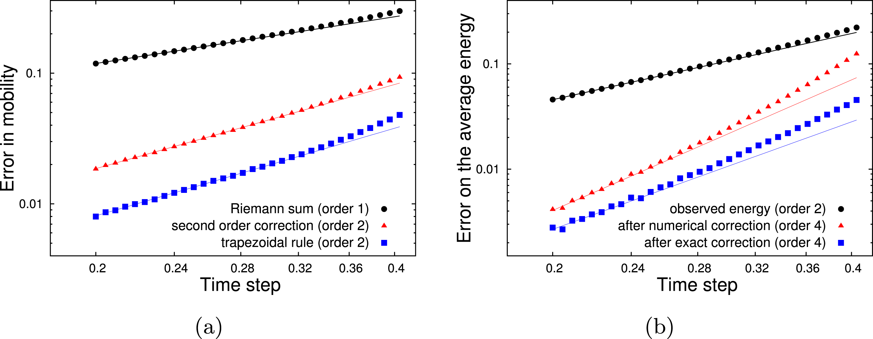
To illustrate Theorem 5.6, we consider a simple two-dimensional system with position  $q=(x,y)\in {\mathcal{M}}=(2{\it\pi}\mathbb{T})^{2}$, a potential energy function
 $V(q)=2\cos (2x)+\cos (y)$, an inverse temperature
 ${\it\beta}=1$, a friction
 ${\it\gamma}=1$ and an identity mass matrix. The external force is set to
 $F=(1,0)$. Figure 5.1
displays simulation results obtained for the scheme associated with
 $P_{{\rm\Delta}t}^{{\it\gamma}C,B,A,B,{\it\gamma}C}$ (see the discussion after (3.31) and Leimkuhler
et al. Reference Leimkuhler, Matthews and Stoltz2015) when approximating the mobility
 $$\begin{eqnarray}{\it\rho}_{F}={\it\beta}\int _{0}^{+\infty }\mathbb{E}_{{\it\mu}}(p_{t}\cdot p_{0})\,\text{d}t.\end{eqnarray}$$
For this second-order scheme, an approximation of the time
integral based on a simple Riemann sum leads to errors of order  ${\rm\Delta}t$, while a second-order convergence is obtained upon modifying the
observables according to (5.25)
or using a trapezoidal rule. In addition, we show how to improve the computation
of the average value of the Hamiltonian
 $H(q,p)=V(q)+|p|^{2}/2$ based on an estimation of the correction term (3.32) reformulated as some
integrated correlation function. In the case of the total energy, the
corresponding correction is proportional to the mobility
 ${\it\rho}_{F}$. As predicted by theoretical results similar to
Theorem 3.3, errors
in average properties can be reduced from
 ${\rm\Delta}t^{2}$ to
 ${\rm\Delta}t^{3}$ when the correction term is correctly estimated; in fact, the
errors can be shown to be reduced to order
 ${\rm\Delta}t^{4}$ (see Theorem 2.16 in Leimkuhler
et al. Reference Leimkuhler, Matthews and Stoltz2015).
5.3.2 Linear response approaches
In this part, we discuss how to approximate a transport coefficient by estimating
numerically the derivative of equilibrium averages with respect to the forcing
parameter; see (5.10). This
requires expansions of the invariant measures of numerical approximations of
non-equilibrium dynamics with respect to two small parameters: the magnitude  ${\it\eta}$ of the forcing and the time step
 ${\rm\Delta}t$. To be more concrete, we illustrate the approach on the
computation of the mobility with the perturbed Langevin dynamics (5.1). We first present numerical
schemes for this dynamics, before stating error estimates on the computation of
average properties and linear responses. The discussion here follows the
presentation of Leimkuhler et al. (Reference Leimkuhler, Matthews and Stoltz2015, Section 3), to which we
refer for further details.
We still consider splitting schemes which reduce to the schemes presented in
Section 3.3 when  ${\it\eta}=0$. Recall that
 ${\mathcal{L}}_{0}=A+B+{\it\gamma}C$, where the elementary operators
 $A,B,C$ are introduced in (3.30):
 $$\begin{eqnarray}A=M^{-1}p\cdot {\rm\nabla}_{q},\quad B=-{\rm\nabla}V(q)\cdot {\rm\nabla}_{p},\quad C=-M^{-1}p\cdot {\rm\nabla}_{p}+\frac{1}{{\it\beta}}{\rm\Delta}_{p}.\end{eqnarray}$$
Since the aim is to decompose the evolution generated by  ${\mathcal{L}}_{{\it\eta}}={\mathcal{L}}_{0}+{\it\eta}\widetilde{{\mathcal{L}}}$ into analytically integrable parts, there are two principal
options: either replace
 $B$ by
 $$\begin{eqnarray}B_{{\it\eta}}=B+{\it\eta}\widetilde{{\mathcal{L}}}\end{eqnarray}$$
or replace  ${\it\gamma}C$ by
 ${\it\gamma}C+{\it\eta}\widetilde{{\mathcal{L}}}$. However, the schemes built on the latter option do not perform
correctly in the overdamped limit, since their invariant measures are not
consistent with the invariant measures of non-equilibrium overdamped Langevin
dynamics, that is,
 $$\begin{eqnarray}\text{d}q_{t}=(-{\rm\nabla}V(q_{t})+{\it\eta}F)\,\text{d}t+\sqrt{\frac{2}{{\it\beta}}}\,\text{d}W_{t}.\end{eqnarray}$$
The latter dynamics is obtained from (5.1) in the limit  ${\it\gamma}\rightarrow +\infty$ upon rescaling the time as
 ${\it\gamma}t$. To illustrate this point, consider for instance the first-order
splitting scheme associated with the evolution operator
 $$\begin{eqnarray}P_{{\rm\Delta}t}^{A,B,{\it\gamma}C+{\it\eta}\widetilde{{\mathcal{L}}}}=\text{e}^{{\rm\Delta}t\,A}\,\text{e}^{{\rm\Delta}t\,B}\,\text{e}^{{\rm\Delta}t({\it\gamma}C+{\it\eta}\widetilde{{\mathcal{L}}})},\end{eqnarray}$$
that is,
 $$\begin{eqnarray}\displaystyle q^{n+1} & = & \displaystyle q^{n}+{\rm\Delta}t\,M^{-1}p^{n},\nonumber\\ \displaystyle \widetilde{p}^{n+1} & = & \displaystyle p^{n}-{\rm\Delta}t\,{\rm\nabla}V(q^{n+1}),\nonumber\\ \displaystyle p^{n+1} & = & \displaystyle {\it\alpha}_{{\rm\Delta}t}\widetilde{p}^{n+1}+\frac{1-{\it\alpha}_{{\rm\Delta}t}}{{\it\gamma}}\,{\it\eta}F+\sqrt{\frac{1-{\it\alpha}_{{\rm\Delta}t}^{2}}{{\it\beta}}M}\,G^{n},\nonumber\end{eqnarray}$$
where  ${\it\alpha}_{{\rm\Delta}t}=\exp (-{\it\gamma}M^{-1}{\rm\Delta}t)$ is defined after (3.31), and
 $(G^{n})$ is a sequence of i.i.d. Gaussian random vectors with
identity covariance. When
 $M=\text{Id}$ and
 ${\it\gamma}\rightarrow +\infty$, a standard Euler–Maruyama discretization of the
equilibrium overdamped Langevin dynamics (i.e.
 ${\it\eta}=0$) is obtained; whereas we would like to obtain a consistent
discretization of non-equilibrium overdamped Langevin dynamics (5.27). This suggests that numerical
methods based on the integration of
 ${\it\gamma}C+{\it\eta}\widetilde{{\mathcal{L}}}$ will not estimate the mobility for large
 ${\it\gamma}$ correctly.
We therefore prefer to consider schemes obtained by replacing  $B$ with
 $B+{\it\eta}\widetilde{{\mathcal{L}}}$, such as the first-order splitting
 $$\begin{eqnarray}P_{{\rm\Delta}t}^{A,B+{\it\eta}\widetilde{{\mathcal{L}}},{\it\gamma}C}=\text{e}^{{\rm\Delta}t\,A}\,\text{e}^{{\rm\Delta}t(B+{\it\eta}\widetilde{{\mathcal{L}}})}\,\text{e}^{{\it\gamma}{\rm\Delta}t\,C},\end{eqnarray}$$
or the second-order splitting
 $$\begin{eqnarray}P_{{\rm\Delta}t}^{{\it\gamma}C,B+{\it\eta}\widetilde{{\mathcal{L}}},A,B+{\it\eta}\widetilde{{\mathcal{L}}},{\it\gamma}C}=\text{e}^{{\it\gamma}{\rm\Delta}t\,C/2}\,\text{e}^{{\rm\Delta}t(B+{\it\eta}\widetilde{{\mathcal{L}}})/2}\,\text{e}^{{\rm\Delta}t\,A}\,\text{e}^{{\rm\Delta}t(B+{\it\eta}\widetilde{{\mathcal{L}}})/2}\,\text{e}^{{\it\gamma}{\rm\Delta}t\,C/2}.\end{eqnarray}$$
For example, the numerical scheme associated with  $P_{{\rm\Delta}t}^{A,B+{\it\eta}\widetilde{{\mathcal{L}}},{\it\gamma}C}$,
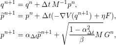 $$\begin{eqnarray}\displaystyle q^{n+1} & = & \displaystyle q^{n}+{\rm\Delta}t\,M^{-1}p^{n},\nonumber\\ \displaystyle \widetilde{p}^{n+1} & = & \displaystyle p^{n}+{\rm\Delta}t(-{\rm\nabla}V(q^{n+1})+{\it\eta}F),\nonumber\\ \displaystyle p^{n+1} & = & \displaystyle {\it\alpha}_{{\rm\Delta}t}\widetilde{p}^{n+1}+\sqrt{\frac{1-{\it\alpha}_{{\rm\Delta}t}^{2}}{{\it\beta}}M}\,G^{n},\nonumber\end{eqnarray}$$
when  $M=\text{Id}$ and in the limit as
 ${\it\gamma}\rightarrow +\infty$, is a consistent discretization of non-equilibrium Langevin
dynamics (5.27). Henceforth we
let
 $P_{{\it\eta},{\rm\Delta}t}$ denote the evolution operator associated with one of these
schemes for a fixed value of the friction
 ${\it\gamma}$ (see Remark 5.11 for a discussion of the limiting regime
 ${\it\gamma}\rightarrow +\infty$).
It can be shown that there exists a unique invariant measure  ${\it\mu}_{{\it\eta},{\rm\Delta}t}$ for the Markov chains induced by
 $P_{{\it\eta},{\rm\Delta}t}$ by following the strategy outlined in Section 2.4. The crucial point is that the gradient
structure of the force term is never used explicitly in the proofs of the Lyapunov
and minorization conditions (see Assumptions 2.23 and 2.24) since we rely solely on the boundedness of the force. This in
fact allows us to obtain exponential convergence results similar to (2.65) (Leimkuhler
et al. Reference Leimkuhler, Matthews and Stoltz2015, Proposition 3.3): for any
 ${\it\eta}_{\ast }>0$ and for any
 $s\geqslant 0$, there exist
 $C,{\it\lambda},{\rm\Delta}t^{\ast }>0$ (which depend on
 $s$ and
 ${\it\eta}_{\ast }$) such that, for all
 ${\rm\Delta}t\in (0,{\rm\Delta}t^{\ast }]$ and for all
 ${\it\eta}\in [-{\it\eta}_{\ast },{\it\eta}_{\ast }]$,
 $$\begin{eqnarray}\Vert P_{{\it\eta},{\rm\Delta}t}^{n}\Vert _{{\mathcal{B}}(L_{{\mathcal{K}}_{s},{\rm\Delta}t,{\it\eta}}^{\infty })}\leqslant C\,\text{e}^{-{\it\lambda}n{\rm\Delta}t},\quad \text{for all }n\in \mathbb{N},\end{eqnarray}$$
where
 $$\begin{eqnarray}L_{{\mathcal{K}}_{s},{\rm\Delta}t,{\it\eta}}^{\infty }({\mathcal{E}})=\biggl\{{\it\varphi}\in L_{{\mathcal{K}}_{s}}^{\infty }({\mathcal{E}})\,\bigg|\,\int _{{\mathcal{E}}}{\it\varphi}\,\text{d}{\it\mu}_{{\it\eta},{\rm\Delta}t}=0\biggr\}.\end{eqnarray}$$
Let us emphasize that we do not have any control over the
convergence rate  ${\it\lambda}$ in terms of
 ${\it\eta}^{\ast }$, and it could well be that
 ${\it\lambda}$ goes to 0 as
 ${\it\eta}^{\ast }$ increases.
The following result provides error estimates for the invariant measure of
splitting schemes such as (5.28) and (5.29) (see Theorem 3.4 in Leimkuhler
et al. (Reference Leimkuhler, Matthews and Stoltz2015)). The proof follows the same lines as the proof of
Theorem 3.3, except
that expansions are performed with respect to the two small parameters  ${\rm\Delta}t$ and
 ${\it\eta}$.
Theorem 5.9 (error estimates on the invariant measure for ${\it\eta}\neq 0$).

Set  ${\it\alpha}=1$ for first-order splitting schemes such
as (5.28)
and
 ${\it\alpha}=2$ for second-order splitting schemes such
as (5.29).
Then there exist functions
 $f_{{\it\alpha},0},f_{{\it\alpha},1}\in {\mathcal{S}}_{0}$ such that, for any smooth function
 ${\it\varphi}\in {\mathcal{S}}$, there is
 ${\rm\Delta}t^{\ast },{\it\eta}^{\ast },K>0$ (depending on
 ${\it\varphi}$) for which, for all
 ${\it\eta}\in [-{\it\eta}^{\ast },{\it\eta}^{\ast }]$ and
 ${\rm\Delta}t\in (0,{\rm\Delta}t^{\ast }]$,
 $$\begin{eqnarray}\int _{{\mathcal{E}}}{\it\varphi}\,\text{d}{\it\mu}_{{\it\eta},{\rm\Delta}t}=\int _{{\mathcal{E}}}{\it\varphi}(1+{\it\eta}f_{0,1}+{\rm\Delta}t^{{\it\alpha}}f_{{\it\alpha},0}+{\it\eta}{\rm\Delta}t^{{\it\alpha}}f_{{\it\alpha},1})\,\text{d}{\it\mu}+r_{{\it\varphi},{\it\eta},{\rm\Delta}t},\end{eqnarray}$$
where  $f_{0,1}$ is the unique solution of the Poisson equation
 $$\begin{eqnarray}{\mathcal{L}}_{0}^{\ast }f_{0,1}=-\widetilde{{\mathcal{L}}}^{\ast }\mathbf{1}=-{\it\beta}F^{T}M^{-1}p,\end{eqnarray}$$
and
 $$\begin{eqnarray}|r_{{\it\varphi},{\it\eta},{\rm\Delta}t}|\leqslant K({\it\eta}^{2}+{\rm\Delta}t^{{\it\alpha}+1}),\quad \frac{|r_{{\it\varphi},{\it\eta},{\rm\Delta}t}-r_{{\it\varphi},0,{\rm\Delta}t}|}{{\it\eta}}\leqslant K({\it\eta}+{\rm\Delta}t^{{\it\alpha}+1}).\end{eqnarray}$$
Let us now comment on (5.30). In this formula, the function  $f_{0,1}$ encodes the linear response of the invariant measure when the
perturbation is turned on for the continuous dynamics (see (5.12)), while
 $f_{{\it\alpha},0}$, to leading order, accounts for the perturbation induced by the
use of finite time steps. As shown below in Corollary 5.10, the errors on transport
coefficients are determined at leading order by the cross-term of order
 ${\it\eta}{\rm\Delta}t^{{\it\alpha}}$, which involves the correction function
 $f_{{\it\alpha},1}$. Note that the remainder term
 $r_{{\it\varphi},{\it\eta},{\rm\Delta}t}$ now collects higher-order terms both as powers of the time step
 ${\rm\Delta}t$ and the non-equilibrium parameter
 ${\it\eta}$. The estimates we obtain on the remainder, however, allow us to
take the linear response limit
 ${\it\eta}\rightarrow 0$, as made precise by the following error estimate on the
transport coefficient (which is an immediate consequence of
Theorem 5.9). In
order to state the result, we introduce the reference linear response for an
observable
 ${\it\varphi}\in {\mathcal{S}}$, namely
 $$\begin{eqnarray}\mathscr{R}_{{\it\varphi},0}=\lim _{{\it\eta}\rightarrow 0}\frac{1}{{\it\eta}}\biggl(\int _{{\mathcal{E}}}{\it\varphi}\,\text{d}{\it\mu}_{{\it\eta}}-\int _{{\mathcal{E}}}{\it\varphi}\,\text{d}{\it\mu}\biggr),\end{eqnarray}$$
and its numerical approximation,
 $$\begin{eqnarray}\mathscr{R}_{{\it\varphi},{\rm\Delta}t}=\lim _{{\it\eta}\rightarrow 0}\frac{1}{{\it\eta}}\biggl(\int _{{\mathcal{E}}}{\it\varphi}\,\text{d}{\it\mu}_{{\it\eta},{\rm\Delta}t}-\int _{{\mathcal{E}}}{\it\varphi}\,\text{d}{\it\mu}_{0,{\rm\Delta}t}\biggr).\end{eqnarray}$$
It is often the case that the observable  ${\it\varphi}$ of interest has a vanishing average with respect to
 ${\it\mu}$, as for the function
 $\widetilde{{\mathcal{L}}}^{\ast }\mathbf{1}={\it\beta}F^{T}M^{-1}p$ used to compute the mobility in (5.10). Even in such cases,
 ${\it\varphi}$ generally has a non-zero average with respect to the invariant
measure
 ${\it\mu}_{0,{\rm\Delta}t}$ of the numerical scheme associated with a discretization of the
equilibrium dynamics, so that it is indeed important to subtract the average
obtained with
 ${\it\eta}=0$ in (5.31).
Corollary 5.10 (error estimates on linear responses).
Under the assumptions of Theorem 5.9, and for any  ${\it\varphi}\in {\mathcal{S}}$, there exist
 ${\rm\Delta}t^{\ast }>0$ and a constant
 $K>0$ such that
 $$\begin{eqnarray}\mathscr{R}_{{\it\varphi},{\rm\Delta}t}=\mathscr{R}_{{\it\varphi},0}+{\rm\Delta}t^{{\it\alpha}}\int _{{\mathcal{E}}}{\it\varphi}\,f_{{\it\alpha},1}\,\text{d}{\it\mu}+{\rm\Delta}t^{{\it\alpha}+1}r_{{\it\varphi},{\rm\Delta}t},\end{eqnarray}$$
with  $|r_{{\it\varphi},{\rm\Delta}t}|\leqslant K$ when
 $0<{\rm\Delta}t\leqslant {\rm\Delta}t^{\ast }$.
Note that, in contrast with the error estimates provided by the
Green–Kubo formulae, the error is of order  ${\rm\Delta}t^{{\it\alpha}}$ without any need to modify the observable. This makes the linear
response approach more attractive than Green–Kubo techniques when
 ${\it\alpha}$ is large and the correction function (5.25) is difficult to compute.
As an application, we obtain the following estimate on the numerically computed mobility:
 $$\begin{eqnarray}\displaystyle {\it\rho}_{F,{\rm\Delta}t} & = & \displaystyle \lim _{{\it\eta}\rightarrow 0}\frac{1}{{\it\eta}}\biggl(\int _{{\mathcal{E}}}F^{T}M^{-1}p\,{\it\mu}_{{\it\eta},{\rm\Delta}t}(\text{d}q\,\text{d}p)-\int _{{\mathcal{E}}}F^{T}M^{-1}p\,{\it\mu}_{0,{\rm\Delta}t}(\text{d}q\,\text{d}p)\biggr)\nonumber\\ \displaystyle & = & \displaystyle {\it\rho}_{F}+{\rm\Delta}t^{{\it\alpha}}\int _{{\mathcal{E}}}F^{T}M^{-1}p\,f_{{\it\alpha},1}\,\text{d}{\it\mu}+{\rm\Delta}t^{{\it\alpha}+1}r_{{\rm\Delta}t},\end{eqnarray}$$
where  ${\it\rho}_{F}$ is defined in (5.10). This error estimate is illustrated in Figures 5.2 and 5.3 for the same system as in Figure 5.1. More precisely, we check in Figure 5.2 that, for a given time step
 ${\rm\Delta}t$, the average velocity in the direction
 $F$ is indeed linear with respect to
 ${\it\eta}$ for
 ${\it\eta}$ sufficiently small. The corresponding slope gives an estimate of
 ${\it\rho}_{F,{\rm\Delta}t}$. These estimates are then reported as a function of
 ${\rm\Delta}t$ in Figure 5.3.
They extrapolate to the same value at
 ${\rm\Delta}t=0$, with errors of order
 ${\rm\Delta}t$ for first-order splitting schemes, and
 ${\rm\Delta}t^{2}$ for second-order splitting schemes, as expected from
Corollary 5.10.
Linear response of the numerical approximation of the average velocity  $\mathbb{E}_{{\it\eta}}(F^{T}M^{-1}p)$ as a function of
 ${\it\eta}$ for the scheme associated with
 $P_{{\rm\Delta}t}^{{\it\gamma}C,B+{\it\eta}\widetilde{{\mathcal{L}}},A,B+{\it\eta}\widetilde{{\mathcal{L}}},{\it\gamma}C}$, for
 ${\rm\Delta}t=0.01$. A linear fit on the first ten values gives a slope of
 ${\it\rho}_{F,{\rm\Delta}t}\simeq 0.07416$.
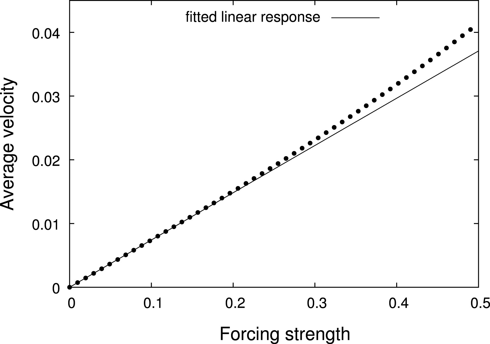
Estimated mobility  ${\it\rho}_{F,{\rm\Delta}t}$ for the first-order scheme
 $P_{{\rm\Delta}t}^{A,B+{\it\eta}\widetilde{{\mathcal{L}}},{\it\gamma}C}$ and second-order scheme
 $P_{{\rm\Delta}t}^{{\it\gamma}C,B+{\it\eta}\widetilde{{\mathcal{L}}},A,B+{\it\eta}\widetilde{{\mathcal{L}}},{\it\gamma}C}$ as a function of the time step
 ${\rm\Delta}t$. The fits give
 ${\it\rho}_{F,{\rm\Delta}t}\simeq 0.0740+0.0817{\rm\Delta}t$ and
 ${\it\rho}_{F,{\rm\Delta}t}\simeq 0.0741+0.197{\rm\Delta}t^{2}$, respectively.
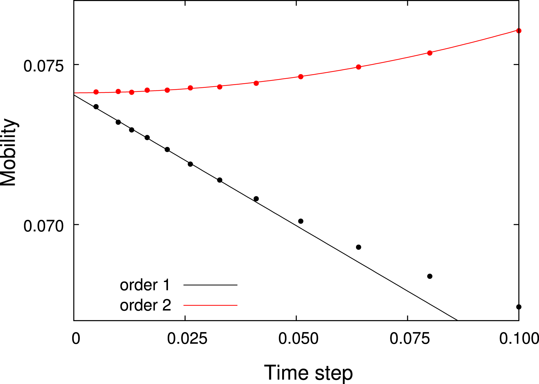
Remark 5.11 (overdamped limits).
As explained in Leimkuhler et al. (Reference Leimkuhler, Matthews and Stoltz2015, Section 3.4), it is
possible to study the overdamped limit  ${\it\gamma}\rightarrow +\infty$ in the above results, and in particular to obtain error
estimates on the invariant measure and on the linear response which hold
uniformly for
 ${\it\gamma}\geqslant 1$.
5.4 Variance reduction for non-equilibrium systems
One of the difficulties with the computation of average properties of non-equilibrium systems is that standard variance reduction techniques, such as those described in Section 3.4, cannot be used as such, as we illustrate below. We believe that finding appropriate variance reduction techniques for non-reversible dynamics is a challenging and interesting open problem.
5.4.1 Importance sampling
If the drift term  $-{\rm\nabla}V$ of equilibrium (overdamped) Langevin dynamics is modified to
 $-{\rm\nabla}(V+\widetilde{V})$, the changes in the invariant probability measure can be
explicitly written down: this measure now reads
 $\widetilde{Z}^{-1}\text{e}^{-{\it\beta}(V+\widetilde{V})(q)}\text{d}q$. On the other hand, consider non-equilibrium dynamics
 $$\begin{eqnarray}\text{d}q_{t}=b(q_{t})\,\text{d}t+\sqrt{2}\,\text{d}W_{t},\end{eqnarray}$$
with invariant measure  ${\it\psi}_{\infty }(q)\,\text{d}q$, perturbed by a gradient term, such as
 $$\begin{eqnarray}\text{d}q_{t}=(b(q_{t})+{\rm\nabla}A(q_{t}))\,\text{d}t+\sqrt{2}\,\text{d}W_{t}.\end{eqnarray}$$
We let  ${\it\psi}_{\infty }^{A}(q)\,\text{d}q$ denote the invariant measure of this process, assuming it
exists. In general,
 ${\it\psi}_{\infty }^{A}(q)\,\text{d}q$ is different from
 $Z^{-1}{\it\psi}_{\infty }(q)\text{e}^{A(q)}\,\text{d}q$ (consider for instance the simple example (5.5), for which the unique
invariant probability measure is the uniform measure on
 ${\mathcal{D}}=\mathbb{T}$ when
 $V=0$, which transforms into (5.7) when
 $V\neq 0$). The expression of
 ${\it\psi}_{\infty }^{A}$ is not known, and generally has no simple relationship with the
expression of
 ${\it\psi}_{\infty }$. It is therefore unclear how to use importance sampling
strategies for non-equilibrium systems.
5.4.2 Stratification
For equilibrium systems, it is easy to construct constrained dynamics to sample the restriction of the invariant measure of the unconstrained dynamics to some submanifold. This is the principle of thermodynamic integration, for example (see Section 4.5). The invariant measure of constrained non-equilibrium dynamics may, on the other hand, have no relationship whatsoever with the invariant measure of the unconstrained non-equilibrium dynamics. Let us illustrate this point with a simple example. Consider the dynamics
 $$\begin{eqnarray}\displaystyle \text{d}q_{1,t} & = & \displaystyle \partial _{q_{2}}U(q_{1,t},q_{2,t})+\sqrt{2}\,\text{d}W_{1,t},\nonumber\\ \displaystyle \text{d}q_{2,t} & = & \displaystyle -\partial _{q_{1}}U(q_{1,t},q_{2,t})+\sqrt{2}\,\text{d}W_{2,t},\nonumber\end{eqnarray}$$
on the state space  $\mathbb{T}^{2}$, for a given
 $C^{\infty }$ periodic function
 $U$. A simple computation shows that
 ${\it\psi}_{\infty }=\mathbf{1}_{\mathbb{T}^{2}}$ is an invariant probability measure. In addition, this is the
unique invariant probability measure since the process is irreducible. Consider
now the constraint
 ${\it\xi}(q)=0$ for the choice
 ${\it\xi}(q)=q_{2}$. On the one hand, the restriction of
 ${\it\psi}_{\infty }$ to the space
 $\{q\in \mathbb{T}^{2}\mid {\it\xi}(q)=0\}=\mathbb{T}\times \{0\}$ is
 $\overline{{\it\psi}}_{\infty }(q_{1})=\mathbf{1}_{\mathbb{T}}$. On the other hand, the process constrained using a constraining
force in the direction of
 ${\rm\nabla}{\it\xi}$ reads
 $$\begin{eqnarray}\text{d}q_{1,t}=f(q_{1,t})\,\text{d}t+\sqrt{2}\text{d}W_{1,t},\quad f(q_{1})=\partial _{q_{2}}U(q_{1},0).\end{eqnarray}$$
In general, the invariant measure for this process is different
from  $\mathbf{1}_{\mathbb{T}}$. Indeed, introduce
 $$\begin{eqnarray}F=\int _{0}^{1}f,\quad V(q_{1})=-\int _{0}^{q_{1}}(f(s)-F)\,\text{d}s.\end{eqnarray}$$
Note that  $V$ is a periodic function (
 $V(0)=V(1)=0$), and that
 $f(q_{1})=-V^{\prime }(q_{1})$. The computations performed in Section 5.1 show that the unique invariant probability
measure of the constrained process is
 $$\begin{eqnarray}{\it\psi}_{\infty }(q_{1})=Z^{-1}\int _{0}^{1}\,\text{e}^{V(q_{1}+y)-V(q_{1})-Fy}\,\text{d}y,\end{eqnarray}$$
which is different from  $\mathbf{1}_{\mathbb{T}}$ in general.
5.4.3 Control variate method
This method has been applied to non-equilibrium systems, but only for stochastic dynamics, for which the coupling between two configurations driven by the same random noise is strong – for example one-dimensional lattice gas systems (Goodman and Lin Reference Goodman and Lin2009). The general idea of the control variate method in this context is to simulate a system at equilibrium and a system subjected to a small external forcing, and to monitor the difference between the flux of interest in the non-equilibrium system, and the flux in the equilibrium one (which, up to statistical errors, should vanish). When the coupling is sufficiently strong, the variance of the difference of the fluxes is much smaller than the variance of the flux of the non-equilibrium system alone. On the other hand, this approach is very difficult to use in systems where the coupling is too weak, such as perturbations of Hamiltonian dynamics, or overdamped Langevin dynamics in regions where the Hessian of the potential is not positive definite. With some care, however, it is possible to estimate finite time correlation functions, as done by Ciccotti and Jacucci (Reference Ciccotti and Jacucci1975).
An interesting question is: Is there a way to modify the dynamics in order to increase its coupling properties, while keeping the value of the linear response of the observable of interest fixed? This is, to the best of our knowledge, an open problem.
Remark 5.12 (adding non-reversible drifts).
Non-reversible dynamics can also be obtained by perturbing reversible
dynamics with a non-gradient force, which is divergence-free with respect to
the equilibrium measure, however, and hence does not modify the invariant
measure under consideration. At variance with the situations discussed
above, where the non-reversible drift in the dynamics is fixed by the
physical problem at hand (the computation of a given transport coefficient,
induced for instance by the constant force  ${\it\eta}F$ in (5.1)) and the non-equilibrium steady state is unknown, here the
non-equilibrium steady state is fixed and equal to the equilibrium measure
of the reversible dynamics under consideration. Moreover, the non-reversible
drift is chosen by the user in order to accelerate the
sampling procedure. For overdamped Langevin dynamics, there are several
results confirming that the addition of non-gradient but divergence-free
drifts improves the sampling, measured either in terms of convergence of the
law of the process to the invariant distribution or in terms of asymptotic
variance of observables of interest. In fact, both criteria are related to
spectral gap estimates. For further precision we refer to Hwang, Hwang-Ma
and Sheu Reference Hwang, Hwang-Ma and Sheu1993, Reference Hwang, Hwang-Ma and Sheu2005 Lelièvre, Nier and
Pavliotis (Reference Lelièvre, Nier and Pavliotis2013), Duncan
et al. (Reference Duncan, Lelièvre and Pavliotis2016) and Rey-Bellet and Spiliopoulos Reference Rey-Bellet and Spiliopoulos2015, Reference Rey-Bellet and Spiliopoulos2016, for
example.
6 Computing dynamical quantities: path sampling and accelerated dynamics
In this section we discuss the computation of dynamical quantities, namely average properties over trajectories of Langevin or overdamped Langevin dynamics (1.9) and (1.8). As already explained above (see in particular Section 1.2), the main difficulty when computing average properties with such dynamics is metastability: the trajectories remain trapped for very long times in some metastable states. This means that behind the continuous state-space dynamics (1.9) or (1.8), there is a discrete state-space Markov process encoding the jumps from one metastable state to another. This has already been mentioned in Section 2.5 and is discussed at length in Section 6.3. Discrete state-space Markov dynamics are also very prevalent in molecular dynamics: these are called kinetic Monte Carlo or Markov state models (see for example Voter Reference Voter, Sickafus, Kotomin and Uberuaga2007). Continuous state-space models are then typically used to parametrize these Markovian models, that is, to compute the jump rates between metastable states, using Arrhenius (or Eyring–Kramers) formulae, for example (see (2.83)).
We will present some techniques to efficiently sample the exit event from a metastable state, or the reactive path between metastable states. In Section 6.1 we first introduce a preliminary tool, to be used many times thereafter, namely the Feynman–Kac formula, which we immediately illustrate with a simple application: the Jarzynski identity (which we already mentioned briefly in Section 4.5). We then present two ideas which have been followed to efficiently sample metastable paths: importance sampling approaches on path space, using control problems to build good importance functions (see Section 6.2), and the notion of quasi-stationary distributions (QSDs), to analyse the exit event from a metastable state (see Section 6.3). Finally, in Section 6.4, we present accelerated dynamics techniques, which were introduced by A. F. Voter in the late 1990s, and which can be analysed using the framework introduced in Section 6.3.
Let us finally make two preliminary remarks before embarking on the details. First, as explained in Sections 3 and 4, computing thermodynamic quantities (i.e. sampling the canonical measure) is a fairly well understood problem, with many techniques available that are used in many other scientific fields (e.g. computational statistics and uncertainty quantification). In contrast, the computation of dynamical properties is a numerical challenge that has been less explored by applied mathematicians, probably because it is more specific to molecular dynamic simulations. Many techniques are available, and this is a very lively subject with new methods appearing at a rapid pace. We will devote Section 6.5 to an overview of such techniques, to the best of our current knowledge. The second remark is more technical. In this section we mainly focus on overdamped Langevin dynamics (1.8) when presenting mathematical results, but the reader should bear in mind that the algorithms presented apply equally to Langevin dynamics (1.9). We will comment below on the mathematical questions raised by the extensions of the proofs to Langevin dynamics.
6.1 Feynman–Kac formula and the Jarzynski identity
6.1.1 Feynman–Kac formula
In this subsection we introduce the Feynman–Kac formula which, together with the Fokker–Planck equation presented in Section 2.1, is the second natural way to associate a partial differential equation with a stochastic differential equation. It is a generalization of formula (2.8).
Let us consider a general stochastic process  $(x_{t})_{t\geqslant 0}$ in
 $\mathbb{R}^{d}$ satisfying the stochastic differential equation (1.11). Let us recall that we let
 ${\mathcal{L}}$ denote the associated infinitesimal generator (see (1.12)).
Proposition 6.1. Let  $S$ be a
 $C^{\infty }$ bounded domain of
 $\mathbb{R}^{d}$, and let
 $f:S\rightarrow \mathbb{R}^{d}$,
 $v_{0}:S\rightarrow \mathbb{R}^{d}$ and
 ${\it\varphi}:\partial S\rightarrow \mathbb{R}$ be three
 $C^{\infty }$ functions. Let
 $v(t,y)$ be a smooth solution (
 $C^{1}$ in
 $t$ and
 $C^{2}$ in
 $y$ is sufficient) to the boundary value problem:
 $$\begin{eqnarray}\begin{array}{@{}rcll@{}}\partial _{t}v\ & =\ & {\mathcal{L}}v+fv\quad & \text{for }t\geqslant 0,\;y\in S,\\ v\ & =\ & {\it\varphi}\quad & \text{on }\partial S,\\ v(0,y)\ & =v_{0}(y).~\end{array}\end{eqnarray}$$
Then,
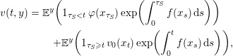 $$\begin{eqnarray}\displaystyle v(t,y) & = & \displaystyle \mathbb{E}^{y}\biggl(1_{{\it\tau}_{S}<t}\,{\it\varphi}(x_{{\it\tau}_{S}})\exp \biggl(\int _{0}^{{\it\tau}_{S}}f(x_{s})\,\text{d}s\biggr)\biggr)\nonumber\\ \displaystyle & & \displaystyle \quad +\mathbb{E}^{y}\biggl(1_{{\it\tau}_{S}\geqslant t}\,v_{0}(x_{t})\exp \biggl(\int _{0}^{t}f(x_{s})\,\text{d}s\biggr)\biggr),\end{eqnarray}$$
where  $(x_{t})_{t\geqslant 0}$ is the process satisfying (1.11),
 ${\it\tau}_{S}$ is the first exit time of
 $(x_{t})_{t\geqslant 0}$ from
 $S$,
 $$\begin{eqnarray}{\it\tau}_{S}=\inf \{t\geqslant 0,x_{t}\not \in S\},\end{eqnarray}$$
and the superscript  $y$ in the notation
 $\mathbb{E}^{y}$ indicates that the initial condition is
 $x_{0}=y\in \mathbb{R}^{d}$.
Let us emphasize that (6.1) is a representation formula: it gives a probabilistic representation to a smooth solution of the PDE, but does not say anything as such about the existence or the regularity of this solution.
Proof. Fix a time  $t>0$ and consider
 $u(s,y)=v(t-s,y)$ for
 $s\in [0,t]$. The function
 $u$ satisfies
 $$\begin{eqnarray}\begin{array}{@{}rcll@{}}\partial _{s}u+{\mathcal{L}}u+fu\ & =\ & 0\quad & \text{for }s\in [0,t],\;y\in S,\\ u\ & =\ & {\it\varphi}\quad & \text{on }\partial S,\\ u(t,y)\ & =\ & v_{0}(y).\quad & \end{array}\end{eqnarray}$$
Using Itô calculus,  $\text{for all }s\in [0,\min ({\it\tau}_{S},t)]$ we obtain
 $$\begin{eqnarray}\displaystyle & & \displaystyle u(s,x_{s})\exp \biggl(\int _{0}^{s}f(x_{r})\,\text{d}r\biggr)\nonumber\\ \displaystyle & & \displaystyle \qquad =u(0,x_{0})+\int _{0}^{s}(\partial _{r}u+{\mathcal{L}}u+fu)(r,x_{r})\exp \biggl(\int _{0}^{r}f(x_{{\it\rho}})\,\text{d}{\it\rho}\biggr)\,\text{d}r\nonumber\\ \displaystyle & & \displaystyle \qquad \qquad +\sqrt{2{\it\beta}^{-1}}\int _{0}^{s}\exp \biggl(\int _{0}^{r}f(x_{{\it\rho}})\,\text{d}{\it\rho}\biggr){\rm\nabla}u(r,x_{r})\cdot {\it\sigma}(x_{r})\,\text{d}W_{r}\nonumber\\ \displaystyle & & \displaystyle \qquad =u(0,y)+M_{s},\nonumber\end{eqnarray}$$
where
 $$\begin{eqnarray}M_{s}=\sqrt{2{\it\beta}^{-1}}\int _{0}^{s}\exp \biggl(\int _{0}^{r}f(x_{{\it\rho}})\,\text{d}{\it\rho}\biggr){\rm\nabla}u(r,x_{r})\cdot {\it\sigma}(x_{r})\,\text{d}W_{r}\end{eqnarray}$$
is a local martingale. Since  $u$ and
 $f$ are assumed to be
 $C^{\infty }$, and
 $x_{r}$ lives in the bounded domain
 $S$ up to time
 $\min ({\it\tau}_{S},t)$, we conclude that
 $$\begin{eqnarray}\displaystyle v(t,y) & = & \displaystyle u(0,y)=\mathbb{E}^{y}\biggl(u(\min (t,{\it\tau}_{S}),x_{\min (t,{\it\tau}_{S})})\exp \biggl(\int _{0}^{\min (t,{\it\tau}_{S})}f(x_{r})\,\text{d}r\biggr)\biggr)\nonumber\\ \displaystyle & = & \displaystyle \mathbb{E}^{y}\biggl(1_{{\it\tau}_{S}<t}\,u({\it\tau}_{S},x_{{\it\tau}_{S}})\exp \biggl(\int _{0}^{{\it\tau}_{S}}f(x_{r})\,\text{d}r\biggr)\biggr)\nonumber\\ \displaystyle & & \displaystyle \quad +\mathbb{E}^{y}\biggl(1_{{\it\tau}_{S}\geqslant t}\,u(t,x_{t})\exp \biggl(\int _{0}^{t}f(x_{r})\,\text{d}r\biggr)\biggr)\nonumber\\ \displaystyle & = & \displaystyle \mathbb{E}\biggl(1_{{\it\tau}_{S}<t}\,{\it\varphi}(x_{{\it\tau}_{S}})\exp \biggl(\int _{0}^{{\it\tau}_{S}}f(x_{r})\,\text{d}r\biggr)\biggr)\nonumber\\ \displaystyle & & \displaystyle \quad +\mathbb{E}\biggl(1_{{\it\tau}_{S}\geqslant t}\,v_{0}(x_{t})\exp \biggl(\int _{0}^{t}f(x_{r})\,\text{d}r\biggr)\biggr).\nonumber\end{eqnarray}$$
This concludes the proof of (6.1).
We have presented the Feynman–Kac formula in a specific setting and under strong regularity assumptions. Many extensions exist; see for example Friedman (Reference Friedman1975, Section 6) for a general introduction and the recent work by Le Bris and Lions (Reference Le Bris and Lions2008) for generalizations to non-smooth data.
6.1.2 Jarzynski identity
Let us now present the Jarzynski identity (Jarzynski Reference Jarzynski1997), which is not a method for computing dynamical
quantities but a free energy computation technique, like the adaptive importance
sampling methods presented in Section 4. This method is described in this section since it is a simple
application of the Feynman–Kac formula. For simplicity, we present it
in the so-called alchemical setting, where the free energy is indexed by an
external parameter  ${\it\lambda}$ rather than by the value of the reaction coordinate (as in
Section 4.1). For extensions
to the reaction coordinate case, we refer for example to Lelièvre
et al. (Reference Lelièvre, Rousset and Stoltz2010, Chapter 5) and to Lelièvre
et al. (Reference Lelièvre, Rousset and Stoltz2012).
Let us assume that the potential energy  $V$ is indexed by a parameter
 ${\it\lambda}\in [0,1]$, and that
 $({\it\lambda},q)\mapsto V_{{\it\lambda}}(q)$ is
 $C^{1}$ in
 ${\it\lambda}$ and
 $C^{\infty }$ in
 $q$. Typically, one could think of the situation
 $V_{{\it\lambda}}(q)={\it\lambda}V_{1}(q)+(1-{\it\lambda})V_{0}(q)$, where
 $V_{0}$ and
 $V_{1}$ are associated with two different models. For example,
 $V_{0}$ is a potential for a homogeneous system with
 $N$ particles, and
 $V_{1}$ is the equivalent potential but for
 $N+1$ particles. Going from
 ${\it\lambda}=0$ to
 ${\it\lambda}=1$ is thus equivalent to inserting one particle in a bath of
 $N$ particles – a process known in the physics and
chemistry literature as Widom insertion (Widom Reference Widom1963). Since this process needs not be physical, we can simulate
extraordinary chemical operations such as the change of lead into gold, which
explains the name ‘alchemical setting’.
The free energy change associated with the transformation from  $V_{0}$ to
 $V_{{\it\lambda}}$ is defined as
 $$\begin{eqnarray}F({\it\lambda})-F(0)=-{\it\beta}^{-1}\ln \biggl(\displaystyle \frac{Z_{{\it\lambda}}}{Z_{0}}\biggr)\end{eqnarray}$$
(similar to the formula (4.5) in the reaction coordinate case), where for any  ${\it\lambda}\in [0,1]$,
 $$\begin{eqnarray}Z_{{\it\lambda}}=\int _{{\mathcal{D}}}\exp (-{\it\beta}V_{{\it\lambda}}).\end{eqnarray}$$
Let us explain how the Jarzynski identity can be used to compute
this quantity. The idea is to introduce a  $C^{1}$ schedule
 ${\rm\Lambda}:[0,T]\rightarrow [0,1]$ such that
 $$\begin{eqnarray}{\rm\Lambda}(0)=0,\end{eqnarray}$$
and then to simulate the non-homogeneous-in-time stochastic process
 $$\begin{eqnarray}\text{d}q_{t}=-{\rm\nabla}V_{{\rm\Lambda}(t)}(q_{t})\,\text{d}t+\sqrt{2{\it\beta}^{-1}}\,\text{d}W_{t}\end{eqnarray}$$
with an initial condition  $q_{0}$ distributed according to the probability measure
 $Z_{0}^{-1}\exp (-{\it\beta}V_{0}(q))\,\text{d}q$. We associate with each trajectory a weight defined by
 $$\begin{eqnarray}{\mathcal{W}}_{t}=\int _{0}^{t}\partial _{{\it\lambda}}V_{{\rm\Lambda}(s)}(q_{s})\dot{{\rm\Lambda}}(s)\,\text{d}s,\end{eqnarray}$$
where  $\dot{{\rm\Lambda}}$ is the time derivative of
 ${\rm\Lambda}$. Intuitively, the weight
 ${\mathcal{W}}_{t}$ represents the work associated with the alchemical process up to
time
 $t$. Then we have the following interesting result.
Proposition 6.2. Assume that  $(q_{t})_{t\geqslant 0}$ satisfies (6.2) with
 $q_{0}$ distributed according to the probability measure
 $Z_{0}^{-1}\exp (-{\it\beta}V_{0}(q))\,\text{d}q$. Then, for any time
 $t\in [0,T]$,
 $$\begin{eqnarray}\mathbb{E}[\exp (-{\it\beta}{\mathcal{W}}_{t})]=\exp [-{\it\beta}(F({\rm\Lambda}(t))-F(0))],\end{eqnarray}$$
where  ${\mathcal{W}}_{t}$ is defined by (6.3).
This formula is called the Jarzynski identity. It shows that one can recover an
equilibrium quantity (the free energy difference  $F({\rm\Lambda}(t))-F(0)$) from non-equilibrium simulations
(i.e. the non-homogeneous-in-time dynamics (6.2)) started at equilibrium. In
many cases of interest, only the free energy difference
 $F(1)-F(0)$ associated with the transformation from
 $V_{0}$ to
 $V_{1}$ is of interest: one then chooses
 ${\rm\Lambda}$ such that
 ${\rm\Lambda}(T)=1$, and the free energy difference is given by
 $F(1)-F(0)=-{\it\beta}^{-1}\ln (\mathbb{E}[\exp (-{\it\beta}{\mathcal{W}}_{T})])$.
Proof. The proof is based on a Feynman–Kac formula in the spirit of
(6.1) but adapted to
the non-homogeneous-in-time setting. Indeed, for a fixed time  $t$, let us consider a
 $C^{\infty }$ solution
 $v:[0,t]\times {\mathcal{D}}\rightarrow \mathbb{R}$ to the backward-in-time partial differential equation
 $$\begin{eqnarray}\begin{array}{@{}rcll@{}}\partial _{s}v(s,x)\ & =\ & -{\mathcal{L}}_{s}v(s,x)+{\it\beta}\partial _{{\it\lambda}}V_{{\rm\Lambda}(s)}(x)\dot{{\rm\Lambda}}(s)v(s,x)\quad & \text{for }(s,x)\in [0,t]\times {\mathcal{D}},\\ v(t,x)\ & =\ & f(x)\quad & \text{for }x\in {\mathcal{D}},\end{array}\end{eqnarray}$$
where  ${\mathcal{L}}_{s}=-{\rm\nabla}V_{{\rm\Lambda}(s)}\cdot {\rm\nabla}+{\it\beta}^{-1}{\rm\Delta}$ is the infinitesimal generator of (6.2). This is a standard
parabolic equation which admits a unique
 $C^{\infty }$ solution under standard regularity assumptions on the
coefficients, the domain
 ${\mathcal{D}}$ and the function
 $f$. The Feynman–Kac formula in this context is
given by
 $$\begin{eqnarray}v(s,x)=\mathbb{E}^{s,x}(f(q_{t})\,\text{e}^{-{\it\beta}({\mathcal{W}}_{t}-{\mathcal{W}}_{s})}),\end{eqnarray}$$
where the superscript  $s,x$ indicates that one considers the solution to (6.2) for
 $t\geqslant s$ with initial condition
 $q_{s}=x$. The proof of (6.5) is very similar to the proof of (6.1). Indeed, using
Itô calculus over the time interval
 $[s,t]$, one obtains
 $$\begin{eqnarray}\displaystyle & & \displaystyle v(t,q_{t})\exp \biggl(-{\it\beta}\int _{s}^{t}\partial _{{\it\lambda}}V_{{\rm\Lambda}({\it\rho})}(q_{{\it\rho}})\dot{{\rm\Lambda}}({\it\rho})\,\text{d}{\it\rho}\biggr)=v(s,q_{s})\nonumber\\ \displaystyle & & \displaystyle \qquad +\sqrt{2{\it\beta}^{-1}}\int _{s}^{t}\exp \biggl(-{\it\beta}\int _{s}^{r}\partial _{{\it\lambda}}V_{{\rm\Lambda}({\it\rho})}(q_{{\it\rho}})\dot{{\rm\Lambda}}({\it\rho})\,\text{d}{\it\rho}\biggr){\rm\nabla}v(r,q_{r})\cdot \,\text{d}W_{r}\nonumber\end{eqnarray}$$
where we have used the partial differential equation
satisfied by  $v$ to cancel the bounded variation part in the Itô
formula. Equation (6.5)
then immediately follows by taking the expectation
 $\mathbb{E}^{s,x}$.
Now, it is easy to check that for any  $s\in [0,t]$,
 $$\begin{eqnarray}\frac{\text{d}}{\text{d}s}\biggl(\int _{{\mathcal{D}}}v(s,x)\exp (-{\it\beta}V_{{\rm\Lambda}(s)}(x))\,\text{d}x\biggr)=0.\end{eqnarray}$$
Indeed, using the partial differential equation satisfied by  $v$,
 $$\begin{eqnarray}\displaystyle & & \displaystyle \frac{\text{d}}{\text{d}s}\biggl(\int _{{\mathcal{D}}}v(s,x)\exp (-{\it\beta}V_{{\rm\Lambda}(s)}(x))\,\text{d}x\biggr)\nonumber\\ \displaystyle & & \displaystyle \qquad =\int _{{\mathcal{D}}}(\partial _{s}v(s,x)-{\it\beta}\partial _{{\it\lambda}}V_{{\rm\Lambda}(s)}(x)\dot{{\rm\Lambda}}(s)v(s,x))\exp (-{\it\beta}V_{{\rm\Lambda}(s)}(x))\,\text{d}x\nonumber\\ \displaystyle & & \displaystyle \qquad =-\int _{{\mathcal{D}}}{\mathcal{L}}_{s}v(s,x)\exp (-{\it\beta}V_{{\rm\Lambda}(s)}(x))\,\text{d}x=0,\nonumber\end{eqnarray}$$
where the last equality is a consequence of the invariance of the canonical measure (see (1.17)). As a consequence of (6.6), we have
 $$\begin{eqnarray}\int _{{\mathcal{D}}}v(t,x)\exp (-{\it\beta}V_{{\rm\Lambda}(t)}(x))\,\text{d}x=\int _{{\mathcal{D}}}v(0,x)\exp (-{\it\beta}V_{{\rm\Lambda}(0)}(x))\,\text{d}x.\end{eqnarray}$$
Using (6.5), this equality can be rewritten as
 $$\begin{eqnarray}\displaystyle & & \displaystyle \frac{Z_{{\rm\Lambda}(t)}}{Z_{0}}\int _{{\mathcal{D}}}f(x)Z_{{\rm\Lambda}(t)}^{-1}\exp (-{\it\beta}V_{{\rm\Lambda}(t)}(x))\,\text{d}x\nonumber\\ \displaystyle & & \displaystyle \qquad =\int _{{\mathcal{D}}}\mathbb{E}^{0,x}[f(q_{t})\exp (-{\it\beta}{\mathcal{W}}_{t})]Z_{0}^{-1}\exp (-{\it\beta}V_{{\rm\Lambda}(0)}(x))\,\text{d}x.\nonumber\end{eqnarray}$$
Taking  $f=1$, the left-hand side is
 $\exp (-{\it\beta}(F({\rm\Lambda}(t))-F(0)))$ and the right-hand side is (using a conditioning argument
on initial conditions)
 $\mathbb{E}(\exp (-{\it\beta}{\mathcal{W}}_{t}))$, where the weight
 ${\mathcal{W}}_{t}$ is computed using the solution
 $(q_{t})_{t\geqslant 0}$ to (6.2)
with initial conditions
 $q_{0}$ distributed according to the probability measure
 $Z_{0}^{-1}\exp (-{\it\beta}V_{{\rm\Lambda}(0)}(x))\,\text{d}x$. This concludes the proof of (6.4).
The Jarzynski identity is mainly useful for extracting free energy differences from experimental measurements, by performing many non-equilibrium externally driven experiments between two states of interest (Hummer and Szabo Reference Hummer and Szabo2001).
There are many extensions to this identity: generalization to other dynamics (Langevin, Hamiltonian, Nosé–Hoover dynamics), computation of free energy differences associated with a reaction coordinate (with driven constrained processes), and combination of forward-in-time and backward-in-time schedules (Jarzynski–Crooks identity). We refer to Lelièvre et al. (Reference Lelièvre, Rousset and Stoltz2010, Chapter 5) for a more comprehensive presentation.
6.2 Importance sampling on path space and Hamilton–Jacobi equations
In this section we present ideas that were developed in order to construct optimal importance sampling functions for some observables which are functions of the path of the stochastic process. This can be seen as an extension of importance sampling for canonical averages, as presented in Section 3.4.3. In this setting, partial differential equations (and in particular Hamilton–Jacobi equations) play a crucial role.
6.2.1 General setting
We consider overdamped Langevin dynamics (1.8), which we recall for convenience:
 $$\begin{eqnarray}\text{d}q_{t}=-{\rm\nabla}V(q_{t})\,\text{d}t+\sqrt{2{\it\beta}^{-1}}\text{d}W_{t}.\end{eqnarray}$$
In this section we assume for simplicity that the initial
condition is deterministic:  $q_{0}=x_{0}$ for a fixed
 $x_{0}\in {\mathcal{D}}$. Assume that the observable of interest is
 $$\begin{eqnarray}I=\mathbb{E}\biggl[\exp \biggl(g(q_{{\it\tau}})+\int _{0}^{{\it\tau}}f(q_{s})\,\text{d}s\biggr)\biggr]\end{eqnarray}$$
for given functions  $f:{\mathcal{D}}\rightarrow \mathbb{R}$ and
 $g:{\mathcal{D}}\rightarrow \mathbb{R}$ and a stopping time
 ${\it\tau}$, defined by
 $$\begin{eqnarray}{\it\tau}=\inf \{t\geqslant 0,\,q_{t}\in D\},\end{eqnarray}$$
where  $D\subset {\mathcal{D}}$ is a given domain. Let us give two examples.
∙ One could think of
$D=S^{c}$, the complement of a bounded set $S$. Then, when $f=0$, (6.7) is the average of the test function $\exp (g)$ with respect to the first exit point probability on $\partial S$ (which thus characterizes the exit point distribution
by varying $g$). When $g=0$ and $f={\it\lambda}$, (6.7) is $\mathbb{E}(\exp ({\it\lambda}{\it\tau}))$, where ${\it\tau}$ is the exit time from $S$, which thus gives the moment generating function of ${\it\tau}$. Computing (6.7) is thus important in understanding the exit event from $S$ (see Section 6.3 for more discussion of the exit event from a state $S$).∙ Another exampleFootnote 17 is
$D=A\cup B$, where $A$ and $B$ are two metastable states, $f=0$ and $\exp (g)=1_{B}$, in which case (6.7) is the probability of reaching $B$ before $A$. Trajectories starting from $x_{0}$ close to $A$ and which reach $B$ before $A$ are called reactive trajectories (Hummer Reference Hummer2004, E and Vanden-Eijnden Reference E and Vanden-Eijnden2004, Lu and Nolen Reference Lu and Nolen2015) and are important to sample in
order to identify the transition states between $A$ and $B$, for example.


Typically, approximating  $I$ by an empirical average
 $$\begin{eqnarray}\frac{1}{N}\mathop{\sum }_{n=1}^{N}\hat{I} _{n},\end{eqnarray}$$
where  $\hat{I} _{n}$ are independent realizations of the random variable
 $$\begin{eqnarray}\hat{I} =\exp \biggl(g(q_{{\it\tau}})+\int _{0}^{{\it\tau}}f(q_{s})\,\text{d}s\biggr),\end{eqnarray}$$
yields a large statistical error since
 $$\begin{eqnarray}\sqrt{\frac{\text{Var}(\hat{I} )}{I^{2}}}\end{eqnarray}$$
is large. For instance, in the second example above,  $I$ is the probability of reaching
 $B$ before
 $A$, which is very small, so the relative error
 $$\begin{eqnarray}\sqrt{\frac{\text{Var}(\hat{I} )}{I^{2}}}=\sqrt{\frac{I(1-I)}{I^{2}}}\end{eqnarray}$$
is large. We would therefore like to apply an importance sampling
procedure to reduce the variance in the estimation of  $I$.
6.2.2 Biased dynamics
Let us assume that we consider the biased dynamics
 $$\begin{eqnarray}\text{d}\tilde{q}_{t}=-{\rm\nabla}(V+\widetilde{V})(\tilde{q}_{t})\,\text{d}t+\sqrt{2{\it\beta}^{-1}}\,\text{d}W_{t},\end{eqnarray}$$
as for classical importance sampling (see (3.36)). Here  $\widetilde{V}:{\mathcal{D}}\rightarrow \mathbb{R}$ is a
 $C^{\infty }$ biasing potential. We assume that
 $\tilde{q}_{0}=q_{0}=x_{0}$. Using the Girsanov theorem (see for example Revuz and Yor Reference Revuz and Yor1999, Chapter VIII), one can show
thatFootnote 18
 $$\begin{eqnarray}I=\mathbb{E}[\hat{I} _{\widetilde{V}}],\end{eqnarray}$$
where
 $$\begin{eqnarray}\displaystyle \hat{I} _{\widetilde{V}} & = & \displaystyle \exp \biggl(g(\tilde{q}_{\tilde{{\it\tau}}})+\int _{0}^{\tilde{{\it\tau}}}f(\tilde{q}_{s})\,\text{d}s\biggr)\nonumber\\ \displaystyle & & \displaystyle \quad \times \exp \biggl(\int _{0}^{\tilde{{\it\tau}}}\frac{1}{\sqrt{2{\it\beta}^{-1}}}{\rm\nabla}\widetilde{V}(\tilde{q}_{s})\cdot \,\text{d}W_{s}-\frac{1}{2}\int _{0}^{\tilde{{\it\tau}}}\frac{1}{2{\it\beta}^{-1}}|{\rm\nabla}\widetilde{V}|^{2}(\tilde{q}_{s})\,\text{d}s\biggr),\end{eqnarray}$$
where  $\tilde{{\it\tau}}$ is now the first hitting time of
 $D$ for
 $(\tilde{q}_{t})_{t\geqslant 0}$. This is the equivalent of the unbiasing formula (3.37) on path space: the Girsanov
formula gives the change of measure so that averages with respect to the law
 $(q_{t})_{0\leqslant t\leqslant {\it\tau}}$ can be obtained from weighted averages with respect to the law
of
 $(\tilde{q}_{t})_{0\leqslant t\leqslant \tilde{{\it\tau}}}$. Using Itô calculus, we have
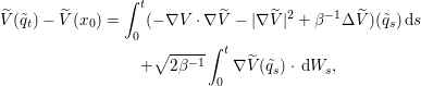 $$\begin{eqnarray}\displaystyle \widetilde{V}(\tilde{q}_{t})-\widetilde{V}(x_{0}) & = & \displaystyle \int _{0}^{t}(-{\rm\nabla}V\cdot {\rm\nabla}\widetilde{V}-|{\rm\nabla}\widetilde{V}|^{2}+{\it\beta}^{-1}{\rm\Delta}\widetilde{V})(\tilde{q}_{s})\,\text{d}s\nonumber\\ \displaystyle & & \displaystyle \quad +\sqrt{2{\it\beta}^{-1}}\int _{0}^{t}{\rm\nabla}\widetilde{V}(\tilde{q}_{s})\cdot \,\text{d}W_{s},\end{eqnarray}$$
which, once inserted in (6.10), yields
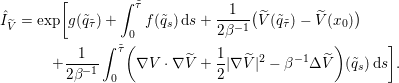 $$\begin{eqnarray}\displaystyle \hat{I} _{\widetilde{V}} & = & \displaystyle \exp \biggl[g(\tilde{q}_{\tilde{{\it\tau}}})+\int _{0}^{\tilde{{\it\tau}}}f(\tilde{q}_{s})\,\text{d}s+\displaystyle \frac{1}{2{\it\beta}^{-1}}(\widetilde{V}(\tilde{q}_{\tilde{{\it\tau}}})-\widetilde{V}(x_{0}))\nonumber\\ \displaystyle & & \displaystyle \quad +\displaystyle \frac{1}{2{\it\beta}^{-1}}\int _{0}^{\tilde{{\it\tau}}}\biggl({\rm\nabla}V\cdot {\rm\nabla}\widetilde{V}+\frac{1}{2}|{\rm\nabla}\widetilde{V}|^{2}-{\it\beta}^{-1}{\rm\Delta}\widetilde{V}\biggr)(\tilde{q}_{s})\,\text{d}s\biggr].\end{eqnarray}$$
The aim is now to build a good biasing potential  $\widetilde{V}$ such that
 $\text{Var}(\hat{I} _{\widetilde{V}})\ll \text{Var}(\hat{I} )$. Let us consider
 $$\begin{eqnarray}\widetilde{V}=-2{\it\beta}^{-1}\ln u,\end{eqnarray}$$
where, for  $x\in D^{c}$,
 $$\begin{eqnarray}u(x)=\mathbb{E}^{x}\biggl[\exp \biggl(g(q_{{\it\tau}})+\int _{0}^{{\it\tau}}f(q_{s})\,\text{d}s\biggr)\biggr].\end{eqnarray}$$
We recall that  $(q_{t})_{t\geqslant 0}$ satisfies overdamped Langevin dynamics (1.8) and that the superscript
 $x$ in
 $\mathbb{E}^{x}$ indicates that
 $q_{0}=x$. Notice in particular that
 $I=u(x_{0})$. From Proposition 6.1 (formally consider the limit
 $t\rightarrow \infty$ in (6.1)), the
function
 $u:D^{c}\rightarrow \mathbb{R}$ satisfies the partial differential equation
 $$\begin{eqnarray}\begin{array}{@{}rcll@{}}{\mathcal{L}}u+fu\ & =\ & 0\quad & \text{in }D^{c},\\ u\ & =\ & \exp (g)\quad & \text{on }\partial D,\end{array}\end{eqnarray}$$
where  ${\mathcal{L}}=-{\rm\nabla}V\cdot {\rm\nabla}+{\it\beta}^{-1}{\rm\Delta}$ is the infinitesimal generator of overdamped Langevin dynamics
introduced in (1.13). Therefore
 $\widetilde{V}=-2{\it\beta}^{-1}\ln u$ satisfies
 $$\begin{eqnarray}\begin{array}{@{}ll@{}}{\rm\nabla}V\cdot {\rm\nabla}\widetilde{V}-{\it\beta}^{-1}{\rm\Delta}\widetilde{V}+\frac{1}{2}|{\rm\nabla}\widetilde{V}|^{2}+2{\it\beta}^{-1}f=0\quad & \text{in }D^{c},\\ \widetilde{V}=-2{\it\beta}^{-1}g\quad & \text{on }\partial D\end{array}\end{eqnarray}$$
(this is the celebrated Cole–Hopf transformation).
Using  $\widetilde{V}=-2{\it\beta}^{-1}\ln u$ as a biasing potential, one thus obtains from (6.12)
 $$\begin{eqnarray}\displaystyle \hat{I} _{\widetilde{V}} & = & \displaystyle \exp \biggl(g(\tilde{q}_{\tilde{{\it\tau}}})+\frac{1}{2{\it\beta}^{-1}}(\widetilde{V}(\tilde{q}_{\tilde{{\it\tau}}})-\widetilde{V}(x_{0}))\biggr)\nonumber\\ \displaystyle & = & \displaystyle \exp \biggl(-\frac{1}{2{\it\beta}^{-1}}\widetilde{V}(x_{0})\biggr)=u(x_{0})=I.\end{eqnarray}$$
Let us summarize this discussion in a lemma.
Lemma 6.3. Consider the random variable  $\hat{I} _{\widetilde{V}}$ defined by (6.12), built using the biased dynamics (6.9). This random variable is
an unbiased estimator of
 $I$ (defined by (6.7)):
 $$\begin{eqnarray}\mathbb{E}(\hat{I} _{\widetilde{V}})=I.\end{eqnarray}$$
Moreover, let us assume that the biasing potential  $\widetilde{V}$ is defined by (6.13). Then,
 $\hat{I} _{\widetilde{V}}$ is a zero variance estimator of
 $I$: almost surely,
 $$\begin{eqnarray}\hat{I} _{\widetilde{V}}=I.\end{eqnarray}$$
Therefore, we see that using  $\widetilde{V}=-2{\it\beta}^{-1}\ln u$ as a biasing potential,
 $\hat{I} _{\widetilde{V}}$ is a zero variance estimator of
 $I$: the biasing potential
 $\widetilde{V}=-2{\it\beta}^{-1}\ln u$ is optimal in terms of variance. Of course, this result is not
surprising, since being able to compute
 $\widetilde{V}$ requires us to know the quantity we would like to estimate from
the very beginning:
 $$\begin{eqnarray}I=u(x_{0})=\exp (-2{\it\beta}^{-1}\widetilde{V}(x_{0})).\end{eqnarray}$$
This is very much reminiscent of the discussion of the optimal importance functions for classical importance sampling approaches in Section 3.4.3. This result also explains why we restrict ourselves ab initio to biasing drifts which are gradients: this is sufficient to get zero variance estimators. Let us mention that this approach can be easily generalized to non-homogeneous-in-time stochastic differential equations. We refer to Vaikuntanathan and Jarzynski (Reference Vaikuntanathan and Jarzynski2008) for examples related to the dynamics (6.2).
6.2.3 Approximating $\widetilde{V}$ in practice

The above computations are nonetheless interesting for the following reason: if an
approximation  $\widetilde{V}$ of the optimal bias
 $-2{\it\beta}^{-1}\ln u$ is available, it can be used as a bias in the dynamics, to
sample the estimator
 $\hat{I} _{\widetilde{V}}$. The closer
 $\widetilde{V}$ is to
 $-2{\it\beta}^{-1}\ln u$, the better is the associated Monte Carlo procedure. Now the
question is how one should approximate the solution to (6.14), or equivalently, the
solution to (6.15). One idea
that has been explored in the literature is to interpret the solution to (6.15) as an optimal control
problem, using the link relating Hamilton–Jacobi–Bellman
equations to control problems. Indeed, (6.15) can be rewritten as
 $$\begin{eqnarray}\begin{array}{@{}ll@{}}\min _{u\in {\mathcal{D}}}\biggl(\displaystyle \frac{1}{2}|u|^{2}-({\rm\nabla}V+u)\cdot {\rm\nabla}\widetilde{V}+{\it\beta}^{-1}{\rm\Delta}\widetilde{V}-2{\it\beta}^{-1}f\biggr)=0\quad & \text{in }D^{c},\\ \widetilde{V}=-2{\it\beta}^{-1}g\quad & \text{on }\partial D.\end{array}\end{eqnarray}$$
It is also well known that, under some regularity assumptions on the coefficients that we do not make precise (see e.g. Fleming Reference Fleming1977, Fleming and Soner Reference Fleming and Soner2006), the solution to this equation satisfies
 $$\begin{eqnarray}\displaystyle \widetilde{V}(x)=\inf _{(u_{s})_{s\geqslant 0}\in {\mathcal{U}}}\mathbb{E}^{x}\biggl(\displaystyle \frac{1}{2}\int _{0}^{{\it\tau}^{u}}|u_{t}|^{2}\,\text{d}t-2{\it\beta}^{-1}\int _{0}^{{\it\tau}^{u}}f(q_{t}^{u})\,\text{d}t-2{\it\beta}^{-1}g(q_{{\it\tau}^{u}}^{u})\biggr), & & \displaystyle\end{eqnarray}$$
where  $(q_{t}^{u})_{t\geqslant 0}$ satisfies the stochastic differential equation
 $$\begin{eqnarray}\text{d}q_{t}^{u}=-({\rm\nabla}V(q_{t}^{u})+u_{t})\,\text{d}t+\sqrt{2{\it\beta}^{-1}}\,\text{d}W_{t}\end{eqnarray}$$
and  ${\it\tau}^{u}$ is the first entrance time in
 $D$ for
 $(q_{t}^{u})_{t\geqslant 0}$. We recall that the superscript
 $x$ in (6.19)
means that the stochastic process starts from
 $x$:
 $q_{0}^{u}=x$. Furthermore,
 ${\mathcal{U}}$ denotes the set of adapted stochastic processes with values in
 ${\mathcal{D}}$. Let us recall quickly why (6.19) holds. The proof is in two steps. For
 $\widetilde{V}$ solution to (6.15) (or equivalently (6.18)) and any stochastic process
 $(u_{s})_{s\geqslant 0}\in {\mathcal{U}}$, we first prove that
 $$\begin{eqnarray}\widetilde{V}(x)\leqslant \mathbb{E}^{x}\biggl(\displaystyle \frac{1}{2}\int _{0}^{{\it\tau}^{u}}|u_{t}|^{2}\,\text{d}t-2{\it\beta}^{-1}\int _{0}^{{\it\tau}^{u}}f(q_{t}^{u})\,\text{d}t-2{\it\beta}^{-1}g(q_{{\it\tau}^{u}}^{u})\biggr).\end{eqnarray}$$
Indeed, by Itô calculus, we have
 $$\begin{eqnarray}\displaystyle \widetilde{V}(q_{{\it\tau}^{u}}^{u}) & = & \displaystyle \widetilde{V}(q_{0}^{u})+\int _{0}^{{\it\tau}^{u}}(-({\rm\nabla}V(q_{t}^{u})+u_{t})\cdot {\rm\nabla}\widetilde{V}(q_{t}^{u})+{\it\beta}^{-1}{\rm\Delta}\widetilde{V}(q_{t}^{u}))\,\text{d}t\nonumber\\ \displaystyle & & \displaystyle \quad +\sqrt{2{\it\beta}^{-1}}\int _{0}^{{\it\tau}^{u}}{\rm\nabla}\widetilde{V}(q_{t}^{u})\cdot \,\text{d}W_{t}.\nonumber\end{eqnarray}$$
Taking the expectation and applying (6.18) to deduce
 $$\begin{eqnarray}-({\rm\nabla}V(q)+u)\cdot {\rm\nabla}\widetilde{V}(q)+{\it\beta}^{-1}{\rm\Delta}\widetilde{V}(q)\geqslant 2{\it\beta}^{-1}f(q)-\frac{1}{2}|u|^{2},\end{eqnarray}$$
we obtain (6.20). Now, to conclude the proof of (6.19), it is sufficient to exhibit a process  $(u_{s}^{\ast })_{s\geqslant 0}$ such that
 $$\begin{eqnarray}\widetilde{V}(x)=\mathbb{E}^{x}\biggl(\displaystyle \frac{1}{2}\int _{0}^{{\it\tau}^{u^{\ast }}}|u_{t}^{\ast }|^{2}\,\text{d}t-2{\it\beta}^{-1}\int _{0}^{{\it\tau}^{u^{\ast }}}f(q_{t}^{u^{\ast }})\,\text{d}t-2{\it\beta}^{-1}g(q_{{\it\tau}^{u^{\ast }}}^{u^{\ast }})\biggr),\end{eqnarray}$$
where  $\widetilde{V}$ is again the solution to (6.15). This is the second step of the proof, which
considers the feedback control
 $$\begin{eqnarray}u_{t}^{\ast }={\rm\nabla}\widetilde{V}(\tilde{q}_{t}),\end{eqnarray}$$
where  $(\tilde{q}_{t})_{t\geqslant 0}$ satisfies (6.9), so that, with the previous notation,
 $(\tilde{q}_{t})_{t\geqslant 0}=(q_{t}^{u^{\ast }})_{t\geqslant 0}$ and
 $\tilde{{\it\tau}}={\it\tau}^{u^{\ast }}$. Using (6.15)
and Itô calculus in succession, we obtain
 $$\begin{eqnarray}\displaystyle & & \displaystyle \mathbb{E}^{x}\biggl(\displaystyle \frac{1}{2}\int _{0}^{\tilde{{\it\tau}}}|{\rm\nabla}\widetilde{V}(\tilde{q}_{t})|^{2}\,\text{d}t-2{\it\beta}^{-1}\int _{0}^{\tilde{{\it\tau}}}f(\tilde{q}_{t})\,\text{d}t-2{\it\beta}^{-1}g(\tilde{q}_{\tilde{{\it\tau}}})\biggr)\nonumber\\ \displaystyle & & \displaystyle \qquad =\mathbb{E}^{x}\biggl(\int _{0}^{\tilde{{\it\tau}}}(|{\rm\nabla}\widetilde{V}(\tilde{q}_{t})|^{2}+{\rm\nabla}V\cdot {\rm\nabla}\widetilde{V}(\tilde{q}_{t})-{\it\beta}^{-1}{\rm\Delta}\widetilde{V}(\tilde{q}_{t}))\,\text{d}t-2{\it\beta}^{-1}g(\tilde{q}_{\tilde{{\it\tau}}})\biggr)\nonumber\\ \displaystyle & & \displaystyle \qquad =\mathbb{E}^{x}(\widetilde{V}(\tilde{q}_{0})-\widetilde{V}(\tilde{q}_{\tilde{{\it\tau}}})-2{\it\beta}^{-1}g(\tilde{q}_{\tilde{{\it\tau}}}))=\widetilde{V}(x).\nonumber\end{eqnarray}$$
This is very close to the computations leading to (6.11) above. This concludes the proof of (6.21), and thus of (6.19). In particular, it shows that the infimum in the right-hand side of (6.19) is attained for the feedback control (6.22).
Using the characterization (6.19) of the optimal biasing potential  $\widetilde{V}$ as a solution to a control problem, many ideas have been
explored to approximate
 $\widetilde{V}$. For example, Hartmann and Schütte (Reference Hartmann and Schütte2012) have proposed solving the control
problem by discretizing the minimization set over feedback controls of the form
 $u_{t}=(\sum _{j=1}^{m}a_{j}{\rm\nabla}{\it\varphi}_{j})(q_{t}^{u})$ for fixed basis functions
 ${\it\varphi}_{j}:{\mathcal{D}}\rightarrow \mathbb{R}$ (Galerkin procedure), or using coarse-grained models to
approximate the solution to the control problem (see Schütte,
Winkelmann and Hartmann Reference Schütte, Winkelmann and Hartmann2012, Zhang
et al. Reference Zhang, Wang, Hartmann, Weber and Schütte2014, Hartmann, Schütte, Weber
and Zhang Reference Hartmann, Schütte, Weber and Zhang2015, Banisch and Hartmann Reference Banisch and Hartmann2016). Another approach, followed in Dupuis,
Spiliopoulos and Zhou Reference Dupuis, Spiliopoulos and Wang2012,
Reference Dupuis, Spiliopoulos and Zhou2015 and Vanden-Eijnden and Weare (Reference Vanden-Eijnden and Weare2012), for example, consists in sending the
temperature to zero (
 ${\it\beta}\rightarrow \infty$) while scaling
 $f$ and
 $g$ such that
 $2{\it\beta}^{-1}f=\tilde{f}$ and
 $2{\it\beta}^{-1}g=\tilde{g}$, in order to replace the stochastic control problem with a
deterministic control problem. Formally, (6.15) becomes
 $$\begin{eqnarray}\begin{array}{@{}rcll@{}}{\rm\nabla}V\cdot {\rm\nabla}\widetilde{V}+\frac{1}{2}|{\rm\nabla}\widetilde{V}|^{2}+\tilde{f}\ & =\ & 0\quad & \text{in }D^{c},\\ \widetilde{V}\ & =\ & -\tilde{g}\quad & \text{on }\partial D,\end{array}\end{eqnarray}$$
and (6.19) can be rewritten as
 $$\begin{eqnarray}\widetilde{V}(x)=\inf _{(u_{s})_{s\geqslant 0}\in {\mathcal{U}}}\biggl(\displaystyle \frac{1}{2}\int _{0}^{{\it\tau}^{u}}|u_{t}|^{2}\,\text{d}t-\int _{0}^{{\it\tau}^{u}}\tilde{f}(q_{t}^{u})\,\text{d}t-\tilde{g}(q_{{\it\tau}^{u}}^{u})\biggr),\end{eqnarray}$$
where  $(q_{t}^{u})_{t\geqslant 0}$ satisfies the ordinary differential equation
 $$\begin{eqnarray}q_{t}^{u}=x+\int _{0}^{t}(-{\rm\nabla}V(q_{t}^{u})-u_{t})\,\text{d}t.\end{eqnarray}$$
From the definition (6.13) of the optimal bias  $\widetilde{V}$ at positive temperature, one observes that the solution to the
problem (6.24) should be the
limit
 $$\begin{eqnarray}\lim _{{\it\beta}\rightarrow \infty }-2{\it\beta}^{-1}\ln \biggl(\mathbb{E}^{x}\biggl[\exp \biggl(\displaystyle \frac{{\it\beta}}{2}\biggl(\int _{0}^{{\it\tau}}\tilde{f}(q_{s})\,\text{d}s+\tilde{g}(q_{{\it\tau}})\biggr)\biggr)\biggr]\biggr).\end{eqnarray}$$
This is related to large deviation results: see Fleming
(Reference Fleming1977), Fleming and Soner (Reference Fleming and Soner2006), Freidlin and Wentzell (Reference Freidlin and Wentzell1984) or Dupuis and Wang (Reference Dupuis and Wang2004). The idea is thus to use the rate
function (here  $\widetilde{V}$) associated with a large deviation principle (here in the limit
 ${\it\beta}\rightarrow \infty$) to build good importance sampling functions (see also Siegmund
Reference Siegmund1976, Bucklew Reference Bucklew2004). Let us emphasize that our presentation here is very
informal, and that proving rigorously that efficient estimators are obtained by
using a large deviation principle requires some work: see for example
Dupuis et al. Reference Dupuis, Spiliopoulos and Wang2012, Reference Dupuis, Spiliopoulos and Zhou2015. In
particular, many works by Dupuis et al. actually rely on smooth subsolutions
of (6.23), which
is sufficient to get asymptotically efficient importance sampling schemes. Other
related works studying rare events via large deviations and control theory are
those of Jack and Sollich (Reference Jack and Sollich2010) and
Chetrite and Touchette (Reference Chetrite and Touchette2014).
Let us also mention the work by Kundu, Sabhapandit and Dhar (Reference Kundu, Sabhapandit and Dhar2011), where an importance sampling procedure based on a Girsanov transform is used for Langevin dynamics for efficient sampling of the energy flux in a system linking two thermal baths at different temperatures (for further references on this model, see (5.2) and the subsequent discussion).
6.2.4 Concluding remarks
Let us conclude this section with two comments.
First, in the second example given at the beginning of Section 6.2.1 ( $D=A\cup B$, where
 $A$ and
 $B$ are two metastable states,
 $f=0$ and
 $\exp (g)=1_{B}$), the function
 $u(x)=\mathbb{P}^{x}({\it\tau}_{B}<{\it\tau}_{A})$ is the so-called committor function, which is the solution to
(see (6.14))
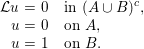 $$\begin{eqnarray}\begin{array}{@{}rcll@{}}{\mathcal{L}}u\ & =\ & 0\quad & \text{in }(A\cup B)^{c},\\ u\ & =\ & 0\quad & \text{on }A,\\ u\ & =\ & 1\quad & \text{on }B.\end{array}\end{eqnarray}$$
This function plays an important role in importance sampling (as
explained here) but also in optimal splitting techniques (Vanden-Eijnden,
Venturoli, Ciccotti and Elber Reference Vanden-Eijnden, Venturoli, Ciccotti and Elber2008,
Guyader Reference Guyader2015). It is also very useful for
theoretical purposes, to compute transition rates from  $A$ to
 $B$ (E and Vanden-Eijnden Reference E and Vanden-Eijnden2004, Hummer Reference Hummer2004, Lu and Nolen
Reference Lu and Nolen2015).
Second, the function  $u$ solution to (6.14), used here to build an optimal importance sampling scheme, can also
be used to build an optimal control variate (see Section 3.4.2 for an introduction to variance
reduction by control variates). Indeed, by Itô calculus, it is easy to
check that if
 $u$ satisfies (6.14) and
 $(q_{t})_{t\geqslant 0}$ follows overdamped Langevin dynamics (1.8), then
 $$\begin{eqnarray}\displaystyle u(q_{t})\exp \biggl(\int _{0}^{t}f(q_{s})\,\text{d}s\biggr) & = & \displaystyle u(q_{0})+\int _{0}^{t}({\mathcal{L}}u+fu)(q_{s})\exp \biggl(\int _{0}^{s}f(q_{r})\,\text{d}r\biggr)\,\text{d}s\nonumber\\ \displaystyle & & \displaystyle \quad +\sqrt{2{\it\beta}^{-1}}\int _{0}^{t}\exp \biggl(\int _{0}^{s}f(q_{r})\,\text{d}r\biggr){\rm\nabla}u(q_{s})\cdot \,\text{d}W_{s}\nonumber\end{eqnarray}$$
so that, by choosing  $t={\it\tau}$ (see (6.17), with
 $x_{0}=q_{0}$),
 $$\begin{eqnarray}\exp \biggl(g(q_{{\it\tau}})+\int _{0}^{{\it\tau}}f(q_{s})\,\text{d}s\biggr)=I+\sqrt{2{\it\beta}^{-1}}\int _{0}^{{\it\tau}}\exp \biggl(\int _{0}^{s}f(q_{r})\,\text{d}r\biggr){\rm\nabla}u(q_{s})\cdot \,\text{d}W_{s}.\end{eqnarray}$$
On the left-hand side, one recognizes the unbiased estimator  $\hat{I}$ (see (6.8)) of
 $I$, and from this equality, one can see that
 $$\begin{eqnarray}\hat{Z}=\sqrt{2{\it\beta}^{-1}}\int _{0}^{{\it\tau}}\exp \biggl(\int _{0}^{s}f(q_{r})\,\text{d}r\biggr){\rm\nabla}u(q_{s})\cdot \,\text{d}W_{s}\end{eqnarray}$$
is an optimal control variate for  $\hat{I}$, since
 $\mathbb{E}(\hat{Z})=0$ and
 $$\begin{eqnarray}\text{Var}(\hat{I} -\hat{Z})=0.\end{eqnarray}$$
This shows that a good approximation of the solution to (6.14) could also be used to build a good control variate.
6.3 The quasi-stationary distribution and the exit event from a metastable state
As mentioned in the introduction of Section 6, the difficulty when sampling paths of overdamped Langevin or Langevin
dynamics is that the system remains trapped for very long times in metastable states.
In this section we analyse the exit event from such a metastable state, denoted by  $S\subset {\mathcal{D}}$ in the following.
An interesting mathematical tool to study the exit event is the quasi-stationary
distribution (QSD). The reason why a partial differential equation is involved in
this problem is that the QSD attached to a state  $S$ is simply the first eigenvector of the Fokker–Planck
operator with homogeneous Dirichlet boundary conditions on
 $\partial S$.
6.3.1 The quasi-stationary distribution
Let us consider a fixed state  $S$ (i.e. an open boundedFootnote 19 and smooth subset of the configurational space
 ${\mathcal{D}}$) and let us focus for simplicity on overdamped Langevin dynamics
(1.8). Consider the first exit
time from
 $S$:
 $$\begin{eqnarray}{\it\tau}_{S}=\inf \{t\geqslant 0,\,q_{t}\not \in S\},\end{eqnarray}$$
where  $(q_{t})_{t\geqslant 0}$ follows overdamped Langevin dynamics (1.8).
Let us start with the definition of the QSD.
Definition 6.4. A probability measure  ${\it\nu}_{S}$ with support in
 $S$ is called a QSD for the Markov process
 $(q_{t})_{t\geqslant 0}$ if and only if
 $$\begin{eqnarray}{\it\nu}_{S}(A)=\frac{\int _{S}\mathbb{P}^{x}(q_{t}\in A,t<{\it\tau}_{S})\,{\it\nu}_{S}(\text{d}x)}{\int _{S}\mathbb{P}^{x}(t<{\it\tau}_{S})\,{\it\nu}_{S}(\text{d}x)},\quad \text{for all }t>0,~A\subset S.\end{eqnarray}$$
We recall that  $\mathbb{P}^{x}$ denotes the probability measure under which
 $q_{0}=x$. In other words,
 ${\it\nu}_{S}$ is a QSD if, when
 $q_{0}$ is distributed according to
 ${\it\nu}_{S}$, the law of
 $q_{t}$, conditional on
 $(q_{s})_{0\leqslant s\leqslant t}$ remaining in the state
 $S$, is still
 ${\it\nu}_{S}$, for all positive
 $t$.
The QSD satisfies three properties which will be crucial in the following. We refer for example to Le Bris, Lelièvre, Luskin and Perez (Reference Le Bris, Lelièvre, Luskin and Perez2012) for detailed proofs of these results and to Collet, Martínez and San Martín (Reference Collet, Martínez and San Martín2013) for more general results on QSDs.
Proposition 6.5. Let  $(q_{t})_{t\geqslant 0}$ follow the dynamics (1.8) with an initial condition
 $q_{0}$ distributed according to a distribution
 ${\it\nu}_{\text{init}}$ with support in
 $S$. Then there exists a probability distribution
 ${\it\nu}_{S}$ with support in
 $S$ such that, for any initial distribution
 ${\it\nu}_{\text{init}}$ with support in
 $S$,
 $$\begin{eqnarray}\lim _{t\rightarrow \infty }\text{Law}(q_{t}|{\it\tau}_{S}>t)={\it\nu}_{S}.\end{eqnarray}$$
The distribution  ${\it\nu}_{S}$ is the QSD associated with
 $S$.
A consequence of this proposition is the existence and uniqueness of the QSD. The
QSD is the long-time limit of the law of the (time marginal of the) process
conditioned to stay in the state  $S$: it can be seen as a ‘local ergodic
measure’ for the stochastic process in
 $S$. This proposition can be useful for properly defining a
metastable state. A metastable state is a state such that the typical exit time is
much larger than the local equilibration time, namely the time to observe the
convergence to the QSD in (6.26); see Section 6.4.1 for a precise discussion of this point.
Let us now give a second property of the QSD.
Proposition 6.6. Let  ${\mathcal{L}}=-{\rm\nabla}V\cdot {\rm\nabla}+{\it\beta}^{-1}{\rm\Delta}$ be the infinitesimal generator of
 $(q_{t})_{t\geqslant 0}$ (satisfying (1.8)). Let us consider the first eigenvalue and eigenfunction
associated with the adjoint operator
 ${\mathcal{L}}^{\dagger }=\text{div}({\rm\nabla}V+{\it\beta}^{-1}{\rm\nabla})$ with a homogeneous Dirichlet boundary condition:
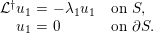 $$\begin{eqnarray}\begin{array}{@{}rcll@{}}{\mathcal{L}}^{\dagger }u_{1}\ & =\ & -{\it\lambda}_{1}u_{1}\quad & \text{on }S,\\ u_{1}\ & =\ & 0\quad & \text{on }\partial S.\end{array}\end{eqnarray}$$
Then, the QSD  ${\it\nu}_{S}$ associated with
 $S$ satisfies
 $$\begin{eqnarray}\text{d}{\it\nu}_{S}=\frac{u_{1}(x)\,\text{d}x}{\int _{S}u_{1}(x)\,\text{d}x},\end{eqnarray}$$
where  $\text{d}x$ denotes the Lebesgue measure on
 $S$.
The QSD thus has a density with respect to Lebesgue measure, which is simply the
ground state of the Fokker–Planck operator  ${\mathcal{L}}^{\dagger }$ associated with the dynamics with absorbing boundary conditions.
In (6.27), it can be shown that
 $u_{1}$ has a constant sign and hence can be chosen non-negative. In
addition,
 ${\it\lambda}_{1}>0$. Let us give the main arguments of the proof of this proposition
(see Le Bris et al. Reference Le Bris, Lelièvre, Luskin and Perez2012 for more details).
Proof. Let us first notice the equivalence between two properties:  $(-{\it\lambda}_{1},u_{1})$ is an eigenvalue–eigenfunction pair for
 ${\mathcal{L}}^{\dagger }$ (with zero Dirichlet boundary condition on
 $\partial S$) and
 $(-{\it\lambda}_{1},u_{1}\exp ({\it\beta}V))$ is an eigenvalue–eigenfunction pair for
 ${\mathcal{L}}$ (with zero Dirichlet boundary condition on
 $\partial S$). This is a simple consequence of the following identity:
for any
 $C^{\infty }$ test function
 ${\it\varphi}:{\mathcal{D}}\rightarrow \mathbb{R}$,
 $$\begin{eqnarray}{\mathcal{L}}^{\dagger }({\it\varphi}\exp (-{\it\beta}V))=({\mathcal{L}}{\it\varphi})\exp (-{\it\beta}V).\end{eqnarray}$$
Now, the operator  ${\mathcal{L}}$ with homogeneous Dirichlet boundary condition is symmetric
for the weighted
 $L^{2}({\it\nu})$ scalar product (where, we recall,
 ${\it\nu}(\text{d}q)=Z_{{\it\nu}}^{-1}\exp (-{\it\beta}V(q))\,\text{d}q$ is the canonical measure: see (1.5)). For any two
 $C^{\infty }$ test functions
 ${\it\varphi}$ and
 ${\it\psi}$ which vanish on
 $S^{c}$,
 $$\begin{eqnarray}\int _{S}{\it\varphi}({\mathcal{L}}{\it\psi})\,\text{d}{\it\nu}=\int _{S}{\it\psi}({\mathcal{L}}{\it\varphi})\,\text{d}{\it\nu}=-{\it\beta}^{-1}\int _{S}{\rm\nabla}{\it\varphi}\cdot {\rm\nabla}{\it\psi}\,\text{d}{\it\nu}.\end{eqnarray}$$
Since  $V$ is assumed to be
 $C^{\infty }$ and
 $S$ bounded, the inverse of the operator
 ${\mathcal{L}}$ from
 $L^{2}({\it\nu})$ to
 $L^{2}({\it\nu})$ is compact and symmetric. Thus
 ${\mathcal{L}}$ admits a discrete spectrum, and in particular a smallest
eigenvalue
 $-{\it\lambda}_{1}$ associated with an eigenvector
 ${\it\varphi}_{1}$. Using standard arguments, one can show that
 ${\it\varphi}_{1}>0$ and
 $-{\it\lambda}_{1}$ is a non-degenerate eigenvalue.
Let us now introduce the probability density  $u_{1}=Z_{S}^{-1}{\it\varphi}_{1}\exp (-{\it\beta}V)$ with
 $Z_{S}=\int _{S}{\it\varphi}_{1}\exp (-{\it\beta}V)$. As explained at the beginning of the proof,
 $({\it\lambda}_{1},u_{1})$ satisfies (6.27). Let us prove that
 $u_{1}(x)\,\text{d}x$ is a QSD, by checking (6.25). Fix a subset
 $A$ of
 $S$ and introduce
 $v(t,x)=\mathbb{P}^{x}(q_{t}\in A,t<{\it\tau}_{S})$ as well as
 $\overline{v}(t,x)=\mathbb{P}^{x}(t<{\it\tau}_{S})$. From Proposition 6.1, the function
 $v$ satisfies
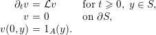 $$\begin{eqnarray}\begin{array}{@{}rcll@{}}\partial _{t}v\ & =\ & {\mathcal{L}}v\quad & \text{for }t\geqslant 0,\;y\in S,\\ v\ & =\ & 0\quad & \text{on }\partial S,\\ v(0,y)\ & =\ & 1_{A}(y).\quad & \end{array}\end{eqnarray}$$
Likewise, the function  $\overline{v}$ satisfies the same equation, with initial condition
 $\overline{v}(0,y)=1$. Therefore,
 $$\begin{eqnarray}\displaystyle & & \displaystyle \frac{\text{d}}{\text{d}t}\biggl(\int _{S}\mathbb{P}^{x}(q_{t}\in A,t<{\it\tau}_{S})u_{1}(x)\,\text{d}x\biggr)\nonumber\\ \displaystyle & & \displaystyle \qquad =Z_{S}^{-1}\frac{\text{d}}{\text{d}t}\biggl(\int _{S}v(t,\cdot ){\it\varphi}_{1}\exp (-{\it\beta}V)\biggr)\nonumber\\ \displaystyle & & \displaystyle \qquad =Z_{S}^{-1}\int _{S}({\mathcal{L}}v){\it\varphi}_{1}\exp (-{\it\beta}V)\nonumber\\ \displaystyle & & \displaystyle \qquad =Z_{S}^{-1}\int _{S}v({\mathcal{L}}{\it\varphi}_{1})\exp (-{\it\beta}V)\nonumber\\ \displaystyle & & \displaystyle \qquad =-{\it\lambda}_{1}Z_{S}^{-1}\int _{S}v{\it\varphi}_{1}\exp (-{\it\beta}V)\nonumber\\ \displaystyle & & \displaystyle \qquad =-{\it\lambda}_{1}\int _{S}\mathbb{P}^{x}(q_{t}\in A,t<{\it\tau}_{S})u_{1}(x)\,\text{d}x,\nonumber\end{eqnarray}$$
which yields
 $$\begin{eqnarray}\int _{S}\mathbb{P}^{x}(q_{t}\in A,t<{\it\tau}_{S})u_{1}(x)\,\text{d}x=\biggl(\int _{A}u_{1}(x)\,\text{d}x\biggr)\exp (-{\it\lambda}_{1}t).\end{eqnarray}$$
Likewise, considering  $\overline{v}$, it is easy to check that (taking
 $A=S$ in (6.28))
 $$\begin{eqnarray}\int _{S}\mathbb{P}^{x}(t<{\it\tau}_{S})u_{1}(x)\,\text{d}x=\exp (-{\it\lambda}_{1}t).\end{eqnarray}$$
This concludes the proof in view of (6.25).
Finally, the third property of the QSD concerns the exit event, when  $q_{0}$ is distributed according to
 ${\it\nu}_{S}$.
Proposition 6.7. Let us assume that  $q_{0}$ is distributed according to the QSD
 ${\it\nu}_{S}$ in
 $S$. Then the law of the pair
 $({\it\tau}_{S},q_{{\it\tau}_{S}})$ (i.e. the first exit time and
the first exit point) is fully characterized by the following properties.
∙
${\it\tau}_{S}$ is exponentially distributed with parameter ${\it\lambda}_{1}$ (defined in (6.27)).∙
${\it\tau}_{S}$ is independent of $q_{{\it\tau}_{S}}$.∙ The law of
$q_{{\it\tau}_{S}}$ is given as follows: for any bounded measurable
function ${\it\varphi}:\partial S\rightarrow \mathbb{R}$, (6.30)where$$\begin{eqnarray}\mathbb{E}^{{\it\nu}_{S}}({\it\varphi}(q_{{\it\tau}_{S}}))=-\frac{\int _{\partial S}{\it\varphi}\,\partial _{n}u_{1}\,\text{d}{\it\sigma}}{{\it\beta}{\it\lambda}_{1}\int _{S}u_{1}(x)\,\text{d}x},\end{eqnarray}$$${\it\sigma}$ denotes the Lebesgue measure on $\partial S$ induced by the Lebesgue measure on ${\mathcal{D}}$ and the Euclidean scalar product, and $\partial _{n}u_{1}={\rm\nabla}u_{1}\cdot n$ denotes the outward normal derivative of $u_{1}$ (defined in (6.27)) on $\partial S$.





In (6.30), the superscript  ${\it\nu}_{S}$ indicates that the initial condition
 $q_{0}$ is assumed to be distributed according to
 ${\it\nu}_{S}$. Let us give a brief proof of this important result (see again
Le Bris et al. Reference Le Bris, Lelièvre, Luskin and Perez2012 for more details).
Proof. The fact that  ${\it\tau}_{S}$ is exponentially distributed with parameter
 ${\it\lambda}_{1}$ is a direct consequence of (6.29). To prove the two remaining items, let us
consider the solution
 $v$ to the following PDE:
 $$\begin{eqnarray}\begin{array}{@{}rcll@{}}\partial _{t}v\ & =\ & {\mathcal{L}}v\quad & \text{for }t\geqslant 0,\;x\in S,\\ v\ & =\ & {\it\varphi}\quad & \text{on }\partial S,\\ v(0,x)\ & =\ & 0\quad & \text{for }x\in S.\end{array}\end{eqnarray}$$
From Proposition 6.1, we have the probabilistic representation formula
 $$\begin{eqnarray}v(t,x)=\mathbb{E}^{x}(1_{{\it\tau}_{S}<t}\,{\it\varphi}(q_{{\it\tau}_{S}})).\end{eqnarray}$$
Let us introduce
 $$\begin{eqnarray}f(t)=\mathbb{E}^{{\it\nu}_{S}}(1_{{\it\tau}_{S}<t}\,{\it\varphi}(q_{{\it\tau}_{S}}))=\int _{S}\mathbb{E}^{x}(1_{{\it\tau}_{S}<t}\,{\it\varphi}(q_{{\it\tau}_{S}})){\it\nu}_{S}(\text{d}x)=Z_{S}^{-1}\int _{S}v(t,\cdot )u_{1},\end{eqnarray}$$
where  $Z_{S}=\int _{S}u_{1}$. Using integration by parts and the fact that
 $u_{1}=0$ on
 $\partial S$, we obtain
 $$\begin{eqnarray}\displaystyle f^{\prime } & = & \displaystyle Z_{S}^{-1}\int _{S}\partial _{t}v\,u_{1}\nonumber\\ \displaystyle & = & \displaystyle Z_{S}^{-1}\int _{S}({\mathcal{L}}v)u_{1}=Z_{S}^{-1}\int _{S}(-{\rm\nabla}V\cdot {\rm\nabla}v+{\it\beta}^{-1}{\rm\Delta}v)u_{1}\nonumber\\ \displaystyle & = & \displaystyle Z_{S}^{-1}\int _{S}v(\text{div}(u_{1}{\rm\nabla}V)+{\it\beta}^{-1}{\rm\Delta}u_{1})-Z_{S}^{-1}{\it\beta}^{-1}\int _{\partial S}v\partial _{n}u_{1}\,\text{d}{\it\sigma}\nonumber\\ \displaystyle & = & \displaystyle -{\it\lambda}_{1}f-Z_{S}^{-1}{\it\beta}^{-1}\int _{\partial S}{\it\varphi}\partial _{n}u_{1}\,\text{d}{\it\sigma}.\nonumber\end{eqnarray}$$
By solving this ordinary differential equation in  $f$, we thus get
 $$\begin{eqnarray}f(t)=\mathbb{E}^{{\it\nu}_{S}}(1_{{\it\tau}_{S}<t}\,{\it\varphi}(q_{{\it\tau}_{S}}))=(1-\exp (-{\it\lambda}_{1}t))\int _{\partial S}{\it\varphi}\,\text{d}{\it\rho},\end{eqnarray}$$
where  ${\it\rho}$ denotes the probability measure
 $$\begin{eqnarray}\text{d}{\it\rho}=-\frac{{\it\beta}^{-1}}{{\it\lambda}_{1}Z_{S}}\partial _{n}u_{1}\,\text{d}{\it\sigma}.\end{eqnarray}$$
Note that  $\partial _{n}u_{1}\leqslant 0$ and
 $Z_{S}\geqslant 0$ when
 $u_{1}$ is chosen positive in
 $S$, hence
 ${\it\rho}$ indeed has a non-negative density with respect to
 ${\it\sigma}$. Since
 $1-\exp (-{\it\lambda}_{1}t)=\mathbb{P}^{{\it\nu}}({\it\tau}_{S}<t)$, equation (6.31) shows that, if
 $q_{0}\sim {\it\nu}_{S}$, the random variables
 ${\it\tau}_{S}$ and
 $q_{{\it\tau}_{S}}$ are independent, and
 $q_{{\it\tau}_{S}}$ is distributed according to
 ${\it\rho}$. This concludes the proof of Proposition 6.7.
Remark 6.8. The existence of the QSD and the convergence of the conditioned process towards the QSD for the Langevin process (1.9) require extra work compared to the overdamped Langevin process (1.8). For results in that direction, we refer to the recent paper by Nier (Reference Nier2014).
6.3.2 Exit event and the state-to-state dynamics
Proposition 6.7 explains
the role of the QSD in relating the continuous-in-time process  $(q_{t})_{t\geqslant 0}$ to a jump process between metastable states.
Indeed, if the process remains for a long time in  $S$, then, according to Proposition 6.5, it is approximately distributed
according to the QSD. Therefore, to study the exit from
 $S$, it is relevant to consider a process starting from
 ${\it\nu}_{S}$ and to look at the pair
 $({\it\tau}_{S},q_{{\it\tau}_{S}})$ which fully characterizes the exit event from
 $S$. Proposition 6.7 shows that the exit event from the state
 $S$ is Markovian. It can be rewritten as one step of a Markov jump
process, thanks to two important properties:
 ${\it\tau}_{S}$ is exponentially distributed and independent of
 $q_{{\it\tau}_{S}}$. This is reminiscent of what is assumed to build kinetic Monte
Carlo (Voter Reference Voter, Sickafus, Kotomin and Uberuaga2007) or Markov state models
(Sarich and Schütte Reference Sarich and Schütte2013,
Bowman et al. Reference Bowman, Pande and Noé2014).
Let us make this more precise. The aim is to build from the continuous state-space
dynamics  $(q_{t})_{t\geqslant 0}$ a discrete state-space dynamics, which jumps from state to
state. Let us assume that we are given a mapping
 $$\begin{eqnarray}{\mathcal{S}}:{\mathcal{D}}\rightarrow \mathbb{N},\end{eqnarray}$$
which to any given  $x\in {\mathcal{D}}$ associates
 ${\mathcal{S}}(x)$, the label of the state in which
 $x$ lies. The mapping
 ${\mathcal{S}}$ thus defines a partition of the state space. In the simple
two-dimensional case of Figure 1.1, for example, one could use just two states:
 ${\mathcal{S}}(x,y)$ is
 $0$ if
 $x<0$ and
 $1$ if
 $x>0$. The state-to-state dynamics is then simply the dynamics
 $$\begin{eqnarray}({\mathcal{S}}(q_{t}))_{t\geqslant 0},\end{eqnarray}$$
where  $(q_{t})_{t\geqslant 0}$ is obtained by the Langevin (1.9) or overdamped Langevin (1.8) dynamics. Of course this is not a Markovian dynamics. If
 ${\mathcal{S}}$ is well chosen, however, it is close to a Markovian dynamics. In
the next section we will come back to one way to correct for non-Markovian
effects. We concentrate here on the parametrization of the Markov dynamics
associated with the partition and the original dynamics. Let us assume that the
process
 $(q_{t})_{t\geqslant 0}$ remains in one of the components of the partition for a
sufficiently long time, so that the limit in (6.26) is reached (see Proposition 6.9 for an estimate of this
convergence time). Let
 $S$ denote this state:
 $S={\mathcal{S}}^{-1}(\{n\})$ for some
 $n\in \mathbb{N}$.
The state  $S$ with the partition of the boundary
 $\partial S$ into four subsets
 $(\partial S_{i})_{i=1,\ldots ,4}$. The dashed line represents the trajectory of a
dynamics entering
 $S$.
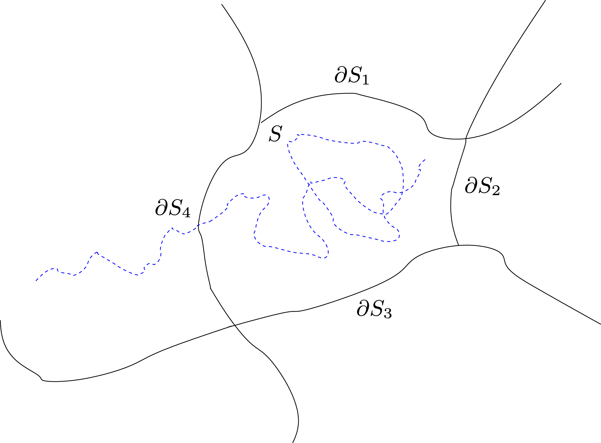
Let us now assume that the state  $S$ is surrounded by
 $I$ neighbouring states. The boundary
 $\partial S$ is then divided into
 $I$ disjoint subsets
 $(\partial S_{i})_{i=1,\ldots ,I}$, each of them associated with an exit towards one of the
neighbouring states (see Figure 6.1 for a situation where
 $I=4$). The exit event from
 $S$ is characterized by the pair
 $({\it\tau}_{S},{\mathcal{I}})$, where
 ${\mathcal{I}}$ is a random variable which gives the next visited state:
 $$\begin{eqnarray}\text{for }i=1,\ldots ,I,\quad \{{\mathcal{I}}=i\}=\{q_{{\it\tau}_{S}}\in \partial S_{i}\}.\end{eqnarray}$$
Notice that  ${\it\tau}_{S}$ and
 ${\mathcal{I}}$ are independent random variables. The kinetic Monte Carlo model
is then parametrized as follows. Introduce
 $$\begin{eqnarray}p(i)=\mathbb{P}(q_{{\it\tau}_{S}}\in \partial S_{i})=-\frac{\int _{\partial S_{i}}\partial _{n}u_{1}\,\text{d}{\it\sigma}}{{\it\beta}{\it\lambda}_{1}\int _{S}u_{1}\,\text{d}x},\quad \text{for }i=1,\ldots ,I.\end{eqnarray}$$
For each exit region  $\partial S_{i}$ there is a corresponding rate
 $k(i)={\it\lambda}_{1}p(i)$. Now, if
 $(T_{i})_{i=1,\ldots ,I}$ are independent random variables, where
 $T_{i}$ is exponentially distributed with parameter
 $k(i)$, one can check that
 $$\begin{eqnarray}({\it\tau}_{S},{\mathcal{I}})\stackrel{{\mathcal{L}}}{=}\biggl(\min _{i\in \{1,\ldots ,I\}}(T_{i}),\text{arg\,min}_{i\in \{1,\ldots ,I\}}(T_{i})\biggr),\end{eqnarray}$$
where  $\stackrel{{\mathcal{L}}}{=}$ denotes equality in law. A natural way to parametrize a kinetic
Monte Carlo model associated with the partition
 $({\mathcal{S}}^{-1}(\{n\}))_{n\in \mathbb{N}}$ is thus to consider the stochastic process starting from the QSD
associated with each state, and to use the random variables
 $({\it\tau}_{S},q_{{\it\tau}_{S}})$ to parametrize the jump process. In practice, computing the
rates
 $k(i)$ associated with
 $S$ may be complicated. Most often, rates are evaluated using an
approximation (Voter Reference Voter, Sickafus, Kotomin and Uberuaga2007, Berglund Reference Berglund2013): for instance the harmonic
transition state theory, the Arrhenius law, or the Eyring–Kramers law
(see formula (6.39) below).
We have discussed one natural way to relate a continuous state-space dynamics to a
discrete state-space dynamics: introduce a partition of the state space and
consider the position of the process within this partition. Another natural idea
is to introduce an ensemble of disjoint subsets  $(M_{i})_{i\geqslant 1}$ and to project the dynamics
 $(q_{t})_{t\geqslant 0}$ onto a discrete state-space dynamics by considering the last
visited milestone (Buchete and Hummer Reference Buchete and Hummer2008,
Schütte, Noé, Lu, Sarich and Vanden-Eijnden Reference Schütte, Noé, Lu, Sarich and Vanden-Eijnden2011). Notice that these subsets do not
create a partition of the state space. They are sometimes called milestones
(Faradjian and Elber Reference Faradjian and Elber2004), target sets or
core sets (Schütte et al. Reference Schütte, Noé, Lu, Sarich and Vanden-Eijnden2011) in the literature. The natural
parametrization of the underlying jump process is then to consider, starting from
a milestone (say
 $M_{1}$), the time to reach any of the other milestones
 $(M_{j})_{j\neq 1}$ and the index of the next visited milestone. This requires us to
study the reactive paths among the milestones, for which many techniques have been
proposed (Dellago and Bolhuis Reference Dellago and Bolhuis2009): for
example, transition interface sampling (van Erp, Moroni and Bolhuis Reference van Erp, Moroni and Bolhuis2003, van Erp and Bolhuis Reference van Erp and Bolhuis2005), forward flux sampling (Allen, Warren
and ten Wolde Reference Allen, Warren and ten Wolde2005, Allen, Valeriani and ten
Wolde Reference Allen, Valeriani and ten Wolde2009), the string method (E and
Vanden-Eijnden Reference E and Vanden-Eijnden2004, E, Ren and
Vanden-Eijnden Reference E, Ren and Vanden-Eijnden2002, Reference E, Ren and Vanden-Eijnden2005), and adaptive multilevel splitting techniques
(Cérou and Guyader Reference Cérou and Guyader2007,
Cérou, Guyader, Lelièvre and Pommier Reference Cérou, Guyader, Lelièvre and Pommier2011). Reactive paths are the pieces of a trajectory at
equilibrium between metastable states: see Hummer (Reference Hummer2004), E and Vanden-Eijnden (Reference E and Vanden-Eijnden2004) and Lu and Nolen (Reference Lu and Nolen2015). Let us finally discuss the error introduced by this
approach, namely the Markovianity of the projected dynamics. On the one hand, in
the limit of very small milestones,Footnote 20 the sequence of visited states
(i.e. the skeleton of the projected process) is
naturally Markovian (even though the transition time is not necessarily
exponential), but the description of the underlying continuous state-space
dynamics is very poor (since the information of the last visited milestone is not
very informative about the actual state of the system). On the other hand, taking
larger milestones, the projected process is close to a Markov process under some
metastability assumptions with respect to these milestones. We refer to Sarich,
Noé and Schütte (Reference Sarich, Noé and Schütte2010), Sarich and Schütte (Reference Sarich and Schütte2013) and Bovier and den Hollander (Reference Bovier and den Hollander2015) for a mathematical analysis.
6.4 Accelerated dynamics
The idea of the numerical methods presented in this section is to take advantage of metastability in order to simulate paths over very long time scales more efficiently. In the spirit of a predictor–corrector method, the principle is indeed to use the underlying Markov jump process to more efficiently simulate the original dynamics, or more precisely the state-to-state dynamics which encodes the ambient metastable state at a given time (see equation (6.33)). These techniques, called accelerated dynamics, were introduced by Voter and his co-workers in the late 1990s.
Using the notation of the previous section, let us consider a function  ${\mathcal{S}}:{\mathcal{D}}\rightarrow \mathbb{N}$ which defines a partition of the state space. The aim of
accelerated dynamics techniques is to efficiently generate paths of the dynamics
 $({\mathcal{S}}(q_{t}))_{t\geqslant 0}$. As explained above, this is not a Markovian dynamics but, if
 ${\mathcal{S}}$ is well chosen, it is close to a Markovian dynamics. The main idea
of accelerated dynamics is to take advantage of this fact, by checking the
Markovianity on-the-fly (see Section 6.4.1 below). However – and this is very important –
we show below that for any mapping
 ${\mathcal{S}}$, the accelerated dynamics are consistent, in the sense that they
simulate the state-to-state dynamics (6.33) up to an error term which goes to zero when certain numerical
parameters go to zero. Somehow, the mapping
 ${\mathcal{S}}$ is very similar to the reaction coordinate
 ${\it\xi}$ introduced in Section 4.1, except that it takes values in a discrete state space (which can be
chosen to be
 $\mathbb{N}$ without loss of generality: see (6.32)). For further comments on the
practical way to choose
 ${\mathcal{S}}$, we refer to Remark 6.11 below.
Given the mapping  ${\mathcal{S}}$, the principal idea of accelerated dynamics algorithms is as
follows: if the stochastic process remains trapped for a very long time in a given
state
 $S={\mathcal{S}}^{-1}(\{n\})$ (for some
 $n$), then it has ‘lost its memory’, and there is
a way to generate the exit event from this state much more efficiently than by
running the original dynamics until the exit time. This is formalized mathematically
below. These algorithms thus efficiently simulate the exit event from
 $S$, which means that they efficiently sample the pair of random
variables
 $({\it\tau}_{S},q_{{\it\tau}_{S}})$. Thanks to these techniques, one efficiently samples the
state-to-state dynamics
 $({\mathcal{S}}(q_{t}))_{t\geqslant 0}$. Let us emphasize that the aim is to get the correct law on the
paths (in order to be able to compute dynamical quantities, such as the typical time
to go from one state to another). This is much more demanding than, for example,
simply computing the relative likelihood of the states
 $({\mathcal{S}}^{-1}(\{n\}))_{n\in \mathbb{N}}$ (which is equivalent to computing the free energy associated with
 ${\mathcal{S}}$: see Section 4.1).
Three algorithms have been proposed by Voter and co-workers. Before going into the details, let us briefly describe the ideas behind these three algorithms.
In the Parallel Replica method (Voter Reference Voter1998), the principle is to simulate in parallel many trajectories following the original dynamics (1.9) or (1.8), to consider the first exit event among the replicas, and to generate from this first exit event a consistent exit time and exit point. The gain is thus obtained in terms of wall clock time. This algorithm can be seen as a way to parallelize a computation in time, which is not an easy problem in general due to the sequential nature of the time evolution.
In the Hyperdynamics method (Voter Reference Voter1997), the
idea is to modify the potential  $V$ within the state
 $S$ in order to accelerate the exit from the state for the original
dynamics (1.9) or (1.8). Again, using an appropriate time
rescaling, it is possible to generate from the observed exit event on the biased
potential an exit event which is consistent with what would have been observed on the
original unbiased potential
 $V$.
The Temperature Accelerated Dynamics (TAD) method (Sorensen and Voter Reference Sorensen and Voter2000) considers the original dynamics (1.9) or (1.8) at a higher temperature than the original one. The idea is then that, under appropriate assumptions, there is a way to infer from the exit events observed at high temperature the exit event which would have been observed at the original lower temperature.
This section is organized as follows. In Section 6.4.1 we present the decorrelation step: this is used in practice to assess whether the process has remained sufficiently long in a state that one can assume it is distributed according to the QSD. In Sections 6.4.2–6.4.4 we successively introduce the three algorithms: Parallel Replica, Hyperdynamics, and Temperature Accelerated Dynamics. Section 6.4.5 is devoted to some concluding remarks.
6.4.1 The decorrelation step
The accelerated dynamics algorithms are based on the assumption that the process
remains sufficiently long in the state  $S$ that it can be assumed to be distributed according to the QSD
 ${\it\nu}_{S}$.
A natural preliminary question is therefore how to assess in practice that the
limit has been reached in (6.26). This is done in the so-called decorrelation step, which consists in
waiting for a given time  $t_{\text{corr}}$ (a so-called decorrelation time) before assuming that the local
equilibrium
 ${\it\nu}_{S}$ has been reached. This correlation time can be state-dependent,
and is typically assumed to be known a priori. However, let us mention
the recent work of Binder, Simpson and Lelièvre (Reference Binder, Simpson and Lelièvre2015), where a numerical method is proposed in order to
approximate the time to reach the QSD using a Fleming–Viot particle
process together with convergence diagnostics.
From a mathematical viewpoint,  $t_{\text{corr}}$ should be chosen sufficiently large that the distance between
the law of
 $q_{t_{\text{corr}}}$ conditioned to
 ${\it\tau}_{S}\geqslant t_{\text{corr}}$ and the QSD
 ${\it\nu}_{S}$ is small. Le Bris et al. (Reference Le Bris, Lelièvre, Luskin and Perez2012) prove the following result.
Proposition 6.9. Let  $(q_{t})_{t\geqslant 0}$ satisfy (1.8) with
 $q_{0}\in S$. Introduce the first two eigenvalues
 $-{\it\lambda}_{2}<-{\it\lambda}_{1}<0$ of the operator
 ${\mathcal{L}}^{\dagger }$ on
 $S$ with homogeneous Dirichlet boundary conditions on
 $\partial S$ (see Proposition 6.6 for the definition of
 ${\mathcal{L}}^{\dagger }$). Then there exists a constant
 $C>0$ (which depends on the law of
 $q_{0}$), such that, for all
 $t\geqslant C/({\it\lambda}_{2}-{\it\lambda}_{1})$,
 $$\begin{eqnarray}\sup _{f,\,\Vert f\Vert _{L^{\infty }}\leqslant 1}|\mathbb{E}(f({\it\tau}_{S}-t,q_{{\it\tau}_{S}})|{\it\tau}_{S}\geqslant t)-\mathbb{E}^{{\it\nu}_{S}}(f({\it\tau}_{S},q_{{\it\tau}_{S}}))|\leqslant C\exp (-({\it\lambda}_{2}-{\it\lambda}_{1})t).\end{eqnarray}$$
The supremum is taken over all bounded functions  $f:\mathbb{R}_{+}\times \partial S\rightarrow \mathbb{R}$, with
 $L^{\infty }$-norm smaller than one.
In other words, the total variation norm (2.26) between the law of  $({\it\tau}_{S}-t,q_{{\it\tau}_{S}})$ conditioned to
 ${\it\tau}_{S}\geqslant t$ (for any initial condition
 $q_{0}\in S$), and the law of
 $({\it\tau}_{S},q_{{\it\tau}_{S}})$ when
 $q_{0}$ is distributed according to
 ${\it\nu}_{S}$, decreases exponentially fast with rate
 ${\it\lambda}_{2}-{\it\lambda}_{1}$. This means that
 $t_{\text{corr}}$ should be chosen of order
 $1/({\it\lambda}_{2}-{\it\lambda}_{1})$. Of course, this is not a very practical result since computing
these eigenvalues is in general impossible. From a theoretical viewpoint, this
result tells us that the local equilibration time is of order
 $1/({\it\lambda}_{2}-{\it\lambda}_{1})$, so the state
 $S$ is metastable if this time is much smaller than the exit time
(which is typically of order
 $1/{\it\lambda}_{1}$: see Proposition 6.6).
From now on, we assume that the decorrelation step has been successful (the
process remained in  $S$ for a time
 $t_{\text{corr}}$), and we look for efficient techniques to generate the exit
event (i.e. a sample of the random variables
 $({\it\tau}_{S},q_{{\it\tau}_{S}})$) starting from the QSD. Let us describe in succession the three
algorithms proposed by Voter and his co-workers.
6.4.2 Parallel Replica
Consider an initial condition  $q_{0}\in S$ such that
 $q_{0}$ is distributed according to the QSD in
 $S$. Assume that we are given a computer with many CPUs in parallel.
The idea of the Parallel Replica method is to distribute
 $N$ independent initial conditions
 $(q_{0}^{i})_{1\leqslant i\leqslant N}$ in
 $S$ according to the QSD
 ${\it\nu}_{S}$, to let them evolve according to (1.8) driven by independent Brownian motions (so that the
replicas remain independent), and then to consider the first exit event among the
replicas:
 $$\begin{eqnarray}I_{0}=\text{arg\,min}_{i\in \{1,\ldots ,N\}}{\it\tau}_{S}^{i}\quad \text{where }{\it\tau}_{S}^{i}=\inf \{t\geqslant 0~:~q_{t}^{i}\not \in S\}.\end{eqnarray}$$
The integer  $I_{0}\in \{1,\ldots ,N\}$ is the index of the first replica to leave
 $S$, and
 $\min ({\it\tau}_{S}^{1},\ldots ,{\it\tau}_{S}^{N})={\it\tau}_{S}^{I_{0}}$. The effective exit time is set as
 $N$ times the first exit time, and the effective exit point is
simply the exit point for the first exit event.
Parallel Replica. Many exit events are simulated in
parallel, all starting from the QSD in  $S$. The dashed line trajectory represents the reference
walker, which stays sufficiently long within
 $S$ that we can assume the end point (circle) is
distributed according to the QSD. The other dots (squares) represent
i.i.d. initial conditions distributed according to the QSD.
The solid line trajectories are simulated in parallel.
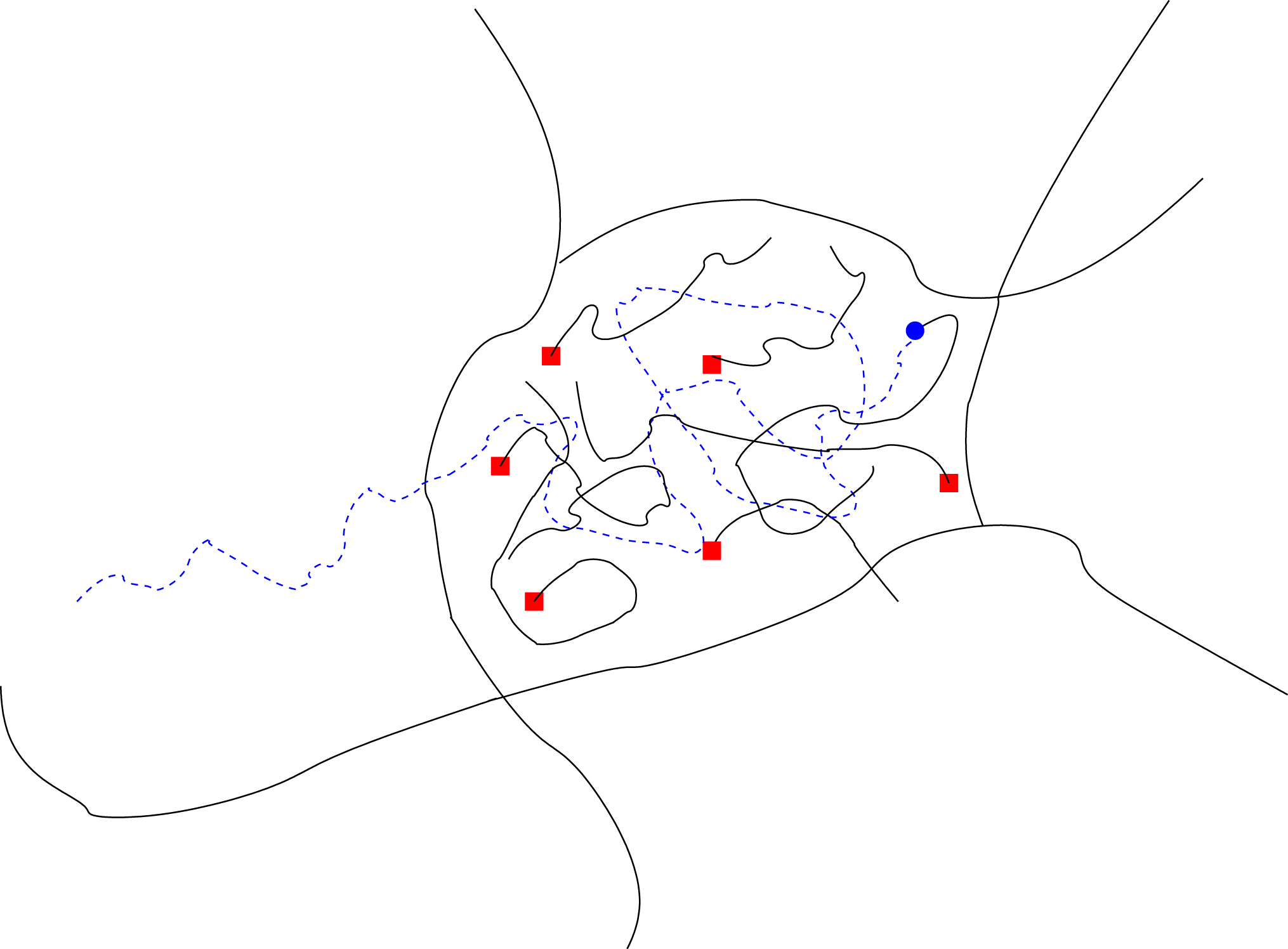
The consistency of the method is a corollary of Proposition 6.7. Indeed, using the fact that, starting from the QSD, the exit time is exponentially distributed and independent of the exit point, we easily obtain that
 $$\begin{eqnarray}N{\it\tau}_{S}^{I_{0}}=N\min ({\it\tau}_{S}^{1},\ldots ,{\it\tau}_{S}^{N})\stackrel{{\mathcal{L}}}{=}{\it\tau}_{S}^{1},\end{eqnarray}$$
which means that the effective exit time has the correct law, and
 $$\begin{eqnarray}X_{{\it\tau}_{S}^{I_{0}}}^{I_{0}}\stackrel{{\mathcal{L}}}{=}X_{{\it\tau}_{S}^{1}}^{1},\end{eqnarray}$$
which means that the first exit point of the replica  $I_{0}$ (the first one to exit among
 $N$) has the same law as the first exit point of any of them.
Moreover
 $$\begin{eqnarray}N{\it\tau}_{S}^{I_{0}}=N\min ({\it\tau}_{S}^{1},\ldots ,{\it\tau}_{S}^{N})\quad \text{and}\quad X_{{\it\tau}_{S}^{I_{0}}}^{I_{0}}\end{eqnarray}$$
are independent, so we have proved the following lemma.
Lemma 6.10. Let  $I_{0}$ be the index of the first replica exiting
 $S$, defined by (6.34). Then we have the equality in law
 $$\begin{eqnarray}(N{\it\tau}_{S}^{I_{0}},X_{{\it\tau}_{S}^{I_{0}}}^{I_{0}})\stackrel{{\mathcal{L}}}{=}({\it\tau}_{S}^{1},X_{{\it\tau}_{S}^{1}}^{1}).\end{eqnarray}$$
This lemma shows that Parallel Replica is exact: the law of the effective exit time and exit point is exactly the law of the exit time and exit point which would have been observed for only one replica.
Let us make a few remarks on this algorithm. First, the full algorithm actually iterates the following three steps; see Figure 6.2 for a schematic illustration of the method.
∙ The decorrelation step (see Section 6.4.1), where a reference walker is run following the dynamics (1.8) until it remains trapped for such a long time in one of the sets
${\mathcal{S}}^{-1}(\{n\})$ that it can be assumed to be distributed according to
the QSD ${\it\nu}_{S}$ associated with this set. During this step, the
algorithm thus simply integrates the original dynamics. No error is
introduced and there is no computational gain.∙ The dephasing step, which is a preparation step during which
$N$ independent initial conditions distributed according to ${\it\nu}_{S}$ are sampled, each one on a different CPU. This is done
in parallel. During this step the simulation clock is stopped. This step
is thus purely overhead. It requires appropriate algorithms to sample the
QSD such as the rejection algorithm or Fleming–Viot particle
systems (see Le Bris et al. Reference Le Bris, Lelièvre, Luskin and Perez2012). For example, the rejection
algorithm consists in running independent walkers following the dynamics
(1.8) (starting from a
point within $S$) and to consider the final point of the trajectory
conditional on the walker remaining in the state, for a sufficiently long
trajectory (typically for the time $t_{\text{corr}}$ introduced in the previous paragraph).∙ The parallel step, just described above, which consists in running the
$N$ replicas independently in parallel, and waiting for the
first exit event among the $N$ replicas. The simulation clock is then updated by
adding the effective exit time $N{\it\tau}_{S}^{I_{0}}$. The exit point $X_{{\it\tau}_{S}^{I_{0}}}^{I_{0}}$ is used as the initial condition of the reference
walker for the next decorrelation step. The computational gain of the
whole algorithm comes from this step, which divides the wall clock time
to sample the exit event by the number of replicas $N$.


In practice, if the rejection algorithm is used in the dephasing step, one does
not actually need to wait for the  $N$ replicas to be dephased to proceed to the parallel
step: see Voter (Reference Voter1998), Le Bris
et al. (Reference Le Bris, Lelièvre, Luskin and Perez2012) and Binder et al. (Reference Binder, Simpson and Lelièvre2015).
The Parallel Replica algorithm is very versatile; see Aristoff,
Lelièvre and Simpson (Reference Aristoff, Lelièvre and Simpson2014) for
an extension to Markov chains. In particular, it applies to both energetic and
entropic barriers. The only errors introduced in the algorithm are related to the
rate of convergence of the law of the conditioned process to the QSD. For an
analysis of the errors introduced by the algorithm and a discussion of the
parallel efficiency, we refer to Le Bris et al. (Reference Le Bris, Lelièvre, Luskin and Perez2012) and Binder
et al. (Reference Binder, Simpson and Lelièvre2015).
The algorithm is more efficient when the convergence time to the QSD is small
compared to the exit time (i.e., the states are metastable): in
this case, the speed-up in terms of wall clock time is linear as a function of  $N$.
Remark 6.11 (on the mapping ${\mathcal{S}}$).

Let us comment on the mapping  ${\mathcal{S}}$ which defines the states. These comments are actually also
relevant to the two other algorithms (Hyperdynamics and TAD). First, from a
practical viewpoint, it is important to notice that the numbering of the
states need not be defined a priori: the states are numbered as
the simulation proceeds, when they are successively discovered by the
stochastic process.
Now, an important question is how to choose the partition  $({\mathcal{S}}^{-1}(\{n\}))_{n\in \mathbb{N}}$ of the state space. A useful output of the mathematical
analysis is that, thanks to the decorrelation step, the Parallel Replica
algorithm is consistent whatever the choice of the partition, in the limit
of a large
 $t_{\text{corr}}$. However, the efficiency of the algorithm highly depends
on the choice of the partition: the states should be metastable regions, in
the sense that the law of the stochastic process typically reaches the QSD
(a local equilibrium) before the exit event occurs. In this case,
 $t_{\text{corr}}$ can be chosen small so that the decorrelation and
dephasing steps are quickly completed, and most of the computational time is
spent in the parallel steps, which yields an important speed-up in terms of
wall clock time. The design of a good partition is a difficult question. For
a system with high energy barriers (this is often the case for applications
in materials science, for example), the original idea of Voter and
co-workers is to define the states as the basins of attraction of the local
minima of
 ${\rm\nabla}V$ for the simple gradient dynamics
 ${\dot{x}}=-{\rm\nabla}V(x)$. For a system with more diffusive or entropic barriers
(this is typically the case for biological applications), one could think of
defining the states using relevant reaction coordinates; see for example Kum
et al. (Reference Kum, Dickson, Stuart, Uberuaga and Voter2004), where the states are defined in terms of the molecular
topology of the molecule of interest. Notice that choosing a good partition
also implies being able to estimate the correlation time within each state,
either from some a priori knowledge or from on-the-fly estimates
(Binder et al. Reference Binder, Simpson and Lelièvre2015).
Finally, let us mention that the Parallel Replica method (and the other two
algorithms below) can be seen as a way of efficiently simulating the exit
event from the state  $S$, once the QSD in
 $S$ has been reached. From this point of view, these
techniques can be applied even if no partition of the state space is
available but only an ensemble of disjoint subsets of the configuration
space, in the spirit of the milestoning technique mentioned at the end of
Section 6.3. In this
case, they can be used to efficiently simulate exit events from these
states, if the system happens to be trapped in one of them. In between these
states, standard molecular dynamics is run. If the union of the disjoint
subsets contains most of the metastable states, this could yield a very
efficient simulation technique.
6.4.3 Hyperdynamics
Hyperdynamics. The exit event is simulated on a biased
potential in  $S$. The honeycomb region
 $S^{-}$ represents the support of the biasing potential
 ${\it\delta}V$. The inset represents the original potential
 $V$ (black line) and the biased potential
 $V+{\it\delta}V$ along the axis represented by the dashed line.

Let us again assume that we are given an initial condition  $q_{0}\in S$ such that
 $q_{0}$ is distributed according to the QSD in
 $S$. In other words, assume that we are at the end of the
decorrelation step: the reference walker stayed sufficiently long in
 $S$.
The principle of the Hyperdynamics algorithm is to raise the potential inside the
state in order to accelerate the exit from  $S$. The algorithm thus requires a biasing potential
 ${\it\delta}V:S\rightarrow \mathbb{R}$, which satisfies appropriate assumptions detailed below. The
algorithm then proceeds as follows.
∙ Equilibrate the dynamics on the biased potential
$V+{\it\delta}V$. In other words, run the dynamics (1.8) on the process $(q_{t}^{{\it\delta}V})_{t\geqslant 0}$ over the biased potential conditional on staying in the
well, up to the time the random variable $q_{t}^{{\it\delta}V}$ has a distribution close to the QSD ${\it\nu}_{S}^{{\it\delta}V}$ associated with the biased potential. This first step
is a preparation step, which is purely overhead. The end point $q_{t}^{{\it\delta}V}$ is used as the initial condition for the next step.∙ Run the dynamics (1.8) over the biased potential
$V+{\it\delta}V$ up to the exit time ${\it\tau}_{S}^{{\it\delta}V}$ from the state $S$. The simulation clock is updated by adding the
effective exit time $B{\it\tau}_{S}^{{\it\delta}V}$, where $B$ is the so-called boost factor defined by (6.36)The exit point is then used as the starting point for a new decorrelation step.$$\begin{eqnarray}B=\frac{1}{{\it\tau}_{S}^{{\it\delta}V}}\int _{0}^{{\it\tau}_{S}^{{\it\delta}V}}\exp [{\it\beta}\,{\it\delta}V(q_{t}^{{\it\delta}V})]\,\text{d}t.\end{eqnarray}$$


See Figure 6.3 for a schematic illustration of the method.
Roughly speaking, the assumptions required on  ${\it\delta}V$ in the original paper of Voter (Reference Voter1997) are twofold.
∙
${\it\delta}V$ is sufficiently small that the exit event from the
state $S$ still satisfies the standard assumptions used for
kinetic Monte Carlo models and transition state theory: the exit time is
exponentially distributed and independent of the exit point.∙
${\it\delta}V$ is zero on (a neighbourhood of) the boundary $\partial S$.


The original derivation of the method relies on explicit formulae for the laws of the exit time and exit point, using the transition state theory: see Voter (Reference Voter1997). The aim of the mathematical analysis presented below is to give a rigorous set of assumptions to make this algorithm consistent.
The algorithm we present here is actually slightly different from the way it is introduced in the original paper by Voter (Reference Voter1997). Indeed, in the original version, the local equilibration steps (decorrelation step and equilibration step on the biased potential) are omitted: it is assumed that the states are sufficiently metastable (for both the original potential and the biased potential), so these local equilibrations are immediate. It would be interesting to check if the modifications proposed here improve the accuracy of the method.
Let us now discuss the mathematical foundations of this technique, and in
particular a way to understand the formula (6.36) for the boost factor. We actually need to compare two
exit events. The first one is the exit event for the original process  $(q_{t})_{t\geqslant 0}$ following the dynamics (1.8), starting from the QSD
 ${\it\nu}_{S}$ associated with the state
 $S$ and the dynamics with potential
 $V$. The second is the exit event for the process
 $(q_{t}^{{\it\delta}V})_{t\geqslant 0}$ following the dynamics (1.8) on the biased potential
 $V+{\it\delta}V$, starting from the QSD
 ${\it\nu}_{S}^{{\it\delta}V}$ associated with the state
 $S$ and the dynamics with potential
 $V+{\it\delta}V$. Referring to Proposition 6.7, comparing the two exit events amounts to understanding
how the first eigenvalue
 ${\it\lambda}_{1}$ and the normal derivative of the first eigenvector
 $\partial _{n}u_{1}$ are modified when changing the potential from
 $V$ to
 $V+{\it\delta}V$. Let
 ${\it\lambda}_{1}(V)$ (resp.
 ${\it\lambda}_{1}(V+{\it\delta}V)$) and
 $\partial _{n}u_{1}(V)$ (resp.
 $\partial _{n}u_{1}(V+{\it\delta}V)$) denote the first eigenvalue and the normal derivative when
considering the original potential
 $V$ (resp. the biased potential
 $V+{\it\delta}V$). In Lelièvre and Nier (Reference Lelièvre and Nier2015), the following result is proved.
Theorem 6.12. We assume there exists an open set  $S^{-}$ such that
 $\overline{S^{-}}\subset S$, and the following.
∙ Regularity.
$V$ and $V|_{\partial S}$ are Morse functions, which means that the
critical points are non-degenerate (the Hessian at any critical
point is invertible).∙ Localization in
$S^{-}\!$ of the eigenvectors associated with small
eigenvalues:(i)
$|{\rm\nabla}V|\neq 0$ in $\overline{S}\setminus S^{-}$,(ii)
$\partial _{n}V>0$ on $\partial S^{-}$,(iii)
$\min _{\partial S}V\geqslant \min _{\partial S^{-}}V$,(iv)
$\min _{\partial S^{-}}V-V^{\ast }>V^{\ast }-\min _{S^{-}}V$, where $$\begin{eqnarray}V^{\ast }=\max \{V(x),x\text{ s.t. }|{\rm\nabla}V(x)|=0\}.\end{eqnarray}$$
∙ Non-degeneracy of exponentially small eigenvalues. The critical values of
$V$ in $S^{-}$ are all distinct and the differences $V(y)-V(x)$ are all distinct, where $x$ ranges over the set ${\mathcal{U}}^{(0)}$ of local minima of $V|_{S^{-}}$ and $y$ ranges over the set ${\mathcal{U}}^{(1)}$ of critical points of $V|_{S^{-}}$ with index $1$.






Let us also assume that the biasing potential  ${\it\delta}V$ is such that (see Figure 6.3 for an illustration of the two domains
 $S^{-}$ and
 $S$):
∙
$V+{\it\delta}V$ satisfies the same assumptions as those on $V$ above,∙
${\it\delta}V=0$ on $\overline{S}\setminus S^{-}$.


Then, there exists  $c>0$ such that, in the limit
 ${\it\beta}\rightarrow \infty$,
 $$\begin{eqnarray}\displaystyle \frac{{\it\lambda}_{1}(V+{\it\delta}V)}{{\it\lambda}_{1}(V)} & = & \displaystyle \frac{\int _{S}e^{-{\it\beta}V}}{\int _{S}e^{-{\it\beta}(V+{\it\delta}V)}}(1+\text{O}(e^{-{\it\beta}c})),\end{eqnarray}$$
 $$\begin{eqnarray}\displaystyle \frac{\partial _{n}[u_{1}(V+{\it\delta}V)]\big|_{\partial S}}{\Vert \partial _{n}[u_{1}(V+{\it\delta}V)]\Vert _{L^{1}(\partial S)}} & = & \displaystyle \frac{\partial _{n}[u_{1}(V)]\big|_{\partial S}}{\Vert \partial _{n}[u_{1}(V)]\Vert _{L^{1}(\partial S)}}+\text{O}(e^{-{\it\beta}c})\quad \text{in}~L^{1}(\partial S).\end{eqnarray}$$
The proof is based on results from semi-classical analysis for Witten Laplacians on bounded domains, which is an extension of the semi-classical analysis for Witten Laplacians on domains without boundaries, already discussed in Section 2.5.
Note that the formula (6.37)
provides a justification of the formula (6.36) for the boost factor. Indeed, by assuming that  ${\it\tau}_{S}^{{\it\delta}V}$ is sufficiently large, we have by an ergodic property
 $$\begin{eqnarray}\displaystyle B & = & \displaystyle \frac{1}{{\it\tau}_{S}^{{\it\delta}V}}\int _{0}^{{\it\tau}_{S}^{{\it\delta}V}}\exp [{\it\beta}\,{\it\delta}V(X_{t}^{{\it\delta}V})]\,\text{d}t\simeq \frac{\int _{S}\exp ({\it\beta}{\it\delta}V)\exp (-{\it\beta}(V+{\it\delta}V))}{\int _{S}\exp (-{\it\beta}(V+{\it\delta}V))}\nonumber\\ \displaystyle & = & \displaystyle \frac{\int _{S}\exp (-{\it\beta}V)}{\int _{S}\exp (-{\it\beta}(V+{\it\delta}V))}\simeq \frac{{\it\lambda}_{1}(V+{\it\delta}V)}{{\it\lambda}_{1}(V)}.\nonumber\end{eqnarray}$$
By multiplying the exit time on the biased potential  $V+{\it\delta}V$ by
 $$\begin{eqnarray}\frac{{\it\lambda}_{1}(V+{\it\delta}V)}{{\it\lambda}_{1}(V)},\end{eqnarray}$$
we indeed obtain (in law) the exit time on the original potential  $V$. Moreover, the estimate (6.38) shows that (up to
exponentially small errors in the limit of low temperature), the first exit point
from
 $S$ for the biased potential has the same distribution as the first
exit point from
 $S$ for the original potential (see equation (6.30) in
Proposition 6.7).
A practical aspect we do not discuss here at all is the effective construction of
the biasing potential  ${\it\delta}V$. Voter (Reference Voter1997) proposes a
technique based on the Hessian
 ${\rm\nabla}^{2}V$. A well-known alternative in the context of materials science is
the bond–boost method introduced in Miron and Fichthorn (Reference Miron and Fichthorn2003).
Notice that, contrary to the Parallel Replica method, Hyperdynamics is, at least
for our mathematical analysis, limited to energetic barriers (see assumptions
(iii) and (iv) in Theorem 6.12). On the other hand, for very high energetic barriers, Hyperdynamics
is in principle much more efficient than Parallel Replica: the Parallel Replica
method only divides the exit time by  $N$ (the number of replicas), while for deep wells, the boost factor
 $B$ is very large.
6.4.4 Temperature Accelerated Dynamics
Let us finally introduce the Temperature Accelerated Dynamics (TAD) method
proposed by Sorensen and Voter (Reference Sorensen and Voter2000). We
again assume we are at the end of the decorrelation step: the reference walker
stayed sufficiently long in  $S$. The principle of TAD is to increase the temperature
(i.e., to increase
 ${\it\beta}^{-1}$ in (1.8)) in
order to accelerate the exit from
 $S$. The algorithm consists in
∙ simulating many exit events from
$S$ at high temperature, starting from the QSD at high
temperature,∙ extrapolating the high-temperature exit events to low-temperature exit events using the Arrhenius law.

As for the Hyperdynamics algorithm, in the original paper by Sorensen and Voter (Reference Sorensen and Voter2000) no equilibration step is used: it is assumed that, at both high and low temperatures, the states are sufficiently metastable that the convergence to the QSD is immediate. Let us now describe more precisely how the extrapolation procedure is made.
Temperature Accelerated Dynamics. Exit events are simulated at a higher temperature and then extrapolated to the original smaller temperature.
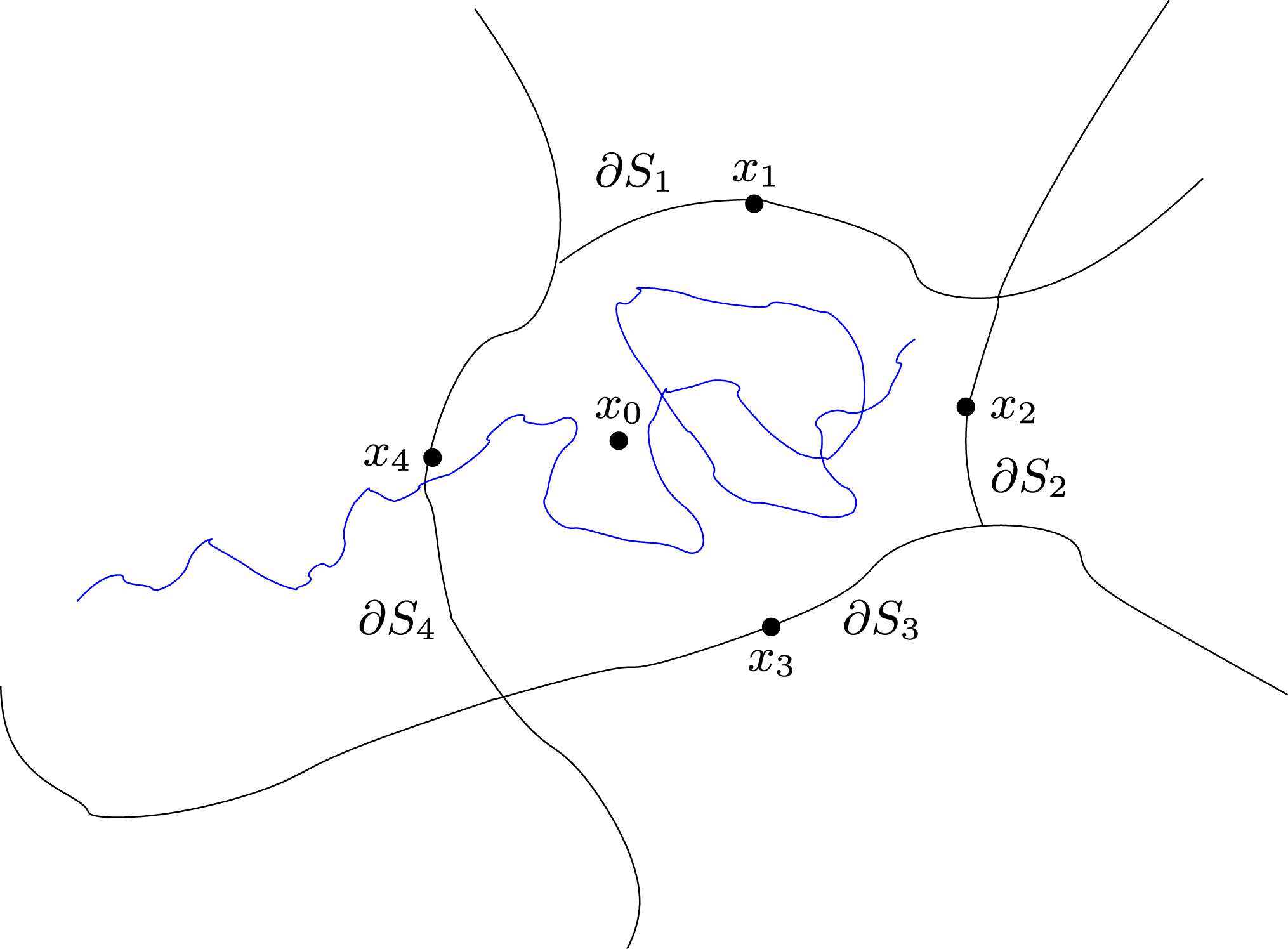
Consider the exit event from  $S$, at a given temperature. Using the notation of
Section 6.3, the set
 $S$ is surrounded by
 $I$ neighbouring states. Let
 $\partial S_{i}$ denote the common boundary with the
 $i$th neighbouring state,
 $i\in \{1,\ldots ,I\}$. The sets
 $\partial S_{i}$ thus form a partition of the boundary
 $\partial S$. Introduce, for
 $i\in \{1,\ldots ,I\}$, the saddle point
 $x_{i}\in \partial S_{i}$, which is the point of lowest energy on
 $\partial S_{i}$: in the low-temperature regime, the paths leaving the state
 $S$ through
 $\partial S_{i}$ leave through a neighbourhood of
 $x_{i}$; this can be inferred from results from large deviation theory,
for example those of Freidlin and Wentzell (Reference Freidlin and Wentzell1984). Let us also denote by
 $x_{0}$ the global minimum of
 $V$ on
 $S$; see Figure 6.4
for a schematic representation of the geometry. As explained in
Section 6.3, the interesting
quantities to define the exit events are:
∙ the probability of exiting through
$\partial S_{i}$, given by (see Proposition 6.7),$$\begin{eqnarray}p(i)=\mathbb{P}(q_{{\it\tau}_{S}}\in \partial S_{i})=-\frac{\int _{\partial S_{i}}\partial _{n}u_{1}\,\text{d}{\it\sigma}}{{\it\beta}{\it\lambda}_{1}\int _{S}u_{1}(x)\,\text{d}x}\end{eqnarray}$$∙ the parameter of the exponential random variable
${\it\tau}_{S}$, that is, $$\begin{eqnarray}{\it\lambda}_{1}=1/\mathbb{E}({\it\tau}_{S}).\end{eqnarray}$$


As explained in Section 6.3, one
way to rewrite the exit event is to attach to each exit region  $\partial S_{i}$ (or to each saddle point
 $x_{i}$) a rate
 $k(i)={\it\lambda}_{1}p(i)$, and to consider
 $I$ independent exponential random variables
 ${\it\tau}_{i}$ with parameter
 $k(i)$. The exit event is then given by
(i) the exit time
$\min _{i\in \{1,\ldots I\}}({\it\tau}_{i})\stackrel{{\mathcal{L}}}{=}{\it\tau}_{S}$, and(ii) the exit region
$\text{arg\,min}_{i\in \{1,\ldots I\}}({\it\tau}_{i})$,


since, for  $i\in \{1,\ldots ,I\}$,
 $$\begin{eqnarray}\mathbb{P}\biggl(\text{arg\,min}_{j\in \{1,\ldots I\}}({\it\tau}_{j})=i\biggr)=p(i).\end{eqnarray}$$
The TAD algorithm requires as an input an approximate expression
of the rate  $k(i)$, namely the Arrhenius law (see (2.83) and recall that the spectrum of
 $-{\mathcal{L}}$ is
 ${\it\beta}$ times the formula given in (2.83))
 $$\begin{eqnarray}k(i)={\it\lambda}_{1}p(i)\simeq {\it\eta}_{i}\exp (-{\it\beta}[V(x_{i})-V(x_{0})]),\end{eqnarray}$$
where  ${\it\eta}_{i}$ is a prefactor independent of
 ${\it\beta}$. In the original paper by Sorensen and Voter (Reference Sorensen and Voter2000), the Arrhenius law is justified using
the (harmonic) transition state theory.
Let us now go back to the TAD algorithm. Using the underlying kinetic Monte Carlo model presented above, and in view of the Arrhenius law (6.39), we obtain
 $$\begin{eqnarray}\frac{k^{\text{hi}}(i)}{k^{\text{lo}}(i)}=\frac{{\it\lambda}_{1}^{\text{hi}}p^{\text{hi}}(i)}{{\it\lambda}_{1}^{\text{lo}}p^{\text{lo}}(i)}\simeq \exp (-({\it\beta}^{\text{hi}}-{\it\beta}^{\text{lo}})(V(x_{i})-V(x_{0})))\end{eqnarray}$$
where, with obvious notation,  ${\it\beta}^{\text{lo}}$ denotes the inverse low temperature,
 ${\it\beta}^{\text{hi}}$ the inverse high temperature, and the superscripts
‘lo’ and ‘hi’ refer to the associated
quantities at low and high temperature, respectively. The extrapolation formula
(6.40) is used in TAD in
order to infer the exit event at low temperature from the exit events observed at
high temperature, by using the formula
 $$\begin{eqnarray}({\it\tau}_{1}^{\text{lo}},\ldots ,{\it\tau}_{I}^{\text{lo}})\stackrel{{\mathcal{L}}}{=}({\rm\Theta}^{1}{\it\tau}_{1}^{\text{hi}},\ldots ,{\rm\Theta}^{I}{\it\tau}_{I}^{\text{hi}}),\end{eqnarray}$$
where
 $$\begin{eqnarray}{\rm\Theta}^{i}=\frac{k^{\text{hi}}(i)}{k^{\text{lo}}(i)}\simeq \exp (-({\it\beta}^{\text{hi}}-{\it\beta}^{\text{lo}})(V(x_{i})-V(x_{0})))\end{eqnarray}$$
is a multiplicative factor constructed from the ratio of the rates
(6.40). In the equality in
law (6.41), the
random variables  ${\it\tau}_{i}^{\text{hi/\text{lo}}}$ are, as described above, exponential random variables with
parameter
 $k^{\text{hi/\text{lo}}}(i)$. To have analytical formulae for the correction factors
 ${\rm\Theta}_{i}$ and make the algorithm practical, the Arrhenius law is assumed
to be exact, and in practice one uses
 $$\begin{eqnarray}{\rm\Theta}^{i}=\exp (-({\it\beta}^{\text{hi}}-{\it\beta}^{\text{lo}})(V(x_{i})-V(x_{0}))).\end{eqnarray}$$
The TAD algorithm thus consists in running the dynamics at high temperature,
observing the exit events through the saddle points on the boundary of the
state,Footnote 21 and updating the exit time and exit region that would have been
observed at low temperature. More precisely, if exits through the saddle points  $\{s_{1},\ldots ,s_{n}\}\subset \{1,\ldots ,I\}$ have been observed, one computes
 $\min ({\rm\Theta}^{s_{1}}{\it\tau}_{s_{1}}^{\text{hi}},\ldots ,{\rm\Theta}^{s_{n}}{\it\tau}_{s_{n}}^{\text{hi}})$ and
 $\text{arg\,min}({\rm\Theta}^{s_{1}}{\it\tau}_{s_{1}}^{\text{hi}},\ldots ,{\rm\Theta}^{s_{n}}{\it\tau}_{s_{n}}^{\text{hi}})$ to get the exit time and the exit region at low temperature.
Let us now discuss how to determine the number  $n$ of exit events to be taken into account. The interesting feature
of TAD compared to a brute force saddle point search is that it is not required to
observe exits through all the saddle points in order to obtain a statistically
correct exit event. Indeed, a stopping criterion is introduced to stop the
calculations at high temperature when the extrapolation procedure will no longer
modify the low-temperature exit event (i.e., it will not modify
 $\min ({\rm\Theta}^{s_{1}}{\it\tau}_{s_{1}}^{\text{hi}},\ldots ,{\rm\Theta}^{s_{n}}{\it\tau}_{s_{n}}^{\text{hi}})$, where
 $\{s_{1},\ldots ,s_{n}\}\subset \{1,\ldots ,I\}$ are the saddle points discovered up to the time when the
stopping criterion is fulfilled). This stopping criterion requires us to provide
some a priori knowledge, typically a lower bound on the barriers
 $V(x_{i})-V(x_{0})$, for
 $i\in \{1,\ldots ,I\}$ (there is also a variant using a lower bound on the prefactors
 ${\it\eta}_{i}$ in (6.39)). In
some sense, TAD can be seen as a clever saddle point search, with a rigorous way
to stop the searching procedure.
If the Arrhenius law (6.39) is exactly satisfied, one can check that the TAD algorithm simulates an exit event which is statistically exact. The mathematical question raised by this algorithm is thus to estimate the difference between the ratio of the rates
 $$\begin{eqnarray}\frac{{\it\lambda}_{1}^{\text{hi}}p^{\text{hi}}(i)}{{\it\lambda}_{1}^{\text{lo}}p^{\text{lo}}(i)}\end{eqnarray}$$
and the estimate deduced from the Arrhenius law
 $$\begin{eqnarray}\exp (-({\it\beta}^{\text{hi}}-{\it\beta}^{\text{lo}})(V(x_{i})-V(x_{0})))\end{eqnarray}$$
(see the extrapolation formula (6.40) above). In Aristoff and Lelièvre (Reference Aristoff and Lelièvre2014) we consider as a first step the case of a
one-dimensional potential, where  $S$ is a single well, and we prove that in the limit
 ${\it\beta}^{\text{hi}},{\it\beta}^{\text{lo}}\rightarrow \infty$ with
 ${\it\beta}^{\text{lo}}/{\it\beta}^{\text{hi}}$ fixed,
 $$\begin{eqnarray}\frac{{\it\lambda}^{\text{hi}}p_{i}^{\text{hi}}}{{\it\lambda}^{\text{lo}}p_{i}^{\text{lo}}}=\text{e}^{-({\it\beta}^{\text{hi}}-{\it\beta}^{\text{lo}})(V(x_{i})-V(x_{0}))}\biggl(1+\text{O}\biggl(\displaystyle \frac{1}{{\it\beta}^{\text{hi}}}-\frac{1}{{\it\beta}^{\text{lo}}}\biggr)\biggr).\end{eqnarray}$$
The extension of this result to a high-dimensional setting is a work in progress.
Notice that, compared to Hyperdynamics, TAD is based on an additional assumption,
namely the Arrhenius law. We expect that this implies larger errors for TAD than
for Hyperdynamics: for Hyperdynamics the error in (6.37)–(6.38) is exponentially small in the limit  ${\it\beta}\rightarrow \infty$, while for TAD, the error scales like
 $1/{\it\beta}$ in (6.42).
However, the interest of TAD compared to Hyperdynamics is that it does not require
a biasing potential, which may be complicated to build in some situations.
6.4.5 Concluding remarks and discussion
This section has given some elements on the analysis of three algorithms that were proposed by A. F. Voter and his co-workers in order to efficiently generate the state-to-state dynamics associated with a metastable stochastic process. The analysis is based on the notion of quasi-stationary distribution (QSD). As explained above, starting from the QSD within a well, the exit event is Markovian since the exit time is exponentially distributed and independent of the next visiting state. From a theoretical viewpoint, the QSD thus seems to be an interesting way to relate Markovian dynamics in continuous state spaces (such as Langevin dynamics (1.9) or overdamped Langevin dynamics (1.8)) with Markovian dynamics in discrete state spaces (kinetic Monte Carlo models or Markov state models). It also gives a natural definition of a metastable region (see Lelièvre Reference Lelièvre, Cangiani, Davidchack, Georgoulis, Gorban, Levesley and Tretyakov2013) as a region where the stochastic process reaches local equilibrium, namely the QSD, before exiting. The associated time scales can be used to quantify the metastability of the process (see after Theorem 4.6 for a related discussion of the quantification of metastability using an alternative approach, namely logarithmic Sobolev inequalities).
Going from Parallel Replica to Hyperdynamics to TAD, the assumptions required for
the algorithm to consistently sample the state-to-state dynamics are ever more
stringent. Indeed, for Parallel Replica, no assumptions are required beyond the
fact that a good estimate of  $t_{\text{corr}}$ is available (to assess the convergence of the QSD).
Hyperdynamics requires additional assumptions on the potential: the metastability
of the state should come from energetic barriers (at least for our mathematical
analysis to apply). Finally, the TAD algorithm also requires the Arrhenius law to
be satisfied. Likewise, going from Parallel Replica to Hyperdynamics to TAD, the
errors introduced by the algorithm are expected to be ever larger. On the other
hand, the expected computational gain with Parallel Replica is typically smaller
than for the two other methods. In addition, comparing Hyperdynamics with TAD, the
advantage of TAD is that it does not require the construction of a biasing
potential, which is a difficult task in general.
We would like to stress that all these algorithms are used in practice with Langevin dynamics (1.9). The mathematical results presented above assume that the dynamics is overdamped Langevin (1.8). Further work is required to extend these results to Langevin dynamics.
6.5 Conclusion: other algorithms and other mathematical frameworks for studying reactive trajectories
In the previous subsections we focused on importance sampling and control techniques to sample reactive paths (see Section 6.2) and on accelerated dynamics techniques to sample exit events from a metastable state (see Section 6.4). As mentioned in the introduction to Section 6, there are in fact many other relevant methods for studying dynamical properties. For the sake of completeness, let us mention a few of them.
For the analysis and sampling of reactive paths and transitions between two metastable states that are a priori fixed, one can mention the following.
∙ Local search techniques. Starting from an initial guess, these methods look for transition paths through an iterative procedure on paths (in the spirit of local optimization methods). For example, let us mention the nudged elastic band (Jónsson, Mills and Jacobsen Reference Jónsson, Mills, Jacobsen, Berne, Ciccotti and Coker1998), the string method (E et al. Reference E, Ren and Vanden-Eijnden2002, Reference E, Ren and Vanden-Eijnden2005), and the max flux approach (Zhao, Shen and Skeel Reference Zhao, Shen and Skeel2010). These techniques aim to find one typical representative path (the minimum energy path or minimum free energy path). Let us also mention transition path sampling methods (Dellago, Bolhuis and Chandler Reference Dellago, Bolhuis and Chandler1999, Dellago and Bolhuis Reference Dellago and Bolhuis2009), which sample transition paths starting from an initial guess using a Metropolis–Hastings algorithm in path space.
∙ Global search, ensemble of trajectories. Other approaches aim at sampling the ensemble of paths joining two metastable states, without any initial guess (in the spirit of global optimization methods). Examples include splitting techniques over ensembles of paths such as the adaptive multilevel splitting method (Cérou and Guyader Reference Cérou and Guyader2007, Cérou et al. Reference Cérou, Guyader, Lelièvre and Pommier2011, Bréhier et al. Reference Bréhier, Gazeau, Goudenège, Lelièvre and Rousset2016), transition interface sampling (van Erp et al. Reference van Erp, Moroni and Bolhuis2003, van Erp and Bolhuis Reference van Erp and Bolhuis2005), forward flux sampling (Allen et al. Reference Allen, Warren and ten Wolde2005, Reference Allen, Valeriani and ten Wolde2009), milestoning techniques (Faradjian and Elber Reference Faradjian and Elber2004, Maragliano, Vanden-Eijnden and Roux Reference Maragliano, Vanden-Eijnden and Roux2009, Schütte et al. Reference Schütte, Noé, Lu, Sarich and Vanden-Eijnden2011), and the associated transition path theory, which gives a nice mathematical framework (E and Vanden-Eijnden Reference E and Vanden-Eijnden2004, Vanden-Eijnden et al. Reference Vanden-Eijnden, Venturoli, Ciccotti and Elber2008, Lu and Nolen Reference Lu and Nolen2015).
There are also techniques which consist in looking for all the local minima and saddle points of the potential energy function, and then building from that a Markov state model using the Arrhenius law (6.39). Examples of saddle point search techniques are the dimer method (Henkelman and Jónsson Reference Henkelman and Jónsson1999, Zhang and Du Reference Zhang and Du2012), activation relaxation techniques (Barkema and Mousseau Reference Barkema and Mousseau1996, Mousseau and Barkema Reference Mousseau and Barkema1998), or gentlest ascent dynamics (Samanta and E Reference Samanta and E2012). This can be used to explore very complicated landscapes: see Wales (Reference Wales2003).
Acknowledgement
This work is supported by the European Research Council via the European Union’s Seventh Framework Programme (FP/2007-2013) and ERC Grant Agreement number 614492, and by the Agence Nationale de la Recherche under grant ANR-14-CE23-0012 (COSMOS). We have also benefited from the scientific environment of the Laboratoire International Associé linking the Centre National de la Recherche Scientifique and the University of Illinois at Urbana-Champaign. We would like to thank all our co-authors on these subjects, and those colleagues who read a preliminary version of the manuscript: Charles-Edouard Bréhier, Eric Cancès, Giacomo Di Gesu, Max Fathi, Carsten Hartmann, Claude Le Bris, Dorian Le Peutrec, Julien Reygner, Julien Roussel, Mathias Rousset, Marielle Simon, Zofia Trstanova, Jonathan Weare, Marcus Weber and Pierre-André Zitt.