2 Materials and methods

Let $y(x)$ be an unknown univariate real-valued function over $[a, b]$ and let $[x_{i-1},x_i],~i=1,2,\ldots ,k,$ be a uniform partition of the interval with mesh length

$$ \begin{align*} h=\frac{b-a}{k}. \end{align*} $$

Assume that the function values

$$ \begin{align*} y_i=y(x_i) \end{align*} $$

are not given, but the integral values $I_i$ of $y(x)$ are known on the k subintervals $[x_{i-1}, x_{i}]$ . Our task is to determine an integro spline $S(x)$ such that

(2.1) $$ \begin{align} \int\limits ^{x_{i}}_{x_{i-1}}S(x)\,dx=\int\limits ^{x_{i}}_{x_{i-1}}y(x)\,dx=I_i, \quad i=1,2,\ldots,k. \end{align} $$

We assume that at least one of $I_i$ is nonzero. Hence, the integro spline $S(x)$ is not identically equal to zero on $[a,b]$ . This type of problem has many practical applications in statistics, numerical analysis, the fields of mechanics and so on. Particularly, Schoenberg [Reference Schoenberg12, p. 115] showed the existence of a cubic/quintic spline $S(x)$ that satisfies the cumulative sequence $S(0)=0$ ,

$$ \begin{align*} S(i)=\sum_{j=1}^iI_j, \end{align*} $$

with suitable end conditions and, letting

$$ \begin{align*} \sigma(x)=S'(x), \end{align*} $$

proved that $\sigma (x)$ is a quadratic/quartic histospline, which is a solution of the problem (2.1). In general, any solution to problem (2.1) is in fact the derivative of a one-degree-higher spline interpolant defined by the cumulative sequence. We now consider a method to find the solution of (2.1) from a given one-degree-higher or -lower solution of (2.1).

We will use the following notation: denote by $S_m(x)$ an integro spline with degree m satisfying (2.1), by $S^{(r)}_m(x)$ the rth derivative of $S_m(x)$ , by $S^{(r)}_m(x_i)$ values of $S^{(r)}_m(x)$ at the knots and by $\tilde {S}^{(r)}_m(x_i)$ specific approximate values for the rth derivative integro spline. Also, $\skew3\hat {S}_m(x)$ is called a local integro spline whose coefficients are explicitly determined by integral values of $I_i$ in a neighbourhood of $x_i$ , without solving any system of equations. Lang and Xu [Reference Lang and Xu10, Reference Xu and Lang18] studied the approximation properties of integro splines under the strong restriction $y\in C^\infty [a,b]$ , but, in this study, we assume that an approximation function y belongs to $C^{m+2}[a,b]$ for the integro spline with degree m. For $y\in C^{m+2}[a,b], m=2,4,6,\ldots ,$ by Taylor expansion of y,

(2.2) $$ \begin{align} I_{i}+I_{i+1}=2\sum\limits_{j=0}^{m/2}\frac{h^{2j+1}}{(2j+1)!}y_i^{(2j)}+O(h^{m+3}), \end{align} $$

where

$$ \begin{align*} y^{(r)}_i=y^{(r)}(x_i). \end{align*} $$

Then the following variant of the Euler–Maclaurin integration formula [Reference Sakai and Usmani11] holds.

Lemma 2.1. Let $y\in C^{m+2}[a,b]$ and $m=2,4,\ldots .$ Then

(2.3) $$ \begin{align} y_i&=l_1\frac1h(I_{i}+I_{i+1})+l_2h(y^{\prime}_{i+1}-y^{\prime}_{i-1})+l_3h^3(y^{\prime\prime\prime}_{i+1}-y^{\prime\prime\prime}_{i-1})+\cdots \notag\\ &\quad +l_{m/2+1}h^{m-1}(y^{(m-1)}_{i+1}-y^{(m-1)}_{i-1})+O(h^{m+2}), \end{align} $$

where

(2.4) $$ \begin{align} &l_1=\frac{1}{2},\notag\\ &l_2=-l_1\frac{1}{3!}=-\frac{1}{12},\notag\\ &l_3=-\bigg(l_2\frac{1}{3!}+l_1\frac{1}{5!}\bigg)=\frac{7}{720},\notag\\ &l_4=-\bigg(l_3\frac{1}{3!}+l_2\frac{1}{5!}+l_1\frac{1}{7!}\bigg)=-\frac{31}{30~240},\notag\\ &\cdots \notag\\ &l_{m/2+1}=-\bigg(l_{m/2}\frac{1}{3!}+l_{m/2-1}\frac{1}{5!}+\cdots+l_2\frac{1}{(m-1)!}+l_1\frac{1}{(m+1)!}\bigg). \end{align} $$

Proof. The proof is by induction on m. When $m=2$ , substituting

$$ \begin{align*} y^{\prime}_{i+1}-y^{\prime}_{i-1}=2hy^{\prime\prime}_i+O(h^3) \end{align*} $$

into (2.2),

$$ \begin{align*} y_i=\frac1{2h}(I_i+I_{i+1})-\frac{h}{12}(y^{\prime}_{i+1}-y^{\prime}_{i-1})+O(h^4), \end{align*} $$

so (2.3) and (2.4) are true for $m=2$ . Suppose that (2.3) and (2.4) are true for $m-2$ . Then, for m, using the Taylor expansion,

(2.5) $$ \begin{align} y^{\prime}_{i+1}-y^{\prime}_{i-1}&=2hy^{\prime\prime}_i+2\frac{h^3}{3!}y_i^{(4)}+\cdots +2\frac{h^{m-1}}{(m-1)!}y^{(m)}_i+O(h^{m+1}),\notag\\ y^{\prime\prime\prime}_{i+1}-y^{\prime\prime\prime}_{i-1}&=2hy^{(4)}_i+2\frac{h^3}{3!}y_i^{(6)}+\cdots +2\frac{h^{m-3}}{(m-3)!}y^{(m)}_i+O(h^{m-1}),\notag\\ &\quad\cdots \notag\\ y^{(m-1)}_{i+1}-y^{(m-1)}_{i-1}&=2hy^{(m)}_i+O(h^{3}). \end{align} $$

Applying the induction hypothesis to (2.5),

(2.6) $$ \begin{align} y^{\prime\prime}_i&=l_1\frac1h(y^{\prime}_{i+1}-y^{\prime}_{i-1})+l_2h(y^{\prime\prime\prime}_{i+1}-y^{\prime\prime\prime}_{i-1})+\cdots\notag\\ &\quad+l_{m/2}h^{m-3}(y^{(m-1)}_{i+1}-y^{(m-1)}_{i-1})+O(h^{m}),\notag\\ y^{(4)}_i&=l_1\frac1h(y^{\prime\prime\prime}_{i+1}-y^{\prime\prime\prime}_{i-1})+l_2h(y^{(5)}_{i+1}-y^{(5)}_{i-1})+\cdots\notag\\ &\quad+l_{m/2-1}h^{m-5}(y^{(m-1)}_{i+1}-y^{(m-1)}_{i-1})+O(h^{m-2}),\notag\\ &\quad\cdots\notag\\ y^{(m)}_i&=l_1\frac1h(y^{(m-1)}_{i+1}-y^{(m-1)}_{i-1})+O(h^{2}). \end{align} $$

Substituting (2.6) into (2.2), we obtain (2.3) with the coefficients (2.4). Hence, (2.3) and (2.4) hold for m, which completes the proof.

The purpose of the equations (2.7) and (2.8) is to determine specific approximate values for $S_m^{(m-1)}(x_i)$ in the cases m even and odd. The Taylor expansion of $S_m(x)$ at the point $x=x_i$ for $m=2,3,4,\ldots $ is

$$ \begin{align*} \begin{aligned} S_m(x)&=S_m(x_i)+(x-x_i)S^{\prime}_m(x_i)+\frac{(x-x_i)^2}{2}S^{\prime\prime}_m(x_i)\\ &\quad +\frac{(x-x_i)^3}{6}S^{\prime\prime\prime}_m(x_i)+\cdots+\frac{(x-x_i)^m}{m!}S^{(m)}_m(x^-_{i}), \end{aligned} \end{align*} $$

where we define the left derivative at $x_i$

$$ \begin{align*} S^{(m)}_m(x^-_{i})=\frac1h(S^{(m-1)}_m(x_{i})-S^{(m-1)}_m(x_{i-1})), \quad x\in [x_{i-1},x_{i}]. \end{align*} $$

Using the last expansion and (2.1) for $i=1,2,\ldots ,k-1$ ,

(2.7) $$ \begin{align} I_i+I_{i+1}&=2hS_m(x_i)+2\frac{h^{3}}{3!}S^{\prime\prime}_m(x_i)+2\frac{h^5}{5!}S^{(4)}_m(x_i)+\cdots \nonumber \\ &\quad +\frac{h^{m+1}}{(m+1)!}(S^{(m)}_m(x^-_{i})+S^{(m)}_m(x^+_{i})) \end{align} $$

and

(2.8) $$ \begin{align} I_{i+1}-I_{i}&=2\frac{h^2}{2!}S^{\prime}_m(x_i)+2\frac{h^4}{4!}S^{\prime\prime\prime}_m(x_i)+\cdots \nonumber \\ &\quad +\frac{h^{m+1}}{m!}(S^{(m)}_m(x^+_i)-S^{(m)}_m(x^-_i)). \end{align} $$

Dropping the last small terms in (2.7) and (2.8), we can find $S^{(m-1)}_m(x_i)$ , which will be used later. Performing a similar computation as in the proof of Lemma 2.1, and using

$$ \begin{align*} S^{(m)}_m(x^-_{i})+S^{(m)}_m(x^+_{i})=\frac1h(S^{(m-1)}_m(x_{i+1})-S^{(m-1)}_m(x_{i-1})) \end{align*} $$

in (2.7),

(2.9) $$ \begin{align} S_m(x_i)&=l_1\frac1h(I_{i}+I_{i+1})+l_2h(S^{\prime}_m(x_{i+1})-S^{\prime}_m(x_{i-1})) \nonumber \\ &\quad +l_3h^3(S^{\prime\prime\prime}_m(x_{i+1})-S^{\prime\prime\prime}_m(x_{i-1}))+\cdots \nonumber \\ &\quad +l_{m/2+1}h^{m-1}(S^{(m-1)}_m(x_{i+1})-S^{(m-1)}_m(x_{i-1})), \quad m=2,4,\ldots, \end{align} $$

and

(2.10) $$ \begin{align} S^{\prime}_m(x_i)&=l_1\frac1h(S_m(x_{i+1})-S_m(x_{i-1})) +l_2h(S^{\prime\prime}_m(x_{i+1})-S^{\prime\prime}_m(x_{i-1}))+\cdots \nonumber \\ &\quad +l_{(m+1)/2}h^{m-2}(S^{(m-1)}_m(x_{i+1})-S^{(m-1)}_m(x_{i-1})),\quad m=3,5,\ldots. \end{align} $$

Let $y\in C^{m+2}[a,b]$ ; the Taylor expansions at the point $x_i$ yield

$$ \begin{align*} h^5y^{(4)}_i-\frac{h^6}{2}y^{(5)}_i=E(i)+O(h^7),\quad i=3,4,\ldots,k-2, \end{align*} $$

where

$$ \begin{align*} E(i)=I_{i-2}-4I_{i-1}+6I_{i}-4I_{i+1}+I_{i+2}. \end{align*} $$

Hence,

(2.11) $$ \begin{align} E(i-1)-2E(i)+E(i+1) &=I_{i-3}-6I_{i-2}+15I_{i-1}-20I_{i}+15I_{i+1}-6I_{i+2}+I_{i+3} \nonumber \\ &=h^7y^{(6)}_i-\frac{h^8}{2}y^{(7)}_i+O(h^9),\quad i=4,5,\ldots,k-3. \end{align} $$

Performing a similar computation as (2.11),

(2.12) $$ \begin{align} &I_{i-m/2-1}-(m+2)I_{i- m/2}+\frac {(m+1)(m+2)}{2}I_{i-m/2+1}+\cdots\notag\\ &\quad +\frac {(m+1)(m+2)}{2}I_{i+ m/2-1}-(m+2)I_{i+ m/2}+I_{i+m/2+1}=O(h^{m+3}),\notag\\ &i=\frac m2+2,\ldots,k-\frac m2 -1,\notag\\ &m=2,4,\ldots, \end{align} $$

where the coefficients can be defined as the coefficients of $x^i$ in the expansion of $(1-x)^{m+2}$ .

3 General algorithm for local integro splines

The properties of the super-convergence of $S^{(r)}_m(x_i)$ proved in the literature [Reference Lang and Xu10, Reference Wu and Zhang16, Reference Wu and Zhang17] suggest the following conjectures.

Conjecture 3.1 If we use a similar technique as in [Reference Wu and Zhang16, Remark 3.1] to construct integro interpolation by B-splines with degrees $m=2,4,\ldots, $ then we conjecture that it possesses the super-convergence property

$$ \begin{align*} \max\limits_{0\leq i\leq k}|S^{(r)}_m(x_i)-y^{(r)}(x_i)|=O(h^{m+2-r}),\quad r=0,2,\ldots,m-2. \end{align*} $$

The super-convergence properties of $S^{\prime }_5(x)$ and $S^{\prime \prime \prime }_5(x)$ of the integro quintic spline are given by Theorem 3.4 in [Reference Zhanlav, Mijiddorj and Behforooz23] as well as those $S^{\prime }_3(x)$ of the integro cubic spline [Reference Zhanlav and Mijiddorj21].

Conjecture 3.2 If we use a convenient technique to construct an integro spline with degrees $m=3,5,\ldots ,$ then we conjecture that it possesses the super-convergence property

$$ \begin{align*} \max\limits_{0\leq i\leq k}|S^{(r)}_m(x_i)-y^{(r)}(x_i)|=O(h^{m+2-r}),\quad r=1,3,\ldots,m-2. \end{align*} $$

Using the notation

$$ \begin{align*} S^{(r)}_m(x_i)=y^{(r)}_i+O(h^{d_r}),~i=0,1,\ldots,k,\quad r=0,1,2,\ldots, \end{align*} $$

and combining the two above-mentioned conjectures, we list the values of $d_r$ of an integro spline with degree m in Table 1.

Table 1

Conjectured values of $d_r$ for $S^{(r)}_m(x_i)$ , $r=0,1,2,\ldots ,~i=0,1,\ldots ,k.$

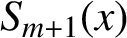
Now, using given specific approximate formulae for the integro spline with degree m, we present a general algorithm to construct a local integro spline with degree $m-1$ or $m+1$ , which provides the values in Table 1. For the general case, let us outline the general algorithm for constructing local integro splines. Suppose that $\skew3\hat {S}_m(x)$ is given. Then $\skew3\hat {S}_{m+1}(x)$ , $m\geq 2$ , is constructed by Algorithm 1.

Let us explain this algorithm when a local integro quartic spline is given by constructing a local integro-sextic spline.

Now, we proceed to construct a local integro-sextic spline.

Thus, we have the Appendix, where we give the errors of $\tilde {S}_6(x)$ at knots.

Theorem 3.4 Let $y\in C^8[a,b]$ and $\tilde {S}_6(x_i)$ be defined by the above IntegroSpline ( $5,\skew3\hat {S}_5(x)$ ). Then the convergence orders of

(3.8) $$ \begin{align} \tilde{S}^{(j)}_6(x_i),\quad i=0,1,\ldots,k,\quad j=0,1,\ldots,5, \end{align} $$

are 8, 6, 6, 4, 4, 2, respectively.

Proof. For $1\leq i+j\leq k$ , using the Taylor expansion of $y\in C^8[a,b]$ at the point $x_i$ ,

(3.9) $$ \begin{align} I_{i+j}&=\int\limits_{x_{i+j-1}}^{x_{i+j}}y(x)dx=\int\limits_{x_{i+j-1}}^{x_{i+j}}\bigg(\sum_{n=0}^7\frac{(x-x_i)^n}{n!}y_i^{(n)}+O(x-x_i)^8\bigg) \,dx\notag \\ &=\sum_{n=1}^8y_i^{(n-1)} \frac{h^n}{n!}(\,j^n-(\,j-1)^n)+O(h^9). \end{align} $$

Substituting (3.9) into the formulae (3.6)–(3.7) as well as the explicit formulae in the Appendix, we obtain (3.8).

In order to construct a local integro-sextic spline using IntegroSpline( $5,\skew3\hat {S}_5(x)$ ), we use the B-spline representation of $S_m(x)$

(3.10) $$ \begin{align} S_m(x)=\sum\limits_{i=1}^{k+m}\alpha_iB_{i,m}(x), \end{align} $$

where $\{B_{i,m},i\in \mathcal {J}\}$ with $\mathcal {J} = \{1,2,\ldots ,k+m\}$ is a basis of the space of splines of degree m and of class $C^{m-1}$ , the support of $B_{i,m}$ being $supp(B_{i,m}) = [x_{i-m-1}, x_i]$ (see, for example, [Reference de Boor, Marsden and Sirovich6, Reference Wang15, Reference Zavyalov, Kvasov and Miroshnichenko19]). As usual, we add multiple knots at the end points $x_{-m} =\cdots =x_{-1}= x_0 = a$ and $b = x_k = x_{k+1} =\cdots = x_{k+m}$ . Using the properties of sextic B-splines when $m=6$ in (3.10),

(3.11) $$ \begin{align} \alpha_{i+4}&=S_6(x_i) + \frac{h}{2}S^{\prime}_6(x_i) -\frac{h^2}{6}S^{\prime\prime}_6(x_i) -\frac{h^3}{8}S^{\prime\prime\prime}_6(x_i) + \frac{h^4 }{90}S^{(4)}_6(x_i)\nonumber \\ &\quad+\frac{h^5}{60} S^{(5)}_6(x_i),\quad i=0,1,\ldots,k. \end{align} $$

From (2.11),

(3.12) $$ \begin{align} I_{i-3}-7I_{i-2}&+21I_{i-1}-35I_{i}+35I_{i+1}-21I_{i+2}+7I_{i+3}-I_{i+4}=O(h^8),\nonumber \\ &i=4,5,\ldots,k-4. \end{align} $$

Substituting the values of $\tilde {S}^{(r)}_6(x_i)$ , $r=0,1,\ldots ,5$ , at the knots into (3.11), and using (3.12), we can find the coefficients $\hat {\alpha }_i$ , $i=4,5,\ldots ,k+4$ , in the local integro-sextic spline,

(3.13) $$ \begin{align} \hat{\alpha}_{i+4}&=\frac1{15120h} (-311I_{i-2}+3168I_{i-1}-14913I_{i}+39232I_{i+1} \notag\\ &\quad -14913I_{i+2}+3168I_{i+3}-311I_{i+4}),\quad i=3,4,\ldots,k-4. \end{align} $$

Hence, the B-spline representation of the local integro-sextic spline is

(3.14) $$ \begin{align} \skew3\hat{S}_6(x)=\sum\limits_{i=1}^{k+6}\hat{\alpha}_iB_{i,6}(x), \end{align} $$

where the coefficients $\hat {\alpha }_i$ are given by (3.13). By virtue of the properties of the sextic B-spline, we have ( $i=0,1,\ldots ,k$ )

(3.15) $$ \begin{align} &\skew3\hat{S}_6(x_i)=\frac{\hat{\alpha}_{i+1}+57\hat{\alpha}_{i+2}+302\hat{\alpha}_{i+3}+302 \hat{\alpha}_{i+4}+57\hat{\alpha}_{i+5}+\hat{\alpha}_{i+6}}{720}, \notag\\ &\skew3\hat{S}^{\prime}_6(x_i)=\frac{-\hat{\alpha}_{i+1}-25\hat{\alpha}_{i+2}-40 \hat{\alpha}_{i+3}+40\hat{\alpha}_{i+4}+25\hat{\alpha}_{i+5}+\hat{\alpha}_{i+6}}{120h},\notag\\ &\skew3\hat{S}^{\prime\prime}_6(x_i)=\frac{\hat{\alpha}_{i+1}+9\hat{\alpha}_{i+2}-10\hat{\alpha}_{i+3}-10 \hat{\alpha}_{i+4}+9\hat{\alpha}_{i+5}+\hat{\alpha}_{i+6}}{24h^2},\notag\\ &\skew3\hat{S}^{\prime\prime\prime}_6(x_i)=\frac{-\hat{\alpha}_{i+1}-\hat{\alpha}_{i+2}+ 8\hat{\alpha}_{i+3}-8\hat{\alpha}_{i+4}+\hat{\alpha}_{i+5}+\hat{\alpha}_{i+6}}{6h^3},\notag\\ &\skew3\hat{S}^{(4)}_6(x_i)=\frac{\hat{\alpha}_{i+1}-3\hat{\alpha}_{i+2}+2\hat{\alpha}_{i+3}+ 2\hat{\alpha}_{i+4}-3\hat{\alpha}_{i+5}+\hat{\alpha}_{i+6}}{2h^4},\notag\\ &\skew3\hat{S}^{(5)}_6(x_i)=\frac{-\hat{\alpha}_{i+1}+5\hat{\alpha}_{i+2}-10\hat{\alpha}_{i+3}+10 \hat{\alpha}_{i+4}-5\hat{\alpha}_{i+5}+\hat{\alpha}_{i+6}}{h^5}. \end{align} $$

From (3.15),

(3.16) $$ \begin{align} \hat{\alpha}_{i+6}-\hat{\alpha}_{i+1}=5h\tilde{S}^{\prime}_6(x_i)+\frac{15h^3\tilde{S}^{\prime\prime\prime}_6(x_i)}{4}+\frac{h^5\tilde{S}^{(5)}_6(x_i)}{3}. \end{align} $$

The remaining coefficients $\hat {\alpha }_i$ of (3.14) for $i = 1,2,3$ and $i =k+ 5,k+ 6$ are determined from (3.11) and (3.16). Thus, we find a local integro-sextic spline $\skew3\hat {S}_6(x)\in C^5[a,b]$ (cf. Figure 1) with (3.14).

Figure 1

$\skew3\hat {S}_6(x)$ (red dots) and $\cos (\pi x)$ (blue dots) on $[0,1]$ , and their derivatives up to fifth order, where $k=80$ . (Colour available online.)

Remark 3.5 If $y\in C^8[a,b]$ , then

$$ \begin{align*} \begin{aligned} &|\tilde{S}^{(r)}_6(x_i)-\skew3\hat{S}^{(r)}_6(x_i)|=O(h^{8-r}),\quad r=0,2,4,\quad i=0,1,\ldots,k,\\ &|\tilde{S}^{(r)}_6(x_i)-\skew3\hat{S}^{(r)}_6(x_i)|=O(h^{7-r}),\quad r=1,3,5. \end{aligned} \end{align*} $$

4 Numerical examples

We present the approximation behaviour (see Table 1 and Theorem 3.4) of $\tilde {S}^{(j)}_6(x_i)$ , $j=0,2,4$ , for given $y\in C^8[0,1]$ as

$$ \begin{align*} y_1(x)=e^x,\quad y_2(x)=\cos(\pi x),\quad y_3(x)=\frac 1{x+2}. \end{align*} $$

Computational results are listed in Tables 2–4. In Tables 2–4, $R_{2r}(k)$ is computed by

$$ \begin{align*} R_{2r}(k)=\max\limits_{0\leq i\leq k}|\skew3\hat{S}^{(2r)}_6(x_i)-y^{(2r)}_j(x_i)|,\quad r=0,1,2,\quad j=1,2,3, \quad \text{and} \end{align*} $$

$$ \begin{align*} \mbox{NCO}=\log_2\bigg|\frac{R_{2r}(k)}{R_{2r}(2k)}\bigg|. \end{align*} $$

The numerical convergence order (NCO) values in Tables 2–4 provide empirical support for the conjectured super-convergence properties. All these computations are carried out using Mathematica, MachinePrecision in 64.

Table 2

Maximum errors of $\skew3\hat {S}_6(x)$ for $y_1(x)=e^x$ .

Table 3

Maximum errors of $\skew3\hat {S}_6(x)$ for $y_2(x)=\cos (\pi x)$ .

Table 4

Maximum errors of $\skew3\hat {S}_6(x)$ for $y_3(x)= 1/(x+2)$ .

Finally, Figure 2 shows the proximity of the constructed spline and the given function histograms.

Figure 2

Functions (blue dots) of integral values in an histogram (blue line) and the plot of the constructed $\skew3\hat {S}_6(x)$ spline (red line), where $k=30$ . (Colour available online.)

The process of integral approximation consisted of two stages: the measurement data were plotted on a grid of rectangular coordinates, the points were connected with a smooth curve and the appropriate formula describing the curve was selected. Then the parameters of the formulae that correspond to the accepted analytical expression were calculated. When constructing an integral approximation, the minimum deviation of one function from another was observed. Comparing the position of the constructed spline and the given function histograms, we can state that there is no oscillation. Also, the horizontal axis is intentionally moved to display the image more clearly.