2.1 Spheroidal inertial pressure modes in aligned rotation

The aligned spheroidal inertial ( $\unicode[STIX]{x1D714}\neq 0$ ) modes can be found by solving Poincaré’s equation (1.13) with $\boldsymbol{f}=\mathbf{0}$ subject to the boundary condition (1.14). Bryan (Reference Bryan1889) following Poincaré (Reference Poincaré1885) transformed Poincaré’s equation, by a (real or imaginary) change of scale in $z$ , to Laplace’s equation which can be solved in prolate or oblate spheroidal coordinates. A different auxiliary set of spheroidal coordinates is used to implement the boundary condition. The two sets of coordinates are confocal and therefore orthogonal, and their angular coordinates coincide (only) on the boundary. The present solution method is to transform the boundary spheroid to a sphere and map the aligned spheroidal problem to a spherical inertial mode problem with modified frequency and boundary condition. In Cartesian coordinates the free Poincaré equation (1.11) with $\boldsymbol{f}=\mathbf{0}$ and $\unicode[STIX]{x1D706}=\text{i}\unicode[STIX]{x1D714}$ is

(2.1) $$\begin{eqnarray}\frac{\unicode[STIX]{x2202}^{2}P}{\unicode[STIX]{x2202}x^{2}}+\frac{\unicode[STIX]{x2202}^{2}P}{\unicode[STIX]{x2202}y^{2}}-\left(\frac{1}{\unicode[STIX]{x1D714}^{2}}-1\right)\frac{\unicode[STIX]{x2202}^{2}P}{\unicode[STIX]{x2202}z^{2}}=0.\end{eqnarray}$$

The scale transformation

(2.2a-c ) $$\begin{eqnarray}{x\unicode[STIX]{x0030A}}=x/a,\quad {y\unicode[STIX]{x0030A}}=y/a,\quad {z\unicode[STIX]{x0030A}}=z/c,\end{eqnarray}$$

maps the boundary spheroid $\unicode[STIX]{x2202}V$ (1.5a ) to the unit sphere ${x\unicode[STIX]{x0030A}}^{2}+{y\unicode[STIX]{x0030A}}^{2}+{z\unicode[STIX]{x0030A}}^{2}=1$ and Poincaré’s equation to

(2.3) $$\begin{eqnarray}\frac{\unicode[STIX]{x2202}^{2}P}{\unicode[STIX]{x2202}{x\unicode[STIX]{x0030A}}^{2}}+\frac{\unicode[STIX]{x2202}^{2}P}{\unicode[STIX]{x2202}{y\unicode[STIX]{x0030A}}^{2}}-\left(\frac{1}{{\unicode[STIX]{x1D714}\unicode[STIX]{x0030A}}^{2}}-1\right)\frac{\unicode[STIX]{x2202}^{2}P}{\unicode[STIX]{x2202}{z\unicode[STIX]{x0030A}}^{2}}=0,\end{eqnarray}$$

if the modified frequency ${\unicode[STIX]{x1D714}\unicode[STIX]{x0030A}}$ is defined by

(2.4) $$\begin{eqnarray}\frac{1}{{\unicode[STIX]{x1D714}\unicode[STIX]{x0030A}}^{2}}-1:=\frac{a^{2}}{c^{2}}\left(\frac{1}{\unicode[STIX]{x1D714}^{2}}-1\right).\end{eqnarray}$$

Thus $|\unicode[STIX]{x1D714}|<1$ from Theorem 1.1(f) implies $|{\unicode[STIX]{x1D714}\unicode[STIX]{x0030A}}|<1$ ; conversely, if $|{\unicode[STIX]{x1D714}\unicode[STIX]{x0030A}}|<1$ , then $|\unicode[STIX]{x1D714}|<1$ ; and $|{\unicode[STIX]{x1D714}\unicode[STIX]{x0030A}}|=1$ if and only if $|\unicode[STIX]{x1D714}|=1$ . Also ${\unicode[STIX]{x1D714}\unicode[STIX]{x0030A}}=0$ if and only if $\unicode[STIX]{x1D714}=0$ , since

(2.5a,b ) $$\begin{eqnarray}{\unicode[STIX]{x1D714}\unicode[STIX]{x0030A}}^{2}:=\frac{(1-e^{2})\unicode[STIX]{x1D714}^{2}}{1-e^{2}\unicode[STIX]{x1D714}^{2}},\quad \unicode[STIX]{x1D714}^{2}:=\frac{{\unicode[STIX]{x1D714}\unicode[STIX]{x0030A}}^{2}}{1-e^{2}(1-{\unicode[STIX]{x1D714}\unicode[STIX]{x0030A}}^{2})},\end{eqnarray}$$

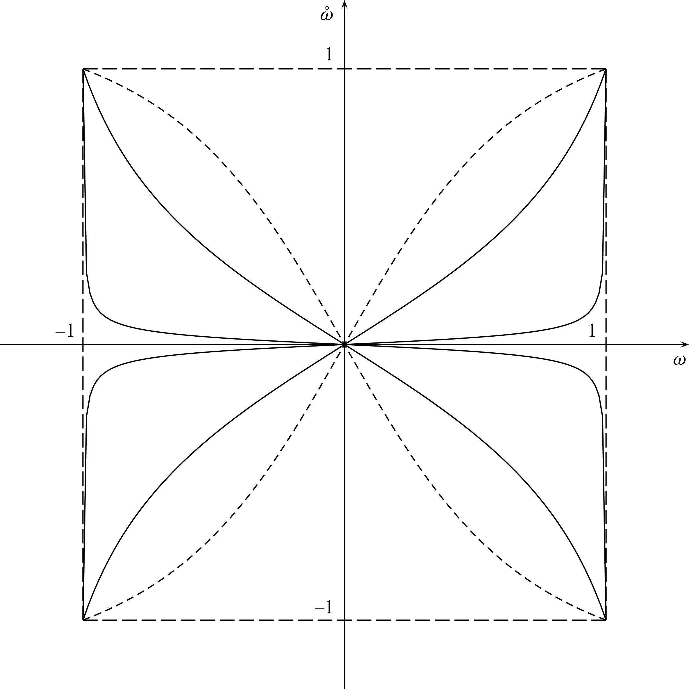
where the oblate ellipticity $e:=\sqrt{1-c^{2}/a^{2}}$ . See figure 1. If the spheroid is oblate $e^{2}>0$ and if prolate $e^{2}<0$ . The prolate ellipticity is $e_{p}:=\sqrt{1-a^{2}/c^{2}}$ , $(1-e^{2})(1-e_{p}^{2})=1$ and $e^{2}=-e_{p}^{2}/(1-e_{p}^{2})$ . Note that there is no distinction between the oblate and prolate cases in the derivation in this section.

Figure 1.

Plot of ${\unicode[STIX]{x1D714}\unicode[STIX]{x0030A}}$ versus $\unicode[STIX]{x1D714}$ for $e=0.8$ , 0.999 and $e_{p}=0.8$ (dashed). By (2.5) the diagram is reflected in the diagonals ${\unicode[STIX]{x1D714}\unicode[STIX]{x0030A}}=\pm \unicode[STIX]{x1D714}$ if $a$ and $c$ are interchanged; this also swaps $e$ and $e_{p}$ . As $e\uparrow 1$ the solid curves are squeezed against the asymptotes $\unicode[STIX]{x1D714}=\pm 1$ and ${\unicode[STIX]{x1D714}\unicode[STIX]{x0030A}}=0$ ; as $e_{p}\uparrow 1$ the dashed curves are squeezed against the asymptotes ${\unicode[STIX]{x1D714}\unicode[STIX]{x0030A}}=\pm 1$ and $\unicode[STIX]{x1D714}=0$ ; see Kudlick (Reference Kudlick1966, pp. 37, 38).

In cylindrical polar coordinates $(s,\unicode[STIX]{x1D719},z)$ the boundary spheroid (1.5a ) is $s^{2}/a^{2}+z^{2}/c^{2}=1$ which, under the scale transformation (2.2), becomes the unit sphere ${s\unicode[STIX]{x0030A}}^{2}+{z\unicode[STIX]{x0030A}}^{2}=1$ , where ${s\unicode[STIX]{x0030A}}=\sqrt{{x\unicode[STIX]{x0030A}}^{2}+{y\unicode[STIX]{x0030A}}^{2}}=s/a$ . Thus from the spherical case (see Ivers et al. Reference Ivers, Jackson and Winch2015) the solutions of Poincaré’s equation are

(2.6) $$\begin{eqnarray}P=P_{n,\unicode[STIX]{x1D714}}^{m}:=P_{n}^{m}(\unicode[STIX]{x1D701}_{{\unicode[STIX]{x1D714}\unicode[STIX]{x0030A}}})\,P_{n}^{m}(\unicode[STIX]{x1D709}_{{\unicode[STIX]{x1D714}\unicode[STIX]{x0030A}}})\text{e}^{\text{i}m\unicode[STIX]{x1D719}},\end{eqnarray}$$

where $(\unicode[STIX]{x1D709},\unicode[STIX]{x1D701},\unicode[STIX]{x1D719})$ are non-orthogonal frequency-dependent spheroidal coordinates (attributed to Greenspan by Kudlick Reference Kudlick1966, equation (4.2)), which are related to scaled cylindrical polar coordinates $({s\unicode[STIX]{x0030A}},\unicode[STIX]{x1D719},{z\unicode[STIX]{x0030A}})$ by

(2.7a-c ) $$\begin{eqnarray}{\unicode[STIX]{x1D70E}\unicode[STIX]{x0030A}}{s\unicode[STIX]{x0030A}}=\sqrt{1-\unicode[STIX]{x1D701}^{2}}\sqrt{1-\unicode[STIX]{x1D709}^{2}},\quad {\unicode[STIX]{x1D714}\unicode[STIX]{x0030A}}{z\unicode[STIX]{x0030A}}=\unicode[STIX]{x1D709}\unicode[STIX]{x1D701},\quad {\unicode[STIX]{x1D70E}\unicode[STIX]{x0030A}}^{2}=1-{\unicode[STIX]{x1D714}\unicode[STIX]{x0030A}}^{2}.\end{eqnarray}$$

In terms of unscaled cylindrical polar coordinates, ${\unicode[STIX]{x1D70E}\unicode[STIX]{x0030A}}s=a\sqrt{1-\unicode[STIX]{x1D701}^{2}}\sqrt{1-\unicode[STIX]{x1D709}^{2}}$ and ${\unicode[STIX]{x1D714}\unicode[STIX]{x0030A}}z=c\unicode[STIX]{x1D709}\unicode[STIX]{x1D701}$ . The element of arc length is given by

(2.8) $$\begin{eqnarray}\displaystyle \text{d}\ell ^{2} & = & \displaystyle \left(\frac{a^{2}}{{\unicode[STIX]{x1D70E}\unicode[STIX]{x0030A}}^{2}}\frac{1-\unicode[STIX]{x1D701}^{2}}{1-\unicode[STIX]{x1D709}^{2}}\unicode[STIX]{x1D709}^{2}+\frac{c^{2}}{{\unicode[STIX]{x1D714}\unicode[STIX]{x0030A}}^{2}}\unicode[STIX]{x1D701}^{2}\right)\text{d}\unicode[STIX]{x1D709}^{2}+\left(\frac{a^{2}}{{\unicode[STIX]{x1D70E}\unicode[STIX]{x0030A}}^{2}}+\frac{c^{2}}{{\unicode[STIX]{x1D714}\unicode[STIX]{x0030A}}^{2}}\right)2\unicode[STIX]{x1D709}\unicode[STIX]{x1D701}\,\text{d}\unicode[STIX]{x1D709}\,\text{d}\unicode[STIX]{x1D701}\nonumber\\ \displaystyle & & \displaystyle +\left(\frac{a^{2}}{{\unicode[STIX]{x1D70E}\unicode[STIX]{x0030A}}^{2}}\frac{1-\unicode[STIX]{x1D709}^{2}}{1-\unicode[STIX]{x1D701}^{2}}\unicode[STIX]{x1D701}^{2}+\frac{c^{2}}{{\unicode[STIX]{x1D714}\unicode[STIX]{x0030A}}^{2}}\unicode[STIX]{x1D709}^{2}\right)\text{d}\unicode[STIX]{x1D701}^{2}+s^{2}\,\text{d}\unicode[STIX]{x1D719}^{2}.\end{eqnarray}$$

In (2.6) $P_{n}^{m}$ is the associated Legendre function of degree $n$ and order $m$ , $m\in \mathbb{Z}$ , $|m|\leqslant n$ , ${\unicode[STIX]{x1D714}\unicode[STIX]{x0030A}}\neq 0$ and the ${\unicode[STIX]{x1D714}\unicode[STIX]{x0030A}}$ dependence of $\unicode[STIX]{x1D701}$ and $\unicode[STIX]{x1D709}$ is indicated.

The spheroidal inertial mode $P_{n,\unicode[STIX]{x1D714}}^{m}$ is a polynomial in $s$ and $z$ of degree $n$ with a $\unicode[STIX]{x1D719}$ -dependent factor $\text{e}^{\text{i}m\unicode[STIX]{x1D719}}$ and a polynomial in $x,y,z$ of degree $n$ (Kudlick Reference Kudlick1966; Zhang et al. Reference Zhang, Earnshaw, Liao and Busse2001). In fact, from Ivers et al. (Reference Ivers, Jackson and Winch2015)

(2.9) $$\begin{eqnarray}P_{n,\unicode[STIX]{x1D714}}^{m}=\left\{\begin{array}{@{}ll@{}}({\unicode[STIX]{x1D70E}\unicode[STIX]{x0030A}}{s\unicode[STIX]{x0030A}}\text{e}^{\text{i}\unicode[STIX]{x1D719}})^{m}({\unicode[STIX]{x1D714}\unicode[STIX]{x0030A}}{z\unicode[STIX]{x0030A}})^{q}U_{n}^{m}({\unicode[STIX]{x1D70E}\unicode[STIX]{x0030A}}^{2}{s\unicode[STIX]{x0030A}}^{2},{\unicode[STIX]{x1D714}\unicode[STIX]{x0030A}}^{2}z^{2}),\quad & \text{if}~m\geqslant 0;\\ ({\unicode[STIX]{x1D70E}\unicode[STIX]{x0030A}}{s\unicode[STIX]{x0030A}}\text{e}^{-\text{i}\unicode[STIX]{x1D719}})^{|m|}({\unicode[STIX]{x1D714}\unicode[STIX]{x0030A}}{z\unicode[STIX]{x0030A}})^{q}U_{n}^{m}({\unicode[STIX]{x1D70E}\unicode[STIX]{x0030A}}^{2}{s\unicode[STIX]{x0030A}}^{2},{\unicode[STIX]{x1D714}\unicode[STIX]{x0030A}}^{2}{z\unicode[STIX]{x0030A}}^{2}),\quad & \text{if}~m<0;\end{array}\right.\end{eqnarray}$$

where $q:=n-|m|\,(\text{mod}~2)$ is either 0 or 1, and $U_{n}^{m}({\unicode[STIX]{x1D70E}\unicode[STIX]{x0030A}}^{2}{s\unicode[STIX]{x0030A}}^{2},{\unicode[STIX]{x1D714}\unicode[STIX]{x0030A}}^{2}{z\unicode[STIX]{x0030A}}^{2})$ is polynomial in ${\unicode[STIX]{x1D70E}\unicode[STIX]{x0030A}}^{2}{s\unicode[STIX]{x0030A}}^{2}$ and ${\unicode[STIX]{x1D714}\unicode[STIX]{x0030A}}^{2}{z\unicode[STIX]{x0030A}}^{2}$ of degree $(n-|m|-q)/2$ . Expressions (2.9) are polynomials in ${x\unicode[STIX]{x0030A}},{y\unicode[STIX]{x0030A}},{z\unicode[STIX]{x0030A}}$ since ${s\unicode[STIX]{x0030A}}\text{e}^{\pm \text{i}\unicode[STIX]{x1D719}}={x\unicode[STIX]{x0030A}}\pm \text{i}{y\unicode[STIX]{x0030A}}$ . The polynomial properties in $s$ , $z$ and in $x$ , $y$ , $z$ follow from ${s\unicode[STIX]{x0030A}}=s/a$ and (2.2). The $z$ -parity of $P_{n,\unicode[STIX]{x1D714}}^{m}$ is determined by  $q$ .

2.2 Frequencies of aligned Coriolis modes

In cylindrical coordinates $(s,\unicode[STIX]{x1D719},z)$ the normal (1.5b ) is $\boldsymbol{n}=s\mathbf{1}_{s}/a^{2}+z\mathbf{1}_{z}/c^{2}$ , and the boundary condition (1.14) becomes in terms of $({s\unicode[STIX]{x0030A}},\unicode[STIX]{x1D719},{z\unicode[STIX]{x0030A}})$ ,

(2.10) $$\begin{eqnarray}{\unicode[STIX]{x1D714}\unicode[STIX]{x0030A}}^{2}{s\unicode[STIX]{x0030A}}\,\unicode[STIX]{x2202}_{{s\unicode[STIX]{x0030A}}}P+({\unicode[STIX]{x1D714}\unicode[STIX]{x0030A}}/\unicode[STIX]{x1D714})\text{i}{\unicode[STIX]{x1D714}\unicode[STIX]{x0030A}}\unicode[STIX]{x2202}_{\unicode[STIX]{x1D719}}P-(1-{\unicode[STIX]{x1D714}\unicode[STIX]{x0030A}}^{2}){z\unicode[STIX]{x0030A}}\,\unicode[STIX]{x2202}_{{z\unicode[STIX]{x0030A}}}P=0.\end{eqnarray}$$

Equation (2.10) differs from the spherical case by the factor ${\unicode[STIX]{x1D714}\unicode[STIX]{x0030A}}/\unicode[STIX]{x1D714}$ in the $\unicode[STIX]{x1D719}$ -derivative term. The boundary condition is transformed to spheroidal coordinates using the following transformations for the first derivatives,

(2.11a,b ) $$\begin{eqnarray}\unicode[STIX]{x2202}_{{s\unicode[STIX]{x0030A}}}P=\frac{\unicode[STIX]{x1D709}\unicode[STIX]{x2202}_{\unicode[STIX]{x1D709}}P-\unicode[STIX]{x1D701}\unicode[STIX]{x2202}_{\unicode[STIX]{x1D701}}P}{{\unicode[STIX]{x1D714}\unicode[STIX]{x0030A}}J},\quad \unicode[STIX]{x2202}_{{z\unicode[STIX]{x0030A}}}P=\frac{\unicode[STIX]{x1D701}(1-\unicode[STIX]{x1D709}^{2})\unicode[STIX]{x2202}_{\unicode[STIX]{x1D709}}P}{{\unicode[STIX]{x1D70E}\unicode[STIX]{x0030A}}^{2}{s\unicode[STIX]{x0030A}}J}-\frac{\unicode[STIX]{x1D709}(1-\unicode[STIX]{x1D701}^{2})\unicode[STIX]{x2202}_{\unicode[STIX]{x1D701}}P}{{\unicode[STIX]{x1D70E}\unicode[STIX]{x0030A}}^{2}{s\unicode[STIX]{x0030A}}J},\end{eqnarray}$$

where $J=\unicode[STIX]{x2202}({s\unicode[STIX]{x0030A}},{z\unicode[STIX]{x0030A}})/\unicode[STIX]{x2202}(\unicode[STIX]{x1D709},\unicode[STIX]{x1D701})=(\unicode[STIX]{x1D701}^{2}-\unicode[STIX]{x1D709}^{2})/({\unicode[STIX]{x1D714}\unicode[STIX]{x0030A}}{\unicode[STIX]{x1D70E}\unicode[STIX]{x0030A}}^{2}{s\unicode[STIX]{x0030A}})$ . The boundary ${s\unicode[STIX]{x0030A}}^{2}+{z\unicode[STIX]{x0030A}}^{2}=1$ is given by ${s\unicode[STIX]{x0030A}}=\sin \unicode[STIX]{x1D703}$ , ${z\unicode[STIX]{x0030A}}=\cos \unicode[STIX]{x1D703}$ or in the spheroidal coordinates $(\unicode[STIX]{x1D709},\unicode[STIX]{x1D701},\unicode[STIX]{x1D719})$ by $\unicode[STIX]{x1D709}=\cos \unicode[STIX]{x1D703}$ , $\unicode[STIX]{x1D701}={\unicode[STIX]{x1D714}\unicode[STIX]{x0030A}}$ . Thus, using (2.11) the boundary condition (2.10) becomes ${\unicode[STIX]{x1D70E}\unicode[STIX]{x0030A}}^{2}\unicode[STIX]{x2202}_{\unicode[STIX]{x1D701}}P-({\unicode[STIX]{x1D714}\unicode[STIX]{x0030A}}/\unicode[STIX]{x1D714})\text{i}\unicode[STIX]{x2202}_{\unicode[STIX]{x1D719}}P=0$ . Substituting the separable solution (2.6) gives $P_{n}^{m}(\unicode[STIX]{x1D709})({\unicode[STIX]{x1D70E}\unicode[STIX]{x0030A}}^{2}\unicode[STIX]{x2202}_{\unicode[STIX]{x1D701}}+m{\unicode[STIX]{x1D714}\unicode[STIX]{x0030A}}/\unicode[STIX]{x1D714})P_{n}^{m}(\unicode[STIX]{x1D701})=0$ on $\unicode[STIX]{x1D709}=\cos \unicode[STIX]{x1D703}$ , $\unicode[STIX]{x1D701}={\unicode[STIX]{x1D714}\unicode[STIX]{x0030A}}$ . Since $\unicode[STIX]{x1D703}$ is arbitrary, ${\unicode[STIX]{x1D714}\unicode[STIX]{x0030A}}$ is a zero of the dispersion relation,

(2.12) $$\begin{eqnarray}(1-{\unicode[STIX]{x1D714}\unicode[STIX]{x0030A}}^{2})\frac{\text{d}P_{n}^{m}({\unicode[STIX]{x1D714}\unicode[STIX]{x0030A}})}{\text{d}{\unicode[STIX]{x1D714}\unicode[STIX]{x0030A}}}+\frac{m{\unicode[STIX]{x1D714}\unicode[STIX]{x0030A}}}{\unicode[STIX]{x1D714}}P_{n}^{m}({\unicode[STIX]{x1D714}\unicode[STIX]{x0030A}})=0.\end{eqnarray}$$

Using the relation (2.5) between $\unicode[STIX]{x1D714}$ and ${\unicode[STIX]{x1D714}\unicode[STIX]{x0030A}}$ condition (2.2) becomes

(2.13) $$\begin{eqnarray}(1-{\unicode[STIX]{x1D714}\unicode[STIX]{x0030A}}^{2})\frac{\text{d}P_{n}^{m}({\unicode[STIX]{x1D714}\unicode[STIX]{x0030A}})}{\text{d}{\unicode[STIX]{x1D714}\unicode[STIX]{x0030A}}}+m\sqrt{1-e^{2}(1-{\unicode[STIX]{x1D714}\unicode[STIX]{x0030A}}^{2})}P_{n}^{m}({\unicode[STIX]{x1D714}\unicode[STIX]{x0030A}})=0.\end{eqnarray}$$

Now (Ivers et al. Reference Ivers, Jackson and Winch2015), $P_{n}^{m}({\unicode[STIX]{x1D714}\unicode[STIX]{x0030A}})=c_{n}^{m}(1-{\unicode[STIX]{x1D714}\unicode[STIX]{x0030A}}^{2})^{|m|/2}\prod _{k=1}^{n-|m|}({\unicode[STIX]{x1D714}\unicode[STIX]{x0030A}}-{\unicode[STIX]{x1D714}\unicode[STIX]{x0030A}}_{k})$ , where ${\unicode[STIX]{x1D714}\unicode[STIX]{x0030A}}_{k}$ for $k=1:n-|m|$ are the $n-|m|$ distinct zeros of $P_{n}^{m}({\unicode[STIX]{x1D714}\unicode[STIX]{x0030A}})$ on $(-1,1)$ and $c_{n}^{m}$ is a constant. The frequency equation (2.13) can be written as

(2.14) $$\begin{eqnarray}\frac{\text{d}\ln P_{n}^{m}({\unicode[STIX]{x1D714}\unicode[STIX]{x0030A}})}{\text{d}{\unicode[STIX]{x1D714}\unicode[STIX]{x0030A}}}=\frac{{\textstyle \frac{1}{2}}|m|}{{\unicode[STIX]{x1D714}\unicode[STIX]{x0030A}}+1}+\frac{{\textstyle \frac{1}{2}}|m|}{{\unicode[STIX]{x1D714}\unicode[STIX]{x0030A}}-1}+\mathop{\sum }_{k=1}^{n-|m|}\frac{1}{{\unicode[STIX]{x1D714}\unicode[STIX]{x0030A}}-{\unicode[STIX]{x1D714}\unicode[STIX]{x0030A}}_{k}}=\sqrt{1-e^{2}(1-{\unicode[STIX]{x1D714}\unicode[STIX]{x0030A}}^{2})}\left[\frac{{\textstyle \frac{1}{2}}m}{{\unicode[STIX]{x1D714}\unicode[STIX]{x0030A}}-1}-\frac{{\textstyle \frac{1}{2}}m}{{\unicode[STIX]{x1D714}\unicode[STIX]{x0030A}}+1}\right].\end{eqnarray}$$

If $m>0$ rearranging the second equation in (2.14) gives

(2.15) $$\begin{eqnarray}\mathop{\sum }_{k=1}^{n-|m|}\frac{1}{{\unicode[STIX]{x1D714}\unicode[STIX]{x0030A}}-{\unicode[STIX]{x1D714}\unicode[STIX]{x0030A}}_{k}}=-\frac{{\textstyle \frac{1}{2}}m[1+\sqrt{1-e^{2}(1-{\unicode[STIX]{x1D714}\unicode[STIX]{x0030A}}^{2})}]}{{\unicode[STIX]{x1D714}\unicode[STIX]{x0030A}}+1}+\frac{{\textstyle \frac{1}{2}}me^{2}({\unicode[STIX]{x1D714}\unicode[STIX]{x0030A}}+1)}{1+\sqrt{1-e^{2}(1-{\unicode[STIX]{x1D714}\unicode[STIX]{x0030A}}^{2})}}<0.\end{eqnarray}$$

The expression on the right-hand side is: monotonic in $|{\unicode[STIX]{x1D714}\unicode[STIX]{x0030A}}|<1$ for fixed $0\leqslant e^{2}<1$ (oblate) or for $-\infty <e^{2}\leqslant 0$ (prolate); tends to $-\infty$ as ${\unicode[STIX]{x1D714}\unicode[STIX]{x0030A}}\rightarrow -1+$ or to $-(1/2)m(1-e^{2})$ as ${\unicode[STIX]{x1D714}\unicode[STIX]{x0030A}}\rightarrow 1-$ ; and is monotonic in $-\infty <e^{2}<1$ for fixed ${\unicode[STIX]{x1D714}\unicode[STIX]{x0030A}}$ . For $m<0$ the signs of the terms on the right-hand side of (2.15) are changed and ${\unicode[STIX]{x1D714}\unicode[STIX]{x0030A}}$ is replaced by $-{\unicode[STIX]{x1D714}\unicode[STIX]{x0030A}}$ . 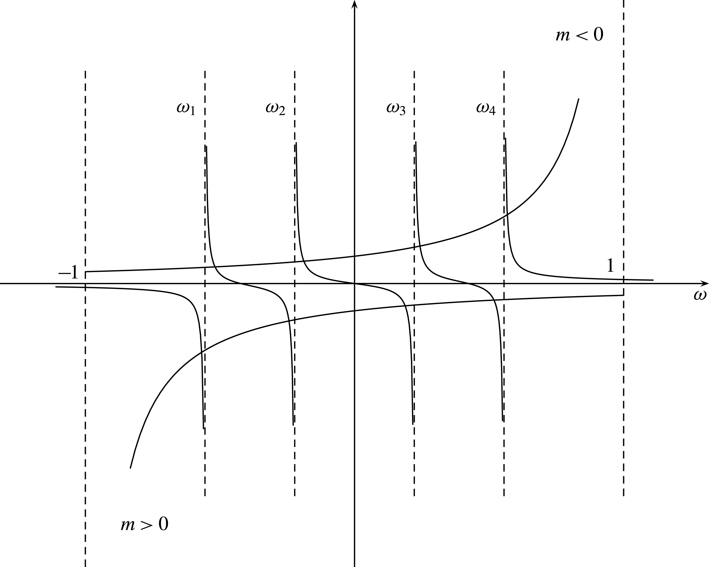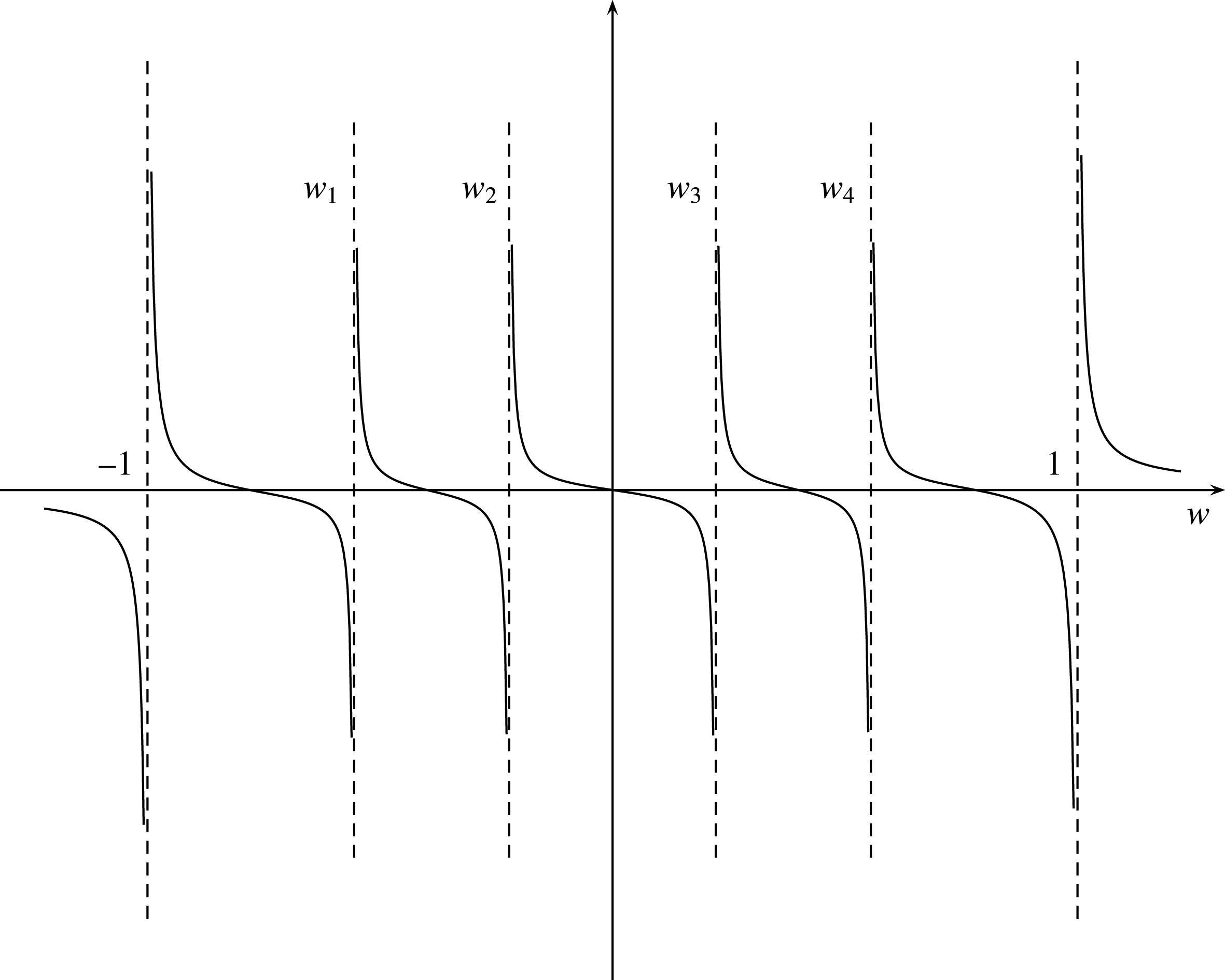Figure 2 shows a schematic plot of the two sides of the second equation in (2.15) for $n-|m|=4$ . For $m\neq 0$ this equation has $n-|m|$ zeros; for $m=0$ there are $n-1$ zeros. The zeros are not symmetrically distributed about ${\unicode[STIX]{x1D714}\unicode[STIX]{x0030A}}=0$ but they are reasonably uniformly distributed on $[-1,1]$ . Thus for extremely oblate (prolate) spheroids with $e\approx 1$ ( $e_{p}\approx 1$ ) the real frequencies are clustered near $\unicode[STIX]{x1D714}=\pm 1$ ( $\unicode[STIX]{x1D714}=0$ ); see figure 2. This result was inferred from computations by Kudlick (Reference Kudlick1966). Geostrophic modes ${\unicode[STIX]{x1D714}\unicode[STIX]{x0030A}}=0$ occur if and only if $m=0$ and $n$ is even. There are no $m=\pm n$ modes: in fact, the dispersion relation gives ${\unicode[STIX]{x1D714}\unicode[STIX]{x0030A}}=1$ ( $-1$ ) for $m>0$ ( ${<}0$ ) in these cases. Thus we label the non-zero frequencies for $0<m\leqslant n-1$ by ${\unicode[STIX]{x1D714}\unicode[STIX]{x0030A}}_{n,j}^{m}$ ( $\unicode[STIX]{x1D714}_{n,j}^{m}$ ), where $j\in \mathbb{Z}$ , $j\neq 0$ and $j=-(n-m+1)/2:(n-m-1)/2$ , if $n-m$ is odd, or $j=-(n-m)/2:(n-m)/2$ if $n-m$ is even. The zero frequencies are ${\unicode[STIX]{x1D714}\unicode[STIX]{x0030A}}_{n,0}^{0}$ , where $n$ is even, $m=0$ and $j=0$ . For $-(n-1)\leqslant m<0$ , ${\unicode[STIX]{x1D714}\unicode[STIX]{x0030A}}_{n,j}^{m}={\unicode[STIX]{x1D714}\unicode[STIX]{x0030A}}_{n,-j}^{-m}$ ( $\unicode[STIX]{x1D714}_{n,j}^{m}=\unicode[STIX]{x1D714}_{n,-j}^{-m}$ ). We define the associated inertial pressure mode for the non-zero frequency $\unicode[STIX]{x1D714}_{n,j}^{m}$ by

(2.16) $$\begin{eqnarray}P_{n,j}^{m}:=P_{n,\unicode[STIX]{x1D714}_{n,j}^{m}}^{m}.\end{eqnarray}$$

Note that $P_{n,j}^{m}=P_{n,-j}^{-m\ast }$ . The aligned geostrophic modes are constructed in § 2.3.

Figure 2.

Schematic plot of (2.16) and the $m>0$ analogue for inertial frequencies $\unicode[STIX]{x1D714}$ with $n-|m|=4$ . The right side curves are labelled by $m>0$ and $m<0$ ; as $e^{2}\uparrow 1$ these curves move toward the $\unicode[STIX]{x1D714}$ axis; and away from the $\unicode[STIX]{x1D714}$ axis as $e^{2}\downarrow -\infty$ . The $m=0$ curve is the $\unicode[STIX]{x1D714}$ axis.

The number of Coriolis pressure modes of degree $N+1$ or less, which equals the number of Coriolis velocity modes of degree $N$ or less, is

(2.17) $$\begin{eqnarray}C_{N}={\textstyle \frac{1}{6}}N(N+1)(2N+7),\end{eqnarray}$$

as (expectedly) in the spherical case. For $N=1,2$ there are 3, 11 modes and for $N\gg 1~C_{N}\approx N^{3}/3$ .

2.3 Aligned geostrophic pressure modes

The natural aligned geostrophic modes, which are hierarchical in polynomial degree, can be constructed by taking the limit $\unicode[STIX]{x1D714}\rightarrow 0$ of the aligned inertial modes (2.7), as in the spherical case.

Lemma 2.1. For $m=0$ and $\unicode[STIX]{x1D714}\rightarrow 0$ the solutions (2.6) reduce to the geostrophic modes,

(2.18) $$\begin{eqnarray}P_{n,0}^{0}(s)=P_{n}(0)P_{n}(\sqrt{1-s^{2}/a^{2}})-[P_{n}(0)]^{2},\end{eqnarray}$$

where $n$ is even. $P_{n,0}^{0}(s)$ is a polynomial of even degree $n$ in $s$ and $P_{n}$ is the Legendre polynomial of degree $n$ . As $s\rightarrow a$ , $P_{n,0}^{0}(s)\rightarrow 0$ . In terms of Jacobi polynomials $P_{n,0}^{0}(s)=(-)^{n/2}P_{n}(0)P_{n/2}^{(-1/2,0)}(2s^{2}/a^{2}-1)-[P_{n}(0)]^{2}$ .

Proof. From (2.7) $\unicode[STIX]{x1D709}^{2}+\unicode[STIX]{x1D701}^{2}=1-{\unicode[STIX]{x1D70E}\unicode[STIX]{x0030A}}^{2}{s\unicode[STIX]{x0030A}}^{2}+(\unicode[STIX]{x1D709}\unicode[STIX]{x1D701})^{2}=1-{\unicode[STIX]{x1D70E}\unicode[STIX]{x0030A}}^{2}{s\unicode[STIX]{x0030A}}^{2}+{\unicode[STIX]{x1D714}\unicode[STIX]{x0030A}}^{2}{z\unicode[STIX]{x0030A}}^{2}$ . Thus as $\unicode[STIX]{x1D714}\rightarrow 0$ , ${\unicode[STIX]{x1D714}\unicode[STIX]{x0030A}}\rightarrow 0$ by (2.5) and $\unicode[STIX]{x1D709}^{2}+\unicode[STIX]{x1D701}^{2}\rightarrow 1-{s\unicode[STIX]{x0030A}}^{2}=1-s^{2}/a^{2}$ . Further, by rearranging the binomial expansion of $(\unicode[STIX]{x1D709}^{2}+\unicode[STIX]{x1D701}^{2})^{l}$ into the form,

(2.19) $$\begin{eqnarray}\unicode[STIX]{x1D709}^{2l}+\unicode[STIX]{x1D701}^{2l}=(\unicode[STIX]{x1D709}^{2}+\unicode[STIX]{x1D701}^{2})^{l}-\mathop{\sum }_{j=1}^{\lfloor (l-1)/2\rfloor }\!\;\text{}^{l}C_{j}(\unicode[STIX]{x1D709}\unicode[STIX]{x1D701})^{2j}(\unicode[STIX]{x1D709}^{2(l-2j)}+\unicode[STIX]{x1D701}^{2(l-2j)}),\end{eqnarray}$$

$\unicode[STIX]{x1D709}^{2l}+\unicode[STIX]{x1D701}^{2l}\rightarrow (\unicode[STIX]{x1D709}^{2}+\unicode[STIX]{x1D701}^{2})^{l}$ , since ${\unicode[STIX]{x1D70E}\unicode[STIX]{x0030A}}\rightarrow 1$ and $(\unicode[STIX]{x1D709}\unicode[STIX]{x1D701})^{2}={\unicode[STIX]{x1D714}\unicode[STIX]{x0030A}}^{2}{z\unicode[STIX]{x0030A}}^{2}\rightarrow 0$ . If $n$ is even, $P_{n}(z)=\sum _{k=0}^{n/2}p_{n,2k}z^{2k}$ , where the $p_{n,2k}$ are constants, and

(2.20) $$\begin{eqnarray}P_{n}(\unicode[STIX]{x1D709})P_{n}(\unicode[STIX]{x1D701})=p_{n,0}\left[\mathop{\sum }_{k=0}^{n/2}p_{n,2k}(\unicode[STIX]{x1D709}^{2k}+\unicode[STIX]{x1D701}^{2k})-p_{n,0}\right]+(\unicode[STIX]{x1D709}\unicode[STIX]{x1D701})^{2}\mathop{\sum }_{k=1}^{n/2}\mathop{\sum }_{l=1}^{n/2}p_{n,2k}p_{l,2k}\unicode[STIX]{x1D709}^{2(k-1)}\unicode[STIX]{x1D701}^{2(l-1)}.\end{eqnarray}$$

The double sum is $O(\unicode[STIX]{x1D709}\unicode[STIX]{x1D701})^{2}$ . Thus for $n$ even, $P_{n}(\unicode[STIX]{x1D709})P_{n}(\unicode[STIX]{x1D701})\rightarrow P_{n,0}^{0}$ in (2.18) as $\unicode[STIX]{x1D714}\rightarrow 0$ , since $p_{n,0}=P_{n}(0)$ . If $n$ is odd, $P_{n}(\unicode[STIX]{x1D709})P_{n}(\unicode[STIX]{x1D701})\rightarrow 0$ as $\unicode[STIX]{x1D714}\rightarrow 0$ .◻

The modes (2.18) are orthogonal, for evaluating the inner product $(\boldsymbol{v}_{1},\boldsymbol{v}_{2})$ of two geostrophic modes gives

(2.21) $$\begin{eqnarray}(\boldsymbol{v}_{1},\boldsymbol{v}_{2})=\int _{V}\unicode[STIX]{x1D735}P_{1}\boldsymbol{\cdot }\unicode[STIX]{x1D735}P_{2}^{\ast }\,\text{d}V,\end{eqnarray}$$

noting $n_{1}$ and $n_{2}$ are even and substituting $v^{2}=1-s^{2}/a^{2}$ yields, apart from the factor $P_{n_{1}}(0)P_{n_{2}}(0)$ ,

(2.22) $$\begin{eqnarray}\int _{V}\unicode[STIX]{x1D735}P_{n_{1}}(\sqrt{1-s^{2}/a^{2}})\boldsymbol{\cdot }\unicode[STIX]{x1D735}P_{n_{2}}(\sqrt{1-s^{2}/a^{2}})\,\text{d}V=2\unicode[STIX]{x03C0}c\int _{-1}^{1}P_{n_{1}}^{\prime }(v)(1-v^{2})P_{n_{2}}^{\prime }(v)\,\text{d}v.\end{eqnarray}$$

An integration by parts and Legendre’s differential equation shows the last integral vanishes if $n_{1}\neq n_{2}$ .

2.4 Aligned velocity modes

The velocity modes are constructed from the pressure modes using (3.9). Thus associated with the pressure mode $P_{n+1,j}^{m}$ is the velocity mode $\boldsymbol{v}_{n,j}^{m}$ . Define

(2.23) $$\begin{eqnarray}\boldsymbol{v}_{n}^{m}(\unicode[STIX]{x1D714}):=\left\{\begin{array}{@{}l@{}}\displaystyle \frac{\text{i}\unicode[STIX]{x1D714}}{1-\unicode[STIX]{x1D714}^{2}}(\unicode[STIX]{x1D735}P_{n+1,\unicode[STIX]{x1D714}}^{m}-\unicode[STIX]{x1D714}^{-2}\widehat{\unicode[STIX]{x1D734}}\widehat{\unicode[STIX]{x1D734}}\boldsymbol{\cdot }\unicode[STIX]{x1D735}P_{n+1,\unicode[STIX]{x1D714}}^{m})+\frac{1}{1-\unicode[STIX]{x1D714}^{2}}\widehat{\unicode[STIX]{x1D734}}\times \unicode[STIX]{x1D735}P_{n+1,\unicode[STIX]{x1D714}}^{m},\quad \unicode[STIX]{x1D714}\neq 0;\quad \\ \widehat{\unicode[STIX]{x1D734}}\times \unicode[STIX]{x1D735}P_{n+1,0}^{0}(s),\quad m=0,n~\text{odd;}\quad \unicode[STIX]{x1D714}=0.\quad \end{array}\right.\end{eqnarray}$$

The Coriolis velocity modes are thus

(2.24) $$\begin{eqnarray}\boldsymbol{v}_{n,j}^{m}:=N_{n,j}^{m}\boldsymbol{v}_{n}^{m}(\unicode[STIX]{x1D714}_{n+1,j}^{m}),\quad |m|\leqslant n,\end{eqnarray}$$

where $j=-(n-m+1)/2:(n-m-1)/2$ if $n-m$ is odd, $j=-(n-m)/2:(n-m)/2$ if $n-m$ is even and $j\neq 0$ unless $m=0$ and $n$ is odd. The normalisation constant $N_{n,j}^{m}>0$ is chosen so that the mode is normalised to $(\boldsymbol{v}_{n,j}^{m},\boldsymbol{v}_{n,j}^{m})=1$ . The complex conjugate $\boldsymbol{v}_{n,j}^{m\ast }=\boldsymbol{v}_{n,-j}^{-m}$ in agreement with Theorem 1.1(f). No modes $\boldsymbol{v}_{n,\unicode[STIX]{x1D714}}^{m}$ arise from $m=n+1$ , i.e. $P_{n+1}^{\pm (n+1)}$ . For $m\neq 0$ the associated inertial waves propagate eastward (westward) if $j>0$ ( $j<0$ ). Equatorial symmetries are determined by $n-m$ : the velocity modes are quadrupole symmetric if $n-m=0\,(\text{mod}~2)$ and dipole symmetric if $n-m=1\,(\text{mod}~2)$ ; and rotational symmetries about $\widehat{\unicode[STIX]{x1D734}}$ are determined by  $m$ . In terms of Jacobi polynomials their $\unicode[STIX]{x1D719}$ -components can be written as

(2.25) $$\begin{eqnarray}v_{2n-1,0}^{0}=N_{2n-1,0}^{0}\frac{\text{d}P_{2n,0}^{0}(s)}{\text{d}s}=N_{2n-1,0}^{0}(-)^{n}(2n+1)P_{2n}(0)sP_{n}^{(1/2,1)}(2s^{2}/a^{2}-1)/a^{2}.\end{eqnarray}$$

Spheroidal Coriolis modes, which are all polynomial flows (see Theorem 6.2), are labelled below using a Greek letter, e.g. $\boldsymbol{v}_{\unicode[STIX]{x1D6FC}}$ ; the degree of $\boldsymbol{v}_{\unicode[STIX]{x1D6FC}}$ is denoted by $\deg \unicode[STIX]{x1D6FC}$ and the angular frequency by $\unicode[STIX]{x1D714}_{\unicode[STIX]{x1D6FC}}$ . For aligned modes the Greek letter denotes a three index, e.g. $\boldsymbol{v}_{\unicode[STIX]{x1D6FC}}\equiv \boldsymbol{v}_{n_{\unicode[STIX]{x1D6FC}},j_{\unicode[STIX]{x1D6FC}}}^{m_{\unicode[STIX]{x1D6FC}}}$ . For tilted modes the three-index interpretation fails but it can be interpreted as a two index: the first index indicates the polynomial degree of the mode and the second labels its frequency.

3.1 A spheroidal toroidal–poloidal basis

Introduce the homoeoidal spheroidal coordinates $(r,\unicode[STIX]{x1D703},\unicode[STIX]{x1D719})$ in dimensionless form,

(3.1a-c ) $$\begin{eqnarray}x=ar\sin \unicode[STIX]{x1D703}\cos \unicode[STIX]{x1D719},\quad y=ar\sin \unicode[STIX]{x1D703}\sin \unicode[STIX]{x1D719},\quad z=cr\cos \unicode[STIX]{x1D703}.\end{eqnarray}$$

Let $\boldsymbol{e}_{r}:=\unicode[STIX]{x2202}_{r}\boldsymbol{r}$ , $\boldsymbol{e}_{\unicode[STIX]{x1D703}}:=\unicode[STIX]{x2202}_{\unicode[STIX]{x1D703}}\boldsymbol{r}/r$ , $\boldsymbol{e}_{\unicode[STIX]{x1D719}}:=\unicode[STIX]{x2202}_{\unicode[STIX]{x1D719}}\boldsymbol{r}/r\sin \unicode[STIX]{x1D703}$ and let the velocity $\boldsymbol{v}=v_{r}\boldsymbol{e}_{r}+v_{\unicode[STIX]{x1D703}}\boldsymbol{e}_{\unicode[STIX]{x1D703}}+v_{\unicode[STIX]{x1D719}}\boldsymbol{e}_{\unicode[STIX]{x1D719}}$ . Define a class of spheroidal toroidal and poloidal fields

(3.2a,b ) $$\begin{eqnarray}\boldsymbol{T}\{t\}:=\boldsymbol{e}_{\unicode[STIX]{x1D703}}\frac{\unicode[STIX]{x2202}_{\unicode[STIX]{x1D719}}t}{\sin \unicode[STIX]{x1D703}}-\boldsymbol{e}_{\unicode[STIX]{x1D719}}\unicode[STIX]{x2202}_{\unicode[STIX]{x1D703}}t,\quad \boldsymbol{S}\{s\}:=-\boldsymbol{e}_{r}\frac{{\unicode[STIX]{x1D6EC}\unicode[STIX]{x0030A}}^{2}s}{r}+\boldsymbol{e}_{\unicode[STIX]{x1D703}}\frac{\unicode[STIX]{x2202}_{\unicode[STIX]{x1D703}}\unicode[STIX]{x2202}_{r}(rs)}{r}+\boldsymbol{e}_{\unicode[STIX]{x1D719}}\frac{\unicode[STIX]{x2202}_{\unicode[STIX]{x1D719}}\unicode[STIX]{x2202}_{r}(rs)}{r\sin \unicode[STIX]{x1D703}},\end{eqnarray}$$

where ${\unicode[STIX]{x1D6EC}\unicode[STIX]{x0030A}}^{2}s:=(\sin \unicode[STIX]{x1D703})^{-1}\unicode[STIX]{x2202}_{\unicode[STIX]{x1D703}}(\sin \unicode[STIX]{x1D703}\unicode[STIX]{x2202}_{\unicode[STIX]{x1D703}}s)+(\sin \unicode[STIX]{x1D703})^{-2}\unicode[STIX]{x2202}_{\unicode[STIX]{x1D719}}\unicode[STIX]{x2202}_{\unicode[STIX]{x1D719}}s$ . Throughout the present § 3, $s$ and $t$ are the poloidal and toroidal potentials, not the cylindrical radius and the time. These fields are solenoidal identically in $t$ and $s$ , $\unicode[STIX]{x1D735}\boldsymbol{\cdot }\boldsymbol{T}\{t\}=0$ and $\unicode[STIX]{x1D735}\boldsymbol{\cdot }\boldsymbol{S}\{s\}=0$ , and any incompressible velocity can be represented as a sum of spheroidal toroidal and poloidal fields, $\boldsymbol{v}=\boldsymbol{S}\{s\}+\boldsymbol{T}\{t\}$ , and the impenetrable boundary condition (2.9) becomes

(3.3) $$\begin{eqnarray}s=0,\quad \text{at}~r=1.\end{eqnarray}$$

The streamlines of the toroidal flow $\boldsymbol{T}\{t\}$ are given by the level contours of $t$ on the surfaces of constant $r$ which are nested homoeoidal spheroids.

Scale the Cartesian coordinates ${x\unicode[STIX]{x0030A}}=x/a$ , ${y\unicode[STIX]{x0030A}}=y/a$ and ${z\unicode[STIX]{x0030A}}=z/c$ , and the velocity,

(3.4a,b ) $$\begin{eqnarray}{\boldsymbol{r}\unicode[STIX]{x0030A}}=\unicode[STIX]{x1D647}\boldsymbol{\cdot }\boldsymbol{r}=\boldsymbol{r}\boldsymbol{\cdot }\unicode[STIX]{x1D647},\quad {\boldsymbol{v}\unicode[STIX]{x0030A}}=\unicode[STIX]{x1D647}\boldsymbol{\cdot }\boldsymbol{v}=\boldsymbol{v}\boldsymbol{\cdot }\unicode[STIX]{x1D647},\end{eqnarray}$$

where ${\boldsymbol{r}\unicode[STIX]{x0030A}}:={x\unicode[STIX]{x0030A}}\boldsymbol{i}+{y\unicode[STIX]{x0030A}}\boldsymbol{j}+{z\unicode[STIX]{x0030A}}\boldsymbol{k}$ is the position vector in $({x\unicode[STIX]{x0030A}},{y\unicode[STIX]{x0030A}},{z\unicode[STIX]{x0030A}})$ -space ${E\unicode[STIX]{x0030A}}^{3}$ , the diagonal scale tensor $\unicode[STIX]{x1D647}:=a^{-1}(\boldsymbol{i}\boldsymbol{i}+\boldsymbol{j}\boldsymbol{j})+c^{-1}\boldsymbol{k}\boldsymbol{k}$ with inverse $\unicode[STIX]{x1D647}^{-1}:=a(\boldsymbol{i}\boldsymbol{i}+\boldsymbol{j}\boldsymbol{j})+c\boldsymbol{k}\boldsymbol{k}$ . Let ${{\mathcal{P}}\unicode[STIX]{x0030A}}_{N}$ denote the set of complex polynomials in $({x\unicode[STIX]{x0030A}},{y\unicode[STIX]{x0030A}},{z\unicode[STIX]{x0030A}})$ of degree $N$ . If $f(\boldsymbol{r})\in {\mathcal{P}}_{N}$ then $f(\unicode[STIX]{x1D647}^{-1}\boldsymbol{\cdot }{\boldsymbol{r}\unicode[STIX]{x0030A}})\in {{\mathcal{P}}\unicode[STIX]{x0030A}}_{N}$ and conversely. Let ${V\unicode[STIX]{x0030A}}:=\{{\boldsymbol{r}\unicode[STIX]{x0030A}}\in {E\unicode[STIX]{x0030A}}^{3}\mid r=|{\boldsymbol{r}\unicode[STIX]{x0030A}}|\leqslant 1\}$ . Define the space of (inviscid) complex polynomial flows of degree $N$ on ${V\unicode[STIX]{x0030A}}$ , ${\boldsymbol{{\mathcal{P}}}\unicode[STIX]{x0030A}}_{N}({V\unicode[STIX]{x0030A}})=\{{\boldsymbol{v}\unicode[STIX]{x0030A}}\in {\mathcal{P}}_{N}^{3}\mid {\unicode[STIX]{x1D735}\unicode[STIX]{x0030A}}\boldsymbol{\cdot }{\boldsymbol{v}\unicode[STIX]{x0030A}}=0~\text{in}~{V\unicode[STIX]{x0030A}},{\boldsymbol{r}\unicode[STIX]{x0030A}}\boldsymbol{\cdot }{\boldsymbol{v}\unicode[STIX]{x0030A}}=0~\text{on}~\unicode[STIX]{x2202}{V\unicode[STIX]{x0030A}}\}$ . By (3.4) ${\unicode[STIX]{x1D735}\unicode[STIX]{x0030A}}\boldsymbol{\cdot }{\boldsymbol{v}\unicode[STIX]{x0030A}}=\unicode[STIX]{x1D735}\boldsymbol{\cdot }\boldsymbol{v}$ and $\boldsymbol{n}=\unicode[STIX]{x1D647}\boldsymbol{\cdot }{\boldsymbol{r}\unicode[STIX]{x0030A}}$ , noting (1.5), and $\boldsymbol{n}\boldsymbol{\cdot }\boldsymbol{v}={\boldsymbol{r}\unicode[STIX]{x0030A}}\boldsymbol{\cdot }{\boldsymbol{v}\unicode[STIX]{x0030A}}$ . Thus ${\boldsymbol{v}\unicode[STIX]{x0030A}}\in {\boldsymbol{{\mathcal{P}}}\unicode[STIX]{x0030A}}_{N}({V\unicode[STIX]{x0030A}})$ if and only if $\boldsymbol{v}\in \boldsymbol{{\mathcal{P}}}_{N}(V)$ .

If $\boldsymbol{v}\in \boldsymbol{{\mathcal{P}}}_{N}(V)$ then ${\boldsymbol{v}\unicode[STIX]{x0030A}}=\unicode[STIX]{x1D647}\boldsymbol{\cdot }\boldsymbol{v}=\unicode[STIX]{x1D647}\boldsymbol{\cdot }\boldsymbol{S}\{s\}+\unicode[STIX]{x1D647}\boldsymbol{\cdot }\boldsymbol{T}\{t\}={\boldsymbol{S}\unicode[STIX]{x0030A}}\{s\}+{\boldsymbol{T}\unicode[STIX]{x0030A}}\{t\}$ , where

(3.5a-d ) $$\begin{eqnarray}{\boldsymbol{T}\unicode[STIX]{x0030A}}\{t\}:={\unicode[STIX]{x1D735}\unicode[STIX]{x0030A}}\times \{t{\boldsymbol{r}\unicode[STIX]{x0030A}}\},\quad {\boldsymbol{S}\unicode[STIX]{x0030A}}\{s\}:={\unicode[STIX]{x1D735}\unicode[STIX]{x0030A}}\times {\boldsymbol{T}\unicode[STIX]{x0030A}}\{s{\boldsymbol{r}\unicode[STIX]{x0030A}}\},\quad \oint t\,\text{d}\unicode[STIX]{x1D6FA}=0,\quad \oint s\,\text{d}\unicode[STIX]{x1D6FA}=0,\end{eqnarray}$$

with $t\in {{\mathcal{P}}\unicode[STIX]{x0030A}}_{N}$ , $s\in {{\mathcal{P}}\unicode[STIX]{x0030A}}_{N+1}$ and $\text{d}\unicode[STIX]{x1D6FA}=\sin \unicode[STIX]{x1D703}\,\text{d}\unicode[STIX]{x1D703}\,\text{d}\unicode[STIX]{x1D719}$ is the element of solid angle on the unit sphere in ${E\unicode[STIX]{x0030A}}^{3}$ . Conversely, $\boldsymbol{v}=\unicode[STIX]{x1D647}^{-1}\boldsymbol{\cdot }{\boldsymbol{S}\unicode[STIX]{x0030A}}\{s\}+\unicode[STIX]{x1D647}^{-1}\boldsymbol{\cdot }{\boldsymbol{T}\unicode[STIX]{x0030A}}\{t\}$ . The component of ${\boldsymbol{v}\unicode[STIX]{x0030A}}$ in the direction of a constant vector $\boldsymbol{c}$ is $\boldsymbol{c}\boldsymbol{\cdot }{\boldsymbol{v}\unicode[STIX]{x0030A}}=-(\boldsymbol{c}\boldsymbol{\cdot }{\boldsymbol{r}\unicode[STIX]{x0030A}}){\unicode[STIX]{x1D6FB}\unicode[STIX]{x0030A}}^{2}s+\boldsymbol{c}\boldsymbol{\cdot }{\unicode[STIX]{x1D735}\unicode[STIX]{x0030A}}(s+{\boldsymbol{r}\unicode[STIX]{x0030A}}\boldsymbol{\cdot }{\unicode[STIX]{x1D735}\unicode[STIX]{x0030A}}s)-\boldsymbol{c}\times {\boldsymbol{r}\unicode[STIX]{x0030A}}\boldsymbol{\cdot }{\unicode[STIX]{x1D735}\unicode[STIX]{x0030A}}t$ . Thus, if $t\in {{\mathcal{P}}\unicode[STIX]{x0030A}}_{N}$ and $s\in {{\mathcal{P}}\unicode[STIX]{x0030A}}_{N+1}$ , then ${\boldsymbol{v}\unicode[STIX]{x0030A}}\in {{\mathcal{P}}\unicode[STIX]{x0030A}}_{N}^{3}$ . Conversely, if ${\boldsymbol{v}\unicode[STIX]{x0030A}}\in {\mathcal{P}}_{N}^{3}$ and ${\unicode[STIX]{x1D735}\unicode[STIX]{x0030A}}\boldsymbol{\cdot }{\boldsymbol{v}\unicode[STIX]{x0030A}}=0$ , then $t\in {{\mathcal{P}}\unicode[STIX]{x0030A}}_{N}$ and $s\in {{\mathcal{P}}\unicode[STIX]{x0030A}}_{N+1}$ . This follows from the following Lemma 3.1 and the equations ${\boldsymbol{r}\unicode[STIX]{x0030A}}\boldsymbol{\cdot }{\boldsymbol{v}\unicode[STIX]{x0030A}}=-{\unicode[STIX]{x1D6EC}\unicode[STIX]{x0030A}}^{2}s$ and ${\boldsymbol{r}\unicode[STIX]{x0030A}}\boldsymbol{\cdot }{\unicode[STIX]{x1D735}\unicode[STIX]{x0030A}}\times {\boldsymbol{v}\unicode[STIX]{x0030A}}=-{\unicode[STIX]{x1D6EC}\unicode[STIX]{x0030A}}^{2}t$ , noting $\oint {\boldsymbol{r}\unicode[STIX]{x0030A}}\boldsymbol{\cdot }{\boldsymbol{v}\unicode[STIX]{x0030A}}\,\text{d}\unicode[STIX]{x1D6FA}=0$ since ${\unicode[STIX]{x1D735}\unicode[STIX]{x0030A}}\boldsymbol{\cdot }{\boldsymbol{v}\unicode[STIX]{x0030A}}=0$ .

Proof. The polynomial $f$ has a complex spherical harmonic expansion of the form (see MacRobert Reference MacRobert1947, p. 140),

(3.6)

where the $f_{n,p}^{m}$ are constant and the prime on the $p$ -sum indicates summation over $p=n,n+2,n+4,\ldots \,$ . For any spherical harmonic $Y_{n}^{m}(\unicode[STIX]{x1D703},\unicode[STIX]{x1D719})$ of degree $n\geqslant 1$ and order $m$ , ${\unicode[STIX]{x1D6EC}\unicode[STIX]{x0030A}}^{-2}h(r)Y_{n}^{m}=-h(r)Y_{n}^{m}/[n(n+1)]$ , where $h(r)$ is any radial function and ${\unicode[STIX]{x1D726}\unicode[STIX]{x0030A}}:={\boldsymbol{r}\unicode[STIX]{x0030A}}\times {\unicode[STIX]{x1D735}\unicode[STIX]{x0030A}}$ .◻

To construct a polynomial toroidal–poloidal basis of $\boldsymbol{{\mathcal{P}}}_{N}(V)$ observe that the potentials $t\in {\mathcal{P}}_{N}$ and $s\in {\mathcal{P}}_{N+1}$ have spherical harmonic expansions of the form (see MacRobert Reference MacRobert1947, p. 140)

(3.7) $$\begin{eqnarray}\displaystyle & \displaystyle t=\mathop{\sum }_{n=1}^{N}\mathop{\sum }_{m=-n}^{n}\left(\mathop{\sum }_{j=0}^{\lfloor (N-n)/2\rfloor }t_{n,j}^{m}r^{2j}\right)r^{n}Y_{n}^{m}(\unicode[STIX]{x1D703},\unicode[STIX]{x1D719}) & \displaystyle\end{eqnarray}$$

(3.8) $$\begin{eqnarray}\displaystyle & \displaystyle s=\mathop{\sum }_{n=1}^{N+1}\mathop{\sum }_{m=-n}^{n}\left(\mathop{\sum }_{j=0}^{\lfloor (N+1-n)/2\rfloor }\tilde{s}_{n,j}^{m}r^{2j}\right)r^{n}Y_{n}^{m}(\unicode[STIX]{x1D703},\unicode[STIX]{x1D719}), & \displaystyle\end{eqnarray}$$

noting (3.5). As for a spherical $V$ (Ivers et al. Reference Ivers, Jackson and Winch2015) the dimension of the toroidal subspace $\boldsymbol{{\mathcal{P}}}_{N}^{T}$ of $\boldsymbol{{\mathcal{P}}}_{N}(V)$ is

(3.9) $$\begin{eqnarray}\dim \boldsymbol{{\mathcal{P}}}_{N}^{T}=\left\{\begin{array}{@{}ll@{}}{\textstyle \frac{1}{6}}N(N^{2}+6N+8),\quad & N~\text{even;}\\ {\textstyle \frac{1}{6}}(N+1)(N^{2}+5N+3),\quad & N~\text{odd.}\end{array}\right.\end{eqnarray}$$

The coefficients $\tilde{s}_{n,j}^{m}$ must be adjusted to satisfy the boundary condition on the poloidal flows: on $r=1$ , $s=\sum _{j=0}^{\lfloor (N+1-n)/2\rfloor }\tilde{s}_{n,j}^{m}=0$ . Thus $\tilde{s}_{N,0}^{m}=0$ , $\tilde{s}_{N+1,0}^{m}=0$ and elimination of $\tilde{s}_{n,0}^{m}$ , $n=1:N-1$ gives

(3.10) $$\begin{eqnarray}s=\mathop{\sum }_{n=1}^{N-1}\mathop{\sum }_{m=-n}^{n}\left(\mathop{\sum }_{j=1}^{\lfloor (N+1-n)/2\rfloor }\tilde{s}_{n,j}^{m}(r^{2j}-1)\right)r^{n}Y_{n}^{m}(\unicode[STIX]{x1D703},\unicode[STIX]{x1D719}),\end{eqnarray}$$

from which it is clear that $1-r^{2}=1-(x^{2}+y^{2})/a^{2}-z^{2}/c^{2}$ is a factor of $s$ . Hence

(3.11) $$\begin{eqnarray}s=(1-r^{2})\mathop{\sum }_{n=1}^{N-1}\mathop{\sum }_{m=-n}^{n}\left(\mathop{\sum }_{j=0}^{\lfloor (N+1-n)/2\rfloor -1}s_{n,j}^{m}r^{2j}\right)r^{n}Y_{n}^{m}(\unicode[STIX]{x1D703},\unicode[STIX]{x1D719}),\end{eqnarray}$$

where the new coefficients $s_{n,j}^{m}$ are independent. Thus the dimension of the poloidal subspace $\boldsymbol{{\mathcal{P}}}_{N}^{P}$ of $\boldsymbol{{\mathcal{P}}}_{N}(V)$ is the same as for a spherical $V$ (Ivers et al. Reference Ivers, Jackson and Winch2015),

(3.12) $$\begin{eqnarray}\dim \boldsymbol{{\mathcal{P}}}_{N}^{P}=\left\{\begin{array}{@{}ll@{}}{\textstyle \frac{1}{6}}N(N^{2}+3N-1),\quad & N~\text{even;}\\ {\textstyle \frac{1}{6}}(N-1)(N+1)(N+3),\quad & N~\text{odd.}\end{array}\right.\end{eqnarray}$$

Finally, combining (3.9) and (3.12) yields $\dim \boldsymbol{{\mathcal{P}}}_{N}(V)=\dim \boldsymbol{{\mathcal{P}}}_{N}^{T}(V)+\dim \boldsymbol{{\mathcal{P}}}_{N}^{P}(V)=C_{N}$ , i.e. the dimension of $\boldsymbol{{\mathcal{P}}}_{N}(V)$ equals the number of aligned Coriolis velocity modes of degree $N$ or less as in (2.18). If ${\boldsymbol{t}\unicode[STIX]{x0030A}}_{n,j}^{m}:={\unicode[STIX]{x1D735}\unicode[STIX]{x0030A}}\times \{r^{n+2j}Y_{n}^{m}(\unicode[STIX]{x1D703},\unicode[STIX]{x1D719}){\boldsymbol{r}\unicode[STIX]{x0030A}}\}$ , then $\{\boldsymbol{t}_{n,j}^{m}\}$ where $\boldsymbol{t}_{n,j}^{m}:=\unicode[STIX]{x1D647}^{-1}\boldsymbol{\cdot }{\boldsymbol{t}\unicode[STIX]{x0030A}}_{n,j}^{m}$ and $n=1:N$ , $|m|\leqslant n$ , $j=0:\lfloor (N-n)/2\rfloor$ is a basis of $\boldsymbol{{\mathcal{P}}}_{N}^{T}(V)$ . Similarly, if ${\boldsymbol{s}\unicode[STIX]{x0030A}}_{n,j}^{m}:={\unicode[STIX]{x1D735}\unicode[STIX]{x0030A}}\times {\unicode[STIX]{x1D735}\unicode[STIX]{x0030A}}\times \{(1-r^{2})r^{n+2j}Y_{n}^{m}(\unicode[STIX]{x1D703},\unicode[STIX]{x1D719}){\boldsymbol{r}\unicode[STIX]{x0030A}}\}$ , then $\{\boldsymbol{s}_{n,j}^{m}\}$ where $\boldsymbol{s}_{n,j}^{m}:=\unicode[STIX]{x1D647}^{-1}\boldsymbol{\cdot }{\boldsymbol{s}\unicode[STIX]{x0030A}}_{n,j}^{m}$ and $n=1:N-1$ , $|m|\leqslant n$ , $j=0:\lfloor (N+1-n)/2\rfloor -1$ is a basis of $\boldsymbol{{\mathcal{P}}}_{N}^{P}(V)$ .

Any basis of $\boldsymbol{{\mathcal{P}}}_{1}(V)$ is purely toroidal and consists of linear combinations of the three modes $\{\boldsymbol{t}_{1,0}^{0},\boldsymbol{t}_{1,0}^{\pm 1}\}$ ; a (tilted) Coriolis mode basis is constructed in the following subsection. Any basis of $\boldsymbol{{\mathcal{P}}}_{2}(V)$ is mixed toroidal–poloidal and consists of linear combinations of the 11 modes $\{\boldsymbol{t}_{1,0}^{0},\boldsymbol{t}_{1,0}^{\pm 1},\boldsymbol{t}_{2,0}^{0},\boldsymbol{t}_{2,0}^{\pm 1},\boldsymbol{t}_{2,0}^{\pm 2},\boldsymbol{s}_{1,0}^{0},\boldsymbol{s}_{1,0}^{\pm 1}\}$ . Any linear combination of the poloidal flows $\{\boldsymbol{s}_{1,0}^{0},\boldsymbol{s}_{1,0}^{\pm 1}\}$ has a poloidal potential of the form $s=(1/2)(1-r^{2})\boldsymbol{s}\boldsymbol{\cdot }{\boldsymbol{r}\unicode[STIX]{x0030A}}$ where $\boldsymbol{s}$ is a constant vector. The associated poloidal flow is ${\boldsymbol{S}\unicode[STIX]{x0030A}}\{(1/2)(1-r^{2})\boldsymbol{s}\boldsymbol{\cdot }{\boldsymbol{r}\unicode[STIX]{x0030A}}\}=(1-2r^{2})\boldsymbol{s}+\boldsymbol{s}\boldsymbol{\cdot }{\boldsymbol{r}\unicode[STIX]{x0030A}}{\boldsymbol{r}\unicode[STIX]{x0030A}}$ .

3.2 The linear Coriolis velocity modes

The only Coriolis modes for $N=1$ are toroidal, since they must be linear combinations of $\{\boldsymbol{t}_{1,0}^{0},\boldsymbol{t}_{1,0}^{\pm 1}\}$ . This property can be used to explicitly construct them. It is shown in § 5.2 that these are the only modes with non-zero angular momentum. The $N=1$ aligned modes have been explicitly constructed by Vantieghem (Reference Vantieghem2014) in the tri-axial ellipsoid case. If $N=1$ , the toroidal potential is of the form $t=\boldsymbol{t}\boldsymbol{\cdot }{\boldsymbol{r}\unicode[STIX]{x0030A}}$ , where $\boldsymbol{t}$ is a constant vector, the scaled velocity ${\boldsymbol{v}\unicode[STIX]{x0030A}}={\boldsymbol{T}\unicode[STIX]{x0030A}}\{\boldsymbol{t}\boldsymbol{\cdot }{\boldsymbol{r}\unicode[STIX]{x0030A}}\}={\unicode[STIX]{x1D735}\unicode[STIX]{x0030A}}t\times {\boldsymbol{r}\unicode[STIX]{x0030A}}=\boldsymbol{t}\times {\boldsymbol{r}\unicode[STIX]{x0030A}}$ and the physical velocity

(3.13) $$\begin{eqnarray}\boldsymbol{v}=\unicode[STIX]{x1D647}^{-1}\boldsymbol{\cdot }{\boldsymbol{v}\unicode[STIX]{x0030A}}=\unicode[STIX]{x1D647}^{-1}\boldsymbol{\cdot }\boldsymbol{t}\times {\boldsymbol{r}\unicode[STIX]{x0030A}}=\unicode[STIX]{x1D647}^{-1}\boldsymbol{\cdot }\boldsymbol{t}\times \unicode[STIX]{x1D647}\boldsymbol{\cdot }\boldsymbol{r}.\end{eqnarray}$$

(Cross-products are evaluated before dot products.) In matrix form

(3.14) $$\begin{eqnarray}\unicode[STIX]{x1D647}^{-1}\boldsymbol{\cdot }\boldsymbol{t}\times \unicode[STIX]{x1D647}=\left(\begin{array}{@{}ccc@{}}0 & -t_{z} & t_{y}a/c\\ t_{z} & 0 & -t_{x}a/c\\ -t_{y}c/a & t_{x}c/a & 0\end{array}\right)\end{eqnarray}$$

and thus

(3.15) $$\begin{eqnarray}\boldsymbol{v}=(t_{y}za/c-t_{z}y)\boldsymbol{i}+(t_{z}x-t_{x}za/c)\boldsymbol{j}+(t_{x}y-t_{y}x)c/a\boldsymbol{k}.\end{eqnarray}$$

If $\boldsymbol{t}$ is real, then $(\boldsymbol{t}\boldsymbol{\cdot }\unicode[STIX]{x1D647})\boldsymbol{\cdot }\boldsymbol{v}=\boldsymbol{t}\boldsymbol{\cdot }\boldsymbol{t}\times \unicode[STIX]{x1D647}\boldsymbol{\cdot }\boldsymbol{r}=0$ ; otherwise $(\operatorname{Re}\boldsymbol{t}\boldsymbol{\cdot }\unicode[STIX]{x1D647})\boldsymbol{\cdot }\operatorname{Re}\boldsymbol{v}=0$ and $(\operatorname{Im}\boldsymbol{t}\boldsymbol{\cdot }\unicode[STIX]{x1D647})\boldsymbol{\cdot }\operatorname{Im}\boldsymbol{v}=0$ . Thus $\boldsymbol{v}$ , or $\operatorname{Re}\boldsymbol{v}$ and $\operatorname{Im}\boldsymbol{v}$ if $\boldsymbol{v}$ is complex, are planar flows in planes perpendicular to $\boldsymbol{t}\boldsymbol{\cdot }\unicode[STIX]{x1D647}$ , $\operatorname{Re}\boldsymbol{t}\boldsymbol{\cdot }\unicode[STIX]{x1D647}$ or $\operatorname{Im}\boldsymbol{t}\boldsymbol{\cdot }\unicode[STIX]{x1D647}$ . The pressure $p=(1/2)\boldsymbol{r}\boldsymbol{\cdot }\unicode[STIX]{x1D64B}\boldsymbol{\cdot }\boldsymbol{r}+\boldsymbol{q}\boldsymbol{\cdot }\boldsymbol{r}$ , where $\unicode[STIX]{x1D64B}$ is a constant symmetric matrix and $\boldsymbol{q}$ is a constant vector. Thus $\unicode[STIX]{x1D735}p=\unicode[STIX]{x1D64B}\boldsymbol{\cdot }\boldsymbol{r}+\boldsymbol{q}$ and

(3.16) $$\begin{eqnarray}\boldsymbol{{\mathcal{C}}}\boldsymbol{v}=\widehat{\unicode[STIX]{x1D734}}\times \unicode[STIX]{x1D647}^{-1}\boldsymbol{\cdot }\boldsymbol{t}\times \unicode[STIX]{x1D647}\boldsymbol{\cdot }\boldsymbol{r}+\unicode[STIX]{x1D64B}\boldsymbol{\cdot }\boldsymbol{r}+\boldsymbol{q}=\unicode[STIX]{x1D706}\unicode[STIX]{x1D647}^{-1}\boldsymbol{\cdot }\boldsymbol{t}\times \unicode[STIX]{x1D647}\boldsymbol{\cdot }\boldsymbol{r}\end{eqnarray}$$

for all $\boldsymbol{r}$ , which implies $\boldsymbol{q}=\mathbf{0}$ and

(3.17) $$\begin{eqnarray}\widehat{\unicode[STIX]{x1D734}}\times \unicode[STIX]{x1D647}^{-1}\boldsymbol{\cdot }(\boldsymbol{t}\times \unicode[STIX]{x1D647})+\unicode[STIX]{x1D64B}=\unicode[STIX]{x1D706}\unicode[STIX]{x1D647}^{-1}\boldsymbol{\cdot }(\boldsymbol{t}\times \unicode[STIX]{x1D647}),\end{eqnarray}$$

where

(3.18) $$\begin{eqnarray}\widehat{\unicode[STIX]{x1D734}}\times \unicode[STIX]{x1D647}^{-1}\boldsymbol{\cdot }\boldsymbol{t}\times \unicode[STIX]{x1D647}=\left(\begin{array}{@{}ccc@{}}-(\unicode[STIX]{x1D6FD}t_{y}c/a+\unicode[STIX]{x1D6FE}t_{z}) & \unicode[STIX]{x1D6FD}t_{x}c/a & \unicode[STIX]{x1D6FE}t_{x}a/c\\ \unicode[STIX]{x1D6FC}t_{y}c/a & -(\unicode[STIX]{x1D6FC}t_{x}c/a+\unicode[STIX]{x1D6FE}t_{z}) & \unicode[STIX]{x1D6FE}t_{y}a/c\\ \unicode[STIX]{x1D6FC}t_{z} & \unicode[STIX]{x1D6FD}t_{z} & -(\unicode[STIX]{x1D6FC}t_{x}+\unicode[STIX]{x1D6FD}t_{y})a/c\end{array}\right).\end{eqnarray}$$

Equation (3.17) yields the three equations

(3.19a-c ) $$\begin{eqnarray}\unicode[STIX]{x1D617}_{11}=\unicode[STIX]{x1D6FD}t_{y}c/a+\unicode[STIX]{x1D6FE}t_{z},\quad \unicode[STIX]{x1D617}_{22}=\unicode[STIX]{x1D6FC}t_{x}c/a+\unicode[STIX]{x1D6FE}t_{z},\quad \unicode[STIX]{x1D617}_{33}=(\unicode[STIX]{x1D6FC}t_{x}+\unicode[STIX]{x1D6FD}t_{y})a/c,\end{eqnarray}$$

which determine $\unicode[STIX]{x1D617}_{11},\unicode[STIX]{x1D617}_{22},\unicode[STIX]{x1D617}_{33}$ if $\boldsymbol{t}$ and $\unicode[STIX]{x1D706}$ are known, and the six equations

(3.20) $$\begin{eqnarray}\left.\begin{array}{@{}c@{}}\unicode[STIX]{x1D6FD}t_{x}c/a+\unicode[STIX]{x1D617}_{12}=-\unicode[STIX]{x1D706}t_{z},\quad \unicode[STIX]{x1D6FE}t_{y}a/c+\unicode[STIX]{x1D617}_{23}=-\unicode[STIX]{x1D706}t_{x}a/c,\quad \unicode[STIX]{x1D6FC}t_{z}+\unicode[STIX]{x1D617}_{31}=-\unicode[STIX]{x1D706}t_{y}c/a,\\ \unicode[STIX]{x1D6FC}t_{y}c/a+\unicode[STIX]{x1D617}_{21}=\unicode[STIX]{x1D706}t_{z},\quad \unicode[STIX]{x1D6FD}t_{z}+\unicode[STIX]{x1D617}_{32}=\unicode[STIX]{x1D706}t_{x}c/a,\quad \unicode[STIX]{x1D6FE}t_{x}a/c+\unicode[STIX]{x1D617}_{13}=\unicode[STIX]{x1D706}t_{y}a/c,\end{array}\right\}\end{eqnarray}$$

which determine $\unicode[STIX]{x1D617}_{ij}$ if $i\neq j$ , $\unicode[STIX]{x1D706}$ and $\boldsymbol{t}$ . Using the symmetry of $\unicode[STIX]{x1D64B}$ to eliminate $\unicode[STIX]{x1D706}$ gives

(3.21) $$\begin{eqnarray}\left.\begin{array}{@{}c@{}}\displaystyle \unicode[STIX]{x1D617}_{12}=\unicode[STIX]{x1D617}_{21}=-\frac{1}{2}(\unicode[STIX]{x1D6FD}t_{x}+\unicode[STIX]{x1D6FC}t_{y})c/a,\quad \unicode[STIX]{x1D617}_{23}=\unicode[STIX]{x1D617}_{32}=-\frac{\unicode[STIX]{x1D6FE}t_{y}+\unicode[STIX]{x1D6FD}t_{z}a/c}{a/c+c/a},\\ \displaystyle \unicode[STIX]{x1D617}_{13}=\unicode[STIX]{x1D617}_{31}=-\frac{\unicode[STIX]{x1D6FE}t_{x}+\unicode[STIX]{x1D6FC}t_{z}a/c}{a/c+c/a},\end{array}\right\}\end{eqnarray}$$

and to eliminate the $\unicode[STIX]{x1D617}_{ij}$ yields the generalised eigenproblem,

(3.22) $$\begin{eqnarray}\left(\begin{array}{@{}ccc@{}}\unicode[STIX]{x1D706}(a/c+c/a) & \unicode[STIX]{x1D6FE}a/c & -\unicode[STIX]{x1D6FD}\\ -\unicode[STIX]{x1D6FE}a/c & \unicode[STIX]{x1D706}(a/c+c/a) & \unicode[STIX]{x1D6FC}\\ \unicode[STIX]{x1D6FD} & -\unicode[STIX]{x1D6FC} & \unicode[STIX]{x1D706}2a/c\end{array}\right)\left(\begin{array}{@{}c@{}}t_{x}\\ t_{y}\\ t_{z}\end{array}\right)=\mathbf{0}.\end{eqnarray}$$

The eigenvalues are purely imaginary since the eigenproblem is skew symmetric with a symmetric positive definite weight matrix. Solutions with $\boldsymbol{t}\neq \mathbf{0}$ exist if and only if $\unicode[STIX]{x1D706}$ satisfies

(3.23) $$\begin{eqnarray}\left|\begin{array}{@{}ccc@{}}\unicode[STIX]{x1D706}(a/c+c/a) & \unicode[STIX]{x1D6FE}a/c & -\unicode[STIX]{x1D6FD}\\ -\unicode[STIX]{x1D6FE}a/c & \unicode[STIX]{x1D706}(a/c+c/a) & \unicode[STIX]{x1D6FC}\\ \unicode[STIX]{x1D6FD} & -\unicode[STIX]{x1D6FC} & 2\unicode[STIX]{x1D706}a/c\end{array}\right|=0.\end{eqnarray}$$

For a spheroid the $x$ -axis can be chosen so that $\unicode[STIX]{x1D734}$ lies in the $xz$ -plane, i.e. $\unicode[STIX]{x1D6FC}=\sin \unicode[STIX]{x1D6E9}$ , $\unicode[STIX]{x1D6FD}=0$ , $\unicode[STIX]{x1D6FE}=\cos \unicode[STIX]{x1D6E9}$ , so the frequencies are given by $\unicode[STIX]{x1D714}=0,\pm \unicode[STIX]{x1D714}_{1}$ where

(3.24) $$\begin{eqnarray}\unicode[STIX]{x1D714}_{1}=\frac{\sqrt{{\textstyle \frac{1}{2}}\unicode[STIX]{x1D6FC}^{2}(1+c^{2}/a^{2})c^{2}/a^{2}+\unicode[STIX]{x1D6FE}^{2}}}{1+c^{2}/a^{2}},\quad 0<\unicode[STIX]{x1D714}_{1}<1.\end{eqnarray}$$

This formula agrees with Vantieghem (Reference Vantieghem2014) if the rotation is aligned with a principal axis, i.e. $\unicode[STIX]{x1D6E9}=0,\unicode[STIX]{x03C0}$ (symmetry aligned rotation) or $\unicode[STIX]{x1D6E9}=\unicode[STIX]{x03C0}/2$ . Thus there exists a geostrophic mode of degree $N=1$ for any tilt angle $\unicode[STIX]{x1D6E9}$ , and the frequencies satisfy $|\unicode[STIX]{x1D714}|<1$ , which is consistent with Theorem 1.1(f). All geostrophic modes are constructed in § 5.1. The eigenvectors $\boldsymbol{t}$ are

(3.25a,b ) $$\begin{eqnarray}\boldsymbol{t}_{1,0}=T_{1,0}\left(\begin{array}{@{}c@{}}\unicode[STIX]{x1D6FC}c/a\\ 0\\ \unicode[STIX]{x1D6FE}\end{array}\right),\quad \boldsymbol{t}_{1,\pm \unicode[STIX]{x1D714}_{1}}=T_{1,\pm \unicode[STIX]{x1D714}_{1}}\left(\begin{array}{@{}c@{}}-\unicode[STIX]{x1D6FE}/(1+c^{2}/a^{2})\\ \pm \text{i}\unicode[STIX]{x1D714}_{1}\\ {\textstyle \frac{1}{2}}\unicode[STIX]{x1D6FC}c/a\end{array}\right),\end{eqnarray}$$

where $T_{1,0}$ and $T_{1,\pm \unicode[STIX]{x1D714}_{1}}$ are normalisation constants.

Since $(\unicode[STIX]{x1D647}^{-1}\boldsymbol{\cdot }\boldsymbol{t}_{1}\times {\boldsymbol{r}\unicode[STIX]{x0030A}})\boldsymbol{\cdot }(\unicode[STIX]{x1D647}^{-1}\boldsymbol{\cdot }\boldsymbol{t}_{2}^{\ast }\times {\boldsymbol{r}\unicode[STIX]{x0030A}})=-{\boldsymbol{r}\unicode[STIX]{x0030A}}\boldsymbol{\cdot }(\boldsymbol{t}_{1}\times \unicode[STIX]{x1D63F}^{-1}\times \boldsymbol{t}_{2}^{\ast })\boldsymbol{\cdot }{\boldsymbol{r}\unicode[STIX]{x0030A}}$ where $\unicode[STIX]{x1D63F}:=\unicode[STIX]{x1D647}\boldsymbol{\cdot }\unicode[STIX]{x1D647}$ and the asterisk denotes the complex conjugate,

(3.26) $$\begin{eqnarray}(\boldsymbol{v}_{1},\boldsymbol{v}_{2})=-\int _{V}{\boldsymbol{r}\unicode[STIX]{x0030A}}\boldsymbol{\cdot }(\boldsymbol{t}_{1}\times \unicode[STIX]{x1D63F}^{-1}\times \boldsymbol{t}_{2}^{\ast })\boldsymbol{\cdot }{\boldsymbol{r}\unicode[STIX]{x0030A}}a^{2}c\,\text{d}{V\unicode[STIX]{x0030A}}=-\frac{1}{5}|V|\operatorname{tr}(\boldsymbol{t}_{1}\times \unicode[STIX]{x1D63F}^{-1}\times \boldsymbol{t}_{2}^{\ast }),\end{eqnarray}$$

where $\text{d}V=a^{2}c\,\text{d}{V\unicode[STIX]{x0030A}}$ and $|V|=4\unicode[STIX]{x03C0}a^{2}c/3$ is the volume of  $V$ . In Cartesian matrix form

(3.27) $$\begin{eqnarray}\boldsymbol{t}_{1}\times \unicode[STIX]{x1D63F}^{-1}\times \boldsymbol{t}_{2}^{\ast }=\left(\begin{array}{@{}ccc@{}}-c^{2}t_{1y}t_{2y}^{\ast }-a^{2}t_{1z}t_{2z}^{\ast } & c^{2}t_{1y}t_{2x}^{\ast } & a^{2}t_{1z}t_{2x}^{\ast }\\ c^{2}t_{1x}t_{2y}^{\ast } & -c^{2}t_{1x}t_{2x}^{\ast }-a^{2}t_{1z}t_{2z}^{\ast } & a^{2}t_{1z}t_{2y}^{\ast }\\ a^{2}t_{1x}t_{2z}^{\ast } & a^{2}t_{1y}t_{2z}^{\ast } & -a^{2}t_{1x}t_{2x}^{\ast }-a^{2}t_{1y}t_{2y}^{\ast }\end{array}\right),\end{eqnarray}$$

thus $(\boldsymbol{v}_{1},\boldsymbol{v}_{2})=(1/5)|V|\{(a^{2}+c^{2})(t_{1x}t_{2x}^{\ast }+t_{1y}t_{2y}^{\ast })+2a^{2}t_{1z}t_{2z}^{\ast }\}$ . Hence the $N=1$ modes are orthogonal, $(\boldsymbol{v}_{1,0},\boldsymbol{v}_{1,\pm \unicode[STIX]{x1D714}_{1}})=0$ and $(\boldsymbol{v}_{1,\unicode[STIX]{x1D714}_{1}},\boldsymbol{v}_{1,-\unicode[STIX]{x1D714}_{1}})=0$ and the norm is given by $\Vert \boldsymbol{v}\Vert ^{2}=(1/5)|V|\{(a^{2}+c^{2})(|t_{x}|^{2}+|t_{y}|^{2})+2a^{2}|t_{z}|^{2}\}$ , which gives

(3.28a,b ) $$\begin{eqnarray}T_{1,0}^{-1}=\sqrt{{\textstyle \frac{2}{5}}|V|}a\unicode[STIX]{x1D714}_{1}(1+c^{2}/a^{2}),\quad T_{1,\unicode[STIX]{x1D714}_{1}}=T_{1,-\unicode[STIX]{x1D714}_{1}}=T_{1,0}\sqrt{1+c^{2}/a^{2}}.\end{eqnarray}$$

The choice of phase ensures $\boldsymbol{t}_{1,-\unicode[STIX]{x1D714}_{1}}^{\ast }=\boldsymbol{t}_{1,\unicode[STIX]{x1D714}_{1}}$ , ${\boldsymbol{v}\unicode[STIX]{x0030A}}_{1,-\unicode[STIX]{x1D714}_{1}}^{\ast }={\boldsymbol{v}\unicode[STIX]{x0030A}}_{1,\unicode[STIX]{x1D714}_{1}}$ and $\boldsymbol{v}_{1,-\unicode[STIX]{x1D714}_{1}}^{\ast }=\boldsymbol{v}_{1,\unicode[STIX]{x1D714}_{1}}$ , where the velocity modes, ${\boldsymbol{v}\unicode[STIX]{x0030A}}_{1,0}=\boldsymbol{t}_{1,0}\times {\boldsymbol{r}\unicode[STIX]{x0030A}}$ , ${\boldsymbol{v}\unicode[STIX]{x0030A}}_{1,\pm \unicode[STIX]{x1D714}_{1}}=\boldsymbol{t}_{1,\pm \unicode[STIX]{x1D714}_{1}}\times {\boldsymbol{r}\unicode[STIX]{x0030A}}$ and by (3.15),

(3.29) $$\begin{eqnarray}\displaystyle & \displaystyle \boldsymbol{v}_{1,0}=T_{1,0}\left\{\unicode[STIX]{x1D6FE}(\,\boldsymbol{j}x-\boldsymbol{i}y)-\frac{\unicode[STIX]{x1D6FC}c}{a}\left(\boldsymbol{j}\frac{za}{c}-\boldsymbol{k}\frac{yc}{a}\right)\right\}\qquad & \displaystyle\end{eqnarray}$$

(3.30) $$\begin{eqnarray}\displaystyle & \displaystyle \boldsymbol{v}_{1,\pm \unicode[STIX]{x1D714}_{1}}=T_{1,\unicode[STIX]{x1D714}_{1}}\left\{\frac{\unicode[STIX]{x1D6FE}}{1+c^{2}/a^{2}}\left(\boldsymbol{j}\frac{za}{c}-\boldsymbol{k}\frac{yc}{a}\right)+\frac{1}{2}\frac{\unicode[STIX]{x1D6FC}c}{a}(\boldsymbol{j}x-\boldsymbol{i}y)\pm \text{i}\unicode[STIX]{x1D714}_{1}\left(\boldsymbol{i}\frac{za}{c}-\boldsymbol{k}\frac{xc}{a}\right)\right\}.\qquad & \displaystyle\end{eqnarray}$$

As $\unicode[STIX]{x1D6FC}\rightarrow 0$ , $\unicode[STIX]{x1D6FE}\rightarrow 1$ and $\boldsymbol{v}_{1,0}\rightarrow \boldsymbol{k}\times \unicode[STIX]{x1D734}$ . From the remark following (3.15) the flows $\boldsymbol{v}_{1,0}$ , $\operatorname{Re}\boldsymbol{v}_{1,\unicode[STIX]{x1D714}_{1}}=\operatorname{Re}\boldsymbol{v}_{1,-\unicode[STIX]{x1D714}_{1}}$ and $\operatorname{Im}\boldsymbol{v}_{1,\unicode[STIX]{x1D714}_{1}}=-\text{Im}\,\boldsymbol{v}_{1,-\unicode[STIX]{x1D714}_{1}}$ lie in planes normal to $\boldsymbol{N}=\unicode[STIX]{x1D6FC}/a^{2}\boldsymbol{i}+\unicode[STIX]{x1D6FE}/c^{2}\boldsymbol{k}$ , $\boldsymbol{N}_{r}=-\unicode[STIX]{x1D6FE}/(1+c^{2}/a^{2})\boldsymbol{i}+(1/2)\unicode[STIX]{x1D6FC}\boldsymbol{k}$ and $\boldsymbol{N}_{i}=\boldsymbol{j}$ . See figure 3.

(3.31) $$\begin{eqnarray}P_{1,0}={\textstyle \frac{1}{2}}T_{1,0}(\unicode[STIX]{x1D6FE}x-\unicode[STIX]{x1D6FC}z)^{2}+{\textstyle \frac{1}{2}}T_{1,0}[\unicode[STIX]{x1D6FC}^{2}(c/a)^{2}+\unicode[STIX]{x1D6FE}^{2}]y^{2}.\end{eqnarray}$$

(3.32) $$\begin{eqnarray}\displaystyle P_{1,\pm \unicode[STIX]{x1D714}_{1}} & = & \displaystyle T_{1,\unicode[STIX]{x1D714}_{1}}\left\{\frac{1}{4}\unicode[STIX]{x1D6FC}\unicode[STIX]{x1D6FE}(x^{2}+y^{2})c/a-\frac{1}{2}\unicode[STIX]{x1D6FC}\unicode[STIX]{x1D6FE}\frac{(y^{2}c/a+z^{2}a/c)}{(1+c^{2}/a^{2})}+\left(\frac{\unicode[STIX]{x1D6FE}^{2}}{1+c^{2}/a^{2}}-\unicode[STIX]{x1D714}_{1}^{2}\right)xza/c\right\}\nonumber\\ \displaystyle & & \displaystyle \mp \,\text{i}\unicode[STIX]{x1D714}_{1}T_{1,\unicode[STIX]{x1D714}_{1}}\left(\frac{1}{2}\unicode[STIX]{x1D6FC}xyc/a+\frac{\unicode[STIX]{x1D6FE}yz}{a/c+c/a}\right).\end{eqnarray}$$

Figure 3.

Orthographic projections of the streamlines of the linear velocity spatial modes (i.e. the level contours of the toroidal potentials), $\boldsymbol{v}_{1,0}$ , $\operatorname{Re}\boldsymbol{v}_{1,\unicode[STIX]{x1D714}_{1}}$ and $\operatorname{Im}\boldsymbol{v}_{1,\unicode[STIX]{x1D714}_{1}}$ (left to right), on the boundary for $a=3$ , $c=1$ , $\unicode[STIX]{x1D6E9}=\unicode[STIX]{x03C0}/3$ viewed from co-latitude $4\unicode[STIX]{x03C0}/9$ , longitude $\unicode[STIX]{x03C0}/4$ .

5.1 Geostrophic pressure modes in spheroids with tilted rotation

In terms of $\boldsymbol{D}=(\boldsymbol{i}\boldsymbol{i}+\boldsymbol{j}\boldsymbol{j})/a^{2}+\boldsymbol{k}\boldsymbol{k}/c^{2}$ , the surface $\unicode[STIX]{x2202}V$ and the normal $\boldsymbol{n}$ are $\boldsymbol{r}\boldsymbol{\cdot }\boldsymbol{D}\boldsymbol{\cdot }\boldsymbol{r}=1$ and $\boldsymbol{n}=\boldsymbol{D}\boldsymbol{\cdot }\boldsymbol{r}$ . The rotation, $\widehat{\unicode[STIX]{x1D734}}=\unicode[STIX]{x1D6FC}\boldsymbol{i}+\unicode[STIX]{x1D6FD}\boldsymbol{j}+\unicode[STIX]{x1D6FE}\boldsymbol{k}$ where $\unicode[STIX]{x1D6FC}$ , $\unicode[STIX]{x1D6FD}$ , $\unicode[STIX]{x1D6FE}$ are direction cosines, is tangent to $\unicode[STIX]{x2202}V$ , i.e. $\widehat{\unicode[STIX]{x1D734}}\boldsymbol{\cdot }\boldsymbol{n}=0$ , at the points of the plane curve, $E_{0}:=\{\boldsymbol{r}\in E^{3}\mid \boldsymbol{r}\boldsymbol{\cdot }\boldsymbol{D}\boldsymbol{\cdot }\boldsymbol{r}=1,\widehat{\unicode[STIX]{x1D734}}\boldsymbol{\cdot }\boldsymbol{D}\boldsymbol{\cdot }\boldsymbol{r}=0\}$ . The curve $E_{0}$ is an ellipse lying in the plane $P_{0}:=\{\boldsymbol{r}\in E^{3}\mid \widehat{\unicode[STIX]{x1D734}}\boldsymbol{\cdot }\boldsymbol{D}\boldsymbol{\cdot }\boldsymbol{r}=0\}$ through the origin with (non-unit) normal $\boldsymbol{N}:=\widehat{\unicode[STIX]{x1D734}}\boldsymbol{\cdot }\boldsymbol{D}=\boldsymbol{D}\boldsymbol{\cdot }\widehat{\unicode[STIX]{x1D734}}=(\unicode[STIX]{x1D6FC}\boldsymbol{i}+\unicode[STIX]{x1D6FD}\boldsymbol{j})/a^{2}+\unicode[STIX]{x1D6FE}\boldsymbol{k}/c^{2}$ . Let $H^{-2}:=\boldsymbol{N}\boldsymbol{\cdot }\widehat{\unicode[STIX]{x1D734}}=\widehat{\unicode[STIX]{x1D734}}\boldsymbol{\cdot }\boldsymbol{D}\boldsymbol{\cdot }\widehat{\unicode[STIX]{x1D734}}=(\unicode[STIX]{x1D6FC}^{2}+\unicode[STIX]{x1D6FD}^{2})/a^{2}+\unicode[STIX]{x1D6FE}^{2}/c^{2}$ . If $\boldsymbol{N}=|\boldsymbol{N}|(\unicode[STIX]{x1D6FC}^{\prime }\boldsymbol{i}+\unicode[STIX]{x1D6FD}^{\prime }\boldsymbol{j}+\unicode[STIX]{x1D6FE}^{\prime }\boldsymbol{k})$ , where $|\boldsymbol{N}|=\sqrt{(\unicode[STIX]{x1D6FC}^{2}+\unicode[STIX]{x1D6FD}^{2})/a^{4}+\unicode[STIX]{x1D6FE}^{2}/c^{4}}$ , then $\unicode[STIX]{x1D6FE}^{\prime }=\unicode[STIX]{x1D6FE}/c^{2}|\boldsymbol{N}|$ . Thus $\operatorname{sgn}\unicode[STIX]{x1D6FE}^{\prime }=\operatorname{sgn}\unicode[STIX]{x1D6FE}$ and $|\unicode[STIX]{x1D6FE}^{\prime }|>|\unicode[STIX]{x1D6FE}|$ if $a>c$ or $|\unicode[STIX]{x1D6FE}^{\prime }|<|\unicode[STIX]{x1D6FE}|$ if $a<c$ . Hence the acute angle between the symmetry axis and $\boldsymbol{N}$ is smaller (greater) than the angle between the symmetry and rotation axes in the oblate (prolate) cases; see figures 5 and 6 respectively.

Figure 5.

Geostrophic cylinder $SPQR$ in an oblate spheroid with tilted rotation. The points $C$ , $D$ are the respective projections of the tangent points $A$ , $B$ onto the $x$ -axis.

Figure 6.

Geostrophic cylinder $SPQR$ in a prolate spheroid with tilted rotation.

In the Cartesian coordinates $(x,y,z)$ with the $z$ -axis aligned with the symmetry axis of $\unicode[STIX]{x2202}V$ , a point $(x_{0},y_{0},z_{0})$ on $E_{0}$ is given by the pair of equations

(5.1a,b ) $$\begin{eqnarray}\frac{x_{0}^{2}+y_{0}^{2}}{a^{2}}+\frac{z_{0}^{2}}{c^{2}}=1,\quad \frac{\unicode[STIX]{x1D6FC}x_{0}+\unicode[STIX]{x1D6FD}y_{0}}{a^{2}}+\frac{\unicode[STIX]{x1D6FE}z_{0}}{c^{2}}=0.\end{eqnarray}$$

If $\unicode[STIX]{x1D6E9}\neq \unicode[STIX]{x03C0}/2$ ( $\unicode[STIX]{x1D6FE}\neq 0$ ), eliminating $z_{0}=-c^{2}(\unicode[STIX]{x1D6FC}x_{0}+\unicode[STIX]{x1D6FD}y_{0})/a^{2}\unicode[STIX]{x1D6FE}$ in (5.1) gives the equation for the perpendicular projection $E_{xy}$ of $E_{0}$ onto the $xy$ -plane,

(5.2) $$\begin{eqnarray}\left(1+\frac{c^{2}}{\unicode[STIX]{x1D6FE}^{2}}\frac{\unicode[STIX]{x1D6FC}^{2}}{a^{2}}\right)\frac{x_{0}^{2}}{a^{2}}+2\frac{c^{2}}{\unicode[STIX]{x1D6FE}^{2}}\frac{\unicode[STIX]{x1D6FC}x_{0}}{a^{2}}\frac{\unicode[STIX]{x1D6FD}y_{0}}{a^{2}}+\left(1+\frac{c^{2}}{\unicode[STIX]{x1D6FE}^{2}}\frac{\unicode[STIX]{x1D6FD}^{2}}{a^{2}}\right)\frac{y_{0}^{2}}{a^{2}}=1,\quad \unicode[STIX]{x1D6FE}\neq 0.\end{eqnarray}$$

Thus $E_{xy}$ is also an ellipse. If $\unicode[STIX]{x1D6FC}$ or $\unicode[STIX]{x1D6FD}$ is zero the ellipse $E_{xy}$ is aligned with the $x$ - and $y$ -axes. If $\unicode[STIX]{x1D6E9}\neq 0$ , $\unicode[STIX]{x03C0}$ ( $\unicode[STIX]{x1D6FC}\neq 0$ ) and allowing $\unicode[STIX]{x1D6E9}=\unicode[STIX]{x03C0}/2$ ( $\unicode[STIX]{x1D6FE}=0$ ), eliminating $x_{0}=-(\unicode[STIX]{x1D6FD}y_{0}+\unicode[STIX]{x1D6FE}z_{0}a^{2}/c^{2})/\unicode[STIX]{x1D6FC}$ in (5.1) gives the equation for the perpendicular projection $E_{yz}$ of $E_{0}$ onto an ellipse $E_{yz}$ in the $yz$ -plane,

(5.3) $$\begin{eqnarray}\left(1+\frac{\unicode[STIX]{x1D6FD}^{2}}{\unicode[STIX]{x1D6FC}^{2}}\right)\frac{y_{0}^{2}}{a^{2}}+2\frac{a^{2}}{\unicode[STIX]{x1D6FC}^{2}}\frac{\unicode[STIX]{x1D6FD}y_{0}}{a^{2}}\frac{\unicode[STIX]{x1D6FE}z_{0}}{c^{2}}+\left(1+\frac{a^{2}}{\unicode[STIX]{x1D6FC}^{2}}\frac{\unicode[STIX]{x1D6FE}^{2}}{c^{2}}\right)\frac{z_{0}^{2}}{c^{2}}=1,\quad \unicode[STIX]{x1D6FC}\neq 0.\end{eqnarray}$$

If $\unicode[STIX]{x1D6FD}$ is zero the ellipse $E_{yz}$ is aligned with the $y$ - and $z$ -axes.

More generally the oblique projection along $\widehat{\unicode[STIX]{x1D734}}$ of a point $\boldsymbol{r}$ onto a point $\boldsymbol{r}_{0}$ in the plane $P_{0}$ is $\boldsymbol{r}=h\widehat{\unicode[STIX]{x1D734}}+\boldsymbol{r}_{0}$ , for some $h$ . The point $\boldsymbol{r}_{0}$ lies on or inside the spheroidal surface $\unicode[STIX]{x2202}V$ if and only if $\boldsymbol{r}_{0}\boldsymbol{\cdot }\boldsymbol{D}\boldsymbol{\cdot }\boldsymbol{r}_{0}\leqslant 1$ . For a given $h$ the associated points $\boldsymbol{r}$ lie in the plane

(5.4) $$\begin{eqnarray}\boldsymbol{N}\boldsymbol{\cdot }\boldsymbol{r}=h\boldsymbol{N}\boldsymbol{\cdot }\widehat{\unicode[STIX]{x1D734}}+\boldsymbol{N}\boldsymbol{\cdot }\boldsymbol{r}_{0}=h\boldsymbol{N}\boldsymbol{\cdot }\widehat{\unicode[STIX]{x1D734}}.\end{eqnarray}$$

and the points $\boldsymbol{r}$ form a curve $\unicode[STIX]{x1D6E4}(h)$ lying on the surface $\unicode[STIX]{x2202}V$ if and only if

(5.5) $$\begin{eqnarray}1=\boldsymbol{r}\boldsymbol{\cdot }\boldsymbol{D}\boldsymbol{\cdot }\boldsymbol{r}=h^{2}\boldsymbol{N}\boldsymbol{\cdot }\widehat{\unicode[STIX]{x1D734}}+2h\boldsymbol{N}\boldsymbol{\cdot }\boldsymbol{r}_{0}+\boldsymbol{r}_{0}\boldsymbol{\cdot }\boldsymbol{D}\boldsymbol{\cdot }\boldsymbol{r}_{0}=h^{2}\boldsymbol{N}\boldsymbol{\cdot }\widehat{\unicode[STIX]{x1D734}}+\boldsymbol{r}_{0}\boldsymbol{\cdot }\boldsymbol{D}\boldsymbol{\cdot }\boldsymbol{r}_{0}\end{eqnarray}$$

i.e. $\boldsymbol{r}_{0}$ satisfies $\boldsymbol{r}_{0}\boldsymbol{\cdot }\boldsymbol{D}\boldsymbol{\cdot }\boldsymbol{r}_{0}=1-h^{2}\boldsymbol{N}\boldsymbol{\cdot }\widehat{\unicode[STIX]{x1D734}}$ . Thus the geostrophic contours are given by

(5.6) $$\begin{eqnarray}\unicode[STIX]{x1D6E4}(h):=\{\boldsymbol{r}\in E^{3}\mid \boldsymbol{r}=h\widehat{\unicode[STIX]{x1D734}}+\boldsymbol{r}_{0};\boldsymbol{r}_{0}\boldsymbol{\cdot }\boldsymbol{D}\boldsymbol{\cdot }\boldsymbol{r}_{0}=1-h^{2}\boldsymbol{N}\boldsymbol{\cdot }\widehat{\unicode[STIX]{x1D734}},\boldsymbol{N}\boldsymbol{\cdot }\boldsymbol{r}_{0}=0\},\end{eqnarray}$$

where $|h|\leqslant H=(\boldsymbol{N}\boldsymbol{\cdot }\widehat{\unicode[STIX]{x1D734}})^{-1/2}$ . There is a geostrophic contour through every point on $\unicode[STIX]{x2202}V$ : given $\boldsymbol{r}\in \unicode[STIX]{x2202}V$ , then $h=\boldsymbol{N}\boldsymbol{\cdot }\boldsymbol{r}/\boldsymbol{N}\boldsymbol{\cdot }\widehat{\unicode[STIX]{x1D734}}$ and $\boldsymbol{r}_{0}=\boldsymbol{r}-h\widehat{\unicode[STIX]{x1D734}}$ satisfies the conditions in the definition (5.6). The contours $\unicode[STIX]{x1D6E4}(\pm h)$ are parallel and form the ends of a geostrophic cylinder of height $2|h|$ , which intersects the plane $P_{0}$ in the ellipse $E_{|h|}:=\{\boldsymbol{r}_{0}\in E^{3}\mid \boldsymbol{r}_{0}\boldsymbol{\cdot }\boldsymbol{D}\boldsymbol{\cdot }\boldsymbol{r}_{0}=1-h^{2}\boldsymbol{N}\boldsymbol{\cdot }\widehat{\unicode[STIX]{x1D734}},\boldsymbol{N}\boldsymbol{\cdot }\boldsymbol{r}_{0}=0\}$ . There is a unique ellipse $E_{|h|}$ through any point $\boldsymbol{r}_{0}\in P_{0}$ which lies inside $E_{0}$ , in fact, $|h|=[(1-\boldsymbol{r}\boldsymbol{\cdot }\boldsymbol{D}\boldsymbol{\cdot }\boldsymbol{r})/\boldsymbol{N}\boldsymbol{\cdot }\widehat{\unicode[STIX]{x1D734}}]^{1/2}$ .

If $\unicode[STIX]{x1D6E9}\neq \unicode[STIX]{x03C0}/2$ the perpendicular projection of the ellipse $E_{|h|}$ onto the $xy$ -plane is the ellipse $E_{xy}(|h|)$ given by the equation

(5.7) $$\begin{eqnarray}\left(1+\frac{c^{2}}{\unicode[STIX]{x1D6FE}^{2}}\frac{\unicode[STIX]{x1D6FC}^{2}}{a^{2}}\right)\frac{x_{0}^{2}}{a^{2}}+2\frac{c^{2}}{\unicode[STIX]{x1D6FE}^{2}}\frac{\unicode[STIX]{x1D6FC}x_{0}}{a^{2}}\frac{\unicode[STIX]{x1D6FD}y_{0}}{a^{2}}+\left(1+\frac{c^{2}}{\unicode[STIX]{x1D6FE}^{2}}\frac{\unicode[STIX]{x1D6FD}^{2}}{a^{2}}\right)\frac{y_{0}^{2}}{a^{2}}=1-\frac{h^{2}}{H^{2}},\quad \unicode[STIX]{x1D6FE}\neq 0.\end{eqnarray}$$

If $\unicode[STIX]{x1D6E9}\neq 0,\unicode[STIX]{x03C0}$ ( $\unicode[STIX]{x1D6FC}\neq 0$ ) the projection of $E_{|h|}$ onto the $yz$ -plane is the ellipse $E_{yz}(|h|)$ given by

(5.8) $$\begin{eqnarray}\left(1+\frac{\unicode[STIX]{x1D6FD}^{2}}{\unicode[STIX]{x1D6FC}^{2}}\right)\frac{y_{0}^{2}}{a^{2}}+2\frac{a^{2}}{\unicode[STIX]{x1D6FC}^{2}}\frac{\unicode[STIX]{x1D6FD}y_{0}}{a^{2}}\frac{\unicode[STIX]{x1D6FE}z_{0}}{c^{2}}+\left(1+\frac{a^{2}}{\unicode[STIX]{x1D6FC}^{2}}\frac{\unicode[STIX]{x1D6FE}^{2}}{c^{2}}\right)\frac{z_{0}^{2}}{c^{2}}=1-\frac{h^{2}}{H^{2}},\quad \unicode[STIX]{x1D6FC}\neq 0.\end{eqnarray}$$

In figures 5 and 6 the projections onto the $xz$ -plane of $E_{0}$ , $E_{xy}$ , geostrophic contours and a geostrophic cylinder are given by $AB$ , $CD$ , $PQ$ , $RS$ and $PQRS$ respectively.

For a spheroid $b=a$ and the $x$ -axis can be chosen so that $\widehat{\unicode[STIX]{x1D734}}$ lies in the first quadrant of the $xz$ -plane, i.e. $\boldsymbol{j}\boldsymbol{\cdot }\widehat{\unicode[STIX]{x1D734}}=\unicode[STIX]{x1D6FD}=0$ and $\unicode[STIX]{x1D6FC}\geqslant 0$ . Also $\boldsymbol{j}\boldsymbol{\cdot }\widehat{\boldsymbol{N}}=\unicode[STIX]{x1D6FD}/a^{2}=0$ . As above, let $\boldsymbol{r}$ be a point in $E^{3}$ . In terms of the basis $(\,\boldsymbol{j}\times \widehat{\boldsymbol{N}},\boldsymbol{j},\widehat{\unicode[STIX]{x1D734}})$ , $\boldsymbol{r}=X\boldsymbol{j}\times \widehat{\boldsymbol{N}}+Y\boldsymbol{j}+Z\widehat{\unicode[STIX]{x1D734}}$ . The vectors reciprocal to $(\boldsymbol{j}\times \widehat{\boldsymbol{N}},\boldsymbol{j},\widehat{\unicode[STIX]{x1D734}})$ are $(J^{-1}\boldsymbol{j}\times \widehat{\unicode[STIX]{x1D734}},\boldsymbol{j},J^{-1}\widehat{\boldsymbol{N}})$ , where the Jacobian $J=(\boldsymbol{j}\times \widehat{\boldsymbol{N}})\times \boldsymbol{j}\boldsymbol{\cdot }\widehat{\unicode[STIX]{x1D734}}=\widehat{\unicode[STIX]{x1D734}}\boldsymbol{\cdot }\widehat{\boldsymbol{N}}=(H^{2}|\boldsymbol{N}|)^{-1}$ and now $H^{-1}=\sqrt{\unicode[STIX]{x1D6FC}^{2}/a^{2}+\unicode[STIX]{x1D6FE}^{2}/c^{2}}$ and $|\boldsymbol{N}|=\sqrt{\unicode[STIX]{x1D6FC}^{2}/a^{4}+\unicode[STIX]{x1D6FE}^{2}/c^{4}}$ . Thus $X=J^{-1}\boldsymbol{j}\times \widehat{\unicode[STIX]{x1D734}}\boldsymbol{\cdot }\boldsymbol{r}$ , $Y=\boldsymbol{j}\boldsymbol{\cdot }\boldsymbol{r}$ , $Z=J^{-1}\widehat{\boldsymbol{N}}\boldsymbol{\cdot }\boldsymbol{r}$ , i.e.

(5.9a-c ) $$\begin{eqnarray}X=H^{2}|\boldsymbol{N}|(\unicode[STIX]{x1D6FE}x-\unicode[STIX]{x1D6FC}z),\quad Y=y,\quad Z=H^{2}(\unicode[STIX]{x1D6FC}x/a^{2}+\unicode[STIX]{x1D6FE}z/c^{2}).\end{eqnarray}$$

In particular, the oblique projection $(x_{0},y_{0},z_{0})$ of $(x,y,z)$ onto the plane $P_{0}$ is the point given by $X=|\boldsymbol{N}|c^{2}x_{0}/\unicode[STIX]{x1D6FE}=-|\boldsymbol{N}|a^{2}z_{0}/\unicode[STIX]{x1D6FC}$ , $Y=y_{0}$ , $Z=0$ . Thus, solving (5.7) if $\unicode[STIX]{x1D6FE}\neq 0$ , or (5.8) if $\unicode[STIX]{x1D6FC}\neq 0$ , for $h$ gives

(5.10) $$\begin{eqnarray}h=H\left(1-\frac{X^{2}}{H^{2}|\boldsymbol{N}|^{2}a^{2}c^{2}}-\frac{Y^{2}}{a^{2}}\right)^{1/2}.\end{eqnarray}$$

The geostrophic flow due to the pressure $P$ is $\boldsymbol{v}=[\widehat{\unicode[STIX]{x1D734}}-\unicode[STIX]{x1D735}(1/2)(z_{t}+z_{b})]\times \unicode[STIX]{x1D735}P=P^{\prime }(h)\boldsymbol{t}$ , where $z_{t}$ and $z_{b}$ are the values of $z$ on $\unicode[STIX]{x1D6E4}(\pm h)$ , $P$ depends only the height $h$ of the geostrophic cylinders and $\boldsymbol{t}:=\unicode[STIX]{x1D735}Z\times \unicode[STIX]{x1D735}h$ is tangent to the streamlines of $\boldsymbol{v}$ noting $Z=z-(1/2)(z_{t}+z_{b})$ (see Ivers et al. Reference Ivers, Jackson and Winch2015, equation (3.9)). The gradient in the non-orthogonal coordinates $(X,Y,Z)$ is $\unicode[STIX]{x1D735}=J^{-1}\boldsymbol{j}\times \widehat{\unicode[STIX]{x1D734}}\,\unicode[STIX]{x2202}_{X}+\boldsymbol{j}\,\unicode[STIX]{x2202}_{Y}+J^{-1}\widehat{\boldsymbol{N}}\,\unicode[STIX]{x2202}_{Z}$ ; in particular $\unicode[STIX]{x1D735}Z=J^{-1}\widehat{\boldsymbol{N}}$ . Since $h$ is independent of $Z$ , $\unicode[STIX]{x1D735}h=J^{-1}\boldsymbol{j}\times \widehat{\unicode[STIX]{x1D734}}\,\unicode[STIX]{x2202}_{X}h+\boldsymbol{j}\,\unicode[STIX]{x2202}_{Y}h$ and

(5.11) $$\begin{eqnarray}\unicode[STIX]{x1D735}h=-H^{2}\left(\boldsymbol{j}\times \widehat{\unicode[STIX]{x1D734}}\,\frac{X}{|\boldsymbol{N}|a^{2}c^{2}h}+\boldsymbol{j}\,\frac{Y}{a^{2}h}\right).\end{eqnarray}$$

Thus the geostrophic flow due to the pressure $P(h)$ is

(5.12) $$\begin{eqnarray}\boldsymbol{v}=\frac{H^{2}P^{\prime }(h)}{a^{2}h}\left(\boldsymbol{j}\times \boldsymbol{N}H^{2}Y-\boldsymbol{j}\,\frac{X}{|\boldsymbol{N}|c^{2}}\right).\end{eqnarray}$$

If $P(h)$ is a polynomial in $x,y,z$ and hence a polynomial in $X,Y,Z$ , then it must be a polynomial in $h$ of even degree and hence of even degree in $x,y,z$ . The ratio $P^{\prime }(h)/h$ is a polynomial in $h$ of even degree and if $\deg P(h)=n$ then the velocity in (5.10) is a polynomial in $x,y,z$ of odd degree $n-1$ . For $n=2$ the linear geostrophic mode $\boldsymbol{v}_{1,0}$ in (3.29) is recovered up to normalisation and phase. To complete the derivation of the geostrophic modes a natural polynomial basis for the geostrophic pressure modes can be constructed using the inner product of two geostrophic velocity modes $\boldsymbol{v}_{1}$ and $\boldsymbol{v}_{2}$ with pressures $P_{1}$ and  $P_{2}$ ,

(5.13) $$\begin{eqnarray}(\boldsymbol{v}_{1},\boldsymbol{v}_{2})=\int _{V}\frac{\text{d}P_{1}}{\text{d}h}\frac{\text{d}P_{2}^{\ast }}{\text{d}h}\,\boldsymbol{t}^{2}\,\text{d}V.\end{eqnarray}$$

Let $X=aAs\cos \unicode[STIX]{x1D719}$ and $Y=as\sin \unicode[STIX]{x1D719}$ , where $A:=H|\boldsymbol{N}|c$ , then $h=H\sqrt{1-s^{2}}$ and

(5.14) $$\begin{eqnarray}\boldsymbol{t}^{2}=\frac{H^{4}}{a^{2}h^{2}}\left(\frac{H^{2}}{c^{2}}\cos ^{2}\unicode[STIX]{x1D719}+|\boldsymbol{N}|^{2}H^{4}\sin ^{2}\unicode[STIX]{x1D719}\right)s^{2}.\end{eqnarray}$$

Also $\text{d}X\,\text{d}Y=a^{2}As\,\text{d}s\,\text{d}\unicode[STIX]{x1D719}$ so that $\text{d}V=J\,\text{d}X\,\text{d}Y\,\text{d}Z=a^{2}cs\,\text{d}s\,\text{d}\unicode[STIX]{x1D719}\,\text{d}Z$ . Assuming $P_{1}$ and $P_{2}$ are real (5.13) implies

(5.15) $$\begin{eqnarray}(\boldsymbol{v}_{1},\boldsymbol{v}_{2})=2cH^{4}\int _{0}^{1}\frac{\text{d}P_{1}}{\text{d}h}\frac{\text{d}P_{2}}{\text{d}h}\frac{s^{3}\,\text{d}s}{h}\oint \left(\frac{H^{2}}{c^{2}}\cos ^{2}\unicode[STIX]{x1D719}+|\boldsymbol{N}|^{2}H^{4}\sin ^{2}\unicode[STIX]{x1D719}\right)\text{d}\unicode[STIX]{x1D719}.\end{eqnarray}$$

Let $v^{2}=1-s^{2}$ , then $v=h/H$ and $P_{1}$ , $P_{2}$ are polynomials of even degree in $v$ . Thus

(5.16) $$\begin{eqnarray}(\boldsymbol{v}_{1},\boldsymbol{v}_{2})=\unicode[STIX]{x03C0}cH(|\boldsymbol{N}|^{2}H^{4}+H^{2}/c^{2})\int _{-1}^{1}\frac{\text{d}P_{1}}{\text{d}v}\frac{\text{d}P_{2}}{\text{d}v}(1-v^{2})\,\text{d}v.\end{eqnarray}$$

The orthogonal polynomial pressure modes are thus $P_{n,0}(h)=P_{n}(h/H)$ , i.e. using (5.9) and (5.10)

(5.17) $$\begin{eqnarray}P_{n,0}(x,y,z)=P_{n}([1-(\unicode[STIX]{x1D6FE}x-\unicode[STIX]{x1D6FC}z)^{2}(H/ac)^{2}-y^{2}/a^{2}]^{1/2}),\end{eqnarray}$$

where $n$ is a positive even integer and $P_{n}$ is a Legendre polynomial of degree $n$ . Thus from (5.12) the tilted geostrophic velocity modes have a universal radial structure in terms of $s$ given by $P_{n}^{\prime }(\sqrt{1-s^{2}})$ . The $n/2$ th mode consists of a central rotating core surrounded by $(1/2)n-1$ flows of alternating directions. The first five modes are shown in figure 7. As $\unicode[STIX]{x1D6FC}\rightarrow 0$ and $\unicode[STIX]{x1D6FE}\rightarrow 1$ , $h/H\rightarrow \sqrt{1-(x^{2}+y^{2})/a^{2}}$ , since $H\rightarrow c$ ; this agrees with the aligned geostrophic modes (2.18) and linear mode (3.29) up to an additive constant and normalisation.

Figure 7.

Geostrophic velocity modes of degrees 1, 3, 5, 7, 9.

5.2 The angular momenta of spheroidal Coriolis modes

Let $\unicode[STIX]{x1D647}_{\unicode[STIX]{x1D6FC}}\text{e}^{-\text{i}\unicode[STIX]{x1D714}_{\unicode[STIX]{x1D6FC}}t}$ denote the angular momentum of the Coriolis mode $\boldsymbol{v}_{\unicode[STIX]{x1D6FC}}$ in the boundary frame, where the spatially dependent part $\unicode[STIX]{x1D647}_{\unicode[STIX]{x1D6FC}}:=\int _{V}\boldsymbol{r}\times \boldsymbol{v}_{\unicode[STIX]{x1D6FC}}\,\text{d}V$ .

Theorem 5.1. If $\boldsymbol{v}_{\unicode[STIX]{x1D6FC}}$ is a Coriolis mode of degree greater than one, the angular momentum of $\boldsymbol{v}_{\unicode[STIX]{x1D6FC}}$ in the boundary frame vanishes, i.e. $\unicode[STIX]{x1D647}_{\unicode[STIX]{x1D6FC}}=\mathbf{0}$ if $\deg \unicode[STIX]{x1D6FC}>1$ . The angular momenta of the degree-one modes, $\boldsymbol{v}_{1,0}$ and $\boldsymbol{v}_{1,\pm \unicode[STIX]{x1D714}_{1}}$ , in the boundary frame are

(5.18a,b ) $$\begin{eqnarray}\unicode[STIX]{x1D647}_{1,0}=\frac{\unicode[STIX]{x1D6FC}c^{2}/a^{2}\boldsymbol{i}+\unicode[STIX]{x1D6FE}\boldsymbol{k}}{(1+c^{2}/a^{2})^{2}\unicode[STIX]{x1D714}_{1}^{2}T_{1,0}},\quad \unicode[STIX]{x1D647}_{1,\pm \unicode[STIX]{x1D714}_{1}}=\frac{[-\unicode[STIX]{x1D6FE}/(1+c^{2}/a^{2})\boldsymbol{i}\pm \text{i}\unicode[STIX]{x1D714}_{1}\,\boldsymbol{j}+{\textstyle \frac{1}{2}}\unicode[STIX]{x1D6FC}\boldsymbol{k}]c/a}{(1+c^{2}/a^{2})\unicode[STIX]{x1D714}_{1}^{2}T_{1,\unicode[STIX]{x1D714}_{1}}}.\end{eqnarray}$$

Proof. The representation $\boldsymbol{c}\times \boldsymbol{r}=\boldsymbol{v}_{\boldsymbol{c}}-\unicode[STIX]{x1D735}\unicode[STIX]{x03C0}$ , where $\boldsymbol{c}$ is a constant vector and $\boldsymbol{v}_{\boldsymbol{c}}\in \boldsymbol{{\mathcal{P}}}_{1}(V)$ , is explicitly constructed below as follows, from $\unicode[STIX]{x1D6FB}^{2}\unicode[STIX]{x03C0}=-\unicode[STIX]{x1D735}\boldsymbol{\cdot }(\boldsymbol{c}\times \boldsymbol{r})=0$ in $V$ and $\boldsymbol{n}\boldsymbol{\cdot }\unicode[STIX]{x1D735}\unicode[STIX]{x03C0}=-\boldsymbol{n}\boldsymbol{\cdot }\boldsymbol{c}\times \boldsymbol{r}$ on $\unicode[STIX]{x2202}V$ . To solve these equations assume that the pressure $\unicode[STIX]{x03C0}=(1/2)\boldsymbol{r}\boldsymbol{\cdot }\unicode[STIX]{x1D64B}\boldsymbol{\cdot }\boldsymbol{r}+\boldsymbol{q}\boldsymbol{\cdot }\boldsymbol{r}$ , where $\unicode[STIX]{x1D64B}$ is a constant symmetric matrix and $\boldsymbol{q}$ is a constant vector (new from § 3.2). Thus $\unicode[STIX]{x1D735}\unicode[STIX]{x03C0}=\unicode[STIX]{x1D64B}\boldsymbol{\cdot }\boldsymbol{r}+\boldsymbol{q}$ and $\unicode[STIX]{x1D6FB}^{2}\unicode[STIX]{x03C0}=\operatorname{tr}\unicode[STIX]{x1D64B}=0$ . Since the normal $\boldsymbol{n}=\boldsymbol{D}\boldsymbol{\cdot }\boldsymbol{r}$ ,

(5.19) $$\begin{eqnarray}\boldsymbol{r}\boldsymbol{\cdot }\boldsymbol{D}\boldsymbol{\cdot }(\unicode[STIX]{x1D64B}+\boldsymbol{c}\times \unicode[STIX]{x1D644})\boldsymbol{\cdot }\boldsymbol{r}+\boldsymbol{r}\boldsymbol{\cdot }\boldsymbol{D}\boldsymbol{\cdot }\boldsymbol{q}=0\end{eqnarray}$$

on the boundary $\unicode[STIX]{x2202}V$ where $\boldsymbol{r}\boldsymbol{\cdot }\boldsymbol{D}\boldsymbol{\cdot }\boldsymbol{r}=1$ . Replacing $\boldsymbol{r}$ by $-\boldsymbol{r}$ in (5.19) implies $\boldsymbol{q}=\mathbf{0}$ , which leaves $\boldsymbol{r}\boldsymbol{\cdot }\boldsymbol{D}\boldsymbol{\cdot }(\unicode[STIX]{x1D64B}+\boldsymbol{c}\times \unicode[STIX]{x1D644})\boldsymbol{\cdot }\boldsymbol{r}=0$ subject to $\boldsymbol{r}\boldsymbol{\cdot }\boldsymbol{D}\boldsymbol{\cdot }\boldsymbol{r}=1$ . Scaling $\boldsymbol{r}$ the inhomogeneous condition can be replaced by $\boldsymbol{r}\boldsymbol{\cdot }\boldsymbol{D}\boldsymbol{\cdot }\boldsymbol{r}\neq 0$ , i.e. by $\boldsymbol{r}\neq \mathbf{0}$ since $\boldsymbol{D}$ is positive definite, and hence discarded completely. Thus the symmetric part of $\boldsymbol{D}\boldsymbol{\cdot }(\unicode[STIX]{x1D64B}+\boldsymbol{c}\times \unicode[STIX]{x1D644})$ must vanish. In Cartesian matrix form

(5.20) $$\begin{eqnarray}\boldsymbol{D}\boldsymbol{\cdot }(\unicode[STIX]{x1D64B}+\boldsymbol{c}\times \unicode[STIX]{x1D644})=\left(\begin{array}{@{}ccc@{}}\unicode[STIX]{x1D617}_{11}/a^{2} & (\unicode[STIX]{x1D617}_{12}-c_{3})/a^{2} & (\unicode[STIX]{x1D617}_{13}+c_{2})/a^{2}\\ (\unicode[STIX]{x1D617}_{21}+c_{3})/a^{2} & \unicode[STIX]{x1D617}_{22}/a^{2} & (\unicode[STIX]{x1D617}_{23}-c_{1})/a^{2}\\ (\unicode[STIX]{x1D617}_{31}-c_{2})/c^{2} & (\unicode[STIX]{x1D617}_{32}+c_{1})/c^{2} & \unicode[STIX]{x1D617}_{33}/c^{2}\end{array}\right).\end{eqnarray}$$

Since the symmetric part of the matrix vanishes, $\unicode[STIX]{x1D617}_{11}=\unicode[STIX]{x1D617}_{22}=\unicode[STIX]{x1D617}_{33}=\unicode[STIX]{x1D617}_{12}=\unicode[STIX]{x1D617}_{21}=0$ and

(5.21a,b ) $$\begin{eqnarray}\unicode[STIX]{x1D617}_{13}=\unicode[STIX]{x1D617}_{31}=\frac{a^{2}-c^{2}}{a^{2}+c^{2}}c_{2},\quad \unicode[STIX]{x1D617}_{23}=\unicode[STIX]{x1D617}_{32}=-\frac{a^{2}-c^{2}}{a^{2}+c^{2}}c_{1}.\end{eqnarray}$$

Hence

(5.22) $$\begin{eqnarray}\unicode[STIX]{x03C0}=\frac{a^{2}-c^{2}}{a^{2}+c^{2}}(c_{2}x-c_{1}y)z\end{eqnarray}$$

and $\boldsymbol{v}_{\boldsymbol{c}}=c_{1}\boldsymbol{v}_{\boldsymbol{i}}+c_{2}\boldsymbol{v}_{\boldsymbol{j}}+c_{3}\boldsymbol{v}_{\boldsymbol{k}}$ , where

(5.23a-c ) $$\begin{eqnarray}\boldsymbol{v}_{\boldsymbol{i}}:=-\frac{2(a^{2}z\boldsymbol{j}-c^{2}y\boldsymbol{k})}{a^{2}+c^{2}},\quad \boldsymbol{v}_{\boldsymbol{j}}:=\frac{2(a^{2}z\boldsymbol{i}-c^{2}x\boldsymbol{k})}{a^{2}+c^{2}},\quad \boldsymbol{v}_{\boldsymbol{k}}:=-y\boldsymbol{i}+x\boldsymbol{j}\end{eqnarray}$$

are the flows for $\boldsymbol{c}=\boldsymbol{i},\boldsymbol{j},\boldsymbol{k}$ . It is easily checked that $\unicode[STIX]{x1D735}\boldsymbol{\cdot }\boldsymbol{v}_{\boldsymbol{c}}=0$ in $V$ and $\boldsymbol{n}\boldsymbol{\cdot }\boldsymbol{v}_{\boldsymbol{c}}=0$ on $\unicode[STIX]{x2202}V$ . The flow $\boldsymbol{v}_{\boldsymbol{c}}$ is a linear combination of the linear Coriolis modes (3.29) and (3.30), since

(5.24) $$\begin{eqnarray}\displaystyle & \displaystyle \boldsymbol{v}_{\boldsymbol{i}}=\frac{c/a}{(1+c^{2}/a^{2})^{2}\unicode[STIX]{x1D714}_{1}^{2}}\left(-\frac{\unicode[STIX]{x1D6FE}}{T_{1,\unicode[STIX]{x1D714}_{1}}}\boldsymbol{v}_{1,-\unicode[STIX]{x1D714}_{1}}+\frac{\unicode[STIX]{x1D6FC}c}{aT_{1,0}}\boldsymbol{v}_{1,0}-\frac{\unicode[STIX]{x1D6FE}}{T_{1,\unicode[STIX]{x1D714}_{1}}}\boldsymbol{v}_{1,\unicode[STIX]{x1D714}_{1}}\right) & \displaystyle\end{eqnarray}$$

(5.25) $$\begin{eqnarray}\displaystyle & \displaystyle \boldsymbol{v}_{\boldsymbol{j}}=-\text{i}\frac{c/a}{(1+c^{2}/a^{2})\unicode[STIX]{x1D714}_{1}}\left(-\frac{1}{T_{1,\unicode[STIX]{x1D714}_{1}}}\boldsymbol{v}_{1,-\unicode[STIX]{x1D714}_{1}}+\frac{1}{T_{1,\unicode[STIX]{x1D714}_{1}}}\boldsymbol{v}_{1,\unicode[STIX]{x1D714}_{1}}\right) & \displaystyle\end{eqnarray}$$

(5.26) $$\begin{eqnarray}\displaystyle & \displaystyle \boldsymbol{v}_{\boldsymbol{k}}=\frac{1}{2(1+c^{2}/a^{2})\unicode[STIX]{x1D714}_{1}^{2}}\left(\frac{\unicode[STIX]{x1D6FC}c}{aT_{1,\unicode[STIX]{x1D714}_{1}}}\boldsymbol{v}_{1,-\unicode[STIX]{x1D714}_{1}}+\frac{2\unicode[STIX]{x1D6FE}}{(1+c^{2}/a^{2})T_{1,0}}\boldsymbol{v}_{1,0}+\frac{\unicode[STIX]{x1D6FC}c}{aT_{1,\unicode[STIX]{x1D714}_{1}}}\boldsymbol{v}_{1,\unicode[STIX]{x1D714}_{1}}\right). & \displaystyle\end{eqnarray}$$

Let $\boldsymbol{c}$ be a real unit vector. The component of $\unicode[STIX]{x1D647}_{\unicode[STIX]{x1D6FC}}$ in the direction $\boldsymbol{c}$ is

(5.27) $$\begin{eqnarray}\boldsymbol{c}\boldsymbol{\cdot }\unicode[STIX]{x1D647}_{\unicode[STIX]{x1D6FC}}=\int _{V}\boldsymbol{c}\times \boldsymbol{r}\boldsymbol{\cdot }\boldsymbol{v}_{\unicode[STIX]{x1D6FC}}\,\text{d}V=(\boldsymbol{v}_{\unicode[STIX]{x1D6FC}},\boldsymbol{c}\times \boldsymbol{r})=(\boldsymbol{v}_{\unicode[STIX]{x1D6FC}},\boldsymbol{v}_{\boldsymbol{c}})-(\boldsymbol{v}_{\unicode[STIX]{x1D6FC}},\unicode[STIX]{x1D735}\unicode[STIX]{x03C0})=(\boldsymbol{v}_{\unicode[STIX]{x1D6FC}},\boldsymbol{v}_{\boldsymbol{c}}).\end{eqnarray}$$

Since the degree of $\boldsymbol{v}_{\boldsymbol{c}}$ is one and $\boldsymbol{c}$ is arbitrary, $\unicode[STIX]{x1D647}_{\unicode[STIX]{x1D6FC}}=\mathbf{0}$ if $\deg \unicode[STIX]{x1D6FC}>1$ .

For the degree-one modes, $\boldsymbol{i}\boldsymbol{\cdot }\unicode[STIX]{x1D647}_{1,0}=(\boldsymbol{v}_{1,0},\boldsymbol{v}_{\boldsymbol{i}})=(\boldsymbol{v}_{\boldsymbol{i}},\boldsymbol{v}_{1,0})^{\ast }=\unicode[STIX]{x1D6FC}c^{2}/[a^{2}(1+c^{2}/a^{2})^{2}\unicode[STIX]{x1D714}_{1}^{2}T_{1,0}]$ , by (5.24) and (5.27). The $y$ and $z$ components of $\unicode[STIX]{x1D647}_{1,0}$ , and $\unicode[STIX]{x1D647}_{1,\pm \unicode[STIX]{x1D714}_{1}}$ are found similarly. Thus equations (5.18) hold.◻

5.3 Dynamics of the rigid spheroidal boundary

We now examine conditions under which the angular velocity of the boundary frame is constant, i.e. $\dot{\unicode[STIX]{x1D734}}=\mathbf{0}$ , and hence $\boldsymbol{{\mathcal{C}}}$ is time independent. Assume $V$ is surrounded by a rigid mantle $M$ fixed in the boundary frame of $\unicode[STIX]{x2202}V$ with the centre of mass of $M$ at the centre $O$ of $V$ , which is stationary in the inertial frame $O^{\prime }$ introduced in § 1, and moment of inertia tensor $\unicode[STIX]{x1D644}_{M}$ . Thus the angular velocity of $M$ is $\unicode[STIX]{x1D734}$ . The angular momenta of $M$ relative to the boundary frame $\unicode[STIX]{x1D647}_{M}$ and the inertial frame $\unicode[STIX]{x1D647}_{M}^{\prime }$ are $\unicode[STIX]{x1D647}_{M}=\mathbf{0}$ and $\unicode[STIX]{x1D647}_{M}^{\prime }=\unicode[STIX]{x1D644}_{M}\boldsymbol{\cdot }\unicode[STIX]{x1D734}$ .

If $\dot{\unicode[STIX]{x1D734}}\neq \mathbf{0}$ the dimensional inviscid non-magnetic momentum equation with variable density $\unicode[STIX]{x1D70C}$ in the rotating boundary frame is

(5.28) $$\begin{eqnarray}\unicode[STIX]{x1D70C}D_{t}\boldsymbol{v}+\unicode[STIX]{x1D70C}2\unicode[STIX]{x1D734}\times \boldsymbol{v}+\unicode[STIX]{x1D70C}\unicode[STIX]{x1D734}\times (\unicode[STIX]{x1D734}\times \boldsymbol{r})+\unicode[STIX]{x1D70C}\dot{\unicode[STIX]{x1D734}}\times \boldsymbol{r}=-\unicode[STIX]{x1D735}p-\unicode[STIX]{x1D70C}\unicode[STIX]{x1D735}U.\end{eqnarray}$$

Let $\unicode[STIX]{x1D647}_{V}$ and $\unicode[STIX]{x1D644}_{V}$ be the angular momentum and the inertia tensor of the fluid volume $V$ in the boundary frame: $\unicode[STIX]{x1D647}_{V}:=\int _{V}\boldsymbol{r}\times \unicode[STIX]{x1D70C}\boldsymbol{v}\,\text{d}V$ and $\unicode[STIX]{x1D644}_{V}:=\int _{V}\unicode[STIX]{x1D70C}(r^{2}\unicode[STIX]{x1D644}-\boldsymbol{r}\boldsymbol{r})\,\text{d}V$ . The identities $D_{t}(r^{2}\unicode[STIX]{x1D644}-\boldsymbol{r}\boldsymbol{r})=2\boldsymbol{r}\boldsymbol{\cdot }\boldsymbol{v}\unicode[STIX]{x1D644}-\boldsymbol{r}\boldsymbol{v}-\boldsymbol{v}\boldsymbol{r}$ , $\boldsymbol{r}\times (\dot{\unicode[STIX]{x1D734}}\times \boldsymbol{r})=(r^{2}\unicode[STIX]{x1D644}-\boldsymbol{r}\boldsymbol{r})\boldsymbol{\cdot }\dot{\unicode[STIX]{x1D734}}$ and

(5.29) $$\begin{eqnarray}\frac{\text{d}\unicode[STIX]{x1D644}_{V}}{\text{d}t}=\int _{V}\unicode[STIX]{x1D70C}D_{t}(r^{2}\unicode[STIX]{x1D644}-\boldsymbol{r}\boldsymbol{r})\,\text{d}V,\end{eqnarray}$$

noting $\boldsymbol{v}\boldsymbol{\cdot }\boldsymbol{n}=0$ on $\unicode[STIX]{x2202}V$ in the boundary frame, yield the following identity for the moments of the Coriolis force $\unicode[STIX]{x1D70C}2\unicode[STIX]{x1D734}\times \boldsymbol{v}$ and the Poincaré force $\unicode[STIX]{x1D70C}\dot{\unicode[STIX]{x1D734}}\times \boldsymbol{r}$ ,

(5.30) $$\begin{eqnarray}\frac{\text{d}(\unicode[STIX]{x1D734}\boldsymbol{\cdot }\unicode[STIX]{x1D644}_{V})}{\text{d}t}+\unicode[STIX]{x1D734}\times \unicode[STIX]{x1D647}_{V}=\int _{V}\boldsymbol{r}\times \unicode[STIX]{x1D70C}(2\unicode[STIX]{x1D734}\times \boldsymbol{v}+\dot{\unicode[STIX]{x1D734}}\times \boldsymbol{r})\,\text{d}V.\end{eqnarray}$$

Also, by Reynolds transport theorem,

(5.31) $$\begin{eqnarray}\frac{\text{d}\unicode[STIX]{x1D647}_{V}}{\text{d}t}=\int _{V}\unicode[STIX]{x1D70C}D_{t}(\boldsymbol{r}\times \boldsymbol{v})\,\text{d}V=\int _{V}\boldsymbol{r}\times \unicode[STIX]{x1D70C}D_{t}\boldsymbol{v}\,\text{d}V.\end{eqnarray}$$

Substituting the momentum equation (5.28) yields

(5.32) $$\begin{eqnarray}\frac{\text{d}\unicode[STIX]{x1D647}_{V}}{\text{d}t}+\unicode[STIX]{x1D644}_{V}\boldsymbol{\cdot }\dot{\unicode[STIX]{x1D734}}+\unicode[STIX]{x1D734}\times (\unicode[STIX]{x1D644}_{V}\boldsymbol{\cdot }\unicode[STIX]{x1D734})=-\int _{V}\boldsymbol{r}\times \unicode[STIX]{x1D70C}(2\unicode[STIX]{x1D734}\times \boldsymbol{v}+\unicode[STIX]{x1D70C}^{-1}\unicode[STIX]{x1D735}p+\unicode[STIX]{x1D735}U)\,\text{d}V.\end{eqnarray}$$

Adding (5.29) and (5.30) eliminates the Coriolis torque and yields

(5.33) $$\begin{eqnarray}\frac{\text{d}\unicode[STIX]{x1D647}_{V}^{\prime }}{\text{d}t^{\prime }}=-\int _{\unicode[STIX]{x2202}V}\boldsymbol{r}\times p\,\text{d}\boldsymbol{S}-\int _{V}\boldsymbol{r}\times \unicode[STIX]{x1D70C}\unicode[STIX]{x1D735}U\,\text{d}V,\end{eqnarray}$$

in the inertial frame $O^{\prime }$ , where $\unicode[STIX]{x1D647}_{V}^{\prime }=\unicode[STIX]{x1D644}_{V}\boldsymbol{\cdot }\unicode[STIX]{x1D734}+\unicode[STIX]{x1D647}_{V}$ and $\text{d}/\text{d}t^{\prime }\equiv \text{d}/\text{d}t+\unicode[STIX]{x1D734}\times$ is the vector time derivative in the inertial frame.

If $\unicode[STIX]{x1D70C}$ is uniform in $V$ , then from (5.29)

(5.34) $$\begin{eqnarray}\frac{\text{d}\unicode[STIX]{x1D644}_{V}}{\text{d}t}=\unicode[STIX]{x1D70C}\int _{V}\boldsymbol{v}\boldsymbol{\cdot }\unicode[STIX]{x1D735}(r^{2}\unicode[STIX]{x1D644}-\boldsymbol{r}\boldsymbol{r})\,\text{d}V=\unicode[STIX]{x1D70C}\int _{\unicode[STIX]{x2202}V}\,\text{d}\boldsymbol{S}\boldsymbol{\cdot }\boldsymbol{v}(r^{2}\unicode[STIX]{x1D644}-\boldsymbol{r}\boldsymbol{r})=\mathbf{0},\end{eqnarray}$$

i.e. the inertia tensor $\unicode[STIX]{x1D644}_{V}$ is constant in the boundary frame if the fluid density is uniform. Of course, then $\text{d}\unicode[STIX]{x1D644}_{V}/\text{d}t^{\prime }=\unicode[STIX]{x1D734}\times \unicode[STIX]{x1D644}_{V}-\unicode[STIX]{x1D644}_{V}\times \unicode[STIX]{x1D734}\neq \mathbf{0}$ . Also, by (5.33),

(5.35) $$\begin{eqnarray}\frac{\text{d}\unicode[STIX]{x1D647}_{V}^{\prime }}{\text{d}t^{\prime }}=-\int _{\unicode[STIX]{x2202}V}\boldsymbol{r}\times P\,\text{d}\boldsymbol{S},\end{eqnarray}$$

where $P=p+\unicode[STIX]{x1D70C}U$ , since $\boldsymbol{r}\times \unicode[STIX]{x1D70C}\unicode[STIX]{x1D735}U=\unicode[STIX]{x1D735}\times \unicode[STIX]{x1D70C}U\boldsymbol{r}$ . In general, $P$ is not the pressure auxiliary to $\boldsymbol{{\mathcal{C}}}\boldsymbol{v}$ . For the rigid mantle  $M$ ,

(5.36) $$\begin{eqnarray}\frac{\text{d}\unicode[STIX]{x1D647}_{M}^{\prime }}{\text{d}t^{\prime }}=\int _{\unicode[STIX]{x2202}V}\boldsymbol{r}\times P\,\text{d}\boldsymbol{S}+\unicode[STIX]{x1D71E}_{M},\end{eqnarray}$$

where $\unicode[STIX]{x1D71E}_{M}$ is the torque on $M$ external to $M\cup V$ , by Newton’s laws. There is no requirement for $M$ to be a homeoidal shell or for Ivory’s theorem as the mutual gravitational torque is contained in the surface pressure torque over $\unicode[STIX]{x2202}V$ . Adding (5.35) and (5.36) gives $\text{d}(\unicode[STIX]{x1D647}_{V}^{\prime }+\unicode[STIX]{x1D647}_{M}^{\prime })/\text{d}t^{\prime }=\unicode[STIX]{x1D71E}_{M}$ or, since $M$ is rigid,

(5.37) $$\begin{eqnarray}(\unicode[STIX]{x1D644}_{V}+\unicode[STIX]{x1D644}_{M})\boldsymbol{\cdot }\dot{\unicode[STIX]{x1D734}}=\unicode[STIX]{x1D71E}_{M}-\unicode[STIX]{x1D734}\times (\unicode[STIX]{x1D644}_{V}+\unicode[STIX]{x1D644}_{M})\boldsymbol{\cdot }\unicode[STIX]{x1D734}-\frac{\text{d}\unicode[STIX]{x1D647}_{V}}{\text{d}t}-\unicode[STIX]{x1D734}\times \unicode[STIX]{x1D647}_{V}.\end{eqnarray}$$

Thus $\dot{\unicode[STIX]{x1D734}}=\mathbf{0}$ if $\unicode[STIX]{x1D71E}_{M}$ balances the terms on the right-hand side,

(5.38) $$\begin{eqnarray}\unicode[STIX]{x1D71E}_{M}=\unicode[STIX]{x1D734}\times (\unicode[STIX]{x1D644}_{V}+\unicode[STIX]{x1D644}_{M})\boldsymbol{\cdot }\unicode[STIX]{x1D734}+\frac{\text{d}\unicode[STIX]{x1D647}_{V}}{\text{d}t}+\unicode[STIX]{x1D734}\times \unicode[STIX]{x1D647}_{V}.\end{eqnarray}$$

In a laboratory $\unicode[STIX]{x1D71E}_{M}$ must be supplied by the bearings supporting $V\cup M$ . Given $\unicode[STIX]{x1D644}_{V}$ the boundary inertia tensor $\unicode[STIX]{x1D644}_{M}$ can be adjusted such that $\unicode[STIX]{x1D644}_{V}+\unicode[STIX]{x1D644}_{M}$ is diagonal, i.e. $\unicode[STIX]{x1D644}_{V}+\unicode[STIX]{x1D644}_{M}=A\boldsymbol{i}\boldsymbol{i}+B\boldsymbol{j}\boldsymbol{j}+C\boldsymbol{k}\boldsymbol{k}$ , even isotropic with $A=B=C$ , to minimise $\unicode[STIX]{x1D71E}_{M}$ . The inertia tensor of the spheroid about its centre is $\unicode[STIX]{x1D644}_{V}=(1/5)M[(a^{2}+c^{2})(\boldsymbol{i}\boldsymbol{i}+\boldsymbol{j}\boldsymbol{j})+2a^{2}\boldsymbol{k}\boldsymbol{k}]$ . If $V$ is oblate ( $c<a$ ) the inertia tensor of a dumbbell $D:=\{(0,0,-c),(0,0,c)\}$ of mass $(1/10)M(a^{2}-c^{2})/c^{2}$ is $\unicode[STIX]{x1D644}_{D}=(1/10)M(a^{2}-c^{2})\boldsymbol{k}\boldsymbol{k}$ . Then, neglecting the inertial of the surface material, $\unicode[STIX]{x1D644}_{V}+\unicode[STIX]{x1D644}_{M}=\unicode[STIX]{x1D644}_{V}+\unicode[STIX]{x1D644}_{D}=(2/5)Ma^{2}\unicode[STIX]{x1D644}$ . Similarly, if $V$ is prolate ( $c>a$ ), then the inertia tensor of a uniform ring $R:=\{(x,y,z)\mid x^{2}+y^{2}=a^{2},z=0\}$ of mass $(2/5)M(c^{2}-a^{2})/a^{2}$ is $\unicode[STIX]{x1D644}_{R}=(1/5)M(c^{2}-a^{2})(\boldsymbol{i}\boldsymbol{i}+\boldsymbol{j}\boldsymbol{j}+2\boldsymbol{k}\boldsymbol{k})$ and $\unicode[STIX]{x1D644}_{V}+\unicode[STIX]{x1D644}_{R}=(2/5)Mc^{2}\unicode[STIX]{x1D644}$ . The external torque necessary for $\dot{\unicode[STIX]{x1D734}}=\mathbf{0}$ reduces to $\unicode[STIX]{x1D71E}_{M}=\text{d}\unicode[STIX]{x1D647}_{V}/\text{d}t+\unicode[STIX]{x1D734}\times \unicode[STIX]{x1D647}_{V}$ , which is zero for any superposition of Coriolis modes excluding the degree one modes. If the superposition includes degree-one modes, then $\text{d}\unicode[STIX]{x1D647}_{V}/\text{d}t+\unicode[STIX]{x1D734}\times \unicode[STIX]{x1D647}_{V}$ and hence $\unicode[STIX]{x1D71E}_{M}$ are non-zero.

For large objects such as the Earth the external torque $\unicode[STIX]{x1D71E}_{M}$ is not a control and $\unicode[STIX]{x1D644}_{M}$ is not adjustable. Note the term $\unicode[STIX]{x1D734}\times (\unicode[STIX]{x1D644}_{V}+\unicode[STIX]{x1D644}_{M})\boldsymbol{\cdot }\unicode[STIX]{x1D734}$ vanishes if $(\unicode[STIX]{x1D644}_{V}+\unicode[STIX]{x1D644}_{M})\boldsymbol{\cdot }\unicode[STIX]{x1D734}=\unicode[STIX]{x1D706}\unicode[STIX]{x1D734}$ for some scalar $\unicode[STIX]{x1D706}$ , i.e. $\unicode[STIX]{x1D734}$ is an eigenvector of $\unicode[STIX]{x1D644}_{V}+\unicode[STIX]{x1D644}_{M}$ . This implies that $\unicode[STIX]{x1D644}_{V}+\unicode[STIX]{x1D644}_{M}$ must be isotropic, if $\unicode[STIX]{x1D734}$ is tilted from the principal axes of $\unicode[STIX]{x2202}V$ , or if $\unicode[STIX]{x1D644}_{V}+\unicode[STIX]{x1D644}_{M}$ is anisotropic, that $\unicode[STIX]{x1D734}$ must be aligned with a principal axis of $\unicode[STIX]{x2202}V$ . It may be that $\dot{\unicode[STIX]{x1D734}}$ is small so that the dominant part of $\unicode[STIX]{x1D734}$ is constant. If $A$ , $B$ , $C$ are now the principal moments of inertia of $\unicode[STIX]{x1D644}_{V}+\unicode[STIX]{x1D644}_{M}$ , $\dot{\unicode[STIX]{x1D734}}$ can be estimated from (5.37): thus $|\dot{\unicode[STIX]{x1D734}}|/|\unicode[STIX]{x1D734}|^{2}\ll 1$ if $|\unicode[STIX]{x1D71E}_{M}|\ll \min (A,B,C)|\unicode[STIX]{x1D734}|^{2}$ , $\max (|B-C|/A,|A-C|/B,|A-B|/C)\ll 1$ , $|\unicode[STIX]{x1D647}_{V}|\ll \min (A,B,C)|\unicode[STIX]{x1D734}|$ . For the Earth $\dot{\unicode[STIX]{x1D734}}\approx \unicode[STIX]{x1D734}_{p}\times \unicode[STIX]{x1D734}$ , where the rate of precession $|\unicode[STIX]{x1D734}_{p}|=7.7260\times 10^{-12}~\text{rad}~\text{s}^{-1}$ and $|\unicode[STIX]{x1D734}|=7.292115\times 10^{-5}~\text{rad}~\text{s}^{-1}$ (Stacey & Davis Reference Stacey and Davis2008). Thus $|\dot{\unicode[STIX]{x1D734}}|/|\unicode[STIX]{x1D734}|^{2}\sim |\unicode[STIX]{x1D734}_{p}|/|\unicode[STIX]{x1D734}|\approx 10^{-7}$ .

5.4 Stokes and other operators in Coriolis bases

A second useful operator associated with the Navier–Stokes equation (1.2) is the Stokes operator,

(5.39) $$\begin{eqnarray}\boldsymbol{{\mathcal{S}}}\boldsymbol{v}:=-\unicode[STIX]{x1D6FB}^{2}\boldsymbol{v}+\unicode[STIX]{x1D735}p\end{eqnarray}$$

with $\unicode[STIX]{x1D6FB}^{2}p=0$ in $V$ , $\boldsymbol{n}\boldsymbol{\cdot }\unicode[STIX]{x1D735}p=\boldsymbol{n}\boldsymbol{\cdot }\unicode[STIX]{x1D6FB}^{2}\boldsymbol{v}$ on $\unicode[STIX]{x2202}V$ . By Theorem 4.2  $\boldsymbol{{\mathcal{S}}}$ maps a flow $\boldsymbol{v}\in \boldsymbol{{\mathcal{P}}}^{n}(V)$ into $\boldsymbol{{\mathcal{P}}}^{n-2}(V)$ and thus $(\boldsymbol{{\mathcal{S}}}\boldsymbol{v},\boldsymbol{v}_{\unicode[STIX]{x1D6FC}})=0$ for any $\boldsymbol{v}_{\unicode[STIX]{x1D6FC}}$ with $\deg \unicode[STIX]{x1D6FC}\geqslant n-1$ , and hence $(\unicode[STIX]{x1D6FB}^{2}\boldsymbol{v}_{\unicode[STIX]{x1D6FD}},\boldsymbol{v}_{\unicode[STIX]{x1D6FC}})=0$ if $\deg \unicode[STIX]{x1D6FD}\leqslant \deg \unicode[STIX]{x1D6FC}+1$ . This extends the spheroidal result of Zhang et al. (Reference Zhang, Liao and Earnshaw2004a ) for a single inertial mode and the spherical result of Liao & Zhang (Reference Liao and Zhang2009) (see also Ivers et al. Reference Ivers, Jackson and Winch2015). Observe that viscous boundary conditions such as the no-slip condition $\boldsymbol{n}\times \boldsymbol{v}=\mathbf{0}$ or the stress-free condition $\boldsymbol{n}\boldsymbol{\cdot }[\unicode[STIX]{x1D735}\boldsymbol{v}+(\unicode[STIX]{x1D735}\boldsymbol{v})^{\text{T}}]\times \boldsymbol{n}=\mathbf{0}$ on $\unicode[STIX]{x2202}V$ are not invoked. (Polynomial flows in the spheroid $V$ , which satisfy either of these conditions, can be constructed using the toroidal–poloidal fields defined in § 3.1, although not simply in the stress-free case due to coupling of the toroidal and poloidal fields. However, $\boldsymbol{{\mathcal{S}}}$ does not map such viscous flows to polynomial viscous flows which satisfy the same boundary conditions. Thus, in the spherical limit $a=c$ the toroidal and poloidal no-slip eigenmodes of $\boldsymbol{{\mathcal{S}}}$ are not polynomials: $t=j_{n}(j_{n,k}r)Y_{n}^{m}(\unicode[STIX]{x1D703},\unicode[STIX]{x1D719})$ , $s=\{j_{n}(j_{n+1,k}r)-r^{n}j_{n}(j_{n+1,k})\}Y_{n}^{m}(\unicode[STIX]{x1D703},\unicode[STIX]{x1D719})$ ; nor are the stress-free modes: $t=j_{n}(\unicode[STIX]{x1D70E}_{n,k}r)Y_{n}^{m}(\unicode[STIX]{x1D703},\unicode[STIX]{x1D719})$ , $s=\{j_{n}(\unicode[STIX]{x1D708}_{n,k}r)-r^{n}j_{n}(\unicode[STIX]{x1D708}_{n,k})\}Y_{n}^{m}(\unicode[STIX]{x1D703},\unicode[STIX]{x1D719})$ , where $j_{n,k}$ , $\unicode[STIX]{x1D70E}_{n,k}$ , $\unicode[STIX]{x1D708}_{n,k}$ are the $k$ th positive zeros of $j_{n}(z)$ , $zj_{n}^{\prime }(z)-j_{n}(z)$ , $2j_{n+1}(z)-zj_{n}(z)$ , respectively. The pressure modes associated with $s$ in each case are $p=-(n+1)j_{n}(j_{n+1,k})r^{n}\,Y_{n}^{m}(\unicode[STIX]{x1D703},\unicode[STIX]{x1D719})$ and $p=-(n+1)j_{n}(\unicode[STIX]{x1D708}_{n,k})r^{n}\,Y_{n}^{m}(\unicode[STIX]{x1D703},\unicode[STIX]{x1D719})$ .)