









Introduction
The ever-increasing demand for radio links featuring higher throughput and capacity is driving continuous improvements to existing cellular communication standards. The next generation of wireless networks aims to deliver data rates many times higher than current systems by employing increasingly complex radio-frequency (RF) technologies [Reference Brouwers, Theis, Smolders and Caratelli1, Reference Ghosh, Maeder, Baker and Chandramouli2]. Achieving these goals, however, requires access to substantially broader bandwidth, which cannot be accommodated in the frequency ranges currently in use. As a result, a trend has emerged toward utilizing the millimeter-wave (mmWave) spectrum for the next generation of cellular communication systems [Reference Shafi, Molisch, Smith, Haustein, Zhu, De Silva, Tufvesson, Benjebbour and Wunder3]. Despite the access to broader bandwidths, mmWave communication faces significant challenges. For example, propagation losses are much higher at mmWave frequencies due to an increase in the free-space path loss and the atmospheric absorption. Furthermore, signals at these frequencies are also more susceptible to blockage [Reference Rappaport, Sun, Mayzus, Zhao, Azar, Wang, Wong, Schulz, Samimi and Gutierrez4]. These additional losses must be mitigated or compensated to ensure reliable and robust communication links.
Active antenna arrays are expected to play an essential role in mmWave communication systems, because they can provide the high antenna gains needed to overcome the increased propagation losses [Reference Wang, Zhang, Gao, Franek, Pedersen and Fan5–Reference Agiwal, Roy and Saxena7]. By employing a large number of antenna elements, such arrays can achieve highly directive radiation patterns that can be electronically steered by implementing a suitable amplitude tapering profile and phase shifts at the array element level. This is crucial for overcoming the limited coverage area inherent to high-gain, narrow beams. However, the implementation of large mmWave antenna arrays introduces new challenges. Electrically steerable arrays require packaged beamforming integrated circuits (BFICs) containing a large number of active components, which, at mmWave frequencies, operate with relatively low efficiency. Furthermore, to suppress grating lobes in the array radiation pattern, the antenna elements must be spaced very closely together (typically less than half a wavelength apart). While the short wavelength of mmWave signals enables compact arrays, it also necessitates extremely dense integration of the active array electronics. This can cause the operating temperature to rise to intolerable levels [Reference Theis, Song, Federico, Caratelli and Smolders8, Reference Aslan, Puskely, Janssen, Geurts, Roederer and Yarovoy9]. For example, one study showed that the temperature in a 128-element array can reach up to 300 ${^\circ}$C when using a standard long-term evolution power amplifier [Reference McCune10]. Such high operating temperatures are predicted to become one of the major bottlenecks for mmWave communication systems [Reference Theis, Song, Federico, Caratelli and Smolders8]. One approach to controlling the temperature in mmWave antenna arrays is to use antenna elements that can conduct heat, thereby helping to dissipate heat from the system. This approach allows the system to maintain a given operating temperature with less stringent requirements on the efficiency of the electronics and the heat sink, while still ensuring stable operation.
The use of antennas with enhanced thermal characteristics has received limited attention in the available scientific literature [Reference Banerjee, Sharma, Chieh and Farkouh11–Reference Ogurtsov, Brouwers, Popa, Arrincon, Smolders and Caratelli14]. In [Reference Banerjee, Sharma, Chieh and Farkouh11], a heatsink-integrated antenna array was developed, achieving a reduction of  $60^{\circ}$C in operating temperature. However, the design exhibited significant manufacturing challenges. Similarly, in [Reference Zhou, Tang, Zhang and Mao12], fin-shaped heat sink structures were integrated into a substrate-integrated waveguide slot antenna array operating at 28 GHz. This solution demonstrated a 57% reduction in operating temperature compared to a similar design without fins, while also improving electromagnetic performance. In [Reference Theis, Smolders, Federico and Caratelli13], a dielectric resonator antenna covering the 26.5–29.5 GHz band was proposed, where structural perforations were introduced to facilitate airflow and enhance thermal dissipation along the array. More recently, in [Reference Celik, Yarovoy and Aslan15], a beam-switching heatsink antenna array operating at 26 GHz was proposed, employing complementary split-ring resonator embedded isolation walls that simultaneously serve as thermal fins and electromagnetic barriers, achieving a temperature reduction of approximately
 $40{^\circ}$C compared to conventional antennas. Although this class of heatsink antennas provides notable temperature reduction benefits, the resulting designs are typically complex to manufacture and may be limited in beam-scanning capability.
A more general approach to improving thermal performance involves the adoption of metal-based antennas, as metallic alloys possess thermal conductivities that are typically an order of magnitude higher than those of dielectric materials. One promising candidate for such implementations is the open-ended waveguide antenna technology. However, standard air-filled rectangular waveguides must exceed half a wavelength in size to support electromagnetic wave propagation. Due to their cutoff frequency, this makes them incompatible with the tight element spacing required to suppress grating lobes in antenna arrays. This limitation can be addressed by introducing ridges along the waveguide walls, which effectively lower the cutoff frequency of the fundamental mode and enable a more compact geometry [Reference Hopfer16].
In this paper, we introduce an evanescent-mode dual-ridged waveguide antenna (EDA) array featuring a fully metallic, layered architecture, building upon and extending the previous work detailed in [Reference Polo-Lopez, Menargues, Capdevila, Toso and Garcia-Vigueras17]. An earlier version of this paper was presented at EuMW 2025 and was published in its Proceedings [Reference Brouwers, Theis, Smolders and Caratelli1]. While the original study in [Reference Polo-Lopez, Menargues, Capdevila, Toso and Garcia-Vigueras17] presented this antenna design as a quad-ridge configuration, its analysis was restricted primarily to unit-cell simulations and measurements conducted on a single, isolated element. Although these initial evaluations provide useful preliminary insights into the antenna radiation patterns and scanning capabilities, finite-array characterizations are essential for accurate assessment, as the performance of an embedded antenna element is inherently influenced by its surrounding array environment. In the current work, we expand the analysis by including extensive finite-array simulations, supplemented by thorough measurements. Additionally, we have integrated a launcher structure on a printed circuit board (PCB) within the EDA design, greatly simplifying its integration with active beamformer circuits and enhancing system-level performance. The construction methodology has been further refined by segmenting the EDA into discrete metallic layers, enabling more conventional, accurate, and cost-effective manufacturing techniques. Although the presented implementation focuses on single polarization, the proposed design inherently supports extension to dual polarization. Due to its all-metallic construction, the antenna structure achieves significantly enhanced thermal dissipation performance, a key advantage verified through detailed simulations and empirical verifications. This characteristic allows for lower operating temperatures even in densely integrated array scenarios. Simultaneously, the antenna demonstrates robust wide-angle beam-scanning capabilities, positioning it as an effective candidate for advanced high-performance mmWave systems in next-generation wireless communications and remote sensing applications.
The remainder of this paper is organized as follows. The second section describes the design of the proposed antenna element and its launcher network. The third section presents simulation and measurement results obtained from an  $8 \times 8$ array prototype. In the fourth section, the thermal characteristics of the proposed radiating structure are benchmarked against those of an equivalent patch antenna. Finally, conclusions are drawn in the fifth section.
EDA antenna
Antenna element
In this section, the design of the proposed EDA element is introduced, and its electromagnetic performance characteristics are evaluated. Subsequently, the proposed launcher structure designed to excite and feed the antenna will be described. Previous studies, such as [Reference Polo-Lopez, Menargues, Capdevila, Toso and Garcia-Vigueras17], have demonstrated the feasibility of quad-ridged evanescent-mode waveguide antennas for array applications. However, these earlier investigations were limited to unit-cell analyses and measurements of a single radiating element, and did not explore the antenna performance in array configuration and in combination with a suitable launcher necessary for integration with active electronics.
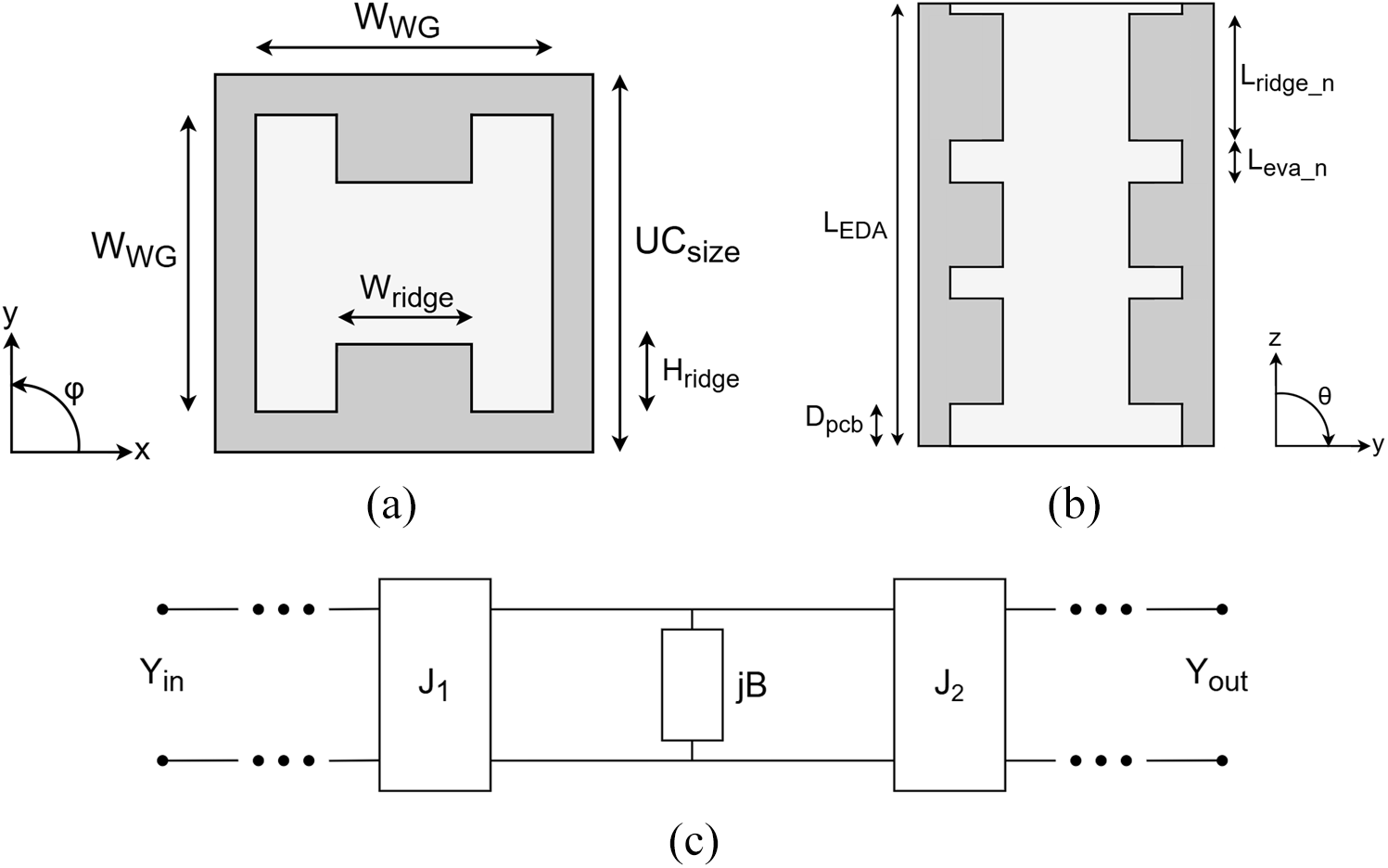
(a) Top view of the EDA, (b) cross-sectional view of the EDA, and (c) circuit representation of the EDA.

Figure 1 Long description
The top view of the EDA (image A), featuring a square waveguide with alternating ridged and non-ridged sections. The waveguide width is labeled as W subscript WG and the ridge width is labeled as W subscript ridge. The unit cell size is marked as UC subscript size and the ridge height is labeled as H subscript ridge. Axes x and y are indicated at the bottom left. The image B shows the cross-sectional view of the EDA, illustrating the alternating ridged and non-ridged sections along the length of the waveguide. The length of the EDA is labeled as L subscript EDA, with the ridge and evanescent sections marked as L subscript ridge underscore n and L subscript eva underscore n, respectively. The depth of the PCB is labeled as D subscript pcb. Axes z and y are indicated at the bottom right. The image C shows the circuit representation of the EDA, depicting an equivalent circuit model for one period of the EDA. It includes impedance inverters labeled J subscript 1 and J subscript 2 and a shunt susceptance labeled jB. The input admittance is labeled Y subscript in and the output admittance is labeled Y subscript out. Dotted lines indicate connections between these components.
Figure 1 illustrates the proposed EDA geometry. Unlike traditional waveguide antennas, which typically open gradually to facilitate the transition from guided waves to a radiated field in free space, the proposed antenna employs alternating ridged and non-ridged square waveguide sections. Proper EDA operation requires the ridged sections to function above their cutoff frequency while the non-ridged sections remain below their cutoff frequency, ensuring evanescent-mode propagation in the latter. Figure 1(c) provides an equivalent circuit model for one period of the EDA, with ridged sections modeled as shunt resonators and non-ridged evanescent sections represented as reactive impedance inverters [Reference Sanchez-Escuderos, Ruiz-Garnica, Baquero-Escudero, Soto, Boria, Toso, Angeletti and Guglielmi18, Reference Craven and Mok19]. The cutoff conditions that define these two operating regimes are quantified below for the specific dimensions of the proposed design.
The non-ridged sections of the EDA consist of square waveguide segments with lateral dimension  $W_\mathrm{WG} = 4.34$ mm (Table 1). The cutoff frequency of the dominant
 $\mathrm{TE}_{10}$ mode in an air-filled square waveguide is [Reference Hopfer16]:
 \begin{equation}
f_{c} = \frac{c}{2 W_\mathrm{WG}} ,
\end{equation}
where  $c$ is the speed of light in vacuum. Substituting
 $W_\mathrm{WG} = 4.34$ mm yields
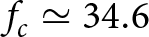 $f_{c} \simeq 34.6$ GHz, which is well above the 28 GHz operating frequency. Consequently, the electromagnetic fields in these sections decay exponentially along the waveguide axis with an attenuation constant [Reference Hopfer16]:
 \begin{equation}
\alpha = \frac{2\pi}{c} \sqrt{f_{c}^{ 2} - f^{ 2} } ,
\end{equation}
which evaluates to  $\alpha \simeq 424$ Np/m (
 $3.7$ dB/mm) at 28 GHz. The evanescent sections in Table 1 produce attenuations ranging from approximately 1 dB (
 $L_\mathrm{eva\_3}$) to 9 dB (
 $L_\mathrm{eva\_2}$), corresponding to the different inter-resonator coupling levels required by the band-pass filter synthesis. It is important to emphasize that this evanescent behavior is governed solely by the relationship
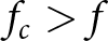 $f_{c} \gt f$ and does not require the section length to satisfy any quarter-wavelength resonance condition. The quarter-wavelength constraint applies to impedance inverters realized by propagating-mode waveguide sections, which represents a fundamentally different topology. In the presented design, the coupling strength between adjacent resonators is controlled by the product
 $\alpha L_\mathrm{eva}$, in accordance with classical evanescent-mode filter theory [Reference Craven and Mok19].
Final design parameters of the EDA antenna element expressed in mm

Table 1 Long description
Parameters and values are given in millimeters, arranged as three parameter and value pairs per row. Row 1 lists UC size 5.34, L eva 1 1.34, and L ridge 3 3.14. Row 2 lists W WG 4.34, L eva 2 2.51, and L EDA 16.4. Row 3 lists W ridge 1.33, L eva 3 0.3, and d patch 2.54. Row 4 lists H ridge 1.08, L ridge 1 3.36, and via offset 0.905. Row 5 lists D pcb 0.88, L ridge 2 4.96, and r via 0.1.
Three-dimensional view of (a) the unit cell simulation model and (b) the complete  $8 \times 8$ antenna array simulation model.

Simulated ARC obtained through unit-cell simulation.

Simulated embedded radiation pattern of the EDA along the E- and H-planes at 28 GHz obtained through simulation of a central element in an  $8 \times 8$ array. The boresight gain is 5.35 dBi.

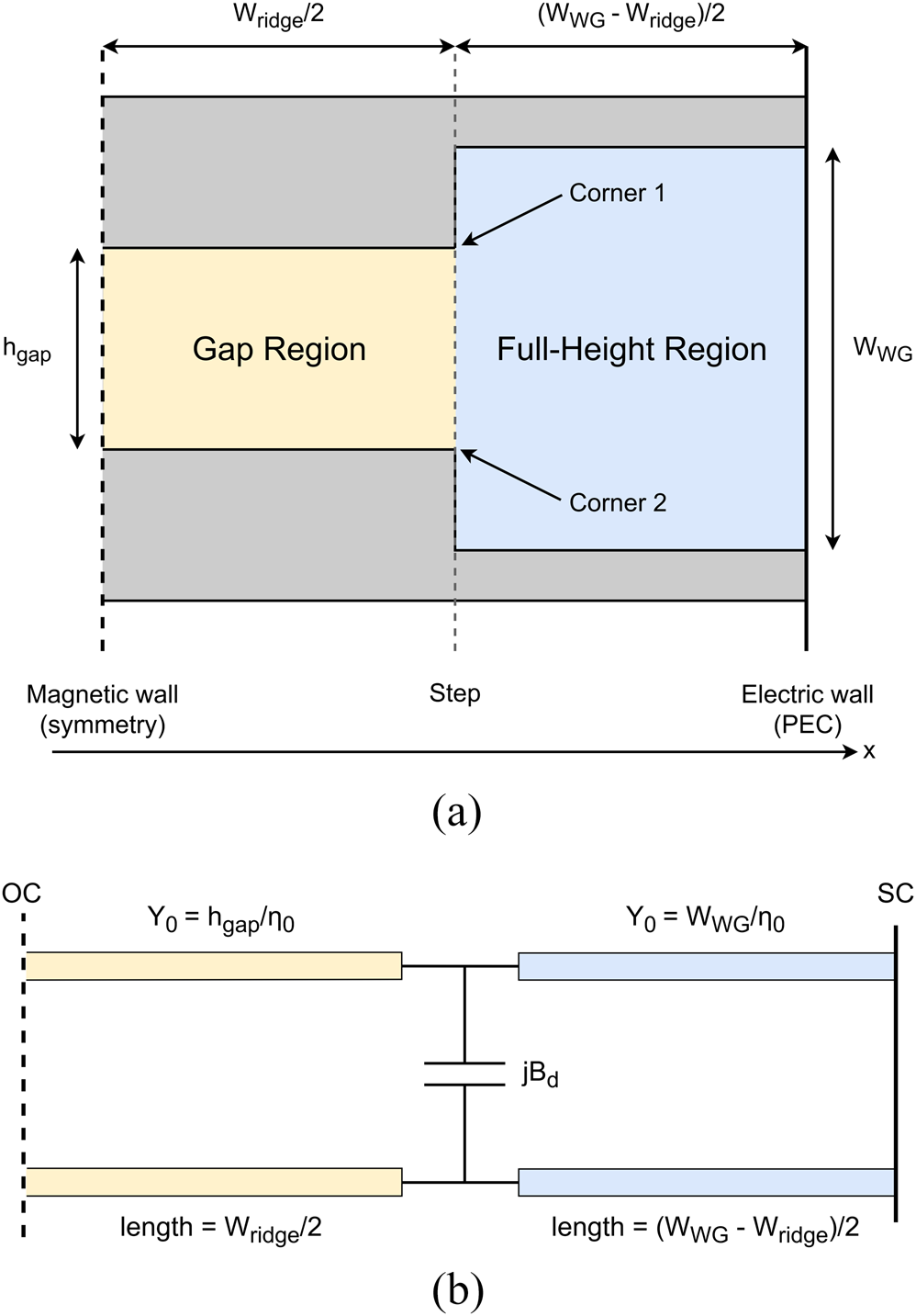
In the ridged sections, opposing metallic ridges along the E-plane walls produce a capacitive loading that substantially lowers the cutoff frequency [Reference Hopfer16, Reference Cohn20]. To quantify this effect, we apply the transverse resonance method to the half cross-section at cutoff (Figure 5), exploiting the  $\mathrm{TE}_{10}$ symmetry (
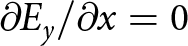 $\partial E_y/\partial x = 0$ at the waveguide center). The half-structure comprises a gap region (height
 $h_\mathrm{gap} = W_\mathrm{WG} - 2H_\mathrm{ridge}$, length
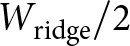 $W_\mathrm{ridge}/2$, open-circuited at the symmetry plane) and a full-height region (height
 $W_\mathrm{WG}$, length
 $(W_\mathrm{WG} - W_\mathrm{ridge})/2$, short-circuited at the PEC sidewall). Each region acts as a parallel-plate transmission line with characteristic admittance
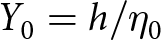 $Y_0 = h/\eta_0$ (
 $\eta_0 \simeq 377\,\Omega$). The cutoff wavenumber
 $k_c = 2\pi f_{c,\mathrm{ridged}}/c$ is the transverse propagation constant. The input admittances at the step are:
 \begin{equation}
Y_\mathrm{gap}(k_c)
= \frac{j h_\mathrm{gap}}{\eta_0}
\tan\!\left(k_c\frac{W_\mathrm{ridge}}{2}\right),
\end{equation}
 \begin{equation}
Y_\mathrm{full}(k_c)
= \frac{-j W_\mathrm{WG}}{\eta_0}
\cot\!\left(k_c\frac{W_\mathrm{WG}-W_\mathrm{ridge}}{2}\right).
\end{equation}
At the step, the abrupt change in plate separation generates fringing fields that store excess reactive energy, represented by a single shunt susceptance  $jB_d$ in the equivalent circuit (Figure 5). For a single E-plane step (one corner), the quasi-static result from Marcuvitz [Reference Marcuvitz21] gives a normalized susceptance proportional to
 $\ln[\csc(\pi h_\mathrm{gap}/(2W_\mathrm{WG}))]$. In the dual-ridged geometry, the step involves two symmetric corners (one at each ridge tip), each contributing an equal fringing susceptance. Summing both contributions yields:
 \begin{equation}
B_d(k_c)
\simeq \frac{4 W_\mathrm{WG}^{ 2} k_c}{\pi \eta_0}
\ln\!\left[\csc\!\left(
\frac{\pi h_\mathrm{gap}}{2 W_\mathrm{WG}}\right)\right].
\end{equation}
Equation (5) captures the physical mechanism: reducing  $h_\mathrm{gap}$ (i.e., deepening the ridges) increases
 $B_d$ because
 $\ln[\csc(\cdot)]$ grows as the gap narrows, thereby shifting the resonance to a lower
 $k_c$ and hence a lower cutoff frequency. The transverse resonance condition requires the total admittance at the step to vanish [Reference Hopfer16, Reference Cohn20]:
 \begin{equation}
Y_\mathrm{gap}(k_c) + Y_\mathrm{full}(k_c) + jB_d(k_c) = 0 .
\end{equation}
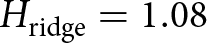
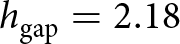
Substituting (3)–(5) and solving numerically for the dimensions in Table 1 (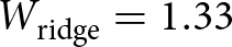 $W_\mathrm{ridge} = 1.33$ mm,
 $H_\mathrm{ridge} = 1.08$ mm,
 $h_\mathrm{gap} = 2.18$ mm) yields
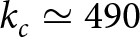 $k_c \simeq 490$ rad/m, corresponding to a ridged-section cutoff of approximately 23.4 GHz. This value is well below the 28 GHz operating frequency, confirming that the ridged sections support propagating modes throughout the operating band. It should be noted that (5) is a quasi-static result derived for infinite parallel plates and does not capture all higher-order effects present in the finite square cross-section.
The combination of propagating ridged sections (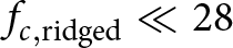 $f_{c,\mathrm{ridged}} \ll 28$ GHz) and evanescent non-ridged sections (
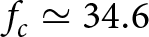 $f_{c} \simeq 34.6$ GHz
 $ \gt 28$ GHz) constitutes the hallmark of the evanescent-mode waveguide topology [Reference Polo-Lopez, Menargues, Capdevila, Toso and Garcia-Vigueras17–Reference Craven and Mok19]. In this architecture, the structure alternates abruptly between propagation and evanescence, with each ridged section forming a resonant cavity and each evanescent section acting as a reactive impedance inverter. This differs fundamentally from a stepped-ridge configuration, where all sections support propagating modes and the ridge geometry is varied progressively to achieve a broadband impedance taper. In the EDA, no gradual taper exists; instead, the filtering behavior of the evanescent-mode structure defines both the operating bandwidth and the radiation characteristics. The equivalent circuit of Figure 1(c) captures this: each ridged section is modeled as a shunt resonator with frequency-dependent susceptance
 $B_k(\omega)$, while each evanescent section is represented by an impedance inverter with coupling value
 $J_k$, following the classical filter synthesis framework of [Reference Craven and Mok19].
Transverse resonance schematic for the ridged waveguide at cutoff. (a) Half cross-section obtained by exploiting  $\mathrm{TE}_{10}$ symmetry. The outer metal walls are continuous and flush across both regions; the ridges protrude inward in the gap region only. Two step corners (at the ridge tips) generate the fringing susceptance
 $B_d$. (b) Equivalent transmission line circuit with a single shunt capacitor representing the total susceptance
 $jB_d$ at the step junction.

Figure 5 Long description
Ridged waveguide at cutoff, divided into two regions: the gap region on the left and the full-height region on the right. The gap region is labeled with height h subscript gap and length W subscript ridge over 2, while the full-height region is labeled with height W subscript WG and length W subscript WG minus W subscript ridge over 2. Two corners, labeled Corner 1 and Corner 2, are present at the junction between the regions. The magnetic wall is indicated on the left side and the electric wall, labeled PEC, is on the right side. An equivalent transmission line circuit with two sections representing the gap and full-height regions. The left section is open-circuited, labeled OC, with characteristic admittance Y subscript 0 equals h subscript gap over eta subscript 0 and length W subscript ridge over 2. The right section is short-circuited, labeled SC, with characteristic admittance Y subscript 0 equals W subscript WG over eta subscript 0 and length W subscript WG minus W subscript ridge over 2. A single shunt capacitor, labeled j B subscript d, is positioned between the two sections, representing the total susceptance at the step junction.
Multiple design approaches for evanescent-mode filters are described in the scientific literature that can be used to design the EDA [Reference Sanchez-Escuderos, Ruiz-Garnica, Baquero-Escudero, Soto, Boria, Toso, Angeletti and Guglielmi18, Reference Ozturk and N22]. These methodologies aim to determine optimal lengths for ridged and evanescent sections. Common design techniques include systematic optimization based on full-wave electromagnetic simulations and slope-parameter-based methods. In this work, a slope-parameter design approach [Reference Sanchez-Escuderos, Ruiz-Garnica, Baquero-Escudero, Soto, Boria, Toso, Angeletti and Guglielmi18] is utilized to obtain initial design values for the EDA. This step was followed by optimization through full-wave electromagnetic simulations to obtain the final design values. This slope parameter method was implemented as follows.
The first step involves calculating the inverter values  $J_k$ as:
 \begin{equation}
J_k = \sqrt{\frac{b_k\Delta b_{k+1}}{g_kg_{k+1}}},
\end{equation}
where  $\Delta$ is the fractional bandwidth,
 $b_k$ represents slope parameters of resonator sections, and
 $g_k$ are coefficients defining the desired band-pass response. Boundary parameters
 $b_0$ and
 $b_n$ are defined as
 $Y_{in}$ and
 $Y_{out}$, respectively. Intermediate slope parameters are obtained via:
 \begin{equation}
b_k = \Delta\frac{\omega_0}{2} \frac{dB_k(\omega)}{d\omega}\bigg|_{\omega = \omega_0},
\end{equation}
where  $B_k(\omega)$ is the frequency-dependent susceptance of the
 $k$-th resonator, and
 $\omega_0$ denotes the angular center frequency. These calculated values provide an initial EDA design, which can subsequently be optimized through full-wave simulations.
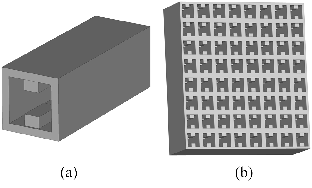
To evaluate the suitability of the EDA for active array applications, particularly those requiring beam steering, preliminary electromagnetic simulations were performed using CST Studio Suite [23]. Figure 2 depicts the unit-cell model configuration as well as the  $8 \times 8$ array configuration used for the upcoming performance analyses. The active reflection coefficient (ARC), which accounts for mutual coupling effects, is an essential parameter for assessing array antenna performance.
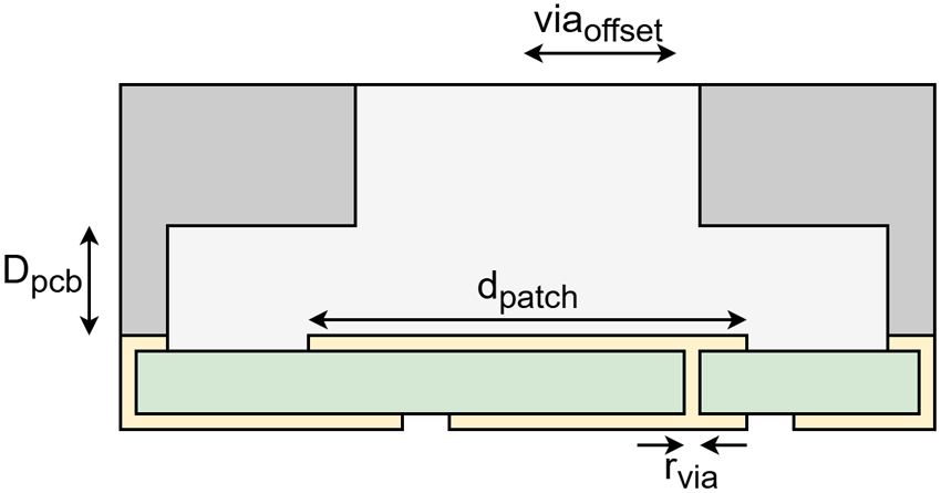
Cross-sectional view of the proposed launcher structure for the individual EDA element.

Simulated ARC of the EDA fed by the launcher structure for various scanning angles along (a) the H-plane and (b) the E-plane.

Figure 7 Long description
The contour heatmap A has an x-axis labeled, Frequency, bracket gigahertz, with ticks at 26.5, 27.0, 27.5, 28.0, 28.5, 29.0 and 29.5. The y-axis is labeled, Scan Angle theta 0, bracket degree, with ticks at 0, 10, 20, 30, 40, 50 and 60. A vertical color scale at the right is labeled, Active Reflection Coefficient, bracket decibel, with tick labels at minus 5, minus 10, minus 15 and minus 20. Two dashed contour lines are drawn and labeled, minus 10 decibel and minus 6 decibel. The minus 10 decibel contour forms a narrow band around the central low region, spanning roughly from frequency about 27.2 to 28.6 across scan angles from 0 to 60. The minus 9 decibel contour lies outside the minus 10 decibel contour and extends farther toward lower and higher frequencies. The lowest region is centered near frequency about 28.0 and extends vertically across scan angles, with the darkest area near scan angles from 0 to about 40. The contour heatmap B has an x-axis labeled, Frequency, bracket gigahertz, with ticks at 26.5, 27.0, 27.5, 28.0, 28.5, 29.0 and 29.5. The y-axis is labeled, Scan Angle theta 0, bracket degree, with ticks at 0, 10, 20, 30, 40, 50 and 60. A vertical color scale at the right is labeled, Active Reflection Coefficient, bracket decibel, with tick labels at minus 2.5, minus 5.0, minus 7.5, minus 12.5, minus 15.0 and minus 20.0. Two dashed contour lines are drawn and labeled, minus 10 decibel and minus 6 decibel. The minus 10 decibel contour encloses a central low region centered near frequency about 28.0, narrowing at low scan angles and widening toward scan angle 60. The minus 6 decibel contour lies outside the minus 10 decibel contour and reaches closer to frequencies near 27.0 on the left and near 28.8 on the right at higher scan angles.
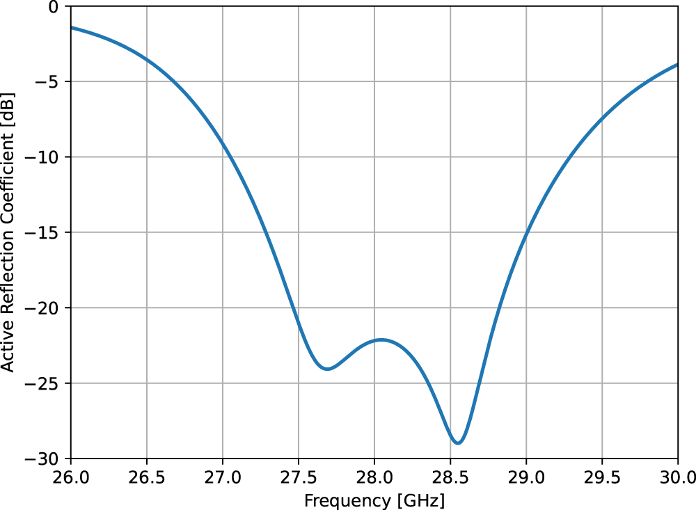
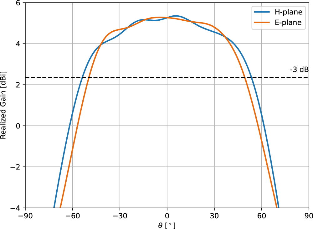
Figures 3 and 4 show the simulated ARC obtained from a unit-cell simulation and the embedded radiation pattern, respectively. It is important to note that, for this analysis, the reference impedance is the characteristic impedance of the waveguide structure rather than the conventional 50  $\Omega$. The simulated results indicate a well-matched performance around 28 GHz, achieving a bandwidth of
 $7.9\%$. While the bandwidth is limited, it can be further increased by adding additional ridged and evanescent sections, at the cost of increased complexity and size. The radiation pattern of the embedded antenna element also exhibits a broad beamwidth, which is suitable for wide-scanning array applications, with a peak gain (boresight) of 5.35 dBi. This performance is achieved while maintaining an element spacing of less than
 $0.5\lambda$, which ensures that grating lobes will not appear even when scanning to larger elevation angles. With these results and constraints in mind, the next step is to incorporate the launcher structure to be able to feed the EDA.
Launcher structure
To integrate the EDA with active arrays, a launcher structure is essential. The launcher must excite the desired waveguide mode and provide impedance transformation from the characteristic impedance of the waveguiding section to the standard 50  $\Omega$ reference impedance adopted at circuit level. Figure 6 illustrates the cross-sectional view of the proposed launcher, inspired by the design presented in [Reference Simeoni, Coman and Lager24]. This launcher consists of a circular, via-fed patch antenna mounted on a single dielectric layer (Rogers RO4350B).
The choice of a PCB-based launcher was driven by two main considerations. Firstly, the PCB integration simplifies interfacing the antenna array directly with the electronics necessary for active operation. Secondly, the selected launcher design can be straightforwardly extended to support dual polarization by introducing an additional orthogonally positioned feeding via and corresponding ridge modifications in the EDA.
The combined performance of the EDA and launcher was investigated through unit-cell simulations, and the final design parameters can be found in Table 1. Figure 7(a) and (b) illustrates the ARC for different scanning angles along the H- and E-planes, respectively. Compared to the standalone EDA, integration with the launcher structure reduces impedance bandwidth from  $7.9\%$ to
 $4.2\%$, primarily due to the limited bandwidth of the patch antenna. Although bandwidth can be improved by incorporating stacked or parasitic patches, such enhancements fall outside the scope of this study. Nevertheless, the magnitude of the ARC remains below
 $-$10 dB for scanning angles up to approximately
 $50{^\circ}$ in both planes.
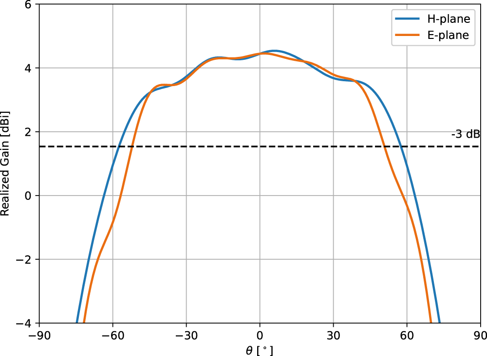
Simulated embedded radiation pattern of the EDA with the launcher structure along the E- and H-planes at 28 GHz obtained through simulation of a central element in an  $8 \times 8$ array. Boresight gain is 4.54 dBi.

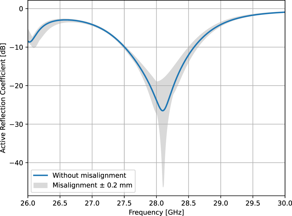
Simulated ARC range of the EDA for various misalignment values obtained through unit-cell simulation.

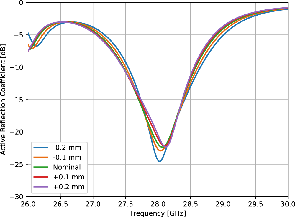
Simulated ARC range of the EDA for various misalignment values obtained through unit-cell simulation.

Simulated ARC range of the EDA for various misalignment values obtained through unit-cell simulation.

Figure 11 Long description
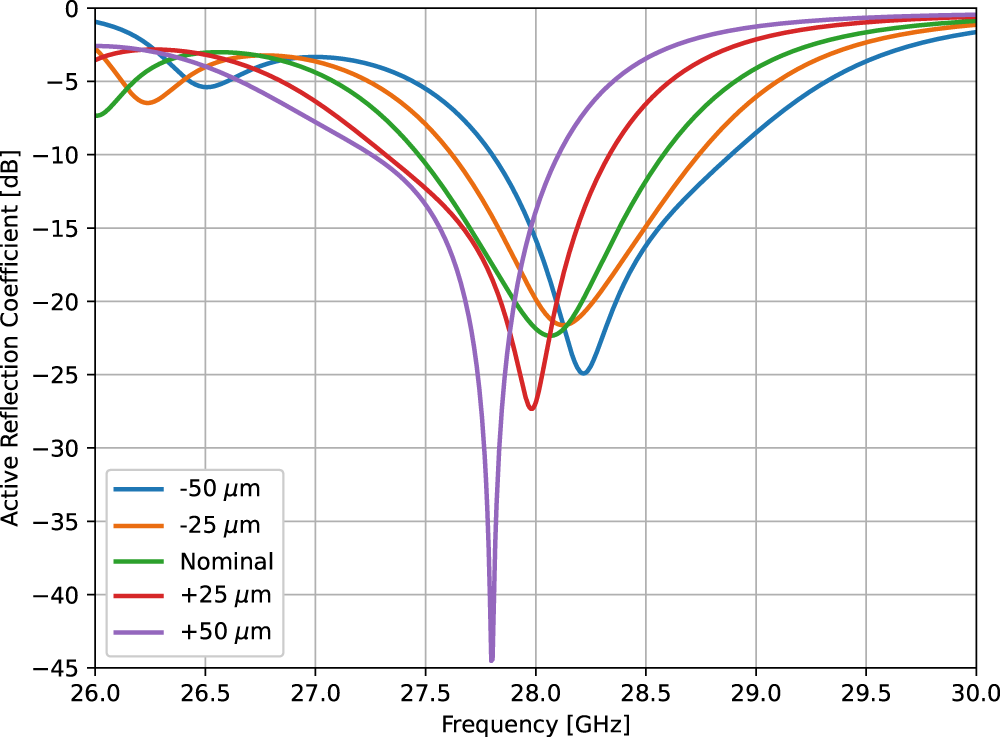
Active Reflection Coefficient [dB]. Frequency [GHz]. The x-axis ranges from 26.0 to 30.0 with ticks at 26.0, 26.5, 27.0, 27.5, 28.0, 28.5, 29.0, 29.5 and 30.0. The y-axis ranges from 0 to minus 45 with ticks at 0, minus 5, minus 10, minus 15, minus 20, minus 25, minus 30, minus 35, minus 40 and minus 45. A legend lists five series: minus 50 micro-meter, minus 25 micro-meter, Nominal, plus 25 micro-meter, plus 50 micro-meter. Minus 50 micro-meter curve: about minus 1 at 26.0, about minus 5 at 26.5, about minus 3 at 27.0, about minus 5 at 27.5, about minus 15 at 28.0, minimum about minus 25 near 28.2, about minus 16 at 28.5, about minus 9 at 29.0, about minus 4 at 29.5, about minus 2 at 30.0. Minus 25 micro-meter curve: about minus 3 at 26.0, about minus 4 at 26.5, about minus 3 at 27.0, about minus 8 at 27.5, about minus 20 at 28.0, minimum about minus 22 near 28.1, about minus 15 at 28.5, about minus 6 at 29.0, about minus 3 at 29.5, about minus 2 at 30.0. Nominal curve: about minus 7 at 26.0, about minus 3 at 26.5, about minus 4 at 27.0, about minus 11 at 27.5, about minus 22 at 28.0, minimum about minus 22 near 28.1, about minus 12 at 28.5, about minus 4 at 29.0, about minus 2 at 29.5, about minus 1 at 30.0. Plus 25 micro-meter curve: about minus 3 at 26.0, about minus 4 at 26.5, about minus 6 at 27.0, about minus 12 at 27.5, about minus 27 near 28.0, about minus 6 at 28.5, about minus 2 at 29.0, about minus 1 at 29.5, about minus 1 at 30.0. Plus 50 micro-meter curve: about minus 2 at 26.0, about minus 5 at 26.5, about minus 8 at 27.0, about minus 13 at 27.5, minimum about minus 45 near 27.8, about minus 4 at 28.5, about minus 1 at 29.0, about minus 1 at 29.5, about minus 1 at 30.0.
Figure 8 presents the simulated ERP of the central element within an  $8 \times 8$ array, including the launcher structure. The launcher-integrated EDA exhibits an half-power beamwidth (HPBW) of
 $115.2{^\circ}$ along the H-plane and
 $103.6{^\circ}$ along the E-plane, thus confirming the suitability of the proposed design for wide-angle scanning array applications. The boresight gain with the launcher is about 0.8 dB lower than without the launcher, which can be attributed to a wider beamwidth as well as losses introduced by the launcher structure.
Exploded view of the  $8 \times 8$ EDA array demonstrator assembly.

Figure 12 Long description
A vertically separated stack of parts is shown in an exploded assembly order. At the top is a square top plate with a recessed square field of repeated square openings and four corner posts that align with four long threaded fasteners running downward through the stack. Directly below is a second square plate with a similar recessed field of repeated openings, aligned to the same four corner fasteners. Below that are two thicker square spacer like plates, each with a large central square cutout and a perimeter frame, aligned on the same corner fasteners. Beneath the spacer plates are three flat rectangular boards shown as separate layers, each with corner mounting holes aligned to the fasteners; the upper board has a dense rectangular array of small square pads or openings, the middle board shows a larger square grid pattern and the lower board shows a field of small circular holes arranged in rows. At the bottom is a rectangular pin grid connector layer with many evenly spaced cylindrical pins projecting downward in a rectangular array, aligned under the lower board. The diagram presents the mechanical stack up and alignment of the fasteners, plates, boards and the pin grid connector as a single assembly.
Photograph of the fully assembled  $8 \times 8$ EDA array prototype used for the experimental measurements.

Photographs of the measurement setups used to validate the performance of the  $8 \times 8$ EDA array prototype for (a) the embedded radiation pattern measurements in a spherical anechoic chamber and (b) the efficiency measurements in a reverberation chamber.

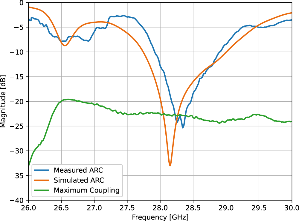
Measured and simulated ARC of a central element in the  $8 \times 8$ EDA array prototype for boresight scanning. The maximum coupling level between the considered array element and the adjacent ones is also shown.

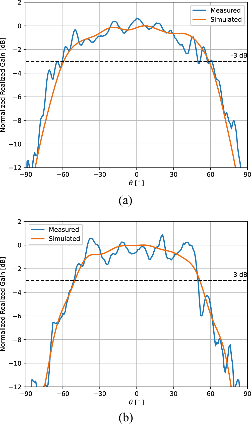
Measured embedded radiation patterns of a central element in the  $8 \times 8$ EDA array prototype at 28 GHz compared with simulation results along (a) H-plane and (b) E-plane. Broadside gain measured at 3.45 dBi and simulated at 4.23 dBi.

Measured scanning performance of the  $8 \times 8$ EDA array prototype at 28 GHz compared with the simulation results for scanning angles along the (a) H-plane and (b) E-plane. The red, dashed line shows the scan loss as predicted by the cosine law. Broadside gain estimated from measurements at 21.41 dBi and simulated at 21.99 dBi.

Figure 17 Long description
A line graph comparing measured and simulated normalized realized gain versus theta for different scan angles along the H-plane. The x-axis is labeled theta, degrees, ranging from minus 90 to 90. The y-axis is labeled Normalized Realized Gain, decibel, ranging from minus 20 to 5. Multiple curves represent different beams, with peaks near 0 degrees. A dashed line at minus 3 decibel indicates the beamwidth region where curves stay above this threshold. The measured curves (blue) and simulated curves (orange) show agreement in peak locations but vary in amplitude across angles. The image B showing a line graph comparing measured and simulated normalized realized gain versus theta for different scan angles along the E-plane. The x-axis is labeled theta, degrees, ranging from minus 90 to 90. The y-axis is labeled Normalized Realized Gain, decibel, ranging from minus 20 to 5. Multiple curves represent different beams, with peaks near 0 degrees. A dashed line at minus 3 decibel indicates the beamwidth region where curves stay above this threshold. The measured curves (blue) and simulated curves (orange) show agreement in peak locations but vary in amplitude across angles. Both panels share the same axis labels and legend, with the main takeaway being the comparison of measured versus simulated performance across different scan angles and planes.
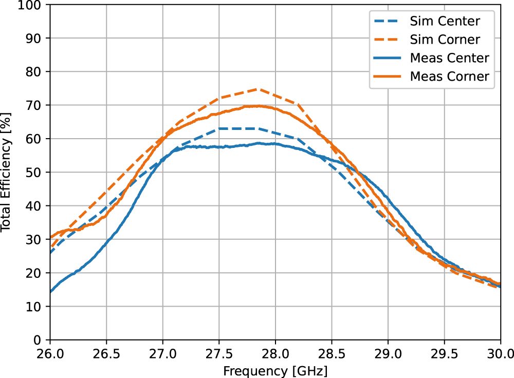
Measured total efficiency of the  $8 \times 8$ EDA array prototype for a center and a corner element compared with simulation results.

 $8 \times 8$ EDA array design

In the previous section, the EDA performance was evaluated through unit-cell simulations, highlighting its key electromagnetic characteristics. In this section, we extend the evaluation to a complete  $8 \times 8$ EDA array prototype through comprehensive full-wave simulations and experimental measurements. The prototype comprises two primary components: a metallic EDA structure and a PCB featuring the integrated launcher structure. An exploded view of the array assembly is presented in Figure 12.
The EDA array demonstrator was fabricated using aluminum via computer numerical control (CNC) machining. Two main adjustments were necessary to facilitate this manufacturing approach. Firstly, inner corners within the EDA structure were rounded with a radius of 0.25 mm to account for the finite radius of the CNC milling tip. This rounding slightly reduces the effective cross-sectional dimensions of the waveguide, resulting in a minor increase in its cutoff frequency. To compensate for this effect, the height of the ridges was marginally increased. Secondly, due to alternating ridged and non-ridged waveguide sections, realizing the entire  $8 \times 8$ array from a single aluminum block is impractical. Consequently, the array was subdivided longitudinally into multiple layers. Each layer was individually fabricated and subsequently assembled, offering a practical yet precise manufacturing solution using inexpensive conventional CNC techniques.
The layered structure inherently introduces the possibility of misalignment between adjacent layers along the  $x$- and
 $y$-directions. Figure 9 illustrates the simulated impact of such misalignment. Here, the grey region presents the envelope of all misalignment results between
 $\pm$0.2 mm. This reveals that the resonance frequency is barely impacted for misalignment on this order; only the matching is deteriorated if the layer alignment is not properly controlled. It is still necessary to carefully align the layers to achieve optimal performance. To facilitate the accurate assembly of the layers, an extended frame was incorporated around the array perimeter to accommodate assembly bolts. These bolts are recessed such that their heads remain flush with the top surface of the array, minimizing any potential adverse electromagnetic effects. The same bolts serve dual purposes, providing mechanical stability and keeping the PCB-based launcher in contact with the metal array structure.
To further understand the implications of manufacturing tolerances on the proposed design, a parameter study was performed specifically on the metal array design. Figures 10 and 11 show the ARC in unit-cell simulations for various values of  $W_\mathrm{ridge}$ and
 $H_\mathrm{ridge}$, respectively. The array response is consistent for tolerances on
 $W_\mathrm{ridge}$; however, this is not the case for
 $H_\mathrm{ridge}$, where even tolerances on the order of 50 µm can produce a noticeable frequency shift. It is therefore important that the height of the ridge is well controlled, which is achievable with the proposed CNC manufacturing methodology.
An  $8 \times 8$ EDA array prototype was fabricated based on the considerations outlined above, with a representative photograph shown in Figure 13. The prototype was evaluated by comparing full-wave simulation-based predictions against measured data obtained from experimental characterization.
Firstly, the ARC of a central array element was measured using a Keysight P5028A vector network analyzer (VNA) [25]. The ARC was determined by measuring the coupling from the element under test to all other elements and then combining these measurements in post-processing. During these measurements, all other elements were terminated with 50  $\Omega$ loads. The simulated and measured performance is illustrated in Figure 15. A slight frequency shift between simulations and measurements can be observed, likely attributable to manufacturing tolerances and minor misalignments during assembly. Despite this shift, the overall measured ARC closely matches the simulated one, confirming the robustness of the electromagnetic characteristics of the developed antenna solution. Furthermore, the maximum inter-element coupling remains below approximately
 $-$20 dB across the entire operating frequency band.
Next, the embedded element radiation patterns were experimentally evaluated in a spherical anechoic chamber, as depicted in Figure 14(a). The array was mounted centrally within the chamber on a custom-designed 3D-printed fixture, and a rotating horn antenna probe captured the radiated power levels at multiple elevation angles  $\theta$ along the E- and H-planes. The horn antenna probe can be rotated, thus allowing for comprehensive co- and cross-polarization characterization.
The measured and simulated embedded radiation patterns for a central array element at 28 GHz are compared in Figure 16(a) (H-plane) and Figure 16(b) (E-plane). The measurements align closely with numerical simulations, aside from minor ripples introduced by spurious reflections occurring in the anechoic chamber. To mitigate these measurement artifacts, normalization was performed against the average main beam power rather than the peak power level. The agreement in terms of HPBW further supports this alignment, with measured values of  $121{^\circ}$ (H-plane) and
 $102{^\circ}$ (E-plane) closely matching the simulated values of
 $119{^\circ}$ and
 $102{^\circ}$, respectively, showing a deviation of at most
 $2{^\circ}$. From these measurements, the gain of a central element was estimated at 3.45 dBi using a comparative method. The same element achieved a gain of 4.23 dBi in simulation. Since the tolerance of the anechoic chamber is estimated at 1.5 dB, this falls well within the measurement tolerance and is considered a good match; any residual discrepancies can be attributed to manufacturing tolerances as well as additional conductor losses.
Additionally, the array scanning characteristics have been evaluated numerically by combining the measured embedded radiation patterns for individual antenna elements. Figure 17 illustrates a strong agreement between the simulated and reconstructed measured beam-scanning properties at 28 GHz. A 3-dB scanning range of approximately  $116{^\circ}$ along the H-plane (
 $-60{^\circ}$ to
 $56{^\circ}$) and
 $96{^\circ}$ along the E-plane (
 $-47{^\circ}$ to
 $49{^\circ}$) was experimentally demonstrated. These results closely match the simulated scanning ranges of
 $112{^\circ}$ (H-plane) and
 $98{^\circ}$ (E-plane), with discrepancies within
 $4{^\circ}$. Finally, based on the measured performance of the individual antenna elements, the broadside array gain was calculated to be 21.41 dBi, which agrees well with the 21.99 dBi value predicted by numerical electromagnetic simulations.
Lastly, the total efficiency of the array elements was evaluated using the reverberation chamber setup shown in Figure 14(b). During these measurements, the non-active antenna elements were terminated with 50- $\Omega$ loads. Figure 18 compares the simulated and measured characteristics for both central and corner elements of the array, indicating excellent agreement with deviations below 5%. Higher efficiencies observed for corner elements compared to central elements highlight the influence of reduced inter-element coupling. Note that the actual efficiency values are likely slightly higher than presented due to additional connector losses included in the reported measurements.
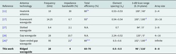
Table 2 summarizes the measured array characteristics and compares them against state-of-the-art metal-based antenna arrays recently reported in the literature. This comparison highlights the competitive performance of the proposed EDA design. It should, however, be emphasized that the efficiency values cited from these references were obtained under conditions that are considerably more favorable. Specifically, in [Reference Banerjee, Sharma, Chieh and Farkouh11], the total efficiency is presented based solely on simulation results for a  $4 \times 2$ sub-array, which naturally experiences reduced coupling losses compared to the full-scale array implementation assessed in our work. Additionally, it is noteworthy that our simulations explicitly incorporate realistic factors, such as surface roughness and connector losses, to provide the most accurate and practically relevant efficiency estimate.
Similarly, the efficiency reported in [Reference Polo-Lopez, Menargues, Capdevila, Toso and Garcia-Vigueras17] is evaluated for a single, isolated antenna element, thereby neglecting coupling losses. As discussed earlier, coupling losses significantly contribute to the overall loss budget, making the isolated-element efficiency inherently higher and less representative of practical array scenarios. Furthermore, [Reference Zhang, Vilenskiy and Ivashina26] provides only radiation efficiency obtained through simulation, inherently omitting critical matching and coupling losses, which results in artificially elevated efficiency values.
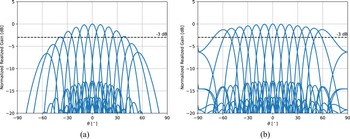
Finally, we wish to underscore once again the significance of performing comprehensive finite-array simulations. Figure 19 illustrates the scanning performance derived from the unit-cell radiation pattern simulations. It clearly demonstrates significant discrepancies between these unit-cell simulation results and the previously discussed measurement and finite-array simulation outcomes. This discrepancy strongly indicates that unit-cell-based simulations alone cannot reliably predict the true radiation patterns and performance characteristics of practical, full-scale antenna arrays.
Thermal characterization
In the preceding sections, the performance of the proposed EDA array has been analyzed from an electromagnetic perspective. However, one of the primary advantages of a metal-based antenna design lies in its enhanced thermal characteristics, which are especially critical for active array architectures. This section presents a comprehensive thermal analysis of the EDA array, including both simulation and experimental validation. The thermal performance is also benchmarked against an equivalent patch antenna array structure.
Performance comparison of state-of-the-art metal-based antenna arrays available in the scientific literature

Table 2 Long description
Rows compare six references by antenna technology, frequency in gigahertz, impedance bandwidth in percent, total efficiency in percent, element spacing in free space wavelength, 3 decibel scan range in E plane and H plane, and array size. Heat Sink Antenna, reference 11, lists 10 gigahertz, 30 percent bandwidth, total efficiency 80 marked S and star, spacing 0.53 by 0.53, scan range 100 degrees E plane and 60 degrees H plane, and array size 2 by 4. Evanescent Waveguide, reference 17, lists 14.25 gigahertz, 6.7 percent bandwidth, total efficiency 93 marked star, spacing 0.54 by 0.54, scan range 100 degrees E plane and 100 degrees H plane marked S, and array size 16 by 16. Slotted Waveguide, reference 27, lists 9.4 gigahertz, 2.1 percent bandwidth, total efficiency shown as not available, spacing 0.7, scan range 84 degrees E plane and 0 degrees H plane, and array size 1 by 8. Gap Waveguide, reference 28, lists 28 gigahertz, 10.7 percent bandwidth, total efficiency shown as not available, spacing 2.24 by 0.52, scan range 120 degrees E plane and 0 degrees H plane, and array size 4 by 16. Open Ended Gap Waveguide, reference 26 marked star, lists 95 gigahertz, impedance bandwidth 21 marked S, total efficiency 89 marked S and double asterisk, spacing 0.5 by 0.6, scan range 102 degrees E plane and 100 degrees H plane marked S, and array size listed as Infinite. This work, Ridged Waveguide, lists 28 gigahertz, 4 percent bandwidth, total efficiency 60 to 70, spacing 0.5 by 0.5, scan range 96 degrees E plane and 116 degrees H plane, and array size 8 by 8.
S Only simulated result available.
* Achieved using a single standalone element or a smaller subset of the array.
** Radiation efficiency.
Simulated scanning performance of an  $8 \times 8$ array at 28 GHz constructed from the unit cell radiation pattern along the (a) H-plane and (b) E-plane.

Figure 19 Long description
A line graph with multiple overlaid beam pattern curves. The x-axis label is theta, degrees, with tick labels at minus 90, minus 60, minus 30, 0, 30, 60, 90. The y-axis label is Normalized Realized Gain, decibel, with tick labels at 5, 0, minus 5, minus 10, minus 15, minus 20. A dashed horizontal line is labeled minus 3 decibel. The overlaid curves have main lobes centered at different theta values between about minus 60 degrees and plus 60 degrees. The highest parts of the main lobes reach near 0 decibel. Many sidelobe traces and oscillations appear below about minus 12 decibel, with dense overlapping curves between about minus 40 degrees and plus 40 degrees. The image B showing a line graph with multiple overlaid beam pattern curves. The x-axis label is theta, degrees, with tick labels at minus 90, minus 60, minus 30, 0, 30, 60, 90. The y-axis label is Normalized Realized Gain, decibel, with tick labels at 5, 0, minus 5, minus 10, minus 15, minus 20. A dashed horizontal line is labeled minus 3 decibel. The overlaid curves have main lobes centered at different theta values spanning roughly minus 60 degrees to plus 60 degrees. The tops of the main lobes reach near 0 decibel. Numerous sidelobe traces and oscillations appear below about minus 12 decibel, with dense overlapping curves concentrated between about minus 40 degrees and plus 40 degrees and additional curved traces extending toward minus 90 degrees and plus 90 degrees.
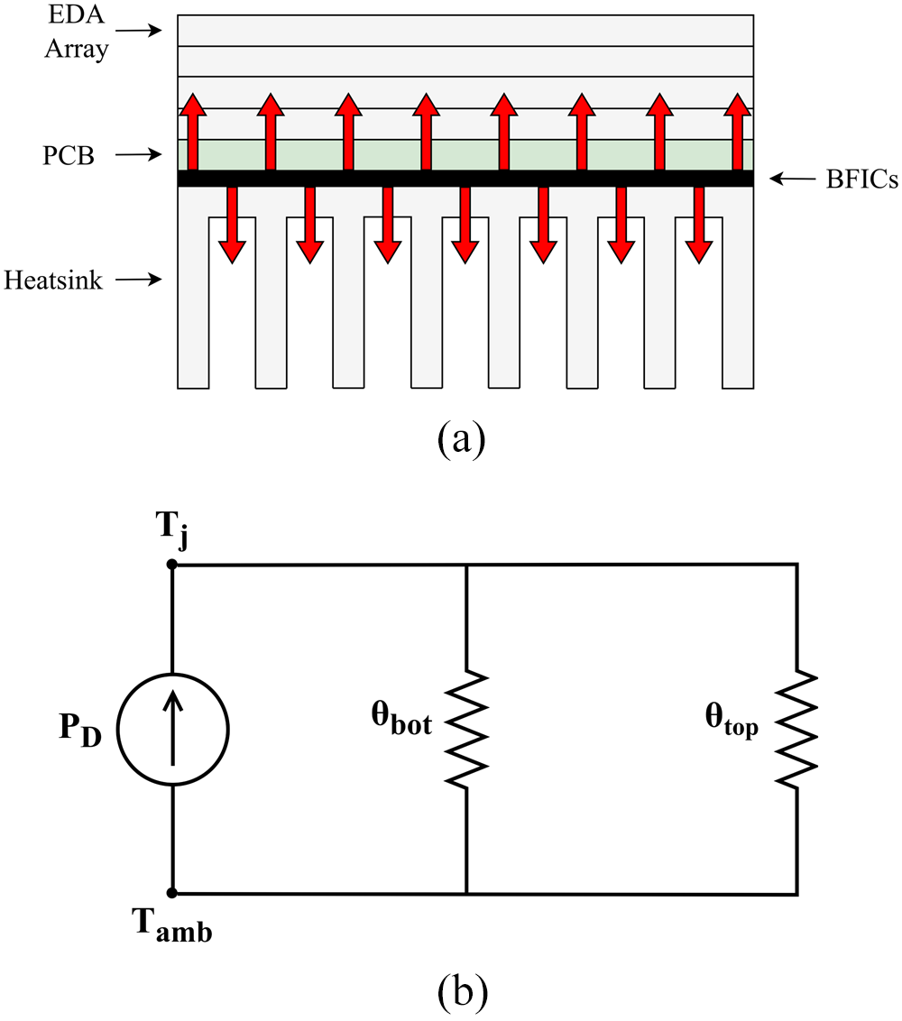
To assess the thermal behavior of the EDA array, it is essential to understand the physical mechanisms governing heat dissipation in an active antenna array system. Active arrays typically rely on BFICs mounted on a PCB, which facilitate electronic beam steering and signal processing. These BFICs inherently generate substantial heat during operation. Efficient heat removal is crucial to maintaining safe junction temperatures and ensuring long-term reliability. The generated heat can dissipate through two primary paths: downward through the PCB to a dedicated heat sink, and upward through the antenna array itself through a dedicated via network. Figure 20(a) illustrates this dual-path thermal behavior.
A widely adopted model to describe this phenomenon is the two-resistor thermal model [29], which characterizes the thermal resistances of the top and bottom conduction paths as  $\theta_\mathrm{top}$ and
 $\theta_\mathrm{bot}$, respectively. These resistances quantify the effectiveness of each path in conducting heat, with lower values indicating superior thermal conduction. The equivalent thermal circuit is shown in Figure 20(b), where thermal resistances are modeled as electrical resistors, temperatures as voltages, and the heat source (with power dissipation
 $P_D$) as a current source. Following Ohm’s law, the junction temperature
 $T_J$ can be expressed as:
 \begin{equation}
T_J = T_\mathrm{amb} + P_D \frac{\theta_\mathrm{bot} \theta_\mathrm{top}}{\theta_\mathrm{bot} + \theta_\mathrm{top}},
\end{equation}
where  $T_\mathrm{amb}$ denotes the ambient temperature.
To isolate the thermal contribution of the antenna path, both the simulations and the measurements presented in this section are deliberately configured without a bottom heatsink. In the equivalent thermal circuit of Figure 20(b), this corresponds to  $\theta_\mathrm{bot} \rightarrow \infty$ (i.e., an open circuit in the thermal network). Under this condition, (9) reduces to:
 \begin{equation}
T_J = T_\mathrm{amb} + P_D \theta_\mathrm{top} .
\end{equation}
Equation (10) shows that, in the absence of the bottom-side thermal path, the temperature rise above ambient is governed entirely by  $\theta_\mathrm{top}$. This open-circuit configuration provides a direct and unambiguous characterization of the thermal resistance of the antenna structure, without requiring any assumption regarding
 $\theta_\mathrm{bot}$. The thermal resistance
 $\theta_\mathrm{top}$ therefore serves as a suitable figure of merit for evaluating the thermal performance of the antenna.
For the antenna path to provide a meaningful contribution to heat dissipation in an operational system,  $\theta_\mathrm{top}$ must be comparable to
 $\theta_\mathrm{bot}$. In densely integrated mmWave arrays, the bottom-side thermal path is often severely constrained by the limited PCB area and dense BFIC packaging, which can result in
 $\theta_\mathrm{bot}$ values that are significantly higher than those encountered in conventional lower-frequency systems. Under such conditions, a low
 $\theta_\mathrm{top}$ becomes critically important, as the antenna structure constitutes the primary parallel thermal conduction channel available for reducing the effective thermal resistance and, consequently, the junction temperature.
(a) Schematic view of the thermal paths and (b) equivalent circuit describing the thermal behavior of the  $8 \times 8$ EDA array prototype.

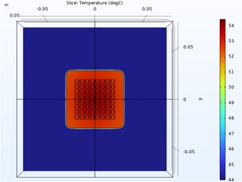
Simulated temperature of the EDA array using COMSOL Multiphysics.

Figure 21 Long description
Slice Temperature [degC]. A square heatmap is shown inside a 3D-style frame. A vertical and a horizontal line cross at the center of the square. The x-axis is labeled m, with tick labels at minus 0.05, 0 and 0.05. The y-axis is labeled m, with tick labels at minus 0.05, 0 and 0.05. A vertical color scale at the right is labeled from 44 to 54 in steps of 1. The main square field is mostly at the lowest end of the scale. A rounded-corner square region centered in the plot is at the highest end of the scale. Inside this central region is a regular grid of small square marks. The central crosshair intersection aligns with the center of the rounded-corner square region.
Photograph of the thermal measurement setup used to measure the thermal resistance of the EDA array prototype.

Measured steady-state temperatures of the EDA array for four separate measurements using the described measurement setup.

Figure 23 Long description
Four thermograms labeled (a), (b), (c) and (d) show the steady-state temperature distribution of an EDA array. Each image features a color scale on the right, ranging from approximately 26.8 degrees Celsius to 52.2 degrees Celsius. The central area of the array consistently shows higher temperatures, peaking around 51.9 degrees Celsius, while the borders are cooler. The images indicate a consistent spatial pattern across all panels, with the hottest region at the center and a gradual decrease towards the edges. The temperature readout at the top of each panel confirms the maximum temperature, with slight variations between panels. The consistent pattern suggests uniform heating across trials.
To quantify  $\theta_\mathrm{top}$, thermal simulations were performed using COMSOL Multiphysics [30], following the methodology outlined in [Reference Baldry, Timchenko and Menictas31]. Consistent with the open-circuit condition described above, only the metallic portion of the EDA array was included in the model, with no bottom heatsink present. Previous studies have shown that an optimized network of thermal vias can render the thermal resistance of the circuit board negligible [Reference Shen, Wang, Blaabjerg, Zhao and Long32], ensuring efficient thermal energy transfer from the bottom of the PCB to the antenna structure. The simulation environment included a heat source positioned at the bottom of the array, mimicking the heat generation of BFICs with a heat flow rate equivalent to
 $P_D$, as well as a laminar airflow model incorporating natural convection and gravity effects. The thermal resistance was then calculated from (10) as:
 \begin{equation}
\theta_\mathrm{top} = \frac{\Delta T}{P_D},
\end{equation}
where  $\Delta T = T_J - T_\mathrm{amb}$ represents the temperature difference between the array and the ambient temperature.
Figure 21 presents the simulated steady-state temperature distribution of the EDA array. The maximum temperature was found to be 53.6 ${^\circ}\text{C}$. Substituting into (11) yields a thermal resistance of
 $11.67~\text{K/W}$. For comparison, the same simulation procedure was applied to a commercial patch antenna array described in [Reference Ogurtsov, Song and Caratelli33], resulting in a thermal resistance of
 $123.3~\text{K/W}$. This highlights the superior thermal performance of the proposed EDA array, which achieves more than an order-of-magnitude improvement.
To validate the simulation results experimentally, a thermal measurement setup was developed. Figure 22 shows a photograph of the setup, which consists of two primary components. The first component is the EDA array prototype, thermally coupled to a resistive heating element and mounted on a 3D-printed fixture. The heating element is, in turn, connected to a controllable power source and generates heat by converting electrical power, effectively mimicking the physical mechanism modeled in the numerical thermal simulation. The heating element is a purely resistive load that converts all supplied electrical power directly into heat (Joule heating), so the generated thermal power equals the electrical input power ( $P_D = V \times I = 2.88$ W). The second component is an overhead thermal camera mounted on a fixed platform, which captures the surface temperature distribution of the array, allowing for the evaluation of the relevant thermal resistance. As in the simulation, no bottom heatsink is present, so that the open-circuit condition
 $\theta_\mathrm{bot} \rightarrow \infty$ holds and the measured temperature rise is governed entirely by (10).
Thermal measurements were performed by operating the heating element at a power of  $2.88~\text{W}$. Prior to each measurement, the array was cooled to ambient temperature to ensure repeatability. Figure 23 displays the thermal camera images from four separate measurement iterations. The maximum temperature across the measurements remained highly consistent, exhibiting a variation of no more than 0.3
 ${^\circ}\text{C}$. Using the measured
 $\Delta T$ and known power dissipation level within the heating element, the thermal resistance of the EDA array structure was calculated using (11), yielding a value of
 $11.11~\text{K/W}$. This result closely matches the simulated value (within
 $0.55~\text{K/W}$), thereby validating the design methodology and confirming the superior thermal performance of the EDA array. The measured value is comparable to typical junction-to-board thermal resistances reported in the mmWave active array literature [Reference Aslan, Puskely, Janssen, Geurts, Roederer and Yarovoy9], further confirming that the antenna path provides a substantial parallel thermal conduction channel in practical array configurations.
Conclusion
This paper has introduced and experimentally validated a novel thermally enhanced EDA array tailored for mmWave wireless communications. The proposed design leverages a fully metallic, layer-based construction to enable improved heat dissipation, wide-angle scanning capabilities, and integration with planar electronics via a PCB-based launcher structure. This architecture addresses one of the critical bottlenecks in high-frequency active antenna systems: excessive temperature rise due to densely integrated, low-efficiency beamforming electronics.
An  $8 \times 8$ EDA array prototype was rigorously evaluated through full-wave simulations and validated through comprehensive experimental characterization, including ARCs, embedded radiation patterns, beam-scanning characteristics, and thermal resistance measurements. Electromagnetic performance assessments revealed a wide scanning range of
 $116{^\circ}$ and
 $96{^\circ}$ along the H- and E-planes, respectively, with excellent agreement between simulated and measured results. The array demonstrated robust radiation properties even in the presence of manufacturing-induced deviations and bandwidth limitations imposed by the launcher structure.
From a thermal standpoint, the EDA array showcased a remarkable improvement over conventional patch antenna arrays. Thermal simulations and measurements confirmed a thermal resistance of  $11.11~\text{K/W}$, more than an order of magnitude lower than that of a standard PCB-based patch array (measured at
 $123.3~\text{K/W}$). These findings validate the EDA array as a highly promising solution for thermally constrained mmWave active array systems, offering a viable pathway toward practical, scalable, and thermally efficient implementations.
Despite the promising results achieved in this study, several avenues remain open for further exploration:
• Active array integration: The current work has focused on passive measurements and thermal characterization. A logical next step is to integrate BFICs with the proposed EDA array to evaluate system-level performance in an active environment, including thermal behavior under realistic operating conditions and beam-steering accuracy under dynamic loading.
• Launcher optimization: While the PCB-based patch launcher simplifies integration with planar electronics, it imposes limitations on the achievable impedance bandwidth. Future research may explore advanced launcher designs such as stacked or aperture-coupled patches, wideband ridge-to-microstrip transitions, or additive manufacturing-based feeds to extend the array’s operational bandwidth.
• Dual-polarization implementation: Although the current EDA design supports only single polarization, the structure is inherently extendable to dual polarization. Implementing and characterizing a dual-polarized version would broaden the array’s applicability to multiple-input multiple-output (MIMO) systems and polarization-diverse mmWave architectures.
• Thermal management enhancements: Further thermal performance gains could be achieved through advanced cooling strategies such as topology-optimized heat sinks. Additionally, co-design approaches that simultaneously consider RF and thermal constraints during the array design process may yield superior trade-offs.
• Large-scale arrays and system-level evaluations: Extending the EDA concept to larger array sizes and evaluating its impact on full 5G/6G transceiver systems, including link-level performance, electromagnetic interference, and robustness under varying environmental conditions, constitutes a critical direction for real-world deployment.
• Manufacturing tolerances and reliability: Although the proposed layered CNC-manufacturing approach is efficient and reproducible, further studies are needed to assess long-term mechanical reliability, tolerance to thermal cycling, and sensitivity to tolerances or manufacturing variations in large-scale production.
Through development along these lines, the presented EDA array design approach may evolve into an effective technology for next-generation mmWave networks, enabling high-gain, wide-angle scanning arrays that are not only electrically efficient but also thermally resilient.
Monte Carlo analysis of phase and amplitude errors for the 8 $\times$8 EDA array at 28 GHz: (a)
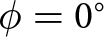 $\phi = 0{^\circ}$ cut plane; (b)
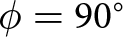 $\phi = 90{^\circ}$ cut plane. The analysis assumes a phase-error standard deviation of
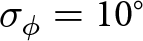 $\sigma_\phi = 10{^\circ}$, an amplitude-error standard deviation of
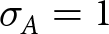 $\sigma_A = 1$ dB, and
 $N = 500$ Monte Carlo iterations.

Figure A1 Long description
Five line graphs titled, Scan equals minus 60 degrees, Scan equals minus 30 degrees, Scan equals plus 0 degrees, Scan equals plus 30 degrees and Scan equals plus 60 degrees. Each graph has the y-axis labeled, Normalized Array Factor in decibel, ranging from minus 40 to 0 with ticks every 5. Each graph has the x-axis labeled, theta in degrees, ranging from minus 90 to 90 with ticks every 30. A legend below the row lists four series: Ideal, Phase only mean, Amplitude only mean and Combined mean. In each graph, the curves form one dominant peak near the scan angle and multiple sidelobe ripples with several deep nulls that reach close to minus 40 decibel. The main peak rises to near 0 decibel. The sidelobe region shows repeated oscillations across the theta range. The image B showing five line graphs titled, Scan equals minus 50 degrees, Scan equals minus 30 degrees, Scan equals plus 0 degrees, Scan equals plus 30 degrees and Scan equals plus 50 degrees. Each graph has the y-axis labeled, Normalized Array Factor in decibel, ranging from minus 40 to 0 with ticks every 5. Each graph has the x-axis labeled, theta in degrees, ranging from minus 90 to 90 with ticks every 30. A legend below the row lists four series: Ideal, Phase only mean, Amplitude only mean and Combined mean. In each graph, the curves show a dominant peak near the scan angle and a sequence of sidelobe ripples with multiple deep nulls that drop close to minus 40 decibel. The main peak rises to near 0 decibel. The oscillations extend across most of the theta range, with the deepest dips occurring at several angles on both sides of the main peak.
Acknowledgements
This research study has been developed in the framework of the 6G Future Network Services program funded by the Dutch Government. The authors would also like to thank Antennex B.V. for their support in conducting the efficiency measurements in their reverberation chamber.
Competing interests
The author(s) declare none.

Thijs Brouwers was born in Uden, The Netherlands, in 2001. He received the B.Sc. (cum laude) and M.Sc. (cum laude) degrees in Electrical Engineering from Eindhoven University of Technology, The Netherlands, in 2021 and 2023, respectively. During his M.Sc. studies, he was awarded the NXP Scholarship for Millimeter-Wave Wireless Technology and participated in a collaborative research project with NXP on millimeter-wave antenna systems. He joined The Antenna Company in 2023, where he completed his thesis and is currently working as a Senior Antenna Engineer. His research interests include millimeter-wave antenna array systems and thermal management in high-frequency wireless systems.
Guilherme Theis: Biography not available at the time of the publication of the paper.

A. B. Smolders (Senior Member, IEEE) was born in Hilvarenbeek, the Netherlands, in 1965. He received his M.Sc. and Ph.D. degrees in Electrical Engineering from the Eindhoven University of Technology (TU/e) in 1989 and 1994, respectively.
From 1989 to 1991, he worked as an MMIC Designer at FEL-TNO, The Hague. From 1994 to 1997, he was a Radar System Designer with Thales, the Netherlands. From 1997 to 2000, he was project leader of the Square Kilometer Array (SKA) with the Netherlands Foundation for Research in Astronomy (ASTRON). From 2000 to 2010, he was with NXP (formerly Philips) Semiconductors, The Netherlands, responsible for innovation in the RF business line. Since 2010, he has been a full-time professor at the TU/e in the Electromagnetics Group with a special interest in antenna systems and applications. He currently leads several research projects in the area of integrated antenna systems operating at frequencies up to 300 GHz for several application domains, including 5G/6G wireless communications, radar sensors, and radio astronomy. In particular, he is one of the co-founders of the FNS-6G growth-fund project. He is also co-founder of the start-up company Antennex B.V. Currently, he is the chairman of the EuRAAP Workgroup on Active Antenna Arrays and organizer of the 6G Forum at EuMW 2025. He is Chairman of the SWAN (Stichting Wetenschappelijke Activiteiten van het Nederlands URSI Committee). He was chairman of the IEEE Benelux section and chair of the NERG (Nederlands Radio- en Elektronica Genootschap). Next to his research activities, he was the dean of the Electrical Engineering department of the TU/e in the period 2016-2023. He has published more than 250 papers. More details can be found at: https://www.tue.nl/en/research/researchers/bart-smolders.

Diego Caratelli (Senior Member, IEEE) was born in Latina, Italy, in 1975. He received the Laurea (summa cum laude) and Ph.D. degrees in electronic engineering and the M.Sc. degree (summa cum laude) in applied mathematics from Sapienza University of Rome, Italy, in 2000, 2004, and 2013, respectively. He also received the MicroMasters in manufacturing, finance, and data science from the Massachusetts Institute of Technology, Cambridge, Massachusetts, USA, in 2022, 2023, and 2025, respectively.
From 2005 to 2007, he served as a Research Fellow in the Department of Electronic Engineering at Sapienza University of Rome. From 2007 to 2013, he was a Senior Researcher with the International Research Center for Telecommunications and Radar, Delft University of Technology, The Netherlands. From 2015 to 2019, he was an Associate Professor with the Institute of Cybernetics, Tomsk Polytechnic University, Russia. In 2013, he co-founded The Antenna Company, Eindhoven, The Netherlands, where he currently serves as Chief Technology Officer/Vice-President of Engineering and is responsible for product development, program portfolio management, and technical direction of the research and development team. From 2020 to 2025, he was an Associate Professor with the Group of Electromagnetics in Wireless Telecommunications, Eindhoven University of Technology, The Netherlands, where he has been a Full Professor since September 2025. He has authored or co-authored more than 250 publications in international peer-reviewed journals, book chapters, and conference proceedings. He holds 32 families of patents in antenna-related technologies and advanced computational techniques. His current research interests include the full-wave analysis and design of passive devices and antennas for satellite, wireless, and radar applications, the development of analytically based numerical techniques devoted to the modeling of wave propagation and diffraction processes, the theory of special functions for electromagnetics, the deterministic synthesis of sparse antenna arrays, and the solution of boundary-value problems for partial differential equations of mathematical physics.
Prof. Caratelli has been Vice-Chair of the Technical Committee on Antenna Arrays and Systems of the IEEE Antennas and Propagation Society since 2025 and is currently a member of the Applied Computational Electromagnetics Society (ACES), the Institution of Engineering and Technology (IET), the International Union of Radio Science (URSI), the Italian Electromagnetic Society (SIEm), and the Institute of Electrical and Electronics Engineers (IEEE). He was a recipient of the Young Antenna Engineer Prize at the 32nd European Space Agency Antenna Workshop and the 2010 Best Paper Award from ACES. He was a co-recipient of the Frost and Sullivan Best Practices Award for technology innovation in advanced antennas for wireless communications in 2016. He was also a recipient of the 2026 IEEE Antennas and Propagation Society Distinguished Industry Leader Award “for distinguished industry leadership in advancing and commercializing MIMO antenna technologies, enabling next-generation enterprise WiFi systems and delivering transformative impact across the global networking industry.” He is the Lead Guest Editor of the Special Issues on Antenna Array Design for Wireless Communications and Remote Sensing of MDPI Sensors and on Advanced Antenna Array Development for mm-Wave Communications of Wiley International Journal of Antennas and Propagation, as well as of the Special Issue on Theory and Applications of Special Functions in Mathematical Physics of MDPI Symmetry. Dr. Caratelli has served as the General TPC Chair for the European Microwave Week (EuMW) in 2025.
His students and collaborators received the IEEE MTT-S Central-Southern Italy Award with Honorable Mention in 2014, as well as the TICRA Foundation Grant, and an Honorable Mention at the IEEE AP-S/URSI Symposium in 2022.
Real-life environment effects
A.1. Impact of amplitude and phase errors
Until now, the EDA array performance has only been investigated under ideal feeding conditions. In practice, however, feeding networks will inevitably exhibit phase and amplitude errors due to component tolerances, manufacturing variations, and temperature-dependent behavior [Reference Mailloux34, Reference van den Biggelaar, Johannsen, Mattheijssen and Smolders35]. To understand the impact of these non-ideal conditions on the radiation pattern characteristics of the proposed EDA array, a Monte Carlo sensitivity analysis was carried out by generating 500 independent realizations of per-element phase and amplitude errors. The errors were modeled as independent zero-mean Gaussian random variables applied individually to each of the 64 elements. The phase error was modeled with a standard deviation of 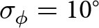 $\sigma_\phi = 10{^\circ}$ and the amplitude error with a standard deviation of
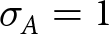 $\sigma_A = 1$ dB, representing realistic tolerances for a millimeter-wave feeding network operating at 28 GHz. Three test cases were evaluated independently: phase errors only, amplitude errors only, and a combined case in which both types of error were applied simultaneously. For each simulation scenario, the mean response and the envelope over all realizations are reported.
BINDER MKF 56 dynamic climate chamber used for the thermal cycling characterization of the EDA array prototype.

Time distribution of the individual thermal cycle in the mechanical reliability test of the proposed EDA array.

Figure A1 shows the resulting array radiation patterns for various scanning angles along both the 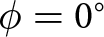 $\phi = 0{^\circ}$ and
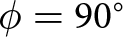 $\phi = 90{^\circ}$ vertical cut-planes. As expected from the zero-mean Gaussian error model, the mean pattern across all realizations closely follows the ideal case for every scanning angle. The main beam is largely unaffected by the applied errors, which can be attributed to the spatial averaging effect of the large 64-element array, where uncorrelated element-level perturbations partially cancel in the far field. The sidelobe region, however, exhibits greater sensitivity to both phase and amplitude errors, with individual realizations showing sidelobe levels elevated above the ideal pattern. This behavior is consistent with established phased array theory, where random element errors are known to raise the average sidelobe level while leaving the main beam gain and direction largely intact [Reference Ruze36].
Magnitude of the reflection coefficient as measured at the input of the central EDA array element before and after the thermal cycling test.

Thermal cycling characterization
To further understand the robustness of the presented design against real-life environments, a thermal cycling test was performed on the EDA array in accordance with IEC 60068-2-14 [37]. This standard specifies procedures for assessing the ability of components and assemblies to withstand exposure to repeated temperature extremes with a controlled transition rate.
The thermal cycling tests were carried out using a BINDER MKF 56 dynamic climate chamber [38], shown in Figure A2. This chamber features a 60-liter stainless-steel interior with internal dimensions of  $400 \times 420 \times 348$ mm, which comfortably accommodates the
 $8 \times 8$ EDA array prototype. The MKF 56 supports a temperature range of
 $-40 {^\circ}\text{C}$ to
 $+180 {^\circ}\text{C}$ with average heating and cooling rates of 5 K/min (per IEC 60068-3-5), a temperature fluctuation of
 $\pm 0.1$ to
 $\pm 0.5$ K depending on the setpoint, and a temperature variation of
 $\pm 0.5$ to
 $\pm 1.5$ K. The chamber employs APT.lineTM preheating chamber technology to ensure homogeneous thermal conditions throughout the test volume, and is equipped with a controller that allows time-segment programming of custom thermal profiles with adjustable ramp functions. Temperature monitoring is performed by means of an internal Pt 100 sensor, while thermal insulation is provided by CFC-free PUR foam. These specifications ensure that the thermal cycling parameters prescribed by IEC 60068-2-14 are met with sufficient margin across the entire test volume.
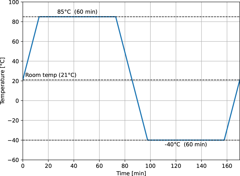
The EDA array prototype was placed inside the chamber on a stainless-steel rack and subjected to five complete thermal cycles between  $-40{^\circ}$C and
 $+85{^\circ}$C. Each cycle consisted of a controlled ramp from room temperature to the upper extreme of
 $+85{^\circ}$C at a rate of
 $5{^\circ}$C/min, a dwell time of 60 minutes at
 $+85{^\circ}$C, a controlled ramp down to
 $-40{^\circ}$C at
 $5{^\circ}$C/min, a dwell time of 60 minutes at
 $-40{^\circ}$C, and a final return ramp to room temperature. The time profile of a single thermal cycle is shown in Figure A3. This profile was programmed directly into the MKF 56 controller and executed automatically for five consecutive cycles without interruption.
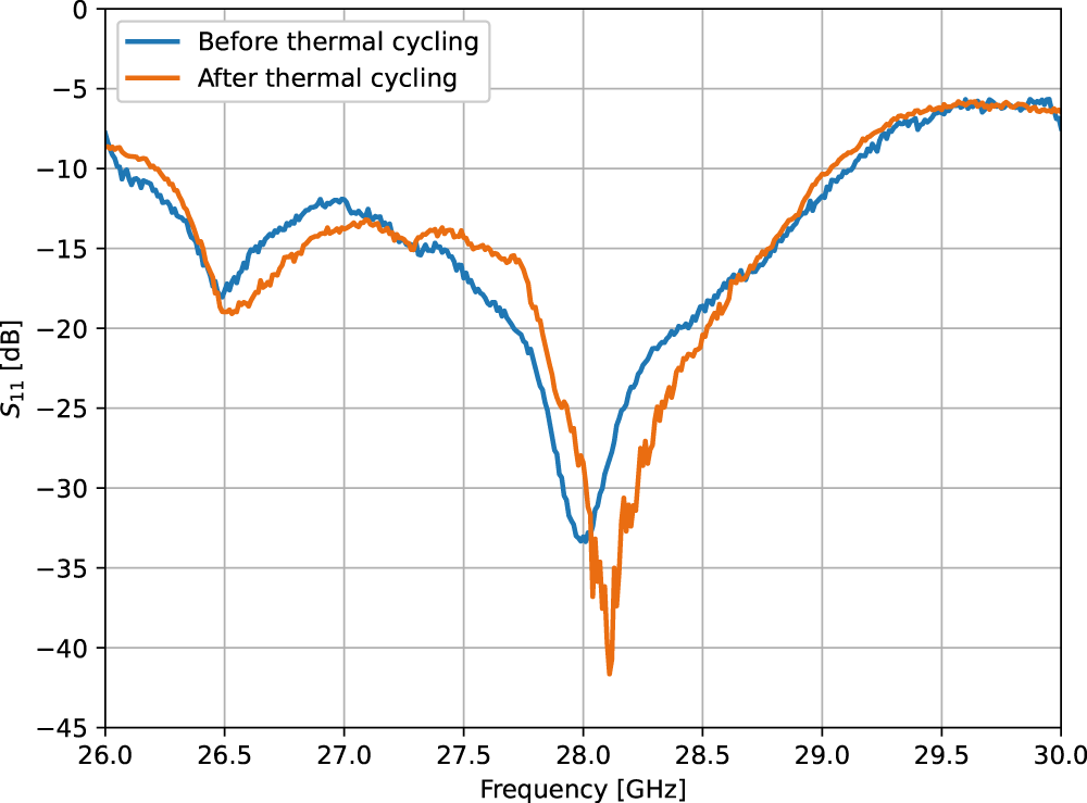
To assess any degradation in RF performance caused by the thermal cycling, the  $S_{11}$ of a central array element was measured before and after the complete five-cycle sequence using a VNA. The results are compared in Figure A4. The measured response remains consistent after thermal cycling, with no significant frequency shift or impedance degradation observed. The minor differences between the two traces are attributed to measurement repeatability and connector repositioning between the pre- and post-cycling measurements. These results confirm that the layered CNC-machined aluminum construction of the EDA array, including the bolted assembly and the PCB-based launcher interface, is mechanically robust against the thermal stresses induced by repeated cycling over a
 $125{^\circ}$C temperature range.




















 Open access

