



1 Introduction
We consider Gibbs states on sequence spaces, that is, probability measures for which there is a specified set of functions that determine the probabilities of configurations on any finite subset conditioned on the configuration outside that subset. Let
$X=S^I$
 be a sequence space, where S is a finite set with the discrete topology, and I is a countable (infinite) set. The topology on X is the product topology, with respect to which X is compact, and
${\mathcal B}$
 denotes the corresponding Borel
$\sigma $
 -algebra. If
$x\in S^{\Lambda ^\prime }\, (\Lambda ^\prime \subseteq I)$
 and
$\Lambda \subseteq \Lambda ^\prime $
 , then
$x_\Lambda $
 denotes the natural projection of x onto
$S^\Lambda $
 and
$[x]_\Lambda $
 is the cylinder set
${\{y\in X:y_\Lambda =x_\Lambda \}}$
 ; similarly, if
$s\in S$
 and
$i\in I$
 ,
$[s]_i$
 denotes
$\{y\in X:y_i=s\}$
 . The sub-
$\sigma $
 -algebra of
${\mathcal B}$
 generated by
$\{[x]_\Lambda : x\in X\}$
 is denoted by
${\mathcal B}_\Lambda $
 , and
${\mathcal C}$
 denotes the set of finite, non-empty subsets of I.
A specification on X is a collection
${\mathcal V}=\{\phi _\Lambda \}_{\Lambda \in {\mathcal C}}$
 of non-negative Borel functions on X such that, for all
$\Lambda \in {\mathcal C}$
 and
$x\in X$
 ,

and for
$K\subseteq \Lambda $
 ,

The specification
${\mathcal V}$
 is said to be continuous if
$\phi _\Lambda $
 is continuous for all
$\Lambda \in {\mathcal C}$
 , and positive if
$\phi _\Lambda>0$
 for all
$\Lambda \in {\mathcal C}$
 . If
$I={\mathbb Z}^d\, (d\geq 1)$
 , then
$T=\{T_i\}_{i\in I}$
 denotes the d-dimensional shift on X, that is,
$(T_ix)_j=x_{i+j}\, (x\in X,\ i,j\in {\mathbb Z}^d)$
 , and
${\mathcal V}$
 is said to be T-invariant if
$\phi _{i+\Lambda }(x)=\phi _\Lambda (T_ix)$
 for all
$i\in {\mathbb Z}^d$
 and
$\Lambda \in {\mathcal C}$
 . (As usual, when
$d=1$
 , we equate T with
$T_1$
 .)
A probability measure
$\mu $
 on
$(X,{\mathcal B})$
 is a Gibbs state for a specification
${\mathcal V}=\{\phi _\Lambda \}_{\Lambda \in {\mathcal C}}$
 if

for all
$\Lambda \in {\mathcal C}$
 (by a.e., we mean almost everywhere). The set of Gibbs states is denoted by
${\mathcal G}({\mathcal V})$
 .
If
${\mathcal V}$
 is continuous, there exists at least one Gibbs state, and natural questions concern the structure of
${\mathcal G}({\mathcal V})$
 , in particular, uniqueness and any ergodic or mixing properties of Gibbs states. In general,
${\mathcal G}({\mathcal V})$
 is a compact, convex subset of
$M(X)$
 (the set of probability measures on
$(X,{\mathcal B})$
 ), and its extreme points are those states for which the tail
$\sigma $
 -field
$\bigcap _{\Lambda \in {\mathcal C}}{\mathcal B}_{\Lambda ^c}$
 is trivial. If, in addition,
$I={\mathbb Z}^d$
 and
${\mathcal V}$
 is T-invariant, then at least one of the Gibbs states is T-invariant; the T-invariant Gibbs states form a convex subset of
${\mathcal G}(V)$
 , the extreme points of which are the ergodic ones. Thus, a unique T-invariant Gibbs state
$\mu $
 is necessarily ergodic, but if it is also the only Gibbs state, then it follows from the triviality of the tail field that
$(T,\mu )$
 has some strong mixing properties. However, from the dynamical systems perspective, the system with the strongest mixing properties is one that is isomorphic to, and hence indistinguishable from, a Bernoulli shift (by which we mean the invertible dynamical system generated by a sequence of independent identically distributed random variables taking values in a finite set). While it is known that for those specifications that are attractive (or ferromagnetic), uniqueness of the Gibbs state implies the Bernoulli property (see [Reference Adams1, Reference Hulse12, Reference Hulse13]), in general, this is not the case.
Dobrushin [Reference Dobrushin7] showed that if
${\mathcal V}=\{\phi _\Lambda \}_{\Lambda \in {\mathcal C}}$
 is a continuous specification such that

then
${\mathcal V}$
 has a unique Gibbs state
$\mu $
 . This result holds for all countable I and does not depend on I having a group structure. If
$I={\mathbb Z}^d$
 (in fact, if I is any amenable group) and
${\mathcal V}$
 is T-invariant, then
$\mu $
 is T-invariant and the corresponding dynamical system
$(T,\mu )$
 is Bernoulli (see [Reference Hulse13]).
Of particular interest in statistical mechanics are those specifications determined by an interaction potential
$\Phi =\{\Phi _\Lambda \}_{\Lambda \in {\mathcal C}}$
 , that is, a set of functions on X such that
$\Phi _\Lambda $
 is
${{\mathcal B}}_\Lambda $
 -measurable. The corresponding specification
${\mathcal V}_\Phi $
 is given by

where

Usually,
$\Phi $
 is required to satisfy a summability condition that ensures
$H^\Phi _\Lambda $
 is continuous, and hence that
${\mathcal V}_\Phi $
 is continuous and positive. When
$I={\mathbb Z}^d$
 , the interaction potential
$\Phi $
 is said to be T-invariant if
$\Phi _{\Lambda +i}(x)=\Phi _\Lambda (T_ix)$
 for all
$\Lambda \in {\mathcal C}$
 and
$i\in {\mathbb Z}^d$
 , in which case,
${\mathcal V}_\Phi $
 is also T-invariant. An example that has been studied extensively is the well-known Ising model on
$\{-1,1\}^{{\mathbb Z}^d}$
 , where
$\Phi _\Lambda \equiv 0$
 for
$|\Lambda |\neq 2$
 . In particular, we note that in dimensions
$d\geq 2$
 , the nearest-neighbour model (where
$\Phi _{\{i,j\}}\equiv 0$
 unless
$|i-j|=1$
 ) gives examples of non-unique Gibbs states. When
$d=1$
 , the situation is quite different. Here, the nearest-neighbour model has a unique Gibbs state; more generally, if
$\Phi _{\{i,j\}}(x)=-J(|i-j|)x_ix_j$
 , where
$\{J(n)\}$
 is a non-negative sequence, there is a unique Gibbs state provided
$\sum _{i=1}^niJ(i)=o(\sqrt {\log n})$
 [Reference Rogers and Thompson17]. In contrast, if
$J(n)=\beta n^{-\alpha }$
 , there is a phase transition (that is, non-uniqueness) for large enough
$\beta $
 when
$1<\alpha \leq 2$
 [Reference Fröhlich and Spencer9]. (A more thorough survey of such results can be found in [Reference Georgii11].)
For potentials in general, Ruelle [Reference Ruelle19] showed that when
$I={\mathbb Z}$
 and
$\Phi =\{\Phi _\Lambda \}_{\Lambda \in {\mathcal C}}$
 is T-invariant, there is a unique T-invariant Gibbs state provided

Gallavotti [Reference Gallavotti10] and Ledrappier [Reference Ledrappier16] independently proved it has the Bernoulli property. Coelho and Quas [Reference Coelho and Quas6] pointed out that by combining Ruelle’s characterization [Reference Ruelle18] of the T-invariant Gibbs states of
$\Phi $
 as equilibrium states of the function

with the results of Walters [Reference Walters21], (1.4) could be replaced by the weaker hypothesis

Berbee [Reference Berbee3] considered continuous specifications
$\{\phi _\Lambda \}_{\Lambda \in {\mathcal C}}$
 determined as follows. There is a sequence
$\{\Lambda _n\}_{n=0}^\infty \subset {\mathcal C}$
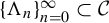 such that
$\Lambda _n\nearrow I$
 and positive
${\mathcal B}_{\Lambda _{n-1}^c}$
 -measurable functions
$f_n\in C(X)\, (n\geq 0)$
 (with
$\Lambda _{-1}=\emptyset $
 ) such that

Any positive continuous specification can be described in this way (see §2). For a positive function f on X and
$\Lambda \subseteq I$
 , let

(Note that
$\bar r_\Lambda (f)=r_\Lambda (f)^{-1}$
 .) Berbee showed that if

then there is a unique Gibbs state. Like Dobrushin’s result, this holds for any countable I and for non-invariant, as well as invariant, specifications. Taking
$I={\mathbb Z}$
 and

(here and later, we use the usual notation for an interval
${\mathcal I}\subseteq {\mathbb R}$
 to denote
${\mathcal I}\cap {\mathbb Z}$
 ), and comparing hypotheses for the relevant
$f_n$
 for an interaction potential (2.7), it can be seen that Berbee’s hypothesis is weaker than Ruelle’s (1.4); however, while in some cases it is weaker than that of Coelho and Quas (1.5), in others, it is not.
The hypotheses (1.4)–(1.5) can be viewed as measures of the continuity of
$A(\Phi )$
 in terms of its variation on sites outside finite subsets, or equivalently, in terms of the rate at which
$\|\phi _\Lambda \|$
 decreases as
$\text {diam}(\Lambda )$
 increases. Similarly, (1.6) is a measure of the continuity of the functions
$f_n$
 , which, in the case of an interaction potential
$\Phi $
 with the
$f_n$
 defined by (2.7), is also related to the continuity of
$A_\Phi $
 . In this paper, we consider whether this type of continuity hypothesis can be relaxed. We restrict our attention to the case
$I={\mathbb Z}$
 since (1.4) and (1.5) are only valid in this case, and while Berbee’s result holds for any I, in the case of T-invariant specifications, it would seem that (1.6) rules out any genuinely multi-dimensional examples. Indeed, as has already been noted, the nearest-neighbour Ising model provides examples of non-uniqueness in dimensions greater than one. From hereon, X denotes
$S^{\mathbb Z}$
 .
As Dobrushin [Reference Dobrushin7] pointed out, any positive specification
${\mathcal V}=\{\phi _\Lambda \}_{\Lambda \in {\mathcal C}}$
 is completely determined by
$\{\phi _{\{n\}}:n\in {\mathbb Z}\}$
 ; consequently, if
${\mathcal V}$
 is also T-invariant, it is determined by
$\phi _{\{0\}}$
 alone. Thus, it seems natural to seek conditions for uniqueness and Bernoullicity in terms of
$\phi _{\{0\}}$
 , or equivalently, the ratios
$\{\phi _{\{0\}}(s_0x)/\phi _{\{0\}}(t_0x)\colon s,t\in S,\,x\in X\}$
 , where
$s_nx\in X\, (s\in S,\,x\in X,\,n\in {\mathbb Z})$
 is defined by

We show the following theorem.
Theorem 1.1. Let
${\mathcal V}=\{\phi _\Lambda \}_{\Lambda \in {\mathcal C}}$
 be a positive, continuous, T-invariant specification on X, and let

for some
$s\in S$
 . If, for some
$0<\alpha \leq 1$
 ,

and

then
${\mathcal V}$
 has a unique Gibbs state
$\mu $
 , which is T-invariant, and
$(T,\mu )$
 is Bernoulli.
In particular, there is a unique, Bernoulli Gibbs state if

for some
$\beta <1/2$
 and non-negative series
$\sum a_n<\infty $
 . In fact, we prove Theorem 1.1 under slightly weaker hypotheses (Theorem 5.1), which allows the following version to be deduced when the specification is given in terms of an interaction potential.
Theorem 1.2. Let
$\Phi =\{\Phi _\Lambda \}_{\Lambda \in {\mathcal C}}$
 be a T-invariant interaction potential on X. If

for some
$\beta <1/2$
 and
$a_n\geq 0$
 such that
$\sum a_n<\infty $
 , then
$\Phi $
 has a unique Gibbs state
$\mu $
 , which is T-invariant, and
$(T,\mu )$
 is Bernoulli.
This includes all interaction potentials satisfying (1.4). In some cases, such as when
$\sup \{|\Lambda | :\Phi _\Lambda \not \equiv 0\}<\infty $
 , (1.8) is also weaker than (1.5), but in others, it is not. Comparison with (1.6) is less straightforward, since (1.6) applies to non-invariant specifications and arbitrary increasing sequences
$\{\Lambda _n\}_{n=0}^\infty \subset {\mathcal C}$
 . Consideration of the Ising model suggests Theorems 1.1 and 1.2 can give better results for uniqueness in some cases, but the main difference is that the Bernoulli property is obtained.
The idea of the proof of Theorem 5.1 is to characterize a Gibbs state
$\mu $
 in terms of its conditional probabilities

in other words, as a g-chain; uniqueness, T-invariance and the Bernoulli property can then be determined from similar results for g-chains. Here, we use a result (Theorem 4.5) that is a formulation based on the techniques of Johansson, Öberg and Pollicott [Reference Johansson, Öberg and Pollicott15]. The estimate of the variation of
$\log g$
 needed for Theorem 4.5 is provided by Theorem 4.2. This result may be of some interest in its own right as it gives a sufficient condition for the set of Gibbs states of a T-invariant specification to be the set of g-chains for some continuous function g. (A characterization of g-chains which are also Gibbs states, as well as a discussion of the problem of determining whether a Gibbs state is a g-chain, can be found in [Reference Berghaut, Fernandez and Verbitskiy5].) Theorem 4.2 follows from Proposition 4.1, which gives a general criterion for the set of Gibbs states to be the same as the set of g-chains for some continuous function g, and Proposition 3.1, which is an adaptation of Berbee’s method of ratio bounds in [Reference Berbee3].
Lastly, we consider some alternative hypotheses which guarantee a unique T-invariant Gibbs state, but not the Bernoulli property.
2 Specifications and Gibbs states
We start with some preliminary remarks about specifications and Gibbs states; a more detailed account can be found in [Reference Georgii11], for example. The following notation will be used throughout: if
$x\in S^{\Lambda _1}$
 ,
$y\in S^{\Lambda _2}$
 are sequences and
$\Lambda _1\cap \Lambda _2=\emptyset $
 , then
$xy\in S^{\Lambda _1\cup \Lambda _2}$
 denotes the sequence such that

The set of bounded Borel functions on X is denoted by
$B(X)$
 .
Let
$X=S^{\mathbb Z}$
 be a sequence space as described in the introduction, and let
${{\mathcal V}=\{\phi _\Lambda \}_{\Lambda \in {\mathcal C}}}$
 be a specification on X. Then
${\mathcal V}$
 determines a set of probability measures
$\pi ^{\mathcal V}_\Lambda (\,\cdot \,|\,x)\, (\Lambda \in ~{\mathcal C},\ x\in X)$
 as follows:

and
$\mu \in {\mathcal G}({\mathcal V})$
 if and only if

Thus, if
${\mathcal V}$
 is continuous,
${\mathcal G}({\mathcal V})$
 is closed (in the weak-* topology), and moreover, any weak-* limit of measures of the form

is a Gibbs state for
${\mathcal V}$
 . Since
$M(X)$
 is compact, it follows that there is at least one Gibbs state
$\mu $
 and the uniqueness of
$\mu $
 is equivalent to the uniform convergence (for each
${f\in C(X)}$
 ) of
$\pi ^{\mathcal V}_\Lambda (f\,|\,x)$
 to
$\mu (f)$
 as
$\Lambda \nearrow {\mathbb Z}$
 .
Similarly, if
${\mathcal V}$
 is T-invariant, any weak-* limit of measures of the form

is a T-invariant Gibbs state for
${\mathcal V}$
 . By compactness, there is always one such measure
$\mu $
 and its uniqueness is equivalent to

uniformly in x for all
$f\in C(X)$
 .
Note that if
$\phi _\Lambda $
 is given for some
$\Lambda \in {\mathcal C}$
 , then (1.2) determines
$\phi _K$
 for all
$K\subseteq \Lambda $
 . Moreover, if (1.2) holds for the pairs
$K,\Lambda $
 and
$K',K$
 , where
$K'\subseteq K\subseteq \Lambda $
 , then it holds for
$K',\Lambda $
 . Thus, to define a specification, it is enough to consider a sequence
$\{\Lambda _n\}_{n=0}^\infty \subset {\mathcal C}$
 such that
$\Lambda _n\nearrow {\mathbb Z}$
 , and specify the
$\phi _{\Lambda _n}$
 so that (1.1) and (1.2) hold for
$\Lambda _{n-1},\Lambda _n\, (n\geq 1)$
 .
Let
${\mathcal V}$
 be positive; note that for positive specifications, (1.2) is equivalent to

If
$\Lambda \in {\mathcal C}$
 and
$\{i_0,\ldots ,i_n\}$
 is an enumeration of
$\Lambda $
 , with
$\Lambda _j=\{i_0,\ldots ,i_j\}$
 (
$0\leq j\leq n$
 ), then for any
$x,x^*\in X$
 , we have

and so it follows that

(Here and later,
$\Lambda _{-1}$
 is taken to be
$\emptyset $
 .) This, together with (1.1), determines
$\phi _\Lambda $
 . In particular, any positive specification
${\mathcal V}=\{\phi _\Lambda \}_{\Lambda \in {\mathcal C}}$
 is completely determined by the
$\phi _{\{n\}}\, (n\in {\mathbb Z})$
 . Moreover,
${\mathcal V}$
 is T-invariant provided
$\phi _{\{n\}}=\phi _{\{0\}}\circ T^n$
 for all
$n\in {\mathbb Z}$
 , in which case, it is determined solely by
$\phi _{\{0\}}$
 .
Conversely, given a sequence of positive functions
$\{\phi _{\{n\}}\}_{n\in {\mathbb Z}}\subset B(X)$
 such that
$\sum _{y\in [x]_{\{n\}}}\phi _{\{n\}}(y)=1$
 for all
$x\in X$
 , and
$\{\Lambda _n\}_{n=0}^\infty \subset {\mathcal C}$
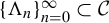 such that
$\Lambda _n\nearrow {\mathbb Z}$
 and
${|\Lambda _n\setminus \Lambda _{n-1}|=1\, (n\geq 0)}$
 , define
$\phi _{\Lambda _n}$
 by (1.1) and

where
$\{i_n\}=\Lambda _n\setminus \Lambda _{n-1}$
 . Clearly, the
$\phi _{\Lambda _n}$
 satisfy (2.1) and so determine a specification, which is independent of the choice of
$\{\Lambda _n\}$
 since a specification is determined solely by the
$\phi _{\{n\}}$
 . Thus, any sequence of positive functions
$\{\phi _{\{n\}}\}_{n\in {\mathbb Z}}\subset B(X)$
 such that
$\sum _{y\in [x]_{\{n\}}}\phi _{\{n\}}(y)=1$
 for all
$x\in X$
 determines a unique positive specification. In particular, any positive
$f\in B(X)$
 determines a (unique) T-invariant specification
${{\mathcal V}=\{\phi _\Lambda \}_{\Lambda \in {\mathcal C}}}$
 such that

By a specification sequence, we mean a sequence
$\{\Lambda _n,f_n\}_{n=0}^\infty \subset {\mathcal C}\times B(X)$
 such that
$\Lambda _{n-1}\subset \Lambda _n$
 ,
$|\Lambda _n\setminus \Lambda _{n-1}|=1$
 , and
$f_n$
 is positive and
${\mathcal B}_{\Lambda _{n-1}^c}$
 -measurable; it is a specification sequence for the specification
${\mathcal V}=\{\phi _\Lambda \}_{\Lambda \in {\mathcal C}}$
 if

If
${\mathcal V}$
 is positive, such a sequence exists for any choice of
$\{\Lambda _n\}$
 . Indeed, let
$x^*\in X$
 and define

where
$\Lambda _n\setminus \Lambda _{n-1}=\{i_n\}$
 . Then
$f_n$
 is suitably measurable, and it follows from (2.2) that (2.3) holds. If
${\mathcal V}$
 is continuous, so are the
$f_n$
 , and if
${\mathcal V}$
 is also T-invariant, then a consequence of (2.4) is that if

for some
$s\in S$
 , then a specification sequence
$\{[0,n],f_n\}_{n=0}^\infty $
 can be chosen so that
$f_0=f$
 and

Conversely, any specification sequence
$\{\Lambda _n,f_n\}_{n=0}^\infty $
 such that
$\Lambda _n\nearrow {\mathbb Z}$
 determines a (unique) specification
${\mathcal V}=\{\phi _\Lambda \}_{\Lambda \in {\mathcal C}}$
 via (2.3), since (2.1) holds for the pairs
$\Lambda _{n-1}$
 ,
$\Lambda _n$
 .
Any positive, continuous, T-invariant specification
${\mathcal V}$
 can be determined by a T-invariant interaction potential
$\Phi =\{\Phi _\Lambda \}_{\Lambda \in {\mathcal C}}$
 such that for some
$s\in S$
 ,

(see [Reference Sullivan20] for details). If
$\sum _{\Lambda \ni 0}\|\Phi _\Lambda \|<\infty $
 , the functions

determine a specification sequence
$\{[0,n],f_n\}_{n=0}^\infty $
 for
${\mathcal V}$
 , and since
$\Phi $
 is T-invariant,

3 A ratio bound
Given a specification sequence
$\{[0,n],f_n\}_{n=0}^\infty $
 , define
$L_{m,n}\colon B(X)\rightarrow B(X)\, (0\leq m\leq n)$
 by

and let

In addition to the usual notation for sets of integers, we denote the sets of negative and non-positive integers by
${\mathbb N}^-$
 and
${\mathbb Z}^-$
 , respectively.
Proposition 3.1. Let
$\{[0,n],f_n\}_{n=0}^\infty $
 be a specification sequence,
$A\subseteq {\mathbb N}^-$
 , and

Then

We split the proof of Proposition 3.1 into two lemmas. The proof of the first one is based on that of [Reference Berbee3, Proposition 2.1].
Lemma 3.2. Let
$\{f_n\}_{n=0}^\infty \subset B(X)$
 and A be as above, and let
$x,y\in X$
 be such that
${x_A=y_A}$
 . If
$\{v_k\}_{k=0}^\infty $
 is an increasing, positive sequence such that

then

Proof. We denote
$\rho _k^{(n)}(x,y)$
 by
$\rho _k^{(n)}$
 , and
$[\zeta ]_{[i,j]}$
 by
$[\zeta ]_i^j$
 (
$\zeta \in S^\Lambda $
 ,
$[i,j]\subseteq \Lambda \subseteq {\mathbb Z}$
 ). Let

and

Note that

and

Let
$m\geq 0$
 ,
$n\geq 1$
 and
$\zeta \in S^{[m,m+k]}$
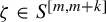 for some
$0\leq k\leq n$
 . Since
$f^{(j)}_m(w)$
 ,
$\phi _{m}^{(j)}(w)$
 depend only on
$w_{[m,m+j]}$
 , we can identify them with the functions induced by the natural projection onto
$S^{[m,m+j]}$
 . Then

and

Therefore,

for
$0\leq k\leq n-1,\,m\geq 0$
 , and

for
$k=n\geq 1$
 . Hence,

(where the empty sum is taken to be 0). Rearranging, we have

as required.
Now, given an increasing sequence
$\{v_k\}_{k=0}^\infty $
 such that
$0<v_k\leq 1$
 for all k, consider
$p_k^{(n)}\, (-1\leq k\leq n,\,n\geq 0)$
 , defined recursively by


(As before, when
$k=n$
 , the empty sum is taken to be 0.)
Lemma 3.3. Let
$p_k^{(n)}\, (k\geq -1,\,n\geq 0)$
 and
$\{v_k\}_{k=0}^\infty $
 be as above. Then

Proof. It follows from (3.3) that for
$0\leq k\leq n$
 ,
$n\geq 1$
 ,


Hence, if
$n{\kern-1pt}\geq{\kern-1pt} 1$
 , then
$p^{(n+1)}_k{\kern-1pt}\geq{\kern-1pt} p^{(n)}_k$
 for
$0{\kern-1pt}\leq{\kern-1pt} k{\kern-1pt}\leq{\kern-1pt} n$
 provided
$p^{(n)}_k\geq p^{(n-1)}_k$
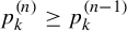 for
$0{\kern-1pt}\leq{\kern-1pt} k{\kern-1pt}\leq{\kern-1pt} n{\kern-1pt}-{\kern-1pt}1$
 . Since
$p^{(1)}_0\geq p^{(0)}_0$
 , it follows inductively that
$p_k^{(n+1)}\geq p_k^{(n)}$
 for all
$0\leq k\leq n$
 . Thus,

is well defined, and

Therefore,

and so

Summing gives

Since
$p_{n+1}\geq 0$
 ,

from which the result follows.
Proof of Proposition 3.1.
It follows from Lemma 3.2 and the Cauchy–Schwarz inequality that

for any
$x,y\in X$
 such that
$x_A=y_A$
 . Note also that
$\rho _{-1}^{(n)}(x,y)\rho _{-1}^{(n)}(y,x)=1$
 for all
$n\geq 0$
 and
$x,y\in X$
 . Define
$p^{(n)}_k\, (-1\leq k\leq n,\,n\geq 0)$
 inductively as in (3.1)–(3.3) with
$\{v_k\}$
 as in the statement of Proposition 3.1. Then it follows from (3.1)–(3.4) that

The result now follows from Lemma 3.3.
4 Gibbs states and g-chains
Let

and let
$g\in {\mathcal G}_X$
 . A measure
$\mu \in M(X)$
 is a g-chain if

for all
$n\in {\mathbb Z}$
 . A T-invariant g-chain is usually referred to as a g-measure. If
$g\in {\mathcal G}_X$
 is continuous, there is always at least one g-measure.
Proposition 4.1. Let
${\mathcal V}=\{\phi _\Lambda \}_{\Lambda \in {\mathcal C}}$
 be a positive, continuous, T-invariant specification. If
$\pi ^{\mathcal V}_{[0,n]}([x]_{\{0\}}\,|\,x)$
 converges to a continuous limit in
$x\in X$
 as
$n\to \infty $
 , then

is a positive, continuous function in
${\mathcal G}_X$
 , and
$\mu \in {\mathcal G}({\mathcal V})$
 if and only if
$\mu $
 is a
$g_{\mathcal V}$
 -chain.
Proof. Let

as above; by hypothesis,
$g_{\mathcal V}$
 is continuous. Note that
$g_{\mathcal V}(x)$
 is
${\mathcal B}_{{\mathbb Z}^-}$
 -measurable, and since

it follows that
$g_{\mathcal V}$
 is positive. Clearly,
$\sum _{s\in S}g_{\mathcal V}(s_0x) =1$
 for all
$x\in X$
 , and so
$g_{\mathcal V}\in {\mathcal G}_X$
 . Moreover, it follows from the Martingale theorem that

for any Gibbs state
$\mu $
 of
${\mathcal V}$
 when
$n=0$
 , and hence, by the T-invariance of
${\mathcal V}$
 , for all
$n\in {\mathbb Z}$
 ; thus, any Gibbs state is a
$g_{\mathcal V}$
 -chain.
Conversely, if
$\mu $
 is a
$g_{\mathcal V}$
 -chain, then

Given
$n\in {\mathbb Z}$
 , consider
$k>m>n$
 . From (4.1), we have

for all
$x\in X$
 . Therefore, for all
$s,t\in S$
 ,
$x\in X$
 ,

It follows that
$\mu ([s]_n\,|\,{\mathcal B}_{\{n\}^c})(x)=\phi _{\{n\}}(s_nx)$
 a.e.
$(\mu )$
 for all
$s\in S$
 ,
$n\in {\mathbb Z}$
 , and so
$\mu \in {\mathcal G}({\mathcal V})$
 .
Theorem 4.2. Let
${\mathcal V}=\{\phi _\Lambda \}_{\Lambda \in {\mathcal C}}$
 be a positive, continuous, T-invariant specification with specification sequence
$\{[0,n],f_n\}_{n=0}^\infty $
 . If

then

is well defined, the convergence is uniform in x, and it determines a positive function
$g_{\mathcal V}\in {\mathcal G}_X\cap C(X)$
 such that

where

Moreover,
$\mu \in {\mathcal G}({\mathcal V})$
 if and only if
$\mu $
 is a
$g_{\mathcal V}$
 -chain.
Proof. Given
$\{f_n\}$
 , let
$\rho ^{(n)}_k(\,\cdot \,,\,\cdot \,)$
 be as in §3. Note that

Then since
${\mathcal V}$
 is positive and continuous, Proposition 3.1 (with
$A={\mathbb N}^-$
 ) implies that

Given
$x\in X$
 , consider the sequences

which are respectively decreasing, increasing in n and, hence, convergent. It follows from (4.2) that they converge to the same limit, and so

is well defined for all
$x\in X$
 . Furthermore,

and so the convergence is uniform. Thus, the limit is continuous, and it follows from Proposition 4.1 that
$g_{\mathcal V}\in {\mathcal G}_X$
 ,
$g_{\mathcal V}$
 is positive, and
$\mu \in {\mathcal G}({\mathcal V})$
 if and only if
$\mu $
 is a
$g_{\mathcal V}$
 -chain.
Applying Proposition 3.1 again with
$A=[-n,-1]$
 (and
$\{f_n\}$
 as before) gives

as required.
Remark 4.3. Proposition 4.1 and Theorem 4.2 can easily be generalized to include non-invariant specifications
${\mathcal V}$
 , in which case,
$g_{\mathcal V}$
 is replaced by a sequence of continuous functions
$\{g_n\}_{n=-\infty }^\infty $
 such that

Note that, in general,
$g_n(x)\neq g_0(T^nx)$
 .
The following result will be useful for estimating the variation of
$g_{\mathcal V}$
 .
Lemma 4.4. Let
${\mathcal V}=\{\phi _\Lambda \}_{\Lambda \in {\mathcal C}}$
 be a positive, continuous, T-invariant specification with specification sequence
$\{[0,n],f_n\}_{n=0}^\infty $
 . If

for some
$0<\alpha \leq 1,\,0<K<\infty $
 , then

is well defined, and

Proof. Note that (4.3) implies

and so it follows from Theorem 4.2 that
$g_{\mathcal V}\in {\mathcal G}_X$
 is well defined and

where

as before. Note that

where

Note also that
$a_n$
 is decreasing and the power series
$\sum _{k=1}^\infty a_kt^k$
 is convergent for
$0\leq t<1$
 . For such series, we have the following Tauberian theorem (see [Reference Feller8, p. 447]): for
$0<\alpha <\infty $
 ,

Thus, if

where
$0<\alpha \leq 1$
 ,
$0<K<\infty $
 , then

and since
$1-t\sim |\log t|$
 as
$t\nearrow 1$
 , and
$t_n\nearrow 1$
 as
$n\to \infty $
 , it follows from (4.4) that

as required.
The next result follows from the results and techniques of Johansson, Öberg and Pollicott in [Reference Johansson, Öberg and Pollicott15], although it is not formulated there; for an explicit proof, see [Reference Hulse14].
Theorem 4.5. Let
$g\in {\mathcal G}_X$
 be positive and continuous. If

for some
$\unicode{x3bb}>1$
 , then there is a unique g-chain
$\mu \in M(X)$
 , which is T-invariant and Bernoulli.
Note that if (4.5) holds for some
$\unicode{x3bb}>1$
 , then it holds for all such
$\unicode{x3bb} $
 .
5 Proof of the main results
Theorem 5.1. Let
${\mathcal V}=\{\phi _\Lambda \}_{\Lambda \in {\mathcal C}}$
 be a positive, continuous, T-invariant specification on X with specification sequence
$\{[0,n],f_n\}_{n=0}^\infty $
 . If, for some
$0<\alpha \leq 1$
 ,

and

then
${\mathcal V}$
 has a unique Gibbs state
$\mu $
 , which is T-invariant, and
$(T,\mu )$
 is Bernoulli.
Proof. It follows from (5.1), Theorem 4.2 and Lemma 4.4 that there is a positive, continuous
$g_{\mathcal V}\in {\mathcal G}_X$
 such that any Gibbs state for
${\mathcal V}$
 is a
$g_{\mathcal V}$
 -chain and

Theorem 1.1 follows immediately from Theorem 5.1 and (2.5)–(2.6). If the specification is described in terms of an interaction potential
$\Phi =\{\Phi _\Lambda \}_{\Lambda \in {\mathcal C}}$
 , then it follows from (2.7) and (2.8) that (5.1) and (5.2) hold provided there are constants
$K>0$
 and
$0<\alpha \leq 1$
 such that

and

This will be the case if

for some
$1/2<\alpha \leq 1$
 and
$\sum a_n<\infty $
 , that is, if (1.8) holds with
$\beta =1-\alpha $
 ; thus, Theorem 1.2 follows.
Since

Theorem 1.2 includes potentials satisfying (1.4). Comparison with (1.5) and (1.6) is less straightforward; in some cases, its hypotheses are weaker, but not always. Note however that Theorem 1.2 guarantees a unique Gibbs state (absence of symmetry breakdown), whereas (1.5) only guarantees uniqueness of T-invariant Gibbs states, and (1.6) does not include the Bernoulli property.
By way of comparison, consider the Ising model on
$\{-1,1\}^{\mathbb Z}$
 with pair interactions

where
$\beta>0$
 (the inverse temperature) is a constant and
$|J(n)|\leq n^{-\alpha }$
 for some
$\alpha>1$
 . Since Berbee’s result applies to non-invariant specifications and does not depend on any group structure, there is no loss of generality in assuming that
$I={\mathbb Z}$
 and

(as in (1.7)), other than the assumption that
$|\Lambda _n\setminus \Lambda _{n-1}|=1$
 .
The corresponding specification sequence
$\{\Lambda _n,f_n\}$
 is given by

where
$i_n$
 is the unique element of
$\Lambda _n\setminus \Lambda _{n-1}$
 . Note that
$\inf _{i\geq 0}\bar r_{\Lambda _{i+k}}(f_i)=\bar r_{\Lambda _k}(f_0)$
 ,

and

Thus, for
$\alpha>2$
 , Berbee’s condition and Theorem 1.1 both give uniqueness and the Bernoulli property for all
$\beta $
 (as do the results in [Reference Coelho and Quas6, Reference Ruelle19]), whereas for
$1<\alpha <2$
 , no conclusion can be drawn. For the borderline case
$\alpha =2$
 , no conclusion can be drawn from the results in [Reference Coelho and Quas6, Reference Ruelle19], but Berbee’s condition gives uniqueness for
$\beta \leq \tfrac 14$
 ; from Theorem 1.1, we get uniqueness and the Bernoulli property for
$\beta <\tfrac 12$
 .
Note that a better uniqueness result for the case
$J(n)=n^{-2}$
 is obtained in [Reference Aizenman, Chayes, Chayes and Newman2]. In this case, since
$J(n)\geq 0$
 for all n, the interaction potential is ferromagnetic, and as is well known, there is a critical inverse temperature
$\beta _c>0$
 such that there is a unique Gibbs state when
$0\leq \beta <\beta _c$
 , but non-unique T-invariant Gibbs states for
$\beta>\beta _c$
 . It is shown in [Reference Aizenman, Chayes, Chayes and Newman2] that
$\beta _c>1$
 (with non-uniqueness at
$\beta _c$
 ). In particular, there is a unique Gibbs state when
$\beta \leq 1$
 ; moreover, it follows from results in [Reference Hulse12] that this Gibbs state is T-invariant and Bernoulli.
6 Uniqueness without the Bernoulli property
A recent result of Berger et al [Reference Berger, Conache, Johansson and Öberg4] proves uniqueness of the g-measure for
$g\in {\mathcal G}_X$
 such that

Using this result instead of Theorem 4.5 gives uniqueness of the T-invariant Gibbs state under hypotheses that are slightly weaker in some cases than those of Theorem 5.1, at the expense of the Bernoulli property.
Theorem 6.1. Let
${\mathcal V}=\{\phi _\Lambda \}_{\Lambda \in {\mathcal C}}$
 be a positive, continuous, T-invariant specification on X with specification sequence
$\{[0,n],f_n\}_{n=0}^\infty $
 . If, for some
$0<\alpha \leq 1$
 and
$K>0$
 ,

and

then
${\mathcal V}$
 has a unique T-invariant Gibbs state.
Proof. It follows from (6.2) and Theorem 4.2 that any Gibbs state for
${\mathcal V}$
 is a
$g_{\mathcal V}$
 -chain, where

and from Lemma 4.4 that
$g_{\mathcal V}$
 satisfies (6.1) provided (6.3) holds; thus the result follows.
Remark 6.2. Note that there is not necessarily a unique Gibbs state, unless
${\mathcal V}$
 is also attractive, in which case, the unique T-invariant Gibbs state is also the unique Gibbs state, and is a Bernoulli measure for T (see [Reference Hulse12]).
If the specification is described in terms of an interaction potential
$\Phi =\{\Phi _\Lambda \}_{\Lambda \in {\mathcal C}}$
 , then it follows from (2.7) and (2.8) that
$\Phi $
 has a unique T-invariant Gibbs state provided there are constants
$K>0$
 and
$0<\alpha \leq 1$
 such that

and

Since
$\Gamma (1/2)=\sqrt {\pi }$
 , this will be the case if, for example,

(Note that this does not imply (5.2) holds.)



