1. Introduction
Loss reserving techniques based on the run-off triangles remain an ongoing theme in the actuarial literature. The parametric techniques relying on aggregated data and based on loss development factors (Mack, Reference Mack1993; Renshaw and Verrall, Reference Renshaw and Verrall1998; Clark, Reference Clark2003), or regression models (Kremer, Reference Kremer1984; Murphy, Reference Murphy1994; Verrall, Reference Verrall1996) remain still the most widely used ones, perhaps due to their transparent as well as favorable theoretical properties (Pešta and Hudecová, Reference Pešta and Hudecová2012). However, a demand for methods that would combine quality of prediction and ease of use with certain robustness (Verdonck and Debruyne, Reference Verdonck and Debruyne2011; Pešta and Okhrin, Reference Pešta and Okhrin2014) and capability of handling even non-typical data (“outliers” that nonetheless occur in industry), for methods widely applicable to all kinds of run-off triangles without hinging on often unrealistic or questionable formal assumptions (Hudecová and Pešta, Reference Hudecová and Pešta2013), still remains.
In this paper, we propose three methods with these characteristics in mind. They are of a non-parametric character, as methods of this type tend to be; such methods may be also somewhat hard to subjugate to existing stochastic canons – so before a time-consuming quest for potential theoretical underpinning is undertaken, it is worthy to gauge their overall promise by a somewhat extensive study on historical data, in the spirit of the strategy championed by Meyers and Shi (Reference Meyers and Shi2011a) under the moniker of retrospective testing, known also in the wider actuarial and finance circles as backtesting (for the Solvency II actuarial context, see Popescu and Suciu, Reference Popescu and Suciu2020). We thus evaluate the performance of the proposed methods in that way – but not exclusively: we investigate also some of their properties mathematically, if only in a restricted (compared to their intended broad applicability domain), nonetheless customary in the literature, “chain ladder stochastic setting.” Our mathematical investigation shows, among other things, that the proposed methods can lead to consistent estimates. Our testing on historical data shows that they compete favorably with the existing methodology.
To be frank on the last point, we have to say that we compare the proposed method to few, but standard ones; more extensive comparison would be considerably beyond the scope of this paper at this time. In addition to those listed above, the existing methods include also semi-parametric or non-parametric smoothing techniques (England and Verrall, Reference England and Verrall2001); Bayesian approaches, like that of Bornhuetter and Ferguson (Reference Bornhuetter and Ferguson1972), and the Cape-Cod method (Bühlmann, Reference Bühlmann1983), trying to incorporate also prior information, or utilizing some claim information for reporting delays (Jewell, Reference Jewell1989, Reference Jewell1990; for different perspective, see Clark, Reference Clark2016); methods that emerged after reviews of Taylor (Reference Taylor2000), England and Verrall (Reference England and Verrall2002), and Wüthrich and Merz (Reference Wüthrich and Merz2008) include those based on stochastic processes (Pigeon et al., Reference Pigeon, Antonio and Denuit2014; Godecharle and Antonio, Reference Godecharle and Antonio2015; Badescu et al., Reference Badescu, Chen, Lin and Tang2019), generalized estimating equations (Hudecová and Pešta, Reference Hudecová and Pešta2013), generalized linear mixed models (Gerthofer and Pešta, Reference Gerthofer and Pešta2017), copula modeling (Zhao and Zhou, Reference Zhao and Zhou2010; Pešta and Okhrin, Reference Pešta and Okhrin2014), micro reserving methods based on individual claim developments (Antonio and Plat, Reference Antonio and Plat2014; Maciak et al., Reference Maciak, Okhrin and Pešta2021), and machine learning techniques (Kim et al., Reference Kim, Park, Hwang and Shi2008; Wüthrich, Reference Wüthrich2018; Delong et al., Reference Delong, Lindholm and Wüthrich2021).
The starting point in the motivation of our methods is the focus on functional development profiles corresponding to the given run-off triangles. However, contrary to Clark (Reference Clark2003) and others, the profiles are treated in strictly non-parametric manner. Certain analogy with chain ladder autoregression philosophy could be also traced therein, but then in the additive, rather than multiplicative manner. Further developments of this line of thoughts are discussed below. Here we only stress that all our proposed point prediction methods are supplanted by intuitive bootstrap extensions, yielding thus the overall loss reserve distributions as well.
The paper is structured as follows. Section 2 briefly reviews the actuarial terminology related to the loss reserving and related standard reserving techniques. Section 3 motivates and introduces the three proposed functional profile methods. Their theoretical properties are discussed, aiming at their coherent justification, in specific frameworks corresponding to real-data scenarios in Section 4. The related bootstrap enhancements are described in Section 5. Section 6 studies the empirical behavior of the proposed methods, comparing them also to some traditional ones, on the data from the actuarial practice: the database of several hundreds of completed run-off triangles, confronting thus the predictions with already known real-life outcomes. Some practical recommendations are elucidated as a consequence. Other comments and conclusions are relegated to Section 7, while all proofs are collected in the supplementary material.
2. Overview of the triangle-based methods
Speaking of run-off or loss development triangles, we have in mind the standard setting in which these record aggregated, cumulative claim amounts,
 $Y_{i,j}$
. Each of
 $Y_{i,j}$
’s is the cumulative amount claims, that is, the sum of all claims that occurred in an accident period (which is typically a year)
 $i=1,\dots,n$
and up to development periods (routinely years too)
 $j=1,\dots,n+1-i$
. For the accident occurring in the current (the most recent) period/year n, there is only one development period, the current year as well. For the accident happening in the previous year there are two development periods, the previous and current years – and so on, up to the accident year
 $i=1$
, for which there are n development years. All the
 $Y_{i,j}$
’s, observable only for
 $i+j\leqslant n+1$
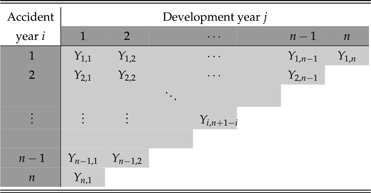
, are organized in a form of a right-angled isosceles triangle, as is the one shown in Table 1.
An example of the run-off triangle with the observed cumulative claim amounts
 $Y_{i,j}$
for
 $i = 1, \dots, n$
and
 $j = 1, \dots, n + 1 - i$
.

For a given run-off triangle, our task is to predict its “other half”: the yet unobserved random variables
 $Y_{i,j}$
on the (shorter and shorter) diagonals for
 $i = 2, \dots, n$
and
 $j = n - i +2, \dots, n$
. The interest of an insurance company lies particularly in the last column
 $\{Y_{i, n}\}_{i =2}^n$
, which represents the unknown ultimate cumulative amounts for the accident years
 $i =2, \dots, n$
. Sufficient funds have to be allocated to meet this end. The overall claims reserve is thus defined as
 $\sum_{i = 1}^{n} Y_{i, n}$
minus the amount already paid, the latter represented by the last observed diagonal. As this reserve consists of yet unobserved items, it has to be predicted. Beyond a mere point prediction, it is also important to predict (accounting for the uncertainty in the whole prediction process) the overall reserve distribution, to properly assess the reserving risk. A straightforward way to achieve this distribution are resampling methods like bootstrap.
In what follows, we briefly describe some traditional point prediction methods in claims reserving. The corresponding distributional predictions via bootstrap strategies are discussed in Section 5. All these methods are some variation or version of the chain ladder methodology. We use them for comparisons in Section 6.
2.1. Average development ratios
Basic building blocks in the chain ladder methodology are development ratios (factors). The stochastic underpinning of this methodology assumes that the cumulative claims
 $(Y_{i, 1}, \dots, Y_{i , n})$
are independent between the lines of the run-off triangle, accident years
 $i = 1,\dots, n$
. The “main assumption of the chain ladder stochastic model” (Mack, Reference Mack1993; Mack and Venter, Reference Mack and Venter2000)
 \begin{equation} \mathsf{E} \left[Y_{i, j + 1} | Y_{i, j}, \dots, Y_{i, 1}\right] = f_j Y_{i, j} \quad \mbox{for}\quad i = 1, \dots, n\quad \mbox{and}\quad j = 1, \dots, n-1,\end{equation}
is then postulated, introducing the development factors – unknown parameters
 $f_j$
’s. As (1) implicates that the
 $f_j$
’s do not depend on i, the Markov style assumption (1) complements the independence of rows by a “weak” identical distribution assumption – identical in terms of the moments involved in (1); everything is then also conditional on the initial values, the historical claim amounts from the same accident year. Since
 $\{Y_{i,j}\}_{j=1}^n$
are cumulative claim amounts, one can assume for certain claims triangles and the character of the loss data that
 $Y_{i,j+1}\geqslant Y_{i,j}$
almost surely for all i,j. Consequently, an additional restriction
 $f_j \geqslant 1$
could be imposed, which would create a submartingale structure on the underlying processes. The method described here estimates the unknown development factors
 $f_j$
as the average development ratios
 \begin{equation}\overline{f}_{j} = \frac{1}{n-j}\sum_{i=1}^{n-j} \hat{f}_{i,j} = \frac{1}{n-j}\sum_{i=1}^{n-j}\frac{Y_{i, j + 1}}{Y_{i, j}},\quad j=1,\ldots, n-1;\end{equation}
averaging over the specific development ratios
 $\hat{f}_{i,j}\,:\!=\,Y_{i,j+1}/Y_{i,j}$
.
The estimates of the parameters
 $f_j$
are used to predict the unobserved quantities in the run-off triangle: first, the immediately adjacent empty diagonal,
 \begin{equation}\widehat{\!Y}_{i,j} = \overline{f}_{j - 1} Y_{i, j - 1} \quad \mbox{for}\quad i = 2, \dots, n\quad \mbox{and}\quad j = n - i + 2,\end{equation}
and then the subsequent diagonals
 \begin{equation}\widehat{\!Y}_{i,j} = \overline{f}_{j - 1} \widehat{\!Y}_{i, j - 1} \quad \mbox{for}\quad i = 3, \dots, n\quad \mbox{and}\quad j \geqslant n - i + 3, \dots, n.\end{equation}
In the actuarial jargon, “the triangle is completed to a square,” a “squared triangle.” The overall predicted reserve is then obtained as
 \begin{equation}\mathscr{R} = \sum_{i = 2}^{n} \widehat{\!Y}_{i, n}- \sum_{i= 2}^{n} Y_{i, n+ 1-i}.\end{equation}
The reserving approach based on the averaged development ratios is straightforward, and the unknown distribution of
 $\mathscr{R}$
can be effectively resampled.
2.2. Volume-weighted average development ratios
The standard chain ladder approach to loss reserving modifies the previous method of estimating the development factors
 $f_j$
using volume-weighted average development ratios instead: each specific development factor
 $\hat{f}_{i,j}=Y_{i,j+1}/Y_{i,j}$
is weighted by the cumulative amount
 $Y_{i,j}$
from the same accident year and the same development year, resulting in the estimate
 \begin{equation}\breve{f}_j = \frac{\sum_{i = 1}^{n -j} Y_{i, j} \hat{f}_{i, j}}{\sum_{i = 1}^{n - j} Y_{i, j}} = \frac{\sum_{i = 1}^{n -j} Y_{i, j + 1}}{\sum_{i = 1}^{n - j} Y_{i, j}}\quad\mbox{for}\quad j = 1, \dots, n - 1.\end{equation}
The “completion of the square,” the predictions of claims reserves, and the overall reserve are then done analogously as in the previous method, that is, using the estimates (6) instead of (2) in prescriptions (3) and (4).
From the stochastic point of view, this approach is motivated, apart from the previously listed assumptions, by a specific assumption of Mack (Reference Mack1994, Reference Mack1999), which is further discussed in Section 4. From the practical point of view, Verdonck and Debruyne (Reference Verdonck and Debruyne2011) pointed out that the method of average development ratios may suffer from an undesirable sensitivity to certain atypical claim amounts; volume-weighted average development ratios may mitigate this. Early elaborations of the optimality for the estimators (2) and (6) within the autoregression framework were given by Kremer (Reference Kremer1984). Further investigations and comparisons can also be found in Mack and Venter (Reference Mack and Venter2000) or Hürlimann (Reference Hürlimann2009). For a broader overview, we refer to Taylor (Reference Taylor2000, Chapter 7). For more properties of both methods described above, see also Bühlmann (Reference Bühlmann1983), Wüthrich and Merz (Reference Wüthrich and Merz2008), and Pešta and Hudecová (Reference Pešta and Hudecová2012).
2.3. Overdispersed Poisson and gamma models
Other very common reserving methods are based on the overdispersed Poisson (ODP) and gamma models, which work in the framework of generalized linear models (McCullagh and Nelder, Reference McCullagh and Nelder1989). A distribution from the family of exponential dispersion models is assumed to be convenient for the incremental claims. In our setting, the run-off triangles are formed by the differences
 $X_{i,j} = Y_{i,j} - Y_{i,j-1}$
for all observed
 $Y_{i,j}$
(with the convention
 $Y_{i,0}\equiv 0$
). The expected values of
 $X_{i,j}$
are then assumed to follow the generalized linear model with the logarithmic link function
 \begin{equation}\log \left(\mathsf{E}\left[X_{i, j}\right]\right) = \gamma + \alpha_i + \beta_j,\end{equation}
where
 $\alpha_i \in \mathbb{R}$
relates to the accident year i and
 $\beta_j \in \mathbb{R}$
stands for the development period j;
 $\gamma \in\mathbb{R}$
is the intercept. For the sake of more flexibility regarding the volatility in the model, the overdispersion parameter
 $\phi > 0$
is introduced, modeling the variance of the incremental amounts:
 $\mathsf{Var}\,(X_{i,j}) = \phi\mu_{i,j}^{\delta}$
, where
 $\mu_{i,j}=\mathsf{E}(X_{i,j})$
and
 $\delta=1$
in the case of the ODP model, or
 $\delta=2$
in the case of the gamma model.
In the application part (Section 6), we focus on the ODP models not on the gamma models. Although it could look otherwise, it is well known (Mack and Venter, Reference Mack and Venter2000) that ODP yields the point predictions, which are identical to those obtained by the method of volume-weighted average development ratios. (In practice, a tiny difference can be sometimes observed, due to the different numerical algorithms used.) The latter mentioned method is nothing else than the standard chain ladder method reviewed in Section 2.2. There is one important detail, however: the equality of the predictions holds true only if ODP is able to yield any predictions at all. If some of the incremental claims are negative (which is not that uncommon in practice and may result from returned erroneous, fraudulent, or reimbursed claims), the methodology of generalized linear models fails to produce any result. The method of volume-weighted average development ratios delivers point predictions in any case. However, we still consider ODP a distinct method, because the different philosophy of the ODP approach results in a different way of obtaining the distributional predictions. The details are given in Section 5. For the sake of comparison, we compute point predictions by the ODP method via its definition (using generalized linear models) whenever possible (i.e., whenever all incremental claims are non-negative); otherwise, we use the chain ladder alternative.
3. The proposed methods
As mentioned in the introduction, the building block of all of the proposed methods is so-called functional development profiles, “patterns of loss emergence” (Clark, Reference Clark2003). The prediction of losses can be then seen as a completion, “reconstruction” (provided we were in the future when all predicted cumulative claim amounts are already known) of these profiles. To this end, however, we do not model them parametrically but rather seek how to do it in non-parametric ways.
3.1. Development profiles
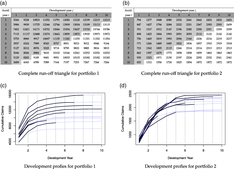
As an example, let us consider two different insurance portfolios with run-off triangles observed completely (which will occur at time
 $2n-1$
; in our examples
 $n=10$
). The squared triangles together with their observed and unobserved (“true reserves”) functional development profiles can be seen in Figure 1. At time n (indicated by the darker part of the tables), the solid lines represent the observed claims; dotted lines are the ones to be observed only in the future, not at time n. One run-off triangle (the top left panel) serves as a representative of the non-crossing and widely separated development profiles, whereas the other one (the top right panel) stands as a protagonist of the quite opposing group of run-off triangles, which have frequent crossings.
Complete “squared” run-off triangles for two different portfolios. Each curve corresponds to one row in the run-off triangle; solid lines are observed, dotted not observed run-off functional profiles for two representative portfolios.

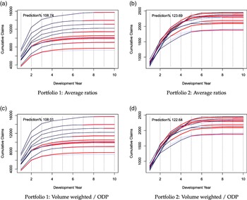
The predicted development profiles based on the observed run-off triangles (at time n) for the two parametric methods reviewed in Sections 2.1 and 2.2 are shown in Figure 2. The predictions are plotted in red; the prediction effectiveness – called Prediction% – is given in terms of the percentage ratio between the predicted reserve and the “true reserve.” The closer this value is to 100%, the better.
The prediction based on the average development ratios (top panels) and the volume-weighted development ratios (bottom panels). The two prediction approaches are similar for both portfolios. Under positive increments (which is all the case here), the ODP method is equivalent in point prediction to the volume-weighted average development ratios.

3.2. PARALLAX: Parallel approximation of missing fragments
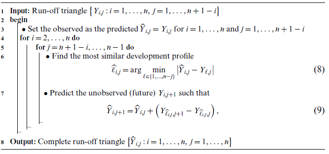
Two of the proposed methods are motivated by relatively straightforward graphical strategies. The first of them looks for the most similar development profile (in the
 $\ell^1$
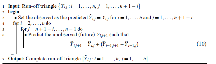
metric) among the profile fragments already observed. Such profile is then used to predict the future claims by adding it to the most recent claim (obtaining thus, in a sense, a parallel predicted profile), see Algorithm 1.
PARALLAX

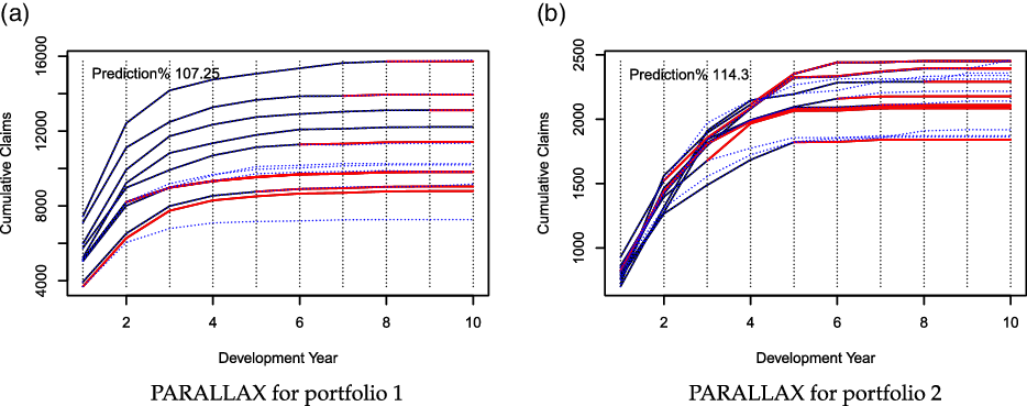
A preliminary comparison of the results of this algorithm applied to the run-off triangles from Figure 1 reveals that the algorithms appear to be more accurate than the standard methods, in terms of the overall reserve prediction. For the first triangle, the performance is pretty much similar (we achieve 107% of the true reserve compared to 109% or 108% given by the naïve average development ratio approaches). More evident difference occurs for the second triangle where both standard approaches overestimate the true reserve (giving 124% and 123%), while we predict the reserve slightly over 114%; see Figure 3. This can be perhaps explained by the fact that neither average development ratios nor the volume-weighted average development ratios can reflect the true underlying variability within the accident year specific development factors. Our algorithm instead seeks the most similar pattern within the observed loss development triangle, which then yields more accurate predictions.
The estimated functional profiles of the run-off triangles for two portfolios from Figure 1 using the parallel approximation PARALLAX. The reserve effectiveness is given as a percentage proportion of the estimated reserve and the true liability.

Of course, this is just a preliminary comparison concerning two haphazardly selected run-off triangles. A more complex comparison can be found in Section 6.
3.3. REACT: Approximation by the most recent accident year
The second proposed method can be viewed as a simplification of the first one. Its central principle is that regarding the future, the most relevant are the current and the previous year. The algorithm thus takes the development trend from the previous accident year and uses it to predict the next consecutive development, cf. Algorithm 2.
REACT

Obviously, the underlying principle of focusing on immediate rather than distant past may not be accepted universally. The fact that the algorithm seemingly “ignores” the earlier data may be interpreted as a drawback rather than virtue – especially if there is a strong belief in some stationary stochastic mechanism “generating” the data. On the other hand, the proponents of the principle may argue that the focus on recent data implicitly takes into account things like similar business strategy, company policy, client allocation, or comparative trading volumes (see, for instance, page 60 of Clark, Reference Clark2003). Such aspects, in particular, affect common portfolios where the overall trading volume follows some increasing/decreasing trend over the last years.
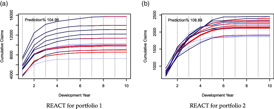
The preliminary comparison of the results visualized in Figure 4 shows now the prediction effectiveness of almost 105% and slightly less than 109% for the first and the second run-off triangles from Figure 1, respectively, that is, the algorithm outperforms not only the standard techniques but also our previous functional approach, PARALLAX. A more extensive comparison on other run-off triangles, however, suggests that while there are portfolios that are more appropriate for the parallel approximation, PARALLAX (those with more volatile claims and unstable developments – side effects of natural disasters, etc.), there are also portfolios depending on the most recent accident year (for instance, portfolios with some significant trend in the incurred claims over the last years) – for which REACT scores instead.
The estimated functional profiles of the run-off triangles for two portfolios from Figure 1 using the most recent accident year approximation REACT. The reserve effectiveness is given as a percentage proportion of the estimated reserve and the true liability.

3.4. MACRAME: Markov chain fragment approximation
Working on the previous methods in the actuarial context, we came across similar ideas treated from a different perspective, that of statistical techniques for partially observed functional data. In the context of functional data with observation missing at random, Delaigle and Hall (Reference Delaigle and Hall2013) used a similar graphical representation and proposed methods analogous to ours.
While our situation differs from theirs, because the pattern of missingness in our triangular data is not random but deterministic (structured and fully determined by the underlying actuarial nature), the follow-up ideas of Delaigle and Hall (Reference Delaigle and Hall2016), who estimated the missing functional fragments within a Markov chain and then used the estimated transition probabilities to complete the unobserved parts, inspired the extension of our methodology, also via Markov chain approach. It may be of some interest that these connections are putting our efforts somewhat in the context of statistical functional data analysis – although it should be noted that the latter area is otherwise vast, and thus beyond our ambitions to cover here. In the actuarial literature, the idea of the Markov chain for the claims reserving problems was considered, in the context of granular data, by Hesselager (Reference Hesselager1994).
Our third algorithm is thus based on viewing the lines of the run-off triangles as specific finite Markov chains. In this vein, it first forms another, same-size run-off triangle
 $\{U_{i, j}\}$
, which should mimic the original incremental run-off triangle
 $\{X_{i,j}\}$
and whose entries are all in the same finite set
 $\mathscr{S}$
corresponding to a grid
 $-\infty = g_0 \leqslant g_1 \leqslant \dots \leqslant g_{m-1} \leqslant g_m=+\infty$
. The details about how
 $\mathscr{S}$
is determined are discussed below. The values
 $U_{i,j}$
’s, which are assigned to be some
 $u_k\in[g_{k-1},g_k)$
if
 $g_{k-1}<g_k$
and
 $X_{i,j}\in[g_{k-1},g_k)$
, are then assumed to behave as the outcomes of a homogeneous Markov chain with state space
 $\mathscr{S}$
, with the same distribution for every i-th line (every accident year) in the triangle. This means, in particular, that the transition probabilities
 $p(s_1,s_2)=\mathsf{P}[U_{i, j + 1} = s_2|U_{i, j}= s_1]$
are the same for all i,j and for any
 $s_1,s_2\in\mathscr{S}$
. They can thus be estimated by the ratio
 \begin{equation} \widehat{p}(s_1, s_2) = \frac{\displaystyle\sum_{j=1}^{n-1} \frac{1}{n-j} \sum_{i=1}^{n-j} \unicode{x1D7D9}{\left\{ U_{i, j} = s_1, U_{i, j + 1} = s_2\right\}} } {\displaystyle \sum_{j=1}^{n-1} \frac{1}{n-j} \sum_{i=1}^{n-j} \unicode{x1D7D9}{\left\{ U_{i, j} = s_1\right\}} },\end{equation}
where
 $\unicode{x1D7D9}\{\cdot\}$
is the indicator function, and they form the estimated transition probability matrix
 $\widehat{\mathbb{P}}=\{\widehat{p}_{\ell_1,\ell_2}\}_{\ell_1=1,\ell_2=1}^{|\mathscr{S}|,|\mathscr{S}|}\in\mathbb{R}^{|\mathscr{S}|\times|\mathscr{S}|}$
, where
 $\widehat{p}_{\ell_1,\ell_2}=\widehat{p}\left(\mathscr{S}_{(\ell_1)},\mathscr{S}_{(\ell_2)}\right)$
and
 $\mathscr{S}_{(\ell)}$
is the
 $\ell$
-th smallest element of
 $\mathscr{S}$
. However, for the run-off triangles with extremely short developments (e.g., fully developed profiles in the second or third development period with mostly zero increments), it may be convenient to exaggerate the state in which the run-off triangle is already fully developed. For this purpose, we propose to use a transition probability matrix being defined as a convex combination
 \begin{equation}\widetilde{\mathbb{P}}\,:\!=\,(1-\delta_n)\widehat{\mathbb{P}}+\delta_n\mathbb{I}_0,\end{equation}
of the original matrix
 $\widehat{\mathbb{P}}$
and an additional exaggeration matrix
 $\mathbb{I}_0$
, which is either a stochastic matrix with the column corresponding to the state
 $0\in\mathscr{S}$
consisting of all ones and the remaining entries are zero if
 $0\in\mathscr{S}$
, or it is a zero matrix otherwise, that is,
 $\mathbb{I}_0\,:\!=\,\{\iota_{\ell_1,\ell_2}\}_{\ell_1=1,\ell_2=1}^{|\mathscr{S}|,|\mathscr{S}|}\in\mathbb{R}^{|\mathscr{S}|\times|\mathscr{S}|}$
and
 $\iota_{\ell_1,\ell_2}=\unicode{x1D7D9}\{\mathscr{S}_{(\ell_2)}=0\}$
. The mixing coefficient from (12) is defined as
 \begin{equation*}\delta_n\,:\!=\,\begin{cases}\frac{1}{n}\sum_{s\in\mathscr{S}}\widehat{p}(s,0), & 0\in \mathscr{S};\\[4pt]0, & 0\notin \mathscr{S}.\\\end{cases}\end{equation*}
Note that for the triangles with not fully developed pay-off profiles, it holds that
 $\delta_n=0$
and, thus, the original transition probability matrix
 $\widehat{\mathbb{P}}$
is used.
The estimated transition probabilities
 $\widetilde{p}(s_1,s_2)$
(i.e., the elements of
 $\widetilde{\mathbb{P}}$
) are then utilized to predict the values of the original incremental run-off triangle
 $\{X_{i, j}\}$
from the current “diagonal” state
 $U_{i,n+1-i}$
,
 $i=2,\ldots,n$
, through the (conditional) expected value
 \begin{equation}\widehat{X}_{i,n+2-i} = \sum_{\ell=1}^{|\mathscr{S}|} \widetilde{p}\left(U_{i,n+1-i},s_{\ell}\right)s_{\ell},\quad i=2,\ldots,n.\end{equation}
The predictions of the further missing states of the “converted” run-off triangle
 $\{U_{i, j}\}$
(from the original triangle
 $\{X_{i,j}\}$
) are then obtained through the Markov property as
 \begin{align*}\widehat{X}_{i,n+1-i+h} & = \sum_{\ell_1=1}^{|\mathscr{S}|}\sum_{\ell_2=1}^{|\mathscr{S}|}\ldots\sum_{\ell_h=1}^{|\mathscr{S}|}\widetilde{p}\left(U_{i,n+1-i},s_{\ell_1}\right)\widetilde{p}\left(s_{\ell_1},s_{\ell_2}\right)\ldots\widetilde{p}\left(s_{\ell_{h-1}},s_{\ell_h}\right)s_{\ell_h},\\& \qquad\qquad\qquad\qquad\qquad\qquad\qquad\qquad 2\leqslant h<i\leqslant n.\end{align*}
The tenability of treating the lines of the converted triangle
 $\{U_{i,j}\}$
as Markov chains is supported in the chain ladder context by the widely accepted “main assumption of the chain ladder model” (1) – which implies
 $\mathsf{E}[X_{i,j+1}|X_{i,j},\ldots,X_{i,1}]=(f_j-1)\sum_{k=1}^jX_{i,k}$
and is, as was already remarked, a sort of “Markov property for moments.” Also, as the
 $U_{i,j}$
’s are (deterministic) functions of the
 $X_{i,j}$
’s, the independence and the Markov properties formulated for the latter are inherited by the former. The only objection here may be raised against the homogeneity of the underlying Markov chains. Indeed, the
 $f_j$
’s in (1) are not considered equal for different j. However, one should keep in mind that the transition probabilities of the pertinent Markov chains are more elaborate structure than the simple multipliers
 $f_j$
’s. Due to the generally row-wise decreasing nature of the incremental amounts, different transition probabilities are likely to apply in later than in the earlier stages of claims development (so assuming that the whole transition matrix remains the same does not result in much loss of generality).
Considering originally the general Markov model in a general situation, without assuming homogeneity, we realized that the stochastic theory would deliver desired conclusions, once consistent estimates of the transition probabilities are available. That turned out, however, to be a problem: the general situation admits too many transition probabilities, too many unknown parameters; the subsequent estimates depend effectively on very few observations and are inevitable too volatile. While these obstacles could be perhaps overcome by alternative estimation scenarios like compound estimation (estimating transition probabilities from a group of run-off triangles with similar characteristics), or by stabilizing the estimates via using a priori expert information, we defer these alternatives rather to future research and, at this point, we adopt the homogeneity assumption – if perhaps only as an approximation rather than a faithful reflection of reality. In fact, the conversion of the continuous setting to Markov chain on finite number of states is yet another approximation aspect here. Treating the underlying Markov chains as homogeneous turned out to be a crucial stabilizing component – not only regarding the estimates but also leading to better predictions.
The usual estimators of transition probabilities in Markov chain models are the intuitive ones, coming up as maximum likelihood estimators: a transition probability is estimated by the simple ratio of observed transitions under question to all transitions observed from the particular state. Under the homogeneity assumption, the numerator and the denominator are aggregated over the whole observed Markov chain. A close inspection of (11) reveals that the estimators defined there are slightly different: they include an additional weighing term
 $1/(n-j)$
, both in the numerator and the denominator. Intuitively, this term is connected to the number of observations in the j-th column of a run-off triangle. The deeper reasons for its inclusion follow from Theorem 5 which shows that such a modification is necessary in our specific setting of missing observations in a run-off triangle: to obtain estimators of transition probabilities that are consistent.
While the scheme of the MACRAME Algorithm 3 remains the same for any selection of the Markov states, the choice of the grid points
 $-\infty = g_0 \leqslant g_1 \leqslant \dots \leqslant g_{m-1} \leqslant g_m=+\infty$
, this technical detail may be important in practical applications. While it is convenient to have as many states as possible (for the sake of the fine approximation of the true development process), the size of the data available to estimate the transition probabilities prevents the number of states from becoming too large. We found the following guidelines helpful:
-
(i) in order to have the 1–1 transformation effect both in time and the incremental amounts, the number of grid points should be the same as the number of the development periods,
 $m = n$
;
-
(ii) the incremental values excluding the first column
$\{x_{(i+j-3)(i+j-2)/2+i}\,:\!=\,X_{i,j}\,:\,j>1;\,i+j\leqslant n+1\}$
are ordered and equidistantly split into m intervals according to the grid points
\begin{equation*}g_k\,:\!=\,x_{\left(\left\lceil \frac{kn(n-1)}{2m}\right\rceil+1\right)},\quad k=1,\ldots,m-1;\end{equation*}
-
(iii) the states are medians of the incremental values belonging to these intervals, i.e.,
where median of an empty set is omitted.
\begin{equation*}\mathscr{S}\,:\!=\left\{u_k\,:\!=\,\mbox{median}\!\left(X_{i,j}\in[g_{k-1},g_k)\,:\,j>1,i+j\leqslant n+1\right)\!,\,k=1,\ldots,m\right\}\!,\end{equation*}


Note that some of the intervals
 $[g_{k-1},g_k)$
can be empty sets, because several
 $X_{i,j}$
’s can have the same value, and therefore
 $t\,:\!=\,|\mathscr{S}|\leqslant m$
. The above stated procedure is completely data-driven, where neither nuisance parameters nor tuning constants are involved. Consequently, we assign the obtained value
 $u_k$
as the realization of the Markov process
 $\{U_{i,j}\}_j$
such that
 $U_{i,j}\,:\!=\,u_k$
when
 $X_{i,j}\in[g_{k-1},g_k)$
.
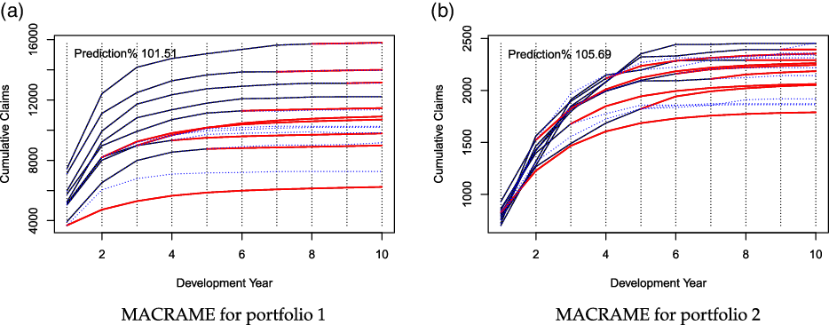
There are, obviously, many different ways to tackle the states’ selection: different interval lengths can be used, more states can be defined – all this constitutes additional topics for further investigation. For instance, a kind of expert judgment can also intervene here: if there is a reasonable belief or conviction about the shape of the curves representing the incremental profiles (based on historical observations or long-term knowledge), the intervals (and, hence, states) can be then constructed accordingly. Nonetheless, we used the above formulated choice of the Markov states in our implementation (Algorithm 3) – which was then applied again to the two portfolios from Figure 1. The prediction effectiveness achieves
 $101.5\%$
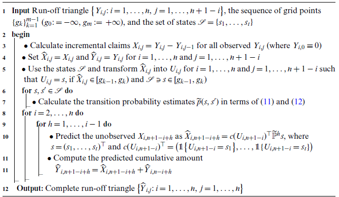
for the first portfolio and slightly less than 106% for the second one (Figure 5) – which is the best result so far: not only surpasses our first two methods but beats the standard ones as well. On the top of that, the more extensive analysis in Section 6 reveals that MACRAME may also have its merits for less typical run-off triangles.
MACRAME

The estimated functional profiles of the run-off triangles for two portfolios from Figure 1 using the Markov chain reserving method MACRAME. The reserve effectiveness is given as a percentage proportion of the estimated reserve and the true liability.

4. Rigorous results in theoretical setting
As indicated in the introduction, the proposed methods apply to all kinds of loss development triangular data and require no formal assumptions. Nonetheless, their favorable behavior in certain tractable stochastic situations may reinforce the belief in their effectiveness. In other words, if they behave well in certain ideal circumstances, there is a hope that they would behave well also in less ideal ones.
This section provides some results in this line of inquiry. Hereafter, all cumulative claim amounts
 $Y_{i,j}$
’s are thus considered to be random variables on a probability space
 $(\Omega,\mathscr{F},\mathsf{P})$
for all
 $i,j\in\mathbb{N}$
.
The standing assumption for all methods, inherited from the chain ladder methodology, is the assumption of independence. It means that the processes of cumulative claim amounts corresponding to a different accident (origin) period are independent, because claims from different accident periods are naturally considered as independent. The validity and limitations of this assumption have been a subject of numerous discussions. Notwithstanding, it is a cornerstone of pretty much every theoretical analysis of claims reserving techniques.
Assumption I. The processes
 $\{Y_{i, j}\}_{j\in\mathbb{N}}$
are independent for all
 $i\in\mathbb{N}$
.
The following assumption incorporates the already discussed “main assumption” (1), together with the assumption regarding variance, also standard in the chain ladder theory (Mack, Reference Mack1993).
Assumption C. For all
 $i,j\in\mathbb{N}$
,
 $\mathsf{E}\!\left[Y_{i,j+1}|Y_{i,j},\ldots,Y_{i,1}\right]=f_jY_{i,j}$
and
 $\mathsf{Var}\!\left[Y_{i,j+1}|Y_{i,j},\ldots,Y_{i,1}\right]=\sigma_j^2Y_{i,j}$
, where
 $f_j>0$
and
 $\sigma_j^2>0$
.
The stochastic consistency of the proposed methods will be formulated and proved in terms of conditional convergence in mean square in probability. We refer to Belyaev (Reference Belyaev1995) for more details. Suppose that Z is a random variable,
 $\{Z_n\}_{n=1}^{\infty}$
is a sequences of random variables,
 $\boldsymbol{W}$
is a set of random variables, and
 $\{\boldsymbol{W}_n\}_{n=1}^{\infty}$
is a sequence of sets of random variables. All the random entities have finite mean on a probability space
 $(\Omega,\mathscr{F},\mathsf{P})$
. The conditional probability given some
 $\boldsymbol{W}$
is defined as
 $\mathsf{P}_{\boldsymbol{W}}[\cdot]\,:\!=\,\mathsf{E}_{\mathsf{P}}[\unicode{x1D7D9}({\cdot})|\boldsymbol{W}]$
, where
 $\unicode{x1D7D9}({\cdot})$
is the indicator function. The conditional expectation given some
 $\boldsymbol{W}$
then corresponds to
 $\mathsf{E}_{\boldsymbol{W}}[\cdot]\equiv\mathsf{E}_{\mathsf{P}}[\cdot|\boldsymbol{W}]$
.
Definition 1 (Conditional convergence in
 $\mathsf{L}_p$
in probability). For
 $p\geqslant 1$
, to say that
 $Z_n$
converges to Z in
 $\mathsf{L}_p(\boldsymbol{W}_n)$
as n tends to infinity in probability
 $\mathsf{P}$
, i.e.,
 $Z_n\xrightarrow[n\to\infty]{\mathsf{L}_p(\boldsymbol{W}_n)}Z$
in probability
 $\mathsf{P}$
, means
 \begin{equation*}\forall\epsilon>0\,:\,\lim_{n\to\infty}\mathsf{P}\left[\mathsf{E}_{\boldsymbol{W}_n}\left|Z_n-Z\right|^p>\epsilon\right]=0.\end{equation*}
Let
 $T_{i,j}^{(n)}=\{Y_{k,\ell}\,:\,k\leqslant i,\,\ell\leqslant j,\,k+\ell\leqslant n+1\}$
, be a “cut triangle,” a part of the observed run-off triangle with the calendar period less than or equal to
 $n+1$
containing the cumulative claim amounts up to the i-th accidental and j-th development period only. Note that
 $\{Y_{i,1},\ldots,Y_{i,j}\}\subset T_{i,j}^{(n)}$
for every
 $i+j\leqslant n+1$
. Under Assumptions I and C, the chain ladder method provides unbiased estimators of the development factors
 $f_j$
in the form of
 \begin{equation} \breve{f}_j^{(n)} =\frac{\sum_{i = 1}^{n -j} Y_{i, j + 1}}{\sum_{i = 1}^{n - j} Y_{i, j}}.\end{equation}
The conditional mean square error of the chain ladder estimator then becomes
 \begin{equation}\mathsf{E}\bigg[\Big\{\breve{f}_j^{(n)}-f_j\Big\}^2\Big|T_{n+1-j,j}^{(n)}\bigg]=\mathsf{Var}\,_{T_{n+1-j,j}^{(n)}}\breve{f}_j^{(n)}=\frac{\sigma_j^2}{\sum_{i = 1}^{n - j} Y_{i, j}}\quad [\mathsf{P}]\mbox{-a.s.},\end{equation}
which in turn establishes the conditional convergence in means square for the chain ladder method when
 $\sum_{i=1}^{n-j} Y_{i,j}\to\infty$
 $[\mathsf{P}]$
-a.s. as
 $n\to\infty$
(Pešta and Hudecová, Reference Pešta and Hudecová2012).
4.1. PARALLAX
The following assumption expresses stochastic stability for the cumulative claim amounts from the same development period after several (n) observation (calendar) periods. For the PARALLAX algorithm, it is analogous to the assumption for the chain ladder method requiring that
 $\sum_{i=1}^{n-j}Y_{i,j}\to\infty$
 $[\mathsf{P}]$
-a.s. as
 $n\to\infty$
for every
 $j\in\mathbb{N}$
. It is an “internal consistency criterion” which in turn implies stochastic consistency, consistency in terms of the convergence of
 $\breve{f}_j^{(n)}$
in the chain ladder methodology – Pešta and Hudecová (Reference Pešta and Hudecová2012) showed that it is in fact necessary and sufficient there.
Assumption P.
 $\frac{Y_{\widehat{\ell}_{n+\kappa-j,j},j}}{\mathsf{E}\left\{Y_{n+\kappa-j,j}\big|T_{n+\kappa-j,j-\kappa+1}^{(n)}\right\}}\xrightarrow[n\to\infty]{\mathsf{P}}1$
and
 $\frac{Y_{\widehat{\ell}_{n+\kappa-j,j},j}^{1/2}}{\mathsf{E}\left\{Y_{n+\kappa-j,j}\big|T_{n+\kappa-j,j-\kappa+1}^{(n)}\right\}}\xrightarrow[n\to\infty]{\mathsf{P}}0$
for all
 $j,\kappa\in\mathbb{N}$
.
This assumption states that the closest observed value
 $Y_{\widehat{\ell}_{n+\kappa-j,j},j}$
from the historical data
 $Y_{1,j},\ldots,Y_{n-j,j}$
for the j-th development period to the cumulative claim amount
 $Y_{n+\kappa-j,j}$
has to be close to the conditional expectation of
 $Y_{n+\kappa-j,j}$
(given the observed data) in the sense that their ratio tends to one in probability. Basically, it reflects a belief that there exists some historical value, which resembles the unknown one that is going to be used for predicting the consecutive cumulative row amount
 $Y_{n+\kappa-j,j+1}$
. Furthermore, the square root of the closest historical cell is naturally negligible in probability to the conditional expectation of the value that is going to be involved in prediction of the consecutive
 $Y_{n+\kappa-j,j+1}$
. For
 $\kappa=1$
, Assumption P reduces to
 $Y_{\widehat{\ell}_{n+1-j,j},j}/Y_{n+1-j,j}\xrightarrow[n\to\infty]{\mathsf{P}}1$
and
 $Y_{\widehat{\ell}_{n+1-j,j},j}/Y_{n+1-j,j}^2\xrightarrow[n\to\infty]{\mathsf{P}}0$
for all
 $j\in\mathbb{N}$
, because
 $Y_{n+1-j,j}\in\sigma\Big(T_{n+1-j,j}^{(n)}\Big)$
, where
 $\sigma({\cdot})$
stands for the corresponding
 $\sigma$
-algebra.
For the PARALLAX algorithm now, the estimator of the chain ladder development factor
 $f_{j}$
becomes row specific
 \begin{equation}\widehat{f}_{i,j}^{(n)}\,:\!=\,1+\frac{Y_{\widehat{\ell}_{i,j},j+1}-Y_{\widehat{\ell}_{i,j},j}}{\widehat{\!Y}_{i,j}}\end{equation}
for
 $i+j\geqslant n+1$
, if
 $\widehat{\!Y}_{i,j}\neq 0$
; otherwise it is set to one. Essentially, the estimator
 $\widehat{f}_{i,j}^{(n)}$
is calculated from a trapezoid
 \begin{equation*}\left\{Y_{k,\ell}\,:\,1\leqslant k\leqslant i,\,n+1-i\leqslant \ell\leqslant j+1,\,k+\ell\leqslant n+1\right\}=T_{i,j+1}^{(n)}\setminus T_{i,n-i}^{(n)}\subset T_{i,j+1}^{(n)},\end{equation*}
whereas the traditional chain ladder estimator
 $\breve{f}_j^{(n)}$
is computed only from the two-column rectangle
 $\{Y_{k,\ell}\}_{k=1,\ell=j}^{n-j,j+1}\subset\mathbb{R}^{(n-j)\times 2}$
. This means that more data entries are always involved in every prediction step of the PARALLAX technique compared to the chain ladder, which makes the PARALLAX more adaptive to the input data. In the following theorem, the consistency of the PARALLAX method, together with the related conditional mean square error, is established. The result is analogous to that for the chain ladder method reviewed in the preamble of Section 4.
Theorem 1. Under Assumptions I, C, and P,
 \begin{equation*}\widehat{f}_{i,j}^{(n)}\xrightarrow[n\to\infty]{\mathsf{L}_2\big(T_{i,j}^{(n)}\big)}f_j,\end{equation*}
in probability
 $\mathsf{P}$
for any
 $j\in\mathbb{N}$
such that
 $i=n+\kappa-j$
, where
 $\kappa\in\mathbb{N}$
is a fixed constant. The conditional mean square error of the PARALLAX estimator of
 $f_j$
is
 \begin{equation*}\mathsf{E}\bigg[\Big\{\widehat{f}_{i,j}^{(n)}-f_j\Big\}^2\Big|T_{i,j}^{(n)}\bigg]=\frac{\sigma_j^2Y_{\widehat{\ell}_{i,j},j}}{Y_{n+1-j,j}^2}+(f_j-1)^2\Bigg(\frac{Y_{\widehat{\ell}_{i,j},j}}{Y_{n+1-j,j}}-1\Bigg)^2\quad [\mathsf{P}]\mbox{-a.s.},\end{equation*}
when
 $\kappa=1$
, and, for
 $\kappa>1$
, it becomes
 \begin{align*}\mathsf{E}\bigg[\Big\{\widehat{f}_{i,j}^{(n)}-f_j\Big\}^2\Big|T_{i,j}^{(n)}\bigg] = & \frac{\sigma_j^2Y_{\widehat{\ell}_{i,j},j}}{Y_{i,n+1-i}^2\prod_{k=n+1-i}^{j-1}\left\{\widehat{f}_{i,k}^{(n)}\right\}^2}\\[5pt]& +(f_j-1)^2\Bigg\{\frac{Y_{\widehat{\ell}_{i,j},j}}{Y_{i,n+1-i}\prod_{k=n+1-i}^{j-1}\widehat{f}_{i,k}^{(n)}}-1\Bigg\}^2\quad [\mathsf{P}]\mbox{-a.s.}\end{align*}
Considering the search for the most similar development profile in (8), the following approximations become feasible
 \begin{equation*}\frac{Y_{\widehat{\ell}_{i,j},j}}{Y_{n+1-j,j}}\approx 1\quad\mbox{and}\quad\frac{\sigma_j^2Y_{\widehat{\ell}_{i,j},j}}{Y_{n+1-j,j}^2}\approx\frac{\sigma_j^2}{Y_{n+1-j,j}}.\end{equation*}
Hence, the conditional mean square error of the PARALLAX development factors’ estimators can be approximated by
 \begin{equation*}\mathsf{E}\bigg[\Big\{\widehat{f}_{n+1-j,j}^{(n)}-f_j\Big\}^2\Big|T_{n+1-j,j}^{(n)}\bigg]\approx\frac{\sigma_j^2}{Y_{n+1-j,j}},\end{equation*}
which in many practical cases will be greater than the conditional mean square error of the chain ladder development factors’ estimators (15), since we usually have
 $Y_{n+1-j,j}<\sum_{i = 1}^{n - j} Y_{i, j}$
 $[\mathsf{P}]$
-almost surely. Nonetheless, the PARALLAX estimators differ for every row i, which brings additional adaptability and causes that the conditional mean square errors of the PARALLAX and the chain ladder estimators are not directly comparable.
The claims triangle growing height-wise can be considered merely a technical affirmation. If it is desired to keep the size of the triangle fixed, one can deal with convergence in terms of an exposure measure. Based on the underlying individual claim dynamics, it is natural to explicitly introduce the accident year specific exposures
 $n_i$
that corresponds to the number of contracts or the number of claims for the accident year i (Verrall et al., Reference Verrall, Nielsen and Jessen2010; Huang et al., Reference Huang, Qiu and Wu2015, Reference Huang, Wu and Zhou2016; Wahl et al., Reference Wahl, Lindholm and Verrall2019). Suppose that every
 $Y_{i,j}$
can be decomposed as a random sum having
 $N_{i,j}$
summands of the independent and identically distributed individual payments
 $\left\{C_{i,j,k}\right\}_k$
, i.e.,
 $Y_{i,j}=\sum_{k=1}^{N_{i,j}}C_{i,j,k}$
. If
 $N_{i,j}$
’s have the same expectation for all j’s, then Wald’s first equality yields
 $\mathsf{E} Y_{i,j}=\mathsf{E} N_{i,1}\mathsf{E} C_{i,j,1}$
. The following assumption incorporates such a property.
Assumption E.
 $\mathsf{E} Y_{i,j}=n_i\eta_j$
for all
 $i,j\in\mathbb{N}$
.
The reason for considering the parameter
 $\eta_j$
being independent of i comes from the chain ladder Assumption C, which implies
 $f_j=\mathsf{E} Y_{i,j+1}/\mathsf{E} Y_{i,j}$
(due to the tower property) and it is supposed that the development factor
 $f_j$
itself is independent of i. Hence,
 $f_j=\eta_{j+1}/\eta_j$
.
The consequent consistency result provides a large-exposure approximation, where the asymptotics is not in the dimension of the claims triangle (n), but in the volume of its cells.
Theorem 2. Under Assumptions I, C, and E, for any
 $j\in\{1,\ldots,n-1\}$
and
 $i\in\{n+1-j,\ldots,n\}$
,
 \begin{equation*}\widehat{f}_{i,j}^{(n)}\xrightarrow[n_i\to\infty]{\mathsf{P}}f_j,\end{equation*}
if
 $n_i/n_1\to 1$
and
 $\mathsf{Var}\, Y_{i,1}/n_i^2\to 0$
as
 $n_i\to\infty$
for every
 $i\in\{1,\ldots,n\}$
.
This theorem can be even extended by assuming that the row-wise volumes in the claims triangle tend to some constant different from one, that is,
 $n_i/n_1\to \nu_i\neq 1$
. Nevertheless, an estimator of
 $\nu_i$
is then required, which brings additional technical issues, cf. Huang et al. (Reference Huang, Qiu and Wu2015).
Moreover, an assumption on the variance of the first column’s elements
 $Y_{i,1}$
’s is needed in Theorem 2, because the standard chain ladder assumption C is postulated in a telescopic manner, and it does not provide information about the row-wise initial
 $\mathsf{Var}\, Y_{i,1}$
. Note that the assumption on
 $\mathsf{Var}\, Y_{i,1}$
is implied by Wald’s second inequality
 $\mathsf{Var}\, Y_{i,1}=\mathsf{Var}\, N_{i,1}(\mathsf{E} C_{i,1,1})^2+\mathsf{E} N_{i,1}\mathsf{Var}\, C_{i,1,1}$
and the assumption
 $\mathsf{Var}\, N_{i,1}=const\times \mathsf{E} N_{i,1}$
proposed in, for instance, Verrall et al. (Reference Verrall, Nielsen and Jessen2010), Huang et al. (Reference Huang, Qiu and Wu2015), Huang et al. (Reference Huang, Wu and Zhou2016), or Wahl et al. (Reference Wahl, Lindholm and Verrall2019).
4.2. REACT
For REACT, Assumption P is replaced by the following Assumption R, expressing again a type of stochastic stability between two consecutive cumulative claim amounts from the same development period after several (n) observation periods are given.
Assumption R.
 $Y_{n-j,j}/Y_{n+1-j,j}\xrightarrow[n\to\infty]{\mathsf{P}}1$
and
 $Y_{n-j,j}/Y_{n+1-j,j}^2\xrightarrow[n\to\infty]{\mathsf{P}}0$
for all
 $j\in\mathbb{N}$
.
This assumption indicates that within the same j-the development year the current value
 $Y_{n+1-j,j}$
and the previous one
 $Y_{n-j,j}$
are getting closer in probability as the size of the claims triangle increases. Moreover, the second part of the assumption reflects that
 $Y_{n-j,j}$
is naturally negligible compared to
 $Y_{n+1-j,j}^2$
. From a practical point of view, if there is some known claims inflation present in the run-off triangle, it should be removed by deflating the claim amounts accordingly (e.g., Verrall et al., Reference Verrall, Nielsen and Jessen2010, Section 6) in order to fulfill this assumption.
The REACT estimator of the chain ladder development factor is defined as
 \begin{equation}\widetilde{f}_j^{(n)}\,:\!=\,1+\frac{Y_{n-j,j+1}-Y_{n-j,j}}{Y_{n+1-j,j}}\end{equation}
if
 $Y_{n+1-j,j}\neq 0$
, otherwise is equal to one. The chain ladder development factors’ estimators are linearly defined, since they are (weighted) least squares estimates within the Aitken heteroscedastic linear regression model (Murphy, Reference Murphy1994). And, thus, unbiasedness comes hand in hand with linearity. Since our estimators (from PARALLAX as well as from REACT) of the development factors are clearly not linearly defined, it cannot be expected that they would be unbiased. Nonetheless, being consistent should be viewed as a desirable property for a suitable estimator. The following theorem presents the similar type of result for the REACT as Theorem 1 for the PARALLAX.
Theorem 3. Under Assumptions I, C, and R,
 \begin{equation*}\widetilde{f}_j^{(n)}\xrightarrow[n\to\infty]{\mathsf{L}_2\big(T_{n+1-j,j}^{(n)}\big)}f_j,\end{equation*}
in probability
 $\mathsf{P}$
for any
 $j\in\mathbb{N}$
. The conditional mean square error of the REACT estimator of
 $f_j$
is
 \begin{equation*}\mathsf{E}\bigg[\Big\{\widetilde{f}_j^{(n)}-f_j\Big\}^2\Big|T_{n+1-j,j}^{(n)}\bigg]=\frac{\sigma_j^2Y_{n-j,j}}{Y_{n+1-j,j}^2}+(f_j-1)^2\Bigg(\frac{Y_{n-j,j}}{Y_{n+1-j,j}}-1\Bigg)^2\quad [\mathsf{P}]\mbox{-a.s.}\end{equation*}
The latter theorem asymptotically reproduces the regular chain ladder when the claims triangle growing height-wise. The next consistency result is again as Theorem 2 in terms of an exposure measure, while keeping the size of the triangle fixed.


4.3. MACRAME
The independence of the processes
 $\{U_{i,j}\}_{j\in\mathbb{N}}$
for all rows of the converted incremental run-off triangle follows immediately by Assumption I from the independence of the processes in the rows of the original cumulative run-off triangle
 $\{\!Y_{i,j}\}$
. While the analogous implication would hold in the same direction for the Markov property, it is more expedient to formulate the following assumption, central for the stochastic behavior of the MACRAME, directly in terms of the “converted” triangle
 $\{U_{i,j}\}$
.
Assumption M. For every
 $i\in\mathbb{N}$
, the process
 $\{U_{i,j}\}_{j\in\mathbb{N}}$
is a homogeneous Markov chain with the transition probabilities
 $p(s_1, s_2) = \mathsf{P}[U_{i, j + 1} = s_2 | U_{i, j} = s_1]$
for every j and any
 $s_1,s_2\in\mathscr{S}$
.
The assumption of a homogeneous Markov chain has already been motivated in Subsection 3.4. Note that the chain ladder assumption of proportionality of the consequent incremental claim amounts for the same origin period
 $\mathsf{E} [X_{i, j + 1}|X_{i, j},\ldots,X_{i, 1}]=(f_j-1)\sum_{k=1}^jX_{i,k}$
is not contradicted here. By Assumption M,
 \begin{equation}\mathsf{E} [U_{i, j + 1}|U_{i, j},\ldots,U_{i, 1}]=\sum_{s\in\mathscr{S}}s p(U_{i, j},s)\quad \mbox{for all }i,j.\end{equation}
Despite the homogeneity of the assumed Markov chains, formula (18) for the incremental claim amounts is a non-homogeneous one; the right-hand side of (18) depends on j. Therefore, in terms of the traditional chain ladder model, the model implied by Assumption M can be considered as competitive. Note also that there is no finite variance assumption on the original
 $X_{i,j}$
’s. Thus, another theoretical advantage of the MACRAME method is that it is suitable also for heavy-tailed distributions.
The following assumption, which may be considered as a stabilizing or stationarity condition, is also more expediently formulated in terms of the converted run-off triangle. It basically ensures that there is sufficient number of data entries in the incremental run-off triangle for each state of the Markov chain. In case of the proposed guideline (i)–(iii) from Subsection 3.4 for defining the states, this assumption is automatically satisfied.
Assumption B. For any
 $s\in\mathscr{S}$
, the sequence
 $\big\{\frac{1}{n}\sum_{j=1}^{n-1}\frac{1}{n-j}\sum_{i=1}^{n-j}\mathsf{P}[U_{i, j} = s]\big\}_{n\in\mathbb{N}}$
is bounded away from zero.
The MACRAME method is characterized through the transition probabilities, which can be regarded as unknown parameters. Its coherence and usability thus follow from the consistency result of the following theorem, expressed via stochastic representation.
Theorem 5. Under Assumptions I, M, and B,
 \begin{equation*}\widetilde{p}(s_1, s_2) = p(s_1, s_2) + \mathscr{O}_{\mathsf{P}}\left(n^{-1/2}\right),\ n\to\infty,\end{equation*}
for every
 $s_1,s_2\in\mathscr{S}$
.
In order to provide a finite sample justification for a fixed n, we will assume stationarity of the underlying Markov chain.
Assumption S For every i, the process
 $\{U_{i,j}\}_{j\in\mathbb{N}}$
is strictly stationary.
This assumption together with Assumption M allows us to estimate
 $p(s)=\mathsf{P}[U_{i,j}=s]$
for the state
 $s\in\mathscr{S}$
by
 $\widetilde{p}(s)$
in the following way: If
 $0\in\mathscr{S}$
, then
 $\widetilde{p}(s)\,:\!=\,\widehat{p}(s)/(1-\delta_n)$
for
 $s\neq 0$
and
 $\widetilde{p}(0)\,:\!=\,1-\sum_{0\neq s\in\mathscr{S}}\widetilde{p}(s)$
; if
 $0\notin\mathscr{S}$
, then
 $\widetilde{p}(s)\,:\!=\,\widehat{p}(s)$
, where
 $\widehat{p}(s)\,:\!=\,\frac{1}{n-1}\sum_{j=1}^{n-1}\frac{1}{n-j}\sum_{i=1}^{n-j}\unicode{x1D7D9}\{U_{i,j}=s\}$
. The prediction
 $\widehat{U}_{i,j+1}$
based on (13) can be considered as an estimate of the corresponding conditional expectation, that is,
 $\widehat{\mathsf{E}}\left[U_{i,j+1}|U_{i,j}=s_1\right]\,:\!=\,\sum_{s_2\in\mathscr{S}}\widetilde{p}(s_1,s_2)s_2$
. Hence, an estimate of the unconditional expectation becomes
 $\widehat{\mathsf{E}}\left[U_{i,j+1}\right]\,:\!=\,\sum_{s_1\in\mathscr{S}}\sum_{s_2\in\mathscr{S}}\widetilde{p}(s_1)\widetilde{p}(s_1,s_2)s_2$
. Then, we get unconditionally unbiased prediction.
Theorem 6. Suppose that either
 $0\notin\mathscr{S}$
or
 $0$
is an absorbing state. Under Assumptions M, B, and S, for any
 $i\in\{1,\ldots,n\}$
and
 $j\in\{1,\ldots,n-1\}$
,
 \begin{equation*}\mathsf{E}\left[\widehat{\mathsf{E}}\left\{U_{i,j+1}\right\}\right]=\mathsf{E}\left[U_{i,j+1}\right],\end{equation*}
for every fixed
 $n\in\mathbb{N}$
.
The condition on zero as a possible state of the Markov chain can be interpreted as follows: If
 $0\notin\mathscr{S}$
, then the incremental triangle is not fully developed; if 0 is an absorbing state, then the incremental triangle typically does not contain any development tails. Let us remark that the independence Assumption I is no more needed in the latter theorem, because there are no asymptotic results with respect to the size of the claims triangle involved.
5. Reserve distribution and permutation bootstrap
The point prediction of the overall claims reserve is only a mid-step in the whole loss reserving assessment. The valuation of the overall risk of the given portfolio requires a prediction of the whole reserve distribution. In this section, we review standard, residual bootstrap algorithms for standard parametric reserving methods, as proposed in England and Verrall (Reference England and Verrall1999) and Pinheiro et al. (Reference Pinheiro, Andradee Silva and De Lourdes Centeno2003), and then develop appropriate bootstrap extensions of the reserving techniques proposed in Section 3.
5.1. Back-fitting and residuals for parametric methods
A key step in the standard residual bootstrap relying on a parametric model is to obtain a set of approximately identically distributed residuals. For the parametric reserving methods based on the development factors, one starts from the diagonal elements
 $Y_{i, j}$
with
 $i + j= n + 1$
. The original cumulative amounts are back-fitted, for instance, as
 \begin{equation*} \widehat{\!Y}_{i, j} = \frac{Y_{i, n + 1 - i}}{\prod_{k = j }^{n - i} \widehat{f}_k} \quad \mbox{for}\quad i = 1, \dots, n - 1\quad \mbox{and}\quad j = 1, \dots, n - i,\end{equation*}
using the estimated development ratios
 $\{\widehat{f}_j\}_{j=1}^{n-1}$
in case of the chain ladder method and the volume-weighted average development ratios method as in Section 2. The raw residuals are obtained as
 \begin{equation} r_{i,j} = \left(Y_{i, j} - Y_{i, j -1}\right) - \left(\widehat{\!Y}_{i, j} - \widehat{\!Y}_{i, j - 1}\right) \!\!\!\quad \mbox{for}\!\quad i = 1, \dots, n-1\quad\!\! \mbox{and}\!\!\quad j = 1,\ldots,n - i,\end{equation}
where
 $\widehat{\!Y}_{i, 0} \,:\!=\, 0$
. As these residuals are not yet identically distributed, they have to be properly standardized before the actual resampling takes place. This standardization must reflect the underlying variability assumptions.
Thus, the average and volume-weighted average development ratios methods from Sections 2.1 and 2.2 use the standardized residuals
 \begin{equation} \widehat{r}_{i,j} = \frac{r_{i, j}}{\Big|\widehat{\!Y}_{i,j} - \widehat{\!Y}_{i,j-1}\Big|},\end{equation}
while the ODP method and the chain ladder method (implied by Assumption I) work instead with
 \begin{equation} \widehat{r}_{i,j} = \frac{r_{i, j}}{\sqrt{\big|\widehat{\!Y}_{i,j} - \widehat{\!Y}_{i, j-1}\big|}}.\end{equation}
The appropriate standardization for the gamma model is also given by (20). For more background, see England and Verrall (Reference England and Verrall2002). By convention, if zero appears in the denominator of (20) or (21), we set
 $\widehat{r}_{i,j}\,:\!=\,0$
.
Once the standardized residuals
 $\big\{\widehat{r}_{i, j}\big\}_{i = 1, j= 1}^{n - 1, n - i}$
are available, they are randomly resampled with replacement B-times in order to get a set of the bootstrapped triangles
 $\Big\{\widehat{r}_{i, j}^{(b)}\Big\}_{i = 1, j= 1}^{n - 1, n - i}$
for
 $b=1,\ldots,B$
. The number of bootstrap resamples B is chosen sufficiently high, for example,
 $B=10{,}000$
. The bootstrap run-off triangle is reconstructed with respect to (19) and (21)
 \begin{equation*}Y_{i,j}^{(b)}=\widehat{r}_{i, j}^{(b)}\sqrt{\big|\widehat{\!Y}_{i,j} - \widehat{\!Y}_{i,j-1}\big|}+\Big(\widehat{\!Y}_{i,j} - \widehat{\!Y}_{i,j-1}\Big)+Y_{i,j-1}^{(b)},\end{equation*}
for the ODP and the chain ladder methods or, with respect to (19) and (20),
 \begin{equation*}Y_{i,j}^{(b)}=\widehat{r}_{i, j}^{(b)}\Big|\widehat{\!Y}_{i,j} - \widehat{\!Y}_{i,j-1}\Big|+\Big(\widehat{\!Y}_{i,j} - \widehat{\!Y}_{i,j-1}\Big)+Y_{i,j-1}^{(b)},\end{equation*}
for the average and volume-weighted average development ratios methods. Here,
 $i+j\leqslant n+1$
and
 $b=1,\ldots,B$
such that
 $Y_{i,0}^{(b)}\equiv 0$
and
 $\widehat{r}^{(b)}_{i,n+1-i}\equiv 0$
.
5.2. Resampling functional development profiles without replacement
Compared to the technology described above and applied to standard parametric methods described in Section 2, resampling in case of the non-parametric techniques based on the functional development profiles needs an entirely different approach – as there are generally no parameters there, and thus no need to assume their existence. Here we are dealing with the shape of the functional development profiles handled as similar, but independent curves. We therefore start with the predicted lower triangle
 $\{\widehat{\!Y}_{i, j}\,:\,i = 2,$
 $\dots,n;\,j = n+2-i, \dots, n\}$
, where the upper triangle predicted elements are kept as the original ones, that is,
 $\widehat{\!Y}_{i, j} =Y_{i, j}$
for
 $i + j \leqslant n +1$
. Consequently, the full predicted square
 $\{\widehat{\!Y}_{i,j}\}_{i=1,j=1}^{n,n}$
is standardized such that each row value is divided by the first positive value within the row (from the left), that is,
 \begin{equation*}\widetilde{Y}_{i,j}\,:\!=\,\widehat{\!Y}_{i,j}/\widehat{\!Y}_{i,p_i},\quad p_i=\min\!\left\{j\in\{1,\ldots,n\}\,:\,\widehat{\!Y}_{i,j}>0\}\right\}.\end{equation*}
If for some
 $i\in\{1,\ldots,n\}$
, we obtain
 $\widehat{\!Y}_{i,j}=0$
for all
 $j\in\{1,\ldots,n\}$
(which is very uncommon), then
 $\widetilde{Y}_{i,j}\,:\!=\,0$
for all
 $j\in\{1,\ldots,n\}$
,
 $p_i\,:\!=\,0$
, and
 $\widehat{\!Y}_{i,p_i}\,:\!=\,1$
. Next, the standardized square
 $\{\widetilde{Y}_{i,j}\}_{i=1,j=1}^{n,n}$
is resampled in a row-wise manner without replacement. Formally speaking, for every permutation
 $\pi^{(b)}\,:\,(1,\ldots,n)\mapsto(\pi^{(b)}(1),\ldots,\pi^{(b)}(n))$
, where
 $b=1,\ldots,B$
such that
 $\pi^{(b)}\neq\pi^{(s)}$
if
 $b\neq s$
, we obtain a permuted square
 $\left\{\widetilde{Y}_{\pi^{(b)}(i),j}\right\}_{i=1,j=1}^{n,n}$
. This approach belongs to so-called permutation bootstrap methods, suitable if the asymptotic behavior of interest is unknown but if exchangeability of individual observations (e.g., functional curves) is ensured (Pesarin and Salmaso, Reference Pesarin and Salmaso2010).
We apply this technique to our algorithms proposed in this paper by re-running the algorithm in question on the cut upper triangles
 $\left\{\widetilde{Y}_{\pi^{(b)}(i),j}\,:\right.$
 $\pi^{(b)}(i)+j\leqslant n+1\Big\}$
, obtaining thus the newly predicted standardized cumulative amounts
 $\big\{\breve{Y}_{i,j}^{(b)}\big\}_{i,j}$
for
 $i=2,\ldots,n$
and
 $j=n+2-i,\ldots,n$
. Finally, the predicted standardized
 $\breve{Y}_{i,j}^{(b)}$
’s are “back-standardized” yielding the bootstrapped predicted values
 \begin{equation*}\Big\{\check{Y}_{i,j}^{(b)}\,:\!=\,\breve{Y}_{i,j}^{(b)}\widehat{\!Y}_{i,p_i}\Big\}_{i,j}\quad\mbox{for}\quad i=2,\ldots,n\quad\mbox{and}\quad j=n+2-i,\ldots,n.\end{equation*}
5.3. Bootstrapped loss reserve distribution
Now, the underlying functional profile-based reserving method provides again bootstrap lower triangles
 $\left\{\left\{\check{Y}_{i,j}^{(b)}\,:\,i = 2, \dots, n;\,j = n +2- i, \dots, n\right\}\right\}_{b=1,\ldots,B}$
and the bootstrapped reserves
 $\{\mathscr{R}^{(b)}\}_{b=1,\ldots,B}$
are calculated for each bootstrap triangle in a way that
 \begin{equation*}\mathscr{R}^{(b)} = \sum_{i = 2}^{n} \check{Y}_{i,n}^{(b)}- \sum_{i= 2}^{n} Y_{i,n+1-i}.\end{equation*}
The empirical distribution of
 $\{\mathscr{R}^{(b)}\}_{b=1,\ldots,B}$
is used to mimic the unknown reserve distribution, which is of the main interest in the claims reserving tasks. For instance, the
 $99.5\%$
value-at-risk (sample version) of the bootstrap reserve distribution can be considered to be a reasonable estimate for the reserve allocation, which is quite often used in practice. It may be of interest at this point that our permutation bootstrap often allows for an exact solution: avoid Monte Carlo and employ the full empirical distribution of permutations. For instance, for
 $n=10$
, it is not prohibitive to evaluate all
 $10!=3{,}628{,}800$
resamples; recent computational resources allow that. For one claims triangle with 10 rows such computation is feasible on a better laptop within few minutes. However, for evaluations of different methods on several hundred triangles, we still rather used 10,000 Monte Carlo resamples. We deemed this number sufficient, as its increase did not yield any additional significance precision gain.
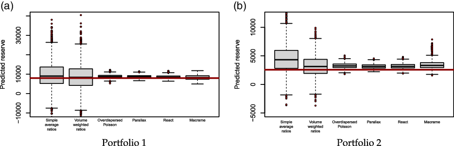
The same two portfolios from Figure 1 are once again compared, now in terms of the overall reserve distributions derived from the bootstrap samples and the given reserving methods, see Figure 6. For the first portfolio in Figure 6(a), which is ODP compliant (i.e., all the incremental claim amounts are strictly positive), our non-parametric approaches to reserving techniques compete well with the standard parametric methods. Especially, PARALLAX and REACT beat the remaining reserving techniques in terms of variability. The most accurate result with respect to the point prediction is MACRAME (although more volatile than PARALLAX or REACT, but still better than the standard methods based on averaging development ratios). For the second portfolio in Figure 6(b) – which is still ODP compliant according to the observed upper part of the triangle, but it is not ODP compliant according to its further development (lower triangle) – our reserving techniques together with the ODP model come as more suitable. The negative incremental claim amounts present solely in the unobserved part of the square cause that all of the reserving methods provide biased results. However, PARALLAX still shows the smallest variability, in terms of interquartile range.
Bootstrap reserve distributions for three standard methods from Section 2 and three functional profile based approaches from Section 3. The red thick horizontal line corresponds to the true reserve. The upper whiskers corresponding to the 95%-quantiles are above the true reserve for all the methods.

6. Empirical comparisons via retrospective testing
In this section, we investigate the overall empirical performance of the proposed methods, comparing them also to the traditional reserving techniques described in Section 2, on the 518 run-off triangles from the National Association of Insurance Commissioners database (Meyers and Shi, Reference Meyers and Shi2011b). We stress the conceptual difference here: contrary to synthetic data created by simulations that follow postulated assumptions, this comparison is done on an extensive and representative collection of real data from the insurance industry, which includes, among other things, various non-standard triangles – triangles that could be considered atypical from the theoretical point of view, but nevertheless occur in the actuarial practice.
6.1. The description of the database
The run-off triangles of paid losses correspond to claims of accident years 1988–1997 with
 $n = 10$
years development period, relating to six different lines of business (private passenger auto liability/medical, commercial auto/truck liability/medical, workers’ compensation, medical malpractice, other liability, and product liability) from the US property-casualty insurers. We a priori eliminated triangles with only zero observed claim amounts in the last four accident periods and also those triangles having 8 or more development profiles identically equal to zero (which can occur, e.g., when the company does not show recent activity or it does not run the particular line of business (LoB) anymore).
The remaining run-off triangles were split – from the actuarial viewpoint, and also in view of the applicability of standard methods – into three groups: (i) 130 run-off triangles that were ODP compliant (with only non-negative increments, but profiles being entirely zero not allowed); (ii) 299 not ODP compliant triangles (negative increments exist, but still no entirely zero profiles); (iii) 89 remaining triangles that could be considered “rather atypical,” but are still not uncommon in the actuarial practice (for instance, those with development profiles consisting entirely of zeros; we allowed triangles with up to 7 such profiles out of 10 development periods).
6.2. Claims reserves evaluation
For each run-off triangle, the overall claims reserve was estimated via the techniques described in Sections 2 and 3. The stochastic prediction was obtained from the corresponding bootstrap add-on (Section 5), and the quality of the prediction was subsequently evaluated with respect to the true reserve (which is in this case known, as all the data feature the lower parts, the triangles being fully completed). The overall quality of the reserve prediction was evaluated in terms of four quantitative criteria motivated by the standard out-of-sample bootstrap performance measures (e.g., Efron and Tibshirani, Reference Efron and Tibshirani1993, Chapter 19):
Reserve% gives an absolute relative difference of the predicted reserve and the true reserve defined for each triangle as
 \begin{equation*}100 \times \left|\frac{\textrm{predicted reserve}}{\textrm{true reserve}} - 1\right|,\end{equation*}
and averaged over all triangles in the given scenario (smaller values are better);
BootCoV% expresses a coefficient of variation for the bootstrapped reserve distribution relative to the bootstrap mean
 \begin{equation*}100 \times \frac{\textrm{Std.Dev}(\textrm{bootstrapped reserves})}{\textrm{Avg}(\textrm{bootstrapped reserves})},\end{equation*}
averaged, again, over all triangles in the given scenario (smaller values are better);
BootVaR
 $_{\boldsymbol{.995}}$
denotes the
 $99.5\%$
quantile of the bootstrap distribution relative to the bootstrapped mean
 \begin{equation*}\frac{\textrm{Quantile$_{0.995}$}(\textrm{bootstrapped reserves})}{\textrm{Avg}(\textrm{bootstrapped reserves})},\end{equation*}
and averaged over all triangles in the given scenario (smaller values are better);
BootQnt
 $_{\boldsymbol{.950}}$
provides a percentage proportion of the triangles in the given scenario for which the true reserve is dominated by the 95% quantile of the bootstrapped distribution (values closest to 95% are preferred).
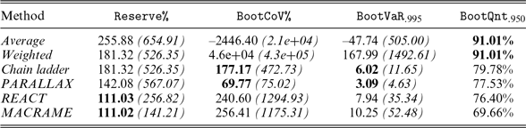
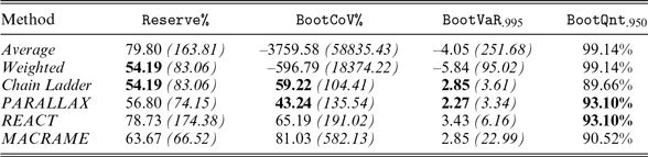
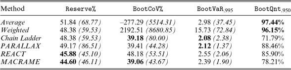
The results for the groups (i), (ii), and (iii) are reported in Tables 2, 3, and 4, respectively. In addition, we also considered the run-off triangles from two particular lines of business (commercial auto/truck liability/medical and workers’ compensation) and analogous results are given in Tables 5 and 6. The actual choice of B is a problem of itself, requiring theoretical/empirical study beyond the scope of this paper. We observed that
 $B=10{,}000$
yielded results sufficiently stable for our objectives.
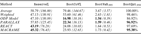
Overall empirical performance of six claims reserving techniques when applied to the group (i), 130 ODP compliant run-off triangles from Meyers and Shi (Reference Meyers and Shi2011b). The corresponding standard deviations are given in parentheses; two best results are indicated by bold typeface.

Empirical performance of six claims reserving techniques applied to the group (ii), 299 “rather typical” but ODP non-compliant run-off triangles from Meyers and Shi (Reference Meyers and Shi2011b). The corresponding standard deviations are given in parentheses; two best results are indicated by bold typeface.

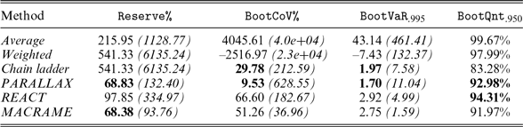
Empirical performance of six claims reserving techniques applied to the group (iii), 89 “atypical” run-off triangles from Meyers and Shi (Reference Meyers and Shi2011b). The corresponding standard deviations are given in parentheses; two best results are indicated by bold typeface.

Empirical performance of six claims reserving techniques when applied to 116 run-off triangles for the “commercial auto/truck liability/medical” line of business from Meyers and Shi (Reference Meyers and Shi2011b). The corresponding standard deviations are given in parentheses; two best results are indicated by bold typeface.

Empirical performance of six claims reserving techniques when applied to 132 run-off triangles for the “workers’ compensation” line of business from Meyers and Shi (Reference Meyers and Shi2011b). The corresponding standard deviations are given in parentheses; two best results are indicated by bold typeface.

Regarding the reserve prediction, all six methods in Table 2 perform rather similarly. Indeed, the decent performance of the traditional parametric methods is in particular to be expected for the ODP compliant loss development run-off triangles, as those satisfy the parametric model assumptions. However, new methods are in this situation still competitive and two out of three (REACT and MACRAME) even outperform all parametric ones. As far as the prediction of the overall reserve distribution by the bootstrap extension is considered, only the ODP model from parametric reserving techniques seems to provide solid results closely followed by all three functional approaches. However, only 87% of the true reserves are dominated by the 95% quantile of the ODP model-based bootstrap distribution while the best performance is guaranteed for the permutation based bootstrap, most precisely by MACRAME (
 $95.38\%$
).
The situation becomes different in Table 3, when the run-off triangles are not ODP compliant (and thus the ODP model is inapplicable). Traditionally, the chain ladder model relying on (14) is utilized as an alternative for point predictions in this case. We adopted the same strategy in our numerical comparisons. The nave approaches based on development ratios fail here: both in the reserve prediction and the reserve distribution bootstrapping. The superiority of the proposed PARALLAX, REACT, and MACRAME algorithms is evident especially in terms of the reserve prediction (Reserve%). For the bootstrap distribution, the chain ladder method is the only competitive parametric technique, but it again fails in terms of the true reserve coverage (BootQnt
 $_{.950}$
).
In Table 4, the performance of the standard parametric techniques does not appear reasonable except for the chain ladder method which is, however, inapplicable in its straightforward form for this type of run-off triangles. The reason is that zero values may appear in the denominator in (14). In practice, this is mitigated by various modifications, typically requiring additional expert insights or the estimates of the problematic development factors are set to one by default. This was also the case in our empirical comparison. Our methods run without any modifications and all three of them outperform parametric techniques in terms of the reserve prediction (Reserve%) while performing very similarly as the modified chain ladder method in terms of the bootstrap distribution (PARALLAX still dominates).
Finally, we also compared the performance of all six reserving techniques (using the same four quantitative criteria) when applied to the run-off triangles from the same underlying LoB. Two different LoBs are considered: commercial auto/truck liability/medical as a portfolio which is expected to have rather less atypical triangles and the workers’ compensation portfolio with a long-tailed liability and rather more atypical triangles. The results are summarized in Table 5 and 6.
The chain ladder method and all three proposed functional techniques perform very similarly for both portfolios: the “commercial auto/truck liability/medical” LoB and the “workers’ compensation” liability. The parametric chain ladder is slightly better in reserve prediction (Reserve%) in the first LoB; our methods perform better in terms of the bootstrap distribution in both LoBs. However, the chain ladder method gets the worst coverage scores (BootQnt
 $_{0.950}$
) in both portfolios.
From the overall point of view, ignoring the triangle types as well as the LoB, the 95% upper-sided prediction interval from the chain ladder covers only
 $83.59\%$
of the true reserves for all 518 triangles and, therefore, the chain ladder undershoots the theoretical value of 95%. On the other hand, this overall empirical prediction coverage for the true reserves becomes better for all three proposed functional profile methods:
 $91.67\%$
for PARALLAX,
 $92.08\%$
for REACT, and
 $89.00\%$
for MACRAME.
7. Conclusions
Claims reserving is a key task in insurance business, as a rule formally stipulated by various regulatory codes. Routinely used approaches for risk reserving assessment are based on the chain ladder or generalized linear models, with various bootstrap extensions. While bootstrapping may be performed for wide range of different situations and consequently is not that much restricted by theoretical assumptions, chain ladder and generalized linear models heavily rely on various assumptions, rather crucial for the overall model validity and applicability. Many portfolios must be, therefore, evaluated using alternative approaches.
In this paper, we propose loss reserving techniques based on non-parametric and distribution free approaches. The proposed methods offer the following advantages: (i) they are simple, straightforward, and easily applicable; (ii) they require neither distributional nor parametric assumptions and apply to all kinds of run-off triangles, including those with negative incremental cells or zero cumulative claim amounts over some development periods; (iii) various stochastic model assumptions can be postulated in order to derive desirable statistical properties serving as the methods’ justifications; (iv) it is straightforward to obtain also the overall reserve distributions via bootstrapping techniques; (v) and the proposed methods are also robust against outliers. When compared to retrospective, historical data (on the complete squared, i.e., with predicted reserves already observed, run-off triangles), the new methods demonstrate apparent superiority over traditional claims reserving techniques – a clear indication of their potential in the actuarial practice.
Of course, summarizing and comparing methods proposed here, we need to be aware of their distribution free, non-parametric design. While this means independence of restrictive assumptions and wider range of applications, it can also cause somewhat higher volatility in the prediction of the claims reserves. However, if the distributional/parametric assumptions are violated, the classical reserving approaches may yield unreliable reserve predictions – or even collapse, as demonstrated on the triangles still common in actuarial practice. Hence, we advocate some caution when using traditional reserving techniques; at least, they should be accompanied by the proper diagnostics of the underlying assumptions.
The practical guidelines for applying the proposed methods may still need some further investigation, and above all, practical experience. So far, we observed that while the PARALLAX could be recommended for cumulative run-off triangles possessing unpredictable trend fluctuations across the accident years, the REACT works well when the behavior of an insurance company in a given year is likely to be similar (up to possible trend) to that in the previous/forthcoming year. Finally, the MACRAME is applicable overall, even if the portfolio size is increasing. It is more robust, but it also allows the actuary to intervene into the model, for instance, by specifying the states of the Markov chain using some expert insight rather than the fully data-driven approach.
Acknowledgement
The authors thank the associate editor and three reviewers for their insights and valuable remarks that greatly improved this work. Matúš Maciak and Michal Pešta acknowledge financial support by the Czech Science Foundation project GACR No. 18-01781Y. The research of Ivan Mizera was supported by the NSERC of Canada. The authors would like to express their thanks to the Banff International Research Station (BIRS) in Banff, Alberta, Canada, for hosting them in the “research in teams’‘ program in August 2014 (Statistical Predictions for Chain Ladder Data (14rit206): http://www.birs.ca/events/2014/research-in-teams/14rit206). The fundamentals of the research published in the paper where mostly laid down in the beautiful surroundings of the Banff National Park.
Supplementary material
To view supplementary material for this article, please visit https://doi.org/10.1017/asb.2022.4.