Housing Speculation and Investment in Children’s Education: Evidence from House Purchase Restrictions in China

Geng Niu; Xuefeng Xiang; Liuming Yang; Yang Zhou

doi:10.1017/S0022109026102713

Housing Speculation and Investment in Children’s Education: Evidence from House Purchase Restrictions in China

Published online by Cambridge University Press: 24 February 2026

Liuming Yang and

Geng Niu: Affiliation:
Southwestern University of Finance and Economics Research Institute of Economics and Management g.niu@swufe.edu.cn
Xuefeng Xiang: Affiliation:
Southwestern University of Finance and Economics Research Institute of Economics and Management XuefengXiang1995@163.com
Liuming Yang: Affiliation:
The Chinese University of Hong Kong Business School liumingyang@cuhk.edu.hk
Yang Zhou*: Affiliation:
Wuhan University Economics and Management School
*: y.zhou@whu.edu.cn (corresponding author)

Article contents

Abstract
Introduction
Institutional Background and Conceptual Framework
Data, Variables, and Empirical Strategy
Empirical Results
Further Analysis
Welfare Implications
Conclusion
Funding Statement
Footnotes
References

Rights & Permissions

Abstract

Housing and human capital represent two major forms of household wealth. This article investigates the potential for housing speculation to crowd out household investment in children’s education, an endeavor that only pays off in the long run. To address endogeneity concerns, we exploit the unintended spillover effect of staggered house purchase restrictions (HPR) in China. Using a difference-in-differences approach, we find that HPR reduce educational investment of households in nearby unregulated cities. We also provide evidence consistent with a housing speculation channel. These findings shed new light on the socioeconomic consequences of housing market booms.

Information

Type: Research Article
Information: Journal of Financial and Quantitative Analysis , Volume 61 , Issue 6 , September 2026, pp. 3113 - 3140
DOI: https://doi.org/10.1017/S0022109026102713 [Opens in a new window]
Copyright: © The Author(s), 2026. Published by Cambridge University Press on behalf of the Michael G. Foster School of Business, University of Washington

I. Introduction

Housing is the dominant asset on household balance sheets, and fluctuations in its value can significantly shape household behavior with broad economic consequences (Mian, Sufi, and Trebbi (Reference Mian, Sufi and Trebbi2015)). Prior research shows that rising house prices affect not only current households but also children’s outcomes, as wealth effects from perceived wealth or borrowing capacity influence schooling decisions (Lovenheim (Reference Lovenheim2011), Lovenheim and Reynolds (Reference Lovenheim and Reynolds2013)). More recent work highlights a different mechanism: house price booms raise expectations of future growth, fueling speculation (Gao, Sockin, and Xiong (Reference Gao, Sockin and Xiong2020), Mian and Sufi (Reference Mian and Sufi2022)). Such speculation may crowd out nonhousing investments, including children’s education. This aspect remains largely unexamined, and our study seeks to fill this gap by exploring a speculation channel through which housing booms may crowd out investment in children’s education.

Since the development of human capital theory (Becker (Reference Becker1967)), education spending has been viewed as an investment in future labor market earnings. Under budget constraints, however, housing and education may act as substitutes. Human capital investment is long term, requiring time before returns materialize (Hanushek, Kinne, Lergetporer, and Woessmann (Reference Hanushek, Kinne, Lergetporer and Woessmann2021)), whereas housing speculation can yield quicker gains. During housing booms, rising optimism and strong beliefs in further price growth (Glaeser and Nathanson (Reference Glaeser and Nathanson2017), Gao et al. (Reference Gao, Sockin and Xiong2020)) raise the perceived opportunity cost of education. At the same time, higher housing wealth may enhance the capacity to invest in children’s education. This tension makes the relationship between housing market dynamics and educational investment an important empirical question.

Identifying the causal effect of housing market dynamics on educational investment is challenging because unobserved local characteristics may drive both. China offers a suitable setting: since 2000, it has experienced a major housing boom that is difficult to reconcile with fundamentals (Glaeser and Nathanson (Reference Glaeser and Nathanson2017), Han, Han, and Zhu (Reference Han, Han and Zhu2018)). To address worsening affordability, governments introduced house purchase restrictions (HPR), which cooled prices in regulated cities but spurred capital flows and sharp price increases in nearby unregulated ones (Deng, Liao, Yu, and Zhang (Reference Deng, Liao, Yu and Zhang2022)). Importantly, the timing and jurisdiction of HPR varied, enabling a difference-in-differences (DID) design. Specifically, we compare educational investment of households in unregulated cities that are geographically close to regulated cities (treatment group) to that of households in unregulated cities that are farther away from regulated cities (control group). While the decision to impose HPR is endogenous to local conditions, the induced spillovers to surrounding unregulated cities are arguably exogenous, as restrictions were based on regulated cities’ fundamentals rather than those of neighboring areas. Thus, the HPR-induced booms in nearby cities provide plausibly exogenous variation that supports a causal interpretation.

Using data from the China Household Finance Survey (CHFS) for the period 2011–2021, we find that households in nearby nonrestricted cities (within 250 km of restricted cities) significantly reduce educational investment by 25.15% following the implementation of the HPR compared to those in farther away cities. Our results remain robust to a range of checks, including a parallel trends test, alternative definitions of treated cities, the inclusion of additional controls, and adjustments for heterogeneous treatment effects. In particular, an intuitive competing transmission channel is that our findings merely reflect rising living costs in nearby unregulated cities following the HPR shock. We mitigate this concern by showing that our estimates remain robust after controlling for local inflation, indicating that the observed effect is not driven by changes in the cost of living.

We continue with various tests to verify the housing speculation channel. First, we show that following the HPR policy shock, both house prices and household attention to the housing market increase significantly in nearby unregulated cities. Moreover, expectations of future house price growth and the likelihood of planning to invest in housing also rise in these areas. These results indicate that the HPR policy heightens households’ speculative motives in treated cities. Next, we document that households in treated cities reduce discretionary consumption and stock market investment. This pattern suggests that households may be reallocating financial resources for housing investment. Complementing this, survey responses reveal that treated households are more likely to report needing funds for house purchase and less likely to report needing funds for children’s education. Finally, we show that these households lower their aspirations for their children’s education. Overall, these results are consistent with households reallocating resources away from education and toward housing investment.

We also perform a series of heterogeneity analyses to further illuminate our findings. First, we show that the negative effect of the HPR policy is more pronounced for households with lower levels of wealth and education. This pattern is consistent with the notion that financially less constrained families are less likely to reallocate resources from education to housing, while parents with higher education are more likely to recognize both the pecuniary and nonpecuniary returns to education (Oreopoulos and Salvanes (Reference Oreopoulos and Salvanes2011)). Second, we find that the negative spillover effect of HPR holds across households with children of all ages, and the differences across age groups are not statistically significant. This result casts doubt on the interpretation that housing serves primarily as a savings vehicle for children’s college education, since the HPR effect persists even among households with children already in college. Moreover, it suggests that our findings are not simply driven by changes in labor market opportunities, as the crowding-out effect is also significant for households with nonworking-age children. Third, we find that the spillover effect of HPR is stronger among households that acquired additional property following the policy shock.

Finally, we conduct subsample analyses that distinguish between single- and multiple-home owners. We find that the crowding-out effect of HPR on education and discretionary spending is driven primarily by single-home owners rather than multiple-home owners. This finding is consistent with the notion that multiple-home owners experience a stronger wealth effect from rising housing prices.

Our article contributes to three strands of literature. First, it relates to studies on the economic consequences of housing market dynamics, including effects on labor supply (Johnson (Reference Johnson2014), Zhao and Burge (Reference Zhao and Burge2017), Disney and Gathergood (Reference Disney and Gathergood2018), and Glancy (Reference Glancy2021)), consumption (Gan (Reference Gan2010), Musso, Neri, and Stracca (Reference Musso, Neri and Stracca2011), Mian, Rao, and Sufi (Reference Mian, Rao and Sufi2013), Agarwal and Qian (Reference Agarwal and Qian2017), and Kartashova and Tomlin (Reference Kartashova and Tomlin2017)), and entrepreneurship (Adelino, Schoar, and Severino (Reference Adelino, Schoar and Severino2015), Corradin and Popov (Reference Corradin and Popov2015), Schmalz, Sraer, and Thesmar (Reference Schmalz, Sraer and Thesmar2017), and Tian and Wang (Reference Tian and Wang2025)). Housing values also affect education: while house price gains have been shown to increase college enrollment through wealth and borrowing capacity (Lovenheim (Reference Lovenheim2011), Lovenheim and Reynolds (Reference Lovenheim and Reynolds2013), and Johnson (Reference Johnson2020)), their potential negative effects are less explored. Charles, Hurst, and Notowidigdo (Reference Charles, Hurst and Notowidigdo2018) find that booms can reduce enrollment by raising the opportunity cost of college. We add new evidence by identifying a crowding-out effect of housing booms on educational investment through a speculation channel.

Moreover, our study also contributes to the literature on housing speculation. Prior work shows that speculation fuels booms and busts (Gao et al. (Reference Gao, Sockin and Xiong2020)), is amplified by credit supply expansions (Mian and Sufi (Reference Mian and Sufi2022)), and can be triggered by policies such as LTV limits on second-home purchases in China (Chen, Wang, Xu, and Zha (Reference Chen, Wang, Xu and Zha2022)). We add to this line of research by documenting a micro-level consequence: a crowding-out effect whereby household capital shifts from educational investment to housing investment. As educational investment is crucial for long-term and sustainable economic growth (Aghion and Howitt (Reference Aghion and Howitt2008)), our findings offer a new perspective to understand the real and unexpected consequences of housing speculation.

Lastly, our article is linked to research on the effect of housing regulation. While the existing literature has primarily focused on the direct effect of government interventions in housing markets (Fu, Qian, and Yeung (Reference Fu, Qian and Yeung2016), Han, Lutz, Sand, and Stacey (Reference Han, Lutz, Sand and Stacey2021)), our article examines the spillover effect of the HPR policy on households located in nearby unregulated cities by analyzing its unintended consequence on investment in children’s education. The findings suggest that policymakers should pay attention to the potential spillover effect of housing regulations.

II. Institutional Background and Conceptual Framework

China has witnessed a remarkable housing boom since 2003 (Liu and Xiong (Reference Liu, Xiong, Amstad, Sun and Xiong2020)). For example, between 2003 and 2011, the average annual growth rate of house prices was around 17% across major cities in China and exceeded 20% in megacities such as Beijing and Guangzhou (Fang, Gu, Xiong, and Zhou (Reference Fang, Gu, Xiong and Zhou2016)).Footnote ¹ This dramatic real estate boom prompted substantial concerns within the Chinese government, as the high growth rate of house prices was argued to generate negative externalities for the real economy (Glaeser, Huang, Ma, and Shleifer (Reference Glaeser, Huang, Ma and Shleifer2017)). As a result, the Chinese central government introduced measures intended to rein in the housing market by imposing the HPR policy.

The HPR policy included a series of restrictions such as limiting the number of houses a family could purchase, increasing the down payment ratio, and setting a minimum residency requirement before buying a property in regulated cities. The implementation of the HPR policy had considerable variations by jurisdiction and timing (Deng et al. (Reference Deng, Liao, Yu and Zhang2022), Tian and Wang (Reference Tian and Wang2025)). The HPR policy primarily focused on cooling the property market in tier-one cities, as well as preventing speculative investment in tier-two and tier-three cities.

While the policy was considerably effective in containing rising house prices in the regulated cities, it created a positive spillover effect on house prices in nearby unregulated cities. As shown by Deng et al. (Reference Deng, Liao, Yu and Zhang2022), capital spilled from regulated cities to nearby cities due to the increased transaction costs in regulated cities, leading to a surge and boom in house prices in unregulated housing markets. Such a positive spillover effect is stronger for nearby non-HPR cities than for those located farther away.

A sharp rise in local house prices can simultaneously boost expectations of future appreciation and depress rental yields. We argue that in nearby unregulated cities, the former effect dominates, making housing speculation more attractive. Households tend to extrapolate recent price trends (Glaeser and Nathanson (Reference Glaeser and Nathanson2017), Kuchler, Piazzesi, and Stroebel (Reference Kuchler, Piazzesi, Stroebel, Bachmann, Topa and van der Klaauw2023)), and evidence shows that such expectations shape real decisions (Armona, Fuster, and Zafar (Reference Armona, Fuster and Zafar2019)). Given the surge in treated cities, households had strong incentives to speculate on further gains. This emphasis on capital gains over rental returns is consistent with China’s high price-to-rent ratios and low user costs (Glaeser et al. (Reference Glaeser, Huang, Ma and Shleifer2017)).

The (perceived) opportunity of housing speculation could be particularly appealing in China as Chinese households have limited investment opportunities: the real interest rate on bank deposits is low, the domestic stock market and bond market are underdeveloped, and the tight capital controls restrict investing abroad.

As household resources are limited, increasing the investment in one asset tends to reduce resources for other purposes. The problem of limited budgets might particularly be a concern for households in our study. For example, unlike in developed countries, it is challenging for homeowners in China to extract equity from homes that have appreciated in value owing to underdeveloped mortgage markets and strict policy restrictions (Painter, Yang, and Zhong (Reference Painter, Yang and Zhong2022)). Moreover, during our sample period, China’s cautious credit policies resulted in notably higher mortgage rates and down payment requirements compared to the United States (Glaeser et al. (Reference Glaeser, Huang, Ma and Shleifer2017)).

An important but intangible asset for a household is the human capital of children, which affects children’s labor market earnings in the future (Becker (Reference Becker1967)). Increasing children’s ultimate educational outcomes often requires a constant and nontrivial input of monetary and nonmonetary resources. However, educational investment normally takes a long time to take effect and even longer before returns materialize (Hanushek et al. (Reference Hanushek, Kinne, Lergetporer and Woessmann2021)). Hence, we conjecture that increased incentives to speculate in housing would induce households to curtail their educational investment in children.

It is important to recognize that parental investment in children’s education may be driven by both pecuniary and nonpecuniary motives, including altruism, bequest considerations, and aspirations for intergenerational mobility. In this context, the crowding-out channel we propose can be viewed in two ways: as a portfolio reallocation between housing assets and human capital and as a shift between (educational) consumption and (housing) investment. This nuance does not alter the core trade-off, that is, housing speculation crowds out education, so we do not distinguish between these interpretations in our study.

III. Data, Variables, and Empirical Strategy

A. Data and Variables

Our main data set is the CHFS, which is a countrywide longitudinal survey conducted by the Research Center for the CHFS at Southwestern University of Finance and Economics (SWUFE). The CHFS has been widely used in studies on household finance in China, including those investigating household savings (Chen, Chen, and He (Reference Chen, Chen and He2019)), investment (Liang and Guo (Reference Liang and Guo2015)), and entrepreneurship (Fan, Li, Li, and Zhang (Reference Fan, Li, Li and Zhang2022)), to name a few. The survey collects detailed demographic information from respondents every 2 years starting from 2011, including city of residence, homeownership status, age, wealth, income, family size, and children’s information. We leverage data from six waves, 2011, 2013, 2015, 2017, 2019, and 2021, to form an unbalanced household-level panel data set.

Our main dependent variable is the natural logarithm of investment in children’s education. Following the literature (Jia, Zhou, and Yang (Reference Jia, Zhou and Yang2021), Wang et al. (Reference Wang, Cheng and Smyth2022)), we measure educational investment as the sum of tuition fees, tutoring expenses, costs of extracurricular activities, books and supplies, and other education-related materials and equipment.Footnote ²

To capture the spillover effect of the HPR policy, we manually collected the list of implementing cities and their enactment and suspension dates from official government websites. Following Deng et al. (Reference Deng, Liao, Yu and Zhang2022), we construct our core explanatory variable, HPR_250 km_jt, a dummy variable that equals 1 if an unregulated city j is within 250 km of any city under the HPR in year t, and 0 otherwise.

Two points are worth noting. First, following Deng et al. (Reference Deng, Liao, Yu and Zhang2022), this article uses 250 km as the benchmark threshold for identifying spillover effects of the HPR policy. The underlying rationale is that with the development of high-speed rail, a round trip between cities within 250 km can be completed within 2 h, greatly facilitating cross-city real estate investment and capital flows. Within this range, investors can also easily inspect and manage properties. To ensure our results are not sensitive to this choice, we test alternative thresholds of 100 and 150 km in robustness checks. Second, HPR_250 km_jt can be treated as a dummy variable that indicates whether households in nonregulated cities experienced a sharp increase in house prices. Since our goal is to study the impact of house price increases on household educational investment, this variable serves to capture a positive shock to local house prices.

To account for individual heterogeneity that might affect the relationship between HPR spillover and educational investment, we incorporate a comprehensive set of household- and city-level control variables. As we control for household fixed effects in our empirical models, we focus on time-varying household characteristics, such as the age of the household head, family size, family wealth and income, and the number of children in different age groups. At the city level, we control for GDP per capita, population density, fiscal expenditure, fiscal revenue, employment, average wage, financial development, industrial structure, real estate investment, and the number of secondary and primary school teachers. These city-level variables are extracted from the China Stock Market and Accounting Research Database (CSMAR).

B. Sample Construction

Based on our research question, the raw CHFS data are processed as follows: First, we keep only families with children still in school. Second, we retain homeowner households for two reasons. For one, there is a fundamental difference in investment decisions between tenants and homeowners. As homeowners already possess property, they tend to have a stronger speculation incentive than tenants do (Gao et al. (Reference Gao, Sockin and Xiong2020)). The other reason is that homeowners constitute the vast majority of the sample, accounting for around 90% of the total observations.Footnote ³ Third, we restrict the sample to households located outside HPR cities. Fourth, we exclude households that changed residences during the sample period.Footnote ⁴ Fifth, to satisfy the standard staggered DID assumption, we exclude households that switch in and out of treatment, that is, nonabsorbing treatments. Finally, after matching the CHFS data to macro-level data and removing observations with any missing values, we obtain an unbalanced panel with 17,863 observations. The number of households in each wave is as follows: 955 (2011), 2,132 (2013), 4,018 (2015), 4,821 (2017), 3,494 (2019), and 2,443 (2021).

Table 1 provides summary statistics for the variables outlined previously. The average annual educational investment is 7,066 RMB, which is consistent with values reported in the literature (e.g., Wang, Cheng, and Smyth (Reference Wang, Cheng and Smyth2022), Chen, Yuan, and Zhang (Reference Chen, Yuan and Zhang2023)). The median number of children per household is 1, which is consistent with the long-established one-child policy in China. The median household size is 4. Despite the one-child policy, household size in China could be larger than 3 due to the prevalence of intergenerational coresidence, which is common in China owing to strong family ties and cultural traditions. Multigenerational living is widely viewed as an ideal structure in China and plays an essential role in providing support and care within the family (Xu (Reference Xu2019)). It is particularly common for grandparents to live with their adult children to help care for their grandchildren. Additional details on the sample and empirical analysis are provided in the Supplementary Material.

TABLE 1Summary Statistics

A summary statistics table for 24 variables including educational investment, household demographics, and regional economic indicators for 17,863 observations. See long description.

TABLE 1 Long description

The table contains summary statistics for 17,863 observations across various metrics.

Key variables include:

* Educational investment: Mean 7,066.323, Median 3,300, Min 30, Max 400,000, Std. Dev. 11,218.623.

* Log Educational investment: Mean 7.673, Median 8.102, Min 3.401, Max 12.899, Std. Dev. 1.923.

* H P R _ 250 km: Mean 0.489, Median 0, Min 0, Max 1, Std. Dev. 0.384.

* Age: Mean 47.803, Median 46, Min 18, Max 95, Std. Dev. 11.144.

* Household size: Mean 4.632, Median 4, Min 2, Max 16, Std. Dev. 1.474.

* Log Household income: Mean 10.046, Median 10.609, Min 0, Max 15.416, Std. Dev. 2.283.

* Log Household wealth: Mean 12.538, Median 12.672, Min 3.912, Max 16.811, Std. Dev. 1.308.

* Number of children: Mean 1.511, Median 1, Min 1, Max 8, Std. Dev. 0.721.

* Educational counts (Preschool to College): Means range from 0.144 (College) to 0.552 (Primary school).

* Regional Economic Indicators (Log values): G D P per capita (Mean 10.593), Population density (Mean 5.621), Fiscal expenditure (Mean 15.093), Fiscal revenue (Mean 13.970), Employment (Mean 12.898), Average wage (Mean 10.909), and Loans (Mean 16.729).

* Tertiary Industry: Mean 0.404, Median 0.403, Min 0.188, Max 0.817, Std. Dev. 0.076.

* Log Real estate investment: Mean 14.153, Median 14.038, Min 10.168, Max 17.715, Std. Dev. 1.214.

* Teacher counts (Log values): Secondary teacher (Mean 9.762) and Primary teacher (Mean 9.783).

C. Empirical Design

In China, while the HPR policy is formulated by the central government, its implementation is delegated to local governments. Consequently, the introduction of HPR in regulated cities is endogenous, as it is influenced by numerous local economic and institutional factors. This article, however, investigates the spillover effect of HPR on nearby unregulated cities. We argue that since the decision to implement home purchase restrictions is mainly determined by the regulated city’s own economic conditions instead of those of surrounding cities, the HPR policy can be considered relatively exogenous for surrounding unregulated cities. To some extent, this alleviates potential endogeneity concerns. Following Deng et al. (Reference Deng, Liao, Yu and Zhang2022), we use the sudden surge and boom in house prices in nearby unregulated cities that are induced by the unintended geographical spillover generated by the HPR policies as our main identification strategy. We classify households in nearby unregulated cities as the treatment group and those in remote unregulated cities as the control group and perform a standard staggered DID analysis. The regression model is specified as

(1) $$ {Y}_{ijt}={\beta}_0+{\beta}_1HPR\_250\ {km}_{jt}+{\beta}_2{X}_{ijt}+{\beta}_3{Z}_{jt}+{\gamma}_i+{\tau}_t+{\varepsilon}_{ijt,} $$

where $ {Y}_{ijt} $ represents the natural logarithm of educational investment for family i in city j at time t. $ HPR\_250\;{km}_{jt} $ is our key independent variable, which is a dummy variable that equals 1 if city j is within 250 km of a HPR city at time t, and 0 otherwise. $ {X}_{ijt} $ and $ {Z}_{jt} $ are vectors of household- and city-level time-varying characteristics outlined previously. We further control for household fixed effects ( $ {\gamma}_i $ ) and year fixed effects ( $ {\tau}_t $ ) to account for shocks that are household- and time-specific. The standard errors are clustered at the city level to account for the correlations in educational investment of households living in the same city.

Note that because the survey is conducted biennially, the reference wave is set to the implementation year itself if it is an odd number. If the implementation year is an even number, the reference wave is assigned to the following (odd) year. For example, a policy enacted in 2014 (even) would use 2015 as the reference wave, while a policy enacted in 2013 (odd) would use 2013 as the reference wave.

IV. Empirical Results

A. Benchmark Results

Table 2 reports the baseline results examining the spillover effect of the HPR policy on household educational investment in unregulated cities. In column 1 without controls, the regression coefficient of HPR_250 km is negative and significant at the 5% level. This suggests that the spillover effect of the HPR policy has led to a significant decrease in educational investment of families in unregulated cities that are geographically close to regulated cities compared with that of families located in distant unregulated cities. After adding household-level controls in column 2, the regression coefficient of HPR_250 km remains significantly negative. When we include both household- and city-level characteristics in column 3, the coefficient of interest continues to be negative and highly significant. Taken together, these findings reveal a negative spillover effect of the HPR policy on educational investment by households in nearby unregulated cities.

TABLE 2Benchmark Results

A regression table showing benchmark results for Log Educational Investment across three models. See long description.

TABLE 2 Long description

The table presents regression coefficients with standard errors in parentheses for three models labeled 1, 2, and 3. The dependent variable is Log Educational Investment.

* H P R 250 km: Model 1 is minus 0.2422 (0.0931); Model 2 is minus 0.2411 (0.0922); Model 3 is minus 0.2515 (0.0958). All are statistically significant.

* Age: Model 2 and 3 are both minus 0.0025 (0.0025).

* Household size: Model 2 is 0.0203 (0.0325); Model 3 is 0.0217 (0.0326).

* Log Household income: Model 2 is 0.0199 (0.0087); Model 3 is 0.0208 (0.0088).

* Log Household wealth: Model 2 is 0.0585 (0.0246); Model 3 is 0.0622 (0.0238).

* No. of preschool: Model 2 is 0.4064 (0.0710); Model 3 is 0.4038 (0.0714).

* No. of primary school: Model 2 is 0.2465 (0.0566); Model 3 is 0.2508 (0.0558).

* No. of junior high school: Model 2 is 0.3608 (0.0682); Model 3 is 0.3671 (0.0669).

* No. of senior high school: Model 2 is 0.7965 (0.0784); Model 3 is 0.8012 (0.0790).

* No. of college: Model 2 is 0.8061 (0.0898); Model 3 is 0.8154 (0.0902).

* Model 3 includes additional controls: Log G D P per capita 0.4647 (0.1655); Log Population density 0.1574 (0.0857); Log Fiscal revenue minus 0.4131 (0.1692); and Log No. of secondary teacher 0.4266 (0.2521).

* Fixed Effects: All models include Year F E and Household F E.

* Statistics: Number of observations is 17,863 for all models. R-squared values are 0.5301 for Model 1, 0.5458 for Model 2, and 0.5475 for Model 3.

In terms of economic magnitude, the estimate of HPR_250 km in column 3 is −0.2515, which implies that educational investment of households in nearby unregulated cities decreases by 25.15% compared to those in faraway cities after the HPR policy shock. Given the sample mean of 7,066 RMB, this translates to a 1,777 RMB decline in educational investment per year. Using the estimated impact of the HPR shock on housing prices in treated cities (0.1102), we calculate the elasticity of educational investment with respect to housing price appreciation. The implied elasticity is 2.28 (0.2515/0.1102), indicating that a 1% increase in housing prices induced by the HPR policy in nearby unregulated cities is associated with approximately a 2.28% decline in educational investment. This result suggests that the negative spillover effect of HPR on educational investment is economically significant.

The nontrivial economic magnitude can be understood within China’s institutional context. For example, underdeveloped mortgage markets and policy restrictions prevent Chinese households from extracting home equity (Painter et al. (Reference Painter, Yang and Zhong2022)). In addition, China adopted prudent credit policies for the housing market during our sample period. Specifically, mortgage interest rates in China tended to exceed those in the United States significantly, and down payment thresholds were also notably high, especially for the second house (Glaeser et al. (Reference Glaeser, Huang, Ma and Shleifer2017)). Therefore, households may have had to cut a substantial portion of educational expenses for housing investment.

B. Robustness Checks

1. Parallel Trends Test

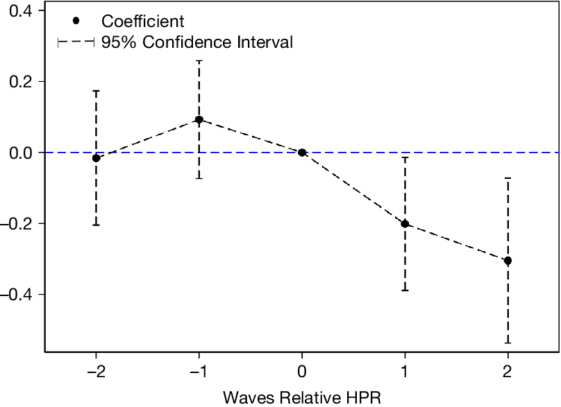
A basic condition of the DID method is the parallel trend assumption. We are concerned that if educational investment of households in surrounding unregulated cities has already shown a faster-declining trend than that of households in faraway cities before the implementation of the HPR policy, the negative effect estimated in the baseline regression may be overstated. In this section, we alleviate this concern by testing whether the parallel trends assumption is satisfied before the implementation of HPR. Specifically, we decompose the core explanatory variable, HPR_250 km, into a set of event-time indicators: Before 2, Before 1, After 1, and After 2, to study the dynamic impact on household educational investment. The regression model is specified as follows:

(2) $$ {Y}_{ijt}={\displaystyle \begin{array}{l}{\beta}_0+{\beta}_1 Before\hskip0.4em {2}_{jt}+{\beta}_2 Before\hskip0.4em {1}_{jt}+{\beta}_3 After\hskip0.4em {1}_{jt}+{\beta}_4 After\hskip0.4em {2}_{jt}\\ {}+\hskip2px {\beta}_5{X}_{ijt}+{\beta}_6{Z}_{jt}+{\gamma}_i+{\tau}_t+{\varepsilon}_{ijt},\end{array}} $$

where Before 2 (Before 1) is a dummy variable that equals 1 for households in the treatment group if the survey wave is two waves (one wave) before the implementation year of the HPR policy. After 2 (After 1) is a dummy variable that equals 1 for households in the treatment group if the survey wave is two waves (one wave) after the implementation year of the HPR policy.Footnote ⁵ The base group is the survey wave in the year of policy implementation.

Figure 1 plots the dynamic regression results. We notice that the coefficients of both Before 2 and Before 1 are not significant, indicating that there is no significant difference in household educational investment between the treatment and control groups before the event date. In contrast, the coefficients of After 1 and After 2 are significantly negative, suggesting that educational investment of households in nearby unregulated cities significantly decreases after the implementation of the restriction policy. This evidence validates the parallel trends assumption and ensures that our results are not driven by preexisting trends.

FIGURE 1Parallel Trends Test

Figure 1 shows the estimated coefficients and the 95% confidence intervals of a series of wave dummies for the survey waves before and after the HPR policy, estimated from specification (2). The base group is the survey wave in the implementation year of the HPR policy.

A line graph showing estimated coefficients and 95% confidence intervals across survey waves relative to the H P R policy. See long description.

FIGURE 1 Long description

A line graph with a horizontal x-axis labeled Waves Relative H P R and a vertical y-axis ranging from minus 0.4 to 0.4. A horizontal dashed blue line is fixed at 0.0 on the y-axis. The legend at the top left identifies black dots as Coefficient and dashed vertical bars as 95% Confidence Interval.

Moving from left to right along the x-axis.

* At wave minus 2, the coefficient is slightly below 0.0 with a wide confidence interval spanning from approximately minus 0.2 to 0.18.

* At wave minus 1, the coefficient rises to approximately 0.1 with a confidence interval from minus 0.05 to 0.25.

* At wave 0, the reference point, the coefficient is exactly 0.0 with no visible error bars.

* At wave 1, the coefficient drops to minus 0.2 with a confidence interval from minus 0.4 to 0.0.

* At wave 2, the coefficient further decreases to minus 0.3 with a confidence interval from minus 0.55 to minus 0.05.

The overall trend shows relatively stable pre-policy coefficients followed by a significant downward trajectory after the H P R policy implementation at wave 0.

2. Alternative Definitions of Treated Cities

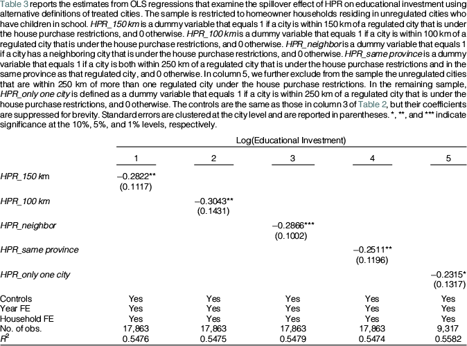
In the benchmark analysis, we define the treatment group as households in unregulated cities located within 250 km of regulated cities. To assess the robustness of our results, we consider five alternative definitions of treated cities. First, we reduce the spillover distance threshold from 250 to 150 km. Second, we further narrow this threshold to 100 km. Third, we use geographic adjacency and define an unregulated city as treated only if it is geographically bordering a regulated city. Fourth, we define an unregulated city as treated if it is both within 250 km of a regulated city and in the same province as that regulated city. Fifth, the treatment effect may be influenced by whether an unregulated city is located near one or multiple regulated cities, or by a change in the number of nearby regulated cities, such as a reduction from three to two. To ensure a cleaner identification of the effect, we conduct a subsample analysis focusing exclusively on treated cities that have only one nearby regulated city.

Table 3 reports the regression results from robustness tests using alternative definitions of HPR spillover. The coefficients of the core explanatory variables are negative and significant. Their magnitudes are consistent, falling within a narrow range of 23%–30%. This suggests that the results obtained from the baseline regressions are not sensitive to the specific choice of spillover distance. Moreover, the coefficient of interest is 28.22% for the 150 km threshold and 30.43% for the 100 km threshold, indicating that the spillover effect strengthens as the distance to regulated cities decreases.

TABLE 3Alternative Definitions of Treated Cities

A statistical table showing the impact of H P R on Log Educational Investment across five different city definitions. See long description.

TABLE 3 Long description

The table presents regression results for Log Educational Investment across five models.

Header: The columns are numbered 1 through 5.

Row 1: H P R underscore 150 k m. Column 1 shows minus 0.2822 with two asterisks and a standard error of 0.1117.

Row 2: H P R underscore 100 k m. Column 2 shows minus 0.3043 with two asterisks and a standard error of 0.1431.

Row 3: H P R underscore neighbor. Column 3 shows minus 0.2866 with three asterisks and a standard error of 0.1002.

Row 4: H P R underscore same province. Column 4 shows minus 0.2511 with two asterisks and a standard error of 0.1196.

Row 5: H P R underscore only one city. Column 5 shows minus 0.2315 with one asterisk and a standard error of 0.1317.

Fixed Effects and Controls: All five columns include Yes for Controls, Year F E, and Household F E.

Observations: Columns 1 through 4 have 17,863 observations. Column 5 has 9,317 observations.

R-squared: Values range from 0.5474 to 0.5582 across the five models.

3. Additional Control Variables

In this section, we test the robustness of the benchmark results by adding more control variables that may confound the spillover effect of HPR on the investment in children’s education. First, economic shocks to regulated cities might spill over to nearby unregulated cities, and the strength of this spillover effect could decrease with distance. Given this concern, we check whether our results are sensitive to the inclusion of the exposure of an unrelated city to the economic activity of the nearest regulated city. Specifically, for each unregulated city in our sample, we calculate the beta of its GDP growth to the nearest regulated city by using data from the year 2003 to the beginning of the sample period. We then compute the economic exposure of an unregulated city to the nearest regulated city as the corresponding beta times the regulated city’s GDP. Column 1 of Table 4 shows that the estimated effect of the HPR policy on educational investment hardly changes after controlling for intercity economic connections.

TABLE 4Additional Control Variables

A regression table showing the impact of additional control variables on Log Educational Investment across three models. See long description.

TABLE 4 Long description

The table presents regression results for Log Educational Investment across three columns labeled 1, 2, and 3.

* H P R _ 250 km: Column 1 shows minus 0.2307 with a standard error of 0.1006. Column 2 shows minus 0.3045 with a standard error of 0.1074. Column 3 shows minus 0.2520 with a standard error of 0.0909.

* Intercity economic connection: Column 1 shows 0.2428 with a standard error of 0.1888. Columns 2 and 3 are blank.

* C P I: Column 2 shows minus 0.0448 with a standard error of 0.0512. Columns 1 and 3 are blank.

* F I R E employment: Column 3 shows 0.2041 with a standard error of 0.1345. Columns 1 and 2 are blank.

* Construction employment: Column 3 shows minus 0.0265 with a standard error of 0.0934. Columns 1 and 2 are blank.

* Controls, Year F E, and Household F E: All three columns are marked Yes.

* Number of observations: Column 1 has 17,787. Column 2 has 14,615. Column 3 has 17,863.

* R-squared: Column 1 is 0.5464. Column 2 is 0.5399. Column 3 is 0.5478.

Second, higher house prices induced by the HPR policies may raise the cost of living for households in unregulated cities through inflation, thereby crowding out educational investment. To rule out this possibility, we incorporate city-level CPI data from the WIND database into the regression. Column 2 of Table 4 presents the results. We find that controlling for inflation does not alter the impact of HPR on educational investment.

Third, Charles et al. (Reference Charles, Hurst and Notowidigdo2018), who also study the nexus between the housing market and education, document that housing booms improve labor market opportunities, thereby lowering college enrollment. As such, it is possible that increased labor market opportunities make children less likely to go to college, thus leading to a decrease in educational investment. To account for this possibility, we obtain data on the city-level total employment in the finance, investment, and real estate (FIRE) sector and that in the construction sector from CSMAR, and additionally control for the natural logarithms of FIRE employment and construction employment. As shown in column 3 of Table 4, the inclusion of these two variables does not change our main findings, as the coefficient of HPR_250 km remains negative and statistically significant.

4. Heterogeneous Treatment Effects

Recent literature has shown that staggered DID regressions with two-way fixed effects may produce biased estimates if treatment effects are heterogeneous or if some comparisons receive negative weights (de Chaisemartin and D’Haultfoeuille (Reference de Chaisemartin and D’Haultfoeuille2023)). To address this concern, we perform a set of diagnostic tests. First, we employ the stacked DID approach developed by Cengiz, Dube, Lindner, and Zipperer (Reference Cengiz, Dube, Lindner and Zipperer2019), which estimates treatment effects by realigning cohorts at their treatment dates and stacking the resulting data sets. Specifically, for each HPR event, we include a clean control group and a treated group. The clean control group consists of household-year observations in cities that have not yet experienced any spillover effect from nearby HPR cities as of a given year, as well as households in cities that never experience any spillover effect during the sample period. We construct a cohort identifier and stack the cohort-specific data sets. This procedure eliminates biases from differential timing and heterogeneous effects, as suggested by Baker, Larcker, and Wang (Reference Baker, Larcker and Wang2022). Second, we reestimate the baseline regression using the DIDM estimator developed by de Chaisemartin and D’Haultfoeuille (Reference de Chaisemartin and D’Haultfoeuille2020), which is robust to treatment effect heterogeneity and avoids the negative weighting problem. Third, we apply the two-stage DID (DID2S) procedure proposed by Gardner (Reference Gardner2022), which partials out fixed effects in the first stage to correct for bias from differential treatment timing. Fourth, we drop the last period of the data of the panel data following recommendations from de Chaisemartin and D’Haultfoeuille (Reference de Chaisemartin and D’Haultfoeuille2023) and Jakiela (Reference Jakiela2021) and rerun the baseline DID regression to mitigate the potential influence of negative weights.

Table 5 reports the results of these diagnostic tests. We find that the impact of HPR on educational investment remains robustly negative and significant. The point estimates under stacked DID, DIDM, and DID2S are similar to our baseline estimate, and with the final period removed, the estimated treatment effect is virtually unchanged. Overall, these findings confirm the robustness of our findings.

TABLE 5Diagnostic Tests for Heterogeneous Treatment Effects

A statistical table showing diagnostic tests for heterogeneous treatment effects on Log Educational Investment using four different models. See long description.

TABLE 5 Long description

The table compares four models: Stacked D I D (Column 1), D I D M (Column 2), D I D 2 S (Column 3), and Excluding the Last Wave (Column 4).

* The primary variable H P R underscore 250 km shows negative coefficients across all models:

- Stacked D I D: minus 0.2873 with a standard error of 0.0942.

- D I D M: minus 0.2077 with a standard error of 0.0935.

- D I D 2 S: minus 0.2108 with a standard error of 0.0695.

- Excluding the Last Wave: minus 0.2435 with a standard error of 0.0827.

* Controls are marked as ‘Yes’ for all four columns.

* Fixed Effects (F E) vary by model:

- Stacked D I D uses Year cross cohort F E and Household cross cohort F E.

- The other three models use Year F E and Household F E.

* Sample size and R-squared:

- Number of observations: 48,589 (Col 1), 9,604 (Col 2), 15,420 (Col 3), and 14,140 (Col 4).

- R-squared: 0.5794 (Col 1) and 0.5597 (Col 4). Values for Col 2 and 3 are not provided.

V. Further Analysis

A. Mechanism Analysis: Evidence of Housing Speculation

We contend that the negative effect of the HPR policy on educational investment of families in surrounding unregulated cities is likely driven by a substitution effect between housing and educational investment. Deng et al. (Reference Deng, Liao, Yu and Zhang2022) document that the HPR policy in regulated cities creates a positive spillover effect, triggering a sharp rise in housing prices in adjacent unregulated cities. As suggested by Gao et al. (Reference Gao, Sockin and Xiong2020) and Mian and Sufi (Reference Mian and Sufi2022), a sharp increase in house prices alters price growth expectations among potential buyers and fuels speculative activity. In this context, we hypothesize that rising house prices in nearby unregulated cities lead households to anticipate further appreciation. When expected returns on housing investment rise, households may reallocate funds toward real estate, thereby crowding out educational expenditure due to extrapolative expectations in the housing market. Overall, the HPR policy stimulates housing speculation in surrounding unregulated cities and reduces investment in children’s education. This crowding-out effect could be especially pronounced in China, both because Chinese households lack formal investment channels and real estate investment serves as a major investment vehicle, and because educational expenses are nontrivial in China. Under a fixed budget constraint, housing and educational investments are to some extent substitutes. To verify this housing speculation channel, we conduct several tests as follows.

1. House Prices and Attention to Housing Market

The key assumption regarding the negative impact of the HPR policy on educational investment by families in nearby unregulated cities lies in its positive shock to the real estate market in those cities. Therefore, we first need to verify whether the HPR policy produces a positive spillover effect on housing prices in surrounding unregulated cities.

High-quality house price data are not easily accessible in China, especially for medium and small cities. For example, the National Bureau of Statistics (NBS) in China provides a house price index based on the average selling price of newly built housing units, which ignores transactions of existing properties and fails to control for housing quality (Wu, Gyourko, and Deng (Reference Wu, Gyourko and Deng2012), Fang et al. (Reference Fang, Gu, Xiong and Zhou2016)). To tackle this issue, we obtain a house price index from CityRE, a leading real estate data provider in China. CityRE constructs a constant-quality hedonic house price index using listing and transaction data from national and local real estate brokers, covering more than 300 cities in China. The quality of the CityRE index has been well recognized in recent studies (e.g., Deng et al. (Reference Deng, Liao, Yu and Zhang2022), Ma and Zhang (Reference Ma and Zhang2024)).

We now use the natural logarithm of the annual house price index as the dependent variable and report the results in column 1 of Table 6. HPR_250 km enters positively and significantly in the regression, confirming a positive spillover effect of the HPR policy on the real estate market in surrounding unregulated cities. In economic terms, the estimated coefficient of 0.1102 implies that house prices in nearby unregulated cities increase by 11.02% relative to the control group after the HPR policy.

TABLE 6House Prices and Attention to Housing Markets

A regression table showing the relationship between house prices and housing market attention across three models. See long description.

TABLE 6 Long description

The table consists of three columns representing different dependent variables: 1 Log House Price Index, 2 Log Search for House Price, and 3 Log Search for House Purchase.

* The primary independent variable is H P R sub 250 km.

* For Model 1, the coefficient is 0.1102 with a standard error of 0.0243.

* For Model 2, the coefficient is 0.1254 with a standard error of 0.0369.

* For Model 3, the coefficient is 0.1181 with a standard error of 0.0361.

* All three coefficients are statistically significant at the 1 percent level, indicated by three asterisks.

* All models include Controls, Year F E, and City F E.

* Number of observations are 2,133 for Model 1, and 2,219 for Models 2 and 3.

* R-squared values are 0.9373 for Model 1, 0.9005 for Model 2, and 0.9088 for Model 3.

Next, we check whether the positive impact of the HPR policy on the real estate market in surrounding unregulated cities heightens household attention to these markets. We use data from Baidu, the largest search engine in China. Baidu provides an index, similar to Google Trends, called the Baidu Index, which measures the search intensity of specific keywords (Vaughan and Chen (Reference Vaughan and Chen2015)). Using this tool, we construct a city-level search index based on keywords related to the housing market (e.g., “house price” and “house purchase”). This index serves as the dependent variable to capture the impact of the HPR policy on housing market attention in surrounding unregulated cities.

Columns 2 and 3 in Table 6 present the results. The positive coefficients of HPR_250 km in the two regressions indicate that the HPR policy significantly increases search volumes for terms such as “house price” and “house purchase” among households in surrounding unregulated cities relative to those in farther unregulated cities. In terms of economic magnitude, the estimated coefficients of HPR_250 km are 0.1254 and 0.1181, which imply that the HPR policy raises search volumes for “house price” and “house purchase” by 12.54% and 11.81%, respectively, in nearby unregulated cities. Therefore, the HPR policy and the ensuing house price surge significantly elevate housing-related attention among households in these cities, providing strong support for the housing speculation channel.

2. House Price Expectation and House Purchase Intention

We have found that the HPR policy indeed had a spillover effect on the real estate market in surrounding unregulated cities, not only driving up house prices but also significantly increasing attention to the housing market in these cities. To further validate the housing speculation channel, we examine households’ subjective assessment of the housing market and their intentions to invest in housing. Specifically, we construct two dummy variables based on the CHFS questionnaire. House price expectation is a dummy variable that equals 1 if the respondent expects house prices to rise in the next 3 months, and 0 otherwise. House purchase intention is a dummy variable that equals 1 if the respondent has a plan to invest in a house, and 0 otherwise. We rerun regressions with these two variables as the dependent variables, respectively.

Table 7 reports the impact of the HPR policy on house price expectations and house purchase intentions of families in surrounding unregulated cities versus those in faraway unregulated cities. Note that the question about house price expectations was only asked in 2011 and 2019, and the question about house purchase intention has some missing values. Therefore, the number of observations in Table 7 is smaller than those in the benchmark regressions.Footnote ⁶ As shown in column 1 of Table 7, the coefficient of HPR_250 km is significantly positive, indicating that households living in nearby unregulated cities and experiencing the house price boom are more likely to have positive expectations of future house price growth than those located in faraway cities. The positive coefficient of interest in column 2 of Table 7 further shows that the HPR policy significantly increases the intentions of families in surrounding unregulated cities to purchase a house. These results demonstrate that the introduction of the HPR policy strengthens households’ expectations of future house price growth and their intentions to invest in the housing market in those cities, which corroborates the housing speculation hypothesis.

TABLE 7House Price Expectation and House Purchase Intention

A statistical table showing the relationship between house price expectations and purchase intentions across two models. See long description.

TABLE 7 Long description

The table consists of three columns. The first column lists variables and fixed effects, while columns 1 and 2 represent House Price Expectation and House Purchase Intention respectively.

* Row 1, H P R _ 250 km: Column 1 shows 0.1642 with three asterisks and a standard error of 0.0357. Column 2 shows 0.0584 with two asterisks and a standard error of 0.0230.

* Row 2, Controls: Both columns are marked Yes.

* Row 3, Year F E: Both columns are marked Yes.

* Row 4, City F E: Column 1 is Yes, Column 2 is No.

* Row 5, Household F E: Column 1 is No, Column 2 is Yes.

* Row 6, Number of observations: Column 1 has 2,814. Column 2 has 12,789.

* Row 7, R-squared: Column 1 is 0.0660. Column 2 is 0.5096.

3. Reallocation of Household Resources

The speculative demand for housing investment may crowd out not only educational expenditures but also other categories of household consumption and investments in alternative assets. In other words, the HPR policy may induce a broader reallocation of household resources. To test this conjecture, we first consider two other types of expenditures, namely basic expenditure and discretionary expenditure. The former covers necessities such as food, clothing, and commuting, while the latter includes nonessential items like entertainment and travel. Panel A of Table 8 shows the regression results using the logarithms of basic and discretionary expenditures as dependent variables. While basic consumption shows no significant change, households in treated cities significantly reduce discretionary spending by 13.69% following the HPR policy. This distinction may be attributed to the downward rigidity in adjusting basic consumption.

TABLE 8Reallocation of Household Resources

A two-panel regression table showing the impact of H P R underscore 250 km on household expenditure and portfolio choices. See long description.

TABLE 8 Long description

The table is divided into two sections.

Panel A, Other Expenditure Categories, examines Log Basic Expenditure in column 1 and Log Discretionary Expenditure in column 2. For H P R underscore 250 km, the coefficient for Basic Expenditure is 0.0374 with a standard error of 0.0241. The coefficient for Discretionary Expenditure is negative 0.1369 with two asterisks, indicating statistical significance, and a standard error of 0.0588. Both models include Controls, Year F E, and Household F E. The number of observations is 17,863. The R-squared values are 0.7266 and 0.6550 respectively.

Panel B, Portfolio Choice, examines Stock Ownership in column 1 and Stock Share in column 2. For H P R underscore 250 km, the coefficient for Stock Ownership is negative 0.0252 with three asterisks and a standard error of 0.0089. The coefficient for Stock Share is negative 0.0085 with one asterisk and a standard error of 0.0046. Both models include Controls, Year F E, and Household F E. The number of observations is 12,666. The R-squared values are 0.7449 and 0.6162 respectively.

We next probe whether treated households rebalance their portfolios in response to the HPR shock, focusing on household stock market participation. Following the literature (e.g., Malmendier and Nagel (Reference Malmendier and Nagel2011), Giannetti and Wang (Reference Giannetti and Wang2016)), we employ two measures: Stock ownership, a dummy variable indicating whether the household owns stocks directly or indirectly through mutual funds, and Stock share, the fraction of household wealth invested in stocks. These two measures capture the extensive and intensive margins of stock market participation, respectively.

Panel B of Table 8 presents the results for household portfolio choice. The coefficient of HPR_250 km is negative and significant in both regressions, indicating that households in treated cities significantly reduce stock investment after the HPR shock. In terms of economic magnitude, the HPR policy reduces the probability of stock ownership by 2.52 percentage points and the proportion of household wealth allocated to stocks by 0.85 percentage points relative to distant unregulated cities. These findings support the argument that housing booms resulting from the HPR spillovers dampen the attractiveness of other investment opportunities relative to real estate.

4. Reasons for Needing Funds

To provide more direct evidence of the crowding-out effects of housing speculation, we examine changes in households’ reported reasons for needing funds around the policy shock. In principle, if the story of housing speculation holds, households should substitute housing investment for educational investment. Consequently, we would expect them to be more likely to report needing funds for housing investment and less likely to report needing funds for education.

We utilize a two-step set of questions regarding household credit demand to test our conjecture. In the first step, respondents are asked: “Does your household currently need funds?” If the response is “Yes,” a follow-up question is presented: “What is the primary reason your household needs funds?” Response options include “for house purchase,” “for health expenses,” “for children’s education,” “for financial investment,” “for automobile purchase,” “for gifts and ceremony,” and “for basic living expenses.” We restrict our analysis to households responding “Yes” in the first step. Specifically, we construct two dummy variables: For house purchase, which indicates whether the primary reason for needing funds is house purchase, and For children’s education, which indicates whether the primary reason is children’s education. Using the same DID approach as in our benchmark analysis, we examine the impact of HPR on households’ stated reasons for needing funds.Footnote ⁷ Table 9 shows the regression results. We observe that households in nearby unregulated cities become more likely to need funds for house purchase and less likely to need them for children’s education after the implementation of the HPR policy. This finding bolsters our conjecture regarding the housing speculation channel.

TABLE 9Reasons for Needing Funds

A statistical table showing regression results for two reasons for needing funds: house purchase and children's education. See long description.

TABLE 9 Long description

The table consists of three columns. The first column lists variables and diagnostics, while columns 1 and 2 represent the dependent variables: For House Purchase and For Children’s Education.

* Row 1: H P R _ 250 km. For House Purchase, the coefficient is 0.0370 double asterisk with a standard error of 0.0183. For Children’s Education, the coefficient is minus 0.0388 double asterisk with a standard error of 0.0175.

* Row 2: Controls. Both columns indicate Yes.

* Row 3: Year F E. Both columns indicate Yes.

* Row 4: City F E. Both columns indicate Yes.

* Row 5: Number of observations. Both columns show 8,257.

* Row 6: R super 2. For House Purchase, the value is 0.1072. For Children’s Education, the value is 0.1842.

5. Parental Aspirations for Children’s Education

When parents perceive the opportunity to earn “easy money” through speculation during a housing boom, their subjective belief in the importance of education may weaken. Accordingly, they may adjust their aspirations for children’s education. This shift has important long-term implications, as parental aspirations play a critical role in determining children’s educational outcomes (Hao and Yeung (Reference Hao and Yeung2015)).

To shed light on the spillover effect of the HPR policy on parental aspirations for children’s education, we turn to another data set, the China Family Panel Studies (CFPS), as the CHFS does not collect information on educational aspirations. The CFPS is a large-scale survey conducted by the Institute of Social Science Survey (ISSS) at Peking University in collaboration with the Survey Research Center at the University of Michigan. The CFPS data have been increasingly used in the literature to study household behaviors in China (e.g., Huang and Zhang (Reference Huang and Zhang2021)). We use waves from 2010 to 2020 to construct an unbalanced panel.

We measure aspirations for children’s education using the survey question “What is the highest education level you would like your child to achieve?” Based on this question, we construct a variable, Aspirations for children’s education, which represents the number of years of schooling that parents desire for their children. Then, we run a regression of this variable using the same specification as in the benchmark analysis. Table 10 reports the regression results. We find that the HPR policy significantly reduces the educational aspirations of parents living in nearby unregulated cities. Specifically, we estimate that parents’ desired years of schooling for their children in treated cities fall by about 0.29 years, or approximately 3–4 months, on average. Relative to the sample mean of 14.62 years, which corresponds to a college degree, this decline is small (about 2% of the mean). When standardized by the sample standard deviation (2.76 years), the effect amounts to approximately 10% of the standard deviation. While modest, this effect is nonnegligible, especially considering that parental educational aspirations are typically highly stable and exhibit limited variation over time (Schörner and Bittmann (Reference Schörner and Bittmann2024)). Thus, even a small estimated effect may reflect a meaningful shift in parental expectations. Most importantly, the significantly negative effect is informative: it suggests that parents are unlikely to view housing primarily as a savings vehicle to finance future education. If that channel were dominant, one would expect desired years of schooling to increase, not decrease. This evidence appears consistent with the conjecture that the perceived opportunities to profit from housing speculation may weaken parents’ belief in the value of education.

TABLE 10Parental Aspirations for Children’s Education

A statistical table showing the negative impact of H P R 250 km on parental aspirations for children's education. See long description.

TABLE 10 Long description

The table consists of two columns. The first column lists the variables and the second column provides the corresponding values for Aspirations for Children’s Education.

* Row 1: H P R underscore 250 km has a coefficient of minus 0.2864 with two asterisks indicating statistical significance.

* Row 2: The standard error for the coefficient is 0.1213.

* Row 3: Controls are marked as Yes.

* Row 4: Year F E is marked as Yes.

* Row 5: Household F E is marked as Yes.

* Row 6: Number of observations is 18,869.

* Row 7: R super 2 value is 0.4641.

B. Heterogeneity Analyses

We conduct three heterogeneity analyses to further reveal the substitution effect between housing investment and educational investment. First, we consider whether the effect differs across families with different levels of education and wealth. More educated individuals may place more weight on educational investment and be less affected by the speculative demand for housing investment. Hence, we hypothesize that the HPR effect is weaker for households with higher educational attainment. In addition, because financially constrained families are more likely to substitute housing investment with educational investment, we expect the HPR effect to be attenuated by the wealth level. Accordingly, we construct two dummy variables. High education is a dummy variable that equals 1 if the respondent’s years of schooling are above the sample median, and 0 otherwise. High household wealth is a dummy variable that equals 1 if the household’s total wealth is above the sample median, and 0 otherwise. To account for potential correlation between these two variables, we include both wealth and education in the same regression. Specifically, we add two interaction terms: one between HPR_250 km and High education, and another between HPR_250 km and High household wealth, while controlling for both main effects. Column 1 of Table 11 reports the results. We find that the coefficients of both interaction terms are significantly positive. Hence, consistent with our conjecture, the crowding-out effects of housing investment on educational investment are weaker for families with higher levels of wealth and those with higher levels of education. The heterogeneity across wealth levels further suggests that easing borrowing constraints may help mitigate the crowding-out effect of housing speculation, as wealthier households are generally less financially constrained.

TABLE 11Heterogeneity Analyses

A statistical table showing heterogeneity analyses for Log Educational Investment across three models. See long description.

TABLE 11 Long description

The table presents regression results for Log Educational Investment across three columns labeled 1, 2, and 3.

Row 1: H P R _ 250 km. Column 1: minus 0.5379 with three asterisks (standard error 0.1124). Column 2: minus 0.2889 with two asterisks (standard error 0.1204). Column 3: minus 0.2239 with one asterisk (standard error 0.1294).

Row 2: H P R _ 250 km times high education. Column 1: 0.2710 with one asterisk (standard error 0.1373).

Row 3: H P R _ 250 km times high household wealth. Column 1: 0.4009 with three asterisks (standard error 0.0826).

Row 4: H P R _ 250 km times primary or secondary school. Column 2: 0.0697 (standard error 0.1118).

Row 5: H P R _ 250 km times college. Column 2: 0.2478 (standard error 0.2050).

Row 6: H P R _ 250 km times homebuyer. Column 3: minus 0.1684 with two asterisks (standard error 0.0742).

Fixed Effects and Statistics:

- Controls: Yes for all columns.

- Year F E: Yes for all columns.

- Household F E: Yes for all columns.

- Number of observations: 17,863 for Column 1; 13,298 for Column 2; 17,863 for Column 3.

- R super 2: 0.5508 for Column 1; 0.5523 for Column 2; 0.5482 for Column 3.

Second, an alternative interpretation of our results is that households may be speculating in housing as a means to save for their children’s college expenses, intending to sell properties later to fund education. In other words, they may view housing investment as an optimal savings vehicle during a housing boom. If this is the case, we expect the HPR effects to be weaker for households with children in university.

To test this savings vehicle hypothesis, we examine whether the spillover effect of HPR on educational investment varies across children’s age groups. Specifically, we create two dummy variables: one indicating whether the household has a child in primary or secondary school (Primary and secondary school), and another indicating whether the household has a child in university (College). Households with children in kindergarten serve as the base group. Then, we interact HPR_250 km with these two dummy variables and exclude households with children spanning multiple age groups to ensure clear comparability. As shown in column 2 of Table 11, both interaction terms are statistically insignificant, suggesting that the HPR effects do not differ significantly across children’s age groups. This finding to some extent contradicts the savings-for-college interpretation, as the HPR effects remain significant even among households with children in university. In addition, this result indicates that increased labor market opportunities cannot fully explain our results, as the crowding-out effects persist even in households with children who are not of working age.

Third, if the HPR policy indeed leads households to prioritize housing investment over education spending, its impact should be stronger among those who actually purchased a home after the policy implementation compared to those who did not. To test this conjecture, we define a dummy variable, Homebuyer, which equals 1 if the respondent purchased a home after the HPR policy shock, and 0 otherwise. We then incorporate an interaction term between HPR_250 km and Homebuyer into the regression model. The results, presented in column 3 of Table 11, show a significantly negative coefficient of the interaction term. This supports our hypothesis, indicating that the effects of the HPR policy are stronger among households that acquired additional property following the policy shock.

C. Comparing Single-Home and Multiple-Home Owners

The impact of rising housing prices on consumption may vary across households with different homeownership status. For example, multiple-home owners are more likely to benefit from the wealth effect of rising house prices. To capture this heterogeneity, we conduct subsample analyses that distinguish between single-home households and multiple-home owners. Table 12 reports OLS estimates examining differential spillover effects of HPR on three expenditure categories across single-home and multiple-home owners. The results show that HPR significantly reduces educational investment and discretionary consumption among single-home households. By contrast, the effects for multiple-home owners turn positive, though statistically insignificant. These findings suggest that the speculative effect of HPR on education spending is driven primarily by single-home owners. This heterogeneity suggests that the relative strength of the speculative and wealth effects of housing booms varies across households with different homeownership statuses.

TABLE 12Comparing Single-Home and Multiple-Home Owners

A regression table comparing single-home and multiple-home owners across three expenditure categories. See long description.

TABLE 12 Long description

A data table with seven columns. The first column lists variables, while the remaining six columns are grouped into three pairs representing Log Educational Investment, Log Basic Expenditure, and Log Discretionary Expenditure. Each pair compares Single-Home owners with Multiple-Home owners.

* Row 1, H P R underscore 250 km:

- Log Educational Investment: Single-Home -0.2604 (significant at 5 percent level), Multiple-Home 0.0565.

- Log Basic Expenditure: Single-Home 0.0385, Multiple-Home 0.0607.

- Log Discretionary Expenditure: Single-Home -0.1228 (significant at 5 percent level), Multiple-Home 0.0376.

* Row 2, Standard Errors:

- Log Educational Investment: Single-Home 0.1276, Multiple-Home 0.1679.

- Log Basic Expenditure: Single-Home 0.0253, Multiple-Home 0.0443.

- Log Discretionary Expenditure: Single-Home 0.0624, Multiple-Home 0.0849.

* Row 3, Controls: Yes for all columns.

* Row 4, Year F E: Yes for all columns.

* Row 5, Household F E: Yes for all columns.

* Row 6, Number of observations: Single-Home columns have 14,150; Multiple-Home columns have 3,713.

* Row 7, R-squared: Values range from 0.5144 to 0.7280 across the models.

Using automobile sales data, Deng et al. (Reference Deng, Liao, Yu and Zhang2022) find that the HPR policy increases automobile consumption. The difference between their results and ours may be partly attributable to heterogeneous responses across household types, as documented in our study, as well as to the characteristics of automobile consumption in China. Vehicle ownership per capita in China was 0.19 in 2020 (Duan et al. (Reference Duan, Song, Wang, Jian, Heijungs and Chen2024)), indicating that a considerable proportion of households do not own a car. For these households, automobile spending is effectively censored at zero and therefore has no scope for further decline. In addition, automobile purchasers in China tend to be substantially wealthier than the average population (Grier et al. (Reference Grier, Hicks and Yuan2016)). As a result, automobile sales data in China are likely to capture a selective sample of relatively wealthier households. Moreover, wealthier households tend to have higher automobile consumption, so their consumption behavior could exert a greater influence on city-level automobile sales examined in Deng et al. (Reference Deng, Liao, Yu and Zhang2022). Meanwhile, wealthier households are more likely to own more housing assets and thus experience stronger wealth effects from rising housing prices. Overall, the positive effects documented in Deng et al. (Reference Deng, Liao, Yu and Zhang2022) may disproportionately reflect the consumption responses of households in the relatively right-hand tail of the wealth distribution, who are more likely to benefit from increases in housing prices. Consequently, rising house prices might simultaneously induce cutbacks in education spending among many homeowners in our household-level data, while increasing aggregate automobile consumption driven by wealthier homeowners in city-level sales data.

VI. Welfare Implications

An important question is how our findings affect individual and social welfare. While a precise answer is beyond this article’s scope, we outline some plausible implications.

First, we calculate the Sharpe ratio (defined as the mean divided by the standard deviation) of the housing price growth rate and our results indicate that the Sharpe ratio for treated cities during this period is 1.0989, suggesting that housing investments in these cities generate a positive risk-adjusted return ex post.

However, individual investors may not necessarily realize positive capital gains if they did not sell at the appropriate time; without realized sales, appreciation does not translate into realized returns. China’s housing market slowed sharply after our sample period, with Bank of International Settlements (BIS) data showing a 20% decline in residential housing prices between 2021:Q3 and 2024:Q4. In light of the subsequent downturn, households in nearby unregulated cities were unlikely to realize capital gains unless they sold their properties in a timely manner. In fact, data in our sample suggest that few households sold their properties after the HPR shock, reflecting China’s prevalent buy-and-hold strategy (Glaeser et al. (Reference Glaeser, Huang, Ma and Shleifer2017)). This tendency is reinforced by the lack of recurrent property tax, higher levies on short-term property sales, and prolonged boom-driven beliefs in ever-rising prices. Thus, households in treated cities appear unlikely to have possessed superior information and may ultimately have been unable to realize capital gains.

Second, rational investment involves diversification. Excessive allocation to real estate amplifies portfolio risk, a concern especially relevant in China where housing constitutes about 60% of household assets (Li, Li, Lu, and Xie (Reference Li, Li, Lu and Xie2020)) and most sampled households already own homes.

Third, even if housing investment ultimately pays off for some households, its impact on future educational spending remains uncertain. The perceived prospect of making fortunes through speculation may weaken parents’ beliefs in the importance of education, and the success in speculation could further strengthen such beliefs.

Fourth, educational investment is cumulative, with early inputs enhancing the returns to later ones (Cunha, Heckman, Lochner, and Masterov (Reference Cunha, Heckman, Lochner and Masterov2006)). Insufficient investment at critical stages can cause lasting harm to human capital (Attanasio, Meghir, and Nix (Reference Attanasio, Meghir and Nix2020)). Therefore, a reduction in current educational investment induced by housing speculation might cause an irreversible welfare loss for the household in the long run.

Fifth, shifting investment from human capital to housing may be socially suboptimal. Consistent with evidence on resource misallocation in housing booms (Chen and Wen (Reference Chen and Wen2017), Charles et al. (Reference Charles, Hurst and Notowidigdo2018)), our findings suggest that by crowding out education, speculation might lower aggregate human capital and, in turn, long-run productivity and growth.

VII. Conclusion

This article explores the impact of the spillover effect of the HPR policy on educational investment in nearby unregulated cities. After controlling for household and city characteristics, we find that compared with faraway unregulated cities, the HPR policy significantly reduces the educational investment of families in nearby unregulated cities. Our additional analyses reinforce the housing speculation channel. Following the HPR policy shock, house prices, market attention, and expectations of future price growth rise in nearby unregulated cities, while discretionary consumption, stock investment, and educational aspirations fall. These phenomena are consistent with households reallocating resources toward housing. Heterogeneity tests show that the HPR effect is stronger for less wealthy and less educated households, persists across children’s age groups, and is more pronounced among households that acquired additional property. Finally, the crowding-out effect is concentrated among single-home households, rather than those owning multiple homes.

Our article provides a new perspective on the real impact of housing market dynamics: housing speculation, resulting from a rapid and dramatic increase in house prices, may increase the relative attractiveness of housing investment and crowd out other investments, particularly those that only pay off in the very long run. The speculation channel differs from but complements the wealth effect and collateral effect of housing booms documented in existing studies. As education is the main driver of long-term growth and development, while real estate booms might stimulate local economies in the short run, the induced housing speculation may, to some extent, lead to distortions in capital allocation and welfare losses in the long run.

Government interventions in housing markets are not unique to China. Our results suggest that transaction restrictions and related policies can have spillover effects on household decisions beyond housing itself, which warrant attention from policymakers and researchers. The extent and direction of these spillovers are likely to depend on institutional characteristics. We acknowledge that our estimates are identified in, and perhaps amplified by, China’s institutional context, where access to home-equity extraction is limited, capital markets are relatively underdeveloped, and a prolonged housing fever has occurred. As such, the magnitudes we report should not be directly extrapolated to other economies. A productive direction for future work is to test the substitution effect we propose in settings with different housing market characteristics, financial infrastructures, and policy instruments.

Finally, our study focuses on a relatively short-term span after the HPR policy shock. When more long-term data become available, it would be interesting to explore the long-term effects on households’ wealth accumulation, children’s educational outcomes, and their labor market performance.

Supplementary Material

To view supplementary material for this article, please visit http://doi.org/10.1017/S0022109026102713.

Funding Statement

Niu acknowledges the financial support received from the National Natural Science Foundation of China (Grant No. 72573125) and the Humanities and Social Science Foundation of the Ministry of Education of China (Grant No. 23XJC790005). Zhou acknowledges the financial support received from the National Natural Science Foundation of China (Grant No. 72273098), the Humanities and Social Science Foundation of the Ministry of Education of China (Grant No. 21YJC790172), and the Fundamental Research Funds for the Central Universities (Grant No. 413000439).

Footnotes

We thank an anonymous referee, Xu Gan, Weijie Lu, Yuan Ren, Zhao Rong, Stephan Siegel (the editor), Bo Zhang, Yapei Zhang, and Yunqi Zhang for their helpful comments.

¹ Land price changes are calculated based on the constant quality land price index for 35 major markets in China created by Wu et al. (Reference Wu, Gyourko and Deng2012), namely the Wharton/NUS/Tsinghua Chinese Residential Land Price Indexes (CRLPI). House price changes are calculated based on the constant quality house price index for major cities in China constructed by Fang et al. (Reference Fang, Gu, Xiong and Zhou2016).

² Note that our measure of educational investment does not include savings for children’s future education.

³ We adopt time-invariant inclusion rules at the household level. Specifically, to maintain consistency, each household’s homeownership status, including whether they are renters or multiple homeowners, is determined according to their status in the first survey wave they participated in. This classification might include households that later sell their homes and become renters. Such cases constitute only a small fraction of the sample, and excluding them does not materially alter our results.

⁴ Residential mobility in China is relatively low due to a strong culture of hometown preference and the household registration system that creates barriers to settling permanently outside one’s city of registration (Song (Reference Song2014)). Moreover, our sample consists exclusively of homeowners with children, who should face higher moving costs and thus tend to exhibit particularly low mobility over short periods. In line with this, we find that approximately 99% of households in the CHFS data stay in the same city between consecutive survey waves. This figure is consistent with the findings in other studies using China’s household survey data (e.g., Deschenes, Wang, Wang, and Zhang (Reference Deschenes, Wang, Wang and Zhang2020), Li, Ferreira, Smith, and Zhang (Reference Li, Ferreira, Smith and Zhang2021)).

⁵ Note that the relatively short time span of the sample prevents us from estimating leads and lags of three periods or more for all treated cities.

⁶ We have to replace household fixed effects with city fixed effects in the regression of house price expectations due to the lack of household-level panel data for this specific question.

⁷ Note that because this two-step question covers a subsample of households with very limited overlap across panel waves, we have to replace household fixed effects with city fixed effects.

References

Adelino, M.; Schoar, A.; and Severino, F.. “House Prices, Collateral and Self-Employment.” Journal of Financial Economics, 117 (2015), 288–306.CrossRef Google Scholar

Agarwal, S., and Qian, W.. “Access to Home Equity and Consumption: Evidence from a Policy Experiment.” Review of Economics and Statistics, 99 (2017), 40–52.CrossRef Google Scholar

Aghion, P., and Howitt, P.. The Economics of Growth. Cambridge, MA: MIT Press (2008).Google Scholar

Armona, L.; Fuster, A.; and Zafar, B.. “Home Price Expectations and Behaviour: Evidence from a Randomized Information Experiment.” Review of Economic Studies, 86 (2019), 1371–1410.CrossRef Google Scholar

Attanasio, O.; Meghir, C.; and Nix, E.. “Human Capital Development and Parental Investment in India.” Review of Economic Studies, 87 (2020), 2511–2541.CrossRef Google Scholar

Baker, A. C.; Larcker, D. F.; and Wang, C. C.. “How Much Should We Trust Staggered Difference-in-Differences Estimates?” Journal of Financial Economics, 144 (2022), 370–395.CrossRef Google Scholar

Becker, G. S. Human Capital and the Personal Distribution of Income. Ann Arbor, MI: University of Michigan Press (1967).Google Scholar

Cengiz, D.; Dube, A.; Lindner, A.; and Zipperer, B.. “The Effect of Minimum Wages on Low-Wage Jobs.” Quarterly Journal of Economics, 134 (2019), 1405–1454.CrossRef Google Scholar

Charles, K. K.; Hurst, E.; and Notowidigdo, M. J.. “Housing Booms and Busts, Labor Market Opportunities, and College Attendance.” American Economic Review, 108 (2018), 2947–2994.CrossRef Google Scholar

Chen, K.; Wang, Q.; Xu, T.; and Zha, T.. “Impacts of LTV Policy on the Mortgage Market via Housing Speculation.” Working Paper, Emory University (2022).Google Scholar

Chen, K., and Wen, Y.. “The Great Housing Boom of China.” American Economic Journal: Macroeconomics, 9 (2017), 73–114.Google Scholar

Chen, Y. J.; Chen, Z.; and He, S.. “Social Norms and Household Savings Rates in China.” Review of Finance, 23 (2019), 961–991.CrossRef Google Scholar

Chen, Y. Y.; Yuan, M.; and Zhang, M.. “Income Inequality and Educational Expenditures on Children: Evidence from the China Family Panel Studies.” China Economic Review, 78 (2023), 101932.CrossRef Google Scholar

Corradin, S., and Popov, A.. “House Prices, Home Equity Borrowing, and Entrepreneurship.” Review of Financial Studies, 28 (2015), 2399–2428.CrossRef Google Scholar

Cunha, F.; Heckman, J. J.; Lochner, L.; and Masterov, D. V.. “Interpreting the Evidence on Life Cycle Skill Formation.” Handbook of the Economics of Education, 1 (2006), 697–812.Google Scholar

de Chaisemartin, C., and D’Haultfoeuille, X.. “Two-Way Fixed Effects Estimators with Heterogeneous Treatment Effects.” American Economic Review, 110 (2020), 2964–2996.CrossRef Google Scholar

de Chaisemartin, C., and D’Haultfoeuille, X.. “Two-Way Fixed Effects and Differences-in-Differences with Heterogeneous Treatment Effects: A Survey.” The Econometrics Journal, 26 (2023), C1–C30.CrossRef Google Scholar

Deng, Y.; Liao, L.; Yu, J.; and Zhang, Y.. “Capital Spillover, House Prices, and Consumer Spending: Quasi-Experimental Evidence from House Purchase Restrictions.” Review of Financial Studies, 35 (2022), 3060–3099.CrossRef Google Scholar

Deschenes, O.; Wang, H.; Wang, S.; and Zhang, P.. “The Effect of Air Pollution on Body Weight and Obesity: Evidence from China.” Journal of Development Economics, 145 (2020), 102461.CrossRef Google Scholar

Disney, R., and Gathergood, J.. “House Prices, Wealth Effects and Labour Supply.” Economica, 85 (2018), 449–478.CrossRef Google Scholar

Duan, L.; Song, L.; Wang, W.; Jian, X.; Heijungs, R.; and Chen, W. Q.. “Urbanization Inequality: Evidence from Vehicle Ownership in Chinese Cities.” Humanities and Social Sciences Communications, 11 (2024), 1–12.CrossRef Google Scholar

Fan, G.; Li, H.; Li, J.; and Zhang, J.. “Housing Property Rights, Collateral, and Entrepreneurship: Evidence from China.” Journal of Banking and Finance, 143 (2022), 106588.CrossRef Google Scholar

Fang, H.; Gu, Q.; Xiong, W.; and Zhou, L. A.. “Demystifying the Chinese Housing Boom.” NBER Macroeconomics Annual, 30 (2016), 105–166.CrossRef Google Scholar

Fu, Y.; Qian, W.; and Yeung, B.. “Speculative Investors and Transactions Tax: Evidence from the Housing Market.” Management Science, 62 (2016), 3254–3270.CrossRef Google Scholar

Gan, J. “Housing Wealth and Consumption Growth: Evidence from a Large Panel of Households.” Review of Financial Studies, 23 (2010), 2229–2267.CrossRef Google Scholar

Gao, Z.; Sockin, M.; and Xiong, W.. “Economic Consequences of Housing Speculation.” Review of Financial Studies, 33 (2020), 5248–5287.CrossRef Google Scholar

Gardner, J. “Two-Stage Differences in Differences.” arXiv preprint, arXiv:2207.05943 (2022).Google Scholar

Giannetti, M., and Wang, T. Y.. “Corporate Scandals and Household Stock Market Participation.” Journal of Finance, 71 (2016), 2591–2636.CrossRef Google Scholar

Glaeser, E. L., and Nathanson, C. G.. “An Extrapolative Model of House Price Dynamics.” Journal of Financial Economics, 126 (2017), 147–170.CrossRef Google Scholar

Glaeser, E. L.; Huang, W.; Ma, Y.; and Shleifer, A. V.. “A Real Estate Boom with Chinese Characteristics.” Journal of Economic Perspectives, 31 (2017), 93–116.CrossRef Google Scholar

Glancy, D. “Housing Bust, Bank Lending and Employment: Evidence from Multimarket Banks.” Journal of Banking and Finance, 127 (2021), 106111.CrossRef Google Scholar

Grier, K. B.; Hicks, D. L.; and Yuan, W.. “Marriage Market Matching and Conspicuous Consumption in China.” Economic Inquiry, 54 (2016), 1251–1262.CrossRef Google Scholar

Han, B.; Han, L.; and Zhu, G.. “Housing Price and Fundamentals in a Transition Economy: The Case of the Beijing Market.” International Economic Review, 59 (2018), 1653–1677.CrossRef Google Scholar

Han, L.; Lutz, C.; Sand, B. M.; and Stacey, D. G.. “The Effects of a Targeted Financial Constraint on the Housing Market.” Review of Financial Studies, 34 (2021), 3742–3788.CrossRef Google Scholar

Hanushek, E. A.; Kinne, L.; Lergetporer, P.; and Woessmann, L.. “Patience, Risk-Taking, and Human Capital Investment Across Countries.” Economic Journal, 132 (2021), 2290–2307.CrossRef Google Scholar

Hao, L., and Yeung, W. J. J.. “Parental Spending on School-Age Children: Structural Stratification and Parental Expectation.” Demography, 52 (2015), 835–860.CrossRef Google Scholar PubMed

Huang, W., and Zhang, C.. “The Power of Social Pensions: Evidence from China’s New Rural Pension Scheme.” American Economic Journal: Applied Economics, 13 (2021), 179–205.Google Scholar

Jakiela, P. “Simple Diagnostics for Two-Way Fixed Effects.” arXiv preprint, arXiv:2103.13229 (2021).CrossRef Google Scholar

Jia, N.; Zhou, Y.; and Yang, T.. “‘Selective Two–Child’ Policy and Household Resource Allocation.” China Economic Review, 68 (2021), 101639.CrossRef Google Scholar

Johnson, W. R. “House Prices and Female Labor Force Participation.” Journal of Urban Economics, 82 (2014), 1–11.CrossRef Google Scholar

Johnson, R. C. “The Impact of Parental Wealth on College Degree Attainment: Evidence from the Housing Boom and Bust.” AEA Papers and Proceedings, 110 (2020), 405–410.CrossRef Google Scholar

Kartashova, K., and Tomlin, B.. “House Prices, Consumption and the Role of Non-Mortgage Debt.” Journal of Banking and Finance, 83 (2017), 121–134.CrossRef Google Scholar

Kuchler, T.; Piazzesi, M.; and Stroebel, J.. “Housing Market Expectations.” In Handbook of Economic Expectations, Bachmann, R., Topa, G., and van der Klaauw, W., eds. Amsterdam, Netherlands: Elsevier (2023), 163–191.CrossRef Google Scholar

Li, H.; Li, J.; Lu, Y.; and Xie, H.. “Housing Wealth and Labor Supply: Evidence from a Regression Discontinuity Design.” Journal of Public Economics, 183 (2020), 104139.CrossRef Google Scholar

Li, M.; Ferreira, S.; Smith, T. A.; and Zhang, X.. “Air Pollution and Noncognitive Traits among Chinese Adolescents.” Health Economics, 30 (2021), 478–488.CrossRef Google Scholar PubMed

Liang, P., and Guo, S.. “Social Interaction, Internet Access and Stock Market Participation—An Empirical Study in China.” Journal of Comparative Economics, 43 (2015), 883–901.CrossRef Google Scholar

Liu, C., and Xiong, W.. “China’s Real Estate Market.” In Handbook of China’s Financial System, Amstad, M., Sun, G., and Xiong, W., eds. Princeton, NJ: Princeton University Press (2020), 181–207.Google Scholar

Lovenheim, M. F. “The Effect of Liquid Housing Wealth on College Enrollment.” Journal of Labor Economics, 29 (2011), 741–771.CrossRef Google Scholar

Lovenheim, M. F., and Reynolds, C. L.. “The Effect of Housing Wealth on College Choice: Evidence from the Housing Boom.” Journal of Human Resources, 48 (2013), 1–35.CrossRef Google Scholar

Ma, C., and Zhang, S.. “Can Housing Booms Elevate Financing Costs of Financial Institutions?” Journal of Development Economics, 167 (2024), 103230.CrossRef Google Scholar

Malmendier, U., and Nagel, S.. “Depression Babies: Do Macroeconomic Experiences Affect Risk Taking?” Quarterly Journal of Economics, 126 (2011), 373–416.CrossRef Google Scholar

Mian, A. R., and Sufi, A.. “Credit Supply and Housing Speculation.” Review of Financial Studies, 35 (2022), 680–719.CrossRef Google Scholar

Mian, A. R.; Rao, K.; and Sufi, A.. “Household Balance Sheets, Consumption, and the Economic Slump.” Quarterly Journal of Economics, 128 (2013), 1687–1726.CrossRef Google Scholar

Mian, A. R.; Sufi, A.; and Trebbi, F.. “Foreclosures, House Prices, and the Real Economy.” Journal of Finance, 70 (2015), 2587–2634.CrossRef Google Scholar

Musso, A.; Neri, S.; and Stracca, L.. “Housing, Consumption and Monetary Policy: How Different Are the US and the Euro Area?” Journal of Banking and Finance, 35 (2011), 3019–3041.CrossRef Google Scholar

Painter, G.; Yang, X.; and Zhong, N.. “Housing Wealth as Precautionary Saving: Evidence from Urban China.” Journal of Financial and Quantitative Analysis, 57 (2022), 761–789.CrossRef Google Scholar

Oreopoulos, P., and Salvanes, K. G.. “Priceless: The Nonpecuniary Benefits of Schooling.” Journal of Economic Perspectives, 25 (2011), 159–184.CrossRef Google Scholar

Schmalz, M. C.; Sraer, D. A.; and Thesmar, D.. “Housing Collateral and Entrepreneurship.” Journal of Finance, 72 (2017), 99–132.CrossRef Google Scholar

Schörner, K., and Bittmann, F.. “Children’s Aspirations, Their Perceptions of Parental Aspirations, and Parents’ Factual Aspirations—Gaining Insights into a Complex World of Interdependencies.” European Sociological Review, 40 (2024), 981–995.CrossRef Google Scholar

Song, Y. “What Should Economists Know About the Current Chinese Hukou System?” China Economic Review, 29 (2014), 200–212.CrossRef Google Scholar

Tian, X., and Wang, Y.. “Housing Speculation and Entrepreneurship.” Review of Finance (2025), rfaf056.Google Scholar

Vaughan, L., and Chen, Y.. “Data Mining from Web Search Queries: A Comparison of Google Trends and Baidu Index.” Journal of the Association for Information Science and Technology, 66 (2015), 13–22.CrossRef Google Scholar

Wang, H.; Cheng, Z.; and Smyth, R.. “Parental Misbeliefs and Household Investment in Children’s Education.” Economics of Education Review, 89 (2022), 1–15.CrossRef Google Scholar

Wu, J.; Gyourko, J.; and Deng, Y.. “Evaluating Conditions in Major Chinese Housing Markets.” Regional Science and Urban Economics, 42 (2012), 531–543.CrossRef Google Scholar

Xu, H. “Physical and Mental Health of Chinese Grandparents Caring for Grandchildren and Great-Grandparents.” Social Science and Medicine, 229 (2019), 106–116.CrossRef Google Scholar PubMed

Zhao, L., and Burge, G.. “Housing Wealth, Property Taxes, and Labor Supply Among the Elderly.” Journal of Labor Economics, 35 (2017), 227–263.CrossRef Google Scholar

TABLE 1Summary StatisticsTABLE 1 Long description.

TABLE 2Benchmark ResultsTABLE 2 Long description.

FIGURE 1Parallel Trends TestFigure 1 shows the estimated coefficients and the 95% confidence intervals of a series of wave dummies for the survey waves before and after the HPR policy, estimated from specification (2). The base group is the survey wave in the implementation year of the HPR policy.FIGURE 1 Long description.