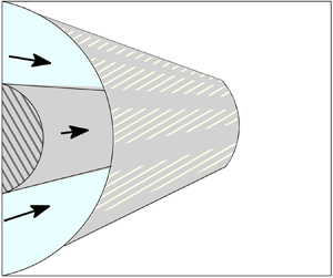

1. Introduction
This paper has been inspired by a recent investigation of the effects of geometry on coaxial pipe flows (Williams et al. Reference Williams, Turney, Moulton and Waters2020). Such flows are ubiquitous in a range of applications from oil recovery to healthcare. Williams et al. (Reference Williams, Turney, Moulton and Waters2020) refer to a surgical biomedical tool called a ureteroscope which exploits a coaxial pipe flow in the laminar regime to treat kidney stones. It is an externally operated device requiring the delivery and return of fluid into a patient but at controllable flow rates and with strong physiological constraints for its safe operation on the allowable pressure gradients driving the flow. Consequently, Williams et al. (Reference Williams, Turney, Moulton and Waters2020) explored the design options based on changing the geometry of both the inner and outer tube boundaries in order to maximize the volume flux while minimizing the driving pressure gradient.
A quite different physical mechanism for drag reduction in pressure-driven internal flows of this kind – one that that is of topical interest and used most commonly in micro- and nano-fluidics – is superhydrophobicity of the confining walls. Superhydrophobic surfaces rely on the presence of free surface menisci spanning surface protrusions in the microstructure that furnish boundary regions that are close to being free of shear and thereby allow slip (Rothstein Reference Rothstein2010). The regime where such spanning menisci between surface protrusions exist is called the Cassie state and stands in contrast to the Wenzel state where the surface is fully wetted. A review with a good survey of relevant references has been given by Lee, Choi & Kim (Reference Lee, Choi and Kim2016).
One challenge of significant recent interest is the quantification of the effective slip length associated with flows involving superhydrophobic surfaces of this mixed no-slip/no-shear type. Theoretically, this is a homogenization problem where one seeks to capture the global effect on slip of the microstructural details of the surface by modelling a superhydrophobic wall by an effective Navier-slip boundary condition of the form
 \begin{equation} \lambda \frac{\partial w }{\partial n} = w, \end{equation}
where  $\lambda$ is the Navier-slip length parameter,
 $w(x,y)$ is the longitudinal flow along a pipe with a cross-section in the
 $(x,y)$ plane and
 $\partial /\partial n$ denotes the inward normal derivative in this cross-plane. The question then becomes: how does the effective slip length
 $\lambda$ depend on details of the surface microstructure?
The study of textured surfaces to reduce friction most commonly occurs in confined internal channel flows that are relatively easy to set up in a laboratory setting. However, pipe flow has also received some attention. Watanabe, Udagawa & Udagawa (Reference Watanabe, Udagawa and Udagawa1999) studied experimentally the effect of superhydrophobic walls on flow in a single-walled pipe and achieved a reduction in drag of up to 14 % in the laminar regime compared to a fully no-slip scenario. Further studies into drag reduction, this time in low-pressure driven flows in copper mesh pipes with internal hydrophobic walls were carried out by Shirtcliffe et al. (Reference Shirtcliffe, McHale, Newton and Zhang2009) with more recent work contributed by Walker et al. (Reference Walker, Albadarin, McGlue, Brennan and Bell2014). On a practical level significant challenges remain in designing and building effective pipes with superhydrophobic walls although some recent progress has been made by Geraldi et al. (Reference Geraldi, Dodd, Xu, Wells, Newton and McHale2017). While the reduction of hydrodynamic friction is of interest for a wide range of applications, there are also design challenges in other applications such as heat transfer. Lv & Zhang (Reference Lv and Zhang2016) recently looked at a double-tube heat exchanger and studied the interplay between hydrodynamic friction reduction and heat transfer effects in a flow scenario where fluid is travelling both in the central pipe and the annular pipe region exterior to that pipe and an external wall.
The contribution of the present paper is theoretical. It follows in the spirit of an important paper by Philip (Reference Philip1972) which has, by now, become a standard theoretical reference in the burgeoning field of surface engineering. Although it was not concerned with superhydrophobicity per se, Philip's paper records analytical solutions to a range of canonical mixed boundary value problems comprising a mixture of no-shear and no-slip boundaries. Those canonical problems are relevant to modelling superhydrophobic surfaces with the no-shear boundaries serving as a good first model of the spanning menisci in the Cassie state, especially when the viscosity of the fluid trapped in the grooves is much lower than that of the working fluid (Asmolov & Vinogradova Reference Asmolov and Vinogradova2012; Schönecker & Hardt Reference Schönecker and Hardt2013; Crowdy Reference Crowdy2017c). The larger question of the relevance of this no-shear assumption in practice is a topic of active discussion (Crowdy Reference Crowdy2017b).
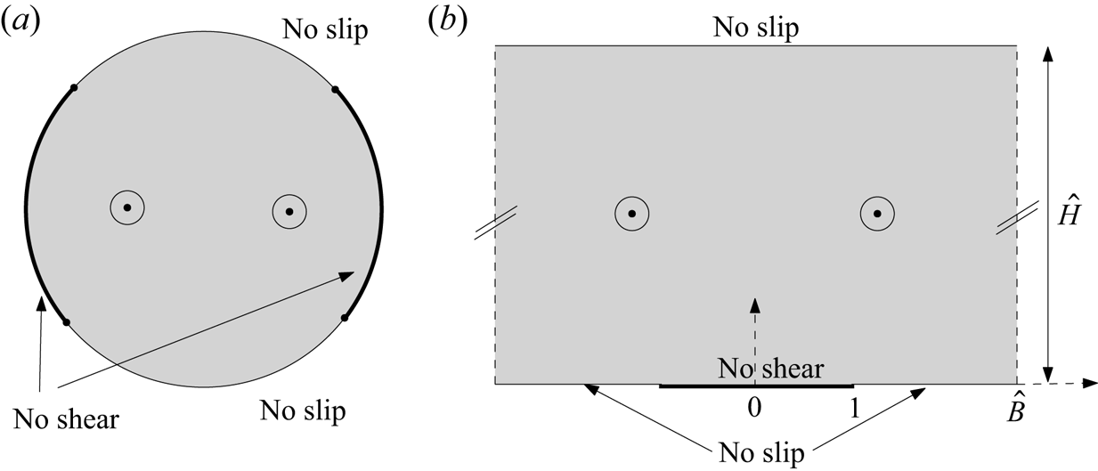
One of Philip's solutions describes longitudinal flow along a single-walled pipe with a rotationally symmetric pattern of  $N$ no-shear grooves running along its length where
 $N \ge 1$ is an integer as shown in cross-section in figure 1 in the case
 $N=2$. We will refer to this as Philip's pipe flow solution; he presents it in terms of trigonometric functions. Another solution, involving two walls, is for flow in a channel with a periodic array of no-shear grooves on the lower wall and no-slip imposed on the upper wall; we will refer to this as Philip's channel flow solution. Philip presents it in terms of the Jacobi cnoidal function. Figure 1 shows a cross-section of a typical period window of such a flow.
Two problems solved by Philip (Reference Philip1972): his longitudinal pipe flow solution (a) and his channel flow solution (b) with a periodic array of no shear slots on the lower wall (single period window shown). Off the no-shear slots, shown as bold line segments, the no-slip condition holds. Cross-sections are shown with longitudinal flow into the page.

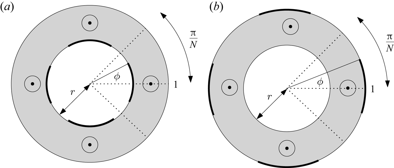
As extensions of Philip's work, and motivated in part by the annular pipe flow investigations of Williams et al. (Reference Williams, Turney, Moulton and Waters2020), solutions for the following flow scenarios would appear to be of interest: longitudinal superhydrophobic annular pipe flow – or what we will call an ‘annular SH pipe’ – with one no-slip wall and another decorated with a rotationally symmetric pattern of  $N \ge 1$ no-shear grooves running along its length. Such solutions are not given by Philip (Reference Philip1972) and are derived here. These flows are natural generalizations of his pipe flow and channel flow solutions just discussed as will be seen. Figure 2 shows cross-sections of the two annular SH pipe flows we have in mind: longitudinal no-shear slots are either on the inner or the outer wall of the pipe, but not both. The latter possibility is discussed in § 8.
The annular superhydrophobic pipes (‘annular SH pipes’) of interest here:  $N$ no-shear slots on the inner boundary wall (a) or the outer boundary wall (b). The case
 $N=4$ is shown. Off the no-shear slots, shown as bold line segments, the no-slip condition holds. Cross-sections are shown with longitudinal flow into the page.

Like Philip's, the new annular SH pipe solutions will be derived using complex analysis and conformal mapping techniques. The flows give rise to mixed boundary value problems for Poisson's equation that are not conformally invariant, and there appears to be no easy way to simply transform Philip's existing channel flow solution to provide the sought-after annular SH pipe solutions. Moreover, even if such a transformation was identified, Philip's channel flow solution is expressed in terms of the Jacobi cnoidal function, and its inverse, for complex-valued arguments. Those are recognized special functions but they are not particularly well known to applied scientists and actually not so easy to evaluate.
Philip (Reference Philip1972) uses the Schwarz–Christoffel formula to find many of his solutions but he omits the details. We will deploy a different mathematical strategy making use of a special transcendental function called the prime function associated with a concentric annulus (Crowdy Reference Crowdy2020). Not only does the method furnish the new solutions, but it has the bonus of providing alternative representations of Philip's two solutions in figure 1. There are analytical connections between these various solutions. The new method produces all of them from the same series of arguments and clarifies the connections.
Incidentally, the author (Crowdy Reference Crowdy2011a) has previously shown how to use this prime function to both re-express and generalize some other solutions found in Philip (Reference Philip1972) for both longitudinal and transverse shear flow over a periodic array of flat no-shear slots. This generalization is to the case where each period window contains not just one but any number of flat no-shear slots. A recent monograph (Crowdy Reference Crowdy2020) surveys other applications of the prime function in fluid mechanics and beyond.
It is useful to summarize the main results, not least for the benefit of readers who might wish to use them, or their associated effective slip lengths, without being concerned with their derivation.
Let the velocity field have the form 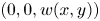 $(0,0,w(x,y))$ in Cartesian coordinates
 $(x,y,Z)$ where the cross-sectional plane is the
 $(x,y)$ plane and
 $Z$ is the longitudinal coordinate. Such a flow associated with the two annular SH pipes shown in figure 2, with outer radius set to unity and inner radius
 $r$, has axial velocity given by
 \begin{equation} w(x,y)= \frac{1 -z \bar{z} }{4} + \frac{1 }{2} \textrm{Re} \left [ h(z) \right ],\quad z=x+\textrm{i} y. \end{equation}
All that differs between the solutions for the two cases in figure 2 is the functional form of the analytic function  $h(z)$.
Patterning on inner wall: When the patterning comprises  $N \ge 1$ no-shear slots on the inner wall the function
 $h(z)$ is defined by
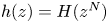 $h(z) = H(z^N)$ where
 \begin{equation} H(\zeta) = \frac{1 }{N} \int^\zeta_{-1} \left \lbrace r^2 - R \left [ \frac{P(\zeta'/q,q) P(\zeta'/q,q) }{P(\zeta'/a,q) P(\zeta'/\bar{a},q)}\right ]^{1/2} \right \rbrace \frac{\textrm{d} \zeta' }{\zeta'},\quad q=r^N,\enspace a = q\,\textrm{e}^{\textrm{i} \theta},\end{equation}
with the constant  $R$ calculated from formula (3.21a,b) recorded later. The angle
 $\theta = N \phi$, where the angle
 $\phi$ is the half-angle subtended at the centre of the pipe by a typical no-shear slot as shown in figure 2. It is a measure of the no-shear fraction, indeed
 $\theta /{\rm \pi}$ is the proportion of the total surface occupied by the no-shear zones. The special function
 $P(\zeta ,q)$, which is essentially the prime function for the concentric annulus (Crowdy Reference Crowdy2020), can be defined for any
 $\zeta \ne 0$ by the convergent infinite product
 \begin{equation} P(\zeta,q) \equiv (1-\zeta) \prod_{n=1}^\infty (1-q^{2n} \zeta)(1-q^{2n} /\zeta),\quad 0 \le q < 1. \end{equation}
The effective slip length associated with this flow – to be defined in § 2 – is
 \begin{equation} \lambda = r \log r - 2 r \left \lbrace \frac{\displaystyle{\frac{1 }{2N} \int^{-q}_{-1} \left [ \frac{P(\zeta/q,q) P(\zeta/q,q) }{P(\zeta/a,q) P(\zeta/\bar{a},q)} \right ]^{1/2} \frac{\textrm{d}\zeta }{\zeta}} }{\displaystyle{\frac{1 }{2 {\rm \pi}\textrm{i}} \oint_{C} \left [ \frac{P(\zeta/q,q) P(\zeta/q,q) }{P(\zeta/a,q) P(\zeta/\bar{a},q)} \right ]^{1/2} \frac{\textrm{d}\zeta }{\zeta}} } \right \rbrace, \end{equation}
where  $C$ is any closed circle inside the annulus
 $q < |\zeta | < 1$ and enclosing the origin.
Patterning on outer wall: When the patterning is on the outer wall 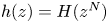 $h(z) = H(z^N)$ is now given by the modified form
 \begin{equation} H(\zeta) = \frac{1 }{N} \int^\zeta_{-1} \left \lbrace 1 - R \left [ \frac{P(\zeta',q) P(\zeta',q) }{P(\zeta'/a,q) P(\zeta'/\bar{a},q)} \right ]^{1/2} \right \rbrace \frac{\textrm{d} \zeta' }{\zeta'},\quad q=r^N,\enspace a = \textrm{e}^{\textrm{i} \theta}. \end{equation}
Again  $\theta = N \phi$, where the angle
 $\phi$ is shown in figure 2. The value of
 $R$ is now different and is given by formula (4.3a,b). The effective slip length associated with this flow is
 \begin{equation} \lambda = \log r - 2 \left \lbrace \frac{ \displaystyle{\frac{1 }{2N} \int^{-q}_{-1} \left [ \frac{P(\zeta,q) P(\zeta,q) }{P(\zeta/a,q) P(\zeta/\bar{a},q)} \right ]^{1/2} \frac{\textrm{d} \zeta }{\zeta}} }{\displaystyle{\frac{1 }{2 {\rm \pi}\textrm{i}} \oint_{C} \left [ \frac{P(\zeta,q) P(\zeta,q) }{P(\zeta/a,q) P(\zeta/\bar{a},q)} \right ]^{1/2} \frac{\textrm{d} \zeta }{\zeta}} } \right \rbrace, \end{equation}
where  $C$ is any closed circle inside the annulus
 $q < |\zeta | < 1$ and enclosing the origin.
The expressions (1.3) and (1.6) require a quadrature, but they are nevertheless explicit, and the quadrature is easily performed to high accuracy using standard integration routines. More will be said about this later.
As for new representations of Philip's two solutions shown in figure 1, his pipe flow solution is simply the  $r \to 0$ limit of (1.2) with
 $h(z)$ defined in (1.6) yielding
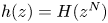 $h(z) = H(z^N)$ where, in this limit,
 \begin{equation} H(\zeta) \to \frac{1 }{N} \int^\zeta_{-1} \left \lbrace 1 - {\left (\frac{(1-\zeta')(1-\zeta') }{(1-\zeta'/a) (1-\zeta'/\bar{a})} \right )^{1/2}} \right \rbrace \frac{\textrm{d} \zeta' }{\zeta'},\quad a = \textrm{e}^{\textrm{i} \theta}, \end{equation}
as discussed in § 5. The associated slip length  $\lambda _P^{(\,{pipe})}$ is given by
 \begin{equation} \lambda_P^{({pipe})} = H(0) = \frac{1 }{N} \int^0_{-1} \left \lbrace 1 - {\left (\frac{(1-\zeta)(1-\zeta) }{(1-\zeta/a) (1-\zeta/\bar{a})} \right )^{1/2}} \right \rbrace \frac{\textrm{d} \zeta }{\zeta} = \frac{2 }{N} \log \sec(\theta/2),\end{equation}
where the last equality follows from a standard calculus exercise. This form of the solution avoids the trigonometric  $\cos$ and
 $\cos ^{-1}$ functions used by Philip (Reference Philip1972) although those formulas follow from (1.8) as confirmed in appendix C. Since it avoids the multi-valuedness of inverse trigonometric functions it is our view that (1.8) is easier to use in practice and more illuminating in theory.
In a similar way it will be shown that Philip's channel flow solution has the alternative form
 \begin{equation} w(x,y)= - \frac{y^2 }{2} + \frac{{\hat H} }{2}\textrm{Re}[H(\textrm{e}^{\textrm{i} {\rm \pi}z/\hat B})], \end{equation}
where the geometrical parameters  $\hat B$ and
 $\hat H$ are shown in figure 1 and
 \begin{equation} H(\zeta) = {\mathcal{R}} \int^\zeta_{-1} \left [ \frac{P(\zeta',\rho) P(\zeta',\rho) }{P(\zeta'/c,\rho) P(\zeta'/\bar{c},\rho)}\right ]^{1/2} \frac{\textrm{d} \zeta' }{\zeta'},\quad c=\textrm{e}^{\textrm{i} {\rm \pi}/\hat B},\enspace \rho = \textrm{e}^{-{\rm \pi} \hat H/\hat B}, \end{equation}
where the constant  ${\mathcal {R}}$ is now given in (6.4a,b). A convenient expression for the effective slip length
 $\lambda _P^{(channel)}$ associated with Philip's channel flow solution is
 \begin{equation} \lambda_P^{({channel})} = - \hat H - \frac{\hat B }{\rm \pi} \left \lbrace \frac{ \displaystyle{\int_{-1}^{-\rho} \left [ \frac{P(\zeta,\rho) P(\zeta,\rho) }{P(\zeta/c,\rho) P(\zeta/\bar{c},\rho)} \right ]^{1/2} \frac{\textrm{d} \zeta }{\zeta}} }{\displaystyle{ \frac{1 }{2 {\rm \pi}\textrm{i}} \oint_{C} \left [ \frac{P(\zeta,\rho) P(\zeta,\rho) }{P(\zeta/c,\rho) P(\zeta/\bar{c},\rho)} \right ]^{1/2} \frac{\textrm{d} \zeta }{\zeta} }}\right \rbrace, \end{equation}
where  $C$ is any closed circle in the annulus
 $\rho < |\zeta | < 1$ and enclosing the origin. Formula (1.12) contains only a ratio of non-singular integrals that can be evaluated using standard quadrature techniques. Philip (Reference Philip1972) does not include an expression for this effective slip length. Just as no
 $\cos$ and
 $\cos ^{-1}$ functions appear in (1.2) and (1.8), no Jacobi
 $\textrm {cn}$ and
 $\textrm {cn}^{-1}$ functions appear in (1.10)–(1.11). Appendix D connects (1.10)–(1.11) to Philip's solution. A link to elliptic functions emerges because the prime function (1.4) is related, after a change of variables, to the first Jacobi theta function (Crowdy Reference Crowdy2020).
Formulas (1.10)–(1.11) which involve an indefinite integral are no less explicit than Philip's solution given in terms of  $\textrm {cn}$ and
 $\textrm {cn}^{-1}$ since those functions are themselves usually calculated, in special function packages, using integral representations. Rather, formulas (1.10)–(1.11) make any such integrals explicit and tangible for ready calculation, and without the need for special function packages. Our new forms of Philip's solutions also have theoretical value in clarifying how the new annular SH pipe solutions, with
 $H(\zeta )$ given by (1.3) and (1.6), are generalizations of Philip's solutions where the relevant
 $H(\zeta )$ is either (1.8) for his pipe flow solution or (1.11) for his channel flow solution.
The structure of the paper is as follows. In § 2 the mixed boundary value problems are formulated and the effective slip length defined. Section 3 presents in detail the derivation of the solution (1.2)–(1.3) for the case of no-shear patterning on the inner wall. In § 4 the analogous solution for no-shear patterning on the outer wall is written down and the slip properties analysed. Sections 5 and 6 show how the two solutions of Philip (Reference Philip1972) fit into this mathematical framework. In § 7 all the solutions are characterized and their friction properties, as encoded by the effective slip lengths, are calculated, analysed and compared. A final section discusses future implications of the theoretical results.
2. Mixed-type boundary value problem and the effective slip length
Pressure-driven longitudinal flow 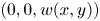 $(0,0,w(x,y))$ of a fluid of viscosity
 $\mu$ along a uniform pipe having a cross-section in the
 $(x,y)$ plane is governed by
 \begin{equation} \nabla^2 w = -\frac{s }{\mu},\quad \nabla^2 = \frac{\partial^2 }{\partial x^2} + \frac{\partial^2 }{\partial y^2}, \end{equation}
where  $-s$ is the pressure gradient along the axis of the pipe. The focus here is on concentric annular pipes with an inner and an outer circular wall; see figure 2. Lengths are non-dimensionalized with respect to the outer-wall radius
 $R_0$ and the velocity with respect to
 $s R_0^2/\mu$ meaning that we must solve the non-dimensionalized version of (2.1a,b) in the domain
 $r < |z| < 1$ where
 $z=x+\textrm {i} y$ and
 $r$ is the ratio of inner and outer radii of the annular pipe. The forcing on the right-hand side of (2.1a,b) then becomes
 $-1$.
The boundary condition will be taken to be one of two types: either a no-slip condition  $w=0$ on any portion of solid wall, or a no-shear condition
 ${\partial w/\partial n}=0$ on any meniscus where
 $\partial /\partial n$ denotes the inward normal derivative to the fluid region. Mixed boundary value problems involve combinations of these conditions on the same boundary. It is this mixture of conditions that makes these boundary value problems challenging. Singularities of the shear stress must be expected at the points on any boundary where the boundary condition changes type and they must be resolved carefully. Such singularities can cause accuracy and convergence problems in numerical approaches to solving this class of problems rendering the availability of analytical solutions all the more valuable, not least as checks on numerical codes.
Once a flow is set up to quantify the hydrodynamic slip it is usual to define a so-called effective slip length which involves equating the total volume flux caused by a given pressure gradient to that associated with a suitable comparison flow. Several definitions are possible and we will explain our choice. Suppose the outer wall of the annular pipe contains the rotationally symmetric pattern of no-shear slots and suppose the associated flow 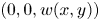 $(0,0,w(x,y))$ has a volume flux
 ${\mathcal {Q}}$ defined by
 \begin{equation} {\mathcal{Q}} = \int \int_{r <|z| < 1} w(x,y)\,\textrm{d}\kern0.7pt x\,\textrm{d} y. \end{equation}
On the outer surface  $|z|=1$ a mixture of no-slip and no-shear boundary conditions is imposed, and
 $|z|=r$ is a no-slip surface. It is convenient to replace this set of mixed conditions on
 $|z|=1$ by a single Navier-slip boundary condition
 \begin{equation} \lambda \frac{\partial w_{NS} }{\partial n} = w_{NS},\quad |z|=1, \end{equation}
containing the slip length parameter  $\lambda$. Our choice is to retain the boundary condition on the inner boundary
 $|z|=r$ as being one of no slip. The driving pressure gradient for this ‘comparison flow’
 $(0,0,w_{NS}(x,y))$ is taken to be unchanged. Such a flow in this geometry and with these boundary conditions will be axisymmetric. Suppose its associated volume flux is
 \begin{equation} {Q} = \int \int_{r <|z| < 1} w_{NS}(x,y)\,\textrm{d}\kern0.7pt x\,\textrm{d} y. \end{equation}
The effective slip length for the original annular SH pipe is defined to be the value of  $\lambda$ for which
 $Q = {\mathcal {Q}}$.
The most general axisymmetric solution of the non-dimensionalized partial differential equation (2.1a,b) is
 \begin{equation} w_{NS}(x,y) = \frac{1 -|z|^2 }{4} + A \log |z| + B,\quad z=x+\textrm{i} y, \end{equation}
for some constants  $A$ and
 $B$. Such a solution depends only on the radial distance
 $|z|$. If
 $|z|=r$ is a no-slip wall then
 \begin{equation} 0 = \frac{1 -r^2 }{4} + A \log r + B. \end{equation}
The associated volume flux is defined by
 \begin{equation} Q = \int \int_{r <|z| < 1} w_{NS}(x,y)\,\textrm{d}\kern0.7pt x\,\textrm{d} y \equiv {\mathcal{F}}(A,B;r) \end{equation}
and the function  ${\mathcal {F}}(A,B;r)$ can be readily calculated. It is unnecessary to do so, however, to compute the effective slip length due to the following mathematical observations.
First it is easy to show that  $\lambda$ is related to the parameters
 $A$ and
 $B$ from the axisymmetric flow solution via
 \begin{equation} \lambda = \frac{2 B }{1- 2A}. \end{equation}
In the other case, where a no-slip condition holds on  $|z|=1$ and the Navier-slip condition (2.3a,b) holds on the inner wall, the corresponding relation is
 \begin{equation} \lambda = \frac{r }{2} \left [ \frac{1-r^2 + 4 A \log r + 4B }{2 A - r^2} \right ]. \end{equation}
For the flow in the annular SH pipe with no shear slots on the outer wall the solution will have the more general form
 \begin{equation} w(x,y) = \frac{1 -z \bar{z} }{4} + \frac{1 }{2} \textrm{Re}[h(z)], \end{equation}
where  $h(z)$ is an analytic function in the annulus
 $r < |z| < 1$. It is not necessarily single valued though. Its real part is, however, single valued and this constrains
 $h(z)$ to have a representation, convergent in the annulus, of the form
 \begin{equation} h(z) = {\mathcal{A}} \log z + {\mathcal{B}} + \sum_{n \ge 1}\left [ {h_n z^n} + \frac{h_{-n} r^n }{z^n} \right ] \end{equation}
for some  ${\mathcal {A}}, {\mathcal {B}} \in \mathbb {R}$ and a set of coefficients
 $\lbrace h_n, h_{-n} \in \mathbb {C} |n = 1,2, \ldots \rbrace$ that will be determined by the boundary conditions. If the inner wall
 $|z|=r$ is a no-slip wall with no boundary point singularities then the representation (2.11) remains convergent and the boundary condition there implies
 \begin{equation} 0 = \frac{1 - r^2 }{4} + \frac{1 }{2} ({\mathcal{A}} \log r + {\mathcal{B}}) + \frac{1 }{4} \sum_{n \ge 1} \left [ {(h_n +\overline{h_{-n}} r^{-n}) z^n} + \frac{r^n }{z^n} (h_{-n}+r^n \overline{h_n})\right ]. \end{equation}
On equating coefficients of powers of  $z$ we must have
 \begin{equation} h_{-n}+r^n \overline{h_n}= 0,\quad n = 1,2, \ldots \end{equation}
and
 \begin{equation} 0 = \frac{1 - r^2 }{4} + \frac{1 }{2} ({\mathcal{A}} \log r + {\mathcal{B}}). \end{equation}
The latter is exactly the same relation (2.6) as that between  $A$ and
 $B$ in the axisymmetric solution (2.5).
At the same time it is easy to demonstrate, using the complex form of Stokes theorem, that the contribution to the volume flux  ${\mathcal {Q}}$ defined in (2.2) from each term in
 $w(x,y)$ of the form
 \begin{equation} \textrm{Re} \left [ {h_n z^n} + \frac{h_{-n} r^n }{z^n} \right ],\quad n \ge 1 \end{equation}
is identically zero; see appendix A. This means that the volume flux  ${\mathcal {Q}}$ associated with this more general non-axisymmetric flow is given by
 \begin{equation} {\mathcal{Q}} = {\mathcal{F}}({\mathcal{A}},{\mathcal{B}};r), \end{equation}
where  ${\mathcal {F}}$ is defined in (2.7) as the flux associated with the axisymmetric flow. On combining the two observations (2.14) and (2.16) the effective slip length as defined earlier is inferred to be
 \begin{equation} \lambda = \frac{2 {\mathcal{B}} }{1- 2{\mathcal{A}}}= \frac{2{\mathcal{A}} \log r + 1 -r^2 }{2 {\mathcal{A}}-1}. \end{equation}
Therefore, to compute the effective slip length  $\lambda$ we need only find the parameter
 ${\mathcal {A}}$ and there is no need to compute any volume fluxes.
By similar arguments, when the no-shear slots are on the inner wall, the effective slip length is
 \begin{equation} \lambda = \frac{r }{2} \left [ \frac{1-r^2 + 4 {\mathcal{A}} \log r }{2 {\mathcal{A}} - r^2} \right ], \end{equation}
where  ${\mathcal {A}}$ is the corresponding coefficient in a representation of
 $h(z)$ of the form (2.11).
3. Superhydrophobic annular pipe with patterned inner wall
Suppose the outer boundary  $|z|=1$ of an annular pipe is a no-slip zone, while the inner wall contains
 $N \ge 1$ rotationally symmetric no-shear slots with
 $N$ interstitial no-slip zones. The goal is to find
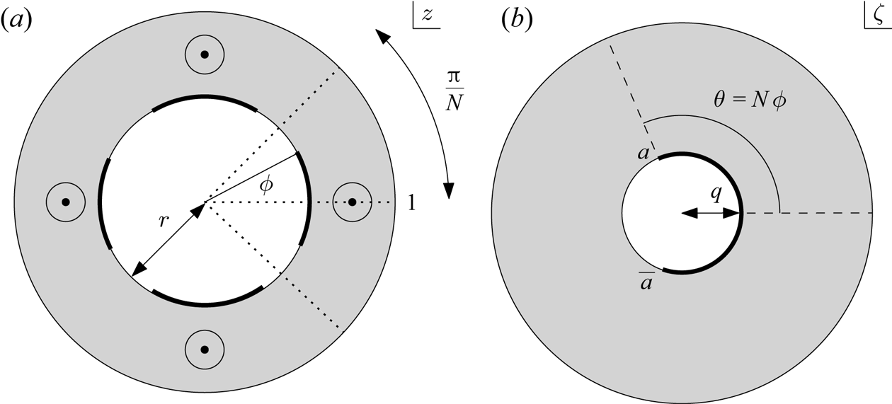
 $h(z)$ in the general solution (2.10). The schematic on the left of figure 3 shows such a configuration for
 $N=4$.
Conformal mapping,  $\zeta =z^N$, between a single
 $2{\rm \pi} /N$ wedge of the
 $N$-fold rotationally symmetric annular pipe
 $r < |z| < 1$ and a full annulus
 $q < |\zeta | < 1$ where
 $q=r^N$ in a parametric
 $\zeta$ plane. The case
 $N=4$ is shown.

On the no-slip outer wall, where  $w(x,y)=0$, we must have
 \begin{equation} \textrm{Re}[h(z)] = 0,\quad \textrm{on}\ |z|=1. \end{equation}
Similarly, on the no-slip portions of  $|z|=r$,
 \begin{equation} \textrm{Re}[h(z)] = \frac{r^2 -1 }{2},\quad \textrm{on}\ |z|=r, (\text{no slip portions}). \end{equation}
Another way to think of this is that the tangential derivative of  $w$ vanishes on these boundary portions
 \begin{equation} \boldsymbol{\nabla} w\boldsymbol{\cdot}{\boldsymbol t} =\begin{cases} \displaystyle{\textrm{Re} \left [ 2\dfrac{\partial w }{\partial z} (-\textrm{i} z) \right]} = 0, & \textrm{on}\ |z|=1,\\ \displaystyle{\textrm{Re} \left [ 2\dfrac{\partial w }{\partial z} \left ( -\dfrac{\textrm{i} z }{r}\right ) \right]}= 0, & \textrm{on}\ |z|=r\, (\text{no slip portions}), \end{cases}\end{equation}
where  ${\boldsymbol t}$ denotes the unit tangent at the surface. The expressions on the right-hand side are just the complex variable form of
 $\boldsymbol {\nabla } w\boldsymbol {\cdot }{\boldsymbol t}$ on the two boundaries. From (2.10),
 \begin{equation} \frac{\partial w }{\partial z} = - \frac{\bar{z} }{4} + \frac{1 }{4} \frac{\textrm{d} h }{\textrm{d} z} \end{equation}
implying that
 \begin{equation} \textrm{Im}\left [z \frac{\textrm{d} h}{\textrm{d} z}\right ] = 0,\quad \textrm{on}\ |z|=1,\ |z|=r\ (\text{the no slip portions}). \end{equation}
On the other hand, on the no-shear portions of  $|z|=r$ the condition is
 \begin{equation} \boldsymbol{\nabla} w\boldsymbol{\cdot}{\boldsymbol n} = 0,\quad \textrm{or}\quad \textrm{Re} \left [ 2\frac{\partial w }{\partial z} \left [ \frac{z }{r}\right ] \right]= \textrm{Re} \left [ z \left [- \frac{\bar{z} }{2} + \frac{1 }{2} \frac{\textrm{d} h }{\textrm{d} z} \right ]\right] = 0, \end{equation}
where  ${\boldsymbol n}$ denotes the unit inward normal at the surface. Hence
 \begin{equation} \textrm{Re} \left [z \frac{\textrm{d} h }{\textrm{d} z} \right ] = r^2,\quad \textrm{on}\ |z|=r\ (\text{no shear portions}). \end{equation}
The function  $z\textrm{d}h/\textrm{d}z$ appears in both forms of the boundary conditions. It is therefore natural to introduce the function
 \begin{equation} g(z) = z \frac{\textrm{d} h}{\textrm{d} z} -r^2 \end{equation}
after which it follows, from (3.7) that
 \begin{equation} \textrm{Re}[g(z)] = 0,\quad \textrm{on}\ |z|=r\ (\text{no shear portions}) \end{equation}
and, from (3.5), that
 \begin{equation} \textrm{Im}[g(z)] = 0,\quad \textrm{on}\ |z|=1,\ |z|=r\ (\text{no slip portions}) . \end{equation}
It is  $g(z)$ that will now be constructed, with
 $h(z)$ then following on integration of (3.8).
One way to interpret (3.9) is that  $g(z)$ has constant argument on the no-shear portions of
 $|z|=r$. Likewise, (3.10) says that
 $g(z)$ has constant argument on the no-slip portions of
 $|z|=r$ and on
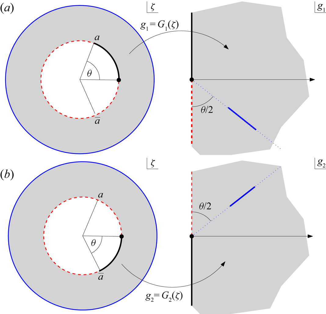
 $|z|=1$. In other words,
 $g(z)$ has piecewise constant argument on all the boundaries of the fluid domain. Those constant values change on passing through the boundary point singularities where a no-slip boundary meets a no-shear boundary portion.
To account for the  $N$-fold rotational symmetry, a new complex variable
 $\zeta$ can be introduced that is related to
 $z$ by
 \begin{equation} \zeta = z^N,\quad z = f(\zeta) = \zeta^{1/N}. \end{equation}
This change of variables can be viewed as a conformal mapping this transplants a typical annular wedge of the fluid domain to the entire annulus  $q < |\zeta |< 1$ in a parametric
 $\zeta$ plane where
 $q=r^N$. Figure 3 shows this correspondence between the
 $z$ and
 $\zeta$ planes.
It is natural to attempt to construct the composed function
 \begin{equation} G(\zeta) \equiv g(z) = g(\,f(\zeta)). \end{equation}
Using ideas presented in Crowdy (Reference Crowdy2020) it can be argued that  $G(\zeta )$ must have the functional form
 \begin{equation} G(\zeta) = -R \left [ \frac{P(\zeta/q,q) P(\zeta/q,q) }{P(\zeta/a,q) P(\zeta/\bar{a},q)} \right ]^{1/2},\quad a= q\,\textrm{e}^{\textrm{i} \theta} = q\,\textrm{e}^{\textrm{i} N \phi},\enspace q=r^N, \end{equation}
where  $R$ is a real constant and the function
 $P(\zeta ,q)$ was introduced in (1.4). The reason for this follows from the observation that, for
 $0 < \theta < {\rm \pi}$, the two functions
 \begin{equation} G_1(\zeta) \equiv -\textrm{i}\,\textrm{e}^{-\textrm{i} \theta/2} \frac{P(\zeta/q,q) }{P(\zeta/a,q) },\quad \textrm{and}\quad G_2(\zeta) \equiv +\textrm{i} \,\textrm{e}^{+\textrm{i} \theta/2} \frac{P(\zeta/q,q) }{P(\zeta/\bar{a},q)}, \end{equation}
when viewed as conformal mappings, each transplants the annulus  $q < |\zeta | < 1$ to a right half-plane with a straight radial slit. These are referred to as Cayley-type maps by Crowdy (Reference Crowdy2020). These mapping properties are readily established on use of the following two functional relations satisfied by the prime function:
 \begin{equation} P(q^2 \zeta, q) = -\zeta^{-1} P(\zeta,q),\quad P(1/\zeta, q) = -\zeta^{-1} P(\zeta,q). \end{equation}
These two relations follow easily from the infinite product definition (1.4). Appendix B gives further details of the construction of  $G(\zeta )$ from the two Cayley-type maps
 $G_1(\zeta )$ and
 $G_2(\zeta )$. The important point is that when
 $|z|=r$ or
 $|z|=1$, so that
 $|\zeta |=q$ or
 $|\zeta |=1$, then each of the functions in (3.14a,b) has constant argument. So too, therefore, does
 $G(\zeta ) = - R \sqrt {G_1(\zeta ) G_2(\zeta )}$ since it is a real multiple of the square root of the product of these two functions. Appendix B gives more details to confirm that
 $G(\zeta )$ is the required function and that is satisfies the boundary conditions (3.9) and (3.10).
It follows that
 \begin{equation} z \frac{\textrm{d} h}{\textrm{d}z} = r^2 +g(z) = r^2 - R \left [ \frac{P(\zeta/q,q) P(\zeta/q,q) }{P(\zeta/a,q) P(\zeta/\bar{a},q)} \right ]^{1/2}, \end{equation}
meaning that we have found  $z \textrm{d}h/\textrm{d}z$ as a function of
 $\zeta$. If we let
 \begin{equation} H(\zeta) \equiv h(z) = h(\,f(\zeta)) \end{equation}
then on use of the two results,
 \begin{equation} z \frac{\textrm{d} h }{\textrm{d} z} = {z} \frac{{\textrm{d} H / \textrm{d} \zeta} }{\textrm{d} f / \textrm{d}\zeta},\quad \frac{z }{\textrm{d} f / \textrm{d}\zeta} = N \zeta, \end{equation}
the first following from the chain rule, the second from (3.11), it follows that
 \begin{equation} H(\zeta) = \frac{1 }{N} \int^\zeta_{-1} \left \lbrace r^2 - R \left [ \frac{P(\zeta/q',q) P(\zeta'/q,q) }{P(\zeta'/a,q) P(\zeta'/\bar{a},q)} \right ]^{1/2} \right \rbrace \frac{\textrm{d} \zeta' }{\zeta'}. \end{equation}
The scaling factor  $R$ is determined by imposing that
 $w(x,y)=0$ on the no-slip portion of
 $|z|=r$. If this condition is imposed at the single point
 $z=r \,\textrm {e}^{\textrm {i} {\rm \pi}/N}$, corresponding to
 $\zeta =-q= -r^N$, then
 \begin{equation} \frac{1 -r^2 }{4} + \frac{1 }{2} \textrm{Re} \left [ \frac{1 }{N} \int^{-r^N}_{-1} \left \lbrace r^2 - R \left [ \frac{P(\zeta/q,q) P(\zeta/q,q) }{P(\zeta/a,q) P(\zeta/\bar{a},q)} \right ]^{1/2} \right \rbrace \frac{\textrm{d} \zeta }{\zeta} \right ] = 0. \end{equation}
By the built-in properties of  $z \textrm{d}h/\textrm{d}z$ the no-slip condition will then hold everywhere on this no-slip portion of
 $|z|=r$ until either of the no-slip/no-shear transition points is reached. A rearrangement of (3.20) leads to the explicit expression
 \begin{align} R = \frac{(1-r^2)/4 + (1/2) r^2 \log r }{S},\quad S \equiv \frac{1 }{2N} \int^{-q}_{-1} \left [ \frac{P(\zeta/q,q) P(\zeta/q,q) }{P(\zeta/a,q) P(\zeta/\bar{a},q)} \right ]^{1/2} \frac{\textrm{d}\zeta }{\zeta}. \end{align}
The solution (1.2) and (1.3) reported earlier then follows.
The effective slip length can be found by identifying that
 \begin{equation} {\mathcal{A}} = \frac{r^2 }{2} - \frac{R I_{-1} }{2 }, \end{equation}
where  $I_{-1}$ is the coefficient of
 $1/\zeta$ in a Laurent expansion of the integrand appearing in the definition of the constant
 $S$ in (3.21a,b). It can be calculated using
 \begin{equation} I_{-1} = \frac{1 }{2 {\rm \pi}\textrm{i}} \oint_{C} \left [ \frac{P(\zeta/q,q) P(\zeta/q,q) }{P(\zeta/a,q) P(\zeta/\bar{a},q)} \right ]^{1/2} \frac{\textrm{d}\zeta }{\zeta}, \end{equation}
where  $C$ is any closed circle inside the annulus
 $q < |\zeta | < 1$ and enclosing the origin. On substitution of
 ${\mathcal {A}}$ from (3.22) into (2.18),
 \begin{equation} \lambda = r \log r - \frac{2 r S }{I_{-1}}, \end{equation}
where  $S$ can be calculated using (3.21a,b) and
 $I_{-1}$ using (3.23). This leads to formula (1.5) recorded earlier.
Limit  $\phi \to 0$ with
 $r, N$ fixed: In this limit the no-shear portion of the inner wall vanishes leading to pure Poiseuille flow along the pipe. In this limit
 $a \to q$ so that
 \begin{equation} \left [ \frac{P(\zeta/q,q) P(\zeta/q,q) }{P(\zeta/a,q) P(\zeta/\bar{a},q)} \right ]^{1/2} \to 1 \end{equation}
and
 \begin{equation} S \to \frac{\log r }{2},\quad R \to \frac{1-r^2 }{2 \log r} + {r^2}, \quad I_{-1} \to 1. \end{equation}
Therefore
 \begin{equation} w(x,y) \to \frac{1 -z \bar{z} }{4} + \frac{r^2-1 }{4 \log r} \log |z|. \end{equation}
This is the axisymmetric solution satisfying the no-slip condition on both walls. The solution dependence on  $N$ vanishes in this limit. It is also found from (3.24) that
 $\lambda \to 0$ as expected.
Limit  $\phi \to {\rm \pi}/N$ with
 $r, N$ fixed: In the opposite limit
 $\phi \to {\rm \pi}/N$ where the inner wall is entirely no shear then
 $a \to -q$ and
 \begin{equation} S \to \infty,\quad R \to 0 \end{equation}
so that
 \begin{equation} w(z) \to \frac{1 - z \bar{z} }{4} + \frac{r^2 }{2} \log |z| , \end{equation}
which is the axisymmetric solution satisfying the boundary conditions
 \begin{equation} w = 0,\enspace \textrm{on}\ |z|=1,\quad \frac{\partial w }{\partial n} = 0,\enspace \textrm{on}\ |z|=r. \end{equation}
The dependence of the solution on  $N$ vanishes in this limit. Since
 $I_{-1}$ remains bounded in this limit, (3.24) now implies that
 $\lambda \to \infty$ as expected.
4. Superhydrophobic annular pipe with patterned outer wall
Consider now the opposite situation of an SH pipe with an outer boundary  $|z|=1$ having
 $N \ge 1$ rotationally symmetric no-shear slots while the boundary
 $|z|=r$ is a no-slip zone. The mathematical arguments in this case are entirely analogous to those detailed in § 3 so we only summarize the results (we will employ similar notation as before, but the quantities will be different). In this case we can argue that
 \begin{equation} G(\zeta) = -R \left [ \frac{P(\zeta,q) P(\zeta,q) }{P(\zeta/a,q) P(\zeta/\bar{a},q)} \right ]^{1/2},\quad a= \textrm{e}^{\textrm{i} \theta} = \textrm{e}^{\textrm{i} N \phi},\enspace q=r^N, \end{equation}
where  $R$ is a real constant; hence
 $H(\zeta )$ for this case is given by (1.6). Notice that the square root branch points of the function (4.1) are now on
 $|\zeta |=1$. The value of
 $R$ is determined by enforcing the no-slip condition on the inner wall
 \begin{equation} \frac{1 -r^2 }{4} + \frac{1 }{2} \textrm{Re} \left [ \frac{1 }{N} \int^{-r^N}_{-1} \left \lbrace 1 - R \left [ \frac{P(\zeta',q) P(\zeta',q) }{P(\zeta'/a,q) P(\zeta'/\bar{a},q)} \right ]^{1/2} \right \rbrace \frac{\textrm{d} \zeta' }{\zeta'} \right ] = 0, \end{equation}
or, explicitly,
 \begin{equation} R = \frac{(1-r^2)/4 + (1/2) \log r }{S},\quad S \equiv \frac{1 }{2N} \int^{-q}_{-1} \left [ \frac{P(\zeta,q) P(\zeta,q) }{P(\zeta/a,q) P(\zeta/\bar{a},q)} \right ]^{1/2} \frac{\textrm{d} \zeta }{\zeta}. \end{equation}
This completes the solution.
The effective slip length follows from the same arguments presented in § 2. Specifically, we find
 \begin{equation} {\mathcal{A}} = \frac{1 }{2} - \frac{R I_{-1} }{2 }, \end{equation}
where
 \begin{equation} I_{-1} = \frac{1 }{2 {\rm \pi}\textrm{i}} \oint_{C} \left [ \frac{P(\zeta,q) P(\zeta,q) }{P(\zeta/a,q) P(\zeta/\bar{a},q)} \right ]^{1/2} \frac{\textrm{d} \zeta }{\zeta}, \end{equation}
where  $C$ is any closed circle inside the annulus
 $q < |\zeta | < 1$ and enclosing the origin. On substitution of this values of
 ${\mathcal {A}}$ into (2.17) we find the effective slip length
 $\lambda$ for this flow to be
 \begin{equation} \lambda= \log r - \frac{2 S }{I_{-1}}, \end{equation}
where  $S$ can be calculated using (4.3a,b) and
 $I_{-1}$ using (4.5). This leads to the formula (1.7).
5. A new form of Philip's pipe flow solution
The pipe flow solution of Philip (Reference Philip1972) has no inner wall but has no-shear slots on the outer wall and therefore must correspond to a limit of our SH pipe solution (1.2) with outer-wall patterning as  $r \to 0$. In this limit,
 $q = r^N \to 0$ and
 $P(\zeta ,q) \to (1-\zeta )$ so that
 $h(z)$ reduces to the form (1.8). In this case
 $R$ is chosen so that
 $H(\zeta )$ is analytic at
 $\zeta =0$. With this expression substituted into (1.2) we arrive at the new form of Philip's pipe flow solution (1.8) with the slip length given by (1.9).
It is worth mentioning here a well-known subtlety associated with the limit  $r \to 0$ of annular pipe flow where the inner pipe wall vanishes. This subtlety exists even for the case where both walls of the pipe are no-slip surfaces and it is in that context that it is usually discussed in fluid dynamics texts (Escudier Reference Escudier2017); we expect the same to be true if either of the tube walls is patterned with no-shear slots. Thinking of pressure-driven Poiseuille flow in a no-slip tube, since the inner tube wall is a no-slip surface and becomes vanishingly small as
 $r \to 0$ it is reasonable to suspect that the limiting boundary value problem, as
 $r \to 0$, is one where the outer wall
 $|z|=1$ is a no-slip surface with the centre of the pipe
 $z=0$ being a stagnation point. However, as can be seen by analysis of the axisymmetric Poiseuille flow solution, what happens is that the radial distance of the circle of maximum axial velocity in the tube also tends to zero as
 $r \to 0$ meaning that the centre of the tube becomes not a stagnation point but the point of maximal velocity. That is, the problem reduces to the standard one of pressure-driven axial flow in a single-walled tube. Physically what happens is that the shear stress associated with the vanishingly small inner wall of the tube as
 $r \to 0$ affects an increasingly small volume of the fluid implying that its influence on the flow completely vanishes in the limit
 $r \to 0$.
6. A new form of Philip's channel flow solution
A simple adaptation of this mathematical approach can be used to derive a new form of Philip's channel flow solution. We emulate Philip's notation and consider flow in a channel of height  ${\hat H}$ with period width
 $2 \hat B$ where
 ${\hat B} > 1$ with a periodic array of no-shear slots occupying the interval
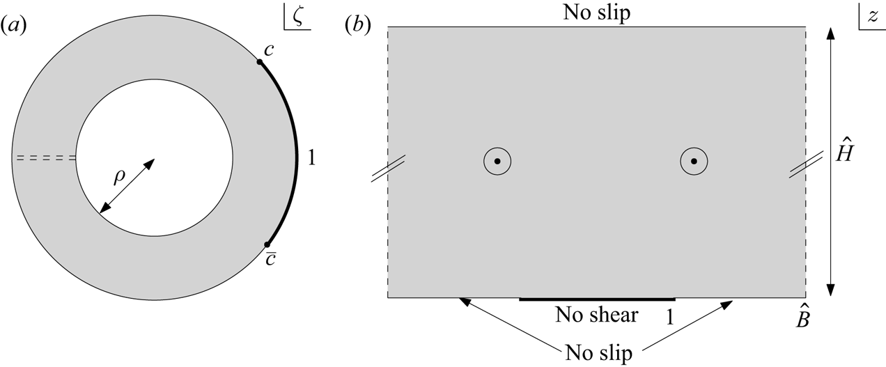
 $(-1,1)$ in the principal period window on the lower wall; see figure 4. Philip (Reference Philip1972) used the same symbols without the hats which have been added here to avoid confusion with the function
 $H(\zeta )$. Let
 \begin{equation} w(x,y)= - \frac{y^2 }{2} + \frac{{\hat H} }{2} \textrm{Re}[ h(z)],\quad z=x+\textrm{i} y. \end{equation}
We now associate  $z$ with a complex variable
 $\zeta$ taking values in an annulus
 $\rho <|\zeta | < 1$ via
 \begin{equation} \zeta=\textrm{e}^{\textrm{i} {\rm \pi}z/\hat B},\quad z = - \frac{\textrm{i} \hat B }{\rm \pi} \log \zeta,\quad \rho = \textrm{e}^{-{\rm \pi} \hat H/\hat B}. \end{equation}
Figure 4 illustrates this change of variables as a conformal mapping: it transplants the annulus  $\rho <|\zeta | < 1$ to the principal period window of Philip's channel flow with the circle
 $|\zeta |=\rho$ corresponding to the upper channel wall at
 $y=\hat H$. The point
 $\zeta =c$ on the unit circle is the preimage of the boundary point where the no-slip boundary meets the no-shear boundary. It can then be argued – using identical reasoning to § 3 – that if we define
 $H(\zeta ) \equiv h(z)$ as before then
 $w(x,y)$ has the form (6.1) now with
 $H(\zeta )$ given by (1.11) for some real constant
 ${\mathcal {R}}$ determined by enforcing that the no-slip condition holds on
 $|\zeta |=\rho$. From (6.1) this means that we need
 \begin{equation} \textrm{Re}[H(-\rho)] = \hat H, \end{equation}
or, explicitly,
 \begin{equation} {\mathcal{R}}= \frac{\hat H }{{\mathcal{S}}},\quad {\mathcal{S}} \equiv \int_{-1}^{-\rho} \left [ \frac{P(\zeta,\rho) P(\zeta,\rho) }{P(\zeta/c,\rho) P(\zeta/\bar{c},\rho)} \right ]^{1/2} \frac{\textrm{d} \zeta }{\zeta}. \end{equation}
Formulas (1.10)–(1.11) give a new form of Philip's channel flow solution.
Philip's channel flow solution (Philip Reference Philip1972): a periodic array of no-shear slots decorates the lower wall of a channel. The upper wall is a no-slip surface. A typical period window is shown in (b). Consideration of the parametric annulus in a complex  $\zeta$ plane in (a) leads to a new form of Philip's solution given in § 6. The point
 $\zeta =c$ corresponds to the edge of the no-shear slot at
 $z=1$.

As discussed earlier, we believe (1.10)–(1.11) is a simpler form of the channel flow solution for practical use than the expression given by Philip (Reference Philip1972) in terms of Jacobi cn functions. Appendix D gives more details on the mathematical connections between these two different representations of the same solution.
To compute the effective slip length we follow a modified strategy akin to that set out in § 2. In the unidirectional flow
 \begin{equation} w(x,y) = - \frac{y^2}{2} + {A} y + {B} \end{equation}
with the Navier-slip condition (2.3a,b) imposed on the lower channel boundary the following relations between  $\lambda$,
 $A$ and
 $B$ can be deduced:
 \begin{equation} \lambda = \frac{{B} }{{A}},\quad {B} = \frac{\hat H^2 }{2} - {A} \hat H. \end{equation}
By similar arguments to those given in § 2 it follows that the effective slip length for the mixed boundary value problem, call it  $\lambda _P^{({channel})}$, is given by
 \begin{equation} \lambda_P^{({channel})} = \frac{{\mathcal{B}} }{{\mathcal{A}}} = \frac{\hat H^2}{2 {\mathcal{A}}} - \hat H, \end{equation}
where the constants  ${\mathcal {A}}$ and
 ${\mathcal {B}}$ are found from the following representation
 \begin{align} w(x,y)= - \frac{y^2}{2} + {\mathcal{A}} y + {\mathcal{B}} + \frac{\hat H}{2}\textrm{Re} \left[\sum_{n \ge 1} \left [{h_n \exp({\textrm{i} {\rm \pi}n z/\hat B})} + {h_{-n} \rho^n \exp({-\textrm{i} {\rm \pi}n z/\hat B})}\right ]\right]\end{align}
of the channel flow solution. As in § 2, this works because of the combination of facts that none of the terms in the infinite sum contribute to the volume flux while all their contributions to  $w(x,y)$ vanish on the upper channel wall by virtue of a condition between
 $h_{-n}$ and
 $h_n$ akin to that in (2.13). Only
 ${\mathcal {A}}$ is therefore needed to find
 $\lambda _P^{({channel})}$ and it is straightforward to identify
 \begin{equation} {\mathcal{A}} = - \frac{{\rm \pi} }{2} \frac{\hat H }{\hat B} {\mathcal{R}} {\mathcal{I}}_{-1},\end{equation}
with
 \begin{equation} {\mathcal{I}}_{-1} = \frac{1 }{2 {\rm \pi}\textrm{i}} \oint_{C} \left [ \frac{P(\zeta,\rho) P(\zeta,\rho) }{P(\zeta/c,\rho) P(\zeta/\bar{c},\rho)} \right ]^{1/2} \frac{\textrm{d} \zeta }{\zeta},\end{equation}
where  $C$ is any closed circle inside the annulus
 $\rho < |\zeta | < 1$ and enclosing the origin. This leads, on substitution of (6.9) into (6.7) and use of (6.4a,b), to
 \begin{equation} \lambda_P^{({channel})} = - \hat H - \frac{\hat B }{\rm \pi} \frac{{\mathcal{S}} }{{\mathcal{I}}_{-1}},\end{equation}
and hence to formula (1.12) recorded earlier.
7. Characterization of the solutions
The characteristics of the new solutions will now be explored, focussing first on those with no-shear patterning on the inner wall as presented in § 3. The expression (1.3) for the function  $H(\zeta )$ involves an integral whose integrand is analytic at all points inside the annulus
 $q < |\zeta | < 1$, but it has integrable square root singularities at
 $a$ and
 $\bar {a}$ on the boundary circle
 $|\zeta |=q$. To compute these integrals one can apply Gauss–Jacobi quadrature, or alternatively use a singularity subtraction strategy since the form of the inverse square root singularity is known explicitly. That singularity can be subtracted off and integrated explicitly with the remaining non-singular integral computed using standard techniques.
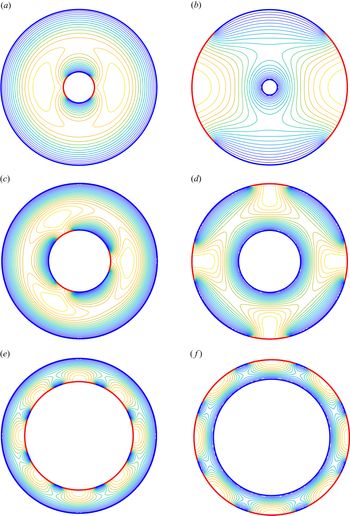
The left column of figure 5 shows contour plots of the axial velocity for several annular SH pipes with no-shear patterning on the inner wall. Cases with  $N=2,3$ and
 $8$ no-shear slots are shown for different values of
 $r$ and
 $\theta$. The right column of figure 5 shows similar contours when the patterning is on the outer wall. The formation of
 $N$-fold rotationally symmetric velocity maxima in the middle of the pipe are clear in all cases.
Constant axial velocity contours for SH pipes with both inner and outer no-shear patterning: (a)  $N=2$,
 $r=0.2$,
 $\theta ={\rm \pi} /2$ (inner); (b)
 $N=2, r=0.1, \theta ={\rm \pi} /2$ (outer); (c)
 $N=3, r=0.4, \theta ={\rm \pi} /3$ (inner); (d)
 $N=4, r=0.4, \theta ={\rm \pi} /3$ (outer); (e)
 $N=8, r=0.7, \theta =4 {\rm \pi}/5$ (inner); (f)
 $N=8, r=0.75, \theta =4 {\rm \pi}/5$ (outer).

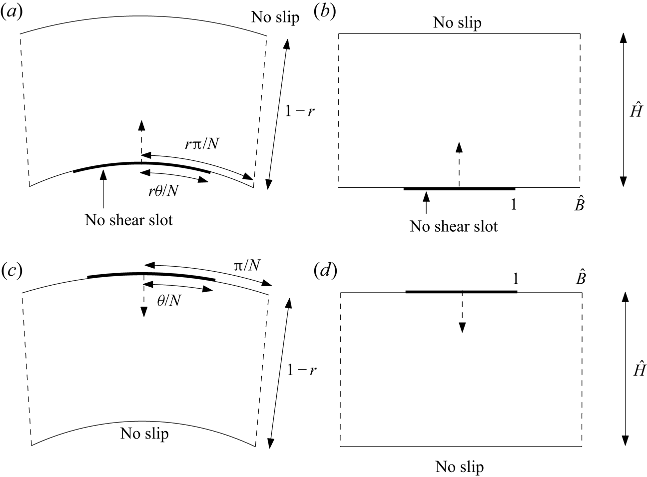
When studying the associated effective slip lengths it is useful to consider some connections to Philip's channel flow solution studied in § 6 by examining various limits as the number of no-shear slots  $N \to \infty$ and/or
 $r \to 1$. Figure 6 indicates why, for any fixed value of
 $\theta = {\rm \pi}/\hat B$, in the double limit as
 $N \to \infty$ and
 $r \to 1$ with
 $N(1-r)$ fixed equal to
 ${\rm \pi} \hat H/\hat B$, the problem in each
 $2{\rm \pi} /N$ sector of the curved annular pipe with a superhydrophobic inner wall tends to the problem in a period window of Philip's periodic channel problem as the radius of curvature effect becomes less significant. To move from the left to the right schematic at the top of figure 6 we must rescale all (non-dimensionalized) lengths by a factor
 $r \theta /N$. To compare with Philip's solution we therefore make the parameter identifications
 \begin{equation} \hat B= \frac{{\rm \pi} }{\theta},\quad \hat H = \frac{(1-r) N }{r\theta}.\end{equation}
Once the effective slip length  $\lambda _P^{({channel})}$ for Philip's channel solution with these parameters has been found, an approximation
 $\lambda _{approx}^{(channel)}$ to the effective slip length for the annular SH pipe problem is
 \begin{equation} \lambda_{approx}^{(channel)} = \frac{r \theta }{N} \lambda_P^{({channel})}.\end{equation}
For a fixed  $\theta = {\rm \pi}/\hat B$ as
 $N \to \infty$ and
 $r \to 1$ with
 $N(1-r)$ fixed equal to
 ${\rm \pi} \hat H/\hat B$, the flow in a typical
 $2{\rm \pi} /N$ annular wedge of the SH pipe ((a,c), where patterning can be on either wall) tends to that in a single period window of Philip's channel flow solution with the parameters shown in (b,d).

Similarly, as shown in the lower schematic in figure 6, for the annular SH pipe with slots on the outer wall the parameter identifications are
 \begin{equation} \hat B= \frac{\rm \pi}{\theta},\quad \hat H = \frac{(1-r) N}{\theta}, \end{equation}
with the approximation  $\lambda _{approx}^{(channel)}$ to the slip length for the annular SH pipe problem given by
 \begin{equation} \lambda_{approx}^{(channel)}= \frac{\theta}{N} \lambda_P^{({channel})}. \end{equation}
In particular, with the identifications (7.3a,b) we have
 \begin{equation} r = 1- \frac{{\rm \pi} \hat H}{N \hat B}, \end{equation}
implying that, in the limit  $N \to \infty$ with
 $\hat H/\hat B$ fixed,
 \begin{equation} q = r^N = \left (1- \frac{{\rm \pi} \hat H }{N \hat B }\right )^N \xrightarrow{N \to \infty} \,\textrm{e}^{-{\rm \pi} \hat H/\hat B} = \rho, \end{equation}
where the last equality follows from (6.2a–c).
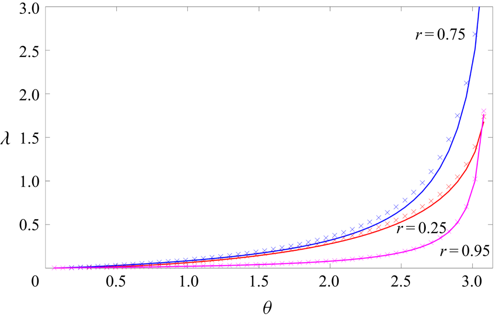
Figure 7 shows the effective slip length  $\lambda$ as a function of
 $\theta$ for fixed
 $N=1$ and three different values of the inner pipe radius
 $r=0.25, 0.75$ and
 $0.95$. The slip length increases with
 $\theta$ as expected given that more of the inner surface is free of shear as
 $\theta$ increases. Indeed,
 $\lambda \to \infty$ as
 $\theta \to {\rm \pi}$ for all values of
 $r$. Also shown in this graph are the approximations given by Philip's channel flow solution which are surprisingly close to the actual slip lengths given that the flow geometries are so different. These approximations tend to slightly overestimate the slip length. The approximation improves with increasing
 $r$ and this feature is explained mathematically in appendix E.
Effective slip length  $\lambda$ for an annular SH pipe with a single
 $N=1$ no-shear slot on the inner wall for
 $r=0.25, 0.75$ and
 $0.95$. Crosses show values from Philip's periodic channel solution
 $\lambda _{approx}^{(channel)}$ as given by (7.1a,b)–(7.2) as a function of
 $\theta$ for the same
 $r$ and
 $N$.

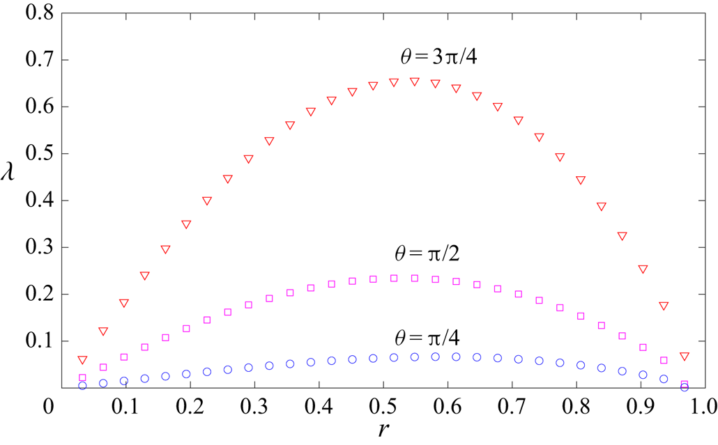
An interesting feature of figure 7 is that the effective slip length  $\lambda$ for a given
 $\theta$ is not monotonic in
 $r$. Figure 8 shows
 $\lambda$ as a function of
 $r$, again for
 $N=1$, and for
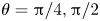 $\theta ={\rm \pi} /4, {\rm \pi}/2$ and
 $3{\rm \pi} /4$. A maximum value of the slip length occurs for a critical value of
 $r$ between
 $0.5$ and
 $0.6$ with these critical values depending only weakly on
 $\theta$. This behaviour can be understood as follows. As
 $r$ increases from zero the effective slip length increases because the no-shear surface area increases with
 $r$. However, when
 $r$ gets sufficiently large that the no-shear interfaces are getting closer to the no-slip outer wall at
 $|z|=1$ a deterioration of the effective slip should occur. Consequently, it is reasonable to expect there to exist a critical
 $r$-value at which
 $\lambda$ is maximized. These critical values of
 $r$ are readily calculated from the explicit formulas and are expected to be useful in optimizing the design of annular SH pipes for maximal friction reduction.
Evidence of a critical value of  $r$ where friction reduction is maximized for an annular SH pipe with no-shear slots on the inner wall. The effective slip length
 $\lambda$ is shown as a function of
 $r$ for
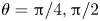 $\theta ={\rm \pi} /4, {\rm \pi}/2$ and
 $3{\rm \pi} /4$ and
 $N=1$.

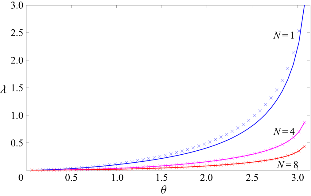
Figure 9 shows the effective slip length  $\lambda$ as a function of
 $\theta$ for fixed
 $r=0.5$ – where we expect the slip to be close to maximal – and for
 $N=1,4$ and
 $8$. Also shown is the approximation given by Philip's channel flow solution
 $\lambda _{approx}^{(channel)}$, as given by (7.1a,b)–(7.2); it is very good across the range of
 $\theta$ values and improves with increasing
 $N$. The effective slip length decreases with
 $N$ – an interesting fact given that, at any fixed
 $\theta$ and
 $r$, the total amount of surface area coverage of the inner boundary by no-shear zones is identical for each value of
 $N$. Recall that
 $\theta /{\rm \pi}$ is the no-shear area fraction which is fixed. The very presence of a boundary point singularity, where the boundary condition changes type, is therefore seen to be deleterious to the friction reducing properties of the pipe. This is another useful fact to be considered in the design of annular SH pipes. A similar observation was made by Yariv & Siegel (Reference Yariv and Siegel2019) in their studies of the torque on a rotating superhydrophobic cylinder.
Effective slip length  $\lambda$ for an annular SH pipe with no-shear slots on the inner wall with
 $r=0.5$ and
 $N=1,4$ and
 $8$. Crosses show values from Philip's periodic channel solution
 $\lambda _{approx}^{(channel)}$ for the same
 $r$ and
 $N$ as calculated using (7.1a,b) and (7.2). More boundary point singularities for the same no-shear fraction means reduced slip.

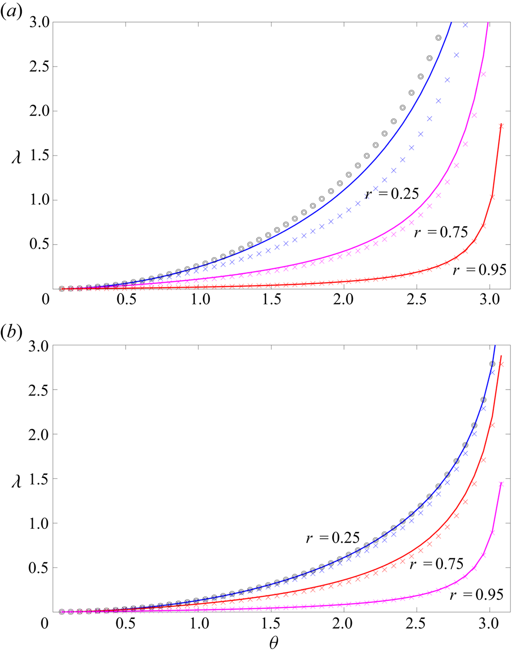
Figure 10 shows the effective slip length  $\lambda$ as a function of
 $\theta$ for
 $r=0.25, 0.75$ and
 $0.95$ with one (
 $N=1$) and two (
 $N=2$) slots on the outer wall as studied in § 4. Superposed on this graph are the corresponding values
 $\lambda _P^{(\,{pipe})}$ for Philip's pipe flow solution calculated using formula (1.9) and Philip's channel flow slip length
 $\lambda _{approx}^{(channel)}$ as calculated using (7.3a,b) and (7.4). For small
 $r$, Philip's
 $\lambda _P^{(\,pipe)}$ is a reasonable approximation to the exact value of
 $\lambda$ for all values of
 $\theta$; the approximation gets worse as
 $r$ increases as expected because the frictional effect of the inner no-slip wall becomes more important as it gets larger, and closer to the outer wall. On the other hand, Philip's
 $\lambda _{approx}^{(channel)}$ becomes a more accurate approximation to
 $\lambda$, across the range of
 $\theta$ values, as
 $r$ increases. Appendix E gives a mathematical explanation of this observation. A useful fact indicated by these graphs is that the true slip length for the annular SH pipes is bounded above by the approximation from Philip's
 $\lambda _P^{(\,{pipe})}$ and from below by Philip's
 $\lambda _{approx}^{(channel)}$.
Effective slip length  $\lambda$ for an annular SH pipe with one (
 $N=1$, upper graph) and two (
 $N=2$, lower graph) no-shear slots on the outer wall for
 $r=0.25, 0.75$ and
 $0.95$. Crosses show corresponding values from Philip's periodic channel solution
 $\lambda _{approx}^{(channel)}$ as given by (7.3a,b)–(7.4); circles show the slip length
 $\lambda _P^{(\,{pipe})}$ from (1.9) for Philip's pipe flow solution.

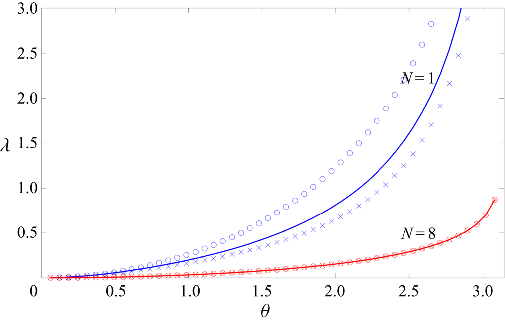
Figure 11 shows the effective slip length for an annular SH pipe with no-shear slots on the outer wall for  $r=0.5$ and
 $N=1,8$ no-shear slots on the outer wall. Approximations provided both by Philip's pipe flow value
 $\lambda _P^{(\,{pipe})}$ and his channel flow value
 $\lambda _{approx}^{(channel)}$ are also shown. There are therefore 3 graphs for each value of
 $N$. For
 $N=8$ the three curves are almost indistinguishable and this is found to be true for higher values of
 $N$. The evidence is that, in the limit
 $N \to \infty$, the value of
 $\lambda _P^{(\,{pipe})}$ from Philip's pipe flow solution gives almost the same approximation to the effective slip length as that obtained by
 $\lambda _{approx}^{(channel)}$ based on Philip's channel flow solution. The mathematical reason for this is given in appendix E.
Effective slip length  $\lambda$ for an annular SH pipe with
 $r=0.5$ and
 $N=1, 8$ no-shear slots on the outer wall. Crosses show values from Philip's periodic channel solution
 $\lambda _{approx}^{(channel)}$ as calculated using (7.3a,b) and (7.4); circles show the slip length
 $\lambda _P^{(\,{pipe})}$ from (1.9) for Philip's pipe flow solution. For
 $N=8$ all three values are indistinguishable.

8. Discussion
This paper has derived analytical solutions for longitudinal flow along concentric annular pipes with no-shear patterning on either the inner or outer wall. The solutions form a 3-parameter family dependent on the number of no-shear slots  $N$, the aspect ratio
 $r$ of the annular pipe, and the no-shear fraction parameter
 $\theta$. Formulas for the effective slip lengths associated with these flows have been established. The results add to a list of analytical solutions for mixed boundary value problems of this kind given by Philip (Reference Philip1972) and the new solutions here are extensions of his.
The author has identified a route to finding solutions for annular pipes with no shear patterning on both walls; those results will be presented elsewhere since they require some additional considerations. Marshall (Reference Marshall2017) has extended Philip's channel solution to the case of a symmetric channel with periodic no shear grooves on both lower and upper walls. Our forthcoming results will extend Marshall's results to the case of annular SH pipes.
Another generalization is to other arrangements of no-shear stripes that are not necessarily  $N$-fold rotationally symmetric. This is possible too, and is a straightforward extension of the present work. To do so involves constructing a generalized function
 $G(\zeta )$ as a square root of a product of more than two Cayley-type maps. This introduces as many square root branch points as needed to supply the boundary point singularities at the edges of the chosen distribution of no-shear slots. At the same time, use of these Cayley-type maps ensures that the resulting function satisfies the required boundary conditions.
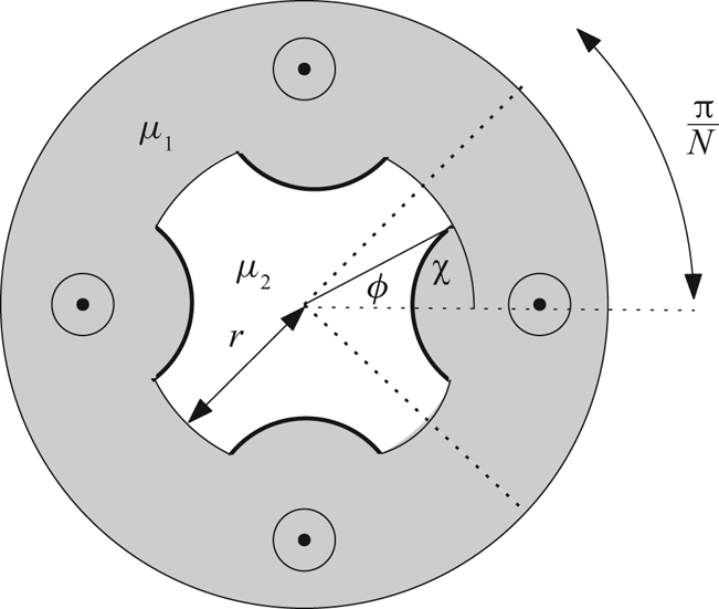
Being non-trivial, and fully capturing the boundary point shear stress singularities between no-slip/no-shear regions, the solutions here will be important in benchmarking numerical codes designed to incorporate more general flow scenarios and capturing more physical effects. Many possible extensions can be envisaged of which figure 12 gives a flavour.
Possible generalizations of the superhydrophobic annular pipe problem: meniscus curvature effects and the addition of a subphase fluid of different viscosity inside the enclosed pipe.

First, the angle between the no-slip surface and the protruding meniscus, defined as angle  $\chi$ in figure 12, need not equal zero as assumed here. Indeed, an overpressure in the working fluid will likely cause deflection of the interface into the central pipe region as shown in figure 12. For channel flows the slip length corrections associated with small-angled meniscus deflection for longitudinal channel flow was studied by Sbragaglia & Prosperetti (Reference Sbragaglia and Prosperetti2007) (see also Crowdy Reference Crowdy2017c) with the generalization of that analysis to transverse flows given by Crowdy (Reference Crowdy2017d). Other authors (Teo & Khoo Reference Teo and Khoo2009) have carried out numerical studies when the deflection is not small. For the longitudinal problem additional theoretical contributions, where the problem is approached as a successively higher-order expansion in the no-shear area fraction but with no constraints on the protrusion angle, have been made by Crowdy (Reference Crowdy2011b, Reference Crowdy2016) with asymptotic analysis of the densely packed case contributed by Schnitzer (Reference Schnitzer2016). Crowdy (Reference Crowdy2017c) has also shown that certain integral relations, combined with Philip's channel flow solutions, can be used to reproduce the slip length correction found (Sbragaglia & Prosperetti Reference Sbragaglia and Prosperetti2007) as a simple integral without any need to solve any new mixed boundary value problems as done by Sbragaglia & Prosperetti (Reference Sbragaglia and Prosperetti2007). A study of analogous effects of non-zero meniscus protrusion angles for the annular SH pipe flows found here is of interest.
Second, the functionality of the core of the annular SH pipes is of interest and there are many practical questions as to how to set up a workable device. In figure 12 we indicate one possibility where the entire core is made up of a second fluid of different viscosity  $\mu _2$. However, it could also consist of the solid rod-like core with a set of surface ‘grooves’ containing a second fluid that the menisci can span. To be close to the shear-free scenario treated here, we would expect
 $\mu _2 \ll \mu _1$ where
 $\mu _1$ is the viscosity of the working fluid in the annular region, but the opposite situation might also be envisaged where the core fluid is more viscous than the working fluid. The no-shear assumption corresponds to setting
 $\mu _2=0$ but this is an idealization. For the channel flow scenario various models of the effect on slip of this second fluid have been offered by Schönecker & Hardt (Reference Schönecker and Hardt2013), Schönecker, Baier & Hardt (Reference Schönecker, Baier and Hardt2014) and Nizkaya, Asmolov & Vinogradova (Reference Nizkaya, Asmolov and Vinogradova2014). A systematic perturbation analysis for the two cases
 $\mu _2 \ll \mu _1$ and
 $\mu _2 \gg \mu _1$ has been carried out by Crowdy (Reference Crowdy2017c) where, again, integral identities play a key role in the analysis. Extension of all this work to annular pipes remains to be made.
Heat transfer applications are also of interest. Kirk, Hodes & Papageorgiou (Reference Kirk, Hodes and Papageorgiou2017) have used the channel flow solution of Philip (Reference Philip1972) as the starting point for a theoretical study of the heat transfer properties associated with such surfaces and its quantification via the Nusselt number. There is an interesting interplay between the enhancement of hydrodynamic slip caused by the introduction of no-shear slots and the compromising effect they have on heat transfer (for example, in cooling the working fluid) compared to a solid no-slip surface. The new solutions found here might form the basis of a similar study of the pipe flow set-up which will help understand the kind of heat transfer optimization challenges considered by Lv & Zhang (Reference Lv and Zhang2016). Another avenue of extension is to a study of thermocapillary effects (Yariv & Crowdy Reference Yariv and Crowdy2019) in annular SH pipes.
As mentioned above, new theoretical results can often be obtained by combining integral identities, such as Green's second identity or the Lorentz reciprocal theorem for Stokes flow, with analytical solutions where the slip length is already known. The results of this paper add to the store of analytical solutions and, as such, open the door to their use in integral identities to find how the slip lengths found here are altered, for example, by non-zero meniscus curvature (Crowdy Reference Crowdy2017c,Reference Crowdyd; Marshall Reference Marshall2017) or by introducing a shear-thinning fluid, a scenario already studied for unbounded shear flows over flat surfaces (Crowdy Reference Crowdy2017a). Using reciprocal theorem identities the associated slip length modifications – usually the quantities of most physical interest – can be found as explicit integrals involving the known analytical solutions and, significantly, without the need to solve the modified flow problem.
Acknowledgements
This work was initiated during the ‘Complex analysis: techniques, applications and computations’ programme at the Newton Institute in Cambridge (Sep-Dec 2019). Support from EPSRC grant EP/R014604/1 is gratefully acknowledged.
Declaration of interests
The author reports no conflict of interest.
Appendix A. Calculation of volume flux contributions
Consider the contribution to the volume flux
 \begin{equation} \int \int_{{r <|z| <1}} w(x,y)\,\textrm{d}\kern0.7pt x\,\textrm{d} y \end{equation}
of a typical term
 \begin{equation} \int \int_{{r <|z| <1}} \textrm{Re} \left [ {h_n z^n} + \frac{h_{-n} r^n }{z^n} \right ] \textrm{d}\kern0.7pt x\,\textrm{d} y,\quad n \ge 1. \end{equation}
This contribution is
 \begin{equation} \textrm{Re} \left [ \int \int_{{r <|z| <1}} \left [{h_n z^n} + \frac{h_{-n} r^n }{z^n} \right ]\textrm{d}\kern0.7pt x\,\textrm{d} y \right ],\quad n \ge 1. \end{equation}
By the complex form of Stokes theorem, and the single-valued nature of the integrand in the annulus, the integral in (A 3) in
 \begin{align} \int \int_{r <|z| <1}\left [{h_n z^n} + \frac{h_{-n} r^n }{z^n} \right ] \textrm{d}\kern0.7pt x\,\textrm{d} y &= \frac{1 }{2 \textrm{i}} \oint_{|z|=1} \left [{h_n z^n} + \frac{h_{-n} r^n }{z^n} \right ] \bar{z} \,\textrm{d} z \nonumber\\ &\quad -\frac{1 }{2 \textrm{i}} \oint_{|z|=r} \left [{h_n z^n} + \frac{h_{-n} r^n }{z^n} \right ] \bar{z}\,\textrm{d} z,\quad n \ge 1. \end{align}
Since  $\bar {z}=1/z$ on
 $|z|=1$ and
 $\bar {z}=r^2/z$ on
 $|z|=r$ then
 \begin{align} \int \int_{{r <|z| <1}}\left [{h_n z^n} + \frac{h_{-n} r^n }{z^n} \right ]\textrm{d}\kern0.7pt x\,\textrm{d} y &= \frac{1 }{2 \textrm{i}} \oint_{|z|=1} \left [{h_n z^n} + \frac{h_{-n} r^n }{z^n} \right]\frac{\textrm{d} z}{z} \nonumber\\ &\quad -\frac{1}{2 \textrm{i}} \oint_{|z|=r} \left [{h_n z^n} + \frac{h_{-n} r^n }{z^n} \right ] \frac{r^2 \,\textrm{d} z}{z} = 0,\quad n \ge 1. \end{align}
Hence, there are no contributions to the volume flux from these terms.
Appendix B. Construction of  $G(\zeta )$ from $G_1(\zeta )$ and $G_2(\zeta )$


This appendix sketches out why  $G(\zeta )$ is the required solution by considering the two Cayley-type maps
 $G_1(\zeta )$ and
 $G_2(\zeta )$ in more detail. More information on the properties of Cayley-type maps can be found in Crowdy (Reference Crowdy2020). Consider the conformal mapping
 \begin{equation} g_1 = G_1(\zeta) = -\textrm{i} \,\textrm{e}^{-\textrm{i} \theta/2} \frac{P(\zeta/q,q) }{P(\zeta/a,q)},\quad a =q \,\textrm{e}^{\textrm{i} \theta},\enspace 0 < \theta < {\rm \pi}. \end{equation}
We will show that the circle  $|\zeta |=1$ maps to a slit in the right half-
 $g_1$ plane; see figure 13. On
 $|\zeta |=1$ we have
 $\zeta = 1/\bar {\zeta }$ so on this circle we can write
 \begin{equation} G_1(\zeta) = -\textrm{i}\,\textrm{e}^{-\textrm{i} \theta/2} \frac{P(1/(q \bar{\zeta}),q) }{P(1/(a \bar{\zeta}),q)}. \end{equation}
On taking the complex conjugate, it is found that
 \begin{equation} \overline{G_1(\zeta)} = +\textrm{i} \,\textrm{e}^{\textrm{i} \theta/2} \frac{P(1/(q {\zeta}),q) }{P(1/(\bar{a} {\zeta}),q)}. \end{equation}
On use of the second identity in (3.15a,b), this becomes
 \begin{equation} \overline{G_1(\zeta)} = +\textrm{i} \,\textrm{e}^{\textrm{i} \theta/2} \frac{\bar{a} }{q} \frac{P(q {\zeta},q) }{P(\bar{a} {\zeta},q)}. \end{equation}
Since  $\bar {a} = q^2/a$ – recall that
 $a$ is on the inner boundary – this can be rewritten as
 \begin{equation} \overline{G_1(\zeta)} = +\textrm{i} \,\textrm{e}^{\textrm{i} \theta/2} \frac{\bar{a} }{q} \frac{P(q^2 \zeta/q,q) }{P(q^2 {\zeta}/a,q)}. \end{equation}
Now the first identity in (3.15a,b) can be used
 \begin{equation} \overline{G_1(\zeta)} = +\textrm{i} \,\textrm{e}^{\textrm{i} \theta/2} \frac{\bar{a} }{a} \frac{P(\zeta/q,q)}{P({\zeta}/a,q)}= \textrm{e}^{\textrm{i} ({\rm \pi}-\theta)} \left (-\textrm{i} \,\textrm{e}^{-\textrm{i} \theta/2} \frac{P(\zeta/q,q) }{P(\zeta/a,q)} \right ) = \textrm{e}^{\textrm{i} ({\rm \pi}-\theta)} G_1(\zeta).\end{equation}
Since
 \begin{equation} \exp({2\textrm{i}\textrm{arg}[G_1(\zeta)]}) = \frac{G_1(\zeta) }{\overline{G_1(\zeta)}} = \textrm{e}^{-\textrm{i} ({\rm \pi}-\theta)}, \end{equation}
where the second equality follows from (B 6), it is seen that the image of  $|\zeta |=1$ has constant argument, equal to
 $-{\rm \pi} /2 + \theta /2$, in the
 $g_1$ plane and lies on the ray shown in figure 13. The restrictions on
 $\theta$ in (B 1) mean that this ray lies in the fourth quadrant.
The geometrical effect of the Cayley-type maps  $G_1(\zeta )$ and
 $G_2(\zeta )$ used to construct
 $G(\zeta )$. Boundary portions of the same colour and line style are in correspondence under each mapping.

It can be shown using similar manipulations that the circle  $|\zeta |=q$ is transplanted to the imaginary axis in the complex
 $g_1$-plane with the arc of this circle between
 $q$ and
 $a$ being transplanted to the positive imaginary axis as shown in figure 13 where boundary portions of the same colour and line style are in correspondence under the mapping. The rest of the circle
 $|\zeta |=q$ is transplanted to the negative imaginary
 $g_1$ axis.
Similar arguments reveal that  $G_2(\zeta )$ has the mapping properties depicted in figure 13 where, again, boundary portions of the same colour and line style correspond under this mapping.
Now consider the function
 \begin{equation} {\mathcal{G}}(\zeta) = G_1(\zeta) G_2(\zeta). \end{equation}
By inspection of figure 13 it is clear that if  $\zeta$ lies on the circle
 $|\zeta |=q$ on the arc joining
 $\bar {a}$ to
 $q$ to
 $a$ – that is, on the no-shear slot in the physical plane – then
 ${\mathcal {G}}(\zeta )$, which is the product of the corresponding values of
 $g_1$ and
 $g_2$, is a negative real number. If
 $\zeta$ lies on any other portion of the boundary – and this is the preimage of the no-slip boundary portions in the physical plane – then
 ${\mathcal {G}}(\zeta )$ is a positive real number. The function
 $G(\zeta )$ introduced in (3.13) is
 \begin{equation} G(\zeta) = - R \sqrt{{\mathcal{G}}(\zeta)}, \end{equation}
where  $R$ is a real constant. Consequently,
 $G(\zeta )$ will be purely imaginary on the no-shear slot (i.e. it will have zero real part) and will be purely real on any no-slip boundary portion (i.e. it will have zero imaginary part). These are precisely the boundary conditions (3.9) and (3.10).
Appendix C. Connection to Philip's pipe flow solution
In the limit  $r \to 0$ the solution (1.2) with
 $h(z)$ defined in (1.6) gives
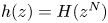 $h(z) = H(z^N)$ where, in this limit,
 \begin{equation} H(\zeta) \to \frac{1}{N} \int^\zeta_{-1} \left \lbrace 1 - {\left (\frac{(1-\zeta')(1-\zeta') }{(1-\zeta'/a) (1-\zeta'/\bar{a})} \right )^{1/2}} \right \rbrace \frac{\textrm{d} \zeta' }{\zeta'},\quad a = \textrm{e}^{\textrm{i} \theta},\end{equation}
which can be written as
 \begin{equation} H(\zeta) = \frac{1 }{N} \int^\zeta_{-1} \left \lbrace 1 - {\left (\frac{\zeta'+1/\zeta' -2 }{\zeta'+1/\zeta'- 2 \cos \theta} \right )^{1/2}} \right \rbrace \frac{\textrm{d} \zeta' }{\zeta'}.\end{equation}
A change of variables  $\zeta =\textrm {e}^{2 \textrm {i} u}$, and use of trigonometric ‘double-angle’ identities, lead to
 \begin{equation} H(\zeta) = \frac{2 \textrm{i} }{N} \int^u_{{\rm \pi}/2} \left[ 1 - \frac{\sin u' }{\sqrt{\cos^2(\theta/2) - \cos^2(u')}} \right ] \textrm{d} u',\quad u = - \frac{\textrm{i} }{2} \log \zeta. \end{equation}
A further change of variables  $\cos (\theta /2) w = \cos u$ yields
 \begin{align} H(\zeta) &= \frac{2 \textrm{i} }{N} \left [ u - \frac{{\rm \pi} }{2} + \int_0^w \frac{\textrm{d} w' }{\sqrt{1-w^{'2}}} \right ] = \frac{2 \textrm{i} }{N} \left [ u - \cos^{-1}(w) \right ] \nonumber\\ &= \frac{2 \textrm{i} }{N} \left [ u - \cos^{-1}\left ( \frac{\cos u }{\cos(\theta/2)} \right ) \right ]. \end{align}
It is inferred from (1.2) that
 \begin{equation} w(x,y) = \frac{1 }{4} (1-|z|^2) + \frac{1 }{N} \textrm{Im} \left [ -u + \cos^{-1}\left ( \frac{\cos u }{\cos(\theta/2)} \right ) \right ], \end{equation}
where
 \begin{equation} u = - \frac{\textrm{i} }{2} \log \zeta = - \frac{\textrm{i} N }{2} \log z. \end{equation}
This is exactly the solution in § 6 of Philip (Reference Philip1972) once the following identifications between parameters are made:
 \begin{equation} \frac{\hat s }{\hat \mu} = 1,\quad \hat q = N,\quad \frac{\hat q \hat b }{\rm \pi} = 1,\quad \frac{\hat a }{\hat b} = \frac{\theta }{\rm \pi},\quad \hat \alpha = \frac{\theta }{2}= \frac{{\rm \pi} \hat a }{2 \hat b},\quad \hat \varTheta = \hat R z = \frac{\hat q }{2 \hat \alpha} z, \end{equation}
where the hatted variables refer to those used, without hats, by Philip (Reference Philip1972).
Appendix D. Connection to Philip's channel flow solution
It is also useful to give a concrete demonstration of how the channel solution derived in § 6 connects with the original solution (Philip Reference Philip1972) who writes it as
 \begin{equation} w(x,y) = - \frac{y^2 }{2} + \frac{y \hat H }{2} + \frac{\hat H W_{10} }{2},\end{equation}
with
 \begin{equation} W_{10} = \textrm{Im} \left [ \frac{\hat H }{K'(k_1)} \textrm{cn}^{-1} \left [ \frac{\textrm{cn}(\hat B^{-1} K(k) z, k) }{\textrm{cn}(\hat B^{-1} K(k), k) } \right ]- z \right ]. \end{equation}
On the other hand, the new form of the same solution found in (1.10) is
 \begin{equation} w(x,y)= - \frac{y^2 }{2} + \frac{{\hat H} }{2}\textrm{Re}[H(\zeta)], \quad \zeta = \textrm{e}^{\textrm{i} {\rm \pi}z/\hat B}, \end{equation}
with  $H(\zeta )$ defined in (1.11). A comparison of (D 1) and (D 3) leads to
 \begin{equation} \textrm{Im} \left [ \frac{\hat H }{K'(k_1)} \textrm{cn}^{-1} \left [ \frac{\textrm{cn}(\hat B^{-1} K(k) z, k) }{\textrm{cn}(\hat B^{-1} K(k), k) }, k_1 \right ] \right ] = \textrm{Re}[H(\zeta)], \end{equation}
from which it emerges that, for the two solutions to be equivalent,
 \begin{equation} \frac{\hat H }{K'(k_1)} \textrm{cn}^{-1} \left [ \frac{\textrm{cn}(\hat B^{-1} K(k) z, k) }{\textrm{cn} (\hat B^{-1} K(k), k) }, k_1 \right ] = \textrm{i} H(\zeta) + C,\end{equation}
where  $C \in \mathbb {R}$ is some real constant. The moduli
 $k$ and
 $k_1$ and the complete elliptical integrals
 $K(k)$ and
 $K'(k_1)$ are all explained in Philip (Reference Philip1972) (we did not add hats to these quantities). It turns out that
 $C=\hat B_1$ where, as we have done with
 $B$ and
 $H$, we have added a hat to a quantity
 $B_1$ that enters Philip's calculation. One way to understand this choice of
 $C$ is to think geometrically.
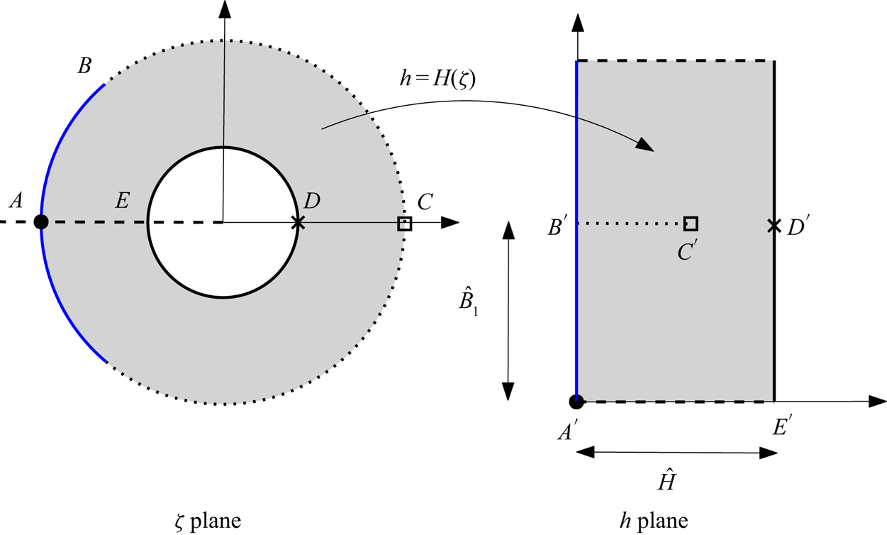
Philip's analysis involves constructing the left-hand side of (D 5) as a conformal mapping from a period window of the flow in the physical plane to a slit rectangle in another complex plane. Analogously, figure 14 shows geometrically how the function  $H(\zeta )$ given in (1.11) acts as a conformal mapping from the annulus
 $\rho < |\zeta | < 1$ to a complex
 $h$ plane:
 $\zeta \mapsto h=H(\zeta )$. The choice (6.4a,b) of the scaling parameter
 ${\mathcal {R}}$ makes sure that the distance between the image of points
 $A'$ and
 $E'$ is
 $\hat H$. Philip (Reference Philip1972) constructs his channel flow solution using (two applications of) the Schwarz–Christoffel formula to transplant the original period window on the complex
 $z$ plane to a ‘slit rectangle’ with side lengths
 $2 \hat B_1$ and
 $\hat H$ very similar to that shown on the right in figure 14, the only difference being the orientation and location of this slit rectangle. By rotating the rectangle on the right in figure 14 by
 $90^{\circ }$ and then shifting it to the right by
 $\hat B_1$ we arrive at Philip's slit rectangle. Equivalently,
 \begin{equation} \textrm{i} H(\zeta) + \hat B_1, \end{equation}
must correspond to the left-hand side of (D 5). In this way we arrive at the identity
 \begin{equation} \frac{\hat H }{K'(k_1)} \textrm{cn}^{-1} \left[\frac{\textrm{cn}(\hat B^{-1} K(k) z, k) }{\textrm{cn}(\hat B^{-1} K(k), k) }, k_1 \right ] - \hat B_1 = \textrm{i} H(\textrm{e}^{\textrm{i} {\rm \pi}z/\hat B}). \end{equation}
This identity, which can be verified numerically, shows explicitly how our construction – which uses only the right-hand side of (D 7) – has replaced the need to consider the Jacobi cnoidal function and its inverse. Interested readers can find other similar identities relating the prime function  $P(\zeta ,q)$ to the classical elliptic functions of Jacobi and Weierstrass in chapter 8 of Crowdy (Reference Crowdy2020).
The function  $H(\zeta )$ from (1.11) interpreted as a conformal mapping from the annulus
 $\rho < |\zeta | < 1$ to a ‘slit rectangle’ in a complex
 $h$-plane. Points labelled by the same letter correspond under the mapping, e.g.
 $A \mapsto A'$.

Appendix E. Analysis of the approximations
The evidence from figures 7, 9, 10 and 11 is that the approximations  $\lambda _{approx}^{(channel)}$ as given with the identifications in (7.1a,b)–(7.2) for patterning on the inner wall, and by (7.3a,b)–(7.4) for patterning on the outer wall, are increasingly accurate in the limit
 $r \to 1$ for any fixed
 $N$ and
 $\theta$. The explicit formulas of this paper can be used to see why this occurs. To explain figure 10, for example, let us suppose that
 $N$ is fixed but that
 $r \to 1$. From the identifications (7.3a,b) and (1.11) note first that
 \begin{equation} c = \textrm{e}^{\textrm{i}{\rm \pi}/\hat B} = \textrm{e}^{\textrm{i}\theta} = a,\end{equation}
where we have also used the definition (4.1) of  $a$ for solutions with outer-wall patterning. As
 $r \to 1$, from the definition (4.1) of
 $q$ we can use a Taylor expansion
 \begin{equation} q = r^N = (1+ (r-1))^N \approx 1 + N (r-1) + \ldots. \end{equation}
On the other hand, use of the identifications (7.3a,b) in (6.2a–c) gives
 \begin{equation} \rho = \textrm{e}^{-{\rm \pi} \hat H / \hat B} = \textrm{e}^{N(r-1)} \approx 1+ N(r-1)+ \cdots, \end{equation}
where have used another Taylor expansion, implying that as  $r \to 1$,
 \begin{equation} q \approx \rho. \end{equation}
Using (E 1) and (E 4) when comparing (4.3a,b) and (6.4a,b) gives
 \begin{equation} S \approx \frac{{\mathcal{S}} }{2N},\end{equation}
and, when comparing (4.5) and (6.10),
 \begin{equation} I_{-1} \approx {\mathcal{I}}_{-1}. \end{equation}
Use of the identifications (7.3a,b) in (7.4) and (6.11) implies that
 \begin{equation} \lambda_{approx}^{(channel)} = \frac{\theta }{N} \lambda_P^{(channel)} = \frac{\theta }{N} \left [ - \hat H - \frac{\hat B }{\rm \pi} \frac{{\mathcal{S}} }{{\mathcal{I}}_{-1}} \right ] = (r-1) - \frac{{\mathcal{S}} }{N {\mathcal{I}}_{-1}}.\end{equation}
But from (4.6) the effective slip length for patterning on the outer wall is
 \begin{equation} \lambda= \log r - \frac{2 S }{I_{-1}} \approx (r-1) - \frac{{\mathcal{S}} }{N {\mathcal{I}}_{-1}}, \end{equation}
where, in the final step, we have used (E 5) and (E 6) and the first term  $\log r \approx r-1$ of the Taylor expansion of
 $\log r$ near
 $r=1$. We have therefore shown, on combining (E 7) and (E 8), that
 \begin{equation} \lambda \approx \lambda_{approx}^{(channel)} \end{equation}
as  $r \to 1$. This is why the approximation given by Philip's channel flow solution gives such good agreement with the effective slip lengths of the new annular SH pipes in this limit.
Similarly, figure 11 reveals that, as  $N \to \infty$ for a fixed
 $r$, not necessarily close to 1, the value of
 $\lambda _P^{({pipe})}$ from Philip's pipe flow solution, gives almost the same approximation to the effective slip length for an SH pipe with patterning on the outer wall as that obtained by the approximation
 $\lambda _{approx}^{(channel)}$ from (7.4) based on Philip's channel flow solution. This feature was pointed out at the end of § 7 and is especially apparent for the
 $N=8$ curve in figure 11. To show why this is the case, note that it has already been observed using the identifications (7.3a,b) that
 \begin{equation} c = \textrm{e}^{\textrm{i}{\rm \pi}/\hat B} = \textrm{e}^{\textrm{i}\theta} =a. \end{equation}
From the scaling (7.3a,b),  $\hat H/\hat B \to \infty$ as
 $N \to \infty$, implying that
 $\rho \to 0$ as is evident from (6.2a–c); in fact,
 $\rho \to 0$ exponentially fast as
 $\hat H/\hat B \to \infty$. It follows from (1.4) that as
 $\rho \to 0$,
 \begin{equation} \left[\frac{P(\zeta,\rho) P(\zeta,\rho) }{P(\zeta/c,\rho) P(\zeta/\bar{c},\rho)}\right ]^{1/2} \frac{1}{\zeta}\approx \left [ \frac{(1-\zeta)^2 }{(1-\zeta/a) (1-\zeta/\bar{a})}\right ]^{1/2} \frac{1 }{\zeta}. \end{equation}
Therefore, in this same limit,
 \begin{equation} {\mathcal{I}}_{-1} \approx 1,\quad {\mathcal{S}} \approx \int^{-\rho}_{-1} \left[\frac{(1-\zeta)^2 }{(1-\zeta/a) (1-\zeta/\bar{a})}\right]^{1/2} \frac{\textrm{d} \zeta }{\zeta}, \end{equation}
where it is important to retain the  $\rho$-dependence in the limit of the integral. Use of this and (7.3a,b) yields
 \begin{equation} \lambda_{approx}^{(channel)}= \frac{\theta }{N} \lambda_P^{(channel)} = \frac{\theta }{N} \left [- \hat H - \frac{\hat B }{\rm \pi} \frac{{\mathcal{S}} }{{\mathcal{I}}_{-1}} \right ] \approx (r-1) - \frac{{\mathcal{S}} }{N}.\end{equation}
From the definition (6.2a–c) of  $\rho$ and (7.3a,b) we can write
 \begin{equation} r-1 = \frac{\log \rho }{N} = \frac{1 }{N} \int_{-1}^{-\rho} \frac{\textrm{d} \zeta }{\zeta}. \end{equation}
On use of this and (E 12) in (E 13) produces
 \begin{equation} \lambda_{approx}^{(channel)} \approx \frac{1 }{N} \int_{-1}^{0} \left [ 1- \left (\frac{(1-\zeta)^2 }{(1-\zeta/a) (1-\zeta/\bar{a})} \right )^{1/2} \right ] \frac{\textrm{d} \zeta }{\zeta},\end{equation}
where, owing to the regularity of the integrand as  $\zeta \to 0$, the contribution to the integral from the interval
 $0$ and
 $\rho$ will be small as
 $\rho \to 0$. Hence, on recognizing
 $\lambda _P^{({pipe})}$ on the right-hand side from (1.9), it follows that as
 $N \to \infty$ with the identifications (7.3a,b),
 \begin{equation} \lambda_{approx}^{(channel)} \approx \lambda_P^{({pipe})}.\end{equation}
In this way it is seen how the new explicit forms of the different solutions facilitate their analysis and comparison in various limits, and without the need to appeal to any special function identities.