2.1 Available energy in ideal MHD

Eliminating the density from the continuity equation (2.1) and the adiabatic law (2.7) gives

(2.11) $$\begin{eqnarray}\frac{\unicode[STIX]{x2202}p^{1/\unicode[STIX]{x1D6FE}}}{\unicode[STIX]{x2202}t}+\unicode[STIX]{x1D735}\boldsymbol{\cdot }\left(p^{1/\unicode[STIX]{x1D6FE}}\boldsymbol{V}\right)=0,\end{eqnarray}$$

which implies that the quantity

(2.12) $$\begin{eqnarray}S=\left\langle p^{1/\unicode[STIX]{x1D6FE}}\right\rangle\end{eqnarray}$$

is conserved, $\text{d}S/\text{d}t=0$ . We thus have two conserved quantities, and may seek the maximum of the magnetic energy

(2.13) $$\begin{eqnarray}M=\left\langle \frac{B^{2}}{2}\right\rangle\end{eqnarray}$$

under the constraint of constant $W$ and $S$ . Since $M<W$ , it is clear that this maximum indeed exists and represents a mathematical upper bound on the magnetic energy at all times $t\geqslant 0$ . It may, however, be inaccessible from the initial conditions, because there is an infinity of other constraints associated with the topology of the magnetic-field lines (Taylor & Newton Reference Taylor and Newton2015), but we ignore this issue as we only seek an upper bound on $M$ that need not be the best possible one.

Thus, we consider the maximum of the functional

(2.14) $$\begin{eqnarray}T[\unicode[STIX]{x1D70C},\boldsymbol{V},\boldsymbol{B},p;\unicode[STIX]{x1D706},\unicode[STIX]{x1D707}]=M-\unicode[STIX]{x1D706}(W-W_{0})-\unicode[STIX]{x1D707}(S-S_{0}),\end{eqnarray}$$

where $\unicode[STIX]{x1D706}$ and $\unicode[STIX]{x1D707}$ are Lagrange multipliers, and initial conditions are denoted by a ‘ $0$ ’ subscript. Since this functional does not involve any derivatives of the fields $(\unicode[STIX]{x1D70C},\boldsymbol{V},\boldsymbol{B},p)$ , these must be constant at the maximum in question; this becomes obvious if one writes down the Euler–Lagrange equations for the minimising fields.Footnote ⁴ Denoting these quantities by the subscript ‘ $1$ ’, we thus have

(2.15) $$\begin{eqnarray}S=\left\langle p_{0}^{1/\unicode[STIX]{x1D6FE}}\right\rangle =p_{1}^{1/\unicode[STIX]{x1D6FE}}\end{eqnarray}$$

and $V_{1}=0$ , so that

(2.16) $$\begin{eqnarray}M_{1}=W-\frac{\left\langle p_{0}^{1/\unicode[STIX]{x1D6FE}}\right\rangle ^{\unicode[STIX]{x1D6FE}}}{\unicode[STIX]{x1D6FE}-1}.\end{eqnarray}$$

The difference between the upper bound $M_{1}$ and the initial value of the magnetic energy, $M_{0}$ , is thus

(2.17) $$\begin{eqnarray}A=M_{1}-M_{0}=\frac{\left\langle p_{0}\right\rangle -\left\langle p_{0}^{1/\unicode[STIX]{x1D6FE}}\right\rangle ^{\unicode[STIX]{x1D6FE}}}{\unicode[STIX]{x1D6FE}-1}+\left\langle \frac{\unicode[STIX]{x1D70C}_{0}V_{0}^{2}}{2}\right\rangle .\end{eqnarray}$$

This quantity is always positive because, for $\unicode[STIX]{x1D6FE}>1$ ,

(2.18) $$\begin{eqnarray}\left\langle p_{0}^{1/\unicode[STIX]{x1D6FE}}\right\rangle \leqslant \left\langle p_{0}\right\rangle ^{1/\unicode[STIX]{x1D6FE}}\end{eqnarray}$$

by Hölder’s inequality.

The expression (2.17) represents an upper bound on the amount of thermal and kinetic energy that is available for conversion into magnetic energy, and will in the following be referred to as the ‘available energy’ for dynamo action. This upper bound is usually inaccessible: not only does it ignore topological constraints on the evolution of the magnetic field, but it is also in general incompatible with the boundary conditions. As we shall see, it can nevertheless be surprisingly restrictive.

If the initial state is such that either the Mach number is of order unity or the pressure $p_{0}$ varies substantially (by order unity) across the domain, then a substantial fraction of the thermal and kinetic energy is available for conversion into magnetic energy, $A/W=O(1)$ . If, however, the initial pressure fluctuations are small,

(2.19) $$\begin{eqnarray}p_{0}(\boldsymbol{r})=P+\unicode[STIX]{x1D6FF}p(\boldsymbol{r}),\end{eqnarray}$$

where $P=\left\langle p_{0}\right\rangle$ and $\unicode[STIX]{x1D6FF}p\ll P$ , then the available energy from these fluctuations is quadratic in their amplitude and is relatively small:

(2.20) $$\begin{eqnarray}A_{\unicode[STIX]{x1D6FF}p}=\frac{\left\langle \unicode[STIX]{x1D6FF}p^{2}\right\rangle }{2\unicode[STIX]{x1D6FE}P}\ll W.\end{eqnarray}$$

If we consider specifically the limit of small Mach numbers (subsonic motions):

(2.21) $$\begin{eqnarray}Ma\equiv \frac{V_{0}}{\sqrt{\unicode[STIX]{x1D6FE}p_{0}/\unicode[STIX]{x1D70C}_{0}}}\ll 1,\end{eqnarray}$$

the dynamics is pressure balanced and, typically, pressure perturbations are $\unicode[STIX]{x1D6FF}p/p_{0}\sim Ma^{2}$ . This means that, to lowest order in $Ma$ , the available energy is just the kinetic energy in the initial state, $K_{0}=\left\langle \unicode[STIX]{x1D70C}_{0}V_{0}^{2}/2\right\rangle$ :

(2.22) $$\begin{eqnarray}\frac{A}{K_{0}}=1+O(Ma).\end{eqnarray}$$

2.2 Finite resistivity and viscosity

Most dynamos considered in the literature involve resistivity, which enables field line diffusion and reconnection to take place. A justified question is, therefore, to what extent the above conclusions remain valid if a finite resistivity is introduced. The induction equation (2.3) then becomes

(2.23) $$\begin{eqnarray}\frac{\unicode[STIX]{x2202}\boldsymbol{B}}{\unicode[STIX]{x2202}t}=\unicode[STIX]{x1D735}\times (\boldsymbol{V}\times \boldsymbol{B})+\unicode[STIX]{x1D702}\unicode[STIX]{x1D6FB}^{2}\boldsymbol{B},\end{eqnarray}$$

and the entropy conservation law (2.7) is replaced by

(2.24) $$\begin{eqnarray}\frac{\text{d}}{\text{d}t}\left(\frac{p}{\unicode[STIX]{x1D70C}^{\unicode[STIX]{x1D6FE}}}\right)=\frac{(\unicode[STIX]{x1D6FE}-1)\unicode[STIX]{x1D702}j^{2}}{\unicode[STIX]{x1D70C}^{\unicode[STIX]{x1D6FE}}}.\end{eqnarray}$$

The energy $W$ is still conserved, but the quantity $S=\left\langle p^{1/\unicode[STIX]{x1D6FE}}\right\rangle$ now increases with time

(2.25) $$\begin{eqnarray}S(t)>S_{0},\end{eqnarray}$$

reflecting positive entropy production. However, regardless of how much $S$ increases, we may still seek the maximum magnetic energy $M_{1}$ at a given $W$ and $S=S_{1}$ and thus find an upper bound on the available energy

(2.26) $$\begin{eqnarray}A=M_{1}-M_{0}=\frac{\left\langle p_{0}\right\rangle -S_{1}^{\unicode[STIX]{x1D6FE}}}{\unicode[STIX]{x1D6FE}-1}+\left\langle \frac{\unicode[STIX]{x1D70C}_{0}V_{0}^{2}}{2}\right\rangle .\end{eqnarray}$$

Since $S_{1}>S_{0}$ , this bound is lower than in the ideal MHD case, and we conclude that less energy is available for conversion to magnetic energy. In other words, the bound (2.17) still holds, but is even tighter than before.

The addition of viscosity to the MHD equations has a similar effect, with viscosity now contributing to entropy production (2.24). Since the total energy (2.10) is conserved and $S(t)$ increases with time, the magnetic energy is again bounded from above by (2.17).

2.3 Available energy in the double-adiabatic model

As we shall now see, the situation is very different in the double-adiabatic model of Chew, Goldberger and Low (Chew et al. Reference Chew, Goldberger and Low1956; Kulsrud Reference Kulsrud, Rosenbluth and Sagdeev1983). Eliminating the density from the continuity equation (2.1) and from the equations of state (2.8) and (2.9) gives

(2.27) $$\begin{eqnarray}\displaystyle & \displaystyle \frac{\unicode[STIX]{x2202}}{\unicode[STIX]{x2202}t}\left(\frac{p_{\bot }}{B}\right)+\unicode[STIX]{x1D735}\boldsymbol{\cdot }\left(\frac{p_{\bot }\boldsymbol{V}}{B}\right)=0, & \displaystyle\end{eqnarray}$$

(2.28) $$\begin{eqnarray}\displaystyle & \displaystyle \frac{\unicode[STIX]{x2202}}{\unicode[STIX]{x2202}t}\left(p_{\Vert }^{1/3}B^{2/3}\right)+\unicode[STIX]{x1D735}\boldsymbol{\cdot }\left(p_{\Vert }^{1/3}B^{2/3}\boldsymbol{V}\right)=0, & \displaystyle\end{eqnarray}$$

implying that the following two quantities are conservedFootnote ⁵

(2.29) $$\begin{eqnarray}\displaystyle & \displaystyle I=\left\langle \frac{p_{\bot }}{B}\right\rangle , & \displaystyle\end{eqnarray}$$

(2.30) $$\begin{eqnarray}\displaystyle & \displaystyle J=\left\langle p_{\Vert }^{1/3}B^{2/3}\right\rangle . & \displaystyle\end{eqnarray}$$

We may thus ask for the maximum of the magnetic energy $M$ under the constraint that $W$ , $I$ and $J$ are fixed. Proceeding as before, we find that all the fields $(p_{\bot },p_{\Vert },B,\ldots )$ are constant and the flow velocity vanishes, so in the state of maximum magnetic energy we have

(2.31) $$\begin{eqnarray}W=IB_{1}+\frac{J^{3}}{2B_{1}^{2}}+\frac{B_{1}^{2}}{2}.\end{eqnarray}$$

This equation is a quartic for $B_{1}$ as a function of the invariants $I$ , $J$ and $W$ , and in terms of the normalised magnetic field $b=B_{1}/\sqrt{W}$ , it becomes

(2.32) $$\begin{eqnarray}b^{4}+\frac{2Ib^{3}}{\sqrt{W}}-2b^{2}+\frac{J^{3}}{W^{2}}=0.\end{eqnarray}$$

The sum of all four roots is equal to $-2I/\sqrt{W}<0$ , while their product equals $J^{3}/W^{2}>0$ . There are, therefore, two positive and two negative roots. The negative ones can obviously be discarded, and the largest positive root is the upper bound that we are seeking. The other positive root is a lower bound on the magnetic energy, for the constancy of $J$ implies that $B$ cannot be made arbitrarily small at constant $W$ , since small $B$ implies large $p_{\Vert }$ . This is different from the ideal MHD case, where the analogous calculation yields no lower bound on $M$ other than $B=0$ .

In the initial state, the ratio of thermal to magnetic energy is equal to

(2.33) $$\begin{eqnarray}\frac{3\unicode[STIX]{x1D6FD}_{0}}{2}=\frac{\left\langle p_{\bot 0}+p_{\Vert 0}/2\right\rangle }{M_{0}}=\frac{W-\unicode[STIX]{x1D70C}_{0}V_{0}^{2}/2}{M_{0}}-1,\end{eqnarray}$$

and in the state of maximum magnetic energy it is

(2.34) $$\begin{eqnarray}\frac{3\unicode[STIX]{x1D6FD}_{1}}{2}=\frac{W}{M_{1}}-1=\frac{2}{b^{2}}-1.\end{eqnarray}$$

The general solution of (2.32) is not particularly edifying, but it does yield interesting information in the limit of high $\unicode[STIX]{x1D6FD}_{0}$ . In this limit,

(2.35) $$\begin{eqnarray}\displaystyle & \displaystyle \frac{I}{\sqrt{W}}\sim \sqrt{\unicode[STIX]{x1D6FD}_{0}}\gg 1, & \displaystyle\end{eqnarray}$$

(2.36) $$\begin{eqnarray}\displaystyle & \displaystyle \frac{J^{3}}{W^{2}}\sim \frac{1}{\unicode[STIX]{x1D6FD}_{0}}\ll 1, & \displaystyle\end{eqnarray}$$

and it is helpful to write $x=b\sqrt{\unicode[STIX]{x1D6FD}_{0}}$ , so that (2.32) becomes

(2.37) $$\begin{eqnarray}\displaystyle \frac{x^{4}}{\unicode[STIX]{x1D6FD}_{0}}+2ax^{3}-2x^{2}+c=0, & & \displaystyle\end{eqnarray}$$

where $a=I/\sqrt{\unicode[STIX]{x1D6FD}_{0}W}$ and $c=\unicode[STIX]{x1D6FD}_{0}J^{3}/W^{2}$ are of order unity. Since $\unicode[STIX]{x1D6FD}_{0}$ is large, one of the negative roots is obtained by balancing the first two terms, $x=-2a\unicode[STIX]{x1D6FD}_{0}$ , whereas the three remaining roots are of order unity and are found by neglecting the first term. We thus come to the conclusion that if the initial state is one with little magnetic field, so that $\unicode[STIX]{x1D6FD}_{0}$ is large, then $\unicode[STIX]{x1D6FD}$ will remain large at all times. Indeed, $\unicode[STIX]{x1D6FD}$ can only change by order unity in either direction because there is a lower as well as an upper bound on the magnetic energy, both of order $b^{2}\sim 1/\unicode[STIX]{x1D6FD}_{0}$ since $x=O(1)$ . In other words, in the high- $\unicode[STIX]{x1D6FD}$ limit, the available energy is a small fraction of the total energy,

(2.38) $$\begin{eqnarray}A\sim \frac{W}{\unicode[STIX]{x1D6FD}_{0}},\end{eqnarray}$$

in contrast to conventional MHD, where $A\sim W$ .

In the small Mach number limit (2.21), the fact that only a small fraction of the total energy is available to be converted into magnetic field is not by itself very surprising and it is relevant to ask how much of the kinetic energy in the initial state can be converted into magnetic energy. Since

(2.39) $$\begin{eqnarray}\frac{A}{K_{0}}\sim \frac{1}{Ma^{2}\unicode[STIX]{x1D6FD}_{0}},\end{eqnarray}$$

only a small fraction of $K_{0}$ is available for conversion if $\unicode[STIX]{x1D6FD}_{0}\gg Ma^{-2}$ . This is in contrast to MHD, where all of $K_{0}$ is available: see (2.22). The point is that, in the CGL model, if a certain amount of energy is taken from $K_{0}$ to increase $M$ , a much larger amount (roughly $\sqrt{\unicode[STIX]{x1D6FD}_{0}}$ as much) must additionally be spent on increasing the perpendicular pressure. For a fluid mechanical picture, one can argue as follows. In an incompressible conducting fluid, the magnetic field is amplified when flux tubes are stretched in the direction along $\boldsymbol{B}$ and compressed in the perpendicular direction. Because of the invariance of magnetic moments, any local increase of $B$ is accompanied by an increased perpendicular pressure, which counteracts the compression. The latter only becomes possible at the expense of a work large enough to overcome the increased pressure.

3.1 Kinetic MHD

An example of such a model is kinetic MHD, which is obtained by expanding the Vlasov–Maxwell system of equations in the small gyroradius limit, ordering the plasma flow velocity to be at most comparable to the ion thermal speed, $V\sim v_{Ti}$ (Kulsrud Reference Kulsrud, Rosenbluth and Sagdeev1983; Hazeltine & Waelbroeck Reference Hazeltine and Waelbroeck1998). The fluid equations then obtained coincide with our equations (2.1)–(2.5), but the components $(p_{\bot },p_{\Vert })$ of the pressure tensor are determined by the kinetic equation

(3.1) $$\begin{eqnarray}\displaystyle & \displaystyle \frac{\unicode[STIX]{x2202}f_{s}}{\unicode[STIX]{x2202}t}+\left(v_{\Vert }\boldsymbol{b}+\boldsymbol{V}\right)\boldsymbol{\cdot }\unicode[STIX]{x1D735}f_{s}+\dot{\unicode[STIX]{x1D716}}\frac{\unicode[STIX]{x2202}f_{s}}{\unicode[STIX]{x2202}\unicode[STIX]{x1D716}}=0, & \displaystyle\end{eqnarray}$$

(3.2) $$\begin{eqnarray}\displaystyle & \displaystyle \dot{\unicode[STIX]{x1D716}}=e_{s}v_{\Vert }E_{\Vert }-m_{s}v_{\Vert }\boldsymbol{b}\boldsymbol{\cdot }\frac{\text{d}\boldsymbol{V}}{\text{d}t}-\unicode[STIX]{x1D707}B\unicode[STIX]{x1D735}\boldsymbol{\cdot }\boldsymbol{V}-(m_{s}v_{\Vert }^{2}-\unicode[STIX]{x1D707}B)\boldsymbol{b}\boldsymbol{b}\boldsymbol{ : }\unicode[STIX]{x1D735}\boldsymbol{V}, & \displaystyle\end{eqnarray}$$

rather than by (2.8) and (2.9) (which follow from kinetic MHD only if heat fluxes are neglected). Here, $f_{s}$ denotes the distribution function of the particles of species $s$ , whose charge is denoted $e_{s}$ and mass by $m_{s}$ , the magnetic moment is $\unicode[STIX]{x1D707}=m_{s}v_{\bot }^{2}/2B$ and the particle velocity $\boldsymbol{v}$ is measured relative to the mean velocity $\boldsymbol{V}(\boldsymbol{r},t)$ , so that the laboratory-frame velocity of a particle is $\boldsymbol{u}=\boldsymbol{V}+\boldsymbol{v}$ . From the solution of the kinetic equation (3.1), the pressures needed in the equation of motion (2.2) are computed by

(3.3) $$\begin{eqnarray}\binom{p_{\bot }}{p_{\Vert }}=\mathop{\sum }_{s}\int \binom{\unicode[STIX]{x1D707}B}{m_{s}v_{\Vert }^{2}}f_{s}\;\text{d}^{3}v.\end{eqnarray}$$

Another difference with conventional MHD is that $E_{\Vert }$ , the component of the electric field that is parallel to $\boldsymbol{B}$ , appears in (3.2). As in MHD, $E_{\Vert }$ is relatively small, as follows from the observation that the first term on the right-hand side of (3.2) is comparable to the others when $E_{\Vert }/B\sim \unicode[STIX]{x1D70C}_{i}v_{Ti}/L$ , where $\unicode[STIX]{x1D70C}_{i}=m_{i}v_{Ti}/e_{i}B$ is the ion gyroradius. However, unlike in MHD, $E_{\Vert }$ affects the motion of the plasma and must be determined by the quasi-neutrality condition

(3.4) $$\begin{eqnarray}\mathop{\sum }_{s}e_{s}\int f_{s}\,\text{d}^{3}v=0,\end{eqnarray}$$

which closes the kinetic MHD system of equations.

This system conserves both the energy (2.10) and the total magnetic moment (2.29), the latter for each species individually. This is most easily shown by first writing the kinetic equation (3.1) in conservative form,

(3.5) $$\begin{eqnarray}\frac{\unicode[STIX]{x2202}}{\unicode[STIX]{x2202}t}\left(\frac{Bf_{s}}{v_{\Vert }}\right)+\unicode[STIX]{x1D735}\boldsymbol{\cdot }\left[\left(\boldsymbol{B}+\frac{B\boldsymbol{V}}{v_{\Vert }}\right)f_{s}\right]+\frac{\unicode[STIX]{x2202}}{\unicode[STIX]{x2202}\unicode[STIX]{x1D716}}\left(\frac{\dot{\unicode[STIX]{x1D716}}Bf_{s}}{v_{\Vert }}\right)=0.\end{eqnarray}$$

Multiplying this equation by

(3.6) $$\begin{eqnarray}\frac{\unicode[STIX]{x1D707}v_{\Vert }}{B}\,\text{d}^{3}v=\unicode[STIX]{x1D707}\mathop{\sum }_{\unicode[STIX]{x1D70E}}\frac{2\unicode[STIX]{x03C0}}{m_{s}^{2}}\,\text{d}\unicode[STIX]{x1D707}\,\text{d}\unicode[STIX]{x1D716},\end{eqnarray}$$

where $\unicode[STIX]{x1D70E}=v_{\Vert }/|v_{\Vert }|$ , and integrating over velocity and real space gives $\text{d}I_{s}/\text{d}t=0$ . Obviously, the total magnetic moment

(3.7) $$\begin{eqnarray}I=\mathop{\sum }_{s}I_{s}\end{eqnarray}$$

is also conserved. To prove energy conservation, one multiplies equation (3.5) by $(\unicode[STIX]{x1D716}v_{\Vert }/B)\,\text{d}^{3}v$ integrates similarly, and sums over species, giving

(3.8) $$\begin{eqnarray}\frac{\text{d}}{\text{d}t}\left\langle p_{\bot }+\frac{p_{\Vert }}{2}\right\rangle =\left\langle j_{\Vert }E_{\Vert }-p_{\bot }\unicode[STIX]{x1D735}\boldsymbol{\cdot }\boldsymbol{V}+(p_{\bot }-p_{\Vert })\boldsymbol{b}\boldsymbol{b}\boldsymbol{ : }\unicode[STIX]{x1D735}\boldsymbol{V}\right\rangle ,\end{eqnarray}$$

where

(3.9) $$\begin{eqnarray}j_{\Vert }=\mathop{\sum }_{s}e_{s}\int v_{\Vert }f_{s}\,\text{d}^{3}v=0\end{eqnarray}$$

to the requisite order (Kulsrud Reference Kulsrud, Rosenbluth and Sagdeev1983). The evolution of the kinetic energy can be computed from the continuity and momentum equations (2.1)–(2.2),

(3.10) $$\begin{eqnarray}\frac{\text{d}}{\text{d}t}\left\langle \frac{\unicode[STIX]{x1D70C}V^{2}}{2}\right\rangle =\left\langle \boldsymbol{V}\boldsymbol{\cdot }(\boldsymbol{j}\times \boldsymbol{B})+p_{\bot }\unicode[STIX]{x1D735}\boldsymbol{\cdot }\boldsymbol{V}-(p_{\bot }-p_{\Vert })\boldsymbol{b}\boldsymbol{b}\boldsymbol{ : }\unicode[STIX]{x1D735}\boldsymbol{V}\right\rangle ,\end{eqnarray}$$

and the magnetic energy evolves according to

(3.11) $$\begin{eqnarray}\frac{\text{d}}{\text{d}t}\left\langle \frac{B^{2}}{2}\right\rangle =\left\langle (\boldsymbol{V}\times \boldsymbol{B})\boldsymbol{\cdot }\boldsymbol{j}\right\rangle ,\end{eqnarray}$$

as found from the induction equation (2.3). The sum of these energy relations implies that the total energy (2.10) is conserved.

Knowing that $W$ and $I$ are conserved, we again proceed to seek the state of maximum magnetic energy

(3.12) $$\begin{eqnarray}M=W-L-\left\langle p_{\bot }\right\rangle ,\end{eqnarray}$$

where we have denoted

(3.13) $$\begin{eqnarray}L=\left\langle \frac{\unicode[STIX]{x1D70C}V^{2}}{2}+\frac{p_{\Vert }}{2}\right\rangle .\end{eqnarray}$$

As before, this state has constant magnetic-field strength, so $M=B_{1}^{2}/2$ and

(3.14) $$\begin{eqnarray}B_{1}^{2}+2IB_{1}-2(W-L)=0,\end{eqnarray}$$

i.e.

(3.15) $$\begin{eqnarray}B_{1}=I\left(\sqrt{1+\frac{2(W-L)}{I^{2}}}-1\right).\end{eqnarray}$$

At high $\unicode[STIX]{x1D6FD}$ , $W\ll I^{2}$ , we conclude that $B_{1}\simeq (W-L)/I$ , and the maximum magnetic energy is a small fraction of the total energy,

(3.16) $$\begin{eqnarray}\frac{M_{1}}{W}=\frac{(W-L)^{2}}{2WI^{2}}\leqslant \frac{W}{2I^{2}}\sim \frac{1}{\unicode[STIX]{x1D6FD}_{0}}\ll 1.\end{eqnarray}$$

As in the case of the CGL model (to which the present argument also applies), if the Mach number of the initial flow is small, the fraction of kinetic energy that can be converted to magnetic energy is

(3.17) $$\begin{eqnarray}\frac{M_{1}}{K_{0}}\sim \frac{1}{Ma^{2}\unicode[STIX]{x1D6FD}_{0}},\end{eqnarray}$$

and is small at high enough $\unicode[STIX]{x1D6FD}_{0}$ . This is the same result as (2.39).

3.2 More general plasma models

The analysis leading to the bound (3.16) on the magnetic energy shows that it is the conservation of the magnetic moment that leads to the available energy being so limited at high beta. The limit (3.16) is thus applicable beyond the approximations made in kinetic MHD and will hold in any plasma model where the total magnetic moment and energy are conserved and the latter can be written in the form

(3.18) $$\begin{eqnarray}W=L+\left\langle p_{\bot }\right\rangle +M,\end{eqnarray}$$

where $L$ is a positive definite quantity. Mathematically, the argument is exactly the same as that just given for kinetic MHD. Any kinetic description of the plasma in which the gyroradius is small, all frequencies are lower than the ion cyclotron frequency, and collisions are negligible has this property. Drift kinetics, which is similar to kinetic MHD but treats the plasma flow velocity as smaller than the ion thermal speed is an example (Hazeltine & Waelbroeck Reference Hazeltine and Waelbroeck1998),Footnote ⁶ under the proviso that collisions can be ignored, so that the total magnetic moment $I$ is conserved. The magnetic field can therefore only grow appreciably on time scales longer than the collision time, at which point $I$ is no longer conserved.

The perpendicular pressure $p_{\bot }$ entering in (3.18) and the definition (2.29) of $I$ need not refer to the entire plasma, but could denote just the perpendicular pressure of one of its components. For the bound (3.16) to hold, it is sufficient that the magnetic moments for the particles of one plasma component be conserved (as long as its number density is not so small as to render the high- $\unicode[STIX]{x1D6FD}$ approximation invalid). For instance, if we consider dynamo action on time scales that are longer than the collision time for electrons but shorter than that for ions, the collision operator needs to be retained in the electron kinetic equation but can be ignored in the ion dynamics. If, in this situation, the initial ion $\unicode[STIX]{x1D6FD}$ is large and $p_{\bot }$ denotes the perpendicular ion pressure, the bound (3.16) implies that the magnetic energy cannot grow significantly, even though the conservation of the magnetic moment of the electrons is broken by collisions.

4.1 MHD model

Numerical dynamo simulations usually involve external forcing (Meneguzzi et al. Reference Meneguzzi, Frisch and Pouquet1981; Haugen & Brandenburg Reference Haugen and Brandenburg2004; Schekochihin et al. Reference Schekochihin, Cowley, Taylor, Maron and McWilliams2004; Beresnyak Reference Beresnyak2012; Santos-Lima et al. Reference Santos-Lima, de Gouveia Dal Pino, Lazarian, Kowal, Falceta-Gonçalves, Bonanno, de Gouveia Dal Pino and Kosovichev2011), and we now ask how this may affect our results. If a force is added to the equation of motion,

(4.1) $$\begin{eqnarray}\unicode[STIX]{x1D70C}\frac{\text{d}\boldsymbol{V}}{\text{d}t}=\boldsymbol{j}\times \boldsymbol{B}-\unicode[STIX]{x1D735}\boldsymbol{\cdot }\unicode[STIX]{x1D617}+\boldsymbol{F}(\boldsymbol{r},t),\end{eqnarray}$$

the total energy $W$ is no longer conserved, but increases (or decreases), as the force adds kinetic energy to the system. In a dissipative plasma, this energy is continually processed: it is transferred to thermal energy by viscosity and resistivity.Footnote ⁷ Since entropy is constantly produced by these dissipation processes, $S$ is also no longer conserved. If, over some period of time, the total energy increases from $W_{0}$ to $W_{1}$ and entropy from $S_{0}$ to $S_{1}$ and we maximise $M_{1}$ at given values of $W_{1}$ and $S_{1}$ , we find (similarly to the calculation in § 2.2)

(4.2) $$\begin{eqnarray}M_{1}=W_{1}-\frac{S_{1}^{\unicode[STIX]{x1D6FE}}}{\unicode[STIX]{x1D6FE}-1},\end{eqnarray}$$

and the available energy becomes

(4.3) $$\begin{eqnarray}A=M_{1}-M_{0}=W_{1}-W_{0}+\frac{\left\langle p_{0}\right\rangle -S_{1}^{\unicode[STIX]{x1D6FE}}}{\unicode[STIX]{x1D6FE}-1}+\left\langle \frac{\unicode[STIX]{x1D70C}_{0}V_{0}^{2}}{2}\right\rangle .\end{eqnarray}$$

Compared to the ideal, unforced case (2.17), this makes additional energy available for conversion into magnetic energy (the work done by the external force can go into magnetic energy), attenuated, as in (2.26), by the fact that $S_{1}>S_{0}=\langle p_{0}^{1/\unicode[STIX]{x1D6FE}}\rangle$ (continuous forcing will produce motions and magnetic fields that will eventually reach dissipative scales and be thermalised, producing entropy). If $F$ is arbitrary, the above calculation does not establish any bound on the increase of the magnetic energy.

Considering again the low Mach number limit (2.21), we can, as we did at the end of § 2.1, neglect the term in (4.3) that contains $S_{1}$ and can be bounded from above by (2.20) because $S_{1}>S_{0}$ . For simplicity, let us assume an initially motionless state ( $V_{0}=0$ ), which, for a forced system, does not restrict generality in any significant way. If external forcing injects energy into the system at the mean rate $\unicode[STIX]{x1D700}$ , then the available energy after time $t$ is

(4.4) $$\begin{eqnarray}A\approx W_{1}-W_{0}=\unicode[STIX]{x1D700}t.\end{eqnarray}$$

In a subsonically forced and, therefore, low Mach number system, the time that it takes the external forcing to inject an amount of energy comparable to the total energy is asymptotically long. If the kinetic energy of the plasma flows at time $t$ is $K_{1}\sim Ma^{2}W_{1}$ , we may define the ‘dynamical’ time as the typical time over which external forcing can build up motions with this energy, $\unicode[STIX]{x1D70F}_{dyn}=K_{1}/\unicode[STIX]{x1D700}$ . The total energy can only change by an amount of order unity after the ‘heating’ time $t\sim W_{1}/\unicode[STIX]{x1D700}\sim \unicode[STIX]{x1D70F}_{dyn}/Ma^{2}\gg \unicode[STIX]{x1D70F}_{dyn}$ . The interesting question in the context of dynamo action in such a forced system is how much energy is available for conversion into magnetic fields over times of order $\unicode[STIX]{x1D70F}_{dyn}$ , which immediately gives us

(4.5) $$\begin{eqnarray}A\sim \unicode[STIX]{x1D700}\unicode[STIX]{x1D70F}_{dyn}\sim K_{1}.\end{eqnarray}$$

This is just a (perhaps overcomplicated) way of stating that in subsonic MHD turbulence, over dynamical times, a possible dynamo mechanism has at its disposal energies of order the kinetic energy of the motions, a result analogous to (2.22).

4.2 CGL and other kinetic plasma models

Let us assume that the external forcing does not directly break adiabatic invariance, i.e. that it occurs on sufficiently long scales in time and spaces. Nevertheless, the dissipation of the injected energy will in general occur on small scales and via processes (e.g. collisional viscosity and resistivity) that do not conserve $I$ and $J$ . Thus, just like in the case of the MHD model, we are left without exact conservation laws that would allow us to constrain dynamo action. Let us, however, again focus on the limit of low Mach numbers and consider the evolution of the system over dynamical (rather than heating) time scales. Over such times, both the total energy of the plasma and the CGL invariants can only change by small amounts: at most,

(4.6) $$\begin{eqnarray}\displaystyle & \displaystyle W_{1}-W_{0}\sim \unicode[STIX]{x1D700}\unicode[STIX]{x1D70F}_{dyn}\sim Ma^{2}W_{1}, & \displaystyle\end{eqnarray}$$

(4.7) $$\begin{eqnarray}\displaystyle & \displaystyle I_{1}-I_{0}\sim \frac{\unicode[STIX]{x1D700}\unicode[STIX]{x1D70F}_{dyn}}{B_{0}}\sim Ma^{2}\sqrt{\unicode[STIX]{x1D6FD}_{0}W_{0}}, & \displaystyle\end{eqnarray}$$

and similarly for $J$ . This implies that if we seek to maximise magnetic energy in a subsonically forced CGL model subject to some fixed values of $W_{1}$ , $I_{1}$ and $J_{1}$ , the argument presented in § 2.3 continues to be valid, with the coefficients $a$ and $c$ in (2.37) still of order unity because they only differ by $O(Ma^{2})$ from the values they would have had if $I$ and $J$ had been precisely conserved. We conclude that the upper bound (2.39) survives, with $K_{0}$ replaced with $K_{1}$ , the kinetic energy of the forced plasma flows.Footnote ⁸

Obviously, the same line of argument can be used to extend to the forced case the arguments that we have proposed for kinetic MHD (§ 3.1) and other kinetic models that conserve the magnetic moment of one of the bulk particle species (§ 3.2).

4.3 Numerical tests

To illustrate the above considerations of the dependence of dynamo action on the equation of state, we contrast a series of numerical simulations of the conventional MHD equations with isotropic pressure against the anisotropic-pressure CGL equations, both in the subsonically forced regime. Equations (2.1)–(2.4) are solved numerically in three spatial dimensions using a MUSCL-type scheme with a van Leer flux limiter (Kurganov & Tadmor Reference Kurganov and Tadmor2000). A divergence-free magnetic field is ensured by applying a flux-constrained approach (also known as a specific variation of staggered mesh or Yee grid method, Balsara & Spicer (Reference Balsara and Spicer1999)). Either the MHD energy equation (2.7) with isotropic pressure or the CGL equations (2.8)–(2.9) are used. No resistive or viscous terms are included explicitly, so dissipation is due only to a small amount of numerical diffusion introduced by the numerical scheme. Periodic boundary conditions are applied in all three spatial directions. The simulation grid is uniform, with resolution of $128^{3}$ points (which is enough for the purposes of capturing dynamo action, (Meneguzzi et al. Reference Meneguzzi, Frisch and Pouquet1981; Haugen & Brandenburg Reference Haugen and Brandenburg2004; Schekochihin et al. Reference Schekochihin, Cowley, Taylor, Maron and McWilliams2004)).

A stochastic flow in the simulation box is established by including a forcing term in the momentum equation (Alvelius Reference Alvelius1999) that is uniform in wave–vector space and concentrated to the two smallest wave numbers. The forcing is random and white in time. Solenoidal ( $\unicode[STIX]{x1D735}\boldsymbol{\cdot }\boldsymbol{F}=0$ ) forcing is used because this provides the most efficient amplification of the initial magnetic field by the turbulent small-scale dynamo (Federrath et al. Reference Federrath, Chabrier, Schober, Banerjee, Klessen and Schleicher2011). Note that, although the forcing is solenoidal, the equations that we solve allow for compressible dynamics and small ( $\unicode[STIX]{x1D735}\boldsymbol{\cdot }\boldsymbol{V}\sim \text{Ma}^{2}$ ) compressive fluctuations are present in the system. The injected power is constant in time and relatively small to ensure that the generated velocity fluctuations are subsonic. A small uniform mean seed magnetic field is set up in the initial condition,Footnote ⁹ and different strengths are used in the simulations described below, whereby the dependence on initial $\unicode[STIX]{x1D6FD}_{0}$ is investigated. All fields (velocity, density, magnetic field, perpendicular and parallel pressures) are initially constant across the simulation box, so their fluctuations are driven solely by forcing.

Since we are interested in the consequences of accurate conservation of $S$ in the case of isotropic pressure and $I$ and $J$ in the CGL case, we use either the isotropic-pressure relation (2.7) or the CGL equations (2.8)–(2.9) instead of the total energy conservation equation in the explicit form.Footnote ¹⁰ . This implies that the part of the kinetic energy injected into the system that is dissipated numerically rather than being transformed into magnetic energy or into thermal energy via adiabatic mechanisms (compressional heating or, in CGL, pressure-anisotropy heating, i.e. parallel viscosity), is lost and thus constitutes an implicit energy sink in the total energy budget. As we argued in § 4.1, this is a small effect over a finite number of dynamical times. Various other schemes for solving our pressure equation(s) (enforcing total energy conservation or depositing the balance of numerically dissipated energy into $p_{\Vert }$ and/or $p_{\bot }$ according to physical assumptions about the nature of sub-grid heating) do not result in any change of the results on dynamo action or lack thereof reported below.

Figure 1.

Typical time evolution of the total thermal (green), kinetic (red) and magnetic (black) energies in (a) forced MHD equations with isotropic pressure and (b) forced CGL equations. The energies are in the units of the initial thermal energy $3p_{0}/2$ . The time is in the units of the sound-crossing time $L/\sqrt{\unicode[STIX]{x1D6FE}p_{0}/\unicode[STIX]{x1D70C}_{0}}$ , where $L=1$ is the size of the box. The largest-eddy turnover time, referred to as ‘dynamical time’ in §§ 4.1 and 4.2, is approximately $\unicode[STIX]{x1D70F}_{dyn}\sim 10$ units. Note that the MHD dynamo operates on the time scale of order $\unicode[STIX]{x1D70F}_{dyn}$ .

Figure 2.

Snapshots from the two simulations shown in figure 1, taken at $t=107$ (in the saturated state): (a) MHD, (b) CGL. Three-dimensional rendering of field lines is used to exhibit their spatial structure, while the colour shows the local value of the magnetic-field strength $B$ (normalised to the initial value $B_{0}$ ). The initial mean seed field was in the $x$ direction. The field lines that are displayed start at (a) $x=0.5$ , (b) $x=0$ .

Figure 1 shows the evolution of the kinetic $\left\langle \unicode[STIX]{x1D70C}V^{2}/2\right\rangle$ , magnetic $\left\langle B^{2}/2\right\rangle$ and thermal $\left\langle 3p/2\right\rangle$ energies in a simulation starting from $\unicode[STIX]{x1D6FD}_{0}=10^{8}$ . In the MHD model, the magnetic energy grows exponentially until a saturated state is achieved, as it always does in dynamo simulations (Meneguzzi et al. Reference Meneguzzi, Frisch and Pouquet1981; Haugen & Brandenburg Reference Haugen and Brandenburg2004; Schekochihin et al. Reference Schekochihin, Cowley, Taylor, Maron and McWilliams2004). In contrast, in the CGL model, the dynamo action is suppressed, and no significant increase of the magnetic energy density is obtained, confirming the result of Santos-Lima et al. (Reference Santos-Lima, de Gouveia Dal Pino, Lazarian, Kowal, Falceta-Gonçalves, Bonanno, de Gouveia Dal Pino and Kosovichev2011). A three-dimensional rendering of the magnetic field in the saturated state of these two simulations is given in figure 2. In the isotropic-pressure MHD plasma, plasma motions were able to amplify the magnetic field via the standard stretch-and-fold mechanism, giving rise to a characteristic pattern of intertwined and folded magnetic-field lines and to intermittent high- and low field regions. The contrast between the highest- and the lowest- $B$ regions is of order of 10, and even the lowest magnitude regions have been amplified by a factor of ${\sim}60$ from the initial field. In the CGL case, the same initial condition and forcing resulted in very weak bending of the lines and very small amplification of the magnetic-field strength (a few per cent), the spatial alignment of the lines displays no signature of stretching or folding, just gentle wave-like perturbations (these are CGL slow waves, which propagate at the sound speed even at high $\unicode[STIX]{x1D6FD}$ , Abraham-Shrauner Reference Abraham-Shrauner1967).

Figure 3.

Time evolution of the magnetic energy for (a) the MHD model with isotropic pressure and (b) the CGL model, for five runs starting with different initial magnetic fields. The units are the same as in figure 1.

Figure 4.

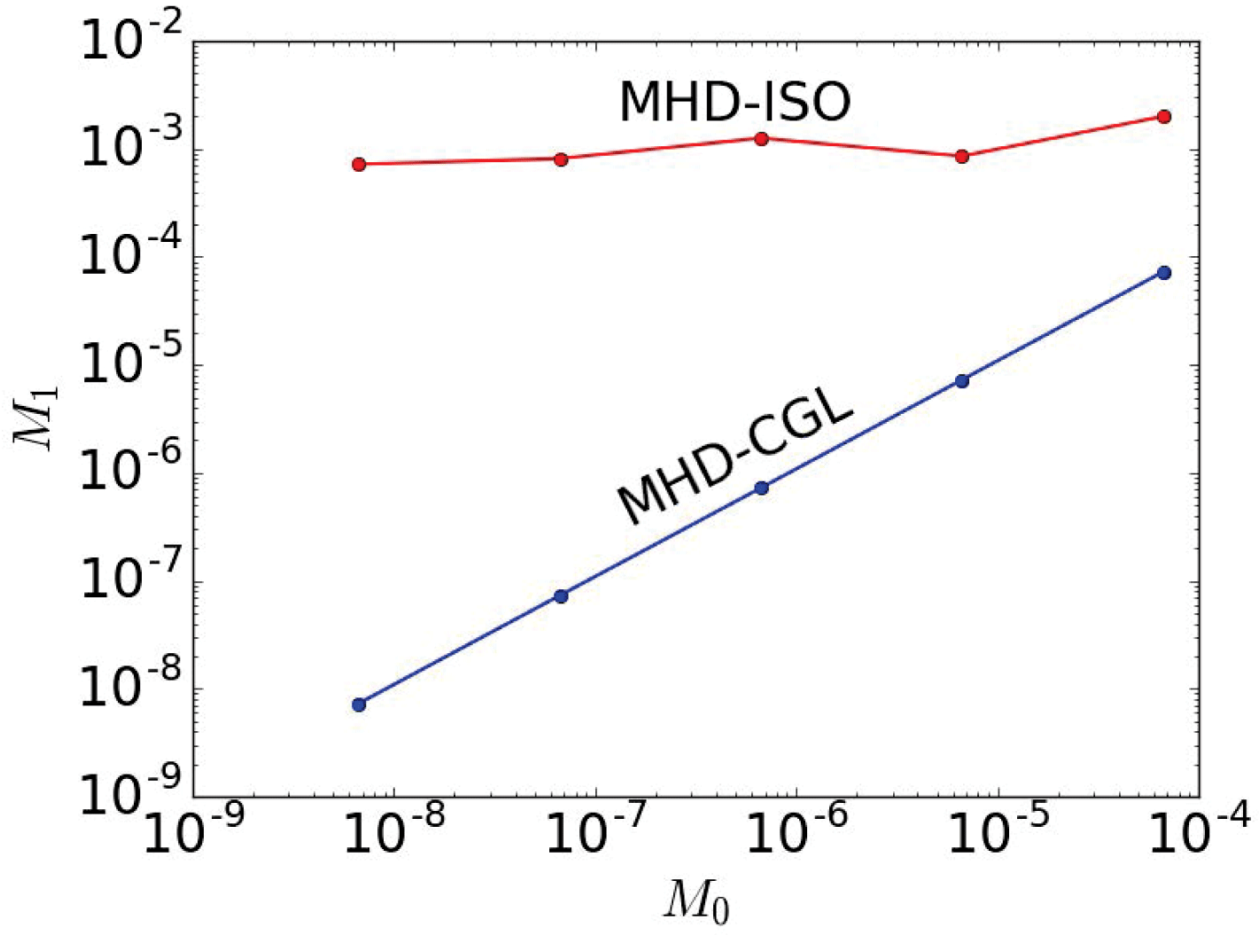
The saturated magnetic energy $M_{1}$ versus the initial one $M_{0}$ for the MHD (red) and CGL (blue) models.

Figure 3 shows the evolution of the magnetic energy for the two models in simulations starting from the magnetic-field strength $B_{0}$ corresponding to the range $10^{4}<\unicode[STIX]{x1D6FD}_{0}<10^{8}$ . The amplitude of the forcing and the thermal pressure are the same for all these simulations, implying approximately the same Mach number of the velocity fluctuations in all of them. We see that the saturated magnetic energy is essentially independent of $\unicode[STIX]{x1D6FD}_{0}$ in the MHD model and entirely determined by it in the CGL model. This point is reinforced by figure 4, which shows the final saturated magnetic energy $M_{1}$ vs. the initial one $M_{0}$ . Thus, the initial magnetic energy cannot be increased in a double-adiabatic, pressure-anisotropic plasma even in the presence of external forcing and the upper bound (2.38) is tight.