





1 Introduction
1.1 Bounded geodesics on complete Riemannian manifolds
Let M be a complete Riemannian manifold and let
$S(M)$
 denote its unit tangent bundle, whose fiber
$S_p(M)$
 over a point
$p\in M$
 is the unit sphere in
$T_p(M)$
 centered at the origin. For any
$p\in M$
 and any
$\xi \in S_p(M)$
 , let
$\gamma (p,\xi )$
 denote the geodesic ray through the base point p in the direction
$\xi $
 . Of particular interest is the following subset of
$S(M)$
 :

and its section over a point
$p\in M$
 :

It is trivial to see that
$E^+(\infty )=S(M)$
 when M itself is compact. However, for a general non-compact complete Riemannian manifold M, it is not even clear whether
$E^+(\infty )$
 is non-empty. One can find in [Reference Schroeder37] an affirmative answer for a complete Riemannian manifold with
$\dim (M)\geq 3$
 , curvature bounded by
$[-b^2,-1]$
 for some
$b>1$
 and finite volume.
In fact, one can say more for the special case when M is a locally symmetric space of non-compact type with finite Riemannian volume. Here and hereafter, we say that a subset E in a metric space S is thick if
$\dim (E\cap U)=\dim (U)$
 for any open subset U of S, where
$\dim $
 stands for the Hausdorff dimension on S. Dani [Reference Dani20] proved in the 1980s that
$E^+(\infty )$
 is thick in
$S(M)$
 for M as above with a constant negative curvature (in particular of rank
$1$
 ). A decade later, Aravinda and Leuzinger [Reference Aravinda7, Reference Aravinda and Leuzinger8] proved that each
$E^+(p,\infty )$
 has the winning property for Schmidt’s game (see §2) when restricted to a non-constant
$C^1$
 curve, and hence, is thick in
$S_p(M)$
 for M as above of rank
$1$
 . Similar results were also proved for the Teichmuller geodesic flow on the moduli space of unit-area holomorphic quadratic differentials by Kleinbock and Weiss [Reference Kleinbock and Weiss26] and by Chaika, Cheung, and Masur [Reference Chaika, Cheung and Masur18].
In this paper, we first generalize the previous results as follows.
Theorem 1.1. Let M be a locally symmetric space of non-compact type with finite Riemannian volume. Then, for any
$p\in M$
 , the set
$E^+(p,\infty )$
 is thick in
$S_p(M)$
 .
We remark here that Theorem 1.1 easily follows from [Reference Kleinbock and Margulis25, Corollary 5.5] and Marstrand slicing theorem. See §3 for details of the proof.
The main point of this paper is to consider a stronger property of sets than thickness. In the 1960s, Schmidt [Reference Schmidt36] introduced a certain game played on any metric space, where a winning set for this game is proved to be thick. Later, Schmidt’s winning property was upgraded to an even stronger hyperplane absolute winning property (abbreviated as HAW) by Broderick et al [Reference Broderick, Fishman, Kleinbock, Reich and Weiss15] on any Euclidean space, and by Kleinbock and Weiss [Reference Kleinbock and Weiss29] on any
$C^1$
 manifold. It should be stressed here that for any winning property mentioned previously, it has the advantage that any countable intersection of winning sets is still winning. See §2 for all definitions and discussions, and [Reference An1–Reference An, Guan and Kleinbock6, Reference Badziahin, Pollington and Velani9–Reference Broderick, Fishman and Kleinbock14, Reference Broderick, Fishman and Simmons16, Reference Kleinbock and Weiss27, Reference Kleinbock and Weiss28, Reference Nesharim and Simmons33] for other recent results involving winning properties of exceptional sets in Diophantine approximations and dynamical systems.
In this terminology, we raise a stronger conjecture than Theorem 1.1.
Conjecture 1.2. Let M be a locally symmetric space of non-compact type with finite Riemannian volume. Then, for any
$p\in M$
 , the set
$E^+(p,\infty )$
 is HAW on
$S_p(M)$
 .
Now, we briefly review some basic facts concerning locally symmetric spaces. Let M be a locally symmetric space of non-compact type and let
$\widetilde {M}$
 denote its universal cover. The isometry group G of
$\widetilde {M}$
 has finitely many connected components, whose identity component is a connected semisimple Lie group without compact factors and with trivial center. Fix a point
$p_0\in M$
 and let
$\widetilde {p_0}\in \widetilde {M}$
 be a preimage of
$p_0$
 . The stabilizer
$K:=\mathrm {Stab}_G(\widetilde {p_0})$
 is a maximal compact subgroup of G. We identify the globally symmetric space
$\widetilde {M}$
 with
$K\backslash G$
 and view the fundamental group
$\Gamma :=\pi _1(M)$
 as a torsion-free discrete subgroup of G via deck transformations. Then, M can be identified with
$K\backslash G/\Gamma $
 . Conversely, given any semisimple Lie group G without compact factors and with finite center, any maximal compact subgroup
$K\subset G$
 , and any torsion-free discrete subgroup
$\Gamma \subset G$
 , there exists a unique locally symmetric space structure on
$K\backslash G/\Gamma $
 . Moreover, M has finite Riemannnian volume if and only if
$\Gamma $
 is a lattice in G, and the rank of M is the rank of G.
In this paper, we verify Conjecture 1.2 for a special kind of locally symmetric space of non-compact type with finite Riemannian volume and of rank
$2$
 .
Theorem 1.3. Let
$G=\mathrm {SL}_{3}(\mathbb {R}),K=\mathrm {SO}_3(\mathbb {R})$
 ,
$\Gamma \leq G$
 be a torsion-free subgroup commensurable with
$\mathrm {SL}_3(\mathbb {Z})$
 , and
$Y=K\backslash G/\Gamma $
 be endowed with the above natural locally symmetric space structure. Then, Conjecture 1.2 holds for Y, that is, for any
$y\in Y$
 , the set
$E^+(y,\infty )$
 is HAW on
$S_y(Y)$
 .
1.2 Relations between homogeneous dynamics and geometry
Theorem 1.3 can also be reinterpreted from the view of homogeneous dynamics. Let G be a semisimple Lie group without compact factors and with finite center,
$\Gamma \subseteq G$
 be a non-uniform torsion-free lattice, and
$X=G/\Gamma $
 be the corresponding homogeneous space. Then, for any maximal compact subgroup K of G, there exists a proper projection

which realizes a locally symmetric space as the quotient of a homogeneous space with compact fiber.
Now write
$\mathfrak {g}=\mathrm {Lie}(G)$
 . There exists a Cartan involution
$\theta $
 with respect to the Killing form of
$\mathfrak {g}$
 , which induces a Cartan decomposition
$\mathfrak {g}=\mathfrak {k}\oplus \mathfrak {p}$
 . Here,
$\mathfrak {k}$
 and
$\mathfrak {p}$
 are the
$1$
 and
$-1$
 eigenspaces of
$\theta $
 , respectively. The involution
$\theta $
 also extends to an involutive automorphism
$\widetilde {\theta }$
 of G. Let
$K=G_{\widetilde {\theta }}$
 denote the subgroup of all
$\widetilde {\theta }$
 -fixed elements in G. Then, K is a maximal compact subgroup of G and there is a diffeomorphism

It follows that the differential at
$1_G$
 of the projection
$G\to K\backslash G$
 gives a linear isomorphism

By homogeneity, the tangent space of each point
$[Kg]\in K\backslash G$
 is isomorphic to
$\mathfrak {p}$
 . Moreover, the Riemannian metric on it can be seen as the
$\mathrm {Ad}(K)$
 -invariant inner product on
$\mathfrak {p}$
 . Then, the unit tangent space equals
$\mathfrak {p}^1:=\{\mathbf {v}\in \mathfrak {p}: \|\mathbf {v}\|=1\}$
 .
For each base point
$[Kg]\in K\backslash G$
 and each direction
$\xi =(\mathrm {d}R_g)(\mathbf {v})\in T_{[Kg]}(K\backslash G)$
 with
$\mathbf {v}\in \mathfrak {p}^1$
 , the associated geodesic ray on
$K\backslash G$
 is given by

Under the canonical covering map
$K\backslash G\to K\backslash G/\Gamma $
 , the tangent space of each point
${y=[Kg\Gamma ]\in Y}$
 can be identified with that of
$[Kg]\in K\backslash G$
 , and each geodesic ray in Y through the base point y in the direction
$\xi $
 can be written as

It follows that

This reduces Theorem 1.3 into the framework of homogeneous dynamics. Since any countable intersection of HAW sets is still HAW and, hence, thick in the ambient space, we immediately get the following corollary of Theorem 1.3.
Corollary 1.4. Let
$G,\Gamma ,K,\mathfrak {p},Y$
 be as in Theorem 1.3. Then, for any countably many points
$\{y_n=[Kg_n\Gamma ]\}_{n\in \mathbb {N}}$
 in Y, the set

is thick in
$\mathfrak {p}^1$
 .
One can also consider all bounded diagonal rays through a point on the homogeneous space
$X=G/\Gamma $
 . Let

denote the positive projective space of
$\mathfrak {g}$
 . For each point
$x\in X$
 , we write

The counterparts of Theorem 1.1, Conjecture 1.2, Theorem 1.3, and Corollary 1.4 are as follows.
Theorem 1.5. Let G be a Lie group,
$\Gamma \subseteq G$
 be a lattice, and
$X=G/\Gamma $
 be the corresponding homogeneous space. Then, for any
$x\in X$
 , the set
$E^+(x,\infty )$
 is thick in
$\mathbf {P}^+(\mathfrak {g})$
 .
Conjecture 1.6. Let G be a Lie group,
$\Gamma \subseteq G$
 be a lattice, and
$X=G/\Gamma $
 be the corresponding homogeneous space. Then, for any
$x\in X$
 , the set
$E^+(x,\infty )$
 is HAW on
$\mathbf {P}^+(\mathfrak {g})$
 .
Theorem 1.7. Let
$G=\mathrm {SL}_{3}(\mathbb {R}),\Gamma =\mathrm {SL}_{3}(\mathbb {Z})$
 , and
$X= G/\Gamma $
 be the corresponding homogeneous space. Then, Conjecture 1.6 holds for X, that is, for any
$x\in X$
 , the set
$E^+(x,\infty )$
 is HAW on
$\mathbf {P}^+(\mathfrak {g})$
 .
Corollary 1.8. Let
$G,\Gamma ,\mathfrak {g},X$
 be as in Theorem 1.7. Then, for any countably many points
$\{x_n\}_{n\in \mathbb {N}}$
 in X, the set

is thick in
$\mathbf {P}^+(\mathfrak {g})$
 .
Remark 1.9. Moreover, Conjectures 1.2 and 1.6 also hold for
$G=\prod _{i=1}^s\mathrm {SL}_2(\mathbb {R})$
 with a lattice
$\Gamma $
 and a maximal compact subgroup K in G. This can be done by combining the arguments in this paper and [Reference An, Ghosh, Guan and Ly4].
1.3 Organization of the paper and strategy of the proof
The paper is organized as follows. In §2, we recall the definitions and properties of Schmidt’s game and its variants—the hyperplane absolute game and the hyperplane potential game. In §3, we directly prove Theorems 1.1 and 1.5 by combining [Reference Kleinbock and Margulis25, Corollary 5.5] and Marstrand slicing theorem. In §4, we state our key result Theorem 4.1, from which we deduce Theorems 1.3 and 1.7. The proof of Theorem 4.1, which forms the most technical part of this paper, is given in §§5–7.
We highlight here that two of our main theorems, Theorems 1.1 and 1.3, are formulated in a purely geometric way. They can be viewed as applications of the corresponding results in the field of homogeneous dynamics.
Concerning the proof of Theorem 4.1, the target set (4.1) can be regarded as a fiber bundle over an open interval of weight parameters, where each fiber is proved to be HAW on its ambient space (see [Reference An, Guan and Kleinbock5]). We manage to show that the winning strategy is ‘locally constant’ with respect to the parameters, which is reflected in the choices of planes (7.5) in the proof of Lemma 5.5. This requires a detailed analysis of how the strategy used in [Reference An, Guan and Kleinbock5] depends on the weight parameter.
2 Preliminaries on Schmidt games
2.1 Schmidt’s
$(\alpha ,\beta )$
 -game

We first recall Schmidt’s
$(\alpha ,\beta )$
 -game introduced in [Reference Schmidt36]. It involves two parameters
$\alpha ,\beta \in (0,1)$
 , and is played by two players Alice and Bob on a complete metric space
$(X,\mathrm {dist})$
 with a target set
$S\subset X$
 . Bob starts the game by choosing a closed ball
$B_0=B(x_0,\rho _0)$
 in X with center
$x_0$
 and radius
$\rho _0$
 . After Bob chooses a closed ball
$B_i = B(x_i,{\rho }_i) $
 , Alice chooses
$A_i = B(x_i', {\rho }_i')$
 with

and then Bob chooses
$B_{i+1} = B(x_{i+1},{\rho }_{i+1}) $
 with

etc. This implies that the balls are nested:

Alice wins the game if the unique point
$\bigcap _{i=0}^\infty A_i=\bigcap _{i=0}^\infty B_i$
 belongs to S, and Bob wins otherwise. The set S is
$(\alpha ,\beta )$
 -winning if Alice has a winning strategy, is
$\alpha $
 -winning if it is
$(\alpha ,\beta )$
 -winning for any
$\beta \in (0,1)$
 , and is winning if it is
$\alpha $
 -winning for some
$\alpha $
 . Schmidt [Reference Schmidt36] proved that:
-
• winning subsets of Riemannian manifolds are thick;
-
• if S is $\alpha $
-winning and
$\varphi :X\to X$
is bi-Lipschitz, then
$\varphi (S)$
is
$\alpha '$
-winning, where
$\alpha '$
depends on
$\alpha $
and the bi-Lipschitz constant of
$\varphi $
; -
• a countable intersection of $\alpha $
-winning sets is again
$\alpha $
-winning.


As such, Schmidt’s game has been a powerful tool for proving thickness of intersections of certain countable families of sets, see e.g. [Reference An1, Reference An2, Reference Broderick, Bugeaud, Fishman, Kleinbock and Weiss13–Reference Broderick, Fishman, Kleinbock, Reich and Weiss15, Reference Dani20–Reference Dani22]. However, for a fixed
$\alpha $
 , the class of
$\alpha $
 -winning subsets of a Riemannian manifold depends on the choice of the metric, and is not known to be preserved by diffeomorphisms.
2.2 Hyperplane absolute game on
$\mathbb {R}^d$

Inspired by ideas of McMullen [Reference McMullen32], the hyperplane absolute game on the Euclidean space
$\mathbb {R}^d$
 was introduced in [Reference Broderick, Fishman, Kleinbock, Reich and Weiss15]. It has the advantage that the family of its winning sets is preserved by
$C^1$
 diffeomorphisms. Let
$S \subset \mathbb {R}^d$
 be a target set and let
$\beta \in (0, \tfrac 13 )$
 . As before, Bob begins by choosing a closed ball
$B_0$
 of radius
${\rho }_0$
 . For an affine hyperplane
$L\subset \mathbb {R}^d$
 and
$\rho>0$
 , we denote the
${\rho }$
 -neighborhood of L by

Now, after Bob chooses a closed ball
$B_i$
 of radius
${\rho }_i$
 , Alice chooses a hyperplane neighborhood
$L_i^{({\rho }^{\prime }_i)}$
 with
${\rho }^{\prime }_i\le \beta {\rho }_i$
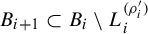
 , and then Bob chooses a closed ball
$B_{i+1}\subset B_i\setminus L_i^{({\rho }^{\prime }_i)}$
 of radius
${\rho }_{i+1}\ge \beta {\rho }_i$
 . Alice wins the game if and only if

The set S is
$\beta $
 -hyperplane absolute winning (
$\beta $
 -HAW for short) if Alice has a winning strategy, and is hyperplane absolute winning (HAW for short) if it is
$\beta $
 -HAW for any
${\beta \in (0,\tfrac 13)}$
 .
Lemma 2.1. [Reference Broderick, Fishman, Kleinbock, Reich and Weiss15]
-
(i) HAW subsets are winning and hence thick.
-
(ii) A countable intersection of HAW subsets is again HAW.
-
(iii) The image of a HAW set under a $C^1$
diffeomorphism
$\mathbb {R}^d \to \mathbb {R}^d$
is HAW.


2.3 HAW subsets of a manifold
The notion of HAW sets has been extended to subsets of
$C^1$
 manifolds in [Reference Kleinbock and Weiss29]. This is done in two steps. First, one defines the absolute hyperplane game on an open subset
$W \subset \mathbb {R}^d$
 . It is defined just as the absolute hyperplane game on
$\mathbb {R}^d$
 , except for requiring that Bob’s first move
$B_0$
 be contained in W. If Alice has a winning strategy, we say that S is HAW on W. Now, let M be a d-dimensional
$C^1$
 manifold and let
$\{(U_\alpha , \varphi _\alpha )\}$
 be a
$C^1$
 -atlas, that is,
$\{U_\alpha \}$
 is an open cover of M and each
$\varphi _\alpha $
 is a
$C^1$
 diffeomorphism from
$U_\alpha $
 onto the open subset
$\varphi _\alpha (U_\alpha )$
 of
$\mathbb {R}^d$
 . A subset
$S\subset M$
 is said to be HAW on M
if for each
$\alpha $
 ,
$\varphi _\alpha (S\cap U_\alpha )$
 is HAW on
$\varphi _\alpha (U_\alpha )$
 . Note that Lemma 2.1(iii) implies that the definition is independent of the choice of the atlas (see [Reference Kleinbock and Weiss29] for details).
Lemma 2.2. [Reference Kleinbock and Weiss29]
-
(i) HAW subsets of a $C^1$
manifold are thick. -
(ii) A countable intersection of HAW subsets of a $C^1$
manifold is again HAW. -
(iii) Let $\varphi :M\to N$
be a diffeomorphism between
$C^1$
manifolds and let
$S\subset M$
be a HAW subset of M. Then,
$\varphi (S)$
is a HAW subset of N. -
(iv) Let M be a $C^1$
manifold with an open cover
$\{U_\alpha \}$
. Then, a subset
$S\subset M$
is HAW on M if and only if
$S\cap U_\alpha $
is HAW on
$U_\alpha $
for each
$\alpha $
. -
(v) Let $M, N$
be
$C^1$
manifolds and let
$S\subset M$
be a HAW subset of M. Then,
$S\times N$
is a HAW subset of
$M\times N$
.





Proof. Items (i)–(iii) appeared as [Reference Kleinbock and Weiss29, Proposition 3.5] and are clear from Lemma 2.1. Item (iv) is clear from the definition. Item (v) is proved in [Reference Kleinbock and Weiss29, Proof of Theorem 3.6(a)].
We shall also need the following lemma.
Lemma 2.3. Let M be a
$C^1$
 manifold of dimension d,
$M'\subset M$
 be a finite union of
$C^1$
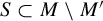
 submanifolds of strict lower dimensions. Then,
$S\subset M\setminus M'$
 is HAW on
$M\setminus M'$
 if and only if it is HAW on M.
Proof. The if direction is a direct consequence of the definition. For the only if direction, by using an induction argument, we may assume that
$M'$
 itself is a
$C^1$
 submanifold of strict lower dimension. We choose and fix a
$C^1$
 -atlas
$\{(U_\alpha ,\phi _\alpha )\}$
 of M such that, for any
$\alpha $
 , there exists a hyperplane
$L_{\alpha }\subset \mathbb {R}^d$
 satisfying

Since the HAW property is independent of choices of the atlas, to prove S is HAW on M, it suffices to prove
$\phi _{\alpha }(S\cap U_\alpha )$
 is HAW on
$\phi _{\alpha }(U_{\alpha })$
 for all
$U_\alpha $
 in this specific
$C^1$
 -atlas. As
$\{(U_\alpha \cap (M\setminus M'),\phi _\alpha )\}$
 is a
$C^1$
 -atlas of
$M\setminus M'$
 ,
$\phi _{\alpha }(S\cap U_\alpha \cap (M\setminus M'))$
 is HAW on
$\phi _{\alpha }(U_{\alpha }\cap (M\setminus M'))$
 . In view of these properties, the winning strategy for Alice is clear: for any
$\beta $
 -hyperplane absolute game played on
$\phi _{\alpha }(U_{\alpha })$
 , after Bob chooses his
$B_0$
 , Alice chooses neighborhood
$L_{\alpha }^{\beta \rho (B_0)}$
 as her first move. Then, the rest of the game is played on
$\phi _{\alpha }(U_{\alpha }\cap (M\setminus M'))$
 , so Alice can play according to her winning strategy on this set. This completes the proof.
2.4 Hyperplane potential game
Finally, we recall the hyperplane potential game introduced in [Reference Fishman, Simmons and Urbański23]. Being played on
$\mathbb {R}^d$
 , it has the same winning sets as the hyperplane absolute game. This allows one to prove the HAW property of a set
$S\subset \mathbb {R}^d$
 by showing that it is winning for the hyperplane potential game (see [Reference Nesharim and Simmons33]).
Let
$S\subset \mathbb {R}^d$
 be a target set and let
$\beta \in (0,1)$
 ,
$\gamma>0$
 . The
$(\beta ,\gamma )$
 -hyperplane potential game is defined as follows. Bob begins by choosing a closed ball
$B_0\subset \mathbb {R}^d$
 . After Bob chooses a closed ball
$B_i$
 of radius
${\rho }_i$
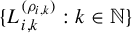
 , Alice chooses a countable family of hyperplane neighborhoods
$\{L_{i,k}^{({\rho }_{i,k})} : k\in \mathbb {N}\}$
 such that

and then Bob chooses a closed ball
$B_{i+1}\subset B_i$
 of radius
$\rho _{i+1}\ge \beta \rho _i$
 . Alice wins the game if and only if

The set S is
$(\beta ,\gamma )$
 -hyperplane potential winning (
$(\beta ,\gamma )$
 -HPW for short) if Alice has a winning strategy, and is hyperplane potential winning (HPW for short) if it is
$(\beta ,\gamma )$
 -HPW for any
$\beta \in (0,1)$
 and
$\gamma>0$
 . The following lemma is a special case of [Reference Fishman, Simmons and Urbański23, Theorem C.8].
Lemma 2.4. A subset
$S\subset \mathbb {R}^d$
 is HPW if and only if it is HAW.
3 Proof of Theorems 1.1 and 1.5
In this section, we prove Theorems 1.1 and 1.5 by reducing them to [Reference Kleinbock and Margulis25, Corollary 5.5]. For the sake of convenience, we state one version of the aforementioned result here.
Theorem 3.1. [Reference Kleinbock and Margulis25, Corollary 5.5]
Let G be a Lie group,
$\Gamma $
 be a lattice in G, F be a one-parameter
$\mathrm {Ad}$
 -diagonalizable subgroup of G,
$H=H(F^+)$
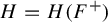 be the unstable horospherical subgroup with respect to
$F^+$
 , and
$X=G/\Gamma $
 . Then, for any
$x\in X$
 , the set

is thick in H.
Proof of Theorem 1.1
We first recall some notation in §1. Let M be a locally symmetric space of non-compact type with finite Riemannian volume. Then, M can be identified with
$Y=K\backslash G/\Gamma $
 , where G is a semisimple Lie group without compact factors and with finite center, K is a maximal compact subgroup of G, and
$\Gamma $
 is a lattice in G. Let
$X=G/\Gamma $
 ,
$\mathfrak {g}=\mathrm {Lie}(G),\mathfrak {k}=\mathrm {Lie}(K)$
 , and
$\mathfrak {p}\subset \mathfrak {g}$
 be the orthogonal complement of
$\mathfrak {k}$
 . Then, it suffices to show that: for any point
$y=[Kg\Gamma ]\in Y$
 , the set

is thick in
$\mathfrak {p}^1$
 .
Let us choose a maximal abelian subspace
$\mathfrak {a}\subset \mathfrak {p}$
 and an open Weyl chamber
$\mathfrak {a}_+\subset \mathfrak {a}$
 . Let
$L=Z_K(\mathfrak {a})$
 and
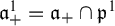
$\mathfrak {a}^1_+=\mathfrak {a}_+\cap \mathfrak {p}^1$
 . Then, the map

is a diffeomorphism onto an open dense subset of
$\mathfrak {p}^1$
 . Then, it suffices to prove that the set

is thick in
$\mathfrak {a}^1_+\times L\backslash K$
 . Moreover, by Marstrand’s slicing and projection theorems [Reference Marstrand30], we only need to prove that: for any
$\mathbf {v}\in \mathfrak {a}^1_+$
 , the set

is thick in K, since the set (3.1) can be decomposed into a union of slices, each of which is a quotient of a set of the form (3.2).
Let
$F_{\mathbf {v}}^+=\{\exp (t\mathbf {v}): t\geq 0\}$
 be the one-parameter subsemigroup of G, and
$H=H(F_{\mathbf {v}}^+)$
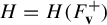 (respectively
$H^0=H^0(F_{\mathbf {v}}^+),H^-=H^-(F_{\mathbf {v}}^+)$
 ) be the unstable (respectively neutral, stable) horospherical subgroup with respect to
$F_{\mathbf {v}}^+$
 . Let
$B=H^0H$
 and
$B^-=H^-H^0$
 , and consider the action of the subgroup K on the real flag variety
$G/B$
 by left translation. By Iwasawa decomposition, this action is transitive. It follows that for any
$g\in G$
 , the map

is a projection map with compact fiber. Write
$K'=K\cap B^-Bg^{-1}=K\cap B^-Hg^{-1}$
 . Then,
$K\setminus K'=\phi _g^{-1}((G\setminus B^{-1}B)/B)$
 is a finite union of manifolds of strict lower dimensions. So, it suffices to show that
$E_K^+([g\Gamma ],\infty )\cap K'$
 is thick in
$K'$
 .
For
$k\in K'$
 , we set
$\sigma _1(k)\in B^-$
 and
$\sigma _2(k)\in H$
 to be the unique pair satisfying
${kg=\sigma _1(k)\sigma _2(k)}$
 . It is easy to check that the map
$\sigma _2$
 is a projection map. However,

Consequently,

In view of Theorem 3.1, we see that
$E_H^+([1_G\Gamma ],\infty )$
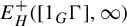 is thick in H and, hence, by Marstrand’s slicing theorem,
$E_K^+([g\Gamma ],\infty )\cap K'$
 is thick in
$K'$
 . This completes the proof.
Proof of Theorem 1.5
We begin with a simple observation, that is, it suffices to prove Theorem 1.7 for
$x=[1_G\Gamma ]\in X$
 . Indeed, for any
$x'=[g\Gamma ]\in X$
 and one-parameter subgroup
$F\subset G$
 ,
$F^+x'$
 is bounded if and only if
$g^{-1}F^+gx$
 is bounded, which implies

Thus, it suffices to prove Theorem 1.5 for
$x=[1_G\Gamma ]\in X$
 .
Let
$p:\mathfrak {g}\setminus \{0\}\to \mathbf {P}^+(\mathfrak {g})$
 denote the projection map. By Marstrand’s projection and slicing theorems, to prove Theorem 1.5 is equivalent to show that the set

is thick in
$\mathfrak {g}$
 . We claim that we may reduce to the case when G is a connected semisimple Lie group with trivial center and without compact factors for the following reasons.
First, let
$G^0$
 denote the identity component of G. It is clear that
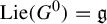
$\mathrm {Lie}(G^0)=\mathfrak {g}$
 and that
$X^0=G^0/(G^0\cap \Gamma )$
 is a connected component of X containing
$[1_G\Gamma ]$
 . In particular,

So, we may assume that
$G=G^0$
 is connected without loss of generality.
Second, let
$\mathfrak {g}=\mathfrak {r}\rtimes \mathfrak {l}$
 be the Levi decomposition, where
$\mathfrak {r}$
 is the solvable radical of
$\mathfrak {g}$
 and
$\mathfrak {l}$
 is a Levi subalgebra of
$\mathfrak {g}$
 . Let
$\mathfrak {l}=\mathfrak {l}_c\oplus \mathfrak {l}_{nc}$
 be the decomposition into simple ideals where
$\mathfrak {l}_c$
 is the direct sum of all compact simple ones. The projection map
$\mathrm {d}q:\mathfrak {g}\to \mathfrak {l}_{nc}$
 is a Lie algebra homomorphism, which induces a Lie group homomorphism
$q:G\to L_{nc}$
 and a projection map
$X=G/\Gamma \to X_{nc}:=L_{nc}/q(\Gamma )$
 . Note that
$q(\Gamma )$
 is a lattice in
$L_{nc}$
 , and the fiber of
$X\to X_{nc}$
 is a compact homogeneous space
$RL_c/(RL_c\cap \Gamma )$
 (see [Reference Dani19, Lemma 9.1]). Then, for
$\mathbf {v}\in \mathfrak {g}$
 ,

It follows that

By Marstrand’s slicing theorem, it suffices to show that

is thick in
$\mathfrak {l}_{nc}$
 . So, we may assume that G is a semisimple Lie group without compact factors.
Finally, since
$X=G/\Gamma $
 is a finite cover of
$G/(Z(G)\cdot \Gamma )$
 , we may replace G by
$G/Z(G)$
 and
$\Gamma $
 by
$(\Gamma \cdot Z(G))/Z(G)$
 without loss of generality. These verify the claim.
Now, let G be a connected semisimple Lie group with trivial center and without compact factors. Let
$G=K\cdot \exp (\mathfrak {p})$
 be the global Cartan decomposition,
$\mathfrak {a}\subset \mathfrak {p}$
 be a maximal abelian subspace, and
$L=Z_K(\mathfrak {a})$
 . We choose an open Weyl chamber
$\mathfrak {a}_+\subset \mathfrak {a}$
 , and for any
$\mathbf {v}\in \mathfrak {a}_+$
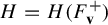
 , let
$H=H(F_{\mathbf {v}}^+)$
 (respectively
$H^0=H^0(F_{\mathbf {v}}^+),H^-=H^-(F_{\mathbf {v}}^+)$
 ) be the unstable (respectively neutral, stable) horospherical subgroup with respect to
$F_{\mathbf {v}}^+$
 . Note that the subgroups
$H,H^0,H^-$
 only depend on the choice of the open Weyl chamber
$\mathfrak {a}_+$
 .
Consider the map

It is easy to check that
$\theta $
 is a diffeomorphism onto
$\mathfrak {g}$
 . Using Bruhat decomposition, there is a diffeomorphism onto its image:

It follows that the composition map

is also a diffeomorphism onto its image. Moreover, we see that p is a projection map when restricted to
$\mathrm {Im}(\theta )$
 and that
$\mathfrak {g}\setminus \mathrm {Im}\ \theta $
 is a finite union of submanifolds of strict lower dimensions. Thus, it suffices to prove that

is thick on
$\mathfrak {a}_+\times H\times L\times H^-$
 . However, we have for any
$\mathbf {v}\in \mathfrak {a}_+$
 ,

So, the conclusion follows from Marstrand’s slicing theorem and Theorem 3.1. This completes the proof.
4 Proof of Theorems 1.3 and 1.7
In this section, we prove Theorems 1.3 and 1.7 by assuming the truth of Theorem 4.1 in the following. The proof of Theorem 4.1 will be postponed to the next section.
For any
$\unicode{x3bb} \in \Pi :=(1/2,1)$
 , set

Let
$ U\subset G$
 (respectively
$U^- \subset G$
 ) be the subgroup of unipotent upper triangular (respectively lower triangular) matrices and
$A\subset G$
 be the subgroup of diagonal matrices with positive entries. Then, U (respectively
$U^-$
 ) is the expanding (respectively contracting) subgroup of
$F_{\unicode{x3bb} }^+$
 for any
$\unicode{x3bb} \in \Pi $
 . Define

Both Theorems 1.3 and 1.7 will be deduced from the following theorem.
Theorem 4.1. The set

is HAW on
$\Pi \times U$
 .
Remark 4.2. In [Reference An, Guan and Kleinbock5], it is proved that
$E_U(F_{\unicode{x3bb} }^+)$
 is HAW on U for any
$\unicode{x3bb} \in \Pi $
 . However, Theorem 4.1 does not follow from this result. It is generally believed that for a general Borel subset in a product space, winning properties of all its slices do not necessarily imply the winning property of itself.
Proof of Theorem 1.3 modulo Theorem 4.1
We first recall basic facts about geodesic flows on Y from [Reference Mautner31]. Let
$\mathfrak {k}=\mathrm {Lie}(K)$
 and
$\mathfrak {p}\subset \mathfrak {g}$
 be its orthogonal complement. Then, for any
$y=[Kg\Gamma ]\in Y$
 ,
$S_y(Y)$
 can be identified with
$\mathfrak {p}^1=\{\mathbf {v}\in \mathfrak {p}: \|\mathbf {v}\|=1\}$
 . Moreover, for any
$y=[Kg\Gamma ]\in Y$
 and
$\mathbf {v}\in \mathfrak {p}^1$
 , the associated geodesic ray is given by

Since K is compact, we have

The proof of Theorem 1.3 will be given in two steps. To begin, we consider the map

It is easy to check that
$\mathfrak {p}^1\setminus (\mathrm {Im}\ \theta \cup -\mathrm {Im}\ \theta )$
 is a finite union of manifolds of strict lower dimension. Hence, in view of Lemma 2.3, it suffices to prove that
${E^+(y,\infty )\cap \pm \mathrm {Im}\ \theta }$
 is HAW on
$\pm \mathrm {Im}\ \theta $
 . By applying
$\overline {\tau }:X\rightarrow X$
 induced by the outer automorphism
${\tau (g)=(g^T)^{-1}}$
 defined on G, we get

Thus, it suffices to show
$E^+(y,\infty )\cap \mathrm {Im}\ \theta $
 is HAW on
$\mathrm {Im}\ \theta $
 for any
$y\in Y$
 . However, it is also easy to check that
$\theta $
 is a cover map. Hence, in view of Lemma 2.2(iii), it suffices to show that

is HAW on
$\Pi \times K$
 .
Let
$ B\subset G$
 (respectively
$B^- \subset G$
 ) be the subgroup of upper triangular (respectively lower triangular) matrices, and consider the action of the subgroup K on the real flag variety
$G/B$
 by left translations. By Iwasawa’s decomposition, this action is transitive and has finite stabilizer. It follows that for any
$g\in G$
 , the map
$\phi _g: K\rightarrow G/B$
 defined by
$\phi _g(k)= kgB$
 is a cover map. Write
$K'=K\cap B^-Bg^{-1}=K\cap B^-Ug^{-1}$
 . Then,
$K\setminus K'=\phi _g^{-1}((G\setminus B^{-1}B)/B)$
 is a finite union of manifolds of strict lower dimensions. Using Lemma 2.3 again, it suffices to show that
$E":=E'\cap (\Pi \times K')$
 is HAW on
$\Pi \times K'$
 . For
$k\in K'$
 , we set
$\sigma _1(k)\in B^-$
 and
$\sigma _2(k)\in U$
 to be the unique pair satisfying
$kg=\sigma _1(k)\sigma _2(k)$
 . It is easy to check that the map
$\sigma _2$
 is a cover map. However,

Consequently,
$E"=(\mathrm {Id}\times \sigma _2)^{-1}S$
 . Thus, in view of Lemma 2.2(iii) and Theorem 4.1, we see that
$E"$
 is HAW on
$\Pi \times K'$
 . This completes the proof.
Proof of Theorem 1.7 modulo Theorem 4.1
We begin with a simple observation, that is, it suffices to prove Theorem 1.7 for
$x=[1_G\Gamma ]\in X$
 . Indeed, for any
$x'=[g\Gamma ]\in X$
 and one-parameter subgroup
$F\subset G$
 ,
$Fx'$
 is bounded if and only if
$g^{-1}Fgx$
 is bounded, which implies

Hence, in view of Lemma 2.2(iii), it suffices to prove Theorem 1.7 for
$x=[1_G\Gamma ]\in X$
 .
Consider the map

It is straightforward to check that the map
$\theta $
 is a diffeomorphism onto its image. Let p be the projection from
$\mathfrak {g}\setminus \{0\}$
 to
$\mathbf {P}^+(\mathfrak {g})$
 . Then, it can be checked that p is a diffeomorphism onto its image when restricted on
$\mathrm {Im}\ \theta \cup -\mathrm {Im}\ \theta$
 and
$\mathbf {P}^+(\mathfrak {g})\setminus (p(\mathrm {Im}\ \theta )\cup -p(\mathrm {Im}\ \theta ))$
 is a finite union of submanifolds of strict lower dimensions. In view of Lemmas 2.2(iv) and 2.3, it suffices to show that
$E^+([1_G\Gamma ],\infty )\cap \pm p(\mathrm {Im}\ \theta )$
 is HAW on
$\pm p(\mathrm {Im}\ \theta )$
 , respectively. Set

Then,
$E^+([1_G\Gamma ],\infty )=p(E^+(\infty )\setminus \{0\})$
 . We claim that Theorem 1.7 can be deduced from the following statement:

Indeed, on one hand, it follows from Lemma 2.2(iii) and (4.2) that

On the other hand, by applying the map
$\overline {\tau }:X\to X$
 induced by the outer automorphism
$\tau (g)=(g^T)^{-1}$
 defined on G, we see that

It follows again from Lemma 2.2(iii) and (4.2) that

These verify our claim.
Finally, to prove (4.2), it suffices to establish the HAW property of
$\theta ^{-1} (E^+(\infty ))$
 on
$\Pi \times U\times U^-$
 . However, we have

which means that
$\theta ^{-1} (E^+(\infty ))=S\times U^-$
 . So, the conclusion follows from Lemma 2.2(v) and Theorem 4.1. This completes the proof.
5 Proof of Theorem 4.1
In this section, we prove Theorem 4.1 modulo two key lemmas.
For
$(x,y,z)\in \mathbb {R}^3$
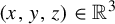 , set

For technical reasons, we will prove Theorem 4.1 by applying Lemma 2.2(iii) to the diffeomorphism
$\Psi :\Pi \times \mathbb {R}^3\to \Pi \times U$
 defined by

For simplicity, we write

It is directly checked that

So, it suffices to prove
$\Psi ^{-1}(S)$
 is HAW on
$\Sigma $
 .
For
$\unicode{x3bb} \in \Pi $
 ,
$\epsilon>0$
 , and
$\mathbf {v}=(p,r,q)\in \mathbb {Z}^2\times \mathbb {N}$
 , we set

and

Note that if
$\mathbf {v}'=t\mathbf {v} $
 with
$t>1$
 , then
$\Delta _\unicode{x3bb} (\mathbf {v}',\epsilon )\subset \Delta _\unicode{x3bb} (\mathbf {v},\epsilon )$
 . Thus,

Moreover, we set

According to [Reference An, Guan and Kleinbock5, Lemma 3.2], we know that
$\{\unicode{x3bb} \}\times S_\unicode{x3bb} (\epsilon )\subset \Psi ^{-1}(S)$
 for any
$\unicode{x3bb} \in \Pi $
 and
$\epsilon>0$
 . Hence,
$S(\epsilon )\subset \Psi ^{-1}(S)$
 for any
$\epsilon>0$
 . Therefore, Theorem 4.1 can be deduced from the following lemma.
Lemma 5.1. The set

is HAW on
$\Sigma $
 .
The rest of this section is devoted to the proof of Lemma 5.1. For convenience, we endow
$\Sigma $
 with the product metric. For a closed ball
$\Omega \subset \Sigma $
 , we denote its radius as
$\rho _{\Omega }$
 and its center as
$(\unicode{x3bb} _\Omega , \omega _\Omega )$
 with
$\unicode{x3bb} _\Omega \in \Pi ,\;\omega _\Omega =(x_\Omega , y_\Omega , z_\Omega )\in \mathbb {R}^3$
 . Hence, we have

Here,
$I(\unicode{x3bb} _\Omega ,\rho _\Omega )$
 and
$B(\omega _\Omega , \rho _\Omega )$
 denote the closed balls in
$\Pi $
 and
$\mathbb {R}^3$
 , respectively.
For a closed ball
$\Omega \subset \Sigma $
 and
$\mathbf {v}=(p,r,q)\in \Xi $
 , consider the set of integral vectors

It follows from Minkowski’s linear forms theorem that
$\mathcal {W}(\Omega ,\mathbf {v})\ne \varnothing $
 . We choose and fix

such that

and define

Lemma 5.2. For any closed ball
$\Omega \subset \Sigma $
 and
$\mathbf {v}=(p,r,q)\in \Xi $
 , we have

Proof. The first inequality is obvious. By Minkowski linear forms theorem,
$\mathcal {W}(\Omega ,\mathbf {v})$
 contains a vector
$(a_0,b_0,c_0)$
 with
$|a_0|\le q^{\unicode{x3bb} _\Omega }$
 and
$|b_0+z_\Omega a_0|\le q^{1-\unicode{x3bb} _\Omega }$
 . Thus, it follows from (5.2) that

Hence, the second inequality.
Let
$\Omega _0\subset \Sigma $
 be a closed ball of radius
$\rho _0$
 . Then,
$\rho _0< 1/4$
 . Let
$\kappa>2$
 be such that

Let
$\beta \in (0,1)$
 , and R and
$\epsilon $
 be positive numbers such that

and

Let
$\mathscr {B}_0=\{\Omega _0\}$
 . For
$n\ge 1$
 , let
$\mathscr {B}_n$
 be the family of closed balls defined by

For a closed ball
$\Omega $
 , if

we define

where

Note that since
$R>\beta ^{-1}$
 , the families
$\mathscr {B}_n$
 are pairwise disjoint. So, (5.7) is satisfied for at most one integer n, and hence,
$\mathcal {V}_\Omega $
 is well defined. It follows from (5.3) that if
${\mathbf {v}=(p,r,q)\in \mathcal {V}_\Omega }$
 , then

Whenever (5.7) is satisfied, we also define

and

Lemma 5.3. If
$\Omega \in \mathscr {B}_n$
 , then
$\mathcal {V}_\Omega =\bigcup _{k=1}^{[{n}/{2}]}\mathcal {V}_{\Omega ,k}$
 .
Proof. In view of (5.8), it suffices to show that if
$k>[{n}/{2}]$
 , then
$\mathcal {V}_{\Omega ,k}=\varnothing $
 . Suppose to the contrary that
$\mathcal {V}_{\Omega ,k}\ne \varnothing $
 for some
$k>[{n}/{2}]$
 . Let
$(p,r,q)\in \mathcal {V}_{\Omega ,k}$
 . Then,

However,

which is a contradiction.
Next, we inductively define a subfamily
$\mathscr {B}^{\prime }_n$
 of
$\mathscr {B}_n$
 as follows. Let
$\mathscr {B}^{\prime }_0=\{\Omega _0\}$
 . If
$n\ge 1$
 and
$\mathscr {B}^{\prime }_{n-1}$
 has been defined, we let

The following two lemmas concerning
$\mathscr {B}^{\prime }_n$
 are key steps in the proof of Theorem 4.1. Their proofs are technical and postponed to the next two sections.
Lemma 5.4. Let
$n\ge 0$
 ,
$\Omega \in \mathscr {B}^{\prime }_n$
 , and
$\mathbf {v}=(p,r,q)\in \Xi $
 . If
$q^{1+\unicode{x3bb} _\Omega }\le 2H_{n+1}$
 , then
$\Delta (\mathbf {v}, \epsilon )\cap \Omega =\varnothing $
 .
Lemma 5.5. Let
$n\ge 0$
 ,
$\Omega \in \mathscr {B}^{\prime }_n$
 , and
$k\geq 1$
 . There exists an affine hyperplane
${L_k(\Omega )\subset \Sigma }$
 such that for any
$\Omega '\in \mathscr {B}_{n+k}$
 with
$\Omega '\subset \Omega $
 and any
$\mathbf {v}\in \mathcal {V}_{\Omega ',k}$
 , we have

We now prove Lemma 5.1 assuming the truth of Lemmas 5.4 and 5.5.
Proof of Lemma 5.1
By Lemma 2.4, it suffices to prove that
$S'$
 is HPW on
$\Sigma $
 . Let
${\beta \in (0,1)}$
 ,
$\gamma>0$
 . We prove that Alice has a strategy to win the
$(\beta ,\gamma )$
 -hyperplane potential game on
$\Sigma $
 with target set
$S'$
 . In the first round of the game, Bob chooses a closed ball
$\Omega _0\subset \Sigma $
 . By [Reference An, Guan and Kleinbock5, Remark 2.4], we may without loss of generality assume that Bob will play so that
$\rho _i:=\rho (\Omega _i)\to 0$
 . Let
$\kappa $
 and R be positive numbers satisfying (5.4) and (5.5). We also require that

Let
$\epsilon , \mathscr {B}_n, \mathcal {V}_\Omega , \mathcal {V}_{\Omega ,k}$
 , and
$\mathscr {B}^{\prime }_n$
 be as above. Then, Lemmas 5.3–5.5 hold. Let Alice play according to the following strategy. Suppose that
$i\ge 0$
 and Bob has chosen the closed ball
$\Omega _i$
 . If there is
$n\ge 0$
 such that

then Alice chooses the family of neighborhoods
$\{L_k(\Omega _i)^{(2R^{-(n+k)}\rho _0)}:k\in \mathbb {N}\}$
 , where
$L_k(\Omega _i)$
 are the hyperplanes given in Lemma 5.5. Otherwise, Alice makes an arbitrary move. Since
$\Omega _i\in \mathscr {B}_n$
 , we have that
$\rho _i>\beta R^{-n}\rho _0$
 . This, together with (5.10), implies that

So, Alice’s move is legal. We prove that this guarantees a win for Alice, that is, the unique point
$\mathbf {x}_\infty =(\unicode{x3bb} _\infty , \omega _\infty )$
 in
$\bigcap _{i=0}^\infty \Omega _i$
 lies in

where

There are two cases.
Case (1). Assume
$\mathcal {N}=\mathbb {N}\cup \{0\}$
 . For any
$\mathbf {v}=(p,r,q)\in \Xi $
 , there is n such that
${q^{2}\le 2H_{n+1}}$
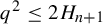 . Then, it follows that
$q^{1+\unicode{x3bb} _n}\le q^2\le 2H_{n+1}.$
 Since
$n\in \mathcal {N}$
 , we have that
$\Omega _{i_n}\in \mathscr {B}^{\prime }_n$
 . Then, Lemma 5.4 implies that
$\Delta (\mathbf {v},\epsilon )\cap \Omega _{i_n}=\varnothing $
 . Thus,
$\mathbf {x}_\infty \notin \Delta (\mathbf {v}, \epsilon )$
 . It then follows from (5.1) and the arbitrariness of
$\mathbf {v}$
 that
$\mathbf {x}_\infty \in S(\epsilon )\subset S'$
 . Hence, Alice wins.
Case (2). Assume
$\mathcal {N}\ne \mathbb {N}\cup \{0\}$
 . Let n be the smallest non-negative integer with
$n\notin \mathcal {N}$
 . Since
$B_0\in \mathscr {B}^{\prime }_0$
 , we have
$0\in \mathcal {N}$
 . Hence,
$n\ge 1$
 . Since
$\rho _i\to 0$
 and
$\rho _{i+1}\ge \beta \rho _i$
 , there must exist
$i\ge 1$
 with
$\Omega _i\in \mathscr {B}_n$
 and
$\Omega _{i-1}\notin \mathscr {B}_n$
 . It follows that
$\Omega _i\notin \mathscr {B}^{\prime }_n$
 . Since
$n-1\in \mathcal {N}$
 , we have
$\Omega _{i_{n-1}}\in \mathscr {B}^{\prime }_{n-1}$
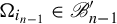 . Thus, it follows from (5.9) that
$\Omega _i\cap \bigcup _{\mathbf {v}\in \mathcal {V}_{\Omega _i}}\Delta (\mathbf {v},\epsilon )\ne \varnothing $
 . By Lemma 5.3, there is
$k\in [1,[n/2]]$
 and
$\mathbf {v}\in \mathcal {V}_{\Omega _i,k}$
 such that
${\Omega _i\cap \Delta (\mathbf {v}, \epsilon )\ne \varnothing }$
 . Applying Lemma 5.5 to
$\Omega =\Omega _{i_{n-k}}$
 and
$\Omega '=\Omega _i$
 , we obtain
$\Omega _i\cap \Delta (\mathbf {v},\epsilon )\subset L_k(\Omega _{i_{n-k}})^{(R^{-n}\rho _0)}$
 . So,
$\Omega _i\cap L_k(\Omega _{i_{n-k}})^{(R^{-n}\rho _0)}\ne \varnothing $
 . In view of
$\rho _i\le R^{-n}\rho _0$
 , it follows that
$\mathbf {x}_\infty \in \Omega _i\subset L_k(\Omega _{i_{n-k}})^{(2R^{-n}\rho _0)}$
 . Hence, Alice also wins.
This completes the proof of Theorem 4.1 modulo Lemmas 5.4 and 5.5.
6 Proof of Lemma 5.4
We shall need the following simple but useful lemma.
Lemma 6.1. Let
$n\ge 0$
 and
$\rho \in (0,R^{-n}\rho _0]$
 , then

Proof. The second inequality is straightforward. For the first inequality, the case
$n=0$
 is trivial since
$H_2<1$
 . Let
$n\geq 1$
 . Since the function
$x^{-1}\log x$
 is monotonically decreasing when
$x>e$
 , it follows that

This completes the proof of the first inequality.
Proof of Lemma 5.4
The case
$n=0$
 is trivial since
$2H_1<1$
 . Let
$n\geq 1$
 . We denote
${\Omega _n=\Omega }$
 and let
$\Omega _n\subset \cdots \subset \Omega _1\subset \Omega _0$
 be such that
$\Omega _k\in \mathscr {B}^{\prime }_k$
 . Write
$\unicode{x3bb} _{\Omega _k}=\unicode{x3bb} _k$
 and
${\rho _{\Omega _k}=\rho _k}$
 for simplicity. Suppose in contrast that the conclusion of the lemma is not true. Then, there exists
$\mathbf {v}=(p,r,q)\in \mathbb {Z}^2\times \mathbb {N}$
 with
$q^{1+\unicode{x3bb} _n}\le 2H_{n+1}$
 such that
${\Delta (\mathbf {v},\epsilon )\cap \Omega _k\ne \varnothing }$
 for every
$1\le k\le n$
 . It follows from the definition of
$\mathscr {B}^{\prime }_k$
 that
$\mathbf {v}\notin \mathcal {V}_{\Omega _k}$
 , that is,

Let
$1\le m\le n$
 be such that

We inductively prove that

By letting
$k=[{m}/{2}]$
 in (6.4), we have

which is a contradiction. So Lemma 5.4 follows from (6.4). Since

it follows from (6.2) that (6.4) holds for
$k=m$
 . Suppose that
$[{m}/{2}]\le k\le m-1$
 and (6.4) holds if k is replaced by
$k+1$
 . We prove that

To prove (6.5), the first step is to establish

Write
$\mathbf {w}(\Omega _k,\mathbf {v})=(a_k,b_k,c_k)$
 and
$z_{\Omega _k}=z_k$
 . Since
$\mathbf {w}(\Omega _{k+1},\mathbf {v})\in \mathcal {W}(\Omega _{k+1},\mathbf {v})$
 , we have

Note that
$\sqrt {\rho _{k+1}}\le \sqrt {\beta ^{-1} R^{-1}}\sqrt {\rho _k}\le ({1}/{10})\sqrt {\rho _k}$
 and by Lemma 6.1,

Now, we are in position to prove (6.6). First, we have

Second, we have

Hence, (6.6) holds. It then follows from (6.6) and the definition of
$\mathbf {w}(\Omega _k,\mathbf {v})$
 that

This proves (6.5).
It follows from (6.5) and the induction hypothesis that
$H_{\Omega _k}(\mathbf {v})< 2H_{k+1}$
 . By (6.2), we have
$H_{\Omega _k}(\mathbf {v})<H_k$
 . Thus, (6.4) is proved.
7 Proof of Lemma 5.5
In this section, we prove Lemma 5.5. We first establish the following lemma.
Lemma 7.1. Let
$n\ge 0$
 ,
$\Omega \in \mathscr {B}_n$
 , and
$\mathbf {v}=(p,r,q)\in \Xi $
 with
$q\le H_{2n+2}$
 . Then,

Proof. Let
$(\unicode{x3bb} ,x,y,z)\in \Delta (\mathbf {v},\epsilon )\cap \Omega $
 . Then,

Hence, to show (7.1), it suffices to show that, for any
$\unicode{x3bb} \in I_{\Omega }$
 ,
$q^{|\unicode{x3bb} -\unicode{x3bb} _{\Omega }|}\le 3$
 . According to Lemma 6.1, we have

This completes the proof.
Lemma 7.2. Let
$n\ge 0$
 ,
$\Omega \in \mathscr {B}^{\prime }_n$
 ,
$k\geq 1$
 , and
$\Omega _j\in \mathscr {B}_{n+k}$
 with
$\Omega _j\subset \Omega $
 ,
$j=1,2$
 . Let
$\mathbf {v}_j=(p_j,r_j,q_j)\in \mathcal {V}_{\Omega _j,k}$
 be such that
$\Delta (\mathbf {v}_j,\epsilon )\cap \Omega \ne \varnothing $
 and
$\mathbf {w}_j=\mathbf {w}(\Omega _j,\mathbf {v}_j)$
 . Then,

Proof. For simplicity, we write
$\rho _{\Omega }=\rho $
 and
$\unicode{x3bb} _{\Omega }=\unicode{x3bb} $
 . We first give a bound on
$q_1$
 and
$q_2$
 in terms of
$\unicode{x3bb} $
 . Indeed, for any
$\unicode{x3bb} '\in I_{\Omega }$
 , we have

By applying (7.3) to
$\unicode{x3bb} _{\Omega _1}$
 and
$\unicode{x3bb} _{\Omega _2}$
 , we get

Let
$(\unicode{x3bb} _j',x_j,y_j,z_j)\in \Delta (\mathbf {v}_j,\epsilon )\cap \Omega $
 . Since
$\Omega _j\in \mathscr {B}_{n+k}$
 and
$\mathbf {v}_j\in \mathcal {V}_{\Omega _j}$
 , we have

Thus, it follows from Lemma 7.1 that
$(x_j,y_j,z_j)\in \Delta _{\unicode{x3bb} }(\mathbf {v}_j,3\epsilon )$
 . Hence,

The latter inequality implies that

Thus,

and

Write
$\mathbf {w}_j=(a_j,b_j,c_j)$
 . Then, according to Lemma 6.1, we have

Set
$d_k$
 to be a function such that
$d_k=20$
 if
$k=1$
 , and
$d_k=2$
 otherwise. It follows that

This proves (7.2) for
$|\mathbf {v}_1\cdot \mathbf {w}_2|$
 . A similar argument shows the same inequality for
$|\mathbf {v}_2\cdot \mathbf {w}_1|$
 .
For a closed ball
$\Omega \subset \Sigma $
 and
$\mathbf {v}=(p,r,q)\in \Xi $
 , we consider the hyperplane

The next lemma states that many pairs
$(\Omega ,\mathbf {v})$
 share the same hyperplane
$L(\Omega ,\mathbf {v})$
 .
Lemma 7.3. Let
$n\ge 0$
 ,
$\Omega \in \mathscr {B}^{\prime }_n$
 ,
$k\geq 1$
 . Then either:
-
(i) there is a hyperplane $L_k(\Omega )$
such that for any
$\Omega '\in \mathscr {B}_{n+k}$
with
$\Omega '\subset \Omega $
, if
$\mathbf {v}\in \mathcal {V}_{\Omega ',k}$
and
$\Delta (\mathbf {v},\epsilon )\cap \Omega \ne \varnothing $
, then
$L(\Omega ',\mathbf {v})=L_k(\Omega )$
; or -
(ii) $k=1$
, and there is
$\mathbf {v}_0=(p_0,r_0,q_0)\in \Xi $
with
$\tfrac 13H_{n+1}^{({1}/{1+\unicode{x3bb} _{\Omega }})}\leq q_0\leq 3H_{n+2}$
such that for any
$\Omega '\in \mathscr {B}_{n+1}$
with
$\Omega '\subset \Omega $
, if
$\mathbf {v}\in \mathcal {V}_{\Omega ',1}$
and
$\Delta (\mathbf {v},\epsilon )\cap \Omega \neq \varnothing $
, then
$\mathbf {v}=\mathbf {v}_0$
.











Proof. We proceed by considering two separate cases.
Case (1). Suppose
$k=1$
 . We consider two subcases.
Case (1.1). The linear span of the set

is of dimension
$\geq 2$
 . We prove that condition (i) holds. It suffices to prove that for
${j=1,2}$
 , if
$\Omega _j\in \mathscr {B}_{n+1}$
 ,
$\Omega _j\subset \Omega $
 ,
$\mathbf {v}_j\in \mathcal {V}_{\Omega _j,1}$
 ,
$\Delta (\mathbf {v}_j, \epsilon )\cap \Omega \ne \varnothing $
 , and
$\mathbf {v}_1$
 and
$\mathbf {v}_2$
 are linearly independent, then
$L(\Omega _1,\mathbf {v}_1)=L(\Omega _2,\mathbf {v}_2)$
 . Write
$\mathbf {w}_j=\mathbf {w}(\Omega _j,\mathbf {v}_j)$
 . It follows from Lemma 7.2 that

Since both
$\mathbf {v}_2\cdot \mathbf {w}_1$
 and
$\mathbf {v}_1\cdot \mathbf {w}_2$
 are integers, they must be
$0$
 . Hence, both
$\mathbf {w}_1$
 and
$\mathbf {w}_2$
 are orthogonal to
$\mathrm {span}\{\mathbf {v}_1,\mathbf {v}_2\}$
 . Thus,
$\mathbf {w}_1$
 and
$\mathbf {w}_2$
 are linearly dependent. This means that
$L(\Omega _1,\mathbf {v}_1)=L(\Omega _2,\mathbf {v}_2)$
 .
Case (1.2). The linear span of
$\mathcal {V}$
 is of dimension
$1$
 . We prove that condition (ii) holds. Let
$\mathbf {v}_0=(p_0,r_0,q_0)$
 be any element in
$\mathcal {V}$
 . It follows from
$\mathcal {V}\subset \Xi $
 that
$\mathcal {V}=\{\mathbf {v}_0\}$
 . Moreover, since
$\mathbf {v}_0\in \mathcal {V}_{\Omega ',1}$
 for some
$\Omega '\in \mathscr {B}_{n+1}$
 with
$\Omega '\subset \Omega $
 , we have
$\tfrac 13H_{n+1}^{({1}/{1+\unicode{x3bb} _{\Omega }})}\leq q_0\leq 3H_{n+2}$
 . This completes the proof of Case (1).
Case (2). Suppose
$k\ge 2$
 . We prove that condition (i) holds. It suffices to prove that if
$\Omega _j\in \mathscr {B}_{n+k}$
 ,
$\Omega _j\subset \Omega $
 ,
$\mathbf {v}_j\in \mathcal {V}_{\Omega _j,k}$
 ,
$\Delta (\mathbf {v}_j, \epsilon )\cap \Omega \ne \varnothing $
 , and
$\mathbf {w}_j=\mathbf {w}(\Omega _j,\mathbf {v}_j)$
 (
$j=1,2$
 ), then
$\mathbf {w}_1$
 and
$\mathbf {w}_2$
 are linearly dependent. Let
$\mathbf {v}_j=(p_j,r_j,q_j)$
 ,
$\mathbf {w}_j=(a_j,b_j,c_j)$
 . Then,

Moreover, for any
$(x,y,z)\in B_\Omega $
 , we have

Let

It suffices to prove that
$\mathbf {v}_0=0$
 . By the triple cross product expansion, we have

Comparing the first two components of the vectors on both sides, we obtain


Suppose in contrast that
$\mathbf {v}_0\ne 0$
 . There are two cases.
Case (2.1). Suppose
$q_0=0$
 . Then,
$(p_0,r_0)\ne (0,0)$
 . It then follows from (7.6) and (7.7) that

which is a contradiction.
Case (2.2). Suppose
$q_0\ne 0$
 . Without loss of generality, we may assume that
$q_0>0$
 . Then,

It follows that

We prove that
$\Delta (\mathbf {v}_1,\epsilon )\cap \Omega \subset \Delta (\mathbf {v}_0,\epsilon )$
 . In view of (7.8) and Lemma 7.1, it suffices to show that

Let
$( x,y,z)\in \Delta _{\unicode{x3bb} }(\mathbf {v}_1,3\epsilon )\cap B_\Omega $
 . It follows from (7.6) and (7.7) that

and

Thus,
$(x,y,z)\in \Delta _\unicode{x3bb} (\mathbf {v}_0,\epsilon /3)$
 . This proves
$\Delta (\mathbf {v}_1,\epsilon )\cap \Omega \subset \Delta (\mathbf {v}_0,\epsilon )$
 . It then follows from
$\Delta (\mathbf {v}_1,\epsilon )\cap \Omega \ne \varnothing $
 that
$\Delta (\mathbf {v}_0,\epsilon )\cap \Omega \ne \varnothing $
 . By Lemma 5.4, we have
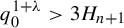
$q_0^{1+\unicode{x3bb} }>3H_{n+1}$
 . However, in view of (7.8), we have

which leads to a contradiction. This completes the proof of the lemma.
We are now prepared to prove Lemma 5.5.
Proof of Lemma 5.5
Let
$n\ge 0$
 ,
$\Omega \in \mathscr {B}^{\prime }_n$
 ,
$k\ge 1$
 . We need to prove that there is a hyperplane
$L_k(\Omega )$
 such that for any
$\Omega '\in \mathscr {B}_{n+k}$
 with
$\Omega '\subset \Omega $
 and any
$\mathbf {v}\in \mathcal {V}_{\Omega ',k}$
 , we have
$\Delta (\mathbf {v},\epsilon )\cap \Omega '\subset L_k(\Omega )^{(R^{-(n+k)}\rho _0)}$
 . We need only to consider the case that
${\Delta (\mathbf {v},\epsilon )\cap \Omega '\ne \varnothing }$
 . By Lemma 7.3, one of the following statements holds:
-
(i) there is a plane $L_k(\Omega )$
such that for any
$\Omega '\in \mathscr {B}_{n+k}$
with
$\Omega '\subset \Omega $
, if
$\mathbf {v}\in \mathcal {V}_{\Omega ',k}$
and
$\Delta (\mathbf {v},\epsilon )\cap \Omega \ne \varnothing $
, then
$L(\Omega ',\mathbf {v})=L_k(\Omega )$
; -
(ii) $k=1$
and there is
$\mathbf {v}_0=(p_0,r_0,q_0)\in \Xi $
with
$\tfrac 13H_{n+1}^{({1}/{1+\unicode{x3bb} _{\Omega }})}\leq q_0\leq 3H_{n+2}$
such that for any
$\Omega '\in \mathscr {B}_{n+1}$
with
$\Omega '\subset \Omega $
, if
$\mathbf {v}\in \mathcal {V}_{\Omega ',1}$
and
$\Delta (\mathbf {v},\epsilon )\cap \Omega \neq \varnothing $
, then
$\mathbf {v}=\mathbf {v}_0$
.











Suppose that statement (i) holds. Let us fix such a
$\Omega '$
 and denote
$\unicode{x3bb} _{\Omega '}=\unicode{x3bb} ',\;\rho _{\Omega '}=\rho '$
 . By Lemma 7.1, it suffices to show that

First, we have

Denote
$\mathbf {w}(\Omega ',\mathbf {v})=(a,b,c)$
 . If
$(x,y,z)\in \Delta _{\unicode{x3bb} '}(\mathbf {v}, 3\epsilon )\cap B_{\Omega '}$
 , then

Note that

Thus,

This means that
$I_{\Omega '}\times \{(x,y,z)\}\subset L(\Omega ',\mathbf {v})^{(R^{-(n+k)}\rho _0)}$
 . This proves (7.9).
Suppose that statement (ii) holds. Let us write
$\unicode{x3bb} _{\Omega }=\unicode{x3bb} ,\;\rho _{\Omega }=\rho $
 . Consider the hyperplane

We proceed by showing that
$\Delta (\mathbf {v}_0,\epsilon )\cap \Omega \subset L_1(\Omega )^{(R^{-n+1}\rho _0)}$
 . By Lemma 7.1, it suffices to show that

If
$(x,y,z)\in \Delta _{\unicode{x3bb} }(\mathbf {v}_0,3\epsilon )\cap B_{\Omega }$
 , then

This means that
$I_{\Omega }\times \{(x,y,z)\}\subset L_1(\Omega )^{(R^{-(n+1)\rho _0})}.$
 This proves (7.10).
Acknowledgements
Both authors would like to thank Jinpeng An and Dmitry Kleinbock for their helpful discussions and considerable suggestions. L.G. is supported by National Key R&D Program of China No. 2022YFA1007800, NSFC and Zhejiang Province 2022XHSJJ010.





