



1. Introduction
1.1. Money exchange models
The money exchange model is a type of agent-based model used to study how wealth distribution and inequality evolve through monetary exchanges between individuals. This model has been studied extensively in the field of econophysics, particularly by applying ideas from statistical physics, where the money exchange is viewed as analogous to the transfer of energy between particles in physical systems.
Consider an economy consisting of a finite number of agents. The typical process proceeds as follows.
-
(i) Initial conditions. Assign each agent a random or equal amount of money.
-
(ii) Selecting pairs of agents. Select uniformly at random a pair of agents who will exchange money.
-
(iii) Money exchange. The selected pair of agents exchange money according to specific rules.
-
(iv) Iteration. Repeat (ii) and (iii) multiple times and observe how the distribution of money in the system changes.
The primary focus of this model is to identify the limiting wealth distributions that emerge at the macroscopic level, given the microscopic rules governing the exchanges among agents. Depending on the rules of exchange, the limiting distribution is often expected to take the form of a gamma or an exponential distribution. In the field of econophysics, various studies have been conducted through numerical simulations and other methods (cf. [Reference Chakrabarti, Chakraborti, Chakravarty and Chatterjee2, Reference Greenberg and Gao10, Reference Yakovenko and Barkley Rosser26] and references therein). However, mathematically rigorous studies of these models remain relatively few.
We begin by describing several specific models. The first is the immediate exchange model proposed in [Reference Heinsalu and Patriarca11]. In this model, the wealth of each agent is represented by a real-valued variable. At each time step, two agents are randomly chosen and give a random fraction of their wealth to each other. The fraction is determined by independent uniformly distributed random variables on the interval [0, 1]. Heinsalu and Patriarca [Reference Heinsalu and Patriarca11] studied the model through numerical simulations, and later, Katriel [Reference Katriel12] analytically explored the infinite-population version. As a more realistic microscopic model that includes spatial structure in the form of local interactions representing a social network, Lanchier and Reed [Reference Lanchier and Reed16] formulated the corresponding discrete version as an interacting particle system. We briefly explain their model and result. Consider a finite connected graph
 $\mathcal{G}=(\mathcal{V}, \mathcal{E})$
. Each site
 $x\in \mathcal{V}$
corresponds to an agent, and the economy is represented by the set of agents
 $\mathcal{V}$
. The population size is given by
 $|\mathcal{V}|=N$
. The amount of money each agent holds is represented by the number of coins, where
 $M_n(x)$
represents the number of coins that agent
 $x \in \mathcal{V}$
possesses at time n. The edge set
 $\mathcal{E}$
represents a social network in which only agents connected by an edge can interact to exchange coins. At each time step, an edge
 $e=\{x, y\}\in \mathcal{E}$
is chosen uniformly at random from
 $\mathcal{E}$
. Agents x and y independently and uniformly select a random number of their coins to give to each other. Thus,
 $\{(M_n(x))_{x\in \mathcal{V}}\}_{n\geq 0}$
constitutes a time-homogeneous Markov chain. In particular, the total number of coins is conserved in this process, and we denote this total by L. Lanchier and Reed [Reference Lanchier and Reed16] proved that the stationary distribution
 $\mu_{N, L}$
for this Markov chain uniquely exists and gave the following explicit representation:
 \begin{align}\begin{split}\lim_{n\to \infty}\textrm{P}(M_n(x) = c)& = \mu_{N, L}\bigl( \{\xi\in \mathbb{Z}_+^{\mathcal{V}};\; \xi(x)= c \}\bigr) \\& =\frac{(c+1)\left(\begin{array}{c}L-c + 2N -3 \\2N-3\end{array}\right)}{\left(\begin{array}{c}L+ 2N-1 \\2N-1\end{array}\right)},\end{split}\end{align}
for every
 $x\in \mathcal{V}$
and
 $c\in \{0,1, 2, \ldots, L\}$
. The first equality is a consequence of the Markov chain convergence theorem. Then, by applying formal calculations to the right-hand side, the authors obtained the following approximation:
 \begin{equation}\lim_{n\to \infty}\textrm{P}(M_n(x) = c)\approx \frac{4c}{T^2}\textrm{e}^{-\frac{2c}{T}},\end{equation}
for large enough N and
 $T=L/N$
. In this context T represents the average number of coins per agent and is called the money temperature by analogy with the temperature in physics, and the limits
 $N\to\infty$
and
 $T=L/N \to \infty$
are respectively called the large-population limit and the large-money-temperature limit. The right-hand side of (2) is the probability density function of the gamma distribution with mean T and shape parameter 2, and this is consistent with the result predicted by [Reference Heinsalu and Patriarca11, Reference Katriel12]. As related results, [Reference Cirillo, Redig and Ruszel4, Reference van Ginkel, Redig and Sau9] examined the duality between the real-valued model and the discrete-state version in a continuous-time setting. In addition, [Reference van Ginkel, Redig and Sau9] considered the case where the exchange fraction is determined by a beta distribution.
We also present two models with different exchange rules that we address in this paper. In the uniform reshuffling model, all the coins agents x and y possess are pooled and uniformly redistributed between the two agents. Different from the immediate exchange model, the limiting distribution for this model is predicted to be an exponential distribution with mean T (cf. [Reference Dragulescu and Yakovenko6]). Lanchier and Reed [Reference Lanchier and Reed16] obtained the corresponding approximation given by
 \begin{equation}\lim_{n\to \infty}\textrm{P}(M_n(x) = c)\approx \frac{1}{T}\textrm{e}^{-\frac{c}{T}},\end{equation}
for large enough N and
 $T=L/N$
.
In the uniform saving model, agents x and y independently save a random number of their coins according to a uniform distribution. The remaining coins are then pooled and uniformly redistributed between the two agents. As for the immediate exchange model, the limiting distribution for this model is predicted to be a gamma distribution with shape parameter 2 (cf. [Reference Chakraborti and Chakrabarti3, Reference Patriarca, Chakraborti and Kaski21]), and Lanchier and Reed [Reference Lanchier and Reed16] obtained the same approximation as (2). It is worth noting that the uniform saving model can be interpreted as a combination of the above two models in the sense that it combines choosing a random number of coins like in the immediate exchange model and redistributing the coins left uniformly at random as in the uniform reshuffling model.
Lanchier and Reed [Reference Lanchier and Reed16] formulated several money exchange models as Markov chains with spatial structure, characterized their stationary distributions, and further obtained their formal approximations. Their conclusions explain the distribution of wealth in a sense, as predicted by numerical simulations and other methods. However, the approximations (
 $\approx$
) in (2) and (3) are not mathematically valid. The left-hand sides are defined only for nonnegative integers c, while the right-hand sides represent probability density functions on
 $\mathbb{R}_+$
. The derivations of the approximations (2) and (3), although merely formal calculations, seem to depend on assumptions that are not fully clarified. Specifically, in the proofs of Theorems 1, 2, and 3 in [Reference Lanchier and Reed16],
 $L+1, L+2, \ldots, L+N$
are replaced with L for sufficiently large L and N satisfying
 $N \ll L$
. On the other hand,
 $L-c+1, L-c+2, \ldots, L-c+N$
are replaced with
 $L-c$
, rather than L, even when
 $c\ll L$
. In addition,
 $c+1$
has been conveniently replaced with c. As a matter of fact, it seems unnatural to consider the approximation of
 $\mu_{N, L}( \{\xi\in \mathbb{Z}_+^{\mathcal{V}};\;\xi(x)= c \} )$
for each c since the average number of coins per agent diverges in the limit as
 $T=L/N \to \infty$
. The money exchange model describes the microscopic movement of money, however, our goal is to derive the macroscopic distribution of wealth in the limit as
 $N\to \infty$
and
 $L/N \to \infty$
. In order to do that, we should analyze the convergence of
 $\mu_{N, L}$
under appropriate scaling. Therefore, the primary objective of this paper is to provide a mathematically rigorous justification of the approximations (2) and (3), and to clearly demonstrate the convergence of the wealth distribution. Furthermore, we generalize the rules of money exchange as follows.
-
• Randomly select the number of coins to pass or save based on a probability distribution that depends on the number of coins, rather than using the uniform distribution.
-
• Allow the exchange or redistribution of coins among randomly selected groups of three or more agents, thus replacing the underlying complete graph in the original models and the underlying connected graph in [Reference Lanchier and Reed16] with the structure of a hypergraph.
These generalizations appear natural from both mathematical and economic perspectives. We note that as a generalization of the exchange rules in the immediate exchange model, [Reference Redig and Sau25] considered a broader class of models where mass is split, exchanged and merged. In [Reference Lanchier14, Reference Lanchier and Reed17, Reference Lanchier and Reed18], the authors formulated other money exchange models as Markov chains and studied their stationary distributions and formal approximations in a manner similar to (1), (2), and (3). Lanchier [Reference Lanchier15, Section 7.5.3] provides a summary of [Reference Lanchier14, Reference Lanchier and Reed16–Reference Lanchier and Reed18] as well as other mathematical papers in econophysics. In addition, the mixing time has recently been studied for the binomial splitting model and the symmetric beta-binomial splitting model, which are variations of the uniform reshuffling model (cf. [Reference Pymar and Rivera23, Reference Quattropani and Sau24]).
Before introducing our models and results we set out some useful notation. In the following,
 $\mathbb{Z}_+=\{0, 1, 2, \ldots \}$
denotes the set of nonnegative integers and
 $\mathbb{N}=\{1, 2, 3, \ldots \}$
denotes the set of positive integers. Here
 $\lfloor a \rfloor$
denotes the integer part of
 $a>0$
and we set
 $a \vee b\; :\!= \max\{a, b\}$
and
 $a \wedge b\; :\!= \min\{a, b\}$
for
 $a, b \in \mathbb{R}$
. For a finite set
 $A \subset \mathbb{N}$
,
 $|A|$
denotes its cardinality. For two sequences of positive numbers
 $\{a_n\}$
and
 $\{b_n\}$
,
 $a_n\sim b_n$
means that
 $\lim_{n\to \infty}\frac{a_n}{b_n}=1$
. A function f on
 $\mathbb{R}^{\mathbb{Z}}$
is called local if it depends only on finitely many coordinates. For a probability measure
 $\mu$
,
 $\mathbb{E}^\mu[\, \cdot\, ]$
denotes the expectation with respect to
 $\mu$
. A hypergraph is a pair
 $\mathcal{H}= (\mathcal{V}, \mathcal{E})$
where
 $\mathcal{V}$
is a set of vertices (or nodes), and
 $\mathcal{E}$
is a set of hyperedges, where each hyperedge is a subset of
 $\mathcal{V}$
that can contain any number of vertices. Unlike in a standard graph, where edges connect only two vertices, hyperedges in a hypergraph can connect two or more vertices at once.
1.2. Model description and results
Let us state our model precisely. We adopt the standard notation commonly used in the study of interacting particle systems. For
 $A \subset \mathbb{N}$
and
 $L \in \mathbb{N}$
, we define the configuration space
 \begin{equation*}\Omega(A, L)=\left\{\xi = \{\xi(x)\}_{x\in A} \in \mathbb{Z}_+^A;\;\sum_{x\in A}\xi(x) =L\right\}.\end{equation*}
When
 $A=\Lambda_N\; :\!= \{1, 2, \ldots, N\}$
,
 $\Omega(A, L)$
is denoted by
 $\Omega_N(L)$
. Consider now an economy populated by many agents. Each site
 $x\in \Lambda_N$
corresponds to an agent and we assume that the economy can be represented by the set of agents
 $\Lambda_N$
. N corresponds to the population size. For each
 $\xi \in \Omega_N(L)$
, we interpret
 $\xi(x)$
,
 $x\in \Lambda_N$
, not as the number of particles, but as the number of coins held by agent x.
 $\rho$
denotes a probability distribution on
 $\mathcal{D}_N= \{ A\subset \Lambda_N;\; |A|\geq 2\}$
, namely
 $\rho(A)\geq 0$
for every
 $A \subset \Lambda_N$
with
 $|A|\geq 2$
and
 $\sum_{A\in \mathcal{D}_N}\rho(A)=1$
. This represents the distribution that determines which agents handle the money exchange at each time step. We also take a nonnegative function
 $g ( {\not}\!\equiv 0)$
defined on
 $\mathbb{Z}_+$
. We now introduce three money exchange models.
Immediate exchange model. Let
 $\{X_n\}_{n \geq 0}$
be a time-homogeneous Markov chain on the state space
 $\Omega_N(L)$
. For given
 $X_n=\xi \in \Omega_N(L)$
, the configuration
 $X_{n+1}$
is determined from the following rule.
-
(i) Choose a hyperedge
 $A\in \mathcal{D}_N$
according to the distribution
$\rho$
.
-
(ii) For given
$\xi$
, let
$\{c(x)\}_{x\in A}$
be independent random variables whose distributions are given by (4)for
\begin{equation}\textrm{P}(c(x)=k)= \frac{1}{G(\xi(x))}g(k),\quad k\in \{ 0, 1, 2, \ldots, \xi(x)\},\end{equation}
$x\in A$
where we set
$G(k) = \sum_{j=0}^k g(j)$
,
$k\in \mathbb{Z}_+$
.
-
(iii) Choose a permutation
$\sigma \in \mathcal{S}_A$
uniformly at random, namely with probability
$\frac{1}{|\mathcal{S}_A|}=\frac{1}{|A|!}$
where
$\mathcal{S}_A$
denotes the set of all permutations of A. -
(iv) For given
$\xi$
and realizations A,
$\{c(x)\}_{x\in A}$
and
$\sigma$
, define
$X_{n+1}$
by
\begin{equation*}X_{n+1}(z) =\begin{cases}\xi(z) -c(z) + c(\sigma^{-1}(z)) & \text{if } z \in A, \\\xi(z) & \text{if } z \notin A. \\\end{cases}\end{equation*}


This dynamics can be interpreted as follows. At each time step, a money exchange occurs between agents in a randomly chosen set A. Here c(x) represents the number of coins that agent x transfers, which is determined by a probability distribution dependent on the weight function g and the number of coins,
 $\xi(x)$
, that agent x possesses. According to a randomly chosen permutation
 $\sigma\in \mathcal{S}_A$
, each agent
 $x \in A$
passes c(x) coins to agent
 $\sigma(x)\in A$
; see Figure 1. In this process, the total number of coins remains conserved. It is worth noting that the model studied in [Reference Lanchier and Reed16] corresponds to the case where g is a constant function and
 $\rho$
is the uniform distribution on an edge set of
 $\Lambda_N$
. In this case, the distribution (4) matches the uniform distribution on
 $\{0, 1, 2, \ldots, \xi(x)\}$
and the money exchange occurs between two agents connected by an edge in
 $\Lambda_N$
. To be more precise, since the permutation
 $\sigma\in \mathcal{S}_A$
can include the identity permutation, our model can be viewed as the lazy version of their model in this case.
Immediate exchange dynamics. In this case, the hyperedge is
 $A = \{2,4,5,8\}$
and the random permutation is
 $\sigma(2)=5$
,
 $\sigma(4)=2$
,
 $\sigma(5)=8$
, and
 $\sigma(8)=4$
.

Uniform reshuffling model. Let
 $\{Y_n\}_{n \geq 0}$
be a time-homogeneous Markov chain on the state space
 $\Omega_N(L)$
. For given
 $Y_n=\xi$
, the configuration
 $Y_{n+1}$
is determined from the following rule.
-
(i) Choose a hyperedge
$A\in \mathcal{D}_N$
according to the distribution
$\rho$
. -
(ii) For given
$\xi$
and A, choose a configuration
$d =\{d(x)\}_{x\in A}\in \Omega(A, S_A(\xi))$
uniformly at random, namely with probability
$\frac{1}{|\Omega(A, S_A(\xi))|}$
where we set
$ S_A(\xi)= \sum_{x\in A}\xi(x)$
for
$\{\xi(x)\}_{x\in A}$
. -
(iii) For given
$\xi$
and realizations A and
$\{d(x)\}_{x\in A}$
, define
$Y_{n+1}$
by
\begin{equation*}Y_{n+1}(z) =\begin{cases}d(z) & \text{if } z \in A, \\\xi(z) & \text{if } z \notin A. \\\end{cases}\end{equation*}


This is an extension of the model studied in [Reference Lanchier and Reed16], which considered the dynamics between two agents, to the dynamics on a hypergraph. At each time step, a redistribution of coins occurs among the agents in a randomly chosen set A. Specifically, the configuration restricted to A is replaced by a configuration chosen uniformly at random among all the configurations with the same number of coins on the set A.
Random saving model. Let
 $\{Z_n\}_{n \geq 0}$
be a time-homogeneous Markov chain on the state space
 $\Omega_N(L)$
. For given
 $Z_n=\xi$
, the configuration
 $Z_{n+1}$
is determined from the following rule.
-
(i) Choose a hyperedge
$A\in \mathcal{D}_N$
according to the distribution
$\rho$
. -
(ii) For given
$\xi$
, let
$\{c(x)\}_{x\in A}$
be independent random variables whose distributions are given by for
\begin{equation*}\textrm{P}(c(x)=k)= \frac{1}{G(\xi(x))}g(k),\quad k\in \{ 0, 1, 2, \ldots, \xi(x)\},\end{equation*}
$x\in A$
.
-
(iii) For given
$\xi$
and
$c=\{c(x)\}_{x\in A}$
, choose a configuration
$d =\{d(x)\}_{x\in A}\in \Omega(A, S_A(\xi)-S_A(c))$
uniformly at random, namely with probability
$\frac{1}{|\Omega(A, S_A(\xi)-S_A(c))|}$
. -
(iv) For given
$\xi$
and realizations A,
$\{c(x)\}_{x\in A}$
and
$\{d(x)\}_{x\in A}$
, define
$Z_{n+1}$
by
\begin{equation*}Z_{n+1}(z) =\begin{cases}c(z) + d(z) & \text{if } z \in A, \\\xi(z) & \text{if } z \notin A. \\\end{cases}\end{equation*}


Note that in contrast to the immediate exchange model, the random variable c(x) represents how many coins the agent x saves. The random saving model can be interpreted as a combination of the immediate exchange model and the uniform reshuffling model where the agents in the hyperedge choose a random number of coins (as in the immediate exchange model) to save rather to give, and then all the coins left are uniformly redistributed among the agents (like in the uniform reshuffling model). Similarly to the immediate exchange model, [Reference Lanchier and Reed16] studied the case where g is a constant function and
 $\rho$
is the uniform distribution on an edge set. In that model, c(x) is drawn from the uniform distribution on
 $\{0, 1, 2, \ldots, \xi(x)\}$
, and it is referred to as the uniform saving model. Since our model considers a more general distribution for c(x), we refer to it as the random saving model. As a special case, when the weight function g is defined by
 $g(k)=\delta_0(k)$
for
 $k\in \mathbb{Z}_+$
, each agent saves no money. When a money exchange occurs within set A, all coins held by the agents in A are pooled and redistributed. This dynamics corresponds to the uniform reshuffling model, and in particular, the uniform reshuffling model can be seen as a special case of the random saving model.
As the first result, we characterize the stationary distributions of these Markov chains.
Proposition 1.1. Let
 $N, L \in \mathbb{N}$
be fixed. We assume that the hypergraph
 $(\Lambda_N, \mathcal{D}_{N, \rho})$
is connected, where the hyperedge set
 $\mathcal{D}_{N, \rho}$
is defined by
 $\mathcal{D}_{N, \rho} = \{A\subset \Lambda_N;\; |A|\geq2,\rho(A)>0\}$
.
-
(i) Assume that the weight function
$g\,:\,\mathbb{Z}_+ \to [0, \infty)$
satisfies
$g(0)>0$
and
$g(1)>0$
. Then there is a unique stationary distribution
$\mu_{N, L}$
for
$\{X_n\}_{n \geq 0}$
and it is given by (5)where
\begin{equation}\mu_{N, L}(\xi) = \frac{1}{Z_{N, L}}\prod_{x\in \Lambda_N}\!\! G(\xi(x)), \quad\xi \in \Omega_N(L),\end{equation}
$G(k) = \sum_{j=0}^k g(j),\ k \in \mathbb{Z}_+$
, and
$Z_{N, L}= \sum_{\xi \in \Omega_N(L)}\prod_{x\in \Lambda_N} G(\xi(x))$
is the normalization factor. In particular, for every
$\eta \in \Omega_N(L)$
,
$x\in \Lambda_N$
, and
$k \in \{0, 1, 2, \ldots, L\}$
, we have that where
\begin{align*}\lim_{n \to \infty} \textrm{P}_{\eta}\bigl( X_n(x) = k \bigr)= \mu_{N, L}\bigl( \xi(x) =k \bigr) =\frac{Z_{N-1, L-k}\, G(k)}{Z_{N, L}},\end{align*}
$\textrm{P}_\eta$
represents the law of
$\{X_n\}_{n\geq 0}$
with the initial condition
$X_0=\eta$
.
-
(ii) Assume that the weight function
$g\,:\,\mathbb{Z}_+ \to [0, \infty)$
satisfies
$g(0)>0$
. Then the exact same statement as (i) applies to
$\{Z_n\}_{n \geq 0}$
instead of
$\{X_n\}_{n \geq 0}$
. In particular, for the uniform reshuffling model
$\{Y_n\}_{n\geq 0}$
, there is a unique stationary distribution
$\pi_{N, L}$
and it is given by the uniform distribution on
$\Omega_N(L)$
, namely,
\begin{equation*}\pi_{N, L}(\xi) = \frac{1}{|\Omega_{N}(L)|}, \quad\xi \in \Omega_N(L).\end{equation*}


By this proposition we can see that both the immediate exchange model and the random saving model have the same stationary distribution under the conditions
 $g(0)>0$
and
 $g(1)>0$
. In addition, the choice of
 $\rho$
does not affect the stationary distribution. Lanchier and Reed [Reference Lanchier and Reed16] proved that, for dynamics on a graph, the stationary distribution does not depend on the topology of the underlying connected graph. The present result generalizes this finding to the setting of dynamics on a hypergraph.
Remark 1.1. The condition
 $g(0)>0$
is always needed to make the measure (5) well-defined. Furthermore, the conditions
 $g(0)>0$
and
 $g(1)>0$
for the immediate exchange model, as well as the condition
 $g(0)>0$
for the random saving model, ensure that these Markov chains are irreducible and aperiodic.
Remark 1.2. Consider the case where the weight function g is a constant function
 $g \equiv \gamma>0$
. Then
 $G(k)= \gamma(k+1)$
,
 $k\in \mathbb{Z}_+$
, and the constant
 $\gamma$
is canceled by the normalization factor in the definition of
 $\mu_{N, L}$
. Therefore, we can take G as
 $G(k)= k+1$
,
 $k\in \mathbb{Z}_+$
, in (5) and in this case the above result matches that of [Reference Lanchier and Reed16]. Lanchier and Reed [Reference Lanchier and Reed16] also gave the explicit representation for
 $Z_{N, L}$
when
 $g\equiv 1$
and obtained (1).
Remark 1.3. For the random saving model we can change the role of random variable c(x) to represent the number of coins to offer instead of the number of coins to save. Namely, we modify (iii) and (iv) in the definition of the random saving model as follows.
-
(iii)′ For given
$\xi$
and
$c=\{c(x)\}_{x\in A}$
, choose a configuration
$d =\{d(x)\}_{x\in A}\in \Omega(A, S_A(c))$
uniformly at random, namely with probability
$\frac{1}{|\Omega(A, S_A(c))|}$
. -
(iv)′ For given
$\xi$
and realizations A,
$\{c(x)\}_{x\in A}$
and
$\{d(x)\}_{x\in A}$
, define
$Z_{n+1}$
by
\begin{equation*}Z_{n+1}(z) =\begin{cases}\xi(z)-c(z) + d(z) & \text{if } z \in A, \\\xi(z) & \text{if } z \notin A. \\\end{cases}\end{equation*}


By symmetry, the exact same proof for Proposition 1.1 below works well in this setting and the same result holds for this modified model.
We are now in a position to state the main result of this paper. To justify the limit
 $N\to \infty$
and
 $L/N \to \infty$
, we assume that the total number of coins
 $L=L_N$
satisfies
 $\lim_{N\to\infty}\frac{L_N}{Na_N}=T$
for some
 $T>0$
and divergent sequence
 $\{a_N\}_{N\geq 1}$
. Then we can prove that the law of the scaled field
 $\bigl\{ \frac{1}{a_N}\eta(x)\bigr\}_{x\in \Lambda_N}$
under
 $\mu_{N, L}$
or
 $\pi_{N, L}$
converges to the independent and identically distributed (i.i.d.) product of probability distributions on
 $\mathbb{R}_+$
. Its marginal distribution depends on the asymptotic behavior of the weight function g.
Theorem 1.1. Let
 $\{L_N \}_{N\geq 1}$
be a sequence of positive integers that satisfies
 $\lim_{N\to\infty}\frac{L_N}{N a_N}=T$
for some positive constant
 $T>0$
and a sequence
 $\{a_N\}_{N\geq 1}$
which satisfies
 $\lim_{N\to \infty}a_N=\infty$
. Assume that
 $g(0)>0$
, and that there exist
 $\alpha\in \mathbb{R}$
and
 $c_\alpha \in (0, \infty)$
such that
 $\lim_{k\to \infty}\frac{g(k)}{k^\alpha} =c_\alpha$
. Then, for every bounded continuous local function
 $f\,:\,\mathbb{R}^A \to \mathbb{R}$
, we have that
 \begin{align*}\lim_{N\to \infty}\mathbb{E}^{\mu_{N, L_N }} \Bigl[ f\biggl(\frac{\cdot}{a_N} \biggr)\Bigr]=\mathbb{E}^{\overline{\mu}_{\alpha, T}^A}\bigl[f(\, \cdot\, )\bigr],\end{align*}
where A is a finite subset of
 $\mathbb{N}$
and
 $\overline{\mu}_{\alpha, T}^A$
denotes the product probability measure on
 $\mathbb{R}_+^A$
whose one-site marginal distribution on
 $\mathbb{R}_+$
is given by
 \begin{align}\mu_{\alpha, T}(dr) =\begin{cases}\displaystyle\frac{1}{\Gamma(\alpha+2)} \left(\frac{\alpha+2}{T}\right)^{\alpha +2} r^{\alpha +1} \textrm{e}^{-\frac{\alpha+2}{T}r}\,dr & \text{if } \alpha>-1, \\\displaystyle\frac{1}{T} \textrm{e}^{-\frac{1}{T}r}\,dr& \text{if } \alpha \leq -1,\end{cases}\end{align}
in which
 $\Gamma(\beta)= \int_0^\infty r^{\beta-1}\textrm{e}^{-r}\,dr$
is the Gamma function with parameter
 $\beta>0$
.
In addition, if
 $g\,:\, \mathbb{Z}_+\to [0, \infty)$
satisfies
 $g(0)>0$
and
 $\sum_{j\geq 0} g(j) <\infty$
, then the same conclusion as in the case
 $\alpha\leq -1$
above holds. In particular, for every bounded continuous local function
 $f\,:\,\mathbb{R}^A \to \mathbb{R}$
,
 \begin{align*}\lim_{N\to \infty}\mathbb{E}^{\pi_{N, L_N }} \left[ f\left(\frac{\cdot}{a_N} \right)\right]=\mathbb{E}^{{\overline{\pi}}_{T}^A}\bigl[f(\, \cdot\, )\bigr],\end{align*}
where A is a finite subset of
 $\mathbb{N}$
and
 $\overline{\pi}_{T}^A$
denotes the product probability measure on
 $\mathbb{R}_+^A$
whose one-site marginal distribution on
 $\mathbb{R}_+$
is given by
 $\pi_{T}(dr) =\frac{1}{T} \textrm{e}^{-\frac{1}{T}r}\,dr$
.
As an easy consequence of Proposition 1.1 and Theorem 1.1 we obtain the following result.
Corollary 1.1. Let
 $\{X_n^{(N)}\}_{n\geq 0}$
,
 $\{Y_n^{(N)}\}_{n\geq 0}$
, and
 $\{Z_n^{(N)}\}_{n\geq 0}$
denote the immediate exchange model, the uniform reshuffling model and the random saving model on the state space
 $\Omega_{N}(L_N)$
, respectively. Under the same conditions as in Proposition 1.1 and Theorem 1.1, we have
 \begin{align*}\lim_{N\to \infty}\lim_{n\to \infty}\mathbb{E}_{\eta} \Biggl[ \frac{1}{N}\biggm|\!\biggl\{x\in \Lambda_N;\;\frac{1}{a_N} {X_n^{(N)} (x)} \in (b, c) \biggr\}\!\biggm|\Biggr]= \mu_{\alpha, T}((b, c)),\end{align*}
 \begin{align*}\lim_{N\to \infty}\lim_{n\to \infty}\mathbb{E}_{\eta} \Biggl[ \frac{1}{N}\biggm|\!\biggl\{x\in \Lambda_N;\;\frac{1}{a_N} {Y_n^{(N)} (x)} \in (b, c) \biggr\}\!\biggm|\Biggr]= \pi_{T}((b, c))\end{align*}
and
 \begin{align*}\lim_{N\to \infty}\lim_{n\to \infty}\mathbb{E}_{\eta} \Biggl[ \frac{1}{N}\biggm|\!\biggl\{x\in \Lambda_N;\;\frac{1}{a_N} {Z_n^{(N)} (x)} \in (b, c) \biggr\}\!\biggm|\Biggr]= \mu_{\alpha, T}((b, c)),\end{align*}
for every
 $\eta \in \Omega_N(L_N)$
and every
 $0 \leq b < c \leq \infty$
, where
 $\mathbb{E}_{\eta}[\ \cdot \ ]$
denotes the expectation with respect to the law of the Markov chain with the initial condition
 $\eta$
.
We note that it is natural to consider the scaling of the process by a factor of
 $\frac{1}{a_N}$
. This is because, under the condition on
 $L_N$
, we have
 \[\frac{1}{N}\sum_{x\in \Lambda_N} \left(\frac{1}{a_N}X_n^{(N)} (x)\right) = \frac{L_N}{Na_N}= T(1+o(1)) \quad \text{as }N\to \infty,\]
which means that the asymptotic average number of coins per agent for the scaled process is given by T. This value corresponds to the money temperature in our model. Corollary 1.1 provides a precise formulation and generalization of earlier studies in the physics literature, which were based on numerical simulations and heuristic arguments. As time approaches infinity, and in the large-population and large-money-temperature limit, the asymptotic wealth distribution (i.e. the proportion of agents holding a specific number of coins) converges to either a gamma distribution or an exponential distribution for both the immediate exchange model and the random saving model, while it converges to an exponential distribution for the uniform reshuffling model. The parameters of the gamma distribution depend on the asymptotic behavior of the weight function g. When
 $\alpha>-1$
, the limiting wealth distribution is given by a gamma distribution with mean T and shape parameter
 $\alpha +2$
. When
 $\alpha \leq -1$
, the limiting wealth distribution is given by an exponential distribution with mean T, and this does not depend on the parameter
 $\alpha$
. In particular, if g is a constant function then
 $\alpha=0$
and the limiting distribution is a gamma distribution with mean T and shape parameter 2, which corresponds to (2). In addition, when
 $g(k)=(k+1)^{\alpha}$
,
 $k\in \mathbb{Z}_+$
, the above results are consistent with numerical simulations (see Figures 2 and 3).
Simulation results for a single realization of the immediate exchange model and the random saving model with
 $g(k)=(k+1)^{\alpha}$
, where
 $\alpha = 1, 3$
. The number of agents is
 $N=10^4$
and the total number of coins is
 $L=10^6$
, namely the average number of coins per agent is 100. The initial condition is set to a constant configuration
 $X_0 \equiv 100$
or
 $Z_0 \equiv 100$
. Here
 $\rho$
is distributed uniformly over the set of hyperedges consisting of all three-element subsets of distinct vertices in
 $\Lambda_N$
, and in the immediate exchange model, one of the three-element permutations is selected with probability
 $\frac{1}{6}$
. The gray histograms represent the wealth distribution (i.e. the proportion of agents holding a specific number of coins after
 $n=10^5$
updates). The dotted line is the graph of the probability density function of the gamma distribution
 $f_{a, b}(r)=\frac{1}{\Gamma(a)b^{a}} r^{ a-1}\textrm{e}^{-\frac{1}{b}r}$
, with shape parameter
 $a=\alpha+2$
and scale parameter
 $b= \frac{100}{\alpha+2}$
.

Figure 2 Long description
The image contains four graphs comparing wealth distribution models. Each graph shows the probability density of the number of coins held by agents after 100,000 updates. The top-left graph represents the immediate exchange model with g(r) = r + 1, showing a wealth distribution that closely follows a gamma distribution with shape parameter 3 and scale parameter 100/3. The top-right graph represents the random saving model with the same g(r) function, displaying a similar wealth distribution. The bottom-left graph shows the immediate exchange model with g(r) = (r + 1)^3, where the wealth distribution aligns with a gamma distribution with shape parameter 5 and scale parameter 100/5. The bottom-right graph depicts the random saving model with the same g(r) function, presenting a comparable wealth distribution. All graphs illustrate how different exchange rules and parameters influence the wealth distribution among agents.
Simulation results for a single realization of the immediate exchange model and the random saving model with
 $g(k)=(k+1)^{\alpha}$
, where
 $\alpha = -1, -2$
. The settings of the simulations are the same as in Figure 2. The dotted line is the graph of the probability density function of the exponential distribution
 $f_{\lambda}(r)= {\lambda}\textrm{e}^{-\lambda r}$
with the parameter
 $\lambda=\frac{1}{100}$
. When the weight function g decays rapidly in the immediate exchange model, the probability of each agent exchanging only a small number of coins at a time increases, leading to a longer convergence time to reach a steady state. The simulation result for the case
 $g(k)=(k+1)^{-2}$
reflects this and
 $n=10^5$
updates are not sufficient for convergence (middle left). However, after
 $n=10^6$
updates, the histograms approach the limiting probability density function (lower left). In addition, the result for the case
 $N=10^3$
and
 $n=10^6$
indicates that we need to take a large population N (and, hence, a large L) for convergence (lower right).

Figure 3 Long description
The image contains six histograms showing wealth distribution in different models with varying parameters and time steps. Each histogram compares the wealth distribution to an exponential distribution with a parameter of 0.01. The top row shows the immediate exchange model with g(r) = (r + 1)^(-1) and N = 10^4, n = 10^5, and the random saving model with g(r) = (r + 1)^(-1) and N = 10^4, n = 10^5. The middle row shows the immediate exchange model with g(r) = (r + 1)^(-2) and N = 10^4, n = 10^5, and the random saving model with g(r) = (r + 1)^(-2) and N = 10^4, n = 10^5. The bottom row shows the immediate exchange model with g(r) = (r + 1)^(-2) and N = 10^4, n = 10^6, and the immediate exchange model with g(r) = (r + 1)^(-2) and N = 10^3, n = 10^6. The histograms illustrate how the wealth distribution changes with different parameters and time steps, showing convergence to the exponential distribution in some cases.
Remark 1.4. The limiting distribution (6) for the case
 $\alpha \leq -1$
can be interpreted as follows: If the weight function g decays rapidly in the random saving model, the probability that each agent saves a large number of coins becomes very small. Moreover, since we are considering the scaled process
 $\left\{\frac{1}{a_N}Z_n^{(N)}\right\}_{n\geq 0}$
, we can assume that each agent offers nearly all the coins they have in each money exchange. Consequently, similarly to the uniform reshuffling model, the limiting distribution becomes an exponential distribution with mean T. In the immediate exchange model, when the weight function g decays rapidly, the probability that each agent exchanges a large number of coins also becomes very small. For the scaled process, this situation can be regarded as similar to the one-coin model, where one agent gives only one coin to another agent at a time. In the one-coin model, the limiting distribution is expected to be exponential (cf. [Reference Dragulescu and Yakovenko6, Reference Lanchier14]) and the result above aligns with this. Furthermore, a mathematically rigorous justification of the result for the one-coin model can be achieved by formulating and proving it in the same manner as demonstrated in this paper.
1.3. Discussion
Here we examine some further extensions of the model whose stationary distributions are not explicitly known.
Nonuniform permutation. In the immediate exchange model, given a hyperedge
 $A\in \mathcal{D}_N$
, a permutation
 $\sigma \in \mathcal{S}_A$
is chosen uniformly at random. One may also consider choosing it according to a general probability distribution
 $Q_A$
on
 $\mathcal{S}_A$
. If
 $Q_A$
possesses good symmetry properties for every
 $A\in \mathcal{D}_N$
, then the proof of Proposition 1.1 applies, and the stationary distribution is given by (5); see Remark 2.1 following the proof of Proposition 1.1. However, in the general case, the situation remains unclear.
Individual allocation. In the random saving model, after the agents within a hyperedge determine how many coins to save, the remaining coins are pooled and then redistributed uniformly at random among them. Alternatively, one could consider a setting in which each agent individually distributes their remaining coins to the other members of the selected hyperedge. Namely, we modify (iii) and (iv) in the definition of the random saving model as follows.
-
(iii)′′ For given
$\xi$
and
$c=\{c(x)\}_{x\in A}$
, for each
$x\in A$
, choose a configuration
$d^x =\{ d^x(y) \}_{y\in A \setminus \{ x \}}\in \Omega(A\setminus \{x\}, \xi(x)-c(x))$
uniformly at random, namely with probability
$\frac{1}{|\Omega(A\setminus \{x\}, \xi(x)-c(x))|}$
. -
(iv)′′ For given
$\xi$
and realizations A,
$\{c(x)\}_{x\in A}$
and
$\{\{d^x(y)\}_{y\in A\setminus \{x\}};\; x\in A\}$
, define
$Z_{n+1}$
by
\begin{equation*}Z_{n+1}(z) =\begin{cases}c(z) + \sum\limits_{x \in A \setminus \{z\}}d^x(z) & \text{if } z \in A, \\\xi(z) & \text{if } z \notin A. \\\end{cases}\end{equation*}


In this dynamics, each agent
 $x\in A$
distributes
 $\xi(x)-c(x)$
coins by giving
 $d^x(y)$
coins to each other agent
 $y \in A\setminus \{x\}$
. As a result, at time
 $n+1$
, the number of coins held by each agent equals the sum of the coins they saved and those received from other agents. This model can also be viewed as an extension of the immediate exchange model studied in [Reference Lanchier and Reed16], since, when
 $\rho$
is supported on the set of edges of
 $\Lambda_N$
, the above redistribution rule coincides with the immediate exchange model on a graph. The proof of Proposition 1.1 relies on the fact that the number of coins received can be represented by a single variable. When the received amount is instead expressed as a sum of multiple variables, the situation becomes considerably more complicated, and the explicit form of the stationary distribution remains unknown.
In the rest of the paper we provide the proofs of Proposition 1.1 and Theorem 1.1 in Sections 2 and 3, respectively. We give some comments about the strategy of the proof. The proof of Proposition 1.1 is standard. It is not difficult to see that our models are irreducible and aperiodic Markov chains on the finite state space
 $\Omega_N(L)$
. All we have to do is to characterize the unique stationary distribution, which is achieved by carefully verifying the detailed balance condition. Namely, we demonstrate that our models are reversible Markov chains, and the reversible distributions for
 $\{X_n\}_{n\geq 0}$
and
 $\{Z_n\}_{n\geq 0}$
are given by (5). With respect to the proof of Theorem 1.1, the convergence of the marginal distribution of
 $\mu_{N, L}$
is closely related to the equivalence of ensembles (cf. [Reference Friedli and Velenik8, Reference Kipnis and Landim13]). The sequence
 $\{G(k)\}_{k\in \mathbb{Z}_+}$
is neither a probability distribution nor summable over k. However, multiplying G(k) by the exponential factor
 $s^k$
,
 $s\in [0, 1)$
, ensures the convergence of
 $\sum_{k\in \mathbb{Z}_+}s^kG(k)$
under the assumption on g. The stationary distribution (5) can then be interpreted as the microcanonical distribution of an i.i.d. product, where the one-site marginal distribution is of exponential type and proportional to G. Instead of the usual condition
 $\frac{1}{N}\sum_{x\in \Lambda_N}\eta(x) \to m \in (0, \infty)$
as
 $N\to \infty$
, we consider the condition
 $\frac{1}{Na_N}\sum_{x\in \Lambda_N}\eta(x) \to T \in (0, \infty)$
and investigate the convergence of the law of the scaled field
 $\frac{1}{a_N}\eta$
under the corresponding microcanonical distribution. We adapt the proof of the equivalence of ensembles from [Reference Kipnis and Landim13, Appendix 2] to this unusual setting. In particular, the local limit theorem for a triangular array of random variables plays an important role in the argument.
Throughout the paper C, C ′, and C ″ represent positive constants that do not depend on the size of the system N, but may depend on other parameters. These constants in various estimates may change from place to place in the paper.
2. Proof of Proposition 1.1
In this section we prove Proposition 1.1. Under the condition that the hypergraph
 $(\Lambda_N, \mathcal{D}_{N, \rho})$
is connected, we have that for every
 $x, y\in \Lambda_N$
there exists a sequence
 $\{A_k\}_{0 \leq k \leq l}\subset \mathcal{D}_{N, \rho}$
such that
 $x\in A_0$
,
 $y\in A_l$
, and
 $A_{k} \cap A_{k+1}\ne \emptyset$
for every
 $0 \leq k \leq l-1$
. Combining this fact with the assumption
 $g(0)>0$
and
 $g(1)>0$
, it is easy to see that the following assertions hold.
-
• For every
$\xi, \eta\in \Omega_N(L)$
there exists
$m=m(\xi, \eta)\geq 0$
such that
$\textrm{P}(X_{m} = \eta | X_0=\xi) >0$
. -
•
$\textrm{P}(X_{n+1} = \eta | X_n=\eta) >0$
for every
$\eta \in \Omega_N(L)$
and
$n\geq 0$
.


The same statements also hold for
 $\{Z_n\}_{n\geq 0}$
under the condition
 $g(0)>0$
. Namely,
 $\{X_n\}_{n \geq 0}$
and
 $\{Z_n\}_{n \geq 0}$
are irreducible and aperiodic Markov chains on the finite state space
 $\Omega_N(L)$
. Note that for the immediate exchange model,
 $g(0)>0$
implies that all the agents keep all their coins with positive probability, which leads to aperiodicity (the second condition above). If in addition
 $g(1)>0$
, with positive probability, exactly one agent gives exactly one coin while the other agents give no coins, which allows us to move one coin from a given vertex to another given vertex in a finite number of time steps and leads to irreducibility (the first condition above). Similarly, the condition
 $g(0)>0$
ensures irreducibility and aperiodicity for the random saving model. Then the stationary distribution of
 $\{X_n\}_{n \geq 0}\ (\{Z_n\}_{n \geq 0})$
uniquely exists and the law of
 $X_n\ (Z_n)$
converges to it regardless of the initial configuration of coins in the limit
 $n \to \infty$
by the Markov chain convergence theorem. Therefore, all we have to show is that the measure
 $\mu_{N, L}$
given by (5) is the stationary distribution for both of
 $\{X_n\}_{n \geq 0}$
and
 $\{Z_n\}_{n \geq 0}$
. Actually, by verifying the detailed balance condition,
 \begin{equation}\mu_{N , L}(\xi) \textrm{P}(X_{n+1} = \eta | X_n=\xi)=\mu_{N , L}(\eta) \textrm{P}(X_{n+1} = \xi | X_n=\eta) \quad\text{for every } \xi, \eta\in \Omega_N(L)\end{equation}
and
 \begin{equation}\mu_{N , L}(\xi) \textrm{P}(Z_{n+1} = \eta | Z_n=\xi)=\mu_{N , L}(\eta) \textrm{P}(Z_{n+1} = \xi | Z_n=\eta) \quad\text{for every } \xi, \eta\in \Omega_N(L),\end{equation}
we prove that (5) is the reversible distribution for both of
 $\{X_n\}_{n \geq 0}$
and
 $\{Z_n\}_{n \geq 0}$
. In addition, the result for the uniform reshuffling model
 $\{Y_n\}_{n\geq 0}$
follows from taking the weight function g as
 $g(k)=\delta_0(k)$
for
 $k\in \mathbb{Z}_+$
in the random saving model.
Proof for the immediate exchange model. Take arbitrary
 $\xi, \eta \in \Omega_N(L)$
and set
 $A_0=A_0(\xi, \eta)\; :\!=\{x \in \Lambda_N;\, \xi(x) \ne \eta(x)\}$
. We have that
 \begin{align*}& \textrm{P}(X_{n+1} = \eta | X_n=\xi) \\& =\sum_{{\substack{A\in \mathcal{D}_N \\ A\supset A_0}}}\rho(A) \sum_{\sigma \in \mathcal{S}_A}\frac{1}{|\mathcal{S}_A|}\textrm{P}\bigl(\eta(z)= \xi(z)-c(z) + c(\sigma^{-1}(z)) \text{ for every }z\in A \bigm|\! \xi \bigr),\end{align*}
where
 $\textrm{P}(\ \cdot \ | \xi )$
denotes the law of
 $\{c(x)\}_{}$
in the dynamics (ii) given the configuration
 $\xi$
. If
 $\rho(A)=0$
for every
 $A\in \mathcal{D}_N$
so that
 $A\supset A_0$
, then the right-hand side is equal to 0. For a finite set A, we label its elements as
 $A=\{x_1, x_2, \ldots, x_{|A|}\}$
. Then
 \begin{align*}& \textrm{P}\bigl(\eta(z)= \xi(z)-c(z) + c(\sigma^{-1}(z)) \text{ for every }z\in A \bigm|\! \xi \bigr) \\& =\sum_{t_1=0}^{\xi(x_1)}\sum_{t_2=0}^{\xi(x_2)}\cdots\sum_{t_{|A|}=0}^{\xi(x_{|A|})}\prod_{i=1}^{|A|} \frac{g(t_i)}{G(\xi(x_i))} \cdot{\bf{1}}\bigl( \eta(x_i)= \xi(x_i)-t_i + t_{\sigma^{-1}(i)}\text{ for every } 1 \leq i \leq |A|\bigr) \\& =\sum_{t_1=0}^{\xi(x_1)}\sum_{t_2=0}^{\xi(x_2)}\cdots\sum_{t_{|A|}=0}^{\xi(x_{|A|})}\prod_{i=1}^{|A|} \Biggl\{\frac{g(t_i)}{G(\xi(x_i))}{\bf{1}}\bigl( \eta(x_i)= \xi(x_i)-t_i + t_{\sigma^{-1}(i)}\bigr)\Biggr\},\end{align*}
where for each
 $\sigma \in \mathcal{S}_A$
and
 $1\leq i\leq |A|$
, we identify
 $\sigma^{-1}(i)$
with the label
 $1\leq k \leq |A|$
which satisfies
 $x_k= \sigma^{-1}(x_i)$
. Therefore,
 \begin{align}\begin{split}&\Biggl\{ \prod_{x \in \Lambda_N} G(\xi(x)) \Biggr\} \cdot\textrm{P}(X_{n+1} = \eta | X_n=\xi) \\& =\sum_{{\substack{A\in \mathcal{D}_N \\ A\supset A_0}}}\Biggl[\prod_{x \in \Lambda_N\setminus A}\!\!G(\xi(x)) \cdot\frac{\rho(A)}{|\mathcal{S}_A|} \\& \qquad \qquad\times\sum_{\sigma \in \mathcal{S}_A}\sum_{t_1=0}^{\xi(x_1)}\sum_{t_2=0}^{\xi(x_2)}\cdots\sum_{t_{|A|}=0}^{\xi(x_{|A|})}\prod_{i=1}^{|A|} \Bigl\{{g(t_i)}{\bf{1}}\bigl( \eta(x_i)= \xi(x_i)-t_i + t_{\sigma^{-1}(i)}\bigr)\Bigr\}\Biggr] \\& =\sum_{{\substack{A\in \mathcal{D}_N \\ A\supset A_0}}}\Biggl[\prod_{x \in \Lambda_N\setminus A}\!\!\Biggl\{\frac{G(\xi(x))+G(\eta(x))}{2}\Biggr\} \cdot\frac{\rho(A)}{|\mathcal{S}_A|} \\& \qquad \qquad\times\sum_{\sigma \in \mathcal{S}_A}\sum_{t_1=0}^{\xi(x_1)}\sum_{t_2=0}^{\xi(x_2)}\cdots\sum_{t_{|A|}=0}^{\xi(x_{|A|})}\prod_{i=1}^{|A|} \Bigl\{{g(t_i)}{\bf{1}}\bigl( \eta(x_i)= \xi(x_i)-t_i + t_{\sigma^{-1}(i)}\bigr)\Bigr\}\Biggr],\end{split}\end{align}
where the last equality follows from
 $\xi = \eta$
on
 $\Lambda_N\setminus A_0$
. The symmetry of this expression with respect to
 $\xi$
and
 $\eta$
implies the detailed balance condition (7). For
 $A\subset \Lambda_N$
and
 $\sigma \in \mathcal{S}_A$
, we set
 \begin{equation*}h_A(\sigma, \xi, \eta)\; :\!=\sum_{t_1=0}^{\xi(x_1)}\sum_{t_2=0}^{\xi(x_2)}\cdots\sum_{t_{|A|}=0}^{\xi(x_{|A|})}\prod_{i=1}^{|A|} \Bigl\{{g(t_i)}{\bf{1}}\bigl( \eta(x_i)= \xi(x_i)-t_i + t_{\sigma^{-1}(i)}\bigr)\Bigr\}.\end{equation*}
To show that (9) is symmetric with respect to
 $\xi$
and
 $\eta$
, it is sufficient to show that
 $\sum_{\sigma \in \mathcal{S}_A}h_A(\sigma, \xi, \eta)$
is symmetric with respect to
 $\xi$
and
 $\eta$
for every
 $A\in \mathcal{D}_N$
so that
 $A\supset A_0$
. Now, each permutation
 $\sigma \in\mathcal{S}_A$
can be decomposed as the product of cyclic permutations and the summand in
 $h_A(\sigma, \xi, \eta)$
is given by a product form. Accordingly, the following two statements are sufficient for the symmetry of
 $\sum_{\sigma \in \mathcal{S}_A}h_A(\sigma, \xi, \eta)$
.
-
• When
$|A|=2$
,
$h_A(\sigma, \xi, \eta)$
is symmetric with respect to
$\{\xi(x)\}_{x \in A}$
and
$\{\eta(x)\}_{x \in A}$
for every
$\sigma \in\mathcal{S}_A$
. -
• When
$|A|\geq 3$
,
$h_A(\sigma, \xi, \eta)+ h_A(\sigma^{-1}, \xi, \eta)$
is symmetric with respect to
$\{\xi(x)\}_{x \in A}$
and
$\{\eta(x)\}_{x \in A}$
for every cyclic permutation
$\sigma \in\mathcal{S}_A$
.


These can be reformulated as follows.
Lemma 2.1. Let
 $g\,:\, \mathbb{Z}_+ \to [0, \infty)$
and
 $a= \{a_i\}_{i=1}^n, b= \{b_i\}_{i=1}^n \in\mathbb{Z}_+^n$
be two sequences of nonnegative integers which satisfy
 $\sum_{i=1}^n a_i =\sum_{i=1}^n b_i$
.
-
(i) Let
$n=2$
and define where we identify
\begin{align*}S=S(a, b)\; :\!=\sum_{t_1=0}^{a_1}\sum_{t_2=0}^{a_2}\prod_{i=1}^{2} \{{g(t_i)}{\bf{1}}( t_i - t_{i+1} = a_i-b_i ) \},\end{align*}
$t_3$
as
$t_1$
. Then S is symmetric with respect to a and b.
-
(ii) Let
$n\geq 3$
and define where we identify
\begin{align*}S=S_+(a, b) + S_-(a, b)& \; :\!=\sum_{t_1=0}^{a_1}\sum_{t_2=0}^{a_2}\cdots \sum_{t_n=0}^{a_n}\prod_{i=1}^{n} \{{g(t_i)}{\bf{1}}( t_i - t_{i+1} = a_i-b_i )\} \\& \qquad+\sum_{t_1=0}^{a_1}\sum_{t_2=0}^{a_2}\cdots \sum_{t_n=0}^{a_n}\prod_{i=1}^{n} \{{g(t_i)}{\bf{1}}( t_i - t_{i-1} = a_i-b_i )\},\end{align*}
$t_{n+1}$
as
$t_1$
and
$t_0$
as
$t_n$
. Then S is symmetric with respect to a and b.


Proof.
-
(i) Under the condition
$a_1+a_2= b_1+b_2$
, we have This is symmetric with respect to a and b because
\begin{align*}S(a, b)& =\sum_{t_1=0}^{a_1}\sum_{t_2=0}^{a_2}g(t_1)g(t_1-a_1+b_1){\bf{1}}( t_{2} = t_1 -a_1+b_1 ) \\& =\sum_{t_1=0}^{a_1}g(t_1)g(t_1-a_1+b_1){\bf{1}}( 0 \leq t_1 -a_1+b_1 \leq a_2 ) \\& =\sum_{t_1=0 \vee (a_1-b_1)}^{a_1\wedge (a_1+a_2 -b_1)}g(t_1)g(t_1-a_1+b_1) \\& =\sum_{t_1=0 \vee (a_1-b_1)}^{a_1\wedge b_2}g(t_1)g(t_1-a_1+b_1) \\& =\sum_{t_1= a_1 \vee b_1}^{(a_1+b_1) \wedge (b_1+b_2)}g(t_1-b_1 )g(t_1-a_1).\end{align*}
$b_1+b_2= \frac{1}{2}(a_1+a_2+b_1+b_2)$
.
-
(ii) We compute that
Similarly,
\begin{align*}& S_+(a, b) \\& =\sum_{t_1 \geq 0}\sum_{t_2 \geq 0}\cdots \sum_{t_n\geq 0}\Biggl[\prod_{i=1}^{n} \{{g(t_i)}{\bf{1}}( t_i - t_{i+1} = a_i-b_i )\}\prod_{i=1}^{n}\{{\bf{1}}( t_i \leq a_i) {\bf{1}}( t_{i+1} \leq b_i )\}\Biggr] \\& =\sum_{t_1 \geq 0}\sum_{t_2 \geq 0}\cdots \sum_{t_n\geq 0}\prod_{i=1}^{n}{g(t_i)}\prod_{i=1}^{n} \{{\bf{1}}( t_i - t_{i+1} = a_i-b_i ){\bf{1}}( t_i \leq a_i\wedge b_{i-1} )\}.\end{align*}
where the second equality follows from rewriting the variable
\begin{align*}& S_-(a, b) \\& =\sum_{t_1 \geq 0}\sum_{t_2 \geq 0}\cdots \sum_{t_n\geq 0}\prod_{i=1}^{n}{g(t_i)}\prod_{i=1}^{n} \{{\bf{1}}( t_i - t_{i-1} = a_i-b_i ){\bf{1}}( t_i \leq a_i\wedge b_{i+1} )\} \\& =\sum_{t_1 \geq 0}\sum_{t_2 \geq 0}\cdots \sum_{t_n\geq 0}\prod_{i=1}^{n}{g(t_i)}\prod_{i=1}^{n} \{{\bf{1}}( t_{i+1} - t_{i} = a_i-b_i ){\bf{1}}( t_{i+1} \leq a_i\wedge b_{i+1} )\} \\& =\sum_{t_1 \geq 0}\sum_{t_2 \geq 0}\cdots \sum_{t_n\geq 0}\prod_{i=1}^{n}{g(t_i)}\prod_{i=1}^{n} \{{\bf{1}}( t_{i} - t_{i+1} = b_i-a_i ){\bf{1}}( t_{i} \leq a_{i-1} \wedge b_{i} )\}\\& =S_+(b, a),\end{align*}
$t_i$
as
$t_{i+1}$
,
$1\leq i \leq n$
. Therefore,
$S_+(a, b)+S_-(a, b)$
is symmetric with respect to a and b.


Remark 2.1. Consider the case where, for each
 $A\in \mathcal{D}_N$
, a permutation
 $\sigma \in \mathcal{S}_A$
is chosen according to a general probability distribution
 $Q_A$
on
 $\mathcal{S}_A$
, instead of the uniform distribution. Following the argument above, if we can show that
 $\sum_{\sigma \in \mathcal{S}_A}Q_A(\sigma)h_A(\sigma, \xi, \eta)$
is symmetric with respect to
 $\xi$
and
 $\eta$
for every
 $A \in \mathcal{D}_N$
so that
 $A\supset A_0$
, then the stationary distribution is given by (5), just as in the case where
 $\sigma$
is chosen uniformly at random. As a sufficient condition, suppose that, for every
 $A\in \mathcal{D}_N$
and every collection of disjoint cyclic permutations that compose a permutation on
 $A$
, the permutations generated by these cycles and their inverses are assigned equal probabilities under
 $Q_A$
. Then the symmetry of
 $\sum_{\sigma \in \mathcal{S}_A}Q_A(\sigma)h_A(\sigma, \xi, \eta)$
holds. As an illustrative example, consider a permutation
 $\widetilde{\sigma}=\sigma_1\sigma_2\in \mathcal{S}_A$
where
 $\sigma_1$
and
 $\sigma_2$
are two disjoint cyclic permutations. Assume that all permutations on
 $A$
formed as products of
 $\sigma_1$
,
 $\sigma_2$
and their inverses occur with equal probability
 $Q_A(\widetilde{\sigma})$
. Then their total contribution to the sum
 $\sum_{\sigma \in \mathcal{S}_A}Q_A(\sigma)h_A(\sigma, \xi, \eta)$
is given by
 $$Q_A(\widetilde{\sigma})\bigl\{h_A(\sigma_1\sigma_2, \xi, \eta)+h_A(\sigma_1\sigma_2^{-1}, \xi, \eta)+h_A(\sigma_1^{-1}\sigma_2, \xi, \eta)+h_A(\sigma_1^{-1}\sigma_2^{-1}, \xi, \eta)\bigr\}.$$
The symmetry of the expression
 $$h_A(\sigma_1\sigma_2, \xi, \eta)+h_A(\sigma_1\sigma_2^{-1}, \xi, \eta)+h_A(\sigma_1^{-1}\sigma_2, \xi, \eta)+h_A(\sigma_1^{-1}\sigma_2^{-1}, \xi, \eta)$$
with respect to
 $\xi$
and
 $\eta$
then follows from the preceding proof.
Proof for the random saving model. We use similar notation to the proof for the immediate exchange model. Take arbitrary
 $\xi, \eta \in \Omega_N(L)$
. We have
 \begin{align*}&\textrm{P}(Z_{n+1} = \eta | Z_n=\xi) \\& =\sum_{{\substack{A\in \mathcal{D}_N \\ A\supset A_0}}}\rho(A)\textrm{P}\bigl(\eta(z)= c(z) + d(z) \text{ for every }z\in A \bigm| \xi \bigr) \\& =\sum_{{\substack{A\in \mathcal{D}_N \\ A\supset A_0}}}\rho(A)\sum_{t_1=0}^{\xi(x_1)}\sum_{t_2=0}^{\xi(x_2)}\cdots\sum_{t_{|A|}=0}^{\xi(x_{|A|})}\Biggl[\prod_{i=1}^{|A|} \frac{g(t_i)}{G(\xi(x_i))}\sum\limits_{\zeta \in\Omega(A, S_A(\xi)-S_A(t))}\frac{1}{|\Omega(A, S_A(\xi)-S_A(t))|} \\& \qquad \qquad \qquad \qquad \qquad \qquad \qquad \qquad\times{\bf{1}}\bigl( \eta(x_i)= t_i + \zeta(x_i)\text{ for every } 1 \leq i \leq |A|\bigr) \Biggr] \\& =\sum_{{\substack{A\in \mathcal{D}_N \\ A\supset A_0}}}\rho(A)\sum_{t_1=0}^{\xi(x_1)\wedge \eta(x_1)}\sum_{t_2=0}^{\xi(x_2)\wedge \eta(x_2)}\cdots\sum_{t_{|A|}=0}^{\xi(x_{|A|})\wedge \eta(x_{|A|})}\Biggl[\prod_{i=1}^{|A|} \frac{g(t_i)}{G(\xi(x_i))} \times \\& \quad\sum\limits_{\zeta \in\Omega(A, S_A(\xi)-S_A(t))}\frac{1}{|\Omega(A, S_A(\xi)-S_A(t))|}{\bf{1}}\bigl( \eta(x_i)= t_i + \zeta(x_i)\text{ for every } 1 \leq i \leq |A|\bigr)\Biggr],\end{align*}
where
 $S_A(t)=\sum_{i=1}^{|A|}t_i$
for
 $t=\{t_i\}_{i=1}^{|A|}$
. We have
 $S_A(\xi)=S_A(\eta)$
for
 $A\supset A_0$
. In addition, for given
 $t=\{t_i\}_{i=1}^{|A|}$
so that
 $0 \leq t_i \leq \xi(x_i) \wedge \eta(x_i)$
for every
 $1\leq i \leq |A|$
, there exists a unique
 $\zeta \in \Omega(A, S_A(\xi)-S_A(t))$
which satisfies
 $\eta(x_i)= t_i + \zeta(x_i)$
for every
 $1 \leq i \leq |A|$
. Therefore,
 \begin{align*}&\Biggl\{ \prod_{x \in \Lambda_N} G(\xi(x))\Biggr\} \cdot\textrm{P}(Z_{n+1} = \eta | Z_n=\xi) \\& \quad =\sum_{{\substack{A\in \mathcal{D}_N \\ A\supset A_0}}}\Biggl[\prod_{x \in \Lambda_N\setminus A} \Biggl\{\frac{G(\xi(x))+G(\eta(x))}{2}\Biggr\} \cdot{\rho(A)}\\ & \qquad \times\sum_{t_1=0}^{\xi(x_1)\wedge \eta(x_1)}\sum_{t_2=0}^{\xi(x_2)\wedge \eta(x_2)}\cdots\sum_{t_{|A|}=0}^{\xi(x_{|A|})\wedge \eta(x_{|A|})}\prod_{i=1}^{|A|}{g(t_i)}\cdot\frac{1}{|\Omega(A, \frac{S_A(\xi)+S_A(\eta)}{2}-S_A(t))|}\Biggr].\end{align*}
Since the expression is symmetric with respect to
 $\xi$
and
 $\eta$
, we obtain (8).
If we define g as
 $g(k)=\delta_0(k)$
,
 $k\in \mathbb{Z}_+$
, then
 $G\equiv 1$
and the above argument yields that
 $\textrm{P}(Z_{n+1} = \eta | Z_n=\xi)$
is symmetric with respect to
 $\xi$
and
 $\eta$
. Therefore, the uniform reshuffling model is doubly stochastic and its unique stationary distribution is given by the uniform distribution on
 $\Omega_{N}(L)$
. Actually, this matches when
 $G\equiv 1$
is set in (5).
3. Proof of Theorem 1.1
For the proof of Theorem 1.1, we adapt the proof of the equivalence of ensembles for the i.i.d. product measure (cf. [Reference Kipnis and Landim13, Appendix 2]). In the following we assume that
 $g(0)>0$
and there exist
 $\alpha\in \mathbb{R}$
and
 $c_\alpha \in (0, \infty)$
such that
 $\lim_{k\to \infty}\frac{g(k)}{k^\alpha} =c_\alpha$
. We set out the required notation. Define
 $G(k)=\sum_{j=0}^k g(j)$
,
 $k\in \mathbb{Z}_+$
, and
 $Q_n(s)=\sum_{k\geq 0} k^n s^k G(k)$
,
 $n \in \mathbb{Z}_+$
. By the assumption on g, we have the following asymptotics for G(k) as
 $k\to \infty$
:
 \begin{equation}G(k) \sim\begin{cases}\displaystyle\frac{c_\alpha}{\alpha +1}k^{\alpha +1} &\text{if } \alpha > -1, \\{c_\alpha}{\log k} &\text{if } \alpha = -1, \\C_0 &\text{if } \alpha < -1, \\\end{cases}\end{equation}
where
 $C_0=C_0(g)>0$
is a constant which depends on g. In particular, the radius of convergence of
 $Q_n(s)$
is 1 and we have that
 $\lim_{s\uparrow 1}Q_n(s) = \infty$
for every
 $n\in \mathbb{Z}_+$
and
 $\alpha \in \mathbb{R}$
. We define the exponential family of distributions
 $\{\nu_s(\, \cdot\, ) ;\, s \in [0, 1)\}$
on
 $\mathbb{Z}_+$
by
 $\nu_s (k) = \frac{s^k G(k)}{Q_0(s)}$
,
 $k \in \mathbb{Z}_+$
. It is easy to see that
 $\mathbb{E}^{\nu_s}[\eta(0)] = \frac{Q_1(s)}{Q_0(s)}$
is continuous, increasing in s and diverges to infinity as
 $s\uparrow 1$
. Hence, for every
 $K>0$
there exists a unique
 ${s}^*={s}^*(K) \in (0, 1)$
such that
 $\mathbb{E}^{\nu_{s^*}}[\eta(0)] = K$
. To examine the asymptotic behavior of
 $s^*(K)$
as
 $K \to \infty$
, we use a Tauberian theorem of the following form (cf. [Reference Bingham, Goldie and Teugels1, Corollary 1.7.3]).
Theorem 3.1. Let
 $\{a_k\}_{k\geq 0}$
be a sequence of nonnegative numbers and assume that
 $A(s)=\sum_{k=0}^\infty a_k s^k$
converges for
 $s\in [0, 1)$
and
 $\{a_k\}_{k\geq 0}$
is monotone. Then the following assertions are equivalent:
-
•
$A(s) \sim \Gamma(\beta +1) (1-s)^{-\beta} h(\frac{1}{1-s})$
as
$s \uparrow 1$
for
$\beta >0$
and slowly varying function h; -
•
$a_k \sim \beta k^{\beta-1} h(k)$
as
$k\to \infty$
for
$\beta >0$
and slowly varying function h.


By this theorem and (10), the following asymptotics holds in the limit as
 $s\uparrow 1$
:
 \begin{equation}Q_n(s) \sim\begin{cases}\displaystyle\frac{c_\alpha \Gamma(n+\alpha + 2)}{\alpha +1}(1-s)^{-(\alpha +n+2)} &\text{if } \alpha > -1, \\[2pt]{c_\alpha \Gamma( n+1)}(1-s)^{-(n+1)} \log \displaystyle\frac{1}{1-s}&\text{if } \alpha = -1, \\[2pt]{C_0 \Gamma( n+1)}(1-s)^{-(n+1)} &\text{if } \alpha < -1,\end{cases}\end{equation}
where we used the relation
 $\Gamma (\beta +1) =\beta \Gamma(\beta)$
for every
 $\beta>0$
. Therefore,
 \begin{equation*}\mathbb{E}^{\nu_s}[\eta(0)] = \frac{Q_1(s)}{Q_0(s)} \sim\begin{cases}\displaystyle\frac{\alpha + 2}{1-s} &\text{if } \alpha > -1, \\[2pt]\displaystyle\frac{1}{1-s} &\text{if } \alpha \leq -1, \\\end{cases}\end{equation*}
and this yields that
 \begin{equation}s^*(K) =\begin{cases}1- \displaystyle\frac{\alpha + 2}{K}(1+o(1)) &\text{if } \alpha > -1, \\[2pt]1- \displaystyle\frac{1}{K}(1+o(1)) &\text{if } \alpha \leq -1, \\\end{cases}\end{equation}
as
 $K\to \infty$
. By these asymptotics we also have
 \begin{align}\textrm{Var}_{\nu_{s^*(K)}}(\eta (0))&=\displaystyle\frac{Q_2(s^*(K))}{Q_0(s^*(K))} -K^2\\&=\begin{cases}\displaystyle\frac{1}{\alpha + 2}{K^2}(1+o(1)) &\text{if } \alpha > -1, \\[3pt]{K^2}(1+o(1)) &\text{if } \alpha \leq -1, \\ \end{cases} \nonumber \end{align}
as
 $K\to \infty$
.
Next, for each
 $s \in [0, 1)$
and
 $B \subset \mathbb{N}$
, let
 $\overline{\nu}_s^B$
be the product measure on
 $\mathbb{Z}_+^B$
whose one-site marginal distribution equals
 $\nu_s$
.
 $\overline{\nu}_s^{B}\bigl(\, \cdot\, \bigm| \Omega(B, L) \bigr)$
denotes the conditioned probability of
 $\overline{\nu}_s^B$
on the event that the total number of coins on B equals to L. Then we have the following key identity for (5):
 \begin{equation*}\mu_{N, L}(\, \cdot\,) =\overline{\nu}_s^{\Lambda_N}\bigl(\, \cdot\, \bigm| \Omega_N(L) \bigr).\end{equation*}
Note that the right-hand side does not depend on the choice of the parameter s. Let
 $f\,:\,\mathbb{R}^A \to \mathbb{R}$
be a bounded continuous local function where A is a finite subset of
 $\mathbb{N}$
. For every
 $N\in \mathbb{N}$
such that
 $\Lambda_N \supset A$
, we have
 \begin{align}& \mathbb{E}^{\mu_{N, L}}\biggl[ f\left(\frac{\cdot}{a_N} \right)\biggr] \nonumber \\& =\sum\limits_{\eta\in \mathbb{Z}_+^A}f\left( \frac{\eta}{a_N} \right)\overline{\nu}_s^{\Lambda_N}\left( \xi_A = \eta \bigm| \sum\limits_{x\in \Lambda_N}\xi(x)= L \right) \nonumber\\& =\sum\limits_{\eta\in \mathbb{Z}_+^A}f\left( \frac{\eta}{a_N} \right)\overline{\nu}_s^{A}(\eta)+\sum\limits_{\eta\in \mathbb{Z}_+^A}f\left( \frac{\eta}{a_N} \right)\left\{\frac{\overline{\nu}_s^{\Lambda_N \setminus A}\left( \sum\limits_{x\in \Lambda_N\setminus A}\xi(x)= L -S_A(\eta)\right)}{\overline{\nu}_s^{\Lambda_N }\left( \sum\limits_{x\in \Lambda_N}\xi(x)= L \right)}-1\right\} \overline{\nu}_s^{A}(\eta)\nonumber\\& =\!:\; I_1 +I_2,\end{align}
where
 $\xi_A$
denotes the configurations
 $\xi$
restricted to the set A. Now, we set
 $L=L_N$
where
 $\{L_N \}_{N\geq 1}$
is a sequence of positive integers that satisfies
 $\lim_{N\to\infty}\frac{L_N}{N a_N}=T$
for some constant
 $T>0$
and divergent sequence
 $\{a_N\}_{N\geq 1}$
. We also take s on the right-hand side of (14) as
 $s_N^*\; :\!=s^*(\frac{L_N}{N})$
. For this choice of s we show that
 $I_1 \to \int_{\mathbb{R}_+^A} f(r)\overline{\mu}_{\alpha, T}^A(dr)$
and
 $I_2 \to 0$
as
 $N\to \infty$
.
For the proof of the convergence of
 $I_1$
, we assume that f is a function of one variable for notational simplicity. The general case can be proven in a similar manner since
 $\overline{\nu}_s^A$
is a product measure with the same marginal distribution. First, we consider the case
 $\alpha>-1$
. Let
 $R>0$
. By (10) and (11),
 \begin{align*}I_1& =\sum\limits_{k \geq 0}f\bigg( \frac{k}{a_N} \bigg) \frac{1}{Q_0(s_N^*)} (s_N^*)^k G(k) \\[3pt]& =\frac{1}{\Gamma(\alpha +2)}(1-s_N^*)\sum\limits_{k = 0}^{\lfloor R a_N \rfloor}f\bigg( \frac{k}{a_N} \bigg) (s_N^*)^k\bigl((1-s_N^*)k \bigr)^{\alpha+1} \\[3pt]& \qquad \qquad \qquad+\frac{1}{\Gamma(\alpha +2)}(1-s_N^*)\sum\limits_{k = \lfloor R a_N \rfloor +1}^\infty f\bigg( \frac{k}{a_N} \bigg) (s_N^*)^k\bigl((1-s_N^*)k \bigr)^{\alpha+1}+o(1) \\[3pt]& =\!:\; I_{3}+I_4+ o(1),\end{align*}
as
 $N\to \infty$
. We note that since
 $Q_0(s_N^*) \to \infty$
in the limit
 $N\to \infty$
, a finite sum in
 $I_1$
is negligible and we can replace G with the right-hand side of (10) with an error of o(1). Then, by (12) and the condition on
 $L_N$
,
 \begin{align*}I_3& =\frac{1}{\Gamma(\alpha +2)}\frac{\alpha+2}{T}\frac{1}{a_N}\sum\limits_{k = 0}^{\lfloor R a_N \rfloor}f\bigg( \frac{k}{a_N} \bigg)\Bigg\{\bigg(1-\frac{\alpha+2}{T}\frac{1}{a_N}\bigg)^{a_N}\Bigg\}^{\frac{k}{a_N}}\bigg(\frac{\alpha+2}{T}\frac{k}{a_N}\bigg)^{\alpha+1}+o(1) \\[3pt]&\to\frac{1}{\Gamma(\alpha+2)} \bigg(\frac{\alpha+2}{T}\bigg)^{\alpha +2} \int_0^R f(r) \textrm{e}^{-\frac{\alpha+2}{T}r}r^{\alpha +1}\,dr,\end{align*}
as
 $N\to \infty$
where the convergence follows from the definition of the Riemann integral. By taking the limit
 $R\to \infty$
, the right-hand side converges to
 $\int_0^\infty f(r) \mu_{\alpha, T}(dr)$
. For
 $I_4$
, we have
 \begin{align*}|I_4|& \leq\frac{1}{\Gamma(\alpha +2)}\frac{\alpha+2}{T}\frac{1}{a_N}\sum\limits_{k =\lfloor R a_N \rfloor +1}^{\infty}\biggm| f\bigg( \frac{k}{a_N} \bigg)\!\!\biggm|\biggl(1-\frac{\alpha+2}{T}\frac{1}{a_N}\biggr)^{k}\biggl(\frac{\alpha+2}{T}\frac{k}{a_N}\biggr)^{\alpha+1}+o(1) \\[3pt]& \leq C \frac{1}{a_N}\sum\limits_{k =\lfloor R a_N \rfloor +1}^{\infty}\textrm{e}^{-\frac{\alpha+2}{T}\frac{k}{a_N}}\biggl(\frac{k}{a_N}\biggr)^{\alpha+1}+o(1) \\[3pt]&\leq C'\sum\limits_{j =\lfloor R \rfloor}^{\infty}\textrm{e}^{-\frac{\alpha+2}{T}j}j^{\alpha+1}+o(1),\end{align*}
for every N large enough where C, C
′ are positive constants independent of N. By taking the limits
 $N\to \infty$
and
 $R\to\infty$
, we obtain
 $I_4\to 0$
.
Second, we consider the case
 $\alpha=-1$
. By (10) and (11) again,
 \begin{align*}I_1& =\frac{1-s_N^*}{-\log (1-s_N^*)}\sum\limits_{k = 0}^{\lfloor R a_N \rfloor}f\biggl( \frac{k}{a_N} \biggr) (s_N^*)^k \log k \\[3pt]& \qquad \qquad+\frac{1-s_N^*}{-\log (1-s_N^*)}\sum\limits_{k = \lfloor R a_N \rfloor +1}^\infty f\biggl( \frac{k}{a_N} \biggr) (s_N^*)^k \log k+o(1) \\[3pt]& =\!:\; I'_{3}+I'_4+ o(1),\end{align*}
as
 $N\to \infty$
. We have
 ${-\log (1-s_N^*)}=(1+o(1))\log a_N$
, and this yields that
 \begin{align*}I'_3& =\frac{1}{T a_N \log a_N}\sum\limits_{k = 0}^{\lfloor R a_N \rfloor}f\biggl( \frac{k}{a_N} \biggr)\Biggl\{\biggl(1-\frac{1}{T a_N}\biggr)^{a_N}\Biggr\}^{\frac{k}{a_N}}{\log k}+o(1) \\[3pt]& =\frac{1}{T a_N}\sum\limits_{k = 0}^{\lfloor R a_N \rfloor}f\biggl( \frac{k}{a_N} \biggr)\Biggl\{\biggl(1-\frac{1}{T a_N}\biggr)^{a_N}\Biggr\}^{\frac{k}{a_N}} \\[3pt]& \qquad +\frac{1}{T \log a_N}\frac{1}{a_N}\sum\limits_{k = 0}^{\lfloor R a_N \rfloor}f\biggl( \frac{k}{a_N} \biggr)\Biggl\{\biggl(1-\frac{1}{T a_N}\biggr)^{a_N}\Biggr\}^{\frac{k}{a_N}}\log \biggl(\frac{k}{a_N}\biggr)+o(1).\end{align*}
In the limits
 $N\to \infty$
and
 $R\to \infty $
, the first term of the right-hand side converges to
 $\frac{1}{T}\int_0^\infty f(r)\textrm{e}^{-\frac{r}{T}}\,dr$
and the second term vanishes due to the extra factor
 $\frac{1}{\log a_N}$
.
 $I'_4$
goes to 0 in the same way as
 $I_4$
. The case
 $\alpha<-1$
also follows from a similar argument.
Next, for the convergence of
 $I_2$
, we use the following local limit theorem.
Theorem 3.2. Let
 $\{b_N\}_{N \geq 1}$
be a sequence of positive numbers which satisfies
 $\lim_{N\to \infty}b_N=\infty$
and set
 $s_N^*\; :\!= s^*(b_N)$
. For each
 $N\in \mathbb{N}$
,
 $\{X_j^{(N)}\}_{j\in \Lambda_N}$
denotes a family of i.i.d.
 $\mathbb{Z}_+$
-valued random variables with common distribution
 $\nu_{s_N^*}$
. Then, for every finite set
 $B\subset \mathbb{N}$
,
 \begin{align}\lim\limits_{N\to \infty}\sup\limits_{L \geq 0} \left|\!\sqrt{\sigma_N^2(N-|B|)}\textrm{P} \left(\sum_{j \in \Lambda_N \setminus B} X_j^{(N)} =L \right) -\frac{1}{\sqrt{2\pi}}\exp\Biggl\{-\frac{( L-(N-|B|)b_N)^2}{ 2 \sigma_N^2(N-|B|)}\Biggr\}\!\right| =0,\end{align}
where
 $\sigma_N^2 = \textrm{Var}(X_1^{(N)})$
.
The proof of this theorem is given later. By applying this theorem for
 $L=L_N$
and
 $b_N=\frac{L_N}{N}$
, we have
 \begin{align*}&\frac{\overline{\nu}_{s_N^*}^{\Lambda_N \setminus A}\left( \sum\limits_{x\in \Lambda_N\setminus A}\xi(x)= L_N -S_A(\eta)\right)}{\overline{\nu}_{s_N^*}^{\Lambda_N }\left( \sum\limits_{x\in \Lambda_N}\xi(x)= L_N \right)} \\[4pt]& \qquad \qquad=\frac{\sqrt{N}}{\sqrt{N-|A|}}\frac{\exp\left\{-\frac{(L_N-S_A(\eta) -(N-|A|)\frac{L_N}{N})^2}{{2\sigma^2_N}{(N-|A|)}}\right\} + o(1)}{1 + o(1)},\end{align*}
as
 $N\to \infty$
for every
 $\eta \in \mathbb{Z}_+^A$
. Note that the o(1) terms do not depend on
 $\eta$
. Set
 $D_A(k) = \{0, 1, \ldots, k\}^A$
,
 $k\in \mathbb{Z}_+$
. Then the above asymptotics and (13) yield that
 \begin{align*}\lambda_{N, R} \; :\!=\sup\limits_{\eta \in D_A(\lfloor Ra_N \rfloor)}\left| \!\frac{\overline{\nu}_{s_N^*}^{\Lambda_N \setminus A}\left( \sum\limits_{x\in \Lambda_N\setminus A}\xi(x)= L_N -S_A(\eta)\right)}{\overline{\nu}_{s_N^*}^{\Lambda_N }\left( \sum\limits_{x\in \Lambda_N}\xi(x)= L_N \right)} -1\! \right|\to 0\end{align*}
as
 $N\to \infty$
for every
 $R>0$
, and
 \begin{align*}\sup_{N\geq 1}\sup\limits_{\eta \in \mathbb{Z}_+^A}\left|\!\frac{\overline{\nu}_{s_N^*}^{\Lambda_N \setminus A}\left( \sum\limits_{x\in \Lambda_N\setminus A}\xi(x)= L_N -S_A(\eta)\right)}{\overline{\nu}_{s_N^*}^{\Lambda_N }\left( \sum\limits_{x\in \Lambda_N}\xi(x)= L_N \right)}-1\!\right|\,\leq C''\end{align*}
for some constant
 $C''>0$
. Therefore,
 \begin{align*}|I_2|& \leq\sum\limits_{\eta \in D_A(\lfloor Ra_N \rfloor)}\biggm|\! f\biggl( \frac{\eta}{a_N} \biggr) \!\biggm|\left|\!\frac{\overline{\nu}_{s_N^*}^{\Lambda_N \setminus A}\left( \sum\limits_{x\in \Lambda_N\setminus A}\xi(x)= L_N -S_A(\eta)\right)}{\overline{\nu}_{s_N^*}^{\Lambda_N }\left( \sum\limits_{x\in \Lambda_N}\xi(x)= L_N \right)}-1 \! \right| \overline{\nu}_{s_N^*}^{A}(\eta) \\[3pt]& \qquad \quad +\sum\limits_{\eta\in\mathbb{Z}_+^A \setminus D_A(\lfloor Ra_N \rfloor)}\biggm|\! f\biggl( \frac{\eta}{a_N} \biggr) \!\biggm|\left|\!\frac{\overline{\nu}_{s_N^*}^{\Lambda_N \setminus A}\left( \sum\limits_{x\in \Lambda_N\setminus A}\xi(x)= L_N -S_A(\eta)\right)}{\overline{\nu}_{s_N^*}^{\Lambda_N }\left( \sum\limits_{x\in \Lambda_N}\xi(x)= L_N \right)}-1\! \right| \overline{\nu}_{s_N^*}^{A}(\eta) \\[3pt]& \leq\| f\|_{\infty}\lambda_{N, R} +C''\sum\limits_{\eta\in\mathbb{Z}_+^A \setminus D_A(\lfloor Ra_N \rfloor )}\left| f\left( \frac{\eta}{a_N} \right) \!\right|\overline{\nu}_{s_N^*}^{A}(\eta).\end{align*}
The first term on the right-hand side goes to 0 as
 $N\to \infty$
for every
 $R>0$
, and the second term goes to 0 as
 $N\to\infty$
and
 $R\to \infty$
by a similar computation to the estimate of
 $I_4$
above. Hence, we obtain
 $I_2 \to 0$
and this completes the proof.
If we assume the condition
 $g(0)>0$
and
 $\sum_{j\geq 0} g(j) <\infty$
for
 $g\,:\,\mathbb{Z}_+\to [0, \infty)$
instead, then the proof for the case
 $\alpha<-1$
above can be applied as it is.
Remark 3.1. If
 $( L-(N-|B|)b_N)^2 \gg { 2 \sigma_N^2(N-|B|)}$
in (15) then the exponential term converges to 0, rendering the local limit theorem ineffective. For this reason, the local limit theorem in the form of Theorem 3.2 was insufficient to prove the equivalence of ensembles in general settings, and a more refined version such as the Edgeworth expansion of at least the second order was necessary (cf. the proofs of Corollaries 1.4 and 1.7 in [Reference Kipnis and Landim13, Appendix 2]). On the other hand, such an expansion is not necessary and Theorem 3.2 is sufficient in our case. Because we divided the summation
 $\sum_{\eta \in \mathbb{Z}_+^A}$
of
 $I_2$
into
 $\sum_{\eta \in D_A(\lfloor Ra_N \rfloor)}$
and
 $\sum_{\eta \in\mathbb{Z}_+^A \setminus D_A(\lfloor Ra_N \rfloor)}$
, the estimate for the latter part was reduced to the estimate of
 $\overline{\nu}_{s_N^*}^{A}(\mathbb{Z}_+^A \setminus D_A(\lfloor Ra_N \rfloor))$
which can be managed because we know the explicit form of
 ${\nu}_{s_N^*}$
.
Proof of Theorem 3.2. First of all, we note that Theorem 3.2 corresponds to the local limit theorem for a triangular array of random variables since
 $\nu_{s_N^*}$
depends on the number of random variables N. Combining this with the fact that
 $s_N^*\; :\!= s^*(b_N) \to 1$
as
 $N\to \infty$
, we cannot apply Theorem 1.3 or 1.5 directly in [Reference Kipnis and Landim13, Appendix 2] which studied the refined version of the local limit theorem for the i.i.d. random variables with common distribution
 $\nu_s$
,
 $s\in (0, 1)$
. In addition, the known criteria of the local limit theorem for a triangular array of integer-valued random variables (e.g. [Reference Davis and McDonald5, Reference Mukhin20]) do not hold in our setting since
 $\sigma_N^2 \to \infty$
as
 $N\to \infty$
. Therefore, we give the proof of the theorem according to the classical argument [Reference Petrov22, Chapter VII]. For notational simplicity we only consider the case
 $B=\emptyset$
. The modification for the general finite set
 $B\subset \mathbb{N}$
is straightforward.
Set
 $\widetilde{X}_j^{(N)} \; :\!= \frac{1}{\sqrt{N\sigma^2_N}}(X_j^{(N)} - b_N)$
,
 $j \in \Lambda_N$
, and
 $t_N(L)\; :\!= \frac{1}{\sqrt{N\sigma^2_N}}(L-Nb_N)$
. We define
 $\phi_N(\theta) =\mathbb{E}\biggl[\exp\{i\theta X_1^{(N)}\}\biggr]$
and
 $\psi_N(\theta) =\mathbb{E}\biggl[\exp \biggl\{i\theta (\sum_{j \in \Lambda_N}\widetilde{X}_j^{(N)})\biggr\}\biggr]$
,
 $\theta \in \mathbb{R}$
, where
 $i= \sqrt{-1}$
. By the inversion formula, we have
 \begin{align*}\textrm{P} \left(\sum\limits_{j\in \Lambda_N} X_j^{(N)} =L\right)= \frac{1}{2\pi \sqrt{N\sigma_N^2}}\int_{-\pi\sqrt{N\sigma_N^2}}^{\pi\sqrt{N\sigma_N^2}}\textrm{e}^{-\textrm{i}\theta t_N(L)} \psi_N(\theta) \,d\theta.\end{align*}
Therefore,
 \begin{align*}& 2\pi \Biggm|\! \sqrt{N\sigma_N^2}\textrm{P} \left(\sum\limits_{j\in \Lambda_N} X_j^{(N)} =L\right)- \frac{1}{\sqrt{2 \pi}} \textrm{e}^{-\frac{1}{2}t_N(L)^2} \!\Biggm| \\[3pt]& =\Biggm|\!\int_{-\pi\sqrt{N\sigma_N^2}}^{\pi\sqrt{N\sigma_N^2}}\textrm{e}^{-\textrm{i}\theta t_N(L)} \psi_N(\theta) \,d\theta-\int_{-\infty}^{\infty}\textrm{e}^{-\textrm{i}\theta t_N(L)} \textrm{e}^{-\frac{1}{2} \theta^2} \,d\theta\!\Biggm| \\[3pt]& \leq\int_{|\theta| \leq R}|\psi_N(\theta) -\textrm{e}^{-\frac{1}{2} \theta^2} | \,d\theta+\int_{R \leq |\theta| \leq \gamma \sqrt{N\sigma_N^2}}|\psi_N(\theta) | \,d\theta \\[3pt]& \qquad \qquad+\int_{\gamma \sqrt{N\sigma_N^2} \leq|\theta| \leq \pi \sqrt{N\sigma_N^2}}|\psi_N(\theta) | \,d\theta+\int_{|\theta| \geq R}\textrm{e}^{-\frac{1}{2} \theta^2} \,d\theta \\[3pt]& =\!:\; I_1+ I_2+I_3+I_4,\end{align*}
for every
 $R>0$
and
 $0<\gamma <\pi$
. We show that the right-hand side converges to 0 as
 $N\to \infty$
and
 $R\to \infty$
.
For
 $I_1$
, assume that the law of
 $\sum_{j \in \Lambda_N}\widetilde{X}_j^{(N)}$
converges to the standard normal distribution. Then we have
 $\lim_{N\to \infty} \psi_N(\theta)= \textrm{e}^{-\frac{1}{2} \theta^2}$
for every
 $\theta \in \mathbb{R}$
and we obtain
 $I_1 \to 0$
as
 $N\to \infty$
by the bounded convergence theorem. For the convergence of the law of
 $\sum_{j \in \Lambda_N}\widetilde{X}_j^{(N)}$
, we have only to show that
 $\sum_{j\in \Lambda_N}\mathbb{E}\bigl[(\widetilde{X}_j^{(N)})^2;\; |\widetilde{X}_j^{(N)}| \geq \varepsilon\bigr] \to 0$
as
 $N\to \infty$
for every
 $\varepsilon>0$
by Lindberg’s central limit theorem (cf. [Reference Durrett7, Theorem 3.4.10]). By (13),
 $|\widetilde{X}_j^{(N)} | \geq \varepsilon$
implies that
 $X_j^{(N)} \geq \frac{1}{2}\varepsilon \sqrt{N\sigma_N^2}$
for every N large enough. Therefore,
 \begin{align*}& \sum\limits_{j \in \Lambda_N}\mathbb{E}\Bigl[\big(\widetilde{X}_j^{(N)}\big)^2;\big|\widetilde{X}_j^{(N)}\big| \geq\varepsilon\Bigr] \\[3pt]& \leq\frac{1}{\sigma_N^2}\mathbb{E}\Bigl[\big(X_1^{(N)}-b_N\big)^2;\,X_1^{(N)} \geq \frac{1}{2}\varepsilon \sqrt{N\sigma_N^2}\Bigr] \\[3pt]& \leq\frac{2}{\sigma_N^2}\mathbb{E}\Bigl[\big({X}_1^{(N)}\big)^2;\,{X}_1^{(N)} \geq \frac{1}{2}\varepsilon \sqrt{N\sigma_N^2} \Bigr]+\frac{2b_N^2}{\sigma_N^2}\textrm{P} \Biggl({X}_1^{(N)} \geq \frac{1}{2}\varepsilon \sqrt{N\sigma_N^2} \Biggr)\\[3pt]& =\!:\; J_1+J_2,\end{align*}
where the second inequality follows from the fact that
 $(a+b)^2 \leq 2a^2 +2b^2$
for every
 $a, b\in \mathbb{R}$
. We first consider the case
 $\alpha> -1$
for the estimate of
 $J_1$
. We have
 \begin{align*}J_1 &=\frac{2}{\sigma_N^2}\sum\limits_{k \geq \frac{1}{2}\varepsilon \sqrt{N\sigma_N^2}}k^2 \frac{1}{Q_0(s_N^*)}(s_N^*)^k G(k)\\& \leq\frac{C}{b_N^2}\sum\limits_{k \geq \frac{\varepsilon}{4\sqrt{\alpha+2}} \sqrt{N b_N^2}}k^2 \Biggl(\frac{\alpha+2}{b_N}\Biggr)^{\alpha+2}\Biggl\{\biggl(1-\frac{\alpha+2}{b_N} \biggr)^{b_N}\Biggr\}^{\frac{k}{b_N}}k^{\alpha+1} \\& \leq{C'}\frac{1}{b_N}\sum\limits_{ \frac{k}{b_N} \geq \frac{\varepsilon}{4\sqrt{\alpha+2}}\sqrt{N}}\Biggl(\frac{k}{b_N}\Biggr)^{\alpha+3}\Biggl\{\biggl(1-\frac{\alpha+2}{b_N} \biggr)^{b_N}\Biggr\}^{\frac{k}{b_N}},\end{align*}
for some constants
 $C, C'>0$
and every N large enough, where we used (11), (12), and (13) for the first inequality. The right-hand side goes to 0 as
 $N\to\infty$
because
 \begin{align*}\frac{1}{b_N}\sum\limits_{ \frac{k}{b_N} \geq a}\Biggl(\frac{k}{b_N}\Biggr)^{\alpha+3}\Biggl\{\biggl(1-\frac{\alpha+2}{b_N} \biggr)^{b_N}\Biggr\}^{\frac{k}{b_N}}\to\int_a^\infty r^{\alpha+3}\textrm{e}^{-(\alpha +2) r}\,dr <\infty,\end{align*}
as
 $N\to \infty$
for every
 $a \geq 0$
. By a similar computation we obtain
 $J_1\to 0$
when
 $\alpha \leq -1$
. For the estimate of
 $J_2$
, we have
 \begin{align*}J_2 \leq C \textrm{P} \Biggl(X_1^{(N)} \geq \frac{1}{2}\varepsilon \sqrt{N\sigma_N^2} \Biggr)& \leq C \frac{2}{\varepsilon \sqrt{N \sigma^2_N}}\mathbb{E}\big[X_1^{(N)}\big]\leq\frac{C'}{\sqrt{N}}\to 0,\end{align*}
as
 $N\to \infty$
where we used Markov’s inequality and (13).
Next, we consider
 $I_2$
. By Taylor’s theorem, there exists
 $\gamma_0>0$
such that for every
 $\theta \in \mathbb{R}$
which satisfies
 $\bigg|\frac{\theta}{\sqrt{N \sigma^2_N}}\bigg| \leq \gamma_0$
, we have
 \begin{align*}\bigg|\mathbb{E}\left[\textrm{e}^{\textrm{i}\theta \widetilde{X}_1^{(N)}}\right]\bigg|\leq 1-\frac{1}{4}\left(\frac{\theta}{\sqrt{N \sigma^2_N}}\right)^2\mathbb{E}\bigl[(X_1^{(N)}-b_N)^2\bigr]=1-\frac{\theta^2}{4N} \leq\textrm{e}^{-\frac{\theta^2}{4N}}.\end{align*}
Therefore,
 $|\psi_N(\theta)| \leq \textrm{e}^{-\frac{\theta^2}{4}}$
for every
 $\theta \in \mathbb{R}$
which satisfies
 $|{\theta}| \leq \gamma_0 {\sqrt{N \sigma^2_N}}$
. Taking
 $\gamma$
in the definition of
 $I_2$
as
 $\gamma_0$
, we obtain
 \begin{align*}I_2 \leq\int_{R \leq |\theta| \leq \gamma_0 \sqrt{N\sigma_N^2}}\textrm{e}^{-\frac{\theta^2}{4}} \,d\theta\leq 2\int_{R}^\infty\textrm{e}^{-\frac{\theta^2}{4}} \,d\theta\to 0,\end{align*}
as
 $R\to \infty$
. Similarly, we have
 $I_4\to 0$
as
 $R\to \infty$
.
The final task is the estimate of
 $I_3$
. We take
 $\gamma$
in the definition of
 $I_3$
as
 $\gamma_0$
above. Let
 $0<\delta <1$
be fixed and define
 $\phi_N^\delta(\theta) \; :\!=\mathbb{E}\biggl[ (\delta \textrm{e}^{\textrm{i}\theta})^{X_1^{(N)}}\biggr] =\sum_{k\geq 0} \delta^k \textrm{e}^{\textrm{i}\theta k}{{\nu}_{s_N^*}(k)}$
. By the proof of [Reference Landim, Sethuraman and Varadhan19, Lemma 5.4], we know that
 \begin{align*}|\phi_N^\delta(\theta)| \leq\frac{1}{|1-\delta \textrm{e}^{\textrm{i}\theta}|}\Biggl\{{\nu}_{s_N^*}(0)+\sum\limits_{k\geq 0}\bigg|{{\nu}_{s_N^*}(k+1)}-{{\nu}_{s_N^*}(k)}\bigg|\Biggr\}.\end{align*}
We have
 ${\nu}_{s_N^*}(0) = \frac{G(0)}{Q_0(s_N^*)} \to 0$
as
 $N\to \infty$
by (11) and (12). In addition,
 \begin{align*}&|{{\nu}_{s_N^*}(k+1)}-{{\nu}_{s_N^*}(k)}| \\& ={\nu}_{s_N^*}(k)\biggm|\! \frac{{\nu}_{s_N^*}(k+1)}{{\nu}_{s_N^*}(k)}-1\!\biggm| \\& ={\nu}_{s_N^*}(k)\biggm|\! s_N^* \Bigl\{\frac{g(k+1)}{G(k)}+1\Bigr\}-1\!\biggm|\,\leq{\nu}_{s_N^*}(k) \Biggl\{ (1-s_N^*) + \frac{g(k+1)}{G(k)}\Biggr\}.\end{align*}
By the assumption on g, (10), and (12), for every
 $\varepsilon>0$
there exist
 $N_0\geq 1$
and
 $C_1>0$
such that
 $(1-s_N^*) + \frac{g(k+1)}{G(k)}\leq \frac{C_1}{b_N}$
for every
 $N\geq N_0$
and
 $k\geq \varepsilon b_N$
. Moreover,
 $(1-s_N^*) + \frac{g(k+1)}{G(k)}\leq {C_2}$
for every
 $k\in \mathbb{Z}_+$
and
 $N\in \mathbb{N}$
, where
 $C_2>0$
is a constant independent of N and k. Therefore,
 \begin{align*}\sum\limits_{k\geq 0}|{{\nu}_{s_N^*}(k+1)}-{{\nu}_{s_N^*}(k)}|\leq\sum\limits_{k=0}^{\varepsilon b_N} C_2 {\nu}_{s_N^*}(k)+\sum\limits_{k\geq \varepsilon b_N} \frac{C_1}{b_N}{\nu}_{s_N^*}(k).\end{align*}
The first term on the right-hand side converges to
 $C_3\int_0^\varepsilon r^{\alpha+1}\textrm{e}^{-(\alpha +2) r}\,dr$
if
 $\alpha>-1$
and
 $C_3\int_0^\varepsilon \textrm{e}^{- r}\,dr$
if
 $\alpha \leq -1$
for some
 $C_3>0$
by a similar computation as before. The second term is less than
 $\frac{C_1}{b_N}$
and this goes to 0 as
 $N\to \infty$
. As a result, for every
 $\varepsilon> 0$
there exists
 $C_4(\varepsilon)>0$
such that
 $C_4(\varepsilon) \to 0$
as
 $\varepsilon \to 0$
and
 \begin{align*}|\phi_N^\delta(\theta)| \leq\frac{1}{|1-\delta \textrm{e}^{\textrm{i}\theta}|}\left\{ C_4(\varepsilon) + \frac{1}{\pi} \gamma_0\right\},\end{align*}
for every N large enough and every
 $\theta \in \mathbb{R}$
. By taking the limit
 $\delta \uparrow 1$
and using the estimate
 $|1-\textrm{e}^{\textrm{i}\theta}| \geq \frac{2}{\pi}|\theta|$
for every
 $|\theta|\leq \pi$
, we obtain
 \begin{align*}\left|\phi_N\left( \frac{\theta}{\sqrt{N\sigma_N^2}}\right)\right|& \leq\frac{\sqrt{N \sigma_N^2}}{|\theta|} \frac{\pi}{2}\biggl\{ C_4(\varepsilon) + \frac{1}{\pi} \gamma_0\biggr\} \\& \leq\frac{1}{\gamma_0}\frac{\pi}{2}\biggl\{ C_4(\varepsilon) + \frac{1}{\pi} \gamma_0\biggr\}= \frac{\pi}{2\gamma_0}C_4(\varepsilon)+\frac{1}{2},\end{align*}
for every
 $\theta \in \mathbb{R}$
so that
 $\gamma_0 \sqrt{N \sigma_N^2} \leq |\theta| \leq\pi \sqrt{N \sigma_N^2}$
. Hence, by taking
 $\varepsilon >0$
small enough, there exists
 $r<1$
such that
 $\bigg|\phi_N\biggl( \frac{\theta}{\sqrt{N\sigma_N^2}}\biggr)\bigg|\leq r $
for every N large enough and
 $\theta \in \mathbb{R}$
so that
 $\gamma_0 \sqrt{N \sigma_N^2} \leq |\theta| \leq\pi \sqrt{N \sigma_N^2}$
. This yields that
 \begin{align*}I_3 =\int_{\gamma_0 \sqrt{N\sigma_N^2} \leq|\theta| \leq \pi \sqrt{N\sigma_N^2}}|\psi_N(\theta) | \,d\theta& =\int_{\gamma_0 \sqrt{N\sigma_N^2} \leq|\theta| \leq \pi \sqrt{N\sigma_N^2}}\left|\phi_N\left(\frac{\theta}{\sqrt{N \sigma_N^2}}\right)\right|^N \,d\theta \\& \leq 2\pi \sqrt{N \sigma_N^2} r^N \to 0,\end{align*}
as
 $N\to \infty$
and we can complete the proof of Theorem 3.2.
Proof of Corollary 1.1. By Proposition 1.1, we have
 \begin{align*}& \lim\limits_{n\to \infty}\mathbb{E}_{\eta} \left[ \frac{1}{N}\left|\,\left\{x\in \Lambda_N;\;\frac{1}{a_N} {X_n^{(N)} (x)} \in (b, c) \right\}\,\right|\right] \\& \qquad =\lim\limits_{n\to \infty}\frac{1}{N} \sum\limits_{x\in \Lambda_N}\mathbb{E}_{\eta} \Biggl[{\bf{1}} \biggl( \frac{1}{a_N} X_n^{(N)} (x)\in (b, c)\biggr) \Biggr] \\& \qquad =\frac{1}{N} \sum\limits_{x\in \Lambda_N}\mu_{N, L_N}\biggl( \frac{1}{a_N} \xi(x) \in (b, c)\biggr)\\& \qquad =\mu_{N, L_N}\biggl( \frac{1}{a_N} \xi(1) \in (b, c)\biggr).\end{align*}
Therefore, it is sufficient to show that
 $\lim_{N\to \infty}\mu_{N, L_N}\left( \frac{1}{a_N} \xi(1) \in (b, c)\right)=\mu_{\alpha, T} ((b, c))$
. This follows from Theorem 1.1 and the basic facts about the weak convergence of probability measures. The same is true for
 $\{Y_n^{(N)}\}_{n\geq 0}$
and
 $\{Z_n^{(N)}\}_{n\geq 0}$
.
Acknowledgements
The author is grateful to Mai Aihara for valuable discussions and her assistance with numerical simulations. He also thanks the anonymous referees for their careful reading of the manuscript and for the numerous helpful suggestions they provided, which helped to improve the paper.
Funding information
This work was partially supported by JSPS KAKENHI Grant Number 22K03359.
Competing interests
There were no competing interests to declare which arose during the preparation or publication process of this article.

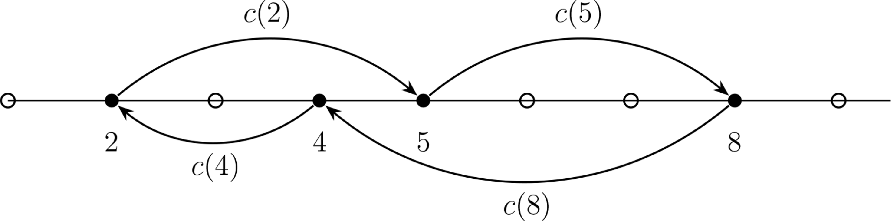
 A={2,4,5,8}
 σ(2)=5
 σ(4)=2
 σ(5)=8
 σ(8)=4

 g(k)=(k+1)α
 α=1,3
 N=104
 L=106
 X0≡100
 Z0≡100
 ρ
 ΛN
 16
 n=105
 fa,b(r)=1Γ(a)bara−1e−1br
 a=α+2
 b=100α+2

 g(k)=(k+1)α
 α=−1,−2
 fλ(r)=λe−λr
 λ=1100
 g(k)=(k+1)−2
 n=105
 n=106
 N=103
 n=106


