





1. Introduction
The geometry and analysis of triholomorphic maps and their moduli space is a challenging problem which has been attracting more and more attentions in both mathematics and physics. Triholomorphic maps appear naturally in high-dimensional gauge theory [Reference Chen6, Reference Donaldson and Thomas10, Reference Miguel Figueroa-O’Farrill, Köhl and Spence19]. They are closely related to the topological sigma models in 4 dimensions and hyperinstantons [Reference Anselmi and Fré1] and the classification of solutions to the 3 dimensional Beltrami equations for hydrodynamics [Reference Frè, Grassi and Sorin11]. They have been playing a very important role in understanding hyperKähler geometry [Reference Tian27]. To understand the sigma models and hyperintantons, it is natural to investigate boundary value problems for triholomorphic maps, see for instance, [Reference Frè, Grassi and Sorin11, Section 3, Section 6].
When the domain is a hyperKähler manifold, smooth triholomorphic maps are harmonic maps, e.g. Chen [Reference Chen6, Lemma 3.1] and weakly (respectively stationary) triholomorphic maps are weakly (respectively stationary) harmonic maps, e.g. Wang [Reference Wang28, Lemma 2.1]. The compactness problem and energy quantization for stationary triholomorphic maps from a closed domain was studied by Wang [Reference Wang28]. In the more general framework, when the domain manifold is merely almost hyper-Hermitian, the energy quantization for locally approximable triholomorphic maps from a closed domain was established by Bellettini-Tian [Reference Bellettini and Tian2].
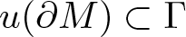
In this paper, we introduce a natural boundary value problem for triholomorphic maps from a compact almost hyper-Hermitian manifold with smooth boundary into a closed hyperKähler manifold, which maps the boundary to some geometrically natural closed supporting submanifold in the target space, called tri-isotropic submanifold. Then we establish partial regularity theory and energy quantization result in this boundary value setting of triholomorphic maps.
Let  $(M,g,i,j,k)$ be a compact and almost hyper-Hermitian manifold of dimension
 $4m$ with smooth non-empty boundary
 $\partial M$ and
 $(N,h,I,J,K)$ be a closed hyperKähler manifold of dimension
 $4n$. Here
 $i,j,k$ (respectively
 $I,J,K$) are three smooth almost complex structures compatible with the smooth Riemannian metric
 $g$ (respectively
 $h$) on
 $M$ (respectively
 $N$) and satisfy the quaternionic relation
 $ijk=-Id$ (respectively
 $IJK=-Id$). We denote by
 $\omega_i(\cdot,\cdot):=g(\cdot,i\cdot)$ the unique and non-degenerate 2-form associated with
 $g$ and
 $i$ on
 $M$. Similarly, we have the 2-forms
 $\omega_j,\omega_k$ on
 $M$ and the 2-forms
 $\Omega_I,\Omega_J,\Omega_K$ on
 $N$. Note that “hyperKähler” means that the 2-forms
 $\Omega_I,\Omega_J,\Omega_K$ are closed.
By Nash’s embedding theorem, we embed  $(N,h)$ isometrically into some Euclidean space
 $\mathbb{R}^{\mathcal{K}}$ for some
 $\mathcal{K}$. Consider the Sobolev space
 \begin{equation*}H^1\left(M,N\right):=\left\{v\in H^1(M,\mathbb{R}^\mathcal{K})\,:\, v(x)\in N \text{ for a.e. } x\in M\right\}.\end{equation*}
To proceed, we need some definitions.
Definition 1.1. A submanifold  $\Gamma$ of
 $(N,h,I,J,K)$ is called a tri-isotropic submanifold if
 $\Gamma$ is an isotropic submanifold of all three symplectic manifolds
 $(N,\Omega_I),(N,\Omega_J)$ and
 $(N,\Omega_K)$. In other words,
 $\Gamma$ is a submanifold vanishing all three Kähler forms on
 $N$.
Similarly to Lagrangian submanifolds of symplectic manifolds, a maximal tri-isotropic submanifold is called a tri-Lagrangian submanifold. The largest dimension of a tri-isotropic submanifold of  $N$ is
 $n$.
Now we give examples of tri-isotropic submanifolds and tri-Lagrangian submanifolds.
Example 1.2. Consider the following holomorphic symplectic form with respect to complex structure  $I$ on
 $N$
 \begin{equation*}
\Omega:=\Omega_J+\sqrt{-1}\cdot\Omega_K.
\end{equation*}
Suppose there exists a complex Lagrangian submanifold  $L$ of the symplectic manifold
 $(N,\Omega)$ with real dimension
 $2n$. It is elementary to verify
 \begin{equation*}\left(L,h':=h\llcorner L,I':=I\llcorner L,\Omega_I':=\Omega_I\llcorner L \right),\end{equation*}
is a Kähler manifold, where “ $\llcorner$” means restriction.
To begin with, we claim that  $I'$ is a smooth complex structure on
 $L$, i.e.,
 $I$ preserve the tangent bundle
 $TL$. For any
 $q\in L$ and
 $ X,Y\in T_qL\subset T_qN,$ the definition of Lagrangian submanifolds leads to
 \begin{equation*}
h(q)(X,J(Y))=\Omega_J(q)(X,Y)=0=\Omega_K(q)(X,Y)=h(q)(X,K(Y)),
\end{equation*}
which means  $J(T_qL)$ and
 $K(T_qL)$ is the subspace of the orthogonal complement of
 $T_qL$ with respect to the metric
 $h$, which is denoted by
 $T_q^ \perp L$. Notice that
 $J,K$ is linear isomorphism hence injective. Compare the dimensions between
 $T_qL$ and
 $T^\perp_qL$, we obtain
 \begin{equation*}J(T_qL)=T_q^ \perp L=K(T_qL).\end{equation*}
Then it is easy to see
 \begin{equation*}I'=(J\circ K)\llcorner L:TL\to TL,\end{equation*}
is a linear isomorphism.
Next, we show that  $(L,\Omega_I')$ is a symplectic manifold. It is sufficient to check that
 $\Omega_I'$ is closed and non-degenerate. Let
 $\mathfrak{I}:L\to N$ be the natural embedding map. Then
 \begin{equation*}d\Omega_I'=d(\mathfrak{I}^*\Omega_I)=\mathfrak{I}^*(d\Omega_I)=0,\end{equation*}
where  $\mathfrak{I}^*$ denotes the pull-back of
 $\mathfrak{I}$ and the closeness of
 $\Omega_I'$ is valid. Fix a point
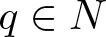 $q\in N$ and suppose
 $\Omega_I'(X,Y)=0$ holds for all
 $Y\in T_qL$, we assert that
 $X\in T_qL$ must be zero. By the definition of
 $\Omega_I'$,
 \begin{equation*}
\begin{aligned}
0=\Omega_I'(X,Y)&=\mathfrak{I}^*\Omega_I(X,Y)=\Omega_I(d\mathfrak{I}(X),d\mathfrak{I}(Y))=h(d\mathfrak{I}(X),I\circ d\mathfrak{I}(Y))\\
&=h(d\mathfrak{I}(X),d\mathfrak{I}\circ I(Y))=\mathfrak{I}^*h(X,I(Y))=h'(X,I(Y)).\\
\end{aligned}
\end{equation*}
Here,  $I\circ d\mathfrak{I}=d\mathfrak{I} \circ I$ is deduced from the fact that
 $I$ preserves
 $TL$ in local coordinates directly. Besides,
 $h'$ is the induced Riemannian metric hence non-degenerate. It is clear that
 $X=0$ from
 $I(T_qL)=T_qL$. As a corollary,
 $\Omega_I'(\cdot,\cdot)=h'(\cdot,I'\cdot)$.
Let  $\Gamma$ be a Lagrangian submanifold of
 $(L,\Omega_I')$. Then
 $\Gamma$ is a tri-isotropic submanifold of
 $N$ with dim
 $L=n$, which means that
 $\Gamma$ is actually a tri-Lagrangian submanifold of
 $N$.
Definition 1.3. Let  $(M,g,i,j,k)$ and
 $(N,h,I,J,K)$ be as above. Suppose that
 $\Gamma\subset N$ is a closed tri-isotropic submanifold with
 $1\le$ dim
 $\Gamma\le n$. A map
 $u\in H^1(M,N)$ is called a locally approximable triholomorphic map with respect to the tri-isotropic free boundary condition
 $u(\partial M)\subset \Gamma$ if
 $u$ satisfies the followings:
(i) Weakly triholomorphic maps equation:
 $du=I\circ du\circ i+J\circ du \circ j+K\circ du \circ k$.
(ii) Free boundary condition:
$du(x)(\nu(x))\perp T_{u(x)}\Gamma$ for a.e.
$x\in\partial M$, where
$\nu(x)$ is the outward unit normal vector at
$x\in\partial M$ and “
$\perp$” means orthogonal.(iii) Locally approximable condition:
$d(u^*\Omega)=0$ for every closed 2-form
$\Omega$ on
$N$.


Remark 1.4. For the locally approximable condition, we actually only need it for  $\Omega=\Omega_I,\Omega_J,\Omega_K$ in the present work.
Before proceeding, we explain that Definition 1.3 is a natural definition. To be more precise, we shall show that, when  $M$ is a hyperKähler manifold, a locally approximable triholomorphic map
 $u$ with respect to the tri-isotropic free boundary condition
 $u(\partial M)\subset \Gamma$ is a stationary harmonic map with respect to the free boundary condition
 $u(\partial M)\subset\Gamma$.
Let  $\phi\in C^\infty(M,\mathbb{R}^{\mathcal{K}})$ satisfy
 $\phi(x)\in T_{u(x)}N$ for a.e.
 $x\in M$ and
 $\phi(x)\in T_{u(x)}\Gamma$ for a.e.
 $x\in \partial M$. Such a vectorfield is called an admissible target variation vectorfield with respect to the free boundary condition
 $u(\partial M)\subset \Gamma$. Let
 $\Pi_N$ be the nearest point projection of some neighborhood of
 $N\subset\mathbb{R}^{\mathcal{K}}$. The variation of
 $u$ is defined as
 \begin{equation*}u_t:=\Pi_N(u+t\phi).\end{equation*}
According to the computations in [Reference Bellettini and Tian2] (see also [Reference Chen and Jia-Yu7, Proposition 2.2], [Reference Rivière and Tian23, Proposition II.1], [Reference Wang28, Lemma 2.1], [Reference Caniato and Rivière4, Lemma 3.2] for more details), we have for every admissible target variation vectorfield  $\phi$ with respect to the free boundary condition
 $u(\partial M)\subset \Gamma$
 \begin{align}
\frac{d}{dt}E\left(u_t\right)\Big|_{t=0}
&=\frac{1}{(2m-1)!}\left( -\int_{M}d\left(\omega_i^{2m-1}\wedge u^*(\iota_\phi\Pi_N^*\Omega_I)\right) \right.\cr
&\left.\quad +\int_{M}\left(d(\omega_i^{2m-1})\right)\wedge\left(u^*(\iota_\phi\Pi_N^*\Omega_I)\right)\right) \cr
&\quad +(\omega_j,J)-\text{term}+(\omega_k,K)-\text{term},
\end{align}
and
 \begin{equation*}
u^*(\iota_\phi\Pi_N^*\Omega_I)(X):=u^*\Pi_N^*\Omega_I(\phi,X)=u^*\Omega_I(\phi,X),
\end{equation*}
for all  $X\in C^\infty(M,TN)$ that are tangential along
 $u$ and fulfill the same boundary condition as
 $\phi$.
By the Stokes theorem and the definition of  $u$ and
 $\Gamma$ in Definition 1.3,
 \begin{equation*}
\int_{M}d\left(\omega_i^{2m-1}\wedge u^*(\iota_\phi\Omega_I)\right)=\int_{\partial M}\omega_i^{2m-1}\wedge u^*(\iota_\phi\Omega_I)=0.
\end{equation*}
The same result holds for  $(\omega_j,J)$-term and
 $(\omega_k,K)$-term. Moreover, by canonical calculations for the equations of weakly harmonic maps with respect to the free boundary conditions, l.h.s. of (1.1) is equal to
 \begin{equation*}
\int_{M}\left \lt \nabla u,\nabla\phi\right \gt \,\mathrm{d}Vol_g.
\end{equation*}
Consequently, we obtain (compare with [Reference Bellettini and Tian2, (32)])
 \begin{equation}
\begin{aligned}
&\int_{M}\left \lt \nabla u,\nabla\phi\right \gt \,\mathrm{d}Vol_g= \frac{1}{(2m-1)!}\int_{M}\left(d(\omega_i^{2m-1})\right)\wedge(u^*(\iota_\phi\Omega_I))\\
&\quad +\left(d(\omega_j^{2m-1})\right)\wedge(u^*(\iota_\phi\Omega_J))+\left(d(\omega_k^{2m-1})\right)\wedge(u^*(\iota_\phi\Omega_K)).
\end{aligned}
\end{equation}
As in [Reference Bellettini and Tian2, § 3.3], (1.2) yields a perturbation of the classical harmonic map equation with respect to the free boundary condition  $u(\partial M)\subset\Gamma$, namely
 \begin{equation}
\begin{cases}
\Delta_g u-A(u)(\nabla u,\nabla u)=f(x,u,\nabla u)\quad x\in M,\\
u(x)\in \Gamma,\ \dfrac{\partial u}{\partial \vec{n}}(x)\perp T_{u(x)}\Gamma\quad \text{for a.e.}\ x\in\partial M,
\end{cases}
\end{equation}
where  $A(\cdot,\cdot)$ is the second fundamental form of
 $N\hookrightarrow\mathbb{R}^\mathcal{K}$,
 $\Delta_g$ is the Laplace-Beltrami operator on
 $M$ which is defined by
 \begin{equation*}
\Delta_g:=-\frac{1}{\sqrt{|g|}}\frac{\partial {}}{\partial {x^l}}\left(\sqrt{|g|}g^{ls}\frac{\partial {}}{\partial {x^s}}\right),
\end{equation*}
 $f$ is smooth with respect to the three variables and
 $f$ has linear dependence on the first derivatives of
 $u$ and
 $\vec{n}(x)$ is the outward unit normal vector at
 $x\in\partial M$.
Provided that  $M$ is a hyperKähler manifold, in other words,
 $\omega_i,\omega_j,\omega_k$ are closed (see [Reference Nigel20, Lemma 6.8]), (1.2) reduces to
 \begin{equation}
\int_{M}\left \lt \nabla u,\nabla\phi\right \gt \,\mathrm{d}Vol_g=0.
\end{equation}
The integral identity (1.4) is exactly the one used for defining weakly harmonic maps with respect to the free boundary condition  $u(\partial M)\subset\Gamma$. Hence we extend [Reference Wang28, Lemma 2.1] to the case of free boundary conditions thanks to the natural definition given in Definition 1.3.
Notice that the above discussions do not rely on the locally approximable condition (iii) in Definition 1.3. It can be seen from [Reference Bellettini and Tian2] that the locally approximable condition plays a role like “stationarity”. In fact, from [Reference Rivière and Tian23, Proposition II.2], we know that the locally approximable condition implies that weakly triholomorphic maps are stationary harmonic maps under the hyperKähler assumption on  $M$. The same observation was made in [Reference Caniato and Rivière4, Lemma 3.3] for pseudoholomorphic maps on higher-dimensional domains. From this point of view, intuitively, we expect a map
 $u$ which is as in Definition 1.3 to be a stationary harmonic map with respect to free boundary condition
 $u(\partial M)\subset \Gamma$ when
 $M$ is a hyperKähler manifold.
Definition 1.5. ([Reference Scheven25, Definition 1.1])
A map  $u$
 $\in H^1\left(M,N\right)$ is called a stationary harmonic map with respect to the free boundary condition
 $u(\partial M)\subset \Gamma$ if it is a weakly harmonic map satisfying the free boundary condition
 $u(\partial M)\subset \Gamma$ and
 \begin{equation}
\frac{d}{dt}E(u\circ \Psi_t)\Big|_{t=0}=0,
\end{equation}
holds for all 1-parameter families of  $C^{\infty}$-diffeomorphisms
 $\Psi_t:M\to M$ satisfying
(i)  $\Psi_0=Id_M$, (ii)
 $\Psi_t(\partial M)\subset \partial M$.
The computation is similar to that of target variations (see also [Reference Bellettini and Tian2, Reference Rivière and Tian23]). Let  $X$ be a smooth vectorfield with compact support on
 $M$ and satisfy that
 $X\big|_{\partial M}$ is a vectorfield on
 $\partial M$, that is
 $X(p)\in T_p\partial M(\subset T_pM)$ for all
 $p\in\partial M$. Denote
 $\Psi_t:=Id_M+tX$ the corresponding 1-parameter families of domain variations. Then it is easy to see that
 $\Psi_t$ are admissible domain variations vectorfields in the sense of Definition 1.5, and without loss of generality, we can assume that the admissible diffeomorphisms are of this form. We have
 \begin{equation}
\begin{aligned}
&\frac{d}{dt}E\left(u\circ \Psi_t,M\right)\Big|_{t=0}=\frac{d}{dt}\int_{M}\left| \nabla(u\circ \Psi_t)\right|^2\,\mathrm{d}Vol_g\,\Big|_{t=0} \\
&=\frac{1}{(2m-1)!}\int_{M}\left(d(\omega_i^{2m-1})\right)\wedge(\iota_X (u^*\Omega_I))+(\omega_j,J)-\text{term}+(\omega_k,K)-\text{term},\\
&\le C(m,\omega_i,\omega_j,\omega_k)\int_M|X|\cdot|\nabla u|^2\,\mathrm{d}Vol_g,\\
&\le C(m,g,\omega_i,\omega_j,\omega_k)\left\Vert X\right\Vert_{L^\infty}\int_{\textrm{spt}(X)}|\nabla u|^2\,dx,
\end{aligned}
\end{equation}
which is deduced from the following two facts:
 \begin{equation}
\frac{d}{dt}(u\circ \Psi_t)^*\Omega_I\Big|_{t=0}=d\left(\iota_X (u^*\Omega_I)\right)+\iota_X\left(d(u^*\Omega_I)\right)=d\left(\iota_X (u^*\Omega_I)\right),
\end{equation}
and
 \begin{equation}
\int_{M}d\left((\omega_i^{2m-1})\wedge(\iota_X (u^*\Omega_I))\right)=\int_{\partial M}(\omega_i^{2m-1})\wedge\left(\iota_X (u^*\Omega_I)\right)=0.
\end{equation}
If  $\omega_i,\omega_j,\omega_k$ are closed 2-forms, we immediately obtain that
 $u$ is a stationary harmonic map with respect to the free boundary condition
 $u(\partial M)\subset \Gamma$ as what we have anticipated.
Our main result is as follows:
Theorem 1.6 Let
 \begin{equation*}
u_l:(M,g,i,j,k)\to\left(N\hookrightarrow \mathbb{R}^\mathcal{K},h,I,J,K\right)\ \text{for }\ l=1,2,\cdots
\end{equation*}
be a sequence of locally approximable triholomorphic maps with respect to the tri-isotropic free boundary condition  $u_l\left(\partial M\right)\subset \Gamma$, and with a uniformly bounded
 $W^{2,1}$ norm, that is:
 \begin{equation*}
\left\Vert u_l\right\Vert_{W^{2,1}(M)}\le \Upsilon
\end{equation*}
for some universal constant  $\Upsilon \gt 0$. If
 $u_l\rightharpoonup u$ weakly in
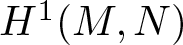 $H^1(M,N)$ with a uniform energy bound
 $\Lambda \gt 0$, then
 \begin{equation*}
|\nabla u_l|^2\,\mathrm{d}Vol_g\rightharpoonup|\nabla u|^2\,\mathrm{d}Vol_g+\nu \quad \text{as Radon measures on } M,
\end{equation*}
where  $u$ is a weakly triholomorphic map with respect to the tri-isotropic free boundary condition
 $u(\partial M)\subset \Gamma$ and is smooth away from a closed,
 $\left(4m-2\right)$-rectifiable set
 $\Sigma$ with
 $\mathscr{H}^{4m-2}\left(\Sigma\right) \lt \infty.$
Moreover,  $\nu$ is a non-negative Radon measure on
 $M$ of the form
 \begin{equation}
\nu=\Theta(x)\mathscr{H}^{4m-2}\llcorner\Sigma.
\end{equation}
Lastly, for  $\mathscr{H}^{4m-2}$-a.e.
 $x\in \Sigma\cap \partial M$, we have the following energy identity:
 \begin{equation*}
\Theta(x)=\sum\limits_{s=1}^{L_{x}}E(\phi_s)+\sum\limits_{p=1}^{L_{x}'}E(\varphi_p),
\end{equation*}
where  $\phi_s:S^2\to N$ is a smooth, non-constant harmonic 2-sphere for
 $s=1,\cdots,L_{x}$ and
 $\varphi_p:B^2\to N$ is a smooth, non-constant harmonic 2-disc with respect to the free boundary condition
 $\varphi_p(\partial B^2)\subset \Gamma$ for
 $p=1,\cdots,L_{x}'$.
The paper is organized as follows. In Section 2, we derive an almost-monotonicity formula in the boundary setting. In Section 3, we establish partial regularity theory in the boundary setting, including the  $\varepsilon$-regularity (see Theorem 3.6) and a gradient estimate (see Proposition 3.8). In Section 4, we complete the proof of Theorem 1.6.
2. Almost-monotonicity formula
In this section, we will derive an almost-monotonicity formula in the boundary setting. In the spirit of the interior case [Reference Bellettini and Tian2, Proposition 1], we arrive at an almost-monotonicity formula for locally approximable triholomorphic maps  $u$ with tri-isotropic free boundary condition. Set
 \begin{align*}
B_{R}(x_0)&=\left\{x\in\mathbb{R}^{4m}:|x-x_0| \lt R\right\};\\
B^+_{R}(x_0)&=\{x\in\mathbb{R}^{4m}:|x-x_0| \lt R,x^{(4m)}\ge0\};\\
\partial^0B^+_{R}(x_0)&=B_{R}^+(x_0)\cap \{x\in\mathbb{R}^{4m}:x^{(4m)}=0\};
\end{align*}
where  $x^{(4m)}$ denotes the
 $(4m)$th coordinate of
 $x$. When
 $x_0=0,$ we use
 $B_R,B_R^+$ and
 $\partial^0B^+_{R}$ for simplicity. Firstly, we have
Proposition 2.1. There exists  $r_0 \gt 0$ such that for any
 $x\in \partial M$ and
 $0 \lt r \lt r_0$ the following quantity is monotonically decreasing in weak sense as
 $r\downarrow 0:$
 \begin{equation}
\frac{(1+(4m-2)r)}{r^{4m-2}}\left[\int_{B_r^+(x)}(\alpha_1^{2m-1})\wedge u^*\Omega_I+(\alpha_2^{2m-1})\wedge u^*\Omega_J+(\alpha_3^{2m-1})\wedge u^*\Omega_K\right],
\end{equation}
where  $\alpha_1,\alpha_2,\alpha_3$ stand for the standard Kähler forms on the
 $m$-dimensional quaternionic vector space
 $\mathbb{H}^m$. This immediately yields the following almost-monotonicity formula for the energy ratio
 $:$
 \begin{equation*}
\frac{1}{r^{4m-2}}\int_{B_r^+(x)}|\nabla u|^2\,\mathrm{d}Vol_g=f(r)+O(rf(r)) \quad \text{with } f \text{a non-decreasing function of r}.
\end{equation*}
Proof. The proof is quite similar to that of [Reference Bellettini and Tian2, Proposition 1] except from applying some minor modifications. Note that for any  $(4m-3)$-form
 $\eta$ on
 $\partial M$, we have
 \begin{equation}
\int_{\partial M}\eta\wedge u^*\Omega_I=\int_{\partial M}\eta\wedge u^*\Omega_J=\int_{\partial M}\eta\wedge u^*\Omega_K=0.
\end{equation}
To see (2.2), as  $u$ satisfies the free boundary condition
 $u(\partial M)\subset \Gamma$ and
 $\Gamma$ is tri-isotropic, we have
 \begin{equation}
\iota^*_{\partial M}(u^*\Omega_I)=\iota^*_{\partial M}(u^*\Omega_J)=\iota^*_{\partial M}(u^*\Omega_K)=0 \quad \text{on } \partial M.
\end{equation}
For every subset  $A$ of
 $M$, we denote
 $\partial^0A:=\partial A\cap \partial M$ and
 $\partial^+A:=\partial A \backslash \partial^0A$. For each case in the proof of [Reference Bellettini and Tian2, Proposition 1], the calculation needs to be modified by (2.2) in only one place.
For Case 1 in the proof of [Reference Bellettini and Tian2, Proposition 1],
 \begin{equation*}
\begin{aligned}
&\frac{1}{R^{4m-2}}\int_{B_R^+}(\alpha_1^{2m-1})\wedge u^*\Omega_I-\frac{1}{s^{4m-2}}\int_{B_s^+}(\alpha_1^{2m-1})\wedge u^*\Omega_I\\
&=\int_{\partial B_R^+}\frac{\iota_{x\partial_x}(\alpha_1^{2m-1})}{(4m-2)R^{4m-2}}\wedge u^*\Omega_I-\int_{\partial B_s^+}\frac{\iota_{x\partial_x}(\alpha_1^{2m-1})}{(4m-2)s^{4m-2}}\wedge u^*\Omega_I
\end{aligned}
\end{equation*}
 \begin{equation*}
\begin{aligned}
&=\int_{\partial^+ B_R^+}\frac{\iota_{x\partial_x}(\alpha_1^{2m-1})}{(4m-2)|x|^{4m-2}}\wedge u^*\Omega_I-\int_{\partial^+ B_s^+}\frac{\iota_{x\partial_x}(\alpha_1^{2m-1})}{(4m-2)|x|^{4m-2}}\wedge u^*\Omega_I\\
&+\int_{\partial^0 B_R^+}\frac{\iota_{x\partial_x}(\alpha_1^{2m-1})}{(4m-2)R^{4m-2}}\wedge u^*\Omega_I-\int_{\partial^0 B_s^+}\frac{\iota_{x\partial_x}(\alpha_1^{2m-1})}{(4m-2)s^{4m-2}}\wedge u^*\Omega_I\\
\end{aligned}
\end{equation*}
 \begin{equation*}
\begin{aligned}
&\stackrel{(2.2)}{=\!=\!=}\int_{\partial^+ B_R^+}\frac{\iota_{x\partial_x}(\alpha_1^{2m-1})}{(4m-2)|x|^{4m-2}}\wedge u^*\Omega_I-\int_{\partial^+ B_s^+}\frac{\iota_{x\partial_x}(\alpha_1^{2m-1})}{(4m-2)|x|^{4m-2}}\wedge u^*\Omega_I\\
&+\int_{\partial^0 B_R^+}\frac{\iota_{x\partial_x}(\alpha_1^{2m-1})}{(4m-2)|x|^{4m-2}}\wedge u^*\Omega_I-\int_{\partial^0 B_s^+}\frac{\iota_{x\partial_x}(\alpha_1^{2m-1})}{(4m-2)|x|^{4m-2}}\wedge u^*\Omega_I\\
&=\int_{\partial(B_R^+\backslash B_s^+)}\frac{\iota_{x\partial_x}(\alpha_1^{2m-1})}{(4m-2)|x|^{4m-2}}\wedge u^*\Omega_I\\
&=\int_{B_R^+\backslash B_s^+}d\left(\frac{\iota_{x\partial_x}(\alpha_1^{2m-1})}{(4m-2)|x|^{4m-2}}\right)\wedge u^*\Omega_I=\int_{B_R^+\backslash B_s^+}\frac{(\alpha_1^{2m-1})_{\textrm{tan}}}{|x|^{4m-2}}\wedge u^*\Omega_I.
\end{aligned}
\end{equation*}
For Case 2 in the proof of [Reference Bellettini and Tian2, Proposition 1],
 \begin{equation*}
\begin{aligned}
0&\le\int_{B_R^+\backslash B_s^+}d\left( \frac{\iota_{x\partial_x}(\alpha_1^{2m-1})}{(4m-2)|x|^{4m-2}}+\frac{\iota_{x\partial_x}(\alpha_1^{2m-1})}{|x|^{4m-3}}\right)\wedge u^*\Omega_I\\
&=\int_{\partial (B_R^+\backslash B_s^+)}\left( \frac{\iota_{x\partial_x}(\alpha_1^{2m-1})}{(4m-2)|x|^{4m-2}}+\frac{\iota_{x\partial_x}(\alpha_1^{2m-1})}{|x|^{4m-3}}\right)\wedge u^*\Omega_I\\
&\stackrel{(2.2)}{=\!=\!=}\int_{\partial B_R^+}\left( \frac{\iota_{x\partial_x}(\alpha_1^{2m-1})}{(4m-2)R^{4m-2}}+\frac{\iota_{x\partial_x}(\alpha_1^{2m-1})}{R^{4m-3}}\right)\wedge u^*\Omega_I\\
\end{aligned}
\end{equation*}
 \begin{equation*}
\begin{aligned}
&-\int_{\partial B_s^+}\left( \frac{\iota_{x\partial_x}(\alpha_1^{2m-1})}{(4m-2)s^{4m-2}}+\frac{\iota_{x\partial_x}(\alpha_1^{2m-1})}{s^{4m-3}}\right)\wedge u^*\Omega_I\\
&=\frac{(1+(4m-2)R)}{(4m-2)R^{4m-2}}\int_{\partial B_R^+}\iota_{x\partial_x}(\alpha_1^{2m-1})\wedge u^*\Omega_I\\
& -\frac{(1+(4m-2)s)}{(4m-2)s^{4m-2}}\int_{\partial B_s^+}\iota_{x\partial_x}(\alpha_1^{2m-1})\wedge u^*\Omega_I\\
&=\frac{(1+(4m-2)R)}{R^{4m-2}}\int_{B_R^+}(\alpha_1^{2m-1})\wedge u^*\Omega_I-\frac{(1+(4m-2)s)}{s^{4m-2}}\int_{B_s^+}(\alpha_1^{2m-1})\wedge u^*\Omega_I.
\end{aligned}
\end{equation*}
The remaining proof follows from applying similar arguments as in the proof [Reference Bellettini and Tian2, Proposition 1], so we omit it.
Moreover, it is straightforward to verify the following immediate consequences of almost monotonicity.
(i) For every
$x\in\partial M,$ the density of
$u$ at
$x$ defined by
\begin{equation*}
\Theta(u,x):=\lim\limits_{r\to 0^+}\frac{1}{r^{4m-2}}\int_{B^+_r(x)}|\nabla u|^2\,\mathrm{d}Vol_g,
\end{equation*}exists.
(ii)
$\Theta(u,x)$ is an upper semi-continuous function of
$x$.(iii) There exist
$r_0 \gt 0$ and
$C \gt 0$, depending only on the geometric data, so that whenever
$x\in \partial M$ and
$0 \lt r \lt r_0$, we have
\begin{equation*}
\frac{1}{r^{4m-2}}\int_{B_r^+(x)}|\nabla u|^2\,\mathrm{d}Vol_g\ge \Theta(u,x)-Cr.
\end{equation*}(iv) By the compactness of
$\partial M$, there exist
$R_0 \gt 0$ and
$C \gt 0$, depending only on the geometric data, so that whenever
$x\in \partial M$ and
$0 \lt r_1 \lt r_2 \lt R_0$, we have
\begin{equation*}
\frac{1}{r_1^{4m-2}}\int_{B_{r_1}^+(x)}|\nabla u|^2\,\mathrm{d}Vol_g\le \frac{1+Cr_2}{r_2^{4m-2}}\int_{B_{r_2}^+(x)}|\nabla u|^2\, \mathrm{d}Vol_g.
\end{equation*}The same holds for
$y\in B_{R_0}^+(x)\backslash \partial^0 B_{R_0}^+(x)$ as long as
$B_{r_2}^+(y)=B_{r_2}(y)\subset B_{R_0}^+(x)$.


3. Partial regularity
In this section, we will establish partial regularity theory of  $u$ in the boundary setting, inspired by Scheven’s work [Reference Scheven24, Reference Scheven25]. Without loss of generality (up to a dilation), we set
 $R_0=1$ in (iv) of Corollary 2.2.
Lemma 3.1. (cf. [Reference Scheven24, Korollar 1.13], [Reference Scheven25, Corollary 1.3])
There exists a constant  $C \gt 0$, depending only on the geometric data, such that for all locally approximable triholomorphic maps
 $u$ with respect to the tri-isotropic free boundary condition
 $u(\partial M)\subset \Gamma$, it holds that
 \begin{equation*}
\sup\limits_{x\in B^+_{1/2}\atop 0 \lt r \lt 1-|x|}\frac{1}{r^{4m-2}}\int_{B^+_r(x)}|\nabla u|^2\,\mathrm{d}Vol_g\le C \int_{B^+_{1}}|\nabla u|^2\,\mathrm{d}Vol_g.
\end{equation*}
Proof. Consider  $x\in \partial^0 B_{1/2}^+$ first. If
 $0 \lt r \lt 1/2,$ it holds from (iv) of Corollary 2.2
 \begin{equation*}
\begin{aligned}
\frac{1}{r^{4m-2}}\int_{B^+_r(x)}|\nabla u|^2\,\mathrm{d}Vol_g&\le (1+C/2)2^{4m-2}\int_{B^+_{1/2}(x)}|\nabla u|^2\,\mathrm{d}Vol_g\\ &\le (1+C/2)2^{4m-2}\int_{B^+_{1}}|\nabla u|^2\,\mathrm{d}Vol_g.
\end{aligned}
\end{equation*}
If  $1/2\le r \lt 1-|x|$, then
 \begin{equation*}
\frac{1}{r^{4m-2}}\int_{B^+_r(x)}|\nabla u|^2\,\mathrm{d}Vol_g\le 2^{4m-2}\int_{B^+_{1}}|\nabla u|^2\,\mathrm{d}Vol_g.
\end{equation*}
Next, we assume  $x=\left(x',x^{(4m)}\right)$ with
 $d:=x^{(4m)} \gt 0$. If
 $d\le r \lt 1/4$, we have
 \begin{equation*}
\begin{aligned}
\frac{1}{r^{4m-2}}\int_{B^+_r(x)}|\nabla u|^2\,\mathrm{d}Vol_g&\le \frac{1}{r^{4m-2}}\int_{B^+_{r+d}\left((x',0)\right)}|\nabla u|^2\,\mathrm{d}Vol_g, \\
\end{aligned}
\end{equation*}
 \begin{equation*}
\begin{aligned}
&\le \frac{2^{4m-2}}{(2r)^{4m-2}}\int_{B^+_{2r}\left((x',0)\right)}|\nabla u|^2\,\mathrm{d}Vol_g\\
&\le 2^{4m-2}(1+C)\left(1-|(x',0)|\right)^{2-4m}\int_{B^+_{\left(1-|(x',0)|\right)}\left((x',0)\right)}|\nabla u|^2\,\mathrm{d}Vol_g\\
&\le 4^{4m-2}(1+C)\int_{B^+_{1}}|\nabla u|^2\,\mathrm{d}Vol_g.
\end{aligned}
\end{equation*}
If  $1/4\le r \lt 1-|x|$, we arrive at
 \begin{equation*}
\frac{1}{r^{4m-2}}\int_{B^+_r(x)}|\nabla u|^2\,\mathrm{d}Vol_g\le 4^{4m-2}\int_{B^+_{1}}|\nabla u|^2\,\mathrm{d}Vol_g.
\end{equation*}
If  $r \lt d$, we obtain
 \begin{align*}
&\frac{1}{r^{4m-2}}\int_{B^+_r(x)}|\nabla u|^2\,\mathrm{d}Vol_g\\
&=\frac{1}{r^{4m-2}}\int_{B_r(x)}|\nabla u|^2\,\mathrm{d}Vol_g
\le \frac{1+Cd}{d^{4m-2}}\int_{B_d(x)}|\nabla u|^2\,\mathrm{d}Vol_g.
\end{align*}
If  $1/4\le d \lt 1/2$,
 \begin{equation*}
\frac{1+Cd}{d^{4m-2}}\int_{B_d(x)}|\nabla u|^2\,\mathrm{d}Vol_g\le (1+C/2)4^{4m-2}\int_{B^+_{1}}|\nabla u|^2\,\mathrm{d}Vol_g.
\end{equation*}
If  $0 \lt d \lt 1/4$,
 \begin{equation*}
\begin{aligned}
\frac{1+Cd}{d^{4m-2}}\int_{B_d(x)}|\nabla u|^2\,\mathrm{d}Vol_g&\le \frac{1+C/4}{d^{4m-2}}\int_{B^+_{2d}\left((x',0)\right)}|\nabla u|^2\,\mathrm{d}Vol_g\\
&\le(1+C/4)2^{4m-2}(1+C)\left(1-|(x',0)|\right)^{2-4m}\\
&\quad \times \int_{B^+_{\left(1-|(x',0)|\right)}\left((x',0)\right)}|\nabla u|^2\,\mathrm{d}Vol_g\\
&\le (1+C/4)(1+C)4^{4m-2}\int_{B^+_{1}}|\nabla u|^2\,\mathrm{d}Vol_g.
\end{aligned}
\end{equation*}
Lemma 3.2. (cf. [Reference Scheven24, Satz 2.1], [Reference Scheven25, Lemma 3.1])
There exists a constant  $\varepsilon_0 \gt 0$, depending only on the geometric data, such that for all locally approximable triholomorphic maps
 $u$ with respect to the tri-isotropic free boundary condition
 $u(\partial M)\subset \Gamma$ and
 \begin{equation}
\sup\limits_{x\in B^+_{1/2}\atop 0 \lt r \lt 1/2-|x|}\frac{1}{r^{4m-2}}\int_{B^+_r(x)}|\nabla u|^2\,\mathrm{d}Vol_g\le \varepsilon_0,
\end{equation}
it holds  $\textrm{dist}^N(u(x),\Gamma)\le C\varepsilon_0^{1/2}$ for all
 $x\in B_{1/4}^+$ with a constant
 $C \gt 0$, depending only on the geometric data.
Proof. From the interior regularity for locally approximable triholomorphic maps [Reference Bellettini and Tian2, § 3.3], we know that  $u$ is smooth in the interior of
 $B^{+}_{1/2}$ and the following interior gradient estimate holds (see [Reference Bellettini and Tian2, (33)]):
 \begin{equation*}
\left|\nabla u\right|\le\frac{C\sqrt{\varepsilon_0}}{\textrm{dist}\left(x,\partial^0 B^+_{1/2}\right)}.
\end{equation*}
Then the proof is almost identical to that of [Reference Scheven25, Lemma 3.1].
On account of Lemma 3.2, we may choose  $\delta \gt 0$ sufficiently small such that
(i) The geodesic reflection
$\sigma$ across
$\Gamma$ defined on the
$\delta$-neighborhood of
$\Gamma\subset N$
\begin{equation*}U_\delta:=\left\{x\in N:\textrm{dist}^N(x,\Gamma) \lt \delta\right\}\end{equation*}is a diffeomorphism.
(ii) If the scaled energies of
$u$ are sufficiently small, that is (3.1) holds, then
$u(B^+_{1/4})\subset U_\delta$.


The geodesic reflection  $\sigma$ across
 $\Gamma$ is defined as follows: for
 $y\in U_\delta$, the nearest point
 $\pi(y)\in\Gamma$ is uniquely defined and connected to
 $y$ by a unique shortest geodesic. Hence
 \begin{equation*}
\sigma:U_\delta\to U_\delta,\ y=\exp_{\pi(y)}(v)\longmapsto\exp_{\pi(y)}(-v),
\end{equation*}
where  $v\in T_{\pi(y)}N$ is uniquely determined by the constraint condition
 $|v|=\textrm{dist}^N(y,\Gamma)$. Hence we can extend
 $u$ onto
 $B_{1/4}$ by
 $\sigma$ as follows:
 \begin{equation*}
\bar{u}(x):=\begin{cases}
u(x)&,x\in B_{1/4}^+,\\
\sigma(u(\rho(x)))&,x\in B_{1/4}^-,
\end{cases}
\end{equation*}
where  $\rho(x)$ is the reflection
 \begin{equation*}
\rho\left(x=\left(x^1,\cdots,x^{4m-1},x^{4m}\right)\right):=\left(x^1,\cdots,x^{4m-1},-x^{4m}\right), \,x\in B_{1/4}.
\end{equation*}
Then we extend the Riemannian metric  $g$ onto
 $B_{1/4}$ by
 $\rho$ as follows:
 \begin{equation*}
\bar{g}(x)(X,Y):=\begin{cases}
g(x)(X,Y)&,x\in B_{1/4}^+,\\
\rho^*g(x)(X,Y)\\
\quad =g(\rho(x))(d\rho(x)(X),d\rho(x)(Y))&,x\in B_{1/4}^-,
\end{cases}
\text{for }\forall\,X,Y\in T_xB_{1/4}.
\end{equation*}
Such extension of the Riemannian metric is also used to prove the partial regularity for stationary harmonic maps with free boundary, see [Reference Scheven24, (2.4)].
In the local coordinates  $\bar{g}=(\bar{g}_{ls})$, for
 $x\in B^-_{1/4}$,
 \begin{equation}
\bar{g}_{ls}(x)=(-1)^{\delta_{l m'}+\delta_{s m'}}g_{ls}(\rho(x)),
\end{equation}
where  $m':=4m$ for simplicity and
 \begin{equation*}
\delta_{ls}=\begin{cases}
1&, \text{if } l=s,\\
0&, \text{if } l\not=s,
\end{cases}
\end{equation*}
denotes the Kronecker symbol. By the nature of the coordinates system at the boundary,  $g_{m'm'}=1$ in the neighborhood of
 $\partial M$ which yields
 $\bar{g}_{m'm'}$ is smooth. By definition, for every
 $x\in\partial M$ the normal vector
 $\nu(x)$ is orthogonal to
 $T_x(\partial M)$. Therefore, we have
 $g_{l m'}=g_{m'l}=0$ for
 $l=1,\cdots,m'-1$ and
 \begin{equation*}
\frac{\partial g_{l m'}}{\partial x_{m'}}=\frac{\partial}{\partial x_{m'}}\left \lt \partial_l,\partial_{m'}\right \gt =\left \lt \nabla_{\partial_{m'}}\partial_l,\partial_{m'}\right \gt +\left \lt \partial_l,\nabla_{\partial_{m'}}\partial_{m'}\right \gt ,
\end{equation*}
where  $\nabla$ is the Levi-Civita connection on
 $(M,g)$. By the geodesic construction of the neighborhood,
 $\nabla_{\partial_{m'}}\partial_{m'}=0$ and we obtain
 \begin{equation*}
\frac{\partial g_{l m'}}{\partial x_{m'}}=\left \lt \nabla_{\partial_{m'}}\partial_l,\partial_{m'}\right \gt .
\end{equation*}
From the properties of the Levi-Civita connection, we know for any three smooth vectorfields  $X,Y,Z$ defined on
 $M$
 \begin{align*}
\left \lt Z,\nabla_YX\right \gt &=\frac{1}{2}\left(X\left \lt Y,Z\right \gt +Y\left \lt Z,X\right \gt -Z\left \lt X,Y\right \gt -\left \lt [X,Z],Y\right \gt \right.\\
&\left.\quad -\left \lt [Y,Z],X\right \gt -\left \lt [X,Y],Z\right \gt \right).
\end{align*}
Hence,
 \begin{equation*}
\left \lt \nabla_{\partial_{m'}}\partial_l,\partial_{m'}\right \gt =\frac{1}{2}\frac{\partial g_{m'm'}}{\partial x_{l}}=0,
\end{equation*}
which means that  $g_{l m'}=g_{m'l}=0$ near the boundary such that
 $\bar{g}_{l m'}$ and
 $\bar{g}_{m' l}$ are smooth for
 $l=1,\cdots,m'-1$. Moreover,
 $\bar{g}$ is continuous and the extension is actually the even extension.
Owing to isometrically embedding  $N\hookrightarrow\mathbb{R}^{\mathcal{K}}$, we still use
 $h$ to denote the metric on
 $TN$ which is induced by the Euclidean metric on
 $\mathbb{R}^\mathcal{K}$. Then we define
 \begin{equation*}
\bar{h}(x):=\begin{cases}
h(\bar{u}(x))&,x\in B_{1/4}^+,\\
\sigma^*h(\bar{u}(x))&,x\in B_{1/4}^-,
\end{cases}
\end{equation*}
and
 \begin{equation*}
\Sigma(x):=\nabla\sigma\left(\bar{u}(x)\right).
\end{equation*}
According to the arguments in [Reference Scheven25, § 3], we know 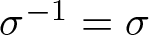 $\sigma^{-1}=\sigma$,
 $\Sigma^{-1}(x)=\Sigma(\rho(x))$ and for
 $x_0\in\partial^0B^+_{1/4}$, we have
 \begin{equation*}
\Sigma(x_0)=\Pi_\Gamma(u(x_0))-\Pi^\perp_\Gamma(u(x_0)),
\end{equation*}
where  $\Pi_\Gamma(y)$ and
 $\Pi^\perp_\Gamma(y)$ for
 $y\in \Gamma$ are the orthogonal projections from
 $T_yN$ on
 $T_y\Gamma$ and
 $T_y^\perp \Gamma$, respectively.
The covariant derivative of an  $H^1$-vectorfield
 $V$ tangential to
 $N$ along
 $\bar{u}$ is defined by
 \begin{equation*}
\nabla^{\bar{h}}V(x):=\begin{cases}
\nabla^NV(x)&,x\in B_{1/4}^+,\\
\Sigma(\rho(x))\nabla^N(\Sigma(x)V(x))&,x\in B_{1/4}^-,
\end{cases}
\end{equation*}
with the Levi-Civita connection  $\nabla^N$ on
 $(N,h)$.
Then we obtain the following equation for the extended map  $\bar{u}$.
Lemma 3.3. (cf. [Reference Scheven24, Lemma 2.4], [Reference Scheven25, Lemma 3.2])
Let  $V\in H^1\cap L^\infty(B_{1/4},TN)$ be a vectorfield tangential to
 $N$ along
 $\bar{u}$ with compact support in
 $B_{1/4}$ and
 $V(x)\in T_{\bar{u}(x)}N$ for a.e.
 $x\in B_{1/4}$. Then it holds
 \begin{equation}
\int_{B_{1/4}}\nabla \bar{u}\cdot_{\bar{h}}^{\bar{g}}\nabla^{\bar{h}}V\,\mathrm{d}Vol_{\bar{g}}=\int_{B_{1/4}}\bar{f}(x,\bar{u},\nabla \bar{u})\cdot_{\bar{h}}V\,\mathrm{d}Vol_{\bar{g}},
\end{equation}
where ‘ $\cdot_{\bar{h}}^{\bar{g}}$’ stands for the Hilbert-Schmidt scalar product with respect to the metric
 $\bar{h}$ on
 $TN$ and
 \begin{equation*}
\bar{f}(x,y,\xi):=\begin{cases}
f(x,y,\xi)&,x\in B^+_{1/4},\\
\Sigma(\rho(x))\cdot f\left(\rho(x),\sigma(y),\Sigma(x)\xi(x)\nabla \rho(\rho(x))\right)&,x\in B^-_{1/4}.
\end{cases}
\end{equation*}
Here,  $f$ is the function in (1.3).
Proof. As in the proof of [Reference Scheven25, Lemma 3.2]. We decompose the vectorfield  $V$ into two parts
 $V=V_e+V_a$ for
 $x\in B_{1/4}$
 \begin{equation*}
\begin{aligned}
V_e(x)&:=\frac{1}{2}\left[V(x)+\Sigma(\rho(x))V(\rho(x))\right]\\
V_a(x)&:=\frac{1}{2}\left[V(x)-\Sigma(\rho(x))V(\rho(x))\right]
\end{aligned}
\end{equation*}
Then it holds
 \begin{equation*}
V_e(\rho(x))=\Sigma(x)V_e(x)\ \text{and }\ V_a(\rho(x))=-\Sigma(x)V_a(x).
\end{equation*}
It is clear that for  $x_0\in\partial^0B^+_{1/4}$,
 $V_e(x_0)\in T_{u(x_0)}\Gamma$ and
 $V_e|_{B^+_{1/4}}$ is an admissible target variation vectorfield for
 $\bar{u}|_{B^+_{1/4}}$ with respect to the free boundary condition
 $\bar{u}(\partial^0B^+_{1/4})\subset \Gamma$. Hence from (1.2) and (1.3) we have
 \begin{equation*}
\int_{B^+_{1/4}}\nabla \bar{u}\cdot_{\bar{h}}^{\bar{g}}\nabla^{\bar{h}}V_e\,\mathrm{d}Vol_{\bar{g}}=\int_{B^+_{1/4}}\nabla u\cdot^{g}\nabla^{N}V_e\,\mathrm{d}Vol_g=\int_{B^+_{1/4}}f(x,u,\nabla u)\cdot_h V_e\mathrm{d}Vol_g.
\end{equation*}
By the definition of  $\bar{h}$ and
 $\nabla^{\bar{h}}$, we have
 \begin{equation*}
\begin{aligned}
\int_{B^-_{1/4}}\nabla \bar{u}\cdot_{\bar{h}}^{\bar{g}}\nabla^{\bar{h}}V_e\,\mathrm{d}Vol_{\bar{g}}&=\int_{B^-_{1/4}}\Sigma(x)\nabla \bar{u}(x)\cdot^{\bar{g}(x)}\nabla^{N}(\Sigma(x)V_e(x))\,\mathrm{d}Vol_{\bar{g}}\\
&=\int_{B^-_{1/4}}\nabla [u(\rho(x))]\cdot^{\bar{g}(x)}\nabla^{N}[V_e(\rho(x))]\,\mathrm{d}Vol_{\bar{g}}\\
&\stackrel{(3.2)}{=\!=\!=}\int_{B^-_{1/4}}\nabla u(\rho(x))\cdot^{g(\rho(x))}\nabla^NV_e(\rho(x))\,\mathrm{d}Vol_g\\
&=\int_{B^+_{1/4}}\nabla u\cdot^g\nabla^NV_e\,\mathrm{d}Vol_g.
\end{aligned}
\end{equation*}
Analogously, one can easily show that
 \begin{equation*}
\int_{B^-_{1/4}}\nabla \bar{u}\cdot_{\bar{h}}^{\bar{g}}\nabla^{\bar{h}}V_a\,\mathrm{d}Vol_{\bar{g}}=-\int_{B^+_{1/4}}\nabla \bar{u}\cdot_{\bar{h}}^{\bar{g}}\nabla^{\bar{h}}V_a\,\mathrm{d}Vol_{\bar{g}}.
\end{equation*}
Next, we may check
 \begin{align*}
\int_{B^-_{1/4}}\bar{f}(x,\bar{u},\nabla \bar{u})\cdot_{\bar{h}}V_e\,\mathrm{d}Vol_{\bar{g}}&=\int_{B^+_{1/4}}\bar{f}(x,\bar{u},\nabla \bar{u})\cdot_{\bar{h}}V_e\,\mathrm{d}Vol_{\bar{g}}\\
&=\int_{B^+_{1/4}}f(x,u,\nabla u)\cdot_h V_e\mathrm{d}Vol_g.
\end{align*}
Because of the definition of  $\bar{f}$,
 \begin{equation*}
\begin{aligned}
\int_{B^-_{1/4}}\bar{f}(x,\bar{u},\nabla \bar{u})\cdot_{\bar{h}}V_e\,\mathrm{d}Vol_{\bar{g}}&=\int_{B^-_{1/4}}\Sigma(x)\bar{f}(x,\bar{u},\nabla \bar{u})\cdot \Sigma(x)V_e(x)\,\mathrm{d}Vol_{\bar{g}}\\
&=\int_{B^-_{1/4}}f\left(\rho(x),u(\rho(x)),\nabla u(\rho(x))\right)\cdot V_e(\rho(x))\,\mathrm{d}Vol_{\bar{g}}\\
&=\int_{B^+_{1/4}}f(x,u,\nabla u)\cdot_h V_e\,\mathrm{d}Vol_g.
\end{aligned}
\end{equation*}
Similarly, we can acquire
 \begin{equation*}
\int_{B^-_{1/4}}\bar{f}(x,\bar{u},\nabla \bar{u})\cdot_{\bar{h}}V_a\,\mathrm{d}Vol_{\bar{g}}=-\int_{B^+_{1/4}}f(x,u,\nabla u)\cdot_h V_a\,\mathrm{d}Vol_g.
\end{equation*}
Now, the statement follows by a direct check.
Remark 3.4. It is obvious that 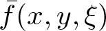 $\bar{f}(x,y,\xi)$ still depends linearly on
 $\xi$ and
 \begin{equation*}
|\bar{f}(x,y,\xi)|\le C(1+|\xi|)\ \text{for all }\ x\in B_{1/4}, y\in N, \xi \in \mathbb{R}^{m'*}\otimes TN,
\end{equation*}
with a constant
 \begin{align*}C&=C\left(\left\Vert\omega_i\right\Vert_{C^1(M)},||\omega_j||_{C^1(M)},\left\Vert\omega_k\right\Vert_{C^1(M)},\left\Vert\Omega_I\right\Vert_{C^0(N)},\left\Vert\Omega_J\right\Vert_{C^0(N)},\right.\\
&\left.\quad \left\Vert\Omega_K\right\Vert_{C^0(N)},\left\Vert\sigma\right\Vert_{C^1\left(\overline{U_\delta}\right)}\right) \gt 0,\end{align*}
depending only on the geometric data.
Furthermore, we have
Lemma 3.5. There exist constants  $C,\varepsilon_0 \gt 0$, depending only on the geometric data, such that for all locally approximable triholomorphic maps
 $u$ with respect to the tri-isotropic free boundary condition
 $u(\partial M)\subset \Gamma$ satisfying
 \begin{equation*}
\int_{B^+_{1}}|\nabla u|^2\,\mathrm{d}Vol_g \lt \varepsilon_0,
\end{equation*}
it holds
 \begin{equation*}
\sup\limits_{x\in B_{1/4}\atop 0 \lt r \lt 1/4-|x|}\frac{1}{r^{4m-2}}\int_{B_r(x)}|\nabla \bar{u}|^2\,\mathrm{d}Vol_{\bar{g}}\le C \varepsilon_0.
\end{equation*}
Proof. For  $x\in B_{1/4}^-$, we have
 \begin{equation*}
\begin{aligned}
|\nabla \bar{u}|^2(x)&=\nabla \bar{u}(x)\cdot^{\bar{g}(x)}_{\bar{h}(x)}\nabla \bar{u}(x)\\
&=\Sigma(x)\nabla \bar{u}(x)\cdot^{\bar{g}(x)}\Sigma(x)\nabla \bar{u}(x)\\
&=\nabla\left[u(\rho(x))\right]\cdot^{\bar{g}(x)}\nabla\left[u(\rho(x))\right]\\
&=\nabla u(\rho(x))\cdot^{g(\rho(x))}\nabla u(\rho(x))\\
&=|\nabla u|^2(\rho(x)),
\end{aligned}
\end{equation*}
and  $\sqrt{|\bar{g}(x)|}=\sqrt{|g(\rho(x))|}$.
Hence, for  $x\in B_{1/4}^+$
 \begin{equation*}
\frac{1}{r^{4m-2}}\int_{B_r(x)}|\nabla \bar{u}|^2\,\mathrm{d}Vol_{\bar{g}}\le \frac{2}{r^{4m-2}}\int_{B_r^+(x)}|\nabla u|^2\,\mathrm{d}Vol_g,
\end{equation*}
and, for  $x\in B_{1/4}^-$
 \begin{equation*}
\frac{1}{r^{4m-2}}\int_{B_r(x)}|\nabla \bar{u}|^2\,\mathrm{d}Vol_{\bar{g}}\le \frac{2}{r^{4m-2}}\int_{B_r^+(\rho(x))}|\nabla u|^2\,\mathrm{d}Vol_g.
\end{equation*}
By Lemma 3.1, the conclusion is valid.
Combining all above results and [Reference Scheven24, Satz 3.4], we have
Theorem 3.6 There exists a constant  $\varepsilon_0 \gt 0$, depending only on the geometric data, such that for all locally approximable triholomorphic maps
 $u$ with respect to the tri-isotropic free boundary condition
 $u(\partial M)\subset \Gamma$ satisfying
 \begin{equation*}
\int_{B^+_{1}}|\nabla u|^2\,\mathrm{d}Vol_g \lt \varepsilon_0,
\end{equation*}
it holds
 \begin{equation*}
\bar{u}\in C^{1,\alpha}(B_{1/16})
\end{equation*}
with a Hölder exponent  $\alpha\in(0,1)$ and bounded norm
 \begin{equation*}
||\bar{u}||_{C^{0,\alpha}\left(B_{1/8}\right)}+||\bar{u}||_{C^{1,\alpha}\left(B_{1/16}\right)}\le C,
\end{equation*}
where  $\alpha \in(0,1)$ and
 $C \gt 0$ only depend on the same data like
 $\varepsilon_0$.
Remark 3.7. The Hölder continuity is obtained from [Reference Scheven24, Satz 3.9] and Morrey’s well-known lemma (see e.g. [Reference Charles and Morrey5, Reference Hélein14]). Following the calculation in [Reference Scheven24, Lemma 2.5], in local coordinates near  $\bar{u}(B_{\rho}(x))$ with
 $B_{\rho}(x)\subset B_{1/4}$ and
 $0 \lt \rho\ll 1/4$, (3.3) is of the following type:
 \begin{equation*}
\int_{B_\rho(x)}\bar{g}^{sl}\partial_s \bar{u}^\beta\partial_l V^\beta \sqrt{|\bar{g}|}\,\mathrm{d}y=\int_{B_\rho(x)}F_\beta(y,\bar{u}(y),\nabla \bar{u}(y))V^\beta\,\mathrm{d}y,
\end{equation*}
where, for all  $y\in B_\rho(x)$ and
 $\beta=1,\cdots,4n$,
 \begin{equation*}
|F_\beta(y,\bar{u}(y),\nabla \bar{u}(y))|\le C\left(1+|\nabla \bar{u}|^2\right)
\end{equation*}
with a universal constant  $C \gt 0$, depending only on the geometric data. Then [Reference Scheven24, Satz 1.18] yields
 $C^{1,\alpha}$-regularity (see also [Reference Giaquinta12, § VI]).
Assume that  $u\in C^{k,\alpha}\left(B^+_{1/16}\right)$ for some integer
 $k\ge1$. Note that
 $f(x,u,\nabla u)$ in (1.3) has smooth dependence on the three variables. Therefore,
 $u\in C^{k,\alpha}\left(B^+_{1/16}\right)$ implies
 $f\in C^{k-1,\alpha}\left(B^+_{1/16}\right)$ and
 $A(u)\left(\nabla u,\nabla u\right)\in C^{k-1,\alpha}\left(B^+_{1/16}\right)$. In view of (1.3),
 $\Delta_g u\in C^{k-1,\alpha}\left(B^+_{1/16}\right)$ in the weak sense. As stated in [Reference Gulliver and Jost13], in appropriate local coordinates for
 $N$ (see [Reference Scheven24, Satz 1.19] for detailed construction), the free boundary condition ii of Definition 1.3 prescribes Neumann conditions for
 $n$ of the coordinate functions
 $u^1,\cdots,u^n$ and Dirichlet conditions for the remaining coordinate functions
 $u^{n+1},\cdots,u^{4m}$. Thus, the higher regularity immediately follows from the Schauder theory at the boundary (see [Reference Scheven24, Satz 1.19]) with the following estimate, for each compact subset
 $B\subset B_{1/16}^+$
 \begin{align*}
\left\Vert u\right\Vert_{C^{k+1,\alpha}(B)}&\le C\left(\left\Vert u\right\Vert_{L^\infty(M)}+\left\Vert A(u)\left(\nabla u,\nabla u\right)\right\Vert_{C^{k-1,\alpha}\left(B^+_{1/16}\right)} \right.\\
&\quad \left.+\left\Vert f(x,u,\nabla u)\right\Vert_{C^{k-1,\alpha}\left(B^+_{1/16}\right)}\right),\\
\end{align*}
where the constant  $C \gt 0$ only depends on the geometric data.
From the blow-up arguments along the lines of [Reference Richard21, Theorem 2.2] (cf. [Reference Jin15, §3 Proposition], [Reference De-Liang8, Proposition 3]), we have
Proposition 3.8. There exists  $\varepsilon_0 \gt 0$, depending only on the geometric data, such that for every
 $0 \lt r \lt 1$ and all locally approximable triholomorphic maps
 $u$ with respect to the tri-isotropic free boundary condition
 $u(\partial M)\subset \Gamma$ satisfying
 \begin{equation*}
\frac{1}{r^{4m-2}}\int_{B^+_{r}}|\nabla u|^2\,\mathrm{d}Vol_g \lt \varepsilon_0,
\end{equation*}
we have  $\bar{u}$ is smooth on
 $B_{r/2}$ and the following gradient estimate is valid:
 \begin{equation*}
\sup\limits_{x\in B_{r/2}}\left|\nabla \bar{u}(x)\right|\le\frac{C\sqrt{\varepsilon_0}}{r},
\end{equation*}
where  $C \gt 0$ is a constant depending only on the geometric data.
Proof. Note that the proof of [Reference Richard21, Theorem 2.2] does not rely on the full information of energy monotonicity ([Reference Richard21, (2.4)]), but only the control of the scaled energies ([Reference Richard21, (2.5)]). Hence, by Lemma 3.5 and Theorem 3.6, this proposition can be proved in the same way as the interior case, that is as in [Reference Bellettini and Tian2, (33)].
Let the singular set  $\textrm{sing}(u)$ of
 $u$ be defined as follows:
 \begin{equation*}
\textrm{sing}(u):=M\backslash \left\{x\in M: u \text{is smooth in a neighborhood of } x\,\right\}.
\end{equation*}
It is a standard covering argument (see e.g. [Reference Bethuel3, VII], [Reference Schoen and Uhlenbeck26, Corollary 2.7]) to show that the  $\varepsilon$-regularity and the almost energy monotonicity reveal
 $\textrm{sing}(u)$ is a
 $\mathscr{H}^{4m-2}$-null set (compare with [Reference Scheven25, Theorem 2.2]).
Proposition 3.9. With the same assumptions as in Proposition 3.8, we have that  $\textrm{sing}(u)$ is a closed set and
 $\mathscr{H}^{4m-2}(\textrm{sing}(u))=0$.
4. Energy quantization
In this section, we will prove Theorem 1.6. Let
 \begin{equation*}
{u_l:(M,g,i,j,k)\to\left(N\hookrightarrow \mathbb{R}^\mathcal{K},h,I,J,K\right)} \ \text{for }\ l=1,2,\cdots,
\end{equation*}
be a sequence of locally approximable triholomorphic maps with respect to the tri-isotropic free boundary condition  $u_l\left(\partial M\right)\subset \Gamma$, and with a uniform
 $W^{2,1}$ norm bound
 $\Upsilon \gt 0$ such that
 $u_l\rightharpoonup u$ weakly in
 $H^1\left(M,N\right)$ with a uniform energy bound
 $\Lambda \gt 0$ for some
 $u\in H^1\left(M,N\right)$ with the boundary condition
 $u\left(\partial M\right)\subset \Gamma$. Hence, as Radon measures on
 $M$,
 \begin{equation*}
|\nabla u_l|^2\mathrm{d}Vol_g\rightharpoonup|\nabla u|^2\mathrm{d}Vol_g+\nu':=\mu,
\end{equation*}
where the defect measure  $\nu'\ge0$ is a non-negative Radon measure on
 $M$.
As in [Reference Bellettini and Tian2], we define the blow-up set at the boundary  $\partial M$:
 \begin{equation*}
\Sigma:=\bigcap\limits_{0 \lt r \lt r_0}\Bigg\{x\in \partial M \text{such that }
\end{equation*}
 \begin{align*}
&\liminf_{l\to\infty}\frac{(1+(4m-2)r)}{r^{4m-2}}\left[\int_{B_r^+(x)}(\alpha_1^{2m-1})\wedge u^*\Omega_I+(\alpha_2^{2m-1})\wedge u^*\Omega_J\right.\\
&\left.\quad +(\alpha_3^{2m-1})\wedge u^*\Omega_K\right]\ge \varepsilon_0\Bigg\}
\end{align*}
 \begin{equation*}
\begin{aligned}
&=\bigcap\limits_{0 \lt r \lt r_0}\left\{x\in \partial M:\liminf_{l\to\infty}\frac{1}{r^{4m-2}}\int_{B_r^+(x)}|\nabla u_l|^2\,\mathrm{d}Vol_g\ge \varepsilon_0-Cr\right\}\\
&=\left\{x\in\partial M: \lim\limits_{r\downarrow0}r^{2-4m}\mu\left(B^+_r(x)\right)=:\Theta^+_{\mu}(x)\ge\varepsilon_0\right\},
\end{aligned}
\end{equation*}
where  $C \gt 0, \varepsilon_0 \gt 0$ and
 $r_0 \gt 0$ are constants depending only on the geometric data as in (iii) of Corollary 2.2, Theorem 3.6 and Proposition 2.1 respectively.
Referring to the careful and detailed blow-up analysis in [Reference Bellettini and Tian2, § 4] (cf. also the proof of [Reference Scheven25, Lemma 5.2] in the boundary case) and exploiting the almost energy monotonicity result, namely Proposition 2.1, we immediately conclude that
Proposition 4.1. Let  $\{u_l\}_{l\in \mathbb{N}^*},$ and
 $u$ and
 $\Sigma$ be as above and
 $\nu:=\nu'\llcorner{\partial M}$. Then
(a)
$u_l\to u$ locally smoothly away from
$\Sigma$.(b)
$\Sigma$ is closed in
$\partial M$ and
$\Sigma$ has a locally finite
$\mathscr{H}^{4m-2}$-measure.(c) spt(
$\nu$)
$\subset\Sigma$ and
$\Sigma\big\backslash$spt(
$\nu$)
$\subset $ sing(
$u$).(d)
$\nu(x)=\Theta(x)\mathscr{H}^{4m-2}\llcorner\Sigma,$ where
$0 \lt \varepsilon_1\le\Theta(x)\le C \lt +\infty$ for
$\mathscr{H}^{4m-2}$-a.e.
$x\in \Sigma$ with some constants
$\varepsilon_1$ and
$C$ which depend only on the geometric data.(e) Define
\begin{equation*}
\Theta_{\nu}^+(x):=\lim\limits_{r\downarrow0}r^{2-4m}\nu\left(B^+_r(x)\right),
\end{equation*}then
$0 \lt \varepsilon_0\le \Theta_{\nu}^+(x) \le C \lt +\infty$ for
$\nu$-a.e.
$x\in M$ with some constants
$\varepsilon_0$ and
$C$ which depend only on the geometric data. Thus,
$\nu$ is
$\mathscr{H}^{4m-2}$-rectifiable and so is
$\Sigma$.


Remark 4.2. The constant  $\varepsilon_0$ in (e) can be actually chosen as in Theorem 3.6 and the constant
 $\varepsilon_1$ in (d) is
 $\varepsilon_0/{\omega_{4m-2}}$, where
 $\omega_{4m-2}$ denotes the Lebesgue measure in
 $\mathbb{R}^{4m-2}$ of
 $B^{4m-2}$. The proof of Proposition 4.1 is quite similar to [Reference Bellettini and Tian2, § 4], so we omit it.
By the property of rectifiable sets, for  $\mathscr{H}^{4m-2}$-a.e.
 $x\in \Sigma$,
 $\Sigma$ has a unique classical tangent space
 $P_x$. For ease of notations, let
 $P_x$ be the
 $(4m-2)$-dimensional plane
 \begin{equation*}\mathbb{R}^{4m-2}\times\{(0,0)\}\subset\mathbb{R}^{4m}\end{equation*}
and  $x$ be the origin in suitable coordinates. We choose such
 $x\in\Sigma$. As in [Reference Scheven25, Lemma 3.1] and up to a diagonal argument, we can find a sequence of locally approximable triholomorphic maps
 $\left\{\widetilde{u_l}\right\}_{l\in\mathbb{N}^*}$ defined on
 $B^+_{S_l}$ for a sequence
 $0 \lt S_l\to \infty$ with respect to the tri-isotropic free boundary condition
 $\widetilde{u_l}\left(\partial M\right)\subset \Gamma$ and with a uniform energy bound such that
 \begin{equation*}
|\nabla \widetilde{u_l}|_{g_l}^2\mathrm{d}Vol_{g_l}\rightharpoonup\Theta(x)\mathscr{H}^{4m-2}\llcorner\left({\mathbb{R}^{4m-2}\times\{(0,0)\}}\right)\ \text{as Radon measures on }\ \mathbb{R}^{4m},
\end{equation*}
where  $g_l(y):=g(x+s_ly)$ for some
 $s_l \gt 0$ with
 $s_l\to0 $ as
 $l\to\infty$. For simplicity, we will drop the tilde
 $ \widetilde{\cdot} $ for the rest of arguments.
To avoid confusion in notations, we use the superscript to denote the dimension of balls. For example,  $B_R^p(x)$ is the
 $p$-dimensional ball in
 $\mathbb{R}^p$ with radius
 $R \gt 0$ and center
 $x\in \mathbb{R}^p$. If
 $x=0$, we also use
 $B_R^p$ for simplicity. To begin, we restrict each map
 $u_l$ to
 \begin{align*}
Q_1^+&:=B_1^{4m-2}\times B^{2+}_1=\left\{(x_1,\cdots,x_{4m})\in\mathbb{R}^{4m}:|(x_1,\cdots,x_{4m-2})| \right.\\
& \left. \lt 1,|(x_{4m-1},x_{4m})| \lt 1,x_{4m}\ge 0\right\}.
\end{align*}
For  $R \gt 0$, let
 $Q_R:=B_R^{4m-2}\times B^{2}_R$ and
 $Q_R^+:=B_R^{4m-2}\times B^{2+}_R$. Then we have
 \begin{equation*}
u_l\rightharpoonup const, \ \text{weakly in }\ W^{1,2}\left(Q_1^+,N\right),
\end{equation*}
the convergence is  $C^1$ locally in the complement of
 $B_1^{4m-2}\times\left\{(0,0)\right\}$ and
 \begin{equation*}
|\nabla u_l|_{g_l}^2\mathrm{d}Vol_{g_l}\rightharpoonup\Theta(x)\mathscr{H}^{4m-2}\llcorner\left({B_1^{4m-2}\times\{(0,0)\}}\right)\ \text{as Radon measures on }\ Q_1^+.
\end{equation*}
From the arguments in [Reference Lin17,  $\S$2] (see [Reference Scheven24, Behauptung 1] for details), we have
 \begin{equation}
\int_{Q_1^+}\sum\limits_{s=1}^{4m-2}\left| \frac{\partial u_l}{\partial x_s}\right|^2(X)\,\mathrm{d}X\to 0,
\end{equation}
as  $l\to \infty$. This conclusion remains valid for our case thanks to the almost energy monotonicity, namely Lemma 2.1.
By convention, let  $X_1=(x_1,\cdots,x_{4m-2}),X_2=(x_{4m-1},x_{4m}),$ and
 \begin{equation}
f_l(X_1):=\int_{B^{2+}_{1/2}}\sum\limits_{s=1}^{4m-2}\left| \frac{\partial u_l}{\partial x_s}\right|^2(X_1,X_2)\,\mathrm{d}X_2, \quad X_1\in B_{1/2}^{4m-2}.
\end{equation}
Due to (4.1) and Fubini’s theorem, it holds that  $f_l(X_1)\to 0$ in
 $L^1\left(B_{1/2}^{4m-2}\right)$. By Proposition 3.9, we obtain that for
 $\mathscr{H}^{4m-2}$-a.e.
 $X_1\in B_{1/2}^{4m-2}$,
 \begin{equation*}
u_l\ \text{is smooth near all the points of } \ (X_1,X_2)\in Q_{1/2}^+.
\end{equation*}
From the weakly  $L^1$-estimation for the Hardy-Littlewood maximal function of
 $f_l$, there is a sequence of points
 $\{X_1^l\}_{l\in\mathbb{N}^*}\in B_{1/2}^{4m-2}$ such that
 \begin{equation}
u_l \text{is smooth near all the points } (X_1^l,X_2)\in Q_{1/2}^+,
\end{equation}
and
 \begin{equation}
\sup\limits_{0 \lt r\le1/2}r^{2-4m}\int_{B^{4m-2}_{r}\left(X_1^l\right)}f_l(X_1)\,\mathrm{d}X_1\to 0\ \text{as }\ l\to\infty.
\end{equation}
Moreover, for all  $l$ sufficiently large, we may find (see [Reference Scheven24, p.55-p.56])
 $\delta_l\in(0,1/2)$ satisfying
 $\delta_l\to 0$ as
 $l\to \infty$ and
 $X_2^l\to (0,0)$ as
 $l\to \infty$ such that
 $X_2^l$ achieve the maximum value
 \begin{equation}
\max\limits_{X_2\in \overline{B_{1/2}^{2+}}}\delta_l^{2-4m}\int_{B_{\delta_l}^{4m-2}\left(X_1^l\right)\times B_{\delta_l}^{2+}\left(X_2\right)}|\nabla u_l|_{g_l}^2(X_1,X_2)\,\mathrm{d}Vol_{g_l}=\frac{\varepsilon_0}{8\cdot 2^{4m}}.
\end{equation}
Let  $X_l=\left(X_1^l,X_2^l\right)$,
 \begin{equation}
\mathbb{R}^{4m}_{l}=\left\{(x_1,\cdots,x_{4m})\in\mathbb{R}^{4m}:\,x_{4m}\ge -\frac{X_l^{(4m)}}{\delta_l}\right\},
\end{equation}
where  $X_l^{(4m)}$ denotes the
 $(4m)$th coordinate of
 $X_l$ and
 $d_l:=X_l^{(4m)} \gt 0$. Then, we define scaled versions of the
 $u_l$
 \begin{equation}
v_l(y):=u_l\left(X_l+\delta_l y\right).
\end{equation}
From the discussions in [Reference Lin17, p.818] (see also [Reference Scheven24, Behauptung 4] for the free boundary case and compared with [Reference Scheven24, Behauptung 4.a]), for every compact set  $\mathscr{K}\subset \mathbb{R}^{4m}$
 \begin{equation}
\sup_{l\ge l_0(\mathscr{K})}\left\| v_l\right\|_{C^{1,\alpha}(\mathscr{K}\cap\mathbb{R}^{4m}_l)}\le C=C(\mathscr{K},m,\Gamma,N).
\end{equation}
It is worth mention that (4.8) uses more information of the almost stationarity (1.6) than the almost energy monotonicity (Proposition 2.1). Then by the Arzelà-Ascoli theorem, we have (For detailed proof, see e.g. [Reference Scheven24, p.58-p.59], [Reference Scheven25, p.151-p.153])
If  $\varlimsup\limits_{l\to\infty}\frac{d_l}{\delta_l}=a \lt \infty$, then there exists a
 $v_a\in C^{1,\alpha}\left(\mathbb{R}^{4m+}_a,N\right)$
 \begin{equation}
v_l\to v_a\ \text{in }\ C^{1}_{loc}\left(\mathbb{R}_a^{4m+},N\right) \ \text{as }\ l\to\infty,
\end{equation}
where
 \begin{equation}
\mathbb{R}_a^{4m+}:=\left\{(x_1,\cdots,x_{4m})\in \mathbb{R}^{4m}: x_{4m}\ge -a\right\}.
\end{equation}
Then  $v_a$ can be extended to a smooth, non-constant harmonic 2-disc with respect to the free boundary condition
 $\nu_a\left(\partial B_1^2\right)\subset \Gamma$.
If  $\varlimsup\limits_{l\to\infty}\frac{d_l}{\delta_l}\to \infty$, then there exists a
 $v\in C^{1,\alpha}\left(\mathbb{R}^{4m},N\right)$ such that
 \begin{equation}
v_l\to v \ \text{in }\ C^{1}_{loc}\left(\mathbb{R}^{4m},N\right)\ \text{as }\ l\to\infty,
\end{equation}
and we obtain a smooth, non-constant harmonic 2-sphere  $\nu:S^2\to N$.
Similarly, let
 \begin{equation}
\widetilde{v}_l(X_2):=u_l\left(X_1^l,X_2^l+\delta_lX_2\right).
\end{equation}
As in (4.9) and (4.11), one has
 \begin{equation}
\widetilde{v}_l\to \varphi_1 \ \text{strongly, in }\ C^{1}_{loc}\left(\mathbb{R}^{2+}_a,N\right)\ \text{as }\ l\to\infty\ \text{if } \ \varlimsup\limits_{l\to\infty}\frac{d_l}{\delta_l}=a \lt \infty,
\end{equation}
where
 \begin{equation*}
\varphi_1=v_a|_{\left\{\textbf{0}\right\}\times\mathbb{R}^{2+}_a},
\end{equation*}
can be extended to a non-trivial harmonic 2-disc with respect to the free boundary condition  $\varphi_1\left(\partial B_1^2\right)\subset\Gamma$ (still denoted by
 $\varphi_1$) and
 \begin{equation}
\widetilde{v}_l\to \phi_1 \ \text{strongly, in }\ C^{1}_{loc}\left(\mathbb{R}^2,N\right)\ \text{as }\ l\to\infty\ \text{if }\ \varlimsup\limits_{l\to\infty}\frac{d_l}{\delta_l}\to \infty,
\end{equation}
where
 \begin{equation*}\phi_1=v|_{\left\{\textbf{0}\right\}\times \mathbb{R}^2}\end{equation*}
can be extended to a non-trivial harmonic 2-sphere (still denoted by  $\phi_1$). As a result, we get the first bubble.
By the standard induction argument in as in [Reference Ding and Tian9] (see also [Reference Lin and Rivière18, § 4]), we may assume that there is only one bubble without loss of generality.
To estimate the Lorentz norm  $L^{(2,1)}$, we need the following embedding result.
Lemma 4.3. ([Reference Hélein14, Theorem 3.3.10])
For each integer  $q\ge 2$, the space
 $W^{1,1}(\mathbb{R}^q)$ is continuously embedded in
 $L^{\left(\frac{q}{q-1},1\right)}(\mathbb{R}^q)$.
From the uniformly bounded  $W^{2,1}$ norm assumption, we know
 \begin{equation*}
\left\Vert\nabla u_l\right\Vert_{W^{1,1}\left(Q_{2/3}^+\right)}\le \left\Vert u_l\right\Vert_{W^{2,1}\left(Q_{2/3}^+\right)}\le\Upsilon.
\end{equation*}
By Fubini’s theorem, we may assume for all  $X^l_1\in E_l\subset B^{4m-2}_{2/3}, l=1,2,\cdots$, and for any
 $l\in\mathbb{N}^*$ (
 $\mathscr{L}^{4m-2}$ stands for the
 $(4m-2)$-dimensional Lebesgue measure) that
 \begin{equation*}\mathscr{L}^{4m-2}\left(E_l\right)\ge 0.99\mathscr{L}^{4m-2}\left(B^{4m-2}_{2/3}\right),\end{equation*}
such that
 \begin{equation*}
\left\| \nabla u_l\right\|_{W^{1,1}\left(B^{2+}_{2/3}\right)}\left(X^l_1,\cdot\right)\le C\left\Vert\nabla u_l\right\Vert_{W^{1,1}\left(Q_{2/3}^+\right)},
\end{equation*}
where  $C \gt 0$ is a universal constant.
Finally, according to the Lemma 4.3, we arrive at
 \begin{equation}
\left\| \nabla u_l\right\|_{L^{(2,1)}\left(B^{2+}_{2/3}\right)}\left(X^l_1,\cdot\right)\le C^*\left\| \nabla u_l\right\|_{W^{1,1}\left(B^{2+}_{2/3}\right)}\left(X^l_1,\cdot\right)\le CC^*\Upsilon,
\end{equation}
where  $C^* \gt 0$ is a uniform constant. Moreover, we can find a subset
 $F_l\subset B^{4m-2}_{1/2}$ for each
 $l\in\mathbb{N}^*$ such that
 \begin{equation*}\mathscr{L}^{4m-2}(F_l)\ge 0.99\mathscr{L}^{4m-2}\left(B^{4m-2}_{1/2}\right)\end{equation*}
and for all  $X_1^l\in F_l$, both (4.3) and (4.4) hold. Next, we would only work on slices
 \begin{equation*}
\{X_1=X_1^l:X_1^l\in E_l\cap F_l\},
\end{equation*}
so that (4.3), (4.4) and (4.15) are valid and define
 \begin{equation*}\widetilde{u}_l(X_2):=u_l(X_1^l,X_2).\end{equation*}
As in [Reference Lin17, § 3], [Reference Lin and Rivière18, (2.9)] and [Reference Rivière22, Lemma II.1.], we can apply Allard’s strong constancy lemma [Reference William29] to directly conclude that for  $\mathscr{L}^{4m-2}$-a.e.
 $X_1^l\in E_l\cap F_l,$
 \begin{equation}
\lim\limits_{l\to\infty}E\left(\widetilde{u}_l,B_{1/2}^{2+}\right):=\lim\limits_{l\to\infty}\int_{B_{1/2}^{2+}}\left| \nabla u_l\right|^2\left(X_1^l,X_2\right)\,\mathrm{d}X_2=\Theta(x),
\end{equation}
which means that the energy identity is equal to
 \begin{equation}
\lim\limits_{l\to\infty}E\left(\widetilde{u}_l,B_{1/2}^{2+}\right)=\sum\limits_{s=1}^{L_{x}}E(\phi_s)+\sum\limits_{p=1}^{L_{x}'}E(\varphi_p),
\end{equation}
where  $\phi_s:S^2\to N$ is a smooth, non-constant harmonic 2-sphere for
 $s=1,\cdots,L_{x}$ and
 $\varphi_p:B^2_1\to N$ is a smooth, non-constant harmonic 2-disc with respect to the free boundary condition
 $\varphi_p\left(\partial B_1^2\right)\subset \Gamma$ for
 $p=1,\cdots,L_{x}'$.
According to the “one bubble” assumption and the construction of the first bubble, the energy identity (4.16) is reduced to
 \begin{equation}
\lim\limits_{R\to\infty}\lim\limits_{l\to\infty}E\left(\widetilde{u}_l, A^+(R,l)\right)=0,
\end{equation}
here  $A^+(R,l):=B_{1/2}^{2+}\left(X_2^l\right)\Big\backslash B_{\delta_l R}^{2+}\left(X_2^l\right).$
Claim: For any  $\varepsilon \gt 0$, there are sufficiently large
 $R$ and
 $L$ such that, for all
 $l\ge L$, we have
 \begin{equation}
r^{2-4m}\int_{B^{4m-2}_r\left(X_1^l\right)}\int_{B_{2r}^{2+}\left(X_2^l\right)\big\backslash B_{r}^{2+}\left(X_2^l\right) }|\nabla u_l|^2\,\mathrm{d}X_1\mathrm{d}X_2 \lt \varepsilon,
\end{equation}
for every  $r\in [\delta_l R,1/4]$.
We prove the Claim by contradiction. If the Claim is false, then for any  $R \gt 0$, we would find a sequence of
 $\{r_l\}_{l\in\mathbb{N}^*}$ such that
 \begin{equation}
r_l^{2-4m}\int_{B^{4m-2}_{r_l}\left(X_1^l\right)}\int_{B_{2{r_l}}^{2+}\left(X_2^l\right)\big\backslash B_{{r_l}}^{2+}\left(X_2^l\right) }|\nabla u_l|^2\,\mathrm{d}X_1\mathrm{d}X_2\ge\varepsilon_1 \gt 0.
\end{equation}
The following lemma can be easily derived from the fact that the energy can not accumulate close to the boundaries of the domain.
Lemma 4.4. For  $R$ sufficiently large,
 \begin{equation*}
r_l\to0 \quad \text{and } \quad \frac{r_l}{\delta_l}\to\infty\ \text{as }\ l\to\infty.
\end{equation*}
Now, we face a dichotomy, that is either (4.13) or (4.14) holds.
Case I.  $\lim\limits_{l\to\infty}\frac{d_l}{\delta_l}=a \lt \infty$ and (4.13) holds.
Thus, by Lemma 4.4, we have
 \begin{equation*}\lim\limits_{l\to \infty}\frac{d_l}{r_l}=0.\end{equation*}
We set
 \begin{equation*}\omega_l(y):=u_l\left(X_l+r_ly\right)\end{equation*}
and (4.19) becomes
 \begin{equation}
\int_{B_1^{4m-2}}\int_{\left(B_2^{2}\big\backslash B_1^{2}\right)\bigcap \left\{y^{(4m)}\ge -\frac{d_l}{r_l}\right\}}|\nabla \omega_l|^2\mathrm{d} Y_1\mathrm{d}Y_2\ge \varepsilon_2 \gt 0.
\end{equation}
Besides, from (4.4), for all  $0 \lt \rho\le \rho_l=\frac{1}{2r_l}$ we have
 \begin{equation}
\rho^{2-4m}\int_{B_\rho^{4m-2}}\int_{B^{2+}_{\rho_l}}|\nabla_{Y_1} \omega_l|^2\,\mathrm{d}Y_1\mathrm{d}Y_2\to 0\ \text{as }\ l\to\infty.
\end{equation}
By the energy bound on  $\{u_l\}$, we assume
 $\omega_l\rightharpoonup \omega$ weakly in
 $H^1_{loc}\left(\mathbb{R}^{4m+},N\right).$ Now, from (4.21) and Proposition 4.1, it is easy to see that
 $\omega$ is a harmonic map with finite energy on
 $\mathbb{R}^{2+}$ and with respect to the free boundary condition
 $\omega\left(\partial \mathbb{R}^{2+}\right)\subset{\Gamma}$. In fact,
 $\omega$ is a triholomorphic map from
 $\mathbb{H}^{m+}$, the
 $m$-dimensional upper half quaternionic space (a hyperKähler manifold with boundary equipped with the Euclidean metric and the standard hyperKähler structure), to
 $N$ with respect to the free boundary condition
 $\omega(\mathbb{H}^{m+})\subset{\Gamma}$ and independent of the first
 $(4m-2)$ variables. Then by the conformal invariance of harmonic maps in dimension 2 and the removability of a local singularity at the free boundary (see e.g. [Reference Jost, Liu and Zhu16, Theorem 3.6]), we obtain a smooth harmonic 2-disc with respect to the free boundary condition.
Suppose  $\omega_l\to\omega$ strongly on
 $B_1^{4m-2}\times \left( B_2^{2+}\big\backslash B_1^{2+}\right) $, then (4.20) indicates that
 $\omega$ is another non-trivial bubble. This is a contradiction to the “one bubble” assumption. If the convergence of
 $\omega_l$ to
 $\omega$ is not strong on
 $B_1^{4m-2}\times \left(B_2^{2+}\big\backslash B_1^{2+}\right)$. Hence we can again employ the blow-up arguments on the construction of the first bubble in [Reference Bellettini and Tian2] for the interior case or (4.9) and (4.11) for the boundary case to obtain another non-trivial bubble, which leads to a contradiction. Thus, the Claim is true for the Case I.
Recall that
 \begin{equation*}
X_l=\left(X_1^l,X_2^l\right)=\left(X_l^{(1)},X_l^{(2)},\cdots,X_l^{(4m-1)},X_l^{(4m)}\right).
\end{equation*}
We denote that  $\widetilde{X}_2^l:=\left(X_l^{(4m-1)},0\right)$ and decompose the neck domain
 $B_{1/2}^{2+}\left(X_2^l\right)\Big\backslash B_{\delta_l R}^{2+}\left(X_2^l\right)$ as follows when
 $l$ and
 $R$ are sufficiently large
 \begin{align*}
B_{1/2}^{2+}\left(X_2^l\right)\Big\backslash B_{\delta_l R}^{2+}\left(X_2^l\right)&=B_{1/2}^{2+}\left(X_2^l\right)\Big\backslash B_{1/4}^{2+}\left(\widetilde{X}_2^l\right)\cup B_{1/4}^{2+}\left(\widetilde{X}_2^l\right)\Big\backslash B_{2\delta_l R}^{2+}\left(\widetilde{X}_2^l\right)\\
&\quad \cup B_{2\delta_l R}^{2+}\left(\widetilde{X}_2^l\right)\Big\backslash B_{\delta_l R}^{2+}\left(X_2^l\right),\\
&:=D_1\cup D_2\cup D_3.
\end{align*}
It is easy to see that
 \begin{equation*}
D_1\subset B_{1/2}^{2+}\left(X_2^l\right)\Big\backslash B_{1/8}^{2+}\left(X_2^l\right)\qquad\text{and }\qquad D_3 \subset B_{4\delta_l R}^{2+}\left(X_2^l\right)\Big\backslash B_{\delta_l R}^{2+}\left(X_2^l\right),
\end{equation*}
and for any  $2\delta_l R\le r \le 1/8$, it holds that
 \begin{equation*}
B_{2r}^{2+}\left(\widetilde{X}_2^l\right)\Big\backslash B_{r}^{2+}\left(\widetilde{X}_2^l\right)\subset B_{4r}^{2+}\left(X_2^l\right)\Big\backslash B_{r/2}^{2+}\left(X_2^l\right).
\end{equation*}
Then in view of Lemma 4.4, Claim (4.18) implies that (compared with [Reference Lin and Rivière18, (2.13)], [Reference Bellettini and Tian2, (47)])
 \begin{equation}
E\left(\widetilde{u}_l, D_1\right)+E\left(\widetilde{u}_l, D_3\right) \lt \varepsilon \text{for all large } R \text{and } l,
\end{equation}
and
 \begin{equation}
r^{2-4m}\int_{B^{4m-2}_r\left(X_1^l\right)}\int_{B_{2r}^{2+}\left(\widetilde{X}_2^l\right)\big\backslash B_{r}^{2+}\left(\widetilde{X}_2^l\right) }|\nabla u_l|^2\,\mathrm{d}X_1\mathrm{d}X_2 \lt \varepsilon,
\end{equation}
for all  $r\in [2\delta_l R,1/8]$.
Hence by (4.22), the energy identity (4.17) is equal to
 \begin{equation}
\lim\limits_{R\to\infty}\lim\limits_{l\to\infty}E\left(\widetilde{u}_l, D_2\right)=0.
\end{equation}
According to the small energy regularity theory and from (4.23), we obtain
 \begin{equation}
\left|X_2-\widetilde{X}_2^l\right|\left| \nabla_{X_2}\widetilde{u}_l(X_2)\right|\le C\sqrt{\varepsilon},
\end{equation}
for all  $X_2\in D_2, l\ge L, R\ge R_0$.
To be more precise, as in the interior case [Reference Lin and Rivière18], if we define
 \begin{equation*}W_l(X_1,t,\theta):=u_l\left(X_1+X_1^l,\textrm{e}^{-t},\theta\right)\end{equation*}
with  $X_2=(r=\textrm{e}^{-t},\theta)$ in polar coordinates on
 $D_2$,
 \begin{equation*}\nabla W_l:=\left(\textrm{e}^{-t}\nabla_{X_1}W_l,\frac{\partial {W_l}}{\partial {t}},\frac{\partial {W_l}}{\partial {\theta}}\right)\end{equation*}
and  $B_l:=[3\log 2, |\log (2\delta_l R)|]\times [0,\pi]$, then (4.23) becomes
 \begin{equation*}
\textrm{e}^{(4m-2)t}\int_{|X_1|\le \textrm{e}^{-t}}\int_r^{r+1}\int_{0}^{\pi}\left|\nabla W_l\right|^2\left(X_1,t,\theta\right)\,\mathrm{d}\theta\,\mathrm{d}t\,\mathrm{d}X_1 \lt \varepsilon
\end{equation*}
for all  $r\in [3\log2,|\log (2\delta_l R)|-1]$, which implies that
 \begin{equation*}
\left|\nabla W_l\right|^2=\textrm{e}^{-2t}\left|\nabla_{X_1} W_l\right|^2+\left|\frac{\partial {W_l}}{\partial {t}}\right|^2+\left|\frac{\partial {W_l}}{\partial {\theta}}\right|^2\le C\varepsilon
\end{equation*}
on  $\left\{\textbf{0}\right\}\times B_l$ for all large
 $l,R$. Hence (4.25) is true.
Then, by the extension argument in [Reference Lin and Rivière18, (3.9)] and a direct computation, we get
 \begin{equation}
\left\| \nabla_{X_2}\widetilde{u}_l\right\|_{L^{(2,\infty)}(D_2)}\le C_1\sqrt{\varepsilon},
\end{equation}
where the constant  $C_1 \gt 0$ is independent of the left-hand side of (4.26).
Meanwhile, (4.15) yields that
 \begin{equation}
\left\| \nabla_{X_2}\widetilde{u}_l\right\|_{L^{(2,1)}\left(D_2\right)}\le C_2\Upsilon.
\end{equation}
Combine (4.26), (4.27) and the  $L^{(2,1)}-L^{(2,\infty)}$ duality, we see that
 \begin{equation*}
\left\|\nabla_{X_2} \widetilde{u}_l \right\|_{L^2\left(D_2\right)}\le\left\| \nabla_{X_2}\widetilde{u}_l\right\|^{1/2}_{L^{(2,1)}\left(D_2\right)}\left\| \nabla_{X_2}\widetilde{u}_l\right\|^{1/2}_{L^{(2,\infty)}\left(D_2\right)} \le C(\Upsilon,C_1,C_2)\varepsilon^{1/4},
\end{equation*}
which completes the proof of the energy identity for Case I.
Case II.  $\lim\limits_{l\to\infty}\frac{d_l}{\delta_l}\to \infty$ and (4.14) holds.
The proof is quite similar to that for Case I. Assuming the Claim is false. Then, by Lemma 4.4 we may find  $r_l\to 0$ with
 $\lim\limits_{l\to\infty}\frac{r_l}{\delta_l}=\infty$ and (4.19) holds. Moreover,
 \begin{equation*}
\lim\limits_{l\to\infty}\frac{d_l}{r_l}=b\in [0,\infty].
\end{equation*}
We need to consider the following two cases:
(i)  $b \lt \infty$.
The proof is almost identical to Case I where  $b=0$, the major change being the substitution of
 \begin{equation*}B^{2}_{\rho_l}\cap \left\{y^{(4m)}\ge -\frac{d_l}{r_l}\right\},\end{equation*}
 $\mathbb{R}^{4m+}_{b}$ as in (4.10) and
 \begin{equation*}\left(B_2^2\big\backslash B_1^2\right)\cap\mathbb{R}^{4m+}_{b}\end{equation*}
for  $B^{2+}_{\rho_l}$ in (4.21),
 $\mathbb{R}^{4m+}$ and
 $B_2^{2+}\big\backslash B_1^{2+}$ in the proof of Case I respectively.
(ii)  $b=\infty$.
Then the situation amounts to the interior blow-up. For  $l$ sufficiently large, (4.20) and (4.21) become
 \begin{equation*}
\int_{B_1^{4m-2}}\int_{\left(B_2^{2}\big\backslash B_1^{2}\right)}|\nabla \omega_l|^2\mathrm{d} Y_1\mathrm{d}Y_2\ge \varepsilon_2 \gt 0.
\end{equation*}
and for all  $0 \lt \rho\le \rho_l=\frac{1}{2r_l}$,
 \begin{equation*}
\rho^{2-4m}\int_{B_\rho^{4m-2}}\int_{B^{2}_{\rho'}}|\nabla_{Y_1} \omega_l|^2\,\mathrm{d}Y_1\mathrm{d}Y_2\to 0\ \text{as }\ l\to\infty,
\end{equation*}
for any prescribed  $\rho' \gt 0$. The rest of the proof is analogous to that in [Reference Bellettini and Tian2, p.31-p.32] and we omit it. Hence, the Claim is proved for Case II.
We still use the same notations in Case I and decompose the neck domain  $B_{1/2}^{2+}\left(X_2^l\right)\Big\backslash B_{\delta_l R}^{2+}\left(X_2^l\right)$ as follows when
 $l$ and
 $R$ are sufficiently large
 \begin{align*}
B_{1/2}^{2+}\left(X_2^l\right)\Big\backslash B_{\delta_l R}^{2+}\left(X_2^l\right)&=B_{1/2}^{2+}\left(X_2^l\right)\Big\backslash B_{1/4}^{2+}\left(\widetilde{X}_2^l\right)\cup B_{1/4}^{2+}\left(\widetilde{X}_2^l\right)\Big\backslash B_{2d_l}^{2+}\left(\widetilde{X}_2^l\right)\\
&\cup B_{2d_l}^{2+}\left(\widetilde{X}_2^l\right)\Big\backslash B_{d_l}^{2+}\left(X_2^l\right)\cup B_{d_l}^{2+}\left(X_2^l\right) \Big\backslash B_{\delta_l R}^{2+}\left(X_2^l\right),\\
&:=D_1\cup D_2\cup D_3 \cup D_4.
\end{align*}
It is easy to see that
 \begin{equation*}
D_1\subset B_{1/2}^{2+}\left(X_2^l\right)\Big\backslash B_{1/8}^{2+}\left(X_2^l\right)\qquad\text{and }\qquad D_3 \subset B_{4d_l}^{2+}\left(X_2^l\right)\Big\backslash B_{d_l}^{2+}\left(X_2^l\right),
\end{equation*}
and for any  $2\delta_l R\le r \le 1/8$, it holds
 \begin{equation*}
B_{2r}^{2+}\left(\widetilde{X}_2^l\right)\Big\backslash B_{r}^{2+}\left(\widetilde{X}_2^l\right)\subset B_{4r}^{2+}\left(X_2^l\right)\Big\backslash B_{r/2}^{2+}\left(X_2^l\right).
\end{equation*}
As in Case I,
 \begin{equation*}
E\left(\widetilde{u}_l, D_1\right)+E\left(\widetilde{u}_l, D_3\right)\le \varepsilon \text{for all large } R \text{and } l,
\end{equation*}
and
 \begin{equation}
r^{2-4m}\int_{B^{4m-2}_r\left(X_1^l\right)}\int_{B_{2r}^{2+}\left(\widetilde{X}_2^l\right)\big\backslash B_{r}^{2+}\left(\widetilde{X}_2^l\right) }|\nabla u_l|^2\,\mathrm{d}X_1\mathrm{d}X_2 \lt \varepsilon,
\end{equation}
for every  $r\in [2d_l,1/8]$.
Similarly to Case I, (4.28) leads to
 \begin{equation*}
\lim\limits_{l\to\infty}E\left(\widetilde{u}_l, D_2\right)=0.
\end{equation*}
Hence it remains to show
 \begin{equation}
\lim\limits_{R\to\infty}\lim\limits_{l\to\infty}E\left(\widetilde{u}_l, D_4\right)=0.
\end{equation}
Note that  $D_4=B_{d_l}^{2+}\left(X_2^l\right) \big\backslash B_{\delta_l R}^{2+}\left(X_2^l\right)=B_{d_l}^{2}\left(X_2^l\right) \big\backslash B_{\delta_l R}^{2}\left(X_2^l\right)$ and
 \begin{equation*}
E\left(\widetilde{u}_l, D_4\right)=\int_{B_{d_l}^{2}\left(X_2^l\right) \big\backslash B_{\delta_l R}^{2}\left(X_2^l\right)}|\nabla \widetilde{u}_l|^2\left(X_1^l,X_2\right)\,\mathrm{d}X_2.
\end{equation*}
Recall the definition of  $\widetilde{v}_l$, that is (4.12), then we have
 \begin{equation*}
E\left(\widetilde{u}_l, D_4\right)=\int_{B_{d_l/\delta_l}^{2}\big\backslash B_{R}^{2}}|\nabla \widetilde{v}_l|^2\left(X_1^l,X_2\right)\,\mathrm{d}X_2.
\end{equation*}
By (4.14), it is easy to show that
 \begin{equation*}
\lim\limits_{l\to\infty}\int_{B_{d_l/\delta_l}^{2}}|\nabla \widetilde{v}_l|^2\left(X_1^l,X_2\right)\,\mathrm{d}X_2=E\left(\phi_1\right),
\end{equation*}
and
 \begin{equation*}
\lim\limits_{R\to\infty}\lim\limits_{l\to\infty}\int_{B_{R}^{2}}|\nabla \widetilde{v}_l|^2\left(X_1^l,X_2\right)\,\mathrm{d}X_2=E\left(\phi_1\right).
\end{equation*}
Thus (4.29) is valid and the energy identity is proved for Case II.
Hence we complete the proof of Theorem 1.6.
Acknowledgements
This work was supported in part by National Natural Science Foundation of China (Grant No. 12171314), Innovation Program of Shanghai Municipal Education Commission (Grant No. 2021-01-07-00-02-E00087) and Shanghai Frontier Science Center of Modern Analysis. We would like to thank the referee for valuable comments and suggestions towards improving the presentation of the paper.



