1. Introduction
The knowledge of the instantaneous velocity field characteristics in the atmospheric boundary layer has crucial importance in both fundamental and applied fluid dynamics. With the growth of computational power and the increasing availability of numerical methods, synthetic turbulence has become an important tool to initialise realistic turbulent fields: one could allow for a natural laminar–turbulent transition of the flow (necessitating a long domain) or simulate only the region of interest with an opportune inflow in terms of mean and turbulent velocity fields. Wind turbines are examples of machines that must be designed to operate in such a turbulent environment, where the high Reynolds number prohibits simulation of the natural transition process, so that the only feasible approach is to force a realistic turbulent field at the inlet. Furthermore, as it is not possible to simulate cyclic boundary conditions for finite-size wind farms, the generation of realistic inflow turbulence becomes very important.
Sometimes a detailed description of the flow is not needed (as, for instance, when the knowledge of loads on buildings or wind turbines submerged in the boundary layer is desired) and numerical simulations can be replaced by simplified unsteady strip-element methods where the instantaneous approaching velocity field is coupled with the instantaneous loads by means of opportune transfer functions (as, for instance, the Theodorsen function). Since the velocity field is chaotic, a statistical characterisation of the flow is a possible choice, but this will not give any information about fatigue loads which must be described in time. An alternative approach is to implement an autoregressive moving average (ARMA) filter (Bendat & Piersol Reference Bendat and Piersol1986) that converts a white noise into a signal with a desired power spectral density, replicating spectral features of real turbulent flows. The determination of the loads requires the cross-spectral energy of the different velocity components (
 $u$
,
 $v$
and
 $w$
, indicating the streamwise, spanwise and vertical velocity components, respectively) at two arbitrary spatial locations to be known, so that the eventual two-point correlations and phase lags are accounted for. In an attempt to provide a description of the atmospheric turbulence for dynamic load modelling, Mann (Reference Mann1994), hereafter denoted as M94, formulated a model to determine the spectral velocity tensor in the presence of homogeneous shear by using the rapid distortion theory (RDT) equations (Townsend Reference Townsend1976; Hunt & Carruthers Reference Hunt and Carruthers1990). The key idea of the work was to let the spectral tensor evolve from an initially isotropic condition during a certain (wavenumber-dependent) characteristic time representative of the eddy breakup time. The model has three parameters which are the initial turbulent kinetic energy dissipation,
 ${\it\epsilon}$
, the length scale of the large vortices,
 $L$
, and the anisotropy parameter,
 $K$
(denoted as
 ${\it\Gamma}$
in M94). Since its introduction the model has become an important tool for wind energy, in terms of load modelling and wind resource estimation (Chougule et al.
Reference Chougule, Mann, Kelly, Sun, Lenschow and Patton2012), and it has been used in several numerical simulations to provide a realistic synthetic flow field (Mann Reference Mann1998; Troldborg et al.
Reference Troldborg, Larsen, Madsen, Hansen, Sørensen and Mikkelsen2011; Nilsson et al.
Reference Nilsson, Ivanell, Hansen, Mikkelsen, Sørensen, Breton and Henningson2014; Sarmast Reference Sarmast2014).
The knowledge of the spectral velocity tensor alone is, however, not sufficient in many applications. For instance, the determination of the scattering of sound waves by atmospheric turbulence requires the knowledge of the cross-spectral velocity characteristics, but also the spatial and temporal variation of temperature (Ostashev Reference Ostashev1997). Furthermore, the cross-spectral characteristics of atmospheric turbulence are useful in dispersion modelling and to estimate fluxes of momentum and scalars through the boundary layer. The M94 model lacks the coupling between velocity and temperature (or density) that is required to account for non-neutral stratification. Nevertheless, Chougule et al. (Reference Chougule, Mann, Segalini and Dellwik2015) have recently provided the values of the M94 model parameters for stable, neutral and unstable stratification, providing an ad hoc assessment of the velocity spectrum. The stability-dependent parameters were obtained by fitting the neutral RDT spectrum to existing measurements, so that the same model can be applied to stratified conditions with opportune parameters.
A solution of the RDT equations for uniform density stratification and uniform shear was provided by Hanazaki & Hunt (Reference Hanazaki and Hunt2004) (hereafter denoted as HH04) for the density and vertical velocity in terms of Legendre functions under the Boussinesq approximation. Rapid distortion theory in stratified turbulence has since been used to estimate fluxes of scalars (as, for instance, by Jefferson & Rehmann Reference Jefferson and Rehmann2014) and as a benchmark to improve turbulence-closure schemes. In the present paper the results of HH04 are extended to the two horizontal velocity components so that the fluctuating velocity and density field is known from a generic initial condition and as long as the flow evolution satisfies the RDT approximations. The M94 approach is therefore properly extended to diabatic stability by using the analytical solution of the RDT equations. A similar approach was pursued by Chougule (Reference Chougule2013) in his PhD thesis, where the stratified RDT equations were numerically integrated to extend the Mann model with encouraging results.
The paper is structured as follows. Section 2 provides the analytical solution of the RDT equations and determines the spectral tensor evolution in time. The characteristic breakup time is introduced to calculate the final spectrum, and it is slightly modified, compared with M94, to account for the density stratification. Measurements over a forested area with a 138 m high tower (described in § 3) are used to validate the model and to determine the characteristic parameters and their dependence on the stratification properties, as discussed in § 4. Additional data from a low-roughness site are also included in the validation and scaling analysis. Section 5 concludes the paper with some final discussion and recommendations. A discussion about the numerical evaluation of the Legendre functions is presented in appendix A.
2. Proposed model
2.1. Solution of the stratified RDT equations
In this section, an orthogonal
 $x_{1}\,x_{2}\,x_{3}$
reference frame is used, where
 $x_{1}$
is aligned in the streamwise direction (with mean streamwise velocity component
 $U_{0}$
), while
 $x_{2}$
and
 $x_{3}$
indicate the spanwise and vertical directions respectively, with zero mean velocity components. The velocity fluctuations in these directions will be denoted as
 $u_{i}$
and their Fourier transforms as
 $\hat{u} _{i}$
, so that
 $$\begin{eqnarray}\hat{u} _{i}(\boldsymbol{k},t)=\frac{1}{(2{\rm\pi})^{3}}\int _{\mathbb{R}^{3}}u_{i}(\boldsymbol{x},t)\exp (-\text{i}\,\boldsymbol{x}\boldsymbol{\cdot }\boldsymbol{k})\,\text{d}\boldsymbol{x}.\end{eqnarray}$$
Let us consider a homogeneously stratified medium (with constant
 $\text{d}{\it\rho}_{0}/\text{d}x_{3}$
) with a uniform mean velocity shear in the
 $x_{3}$
direction. Under these conditions, the velocity and density fluctuations are homogeneous in space and the Fourier transform (2.1) can be properly applied in all three spatial dimensions. By introducing the characteristic length and velocity scales
 $L$
and
 $U_{s}$
, the dimensionless inviscid RDT governing equations can be written as
 $$\begin{eqnarray}\displaystyle & \displaystyle \frac{\text{d}\hat{u} _{i}}{\text{d}t}={\it\alpha}\left(\frac{2k_{i}k_{1}}{k^{2}}-{\it\delta}_{i1}\right)\hat{u} _{3}+\left(\frac{k_{i}k_{3}}{k^{2}}-{\it\delta}_{i3}\right)\hat{{\it\rho}}, & \displaystyle\end{eqnarray}$$
 $$\begin{eqnarray}\displaystyle & \displaystyle \frac{\text{d}\hat{{\it\rho}}}{\text{d}t}=N^{2}\hat{u} _{3}, & \displaystyle\end{eqnarray}$$
 $$\begin{eqnarray}\hat{u} _{i}=\frac{\hat{u} _{i}^{\#}}{U_{s}L^{3}},\quad \hat{{\it\rho}}=\frac{\hat{{\it\rho}}^{\#}}{{\it\rho}_{0}L^{3}\mathit{Fr}^{2}},\end{eqnarray}$$
 $$\begin{eqnarray}t=\frac{t^{\#}U_{s}}{L},\quad k_{i}=k_{i}^{\#}L,\quad {\it\alpha}=\frac{L}{U_{s}}\frac{\text{d}U_{0}}{\text{d}x_{3}},\quad N=\frac{N^{\#}L}{U_{s}}.\end{eqnarray}$$
Here,
 $N^{\#}=[-(g/{\it\rho}_{0})(\text{d}{\it\rho}_{0}/\text{d}x_{3})]^{1/2}$
is the Brunt–Väisälä frequency,
 $g$
is the gravity acceleration and
 $\mathit{Fr}=U_{s}/(gL)^{1/2}$
is the characteristic Froude number. In this section only, the
 $\#$
superscript indicates dimensional quantities that are scaled with
 $L$
,
 $U_{s}$
,
 ${\it\rho}_{0}$
and
 $\mathit{Fr}$
, to distinguish them from their dimensionless equivalents which are indicated with the same symbol (but without the
 $\#$
) for the sake of clarity.
The equation for the evolution of the wavenumber vector is (Townsend Reference Townsend1976)
 $$\begin{eqnarray}\frac{\text{d}k_{i}}{\text{d}t}+{\it\alpha}k_{1}{\it\delta}_{i,3}=0,\end{eqnarray}$$
implying that
 $$\begin{eqnarray}\boldsymbol{k}(t)=(k_{1},k_{2},k_{3})=(k_{1,0},k_{2,0},k_{3,0}-{\it\alpha}k_{1,0}t),\end{eqnarray}$$
where
 $(k_{1,0},k_{2,0},k_{3,0})$
is the initial wavenumber vector with magnitude
 $k_{0}$
. As a notation, the horizontal wavenumber
 $k_{h}=(k_{1}^{2}+k_{2}^{2})^{1/2}$
is introduced, a quantity that is independent of time according to (2.7).
As discussed in the introduction, HH04 provided an analytical solution of the stratified RDT equations for the vertical velocity and density fluctuations. The solution is based on the introduction of the variable
 $z=\text{i}k_{3}/k_{h}$
(so that
 $k_{3}=-\text{i}k_{h}z$
and
 $k^{2}=k_{h}^{2}(1-z^{2})$
) in the equation, which results by combining the density and vertical velocity equations, leading to a general Legendre equation
 $$\begin{eqnarray}(1-z^{2})\frac{\text{d}^{2}\hat{{\it\rho}}}{\text{d}z^{2}}-2z\frac{\text{d}\hat{{\it\rho}}}{\text{d}z}+{\it\lambda}(1+{\it\lambda})\hat{{\it\rho}}=0,\end{eqnarray}$$
where
 $$\begin{eqnarray}{\it\lambda}(1+{\it\lambda})=-\frac{N^{2}k_{h}^{2}}{{\it\alpha}^{2}k_{1}^{2}}=-\mathit{Ri}\,\frac{k_{h}^{2}}{k_{1}^{2}}\end{eqnarray}$$
and
 $\mathit{Ri}=N^{2}/{\it\alpha}^{2}$
is the gradient Richardson number.
Equation (2.8) can be solved in terms of Legendre functions of first and second kind as
 $$\begin{eqnarray}\hat{{\it\rho}}=AP_{{\it\lambda}}(z)+BQ_{{\it\lambda}}(z),\end{eqnarray}$$
while the vertical velocity Fourier transform is
 $$\begin{eqnarray}\hat{u} _{3}=\frac{1}{N^{2}}\frac{\text{d}\hat{{\it\rho}}}{\text{d}t}=-\frac{\text{i}{\it\alpha}k_{1}}{N^{2}k_{h}}[AP_{{\it\lambda}}^{\prime }(z)+BQ_{{\it\lambda}}^{\prime }(z)],\end{eqnarray}$$
in which the primes indicate the derivatives of the Legendre functions with respect to their argument
 $z$
. To obtain the analytical solution for the
 $\hat{u} _{1}$
component, it is possible to substitute equations (2.10) and (2.11) into (2.2), obtaining
 $$\begin{eqnarray}\displaystyle -\frac{\text{i}{\it\alpha}k_{1}}{k_{h}}\frac{\text{d}\hat{u} _{1}}{\text{d}z} & = & \displaystyle -\frac{\text{i}{\it\alpha}^{2}k_{1}}{N^{2}k_{h}}\left(\frac{2k_{1}^{2}}{k_{h}^{2}(1-z^{2})}-1\right)[AP_{{\it\lambda}}^{\prime }(z)+BQ_{{\it\lambda}}^{\prime }(z)]\nonumber\\ \displaystyle & & \displaystyle -\,\text{i}\frac{k_{1}k_{h}z}{k_{h}^{2}(1-z^{2})}[AP_{{\it\lambda}}(z)+BQ_{{\it\lambda}}(z)],\end{eqnarray}$$
 $$\begin{eqnarray}\displaystyle \frac{\text{d}\hat{u} _{1}}{\text{d}z} & = & \displaystyle A\left[\frac{2{\it\alpha}k_{1}^{2}}{N^{2}k_{h}^{2}}\,\frac{P_{{\it\lambda}}^{\prime }(z)}{1-z^{2}}-\frac{{\it\alpha}}{N^{2}}\,P_{{\it\lambda}}^{\prime }(z)+\frac{1}{{\it\alpha}}\,\frac{zP_{{\it\lambda}}(z)}{1-z^{2}}\right]\nonumber\\ \displaystyle & & \displaystyle +\,B\left[\frac{2{\it\alpha}k_{1}^{2}}{N^{2}k_{h}^{2}}\,\frac{Q_{{\it\lambda}}^{\prime }(z)}{1-z^{2}}-\frac{{\it\alpha}}{N^{2}}\,Q_{{\it\lambda}}^{\prime }(z)+\frac{1}{{\it\alpha}}\,\frac{zQ_{{\it\lambda}}(z)}{1-z^{2}}\right].\end{eqnarray}$$
The last terms in the square brackets can be rewritten by means of the Legendre equation (2.8) as
 $$\begin{eqnarray}\frac{1}{{\it\alpha}}\,\frac{zP_{{\it\lambda}}(z)}{1-z^{2}}=\frac{{\it\alpha}k_{1}^{2}}{N^{2}k_{h}^{2}}\left[zP_{{\it\lambda}}^{\prime \prime }(z)-\frac{2z^{2}}{1-z^{2}}P_{{\it\lambda}}^{\prime }(z)\right],\end{eqnarray}$$
and similarly for
 $Q_{{\it\lambda}}$
. The substitution of (2.14) into (2.13) gives
 $$\begin{eqnarray}\displaystyle \frac{\text{d}\hat{u} _{1}}{\text{d}z} & = & \displaystyle A\frac{{\it\alpha}}{N^{2}k_{h}^{2}}[2k_{1}^{2}\,P_{{\it\lambda}}^{\prime }(z)-k_{h}^{2}\,P_{{\it\lambda}}^{\prime }(z)+k_{1}^{2}\,zP_{{\it\lambda}}^{\prime \prime }(z)]\nonumber\\ \displaystyle & & \displaystyle +\,B\frac{{\it\alpha}}{N^{2}k_{h}^{2}}[2k_{1}^{2}\,Q_{{\it\lambda}}^{\prime }(z)-k_{h}^{2}\,Q_{{\it\lambda}}^{\prime }(z)+k_{1}^{2}\,zQ_{{\it\lambda}}^{\prime \prime }(z)],\end{eqnarray}$$
 $$\begin{eqnarray}\hat{u} _{1}=\hat{u} _{1,0}+\frac{{\it\alpha}A}{N^{2}k_{h}^{2}}[k_{1}^{2}\,zP_{{\it\lambda}}^{\prime }(z)-k_{2}^{2}\,P_{{\it\lambda}}(z)]_{z_{0}}^{z}+\frac{{\it\alpha}B}{N^{2}k_{h}^{2}}[k_{1}^{2}\,zQ_{{\it\lambda}}^{\prime }(z)-k_{2}^{2}\,Q_{{\it\lambda}}(z)]_{z_{0}}^{z},\end{eqnarray}$$
where
 $z_{0}=\text{i}k_{3,0}/k_{h}$
indicates the value of
 $z$
at the initial time.
A similar procedure can be applied to the spanwise velocity component, leading to
 $$\begin{eqnarray}\hat{u} _{2}=\hat{u} _{2,0}+\frac{{\it\alpha}k_{1}k_{2}A}{N^{2}k_{h}^{2}}[zP_{{\it\lambda}}^{\prime }(z)+P_{{\it\lambda}}(z)]_{z_{0}}^{z}+\frac{{\it\alpha}k_{1}k_{2}B}{N^{2}k_{h}^{2}}[zQ_{{\it\lambda}}^{\prime }(z)+Q_{{\it\lambda}}(z)]_{z_{0}}^{z}.\end{eqnarray}$$
At this point it is important to underline that (2.16), (2.17), (2.11) and (2.10) are the solutions of the stratified RDT equations (2.2) and (2.3) and indeed represent an extension of the solution of HH04.
To quantify the spectral tensor evolution, (2.16) and (2.17) can be rewritten as
 $$\begin{eqnarray}\hat{u} _{1}=\hat{u} _{1,0}+F_{u_{1}A}\,A+F_{u_{1}B}\,B\quad \text{and}\quad \hat{u} _{2}=\hat{u} _{2,0}+F_{u_{2}A}\,A+F_{u_{2}B}\,B,\end{eqnarray}$$
where
 $$\begin{eqnarray}\displaystyle & \displaystyle F_{u_{1}A}=\frac{{\it\alpha}}{N^{2}k_{h}^{2}}\{k_{1}^{2}[zP_{{\it\lambda}}^{\prime }(z)-z_{0}P_{{\it\lambda}}^{\prime }(z_{0})]-k_{2}^{2}[P_{{\it\lambda}}(z)-P_{{\it\lambda}}(z_{0})]\}, & \displaystyle\end{eqnarray}$$
 $$\begin{eqnarray}\displaystyle & \displaystyle F_{u_{1}B}=\frac{{\it\alpha}}{N^{2}k_{h}^{2}}\{k_{1}^{2}[zQ_{{\it\lambda}}^{\prime }(z)-z_{0}Q_{{\it\lambda}}^{\prime }(z_{0})]-k_{2}^{2}[Q_{{\it\lambda}}(z)-Q_{{\it\lambda}}(z_{0})]\}, & \displaystyle\end{eqnarray}$$
 $$\begin{eqnarray}\displaystyle & \displaystyle F_{u_{2}A}=\frac{{\it\alpha}k_{1}k_{2}}{N^{2}k_{h}^{2}}[zP_{{\it\lambda}}^{\prime }(z)-z_{0}P_{{\it\lambda}}^{\prime }(z_{0})+P_{{\it\lambda}}(z)-P_{{\it\lambda}}(z_{0})], & \displaystyle\end{eqnarray}$$
 $$\begin{eqnarray}\displaystyle & \displaystyle F_{u_{2}B}=\frac{{\it\alpha}k_{1}k_{2}}{N^{2}k_{h}^{2}}[zQ_{{\it\lambda}}^{\prime }(z)-z_{0}Q_{{\it\lambda}}^{\prime }(z_{0})+Q_{{\it\lambda}}(z)-Q_{{\it\lambda}}(z_{0})]. & \displaystyle\end{eqnarray}$$
As discussed by HH04, the
 $A$
and
 $B$
constants can be determined from the initial density and vertical velocity fluctuation Fourier transforms by solving the linear system
 $$\begin{eqnarray}\left[\begin{array}{@{}cc@{}}P_{{\it\lambda}}(z_{0}) & Q_{{\it\lambda}}(z_{0})\\ P_{{\it\lambda}}^{\prime }(z_{0}) & Q_{{\it\lambda}}^{\prime }(z_{0})\end{array}\right]\,\left[\begin{array}{@{}c@{}}A\\ B\end{array}\right]=\left[\begin{array}{@{}c@{}}\hat{{\it\rho}}_{0}\\ (\text{i}N^{2}k_{h})/({\it\alpha}k_{1})\,\hat{u} _{3,0}\end{array}\right],\end{eqnarray}$$
obtaining
 $$\begin{eqnarray}A=F_{A{\it\rho}_{0}}\,\hat{{\it\rho}}_{0}+F_{Au_{30}}\,\hat{u} _{3,0}\quad \text{and}\quad B=F_{B{\it\rho}_{0}}\,\hat{{\it\rho}}_{0}+F_{Bu_{30}}\,\hat{u} _{3,0},\end{eqnarray}$$
where
 $$\begin{eqnarray}F_{A{\it\rho}_{0}}=(1-z_{0}^{2})Q_{{\it\lambda}}^{\prime }(z_{0}),\quad F_{Au_{30}}=-(1-z_{0}^{2})\frac{\text{i}N^{2}k_{h}}{{\it\alpha}k_{1}}Q_{{\it\lambda}}(z_{0}),\end{eqnarray}$$
 $$\begin{eqnarray}F_{B{\it\rho}_{0}}=-(1-z_{0}^{2})P_{{\it\lambda}}^{\prime }(z_{0}),\quad F_{Bu_{30}}=(1-z_{0}^{2})\frac{\text{i}N^{2}k_{h}}{{\it\alpha}k_{1}}P_{{\it\lambda}}(z_{0}).\end{eqnarray}$$
The time evolution of the velocity and density perturbation vector
 $\boldsymbol{q}=[\hat{u} _{1},\hat{u} _{2},\hat{u} _{3},\hat{{\it\rho}}]^{\text{T}}$
from its initial state
 $\boldsymbol{q}_{0}=[\hat{u} _{1,0},\,\hat{u} _{2,0},\,\hat{u} _{3,0},\,\hat{{\it\rho}}_{0}]^{\text{T}}$
can then be written as
 $\boldsymbol{q}=\unicode[STIX]{x1D648}\boldsymbol{q}_{0}$
, where the matrix
 $\unicode[STIX]{x1D648}$
is given by
 $$\begin{eqnarray}\unicode[STIX]{x1D648}(t;\boldsymbol{k}_{0})=\left[\begin{array}{@{}cccc@{}}1 & 0 & F_{u_{1}u_{30}} & F_{u_{1}{\it\rho}_{0}}\\ 0 & 1 & F_{u_{2}u_{30}} & F_{u_{2}{\it\rho}_{0}}\\ 0 & 0 & F_{u_{3}u_{30}} & F_{u_{3}{\it\rho}_{0}}\\ 0 & 0 & F_{{\it\rho}u_{30}} & F_{{\it\rho}{\it\rho}_{0}}\end{array}\right],\end{eqnarray}$$
with coefficients
 $$\begin{eqnarray}F_{u_{1}u_{30}}=F_{u_{1}A}F_{Au_{30}}+F_{u_{1}B}F_{Bu_{30}},\end{eqnarray}$$
and similarly for
 $F_{u_{1}{\it\rho}_{0}}$
,
 $F_{u_{2}u_{30}}$
and
 $F_{u_{2}{\it\rho}_{0}}$
. The other coefficients are given by
 $$\begin{eqnarray}\displaystyle & \displaystyle F_{u_{3}u_{30}}=-\frac{\text{i}{\it\alpha}k_{1}}{N^{2}k_{h}}[P_{{\it\lambda}}^{\prime }(z)F_{Au_{30}}+Q_{{\it\lambda}}^{\prime }(z)F_{Bu_{30}}], & \displaystyle\end{eqnarray}$$
 $$\begin{eqnarray}\displaystyle & \displaystyle F_{u_{3}{\it\rho}_{0}}=-\frac{\text{i}{\it\alpha}k_{1}}{N^{2}k_{h}}[P_{{\it\lambda}}^{\prime }(z)F_{A{\it\rho}_{0}}+Q_{{\it\lambda}}^{\prime }(z)F_{B{\it\rho}_{0}}], & \displaystyle\end{eqnarray}$$
 $$\begin{eqnarray}\displaystyle & \displaystyle F_{{\it\rho}u_{30}}=P_{{\it\lambda}}(z)F_{Au_{30}}+Q_{{\it\lambda}}(z)F_{Bu_{30}}, & \displaystyle\end{eqnarray}$$
 $$\begin{eqnarray}\displaystyle & \displaystyle F_{{\it\rho}{\it\rho}_{0}}=P_{{\it\lambda}}(z)F_{A{\it\rho}_{0}}+Q_{{\it\lambda}}(z)F_{B{\it\rho}_{0}}. & \displaystyle\end{eqnarray}$$
The generic time-dependent spectral matrix
 $\unicode[STIX]{x1D731}(t;\boldsymbol{k})$
is now introduced as
 $$\begin{eqnarray}\unicode[STIX]{x1D731}(t;\boldsymbol{k})=\text{Re}[\overline{\boldsymbol{q}(t)\boldsymbol{q}^{\text{T}\ast }(t)}]=\left[\begin{array}{@{}cccc@{}}{\it\Phi}_{11} & {\it\Phi}_{12} & {\it\Phi}_{13} & {\it\Phi}_{1{\it\rho}}\\ {\it\Phi}_{12} & {\it\Phi}_{22} & {\it\Phi}_{23} & {\it\Phi}_{2{\it\rho}}\\ {\it\Phi}_{13} & {\it\Phi}_{23} & {\it\Phi}_{33} & {\it\Phi}_{3{\it\rho}}\\ {\it\Phi}_{1{\it\rho}} & {\it\Phi}_{2{\it\rho}} & {\it\Phi}_{3{\it\rho}} & {\it\Phi}_{{\it\rho}{\it\rho}}\end{array}\right],\end{eqnarray}$$
where the
 $\ast$
superscript indicates the complex conjugate operator. Now, since the system composed by the equations (2.2) and (2.3) is real, the evolutional matrix
 $\unicode[STIX]{x1D648}(t;\boldsymbol{k}_{0})$
must be real as well. Consequently, the evolution of the spectral tensor (2.33) must be given by
 $$\begin{eqnarray}\unicode[STIX]{x1D731}(t;\boldsymbol{k})=\unicode[STIX]{x1D648}(t;\boldsymbol{k}_{0})\,\unicode[STIX]{x1D731}(0;\boldsymbol{k}_{0})\,\unicode[STIX]{x1D648}^{\text{T}}(t;\boldsymbol{k}_{0}).\end{eqnarray}$$
Equation (2.34) is the key result of this work since it determines the evolution of the spectral tensor of velocity and density fluctuations at a certain time
 $t$
starting from a generic initial condition
 $\unicode[STIX]{x1D731}(0;\boldsymbol{k}_{0})$
.
2.2. Proposed spectral model
Similarly to HH04, it can be assumed that the initial velocity and density fields are isotropic, so that the initial velocity and density correlations are zero and the initial spectral tensor is
 $$\begin{eqnarray}\unicode[STIX]{x1D731}(0;\boldsymbol{k}_{0})=\left[\begin{array}{@{}cccc@{}}{\it\Phi}_{11}(0;\boldsymbol{k}_{0}) & {\it\Phi}_{12}(0;\boldsymbol{k}_{0}) & {\it\Phi}_{13}(0;\boldsymbol{k}_{0}) & 0\\ {\it\Phi}_{12}(0;\boldsymbol{k}_{0}) & {\it\Phi}_{22}(0;\boldsymbol{k}_{0}) & {\it\Phi}_{23}(0;\boldsymbol{k}_{0}) & 0\\ {\it\Phi}_{13}(0;\boldsymbol{k}_{0}) & {\it\Phi}_{23}(0;\boldsymbol{k}_{0}) & {\it\Phi}_{33}(0;\boldsymbol{k}_{0}) & 0\\ 0 & 0 & 0 & {\it\Phi}_{{\it\rho}{\it\rho}}(0;\boldsymbol{k}_{0})\end{array}\right],\end{eqnarray}$$
with suitable functions for the velocity and density spectra,
 ${\it\Phi}_{ij}$
and
 ${\it\Phi}_{{\it\rho}{\it\rho}}$
respectively. The dimensionless initial velocity field can be characterised by means of the von Kármán spectrum (Mann Reference Mann1994), which, according to the present scaling, becomes
 $$\begin{eqnarray}{\it\Phi}_{ij}(0;\boldsymbol{k}_{0})=\frac{Q_{u}}{4{\rm\pi}}\,\frac{{\it\delta}_{ij}k_{0}^{2}-k_{i,0}k_{j,0}}{(1+k_{0}^{2})^{17/6}},\quad \text{with}~Q_{u}=\frac{{\it\alpha}_{1}{\it\epsilon}^{2/3}L^{2/3}}{{U_{s}}^{2}},\end{eqnarray}$$
where
 ${\it\epsilon}$
is the turbulent kinetic energy dissipation rate and
 ${\it\alpha}_{1}$
is the Kolmogorov constant (Kaimal et al.
Reference Kaimal, Wyngaard, Izumi and Coté1972). On the other hand, the density spectrum can also be written as a power law (Goedecke et al.
Reference Goedecke, Ostashev, Wilson and Auvermann2004) as
 $$\begin{eqnarray}{\it\Phi}_{{\it\rho}{\it\rho}}(0;\boldsymbol{k}_{0})=Q_{u}\left(\frac{Q_{{\it\rho}}}{Q_{u}}\right)\,\left[1+\left(k_{0}\frac{L_{{\it\rho}}}{L}\right)^{2}\right]^{-11/6},\end{eqnarray}$$
with
 $$\begin{eqnarray}\frac{Q_{{\it\rho}}}{Q_{u}}=\frac{5{\it\beta}_{1}}{6{\rm\pi}{\it\alpha}_{1}}\,\frac{1}{\mathit{Fr}^{4}}\left(\frac{L_{{\it\rho}}}{L}\right)^{11/3}\frac{{\it\epsilon}_{{\it\rho}}{U_{s}}^{2}}{{{\it\rho}_{0}}^{2}{\it\epsilon}},\end{eqnarray}$$
where
 ${\it\epsilon}_{{\it\rho}}$
is the dissipation rate of half of the density variance and
 ${\it\beta}_{1}$
is a universal constant (Kaimal et al.
Reference Kaimal, Wyngaard, Izumi and Coté1972). Equations (2.36) and (2.37) characterise the initial spectral tensor (2.35) and allow some flexibility by means of the parameters
 $Q_{u}$
,
 $Q_{{\it\rho}}/Q_{u}$
and
 $L_{{\it\rho}}/L$
, which represent three important properties of the initial isotropic field:
 $Q_{u}$
is the normalised turbulent kinetic energy dissipation of the velocity field (to the power
 $2/3$
),
 $Q_{{\it\rho}}/Q_{u}$
is the ratio between the density and turbulent kinetic energy dissipation and
 $L_{{\it\rho}}/L$
is the relative size of the energy-carrying density fluctuation eddies to the size of the energy-carrying velocity fluctuation eddies. The advantage of the normalisation used becomes evident, as
 $L$
is just a scaling factor for the wavenumber, while the parameter
 $Q_{u}$
is a scaling factor for the entire spectral tensor and can be taken outside the formula (2.34), facilitating its determination.
Given the initial spectral tensor, the obtained analytical solution is able to estimate the spectral evolution at any time. However, in the atmosphere the velocity and density fields do not evolve from an initial isotropic state continuously but are instead characterised by a certain statistically steady state, depending on the imposed boundary conditions and physical parameters. Since the RDT accounts only for linear mechanisms, it cannot be taken for granted that the final steady state (if any) will be the same as that of the real atmosphere (where there is a balance between linear and nonlinear mechanisms, the latter characterised by continuous structure interactions and breakups). However, the projection of such a final nonlinear state in the space spanned by the solutions of the RDT equation might be a good approximation of the real atmosphere (having, for instance, the same level of anisotropy and two-point correlations). In other words, there might exist a certain time,
 ${\it\tau}$
, where the RDT solution might be sufficiently close to the real atmospheric state, so that the linear theory could still be used to describe this state, assuming afterwards a saturated condition. While using the RDT in this way limits the physical insight because the application is not similar to the actual physical process, it opens up the possibility of being used to determine the spectral tensor in real atmospheric conditions, especially regarding synthetic turbulence generation. The characteristic time scale could be wavenumber-dependent, since in RDT each wavenumber evolves independently from each other, allowing a high flexibility in the choice of
 ${\it\tau}$
. Mann (Reference Mann1994) proposed that the dimensionless eddy breakup time scale under neutral stratification, indicated as
 ${\it\tau}_{M94}(k)$
, could be estimated as the ratio between a characteristic length scale,
 $k^{-1}$
, and a characteristic velocity scale,
 $[\int _{k}^{\infty }E(k)\,\text{d}k]^{1/2}$
, where
 $E(k)$
indicates the energy spectrum function (Pope Reference Pope2000). By assuming the von Kármán spectrum for
 $E(k)$
, M94 determined the breakup time scale in terms of the hypergeometric function
 $$\begin{eqnarray}{\it\tau}_{M94}=\frac{K}{{\it\alpha}}k^{-2/3}\left[\text{}_{2}F_{1}\left(\frac{1}{3},\frac{17}{6};\frac{4}{3};-k^{-2}\right)\right]^{-1/2},\end{eqnarray}$$
where
 $K$
(denoted
 ${\it\Gamma}$
in M94) is the anisotropy parameter. Since the wavenumber vector evolves as
 ${\it\alpha}t$
in (2.7),
 $K$
alone identifies its evolution, regardless of the value of the shear,
 ${\it\alpha}$
. The widespread use of the M94 model to generate realistic synthetic turbulence (even when compared with alternative techniques, such as precursive simulations), suggests that the time scale approximation provides a useful description of the atmospheric turbulence, entailing most of the complex features of the spectral tensor, such as its level of anisotropy.
The presence of the oscillation time scale introduced by the Brunt–Väisälä frequency suggests a new time scale,
 ${\it\tau}$
, here assumed to be of the form
 $$\begin{eqnarray}\frac{1}{{\it\tau}}=\frac{1}{{\it\tau}_{M94}}+cN\longrightarrow {\it\tau}=\frac{{\it\tau}_{M94}}{1+cN{\it\tau}_{M94}}.\end{eqnarray}$$
Although the linear combination in (2.40) is just based on dimensional arguments, it can also be seen as a Taylor series expansion of
 $1/{\it\tau}$
in the limit of
 $N\rightarrow 0$
, and thus provides a first-order estimation of the modification of
 ${\it\tau}_{M94}$
by stratification. The advantage of this approach is that the neutral time scale is kept exactly as in M94 while the stability dependence comes from an independent parallel coupling with
 $N$
by the sensitivity constant
 $c$
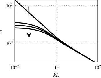
. Figure 1 shows the time scale computed from (2.40) for different Richardson numbers ranging from neutral to stable conditions. It can be seen that the proposed time scale implies a decrease in the evolution time scale for the small wavenumbers, while the large ones (small scales) remain practically unaffected, so that their level of anisotropy remains unchanged by stratification.




For a given dimensionless wavenumber vector,
 $\boldsymbol{k}_{0}=(k_{1,0},\,k_{2,0},\,k_{3,0})$
, Brunt–Väisälä frequency,
 $N$
, and shear,
 ${\it\alpha}$
, the eddy breakup time is determined according to equation (2.40), where
 ${\it\tau}_{M94}$
is first computed from (2.39) with
 $$\begin{eqnarray}k=[k_{1,0}^{2}+k_{2,0}^{2}+(k_{3,0}-{\it\alpha}k_{1,0}{\it\tau}_{M94})^{2}]^{1/2},\end{eqnarray}$$
and assuming a value of
 $K$
and
 $c$
to determine the breakup time.
Besides the scaling quantities
 $U_{s}$
and
 $L$
and the initial spectral tensor parameters
 $Q_{u}$
,
 $Q_{{\it\rho}}/Q_{u}$
and
 $L_{{\it\rho}}/L$
, two other parameters are therefore needed to complete the model by determining the breakup time scale, namely
 $K$
and
 $c$
. Their values will be discussed in § 4.
A relevant point concerns the validity of the RDT approximation in the atmospheric boundary layer. According to the analysis reported by Hanazaki & Hunt (Reference Hanazaki and Hunt2004), in order to neglect the nonlinear terms in both the momentum and temperature transport equations, it is necessary that the Froude number
 $\mathit{Fr}_{L}={\it\sigma}_{w}/(NL)\ll 1$
, with
 ${\it\sigma}_{w}$
indicating the vertical velocity standard deviation. This condition was never met with the available dataset, and
 $\mathit{Fr}_{L}$
ranged between 0.8 and 2.5. On the other hand, even the mean shear time scale,
 ${\it\alpha}^{-1}$
, was comparable to the turbulent time scale,
 $\text{TKE}/{\it\epsilon}$
(with TKE indicating the turbulent kinetic energy), so that
 ${\it\alpha}\text{TKE}/{\it\epsilon}=\mathit{O}(1)$
and RDT equations should not be applicable even in the unstratified case. Nevertheless, the discussion above regarding the possibility to introduce the artificial time scale suggests that the use of RDT equations could still be acceptable to develop a model able to estimate the spectra, although outside of the range of application of RDT.
2.3. Numerical implementation
Once
 ${\it\tau}$
was determined from (2.40), it was used in the
 $\unicode[STIX]{x1D648}$
matrix with an evaluation of the Legendre functions of first and second kind at
 $z_{0}$
and
 $z$
. Since the evaluation of the
 $\unicode[STIX]{x1D648}$
matrix had to be carried out for a large number of wavenumber vectors, a fast evaluation of the Legendre functions was needed. This was achieved by approximating the Legendre equation (2.8) at ordinary and singular points as well as by means of a Wentzel–Kramers–Brillouin (WKB) approximation (Bender & Orszag Reference Bender and Orszag1999) of the Legendre functions in the limit of large
 $-{\it\lambda}\left(1+{\it\lambda}\right)$
. Some details about the resulting formulae are provided in appendix A.
Once the isotropic initial condition (2.35) was determined (via the parameters
 $Q_{u}$
,
 $Q_{{\it\rho}}/Q_{u}$
and
 $L_{{\it\rho}}/L$
), (2.34) was used to determine the spectral tensor, while the final wavenumber vector was given by (2.7). The observed two-point velocity and density spectra were obtained by integrating the spectral tensor at time
 ${\it\tau}$
as
 $$\begin{eqnarray}F_{ij}(k_{1};{\rm\Delta}x_{2},{\rm\Delta}x_{3},{\it\tau})=\int _{\mathbb{R}^{2}}{\it\Phi}_{ij}({\it\tau};\boldsymbol{k})\exp [\text{i}k_{2}{\rm\Delta}x_{2}+\text{i}k_{3}{\rm\Delta}x_{3}]\,\text{d}k_{2}\,\text{d}k_{3},\end{eqnarray}$$
where the integration was performed by discretising each wavenumber component into
 $N_{k}$
elements in the positive and negative directions (including the origin there were
 $2N_{k}+1$
points). The points were logarithmically spaced in the range
 $10^{-3}<k<10^{4}$
. To save some computational time, it can be noted that, for a given set of
 $k_{1,0}$
and
 $k_{3,0}$
, the
 $\unicode[STIX]{x1D648}$
matrix is an even function of
 $k_{2,0}$
, except for the terms
 $F_{u_{2}u_{30}}$
and
 $F_{u_{2}{\it\rho}_{0}}$
which are odd functions of
 $k_{2,0}$
. This allowed a reduction by a factor of 2 of the operations needed for the integrated spectra evaluation.
The
 $N_{k}$
parameter was also changed and it was found that a good compromise between accuracy and computational time was provided already by
 $N_{k}\approx 100$
, where an error of less than 1%, compared with the spectral tensor evaluated with
 $N_{k}=500$
, was observed. The majority of the results shown in the paper have been obtained for
 $N_{k}=150$
, with the exception of the five- and four-parameter optimisations, reported in § 4, where
 $N_{k}=70$
was adopted due to the high computational demands.
3. Measurements
In order to validate the model and to determine the various parameters, field measurements with a 138 m tall meteorological tower located over a forested site were used. The measurement site is situated in a production forest approximately 30 km inland of the Swedish south-eastern coast. The average forest height is approximately
 $h_{c}\approx 20$
m. The tower was placed in the north-west corner of a 200 m by 250 m large clearing, and two wind turbines, located to the south and north-east directions respectively, were placed approximately 200 m from the measurement tower. To minimise the effect of these heterogeneities, only data coming from wind directions between
 $240^{\circ }$
and
 $280^{\circ }$
were used in the present study. More details about the set-up of the measurements and data quality control have been reported by Arnqvist et al. (Reference Arnqvist, Segalini, Dellwik and Bergström2015).
In this study we used data from six Metek sonic anemometers at measurement heights of
 $z=40$
, 59, 80, 98, 120 and 138 m and sampled at 20 Hz to determine the velocity and temperature time series. The mean temperature was measured at
 $z=40$
, 98, 120 and 138 m with independent Risø PT-100 temperature sensors, while the atmospheric pressure was monitored at
 $z=40$
m with a Vaisala PTB100B barometer. The time series were divided into 30 min segments, where horizontal velocity components were locally rotated (so that the mean spanwise velocity was
 $V_{0}=0~\text{m}~\text{s}^{-1}$
), identifying the direction of the local mean wind.
The Brunt–Väisälä frequency was computed as
 $N=(g/{\it\Theta}_{0}\,\text{d}{\it\Theta}/\text{d}z)^{1/2}$
, where
 ${\it\Theta}=T_{0}(P_{0}/P)^{R/c_{p}}$
is the potential temperature,
 $P$
is the local mean static pressure,
 $R$
is the gas constant and
 $c_{p}$
is the specific heat capacity. Since the pressure was only measured at the lowest height, the hydrostatic equation and the gas law were used to determine the pressure at the other measurement levels as
 $$\begin{eqnarray}P(z)=P_{0}\left[\frac{T(z)}{T_{0}}\right]^{-(g/R)\left(\text{d}T/\text{d}z\right)^{-1}}.\end{eqnarray}$$
The velocity shear
 ${\it\alpha}=\text{d}U_{0}/\text{d}z$
was determined for each available height from the mean velocity profile by approximating the differential operator with finite differences. The Richardson number was finally calculated by means of its definition,
 $\mathit{Ri}=N^{2}/{\it\alpha}^{2}$
.
In order to characterise the diabatic stability condition of each 30 min block, the Obukhov length was calculated as
 $$\begin{eqnarray}L_{o}=-\frac{u_{\ast }^{3}{\it\Theta}_{0}}{{\it\kappa}g\overline{w^{\prime }{\it\theta}^{\prime }}},\end{eqnarray}$$
where
 $u_{\ast }=[\overline{u^{\prime }w^{\prime }}^{2}+\overline{v^{\prime }w^{\prime }}^{2}]^{1/4}$
is the friction velocity (computed at the lowest available level above the forest,
 $z=40$
m),
 ${\it\Theta}_{0}$
is the potential temperature at
 $z=40$
m,
 ${\it\kappa}=0.4$
is the von Kármán constant used,
 $g=9.81~\text{m s}^{-2}$
is the gravitational acceleration and
 $\overline{w^{\prime }{\it\theta}^{\prime }}$
is the vertical temperature flux from the sonic anemometer at 40 m.
In order to examine the performance of the spectral model in various conditions, averages of the velocity and temperature spectra were performed by subdividing the data in terms of diabatic stability and velocity classes. Four stability classes were introduced as very stable (
 $L_{o}<100$
m), stable (100 m
 ${<}L_{o}<400$
m), near-neutral stability (400 m
 ${<}L_{o}<1000$
m) and neutral (
 $|L_{o}|>1000$
m). Additionally, velocity bins based on the mean velocity at
 $z=80$
m (with increments of
 $1~\text{m}~\text{s}^{-1}$
) were selected, similarly to Chougule et al. (Reference Chougule, Mann, Segalini and Dellwik2015), to identify possible Reynolds-number effects. The spectra were computed for each 30 min time series belonging to a given class at all the available heights, and the resulting multipoint spectra were averaged within the respective bins. For every velocity and stability class, six heights were available, so that 21 possible height combinations and 10 possible component combinations could be obtained, for a total number of 210 multipoint spectra available.
In order to obtain the density cross-spectra or the velocity–density cross-spectra from the available velocity and temperature fluctuations, the Boussinesq approximation was used, so that
 ${\rm\Delta}{\it\rho}/{\it\rho}_{0}=-{\rm\Delta}T/T_{0}$
.
4. Results
According to § 2, the spectral tensor is defined from the velocity and length scales
 $U_{s}$
and
 $L$
and the parameters
 $Q_{u}$
,
 $Q_{{\it\rho}}/Q_{u}$
,
 $L_{{\it\rho}}/L$
,
 $K$
and
 $c$
. The local streamwise velocity standard deviation was chosen as the velocity scale, so that
 $U_{s}={\it\sigma}_{u}$
in the present work. The parameters
 $Q_{u}$
,
 $Q_{{\it\rho}}/Q_{u}$
,
 $L_{{\it\rho}}/L$
,
 $K$
,
 $c$
and
 $L$
were determined from the minimisation of
 $$\begin{eqnarray}\displaystyle J & = & \displaystyle \mathop{\sum }_{m=1}^{14}\left\{\mathop{\sum }_{i=1}^{3}\left[Q_{u}k_{m}F_{ii}^{(est)}(k_{m};\,0,\,0)-\frac{f_{m}F_{ii}^{(meas)}(\,f_{m};\,0,\,0)}{U_{s}^{2}}\right]^{2}\right.\nonumber\\ \displaystyle & & \displaystyle +\,\left[Q_{u}k_{m}F_{13}^{(est)}(k_{m};\,0,\,0)-\frac{f_{m}\text{Re}(F_{13}^{(meas)}(\,f_{m};\,0,\,0))}{U_{s}^{2}}\right]^{2}\nonumber\\ \displaystyle & & \displaystyle +\,\left.100\left[Q_{u}k_{m}F_{3{\it\rho}}^{(est)}(k_{m};\,0,\,0)+\frac{f_{m}\text{Re}(F_{3{\it\theta}}^{(meas)}(\,f_{m};\,0,\,0))}{U_{s}\,T_{0}\,\mathit{Fr}^{2}}\right]^{2}\right\}.\end{eqnarray}$$
 $k$
was computed from the frequency,
 $f$
, by means of the Taylor hypothesis as
 $k=2{\rm\pi}f/U_{0}$
. The minimisation of (4.1) implies the search for the parameters that provide the least-square deviation (at 14 logarithmically spaced frequencies) between the pre-multiplied single-point spectral densities
 $fF_{uu}$
,
 $fF_{vv}$
,
 $fF_{ww}$
, and co-spectra
 $f\text{Re}(F_{uw})$
and
 $f\text{Re}(F_{w{\it\theta}})$
, while the spectra
 $fF_{uv}$
,
 $fF_{vw}$
and
 $fF_{v{\it\theta}}$
were not compared since they are zero from the model due to symmetry reasons. No requirement was introduced about the agreement between the measured and predicted single-point
 $fF_{u{\it\theta}}$
and all the two-point spectra. Therefore, the comparison of the model with the latter quantities will be the benchmark to assess its quality.
The power spectrum of the temperature was omitted from the comparison and parameter search since the quality of the sonic power temperature spectra was found to be lower than that of the cross-spectra of temperature and velocity. The raw signals of the sonic anemometer were corrected according to Liu, Peters & Foken (Reference Liu, Peters and Foken2001), but still the power spectrum of the temperature showed consistent high-frequency noise. By examining the effect of different filters and corrections on the spectra from sonic temperature measurements, Nielsen & Larsen (Reference Nielsen and Larsen2002) showed that the power spectra of the temperature may be affected by high-frequency noise, while the cross-spectra are almost unaffected, provided that the temperature is derived from several sonic paths (which is done in the algorithms of Liu et al.
Reference Liu, Peters and Foken2001). However, besides the experimental uncertainty at high frequencies, the disagreement between the model and the measurements in the temperature spectrum could also be a result of the model approximations (large
 $\mathit{Fr}_{L}$
, introduction of the artificial time scale
 ${\it\tau}$
, etc.) and only numerical simulations or high-quality experiments will be able to clarify this issue.
As is clear from (4.1), the
 $Q_{u}$
parameter can be found by means of a linear least-square approach, so that, for a given set of parameters
 $L$
,
 $Q_{{\it\rho}}/Q_{u}$
,
 $L_{{\it\rho}}/L$
,
 $K$
and
 $c$
, there exists only one
 $Q_{u}$
that will minimise
 $J$
. The purpose of (4.1) is the identification of the remaining five nonlinear coefficients to reveal their (eventual) dependence on the velocity magnitude and Richardson number. Among the available velocity and stability classes, 156 spectra from the six different heights were available to identify the parameters. Additional measurements over a low-roughness site called Maglarp (Smedman & Bergström Reference Smedman and Bergström1984) were used to provide further support to the obtained parameters and to identify their sensitivity to the surface roughness. However, due to the limited amount of data, the spectra from Maglarp were not averaged over different 30 min segments, so the scatter is expected to be larger. Rather, they were subdivided into 40 windows to reduce the random error, following the guidelines of Bendat & Piersol (Reference Bendat and Piersol1986).
Initially, all five parameters were allowed to vary and the algorithm fminsearch of Matlab was used to identify the local optimum. This allowed identification of the averaged value of
 $L_{{\it\rho}}/L\approx 1$
with a limited amount of scatter. By recognising that the optimisation algorithm performs better and faster in a reduced dimensional search space, the parameter
 $L_{{\it\rho}}/L$
was kept fixed to
 $1$
and a four-parameter optimisation was performed to identify
 $c$
, and so forth. The values of the optimal parameters and the associated averaged error function
 $J$
are reported in table 1 with their respective 95 % confidence intervals. It can be noted that, as already anticipated, the expected
 $L_{{\it\rho}}/L$
is approximately 1, namely the large-scale density-carrying eddies have the same size as the equivalent energy-carrying eddies. Surprisingly, the value of the
 $K$
parameter is systematically higher than the value reported by Mann and co-workers (where
 $K\approx 3$
). A possible explanation for this discrepancy might be that the present objective function
 $J$
, stated by (4.1), is different from the
 ${\it\chi}^{2}$
fit proposed in M94, which is not focused on pre-multiplied spectra but rather on velocity spectra weighted by the statistical (frequency-dependent) random error. Furthermore, the presence of a stratification correction term in (2.40) will reduce the breakup time, virtually reducing the value of
 $K$
if the stratification has not been considered. As a result of the optimisation process, constant values of
 $K\approx 3.78$
and
 $c\approx 0.15$
have been obtained, reducing the number of free parameters of the model. Since
 $c$
was allowed to vary freely in the optimisation scheme, the possibility of
 $c=0$
existed, which would have meant that no effect of stratification on
 ${\it\tau}$
could be seen. The obtained non-zero
 $c$
value indicates that the stratification indeed has an effect in the time scale, opposite to the assumption of Chougule (Reference Chougule2013).
Values of the model parameters after the optimisation process and averaged error
 $J$
. The number of wavenumbers used in each optimisation,
 $N_{k}$
, is also reported.

Apart from the parameters obtained by means of the optimisation routine, the value of
 $Q_{u}$
must be found, as it determines the magnitude of the normalised spectra. By looking at (4.1), it is evident that the optimal
 $Q_{u}$
must ensure a good fit for several spectra. However, it can be expected that the integral of the (normalised) streamwise velocity spectrum should be the same, so that
 $$\begin{eqnarray}Q_{u}\int _{0}^{\infty }F_{uu}^{(est)}(k_{1})\,\text{d}k_{1}\approx 1\longrightarrow Q_{u}\approx \left[\int _{0}^{\infty }F_{uu}^{(est)}(k_{1})\,\text{d}k_{1}\right]^{-1}.\end{eqnarray}$$
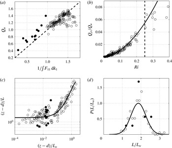
Figure 2 shows the comparison between the observed
 $Q_{u}$
(which accounts for all of the spectra) and the estimated one, providing a reasonable collapse between the data. The second parameter is the relative importance between the initial density and velocity spectra,
 $Q_{{\it\rho}}/Q_{u}$
. In this case a significant Richardson-number dependence is observed and the parameter can be approximated by means of the parabola
 $$\begin{eqnarray}\frac{Q_{{\it\rho}}}{Q_{u}}\approx 0.712\,\mathit{Ri}^{2}+0.04\,\mathit{Ri}.\end{eqnarray}$$
Looking at figure 2(b), the agreement of the points with the proposed fit is also good and the only deviation comes from the highly stable data. The deviation from the curve might be due to the limited amount of data used to compute the averages of the experimental data at such highly stable conditions, but it should be noted that there the Richardson number is greater than 0.25, which corresponds to the critical
 $\mathit{Ri}$
where the linear mechanisms should suppress turbulence (Miles Reference Miles1961), and the stratified RDT equations follow similar dynamics as well.
The characteristic length scale,
 $L$
, follows a scaling similar to the one proposed by Sullivan et al. (Reference Sullivan, Horst, Lenschow, Moeng and Weil2003) for the peak of the pre-multiplied vertical velocity spectrum,
 $L_{w}$
: the ratio
 $(z-d)/L$
seems to be function of the stability parameter
 $(z-d)/L_{o}$
as
 $(z-d)/L_{w}$
does. Clearly, this suggests that the ratio
 $L/L_{w}$
should be constant, and figure 2(d) shows its probability distribution, which is reasonably well approximated by a Gaussian curve. It is noteworthy that both the forested and low-roughness data peak at
 $L/L_{w}\approx 1.9$
.
Parameters of the spectral model: (a)
 $Q_{u}$
as a function of the inverse integral of the estimated streamwise power density spectrum; (b)
 $Q_{{\it\rho}}/Q_{u}$
as a function of the Richardson number (the solid line is (4.3)); (c) scaled length scale
 $L$
as a function of the stability parameter
 $(z-d)/L_{o}$
(the solid line is equation (4.5) of Sullivan et al.
Reference Sullivan, Horst, Lenschow, Moeng and Weil2003, divided by 1.9, namely the averaged
 $L/L_{w}$
); (d) probability density function of the ratio
 $L/L_{w}$
. A Gaussian distribution is plotted for visual aid. The empty circles are Ryningsnäs data while the filled circles are Maglarp data. The vertical dashed line in
 $(b)$
indicates the critical Richardson number,
 $\mathit{Ri}_{c}=0.25$
.

Going back to the parameter
 $Q_{{\it\rho}}/Q_{u}$
, it is interesting to note that such a parameter can be approximately obtained by considering its definition (2.38) and the approximation that the turbulent kinetic energy and density-variance dissipation of the initial field are close to the final ones. That assumption applies when
 ${\it\tau}$
is small, which implies that
 ${\it\alpha}$
or
 $N$
is large. The turbulent kinetic energy dissipation of a stratified medium is given by (Wyngaard Reference Wyngaard2010)
 $$\begin{eqnarray}{\it\epsilon}={\it\nu}\overline{\left(\frac{\partial u_{i}^{\prime }}{\partial x_{j}}\right)^{2}}\approx -\overline{u^{\prime }w^{\prime }}\frac{\text{d}U}{\text{d}z}-\frac{g}{{\it\rho}_{0}}\overline{{\it\rho}^{\prime }w^{\prime }}=-\overline{u^{\prime }w^{\prime }}{\it\alpha}-\frac{g}{{\it\rho}_{0}}\overline{{\it\rho}^{\prime }w^{\prime }},\end{eqnarray}$$
while the dissipation of half of the density variance is provided by
 $$\begin{eqnarray}{\it\epsilon}_{{\it\rho}}={\it\kappa}_{{\it\theta}}\overline{\left(\frac{\partial {\it\rho}^{\prime }}{\partial x_{j}}\right)^{2}}\approx -\overline{{\it\rho}^{\prime }w^{\prime }}\frac{\text{d}{\it\rho}_{0}}{\text{d}z}=\frac{{\it\rho}_{0}}{g}N^{2}\,\overline{{\it\rho}^{\prime }w^{\prime }},\end{eqnarray}$$
where
 ${\it\kappa}_{{\it\theta}}$
is the thermal diffusivity of the fluid.
In stable conditions it is possible to approximate the gradient Richardson number with the flux Richardson number (Kaimal & Finnigan Reference Kaimal and Finnigan1994), leading to
 $$\begin{eqnarray}\mathit{Ri}_{f}=\frac{(g/{\it\rho}_{0})\overline{{\it\rho}^{\prime }w^{\prime }}}{-\overline{u^{\prime }w^{\prime }}{\it\alpha}}\approx \mathit{Ri}=\frac{N^{2}}{{\it\alpha}^{2}}\longrightarrow \frac{g}{{\it\rho}_{0}}\overline{{\it\rho}^{\prime }w^{\prime }}=-\overline{u^{\prime }w^{\prime }}{\it\alpha}\mathit{Ri},\end{eqnarray}$$
so that the dimensionless dissipation ratio is
 $$\begin{eqnarray}\frac{{\it\epsilon}_{{\it\rho}}U_{s}^{2}}{{\it\rho}_{0}^{2}{\it\epsilon}}\approx \mathit{Fr}^{4}\left(\frac{NL}{U_{s}}\right)^{2}\frac{\mathit{Ri}}{1-\mathit{Ri}}\end{eqnarray}$$
and
 $$\begin{eqnarray}\left(\frac{Q_{{\it\rho}}}{Q_{u}}\right)_{\text{est}}\approx \frac{5{\it\beta}_{1}}{6{\rm\pi}{\it\alpha}_{1}}\left(\frac{NL}{U_{s}}\right)^{2}\frac{\mathit{Ri}}{1-\mathit{Ri}}\left(\frac{L_{{\it\rho}}}{L}\right)^{11/3}\approx \frac{5{\it\beta}_{1}}{6{\rm\pi}{\it\alpha}_{1}}\left(\frac{NL}{U_{s}}\right)^{2}\frac{\mathit{Ri}}{1-\mathit{Ri}}.\end{eqnarray}$$
Expression (4.8) provides a simple estimation of the
 $Q_{{\it\rho}}/Q_{u}$
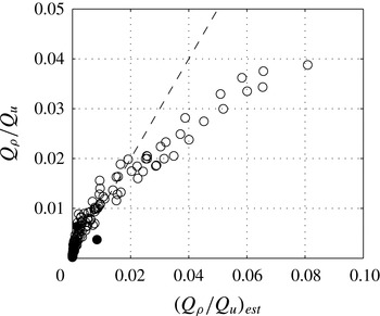
parameter, related to the amplitude of the initial density fluctuation spectrum compared with the velocity one. Figure 3 shows a scatter plot with a comparison between the estimated and calculated parameters. The agreement is fairly good for
 $Q_{{\it\rho}}/Q_{u}<0.02$
(namely for
 $\mathit{Ri}<0.15$
), supporting this simplified estimate.
Comparison between the observed
 $Q_{{\it\rho}}/Q_{u}$
parameter and the one estimated from (4.8). The empty circles are Ryningsnäs data while the filled circles are Maglarp data.

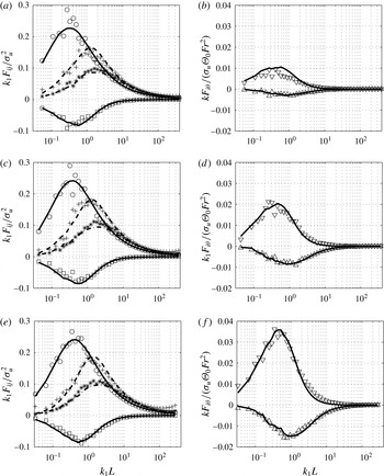
Figure 4 shows the comparison between the single-point spectra,
 $F_{uu}$
,
 $F_{vv}$
,
 $F_{ww}$
,
 $F_{uw}$
,
 $F_{u{\it\theta}}$
and
 $F_{w{\it\theta}}$
, for the velocity bin
 $7~\text{m}~\text{s}^{-1}$
and for three stability classes at
 $z=100$
m. It can be seen that the single-point velocity spectra are well fitted by the present model, and similarly for the
 $F_{w{\it\theta}}$
spectrum. Interestingly, the
 $F_{u{\it\theta}}$
(the only one that was not accounted for in the
 $J$
function in (4.1)) does not agree with the model in the small-wavenumber range for neutral stratification, but it agrees reasonably well already for slightly stable conditions, although with a slightly faster decay than the measurements. For
 $F_{w{\it\theta}}$
both the model and the measurements follow the
 $-7/3$
law in the inertial subrange.
Comparison of the pre-multiplied spectra at
 $z\approx 100~\text{m}$
and
 $U(z)\approx 7~\text{m}~\text{s}^{-1}$
for (a,b) neutral conditions (
 $\mathit{Ri}\approx 0.07$
), (c,d) near-neutral stability conditions (
 $\mathit{Ri}\approx 0.10$
) and (e,f) stable conditions (
 $\mathit{Ri}\approx 0.14$
). Experimental data:
 $(\circ )$
 $F_{uu}$
,
 $(+)$
 $F_{vv}$
,
 $(\ast )$
 $F_{ww}$
, (▫)
 $F_{uw}$
,
 $({\bigtriangledown})$
 $F_{u{\it\theta}}$
,
 $(\triangle )$
 $F_{w{\it\theta}}$
. Model prediction: (solid line)
 $F_{uu}$
,
 $F_{uw}$
,
 $F_{u{\it\theta}}$
,
 $F_{w{\it\theta}}$
; (dashed line)
 $F_{vv}$
; (dash-dotted line)
 $F_{ww}$
. Since the model predicts only real single-point cross-spectra, only the real parts of the cross-spectra are shown.

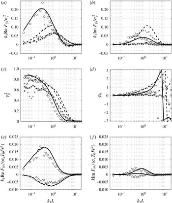
The two-point velocity and temperature cross-spectra are shown in figure 5 for a separation distance of approximately
 ${\rm\Delta}z\approx 20~\text{m}$
. Here, the spectral parameters
 $Q_{u}$
,
 $Q_{{\it\rho}}/Q_{u}$
,
 $U_{s}$
and
 $L$
as well as the mean velocity (to convert the frequency to wavenumber) are averaged between the two heights, as suggested by Chougule et al. (Reference Chougule, Mann, Segalini and Dellwik2015). It is visible that the real part is well predicted (although slightly overestimated), while for the imaginary part there is underestimation in
 $u$
and overestimation in
 $v$
. This has some effect on the coherence, here defined as
 $$\begin{eqnarray}{\it\gamma}_{ij}^{2}=\frac{|F_{ij}(k_{1})|^{2}}{F_{ii}(k_{1})F_{jj}(k_{1})},\end{eqnarray}$$
while little discrepancy is observed in the phase
 ${\it\varphi}$
for small wavenumber where the coherence is high. The fact that the characteristic length scale
 $L$
increases with height
 $z$
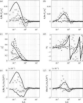
leads to the expectation that the present model will give better results (in terms of two-point cross-spectra) in horizontal planes (see M94) than when a significant vertical separation is present, since the flow is only horizontally homogeneous and new RDT equations should be developed to account for the vertical inhomogeneity. The present model with the present set of parameters seems to lose accuracy at large vertical separation distances, as demonstrated by figure 6, where the two-point spectra are shown for a separation distance of
 ${\rm\Delta}z\approx 60~\text{m}$
(at lower separation distance the agreement is still qualitatively similar to figure 5). The agreement is lost in the real part of the spectrum as well, suggesting that the present model (with the present set of parameters) should be used with caution for
 ${\rm\Delta}z\geqslant 40~\text{m}$
.
Comparison of the pre-multiplied two-point velocity and temperature spectra for
 $z_{1}\approx 80~\text{m}$
,
 $z_{2}\approx 100~\text{m}$
and
 $U(z_{2})\approx 7~\text{m}~\text{s}^{-1}$
for near-neutral stability conditions (
 $\mathit{Ri}\approx 0.10$
). (a) Real part and (b) imaginary part of
 $F_{uu}$
,
 $F_{vv}$
and
 $F_{ww}$
. (c) Coherence and (d) phase functions. (e) Real part and (f) imaginary part of the temperature cross-spectra
 $F_{u{\it\theta}}$
and
 $F_{w{\it\theta}}$
. See figure 4 for the list of symbols.

Comparison of the pre-multiplied two-point velocity and temperature spectra for
 $z_{1}\approx 40~\text{m}$
,
 $z_{2}\approx 100~\text{m}$
and
 $U(z_{2})\approx 7~\text{m}~\text{s}^{-1}$
for near-neutral stability conditions (
 $\mathit{Ri}\approx 0.10$
). (a) Real part and (b) imaginary part of
 $F_{uu}$
,
 $F_{vv}$
and
 $F_{ww}$
. (c) Coherence and (d) phase functions. (e) Real part and (f) imaginary part of the temperature cross-spectra
 $F_{u{\it\theta}}$
and
 $F_{w{\it\theta}}$
. See figure 4 for the list of symbols.

5. Conclusions
In the present paper an analytical solution of the rapid distortion equations is proposed for a homogeneous turbulent flow subjected to uniform shear and stable stratification. The solution allows determination of the timewise evolution of the Fourier transform of the velocity and density fluctuations starting from an arbitrary initial state, as long as the RDT closure is valid. By following the same approach as Mann (Reference Mann1994), a spectral model is proposed based on the stratified RDT solution, where the time-dependent spectral tensor is calculated at a wavenumber-dependent eddy breakup time scale, where it is assumed that at such a time scale the state described by the RDT equations is close to the one observed in the atmosphere.
The model is a function of a number of scaling quantities (the streamwise velocity variance,
 ${\it\sigma}_{u}^{2}$
, and the momentum-carrying large-eddy size,
 $L$
) and parameters (the dimensionless dissipation (to the power 2/3),
 $Q_{u}$
, the ratio between the initial density-variance dissipation and turbulent kinetic energy dissipation,
 $Q_{{\it\rho}}/Q_{u}$
, the ratio between the density- and energy-carrying eddy sizes,
 $L_{{\it\rho}}/L$
, and two additional parameters related to the breakup time, namely
 $K$
and
 $c$
, related to the original Mann model time scale and its sensitivity to the stratification respectively). These have all been determined by optimising the comparison with measurements over a forested area (Arnqvist et al.
Reference Arnqvist, Segalini, Dellwik and Bergström2015) and further supported by low-roughness data (Smedman & Bergström Reference Smedman and Bergström1984). The availability of these two datasets allowed the determination of the parameters, providing some rationale about them in terms of the Richardson number.
The model parameter
 $L$
was shown to scale with the similarity function proposed by Sullivan et al. (Reference Sullivan, Horst, Lenschow, Moeng and Weil2003), originally proposed for the peak of the vertical velocity spectrum
 $L_{w}$
, suggesting that
 $L/L_{w}$
is approximately constant (here found to be approximately 1.9). Since
 $L_{w}$
increases with height,
 $L$
changes with
 $z$
accordingly, an issue that could be included in the analysis to extend the model and to improve the two-point cross-spectra evaluation with significant vertical separation.
The proposed model is able to determine reasonably well the single-point velocity spectra and the velocity and temperature cross-spectra (including
 $F_{u{\it\theta}}$
which was purposefully kept out of the optimisation approach) for different Richardson numbers. When evaluated against vertically separated two-point spectra, the model showed promising results for the phase lag and the co-spectra, but a positive bias was found for the coherence.
In order to test the model predictions of single-point temperature spectra against measurements of high quality, the model was compared with single-point temperature spectra and with estimations provided by Kaimal et al. (Reference Kaimal, Wyngaard, Izumi and Coté1972), showing little agreement at neutral conditions and increasing agreement as
 $\mathit{Ri}$
increased. The model and measurements agreed only for very stable data, despite the fact that the temperature–velocity cross-spectra agree also for lower Richardson numbers. This implies that the present parameters
 $Q_{{\it\rho}}/Q_{u}$
,
 $L_{{\it\rho}}/L$
and
 $c$
may not correspond to the ones that ensure agreement between both velocity and temperature spectra and cross-spectra. Other possible causes of this discrepancy might be the use of the artificial time scale
 ${\it\tau}(k)$
or the fact that RDT equations are not strictly applicable to the present atmospheric boundary layer dataset, according to the scaling argument proposed by Hanazaki & Hunt (Reference Hanazaki and Hunt2004). Further studies comparing the modelled temperature power spectra with high-quality measurements are needed to examine the cause of the discrepancy in near-neutral stratification.
Acknowledgements
This work was supported by the Swedish strategic research programmes STandUP for Wind and Vindforsk IV. The authors wish to thank Professor J. Mann, Dr M. Kelly, Dr G. Brethouwer and Dr A. Chougule for the fruitful discussions. The authors would also like to thank Dr H. Bergström for providing the Maglarp data. I. Carlén is greatly acknowledged for encouraging this work.
Appendix A. Series expansions of the Legendre functions
The Legendre equation
 $$\begin{eqnarray}(1-z^{2})\frac{\text{d}^{2}y}{\text{d}z^{2}}-2z\frac{\text{d}y}{\text{d}z}+{\it\lambda}(1+{\it\lambda})y=0,\end{eqnarray}$$
has three regular singular points at
 $z=\pm 1$
and
 $z=\infty$
. For any ordinary point
 $z_{0}$
, a Taylor series can be assumed of the form
 $$\begin{eqnarray}y=\mathop{\sum }_{n=0}^{\infty }a_{n}(z-z_{0})^{n},\end{eqnarray}$$
where the coefficients
 $a_{n}$
satisfy the recurrence relationship
 $$\begin{eqnarray}a_{n+2}=\frac{2z_{0}(n+1)}{(1-z_{0}^{2})(n+2)}a_{n+1}+\frac{n^{2}+n-{\it\lambda}(1+{\it\lambda})}{(1-z_{0}^{2})(n+1)(n+2)}a_{n}.\end{eqnarray}$$
There are two parameters in (A 3), namely
 $a_{0}$
and
 $a_{1}$
, representing the value of the solution and its derivative at
 $z=z_{0}$
. With the two parameters, two independent solutions of (A 1) can be obtained with
 $$\begin{eqnarray}a_{0}=_{2}F_{1}\left(-{\it\lambda},{\it\lambda}+1;1;\frac{1-z_{0}}{2}\right),\end{eqnarray}$$
 $$\begin{eqnarray}a_{1}=\frac{1}{2}{\it\lambda}({\it\lambda}+1)_{2}F_{1}\left(-{\it\lambda}+1,{\it\lambda}+2;2;\frac{1-z_{0}}{2}\right)\end{eqnarray}$$
for
 $P_{{\it\lambda}}(z)$
and
 $$\begin{eqnarray}\displaystyle a_{0} & = & \displaystyle K_{1}\,z\,_{2}F_{1}\left(\frac{1-{\it\lambda}}{2},\frac{{\it\lambda}}{2}+1;\frac{3}{2};z_{0}^{2}\right)-K_{2}\,_{2}F_{1}\left(-\frac{{\it\lambda}}{2},\frac{{\it\lambda}+1}{2};\frac{1}{2};z_{0}^{2}\right),\end{eqnarray}$$
 $$\begin{eqnarray}\displaystyle a_{1} & = & \displaystyle K_{1}\,\text{}_{2}F_{1}\left(\frac{1-{\it\lambda}}{2},\frac{{\it\lambda}}{2}+1;\frac{3}{2};z_{0}^{2}\right)\nonumber\\ \displaystyle & & \displaystyle +\,\frac{\left(1-{\it\lambda}\right)\left({\it\lambda}+2\right)}{3}K_{1}\,z^{2}\,\text{}_{2}F_{1}\left(\frac{3-{\it\lambda}}{2},\frac{{\it\lambda}}{2}+2;\frac{5}{2};z_{0}^{2}\right)\nonumber\\ \displaystyle & & \displaystyle +\,{\it\lambda}({\it\lambda}+1)K_{2}\,z\,_{2}F_{1}\left(1-\frac{{\it\lambda}}{2},\frac{{\it\lambda}+3}{2};\frac{3}{2};z_{0}^{2}\right)\end{eqnarray}$$
 $Q_{{\it\lambda}}(z)$
, with
 $$\begin{eqnarray}K_{1}=\frac{\sqrt{{\rm\pi}}\cos \left({\displaystyle \frac{{\rm\pi}{\it\lambda}}{2}}\right){\it\Gamma}\left(1+{\displaystyle \frac{{\it\lambda}}{2}}\right)}{{\it\Gamma}\left({\displaystyle \frac{1+{\it\lambda}}{2}}\right)},\quad K_{2}=\frac{\sqrt{{\rm\pi}}\sin \left({\displaystyle \frac{{\rm\pi}{\it\lambda}}{2}}\right){\it\Gamma}\left({\displaystyle \frac{1+{\it\lambda}}{2}}\right)}{2{\it\Gamma}\left(1+{\displaystyle \frac{{\it\lambda}}{2}}\right)},\end{eqnarray}$$
where
 ${\it\Gamma}$
is the gamma function (Abramowitz & Stegun Reference Abramowitz and Stegun1964).
Since in the present work
 $z$
belongs to the imaginary axis, the only regular singular point of interest is
 $z=\text{i}\infty$
. By introducing the transformation
 $x=1/z$
, (A 1) becomes
 $$\begin{eqnarray}(x^{4}-x^{2})\frac{\text{d}^{2}y}{\text{d}x^{2}}+2x^{3}\frac{\text{d}y}{\text{d}x}+{\it\lambda}(1+{\it\lambda})y=0.\end{eqnarray}$$
Since
 $x=0$
is a regular singular point for (A 9), a Frobenius series can be used as
 $$\begin{eqnarray}y=x^{{\it\alpha}}\mathop{\sum }_{n=0}^{\infty }b_{n}x^{n}=z^{-{\it\alpha}}\mathop{\sum }_{n=0}^{\infty }\frac{b_{n}}{z^{n}},\end{eqnarray}$$
where the exponent
 ${\it\alpha}$
is a root of the characteristic polynomial
 $P({\it\alpha})={\it\alpha}({\it\alpha}-1)-{\it\lambda}({\it\lambda}+1)$
. Two solutions are indeed possible (
 $y_{1}(z)$
with
 ${\it\alpha}_{1}=-{\it\lambda}$
and
 $y_{2}(z)$
with
 ${\it\alpha}_{2}={\it\lambda}+1$
), corresponding to a linear combination of the two Legendre functions. The even coefficients
 $b_{n}$
satisfy the general recursive relationship
 $$\begin{eqnarray}b_{n+2}=\frac{(n+{\it\alpha})(n+{\it\alpha}+1)}{(n+{\it\alpha}+1)(n+{\it\alpha}+2)-{\it\lambda}({\it\lambda}+1)}b_{n},\end{eqnarray}$$
with
 $b_{0}=1$
while the odd coefficients are 0. This allows the construction of two linearly independent solutions of (A 1), named
 $y_{1}$
and
 $y_{2}$
, linearly related to the Legendre functions. As
 $z\rightarrow \infty$
, and for
 ${\it\lambda}\neq -1/2$
, the Legendre functions behave as
 $$\begin{eqnarray}\displaystyle & \displaystyle P_{{\it\lambda}}(z)=\frac{2^{{\it\lambda}+1}{\it\Gamma}(-2{\it\lambda}-1)}{{\it\Gamma}^{2}(-{\it\lambda})}z^{-({\it\lambda}+1)}+\frac{{\it\Gamma}(2{\it\lambda}+1)}{2^{{\it\lambda}}{\it\Gamma}^{2}({\it\lambda}+1)}z^{{\it\lambda}}, & \displaystyle\end{eqnarray}$$
 $$\begin{eqnarray}\displaystyle & \displaystyle Q_{{\it\lambda}}(z)=c_{1}z^{-({\it\lambda}+1)}+c_{2}z^{{\it\lambda}}, & \displaystyle\end{eqnarray}$$
 $$\begin{eqnarray}\displaystyle & \displaystyle c_{1}=\sqrt{{\rm\pi}}{\it\Gamma}\left(-\frac{1}{2}-{\it\lambda}\right)\text{i}^{\pm ({\it\lambda}+1)}\left[\frac{K_{1}\text{i}^{\pm 1}}{2{\it\Gamma}^{2}\left({\displaystyle \frac{1-{\it\lambda}}{2}}\right)}-{\displaystyle \frac{K_{2}}{{\it\Gamma}^{2}\left(-{\displaystyle \frac{{\it\lambda}}{2}}\right)}}\right], & \displaystyle\end{eqnarray}$$
 $$\begin{eqnarray}\displaystyle & \displaystyle c_{2}=\sqrt{{\rm\pi}}{\it\Gamma}\left({\displaystyle \frac{1}{2}}+{\it\lambda}\right)\text{i}^{\mp {\it\lambda}}\left[{\displaystyle \frac{K_{1}\text{i}^{\pm 1}}{2{\it\Gamma}^{2}\left(1+{\displaystyle \frac{{\it\lambda}}{2}}\right)}}-{\displaystyle \frac{K_{2}}{{\it\Gamma}^{2}\left({\displaystyle \frac{{\it\lambda}+1}{2}}\right)}}\right] & \displaystyle\end{eqnarray}$$
 $\pm$
depends on the sign of the imaginary part of
 $z$
. The Legendre functions can therefore be expressed as
 $$\begin{eqnarray}\displaystyle & \displaystyle P_{{\it\lambda}}(z)=\frac{2^{{\it\lambda}+1}{\it\Gamma}(-2{\it\lambda}-1)}{{\it\Gamma}^{2}(-{\it\lambda})}y_{1}(z)+\frac{{\it\Gamma}(2{\it\lambda}+1)}{2^{{\it\lambda}}{\it\Gamma}^{2}({\it\lambda}+1)}y_{2}(z), & \displaystyle\end{eqnarray}$$
 $$\begin{eqnarray}\displaystyle & \displaystyle Q_{{\it\lambda}}(z)=c_{1}y_{1}(z)+c_{2}y_{2}(z). & \displaystyle\end{eqnarray}$$
In the special case of
 ${\it\lambda}=-1/2$
,
 ${\it\alpha}_{1}={\it\alpha}_{2}=1/2$
and only one solution can be expressed as (A 10) (say
 $y_{1}$
), while the other can be expressed as (Bender & Orszag Reference Bender and Orszag1999)
 $$\begin{eqnarray}y_{2}=-\frac{\ln z}{\sqrt{z}}\mathop{\sum }_{n=0}^{\infty }\frac{b_{n}}{z^{n}}+\frac{1}{\sqrt{z}}\mathop{\sum }_{n=0}^{\infty }\left(\frac{\partial b_{n}}{\partial {\it\alpha}}\right)_{{\it\alpha}=1/2}z^{-n},\end{eqnarray}$$
with
 $$\begin{eqnarray}\frac{\partial b_{n+2}}{\partial {\it\alpha}}=\frac{4n+5}{2(n+2)^{3}}b_{n}+\frac{(2n+1)(2n+3)}{4(n+2)^{2}}\frac{\partial b_{n}}{\partial {\it\alpha}}\end{eqnarray}$$
and
 $\partial b_{0}/\partial {\it\alpha}=0$
. Consequently,
 $P_{-1/2}(z)$
is given by
 $$\begin{eqnarray}P_{-1/2}(z)=\frac{3\sqrt{2}\ln 2}{{\rm\pi}}y_{1}(z)-\frac{\sqrt{2}}{{\rm\pi}}y_{2}(z),\end{eqnarray}$$
while
 $Q_{-1/2}(z)$
is given by
 $$\begin{eqnarray}\displaystyle Q_{-1/2}(z) & = & \displaystyle \sqrt{{\rm\pi}}\left[\frac{K_{1}}{{\it\Gamma}^{2}(3/4)}\text{i}^{\pm 3/2}\left(\mp \text{i}\frac{{\rm\pi}}{2}-{\it\gamma}-{\it\psi}\left(\frac{3}{4}\right)\right)\right.\nonumber\\ \displaystyle & & \displaystyle \left.-\,\frac{2K_{2}}{{\it\Gamma}^{2}(1/4)}\text{i}^{\pm 1/2}\left(\mp \text{i}\frac{{\rm\pi}}{2}-{\it\gamma}-{\it\psi}\left(\frac{1}{4}\right)\right)\right]y_{1}(z)\nonumber\\ \displaystyle & & \displaystyle -\,\sqrt{{\rm\pi}}\left[\frac{K_{1}}{{\it\Gamma}^{2}(3/4)}\text{i}^{\pm 3/2}-\frac{2K_{2}}{{\it\Gamma}^{2}(1/4)}\text{i}^{\pm 1/2}\right]y_{2}(z),\end{eqnarray}$$
 ${\it\psi}$
is the digamma function (Abramowitz & Stegun Reference Abramowitz and Stegun1964).
If
 $(Nk_{h}/({\it\alpha}k_{1}))^{2}=-{\it\lambda}(1+{\it\lambda})\gg 1$
the Legendre functions become rapidly oscillating and the regular point expansions become increasingly inaccurate. A WKB approximation (Bender & Orszag Reference Bender and Orszag1999) is therefore pursued based on the small parameter
 ${\it\epsilon}=[-{\it\lambda}(1+{\it\lambda})]^{-1/2}$
for (A 1) rewritten as
 $$\begin{eqnarray}{\it\epsilon}^{2}\left[(1-z^{2})\frac{\text{d}^{2}y}{\text{d}z^{2}}-2z\frac{\text{d}y}{\text{d}z}\right]-y=0.\end{eqnarray}$$
As usual in the WKB approach, the solution
 $y(z)$
is assumed to be of the form
 $$\begin{eqnarray}y(z)\sim \exp \left[\frac{1}{{\it\epsilon}}S_{0}(z)+S_{1}(z)+{\it\epsilon}S_{2}(z)+{\it\epsilon}^{2}S_{3}(z)+\mathit{O}({\it\epsilon}^{3})\right].\end{eqnarray}$$
By substituting the ansatz (A 23) into (A 22), it is possible to obtain the expressions for the unknown functions
 $S_{n}$
as
 $$\begin{eqnarray}\displaystyle & \displaystyle S_{0}(z)=\pm \arcsin (z), & \displaystyle\end{eqnarray}$$
 $$\begin{eqnarray}\displaystyle & \displaystyle S_{1}(z)=-{\textstyle \frac{1}{4}}\ln (1-z^{2}), & \displaystyle\end{eqnarray}$$
 $$\begin{eqnarray}\displaystyle & \displaystyle S_{2}(z)=\mp \frac{1}{8}\left[\frac{z}{\sqrt{1-z^{2}}}+\arcsin (z)\right], & \displaystyle\end{eqnarray}$$
 $$\begin{eqnarray}\displaystyle & \displaystyle S_{3}(z)=\frac{1}{16(1-z^{2})}. & \displaystyle\end{eqnarray}$$
As
 ${\it\epsilon}\rightarrow 0$
the Legendre functions can therefore be approximated as
 $P_{{\it\lambda}}(z)\approx c_{+}y_{+}(z)+c_{-}y_{-}(z)$
(and similarly for
 $Q_{{\it\lambda}}(z)$
), where the functions
 $y_{+}(z)$
and
 $y_{-}(z)$
are
 $$\begin{eqnarray}\displaystyle & \displaystyle y_{+}(z)=\frac{1}{(1-z^{2})^{1/4}}\exp \left[\frac{\arcsin (z)}{{\it\epsilon}}-\frac{{\it\epsilon}}{8}\left(\frac{z}{\sqrt{1-z^{2}}}+\arcsin (z)\right)+\frac{{\it\epsilon}^{2}}{16(1-z^{2})}\right], & \displaystyle \nonumber\\ \displaystyle & & \displaystyle\end{eqnarray}$$
 $$\begin{eqnarray}\displaystyle & \displaystyle y_{-}(z)=\frac{1}{(1-z^{2})^{1/4}}\exp \left[-\frac{\arcsin (z)}{{\it\epsilon}}+\frac{{\it\epsilon}}{8}\left(\frac{z}{\sqrt{1-z^{2}}}+\arcsin (z)\right)+\frac{{\it\epsilon}^{2}}{16(1-z^{2})}\right] & \displaystyle \nonumber\\ \displaystyle & & \displaystyle\end{eqnarray}$$
 $c_{+}$
and
 $c_{-}$
are obtained from the knowledge of the Legendre function value and derivative at a certain point (
 $z=0$
in the present implementation).