1. Introduction
The injection of fluid into the narrow liquid-filled gap between a rigid plate and an elastic membrane drives a displacement flow that is controlled by the competition between elastic and viscous forces. If the membrane is very stiff, the fluid advances primarily into the gap whose width remains approximately constant; if the membrane is very flexible, the injected fluid is accommodated mainly by the inflation of the membrane in the vicinity of the injection point. The problem involves a two-way interaction between fluid and solid mechanics, and may be affected by additional physical effects, such as gravity or (in the case of the injection of a different immiscible fluid) interfacial tension.
Elastohydrodynamic interactions of this type arise in applications ranging from geophysical phenomena such as the formation of laccoliths (Michaut Reference Michaut2011; Lister, Peng & Neufeld Reference Lister, Peng and Neufeld2013) and gravity-driven surface lava flows under solidified crusts (Slim et al. Reference Slim, Balmforth, Craster and Miller2009; Hewitt, Balmforth & de Bruyn Reference Hewitt, Balmforth and de Bruyn2015) to physiological processes. For instance, the formation and growth of blisters (Chopin, Vella & Boudaoud Reference Chopin, Vella and Boudaoud2008) involves a competition between elastic and adhesive forces. The mechanics of pulmonary airway reopening (the process by which liquid-filled collapsed pulmonary airways are reopened by a propagating air finger) is governed by an interaction between viscous, capillary and elastic forces within the more complex geometry of a network of elastic tubes. Early experimental studies of this problem (Perun & Gaver III Reference Perun and Gaver III1985, Reference Perun and Gaver III1995; Gaver III, Samsel & Solway Reference Gaver III, Samsel and Solway1990) indicated that a minimum (yield-) pressure is required to initiate the motion of the air finger. Subsequent two-dimensional (Gaver III et al. Reference Gaver III, Halpern, Jensen and Grotberg1996; Heil Reference Heil2000; Jensen et al. Reference Jensen, Horsburgh, Halpern and Gaver2002) and three-dimensional (Hazel & Heil Reference Hazel and Heil2003, Reference Hazel and Heil2005) theoretical/computational studies showed that the relationship between the driving pressure and the steady propagation speed of the air finger has a minimum which separates two distinct flow regimes. At high speeds, the air finger ‘peels’ the collapsed airway walls apart, while at low speeds, the air finger ‘pushes’ a large volume of fluid ahead of its tip. The temporal stability of these solutions was studied (in the two-dimension setting) by Halpern et al. (Reference Halpern, Naire, Jensen and Gaver2005), while further flow regimes were identified in experimental studies by Juel & Heap (Reference Juel and Heap2007) and Heap & Juel (Reference Heap and Juel2008). We refer to Heil & Hazel (Reference Heil and Hazel2011) for a recent review.
The current study is motivated by recent work on the injection of an air bubble into an elastic-walled liquid-filled Hele-Shaw cell. These studies showed that the well-known fingering instability that occurs when a gas displaces a viscous fluid in a rigid cell (Saffman & Taylor Reference Saffman and Taylor1958; Paterson Reference Paterson1981; Homsy Reference Homsy1987; Chen Reference Chen1989; Thomé et al. Reference Thomé, Rabaud, Hakim and Couder1989; Miranda & Widom Reference Miranda and Widom1998) can be delayed or even suppressed through changes in cell geometry due to elastohydrodynamic interactions (Pihler-Puzović et al. Reference Pihler-Puzović, Illien, Heil and Juel2012, Reference Pihler-Puzović, Périllat, Russell, Juel and Heil2013; Al-Housseiny, Christov & Stone Reference Al-Housseiny, Christov and Stone2013). Related fluid–structure interaction problems include the peeling of lubricated flexible sheets from viscous substrates (McEwan & Taylor Reference McEwan and Taylor1966; Hosoi & Mahadevan Reference Hosoi and Mahadevan2004) and suppression of ribbing instabilities by the use of elastomer-coated rolls; see, e.g., Carvalho & Scriven (Reference Carvalho and Scriven1997, Reference Carvalho and Scriven1999).
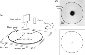
In the present paper we study the canonical problem shown schematically in figure 1 (see also the sketch in figure 3 below), which has received much attention in recent years (Michaut Reference Michaut2011; Pihler-Puzović et al. Reference Pihler-Puzović, Illien, Heil and Juel2012, Reference Pihler-Puzović, Périllat, Russell, Juel and Heil2013; Al-Housseiny et al. Reference Al-Housseiny, Christov and Stone2013; Lister et al. Reference Lister, Peng and Neufeld2013; Hewitt et al. Reference Hewitt, Balmforth and de Bruyn2015). A thin uniform layer of viscous fluid is contained between a rigid plate and an elastic membrane which forms the upper boundary of the cell. Viscous fluid or gas is then injected at a constant flow rate through a central hole in the bottom plate. The injected fluid spreads radially while inflating the sheet. Experiments show that this process occurs via the outward propagation of an approximately axisymmetric front beyond which the sheet remains approximately undeformed and the fluid is at rest.
Experimental and asymptotic studies of single-phase displacement flows in this system indicate that the propagation speed of the front is controlled by the local dynamics in the so-called ‘peeling region’ – the region near the front where the thickness of the fluid layer approaches its initial value (Lister et al. Reference Lister, Peng and Neufeld2013; Hewitt et al. Reference Hewitt, Balmforth and de Bruyn2015). The radial velocity of the front is determined by the interaction between viscous and elastic forces, and therefore depends on which of the elastic restoring forces acting in the membrane is dominant. If the deflection of the sheet is small (relative to its thickness), its stiffness is dominated by bending stresses, whereas for larger deflections, self-induced in-plane stresses become dominant in the central blister. However, even in that case the peeling process can still be predominantly driven locally ‘by bending’ if the sheet is thicker than the initial fluid layer (Lister et al. Reference Lister, Peng and Neufeld2013).
(a) Schematic diagram of the experimental apparatus. (b) Top view of the instantaneous interfacial pattern in the elastic-walled Hele-Shaw cell with a latex membrane in which an air bubble, injected at
 $\dot{V}=50~\text{ml}~\text{min}^{-1}$
, displaces silicone oil. (c) The corresponding shape of the air–liquid interface determined by our image analysis procedure.

If the injected fluid is a gas, the position of the propagating front can be affected by the position of the interface between the two fluids. Surface tension acting at this interface contributes to the force balance at the peeling front and therefore potentially changes the spreading dynamics. Furthermore, as mentioned above, the gas–liquid interface can become unstable to non-axisymmetric fingering instabilities when the injection flow rate exceeds a certain threshold. Pihler-Puzović et al. (Reference Pihler-Puzović, Illien, Heil and Juel2012) were the first to study this two-phase flow problem experimentally. They measured the evolution of the position of the gas–liquid interface and studied the onset of the non-axisymmetric instabilities. Al-Housseiny et al. (Reference Al-Housseiny, Christov and Stone2013) and Lister et al. (Reference Lister, Peng and Neufeld2013) subsequently developed theoretical models of axisymmetric spreading for this experimental system. Both studies described the fluid mechanics by lubrication theory and neglected the effects of gravity and capillary forces at the air–liquid interface. The studies differed in their assumptions about the membrane behaviour and about the role of the interface: Al-Housseiny et al. (Reference Al-Housseiny, Christov and Stone2013) assumed that the membrane stiffness is dominated by bending effects and that the presence of the air–liquid interface affects the propagation dynamics; Lister et al. (Reference Lister, Peng and Neufeld2013) argued that the elastic restoring forces in the membrane are dominated by self-induced tension and that the interface only plays a minor role. Both studies found that their theoretical predictions for the evolution of the bubble radius agreed very well with Pihler-Puzović et al.’s (Reference Pihler-Puzović, Illien, Heil and Juel2012) experimental measurements. Therefore, it is not clear from this comparison alone which of the two models is based on the correct physical assumptions.
The purpose of the present paper is to provide a much more detailed study of axisymmetric single- and two-phase flows in elastic-walled Hele-Shaw cells, using a combination of experiments and computations. We develop a complete theoretical model that is based on the coupled solution of the axisymmetric free-surface Navier–Stokes equations (including the effect of interfacial tension and gravity), and the Föppl–von Kármán equations – a system of equations that is capable of describing the deformation of thin elastic membranes in the bending- and tension-dominated regimes. We perform detailed direct comparisons between the computational results and experimental measurements, and then use the computations to identify the dominant mechanisms involved in the interaction between fluid and solid mechanics. We also contrast our results for single- and two-phase spreading with predictions from a simple lubrication-theory-based fluid model that formed the basis of most previous theoretical studies.
In Part 2 of this work (Peng et al. Reference Peng, Pihler-Puzović, Juel, Heil and Lister2015), we focus more specifically on the role of interfacial tension and the capillary meniscus in the two-phase spreading problem. Using insight gained from the experiments and computations in the present paper, the simple lubrication model is developed to include wetting behaviour, and the corrected predictions give excellent agreement with experiments and computations. The model is then used as the basis for the development of detailed asymptotic analyses of the coupling between the meniscus, the fluid wedge ahead of the meniscus and the dynamics of the peeling region.
This paper is organised as follows. We start by describing the experimental set-up in § 2 and then introduce the theoretical/computational models in § 3. Results are presented in § 4, where we start by demonstrating in § 4.1 that the Föppl–von Kármán equations provide an excellent description of the membrane deformation over the range of deflections encountered in the fluid–structure interaction experiments. In § 4.2, we provide a detailed analysis of the flow fields and membrane deformations in the two-phase fluid–structure interaction problem and demonstrate excellent agreement between the numerical and experimental results. In § 4.2.2, we analyse the temporal evolution of the system in terms of the deflection of the membrane and the radius of the propagating front, and relate these to the scaling laws predicted by previous theoretical models. We also highlight important differences between the single- and two-phase flows and show that, for the parameter regime considered in our experiments, gravity plays an important role in the former problem.
2. Experiments
A schematic diagram of the experimental set-up is shown in figure 1(a). A
 $15$
mm thick float-glass plate, which was accurately levelled to within
 $0.1^{\circ }$
, formed the rigid bottom boundary of the cell. A brass cylinder with a diameter of 19 mm, which appears as the central black circle in figure 1(b), was drilled with an inlet hole of radius
 $R_{inlet}=1.14$
mm and mounted flush at the centre of the float-glass plate to enable the injection of fluids. Elastic sheets of size
 $400~\text{mm}\times 400~\text{mm}$
, made from different materials, were used to form the upper boundary of the cell. We used latex sheets (Supatex) of thickness
 $d=0.34\pm 0.01$
mm and Poisson’s ratio
 ${\it\nu}=0.5$
, and polypropylene films (Film Products Ltd) of thickness
 $d=0.030\pm 0.001$
mm, for which a Poisson’s ratio of
 ${\it\nu}=0.44$
was measured using extensometry. The Young’s modulus,
 $E$
, of the materials was determined by matching experiments and numerical simulations for the inflation of the elastic sheet by a spatially uniform pressure; see § 4.1 for details. The top and bottom boundaries of the cell were separated by a spacer of thickness
 $h_{0}=0.56\pm 0.01$
mm with a circular cutout of radius
 $R_{cell}=18$
cm.
All experiments were performed in a temperature-controlled laboratory at
 $20\pm 1\,^{\circ }\text{C}$
. Prior to each experiment, viscous fluid was injected into the cell until the fluid occupied a circular region of radius
 $R_{outer}<R_{cell}$
, thus leaving an air gap between the fluid and the outer edge of the cell. During the experiments, the air in that gap was able to escape freely through the unsealed sidewalls of the cell. While filling the cell, a heavy glass plate was placed on top of the elastic sheet to suppress any vertical displacement of the membrane. This ensured that the experiments were started from a configuration in which the cell had a uniform depth,
 $h_{0}$
, set by the thickness of the spacer separating the top and bottom boundaries. We confirmed that changes to the initial outer radius of the viscous fluid layer,
 $R_{outer}$
, from 15 to 17 cm had no effect on the results.
The experiments with latex sheets were performed with silicone oil (Basildon Chemicals Ltd; viscosity
 ${\it\mu}=0.9624~\text{kg}~\text{m}^{-1}~\text{s}^{-1}$
, density
 ${\it\rho}=961~\text{kg}~\text{m}^{-3}$
and surface tension
 ${\it\gamma}=0.021~\text{N}~\text{m}^{-1}$
), which wets both glass and latex surfaces. When performing experiments with polypropylene sheets, significant electrostatic forces developed and resulted in an erratic distortion of the air–liquid interface when silicone oil (an electrical insulator) was used as the working fluid. We therefore performed these experiments with a mixture of glycerol and water, whose conductive properties prevented the buildup of electric charges. A mixture containing 10 % purified water by volume (resulting in a fluid with viscosity
 ${\it\mu}=0.305~\text{kg}~\text{m}^{-1}~\text{s}^{-1}$
, density
 ${\it\rho}=1235.1~\text{kg}~\text{m}^{-3}$
and surface tension
 ${\it\gamma}=0.065~\text{N}~\text{m}^{-1}$
) was used. While this mixture only partially wetted the polypropylene sheet (we measured a static contact angle of
 ${\it\theta}=78\pm 5^{\circ }$
), the expanding bubble deposited a continuous film of viscous fluid on the cell boundaries, and dewetting was only observed on time scales longer than that of a typical experiment.
For single-phase experiments, which were performed with the latex membrane only, silicone oil was injected with a KD Scientific syringe pump (KDS120) at constant volumetric flow rates in the range
 $\dot{V}=0.5{-}10~\text{ml}~\text{min}^{-1}$
. The peak flow rate was set by the maximum power of the syringe pump.
For the two-phase experiments, a small circular air bubble of radius
 $R_{init}\approx 5$
mm was injected into the viscous fluid layer through the inlet and allowed to relax before starting the experiment by injecting nitrogen from a compressed gas cylinder. The flow rate was regulated manually by a fine needle valve in the range
 $\dot{V}=50{-}300~\text{ml}~\text{min}^{-1}$
. We monitored
 $\dot{V}$
throughout the experiment using a mass airflow meter (Red-Y Smart Meter PCU1000, Icenta Controls Ltd) and found it to remain constant to within 0.5 % of the set value. The maximum and minimum flow rates in these experiments were set by the susceptibility of the system to non-axisymmetric instabilities. For
 $\dot{V}>300~\text{ml}~\text{min}^{-1}$
, the system was found to be unstable to non-axisymmetric fingering instabilities studied earlier by Pihler-Puzović et al. (Reference Pihler-Puzović, Illien, Heil and Juel2012, Reference Pihler-Puzović, Périllat, Russell, Juel and Heil2013); for
 $\dot{V}<50~\text{ml}~\text{min}^{-1}$
, the air–liquid interface remained circular while expanding, but also drifted slowly across the cell (corresponding to a perturbation with unit azimuthal wavenumber). This latter instability is due to the finite extent of the Hele-Shaw cell, and is always present for rigid-walled cells, even when the flow rate is so small that all other non-axisymmetric modes are suppressed (Pihler-Puzović et al.
Reference Pihler-Puzović, Périllat, Russell, Juel and Heil2013). At larger flow rates, the geometry of the elastic-walled cell is drastically different, and this mode is no longer observed to be unstable.
(a) Superposition of two raw experimental images during sheet deflection measurements in the elastic-walled Hele-Shaw cell with a latex sheet, showing a side view of the membrane prior to the start of the experiment at
 $t=0$
s and the inflated membrane at
 $t=10$
s for
 $\dot{V}=150~\text{ml}~\text{min}^{-1}$
. Only the region of large sheet deflection is shown. (b) An example of fitting the Gaussian profile [
 $a\exp (-(\text{pixels}-b)^{2}/c^{2})$
] to the intensity of the deflected and reference lines at the 650th pixel along the image length, indicated by the vertical white line in (a).

The shape of the air–liquid interface was monitored by recording backlit images of the advancing interface with a CCD camera (JVC KY-F1030, 1360 pixels
 $\times$
1024 pixels) at a rate of 7.5 f.p.s. The recorded images were then processed using edge detection routines in MatLab 2013a (see figures 1
b,c) in combination with a Canny filter to extract the circumferentially averaged position of the interface,
 $R(t)$
(measured relative to the point of injection
 $O$
), as a function of time
 $t$
. All experiments were performed at least six times for each set of control parameters.
In both the two-phase and the single-phase flow experiments we also recorded the deformation of the elastic membrane. This was particularly important for the latter, as there was no interface in the single-phase flow experiments. These measurements were challenging because of the large aspect ratio of the cell (the initial ratio of the cell depth
 $h_{0}$
to the outer radius of the fluid layer
 $R_{outer}$
was
 ${\approx}0.004$
). The deformation of the elastic membrane was measured by projecting a line onto the membrane using a video projector (with all optical corrections turned off), positioned vertically above the cell. Images of the deforming line were captured with a CMOS camera (Dalsa Genie TS-M3500, 3520 pixels
 $\times$
2200 pixels, 0.2–5 f.p.s.) oriented at an angle of
 ${\it\theta}=31^{\circ }$
to the horizontal. The sheet deflection was then determined by reference to the position of the line on the undeformed membrane (as illustrated in figure 2
a), and rescaled by a trigonometric factor of
 $1/\cos {\it\theta}$
. The resolution of the raw images was
 $40~{\rm\mu}\text{m}~\text{pixel}^{-1}$
, while the projected line was itself approximately
 $40\pm 5$
pixels wide. This led to a millimetric resolution of the vertical deflection of the sheet
 ${\it\zeta}$
, which was typically of the order of millimetres itself. In order to improve the spatial resolution, we fitted a Gaussian profile to the light intensity (Lister et al.
Reference Lister, Peng and Neufeld2013) to locate the point of maximum intensity. This resulted in an improvement in the resolution of
 ${\it\zeta}$
to a subpixel accuracy of
 ${\approx}10$
 ${\rm\mu}$
m, as illustrated in figure 2(b). The accuracy of the displacement measurements was further improved through averaging the results over six experiments for each set of parameter values.
3. Theoretical models
The theoretical analysis of flow in the elastic Hele-Shaw cell requires the coupled solution of equations that describe (i) the flow of the viscous fluid in the moving domain
 ${\it\Omega}_{F}$
that is bounded by the deforming membrane and, in the case of two-phase flow, the air–liquid interface, and (ii) the deformation of the elastic membrane in response to the traction that the fluid exerts onto it.
3.1. Fluid equations
3.1.1. Navier–Stokes equation
We describe the flow of the viscous fluid by the axisymmetric Navier–Stokes equations
 $$\begin{eqnarray}\displaystyle & \displaystyle {\it\rho}\left(\frac{\partial u_{r}}{\partial t}+u_{r}\frac{\partial u_{r}}{\partial r}+u_{z}\frac{\partial u_{r}}{\partial z}\right)=-\frac{\partial p}{\partial r}+{\it\mu}\left(\frac{1}{r}\frac{\partial }{\partial r}\left(r\frac{\partial u_{r}}{\partial r}\right)-\frac{u_{r}}{r^{2}}+\frac{\partial ^{2}u_{r}}{\partial z^{2}}\right)\!, & \displaystyle\end{eqnarray}$$
 $$\begin{eqnarray}\displaystyle & \displaystyle {\it\rho}\left(\frac{\partial u_{z}}{\partial t}+u_{r}\frac{\partial u_{z}}{\partial r}+u_{z}\frac{\partial u_{z}}{\partial z}\right)=-\frac{\partial p}{\partial z}+{\it\mu}\left(\frac{1}{r}\frac{\partial }{\partial r}\left(r\frac{\partial u_{z}}{\partial r}\right)+\frac{\partial ^{2}u_{z}}{\partial z^{2}}\right)-{\it\rho}g, & \displaystyle\end{eqnarray}$$
 $$\begin{eqnarray}\displaystyle & \displaystyle \frac{1}{r}\frac{\partial }{\partial r}(ru_{r})+\frac{\partial u_{z}}{\partial z}=0, & \displaystyle\end{eqnarray}$$
where
 $p=p(r,z,t)$
is the pressure,
 $u_{r}=u_{r}(r,z,t)$
and
 $u_{z}=u_{z}(r,z,t)$
are the radial and vertical components of the velocity
 $\boldsymbol{u}$
respectively and
 $g$
is the gravitational acceleration, acting in the negative
 $z$
direction. These equations have to be solved in the evolving fluid domain
 ${\it\Omega}_{F}$
. The fluid is subject to a no-slip condition at the top and bottom boundaries. Assuming that the membrane deformation is dominated by its vertical displacement
 ${\it\zeta}$
(see the discussion of the membrane model in § 3.2), this implies that
 $$\begin{eqnarray}u_{r}=0\quad \text{and}\quad u_{z}=\frac{\partial {\it\zeta}}{\partial t}\quad \text{at }z=h_{0}+{\it\zeta}(r,t),\end{eqnarray}$$
and
 $$\begin{eqnarray}u_{r}=u_{z}=0\quad \text{at }z=0,r>R_{inlet}.\end{eqnarray}$$
For the single-phase problem we impose a quadratic (Poiseuille) velocity profile at the inlet,
 $$\begin{eqnarray}u_{r}=0\quad \text{and}\quad u_{z}=\frac{2\dot{V}}{{\rm\pi}R_{inlet}^{4}}(R_{inlet}^{2}-r^{2})\quad \text{at }z=-L_{inlet},r\leqslant R_{inlet},\end{eqnarray}$$
and impose no slip,
 $u_{r}=u_{z}=0$
, on the walls of the inlet pipe,
 $r=R_{inlet},z<0$
.
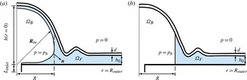
Radial cross-section of the elastic Hele-Shaw cell in (a) the Navier–Stokes model and (b) the lubrication model.

For the two-phase problem, we describe the position of the air–liquid interface
 $\partial {\it\Omega}_{BF}$
by a vector
 $\boldsymbol{R}_{in}(s,t)$
, parametrised by a surface coordinate
 $s$
, as shown in figure 3(a), and assume that the air–liquid interface remains pinned to the inlet so that
 $\boldsymbol{R}_{in}(s=0,t)=R_{inlet}\boldsymbol{e}_{r}$
. The kinematic boundary condition that links the fluid velocity to the motion of the air–liquid interface is then given by
 $$\begin{eqnarray}\boldsymbol{u}\boldsymbol{\cdot }\boldsymbol{n}=\frac{\partial \boldsymbol{R}_{in}}{\partial t}\boldsymbol{\cdot }\boldsymbol{n}\quad \text{on }\partial {\it\Omega}_{BF},\end{eqnarray}$$
where
 $\boldsymbol{n}$
is the unit vector normal to
 $\partial {\it\Omega}_{BF}$
(directed out of the fluid). This condition is augmented by the dynamic boundary condition
 $$\begin{eqnarray}\left(-p+{\it\mu}\left(\boldsymbol{{\rm\nabla}}\boldsymbol{u}+(\boldsymbol{{\rm\nabla}}\boldsymbol{u})^{\text{T}}\right)\right)\boldsymbol{n}+{\it\gamma}{\it\kappa}\boldsymbol{n}=-p_{b}\boldsymbol{n}\quad \text{on }\partial {\it\Omega}_{BF},\end{eqnarray}$$
where
 ${\it\kappa}$
is the sum of the principal curvatures of
 $\partial {\it\Omega}_{BF}$
and
 $p_{b}$
is the pressure in the expanding bubble. For simplicity, we truncate the fluid domain at
 $r=R_{outer}$
, where we impose purely radial outflow, and apply a radial traction that is consistent with a hydrostatic pressure distribution,
 $$\begin{eqnarray}u_{z}=0\quad \text{and}\quad -p+2{\it\mu}\frac{\partial u_{r}}{\partial r}={\it\rho}g(z-h)\quad \text{at }r=R_{outer},\end{eqnarray}$$
where
 $h(r,t)={\it\zeta}(r,t)+h_{0}$
is the depth of the cell and the reference pressure has been chosen such that for zero flow and zero fluid pressure, the membrane (which is subject to zero external pressure; see figure 3) is in equilibrium. Finally, we use the integral volume conservation equation for the bubble volume,
 $V_{B}(t)$
,
 $$\begin{eqnarray}\int _{{\it\Omega}_{B}}\text{d}V=V_{B}(t=0)+\dot{V}t,\end{eqnarray}$$
as the equation that determines the spatially uniform time-varying bubble pressure
 $p_{b}(t)$
.
3.1.2. Lubrication-theory model
Since the aspect ratio of the elastic-walled Hele-Shaw cells is small (
 $h_{0}/R_{outer}\ll 1$
), most previous studies (e.g. Michaut Reference Michaut2011; Al-Housseiny et al.
Reference Al-Housseiny, Christov and Stone2013; Lister et al.
Reference Lister, Peng and Neufeld2013; Pihler-Puzović et al.
Reference Pihler-Puzović, Périllat, Russell, Juel and Heil2013; Hewitt et al.
Reference Hewitt, Balmforth and de Bruyn2015) described the fluid flow by the Reynolds lubrication equation (Reynolds Reference Reynolds1886),
 $$\begin{eqnarray}\frac{\partial h}{\partial t}=\frac{1}{r}\frac{\partial }{\partial r}\left(\frac{rh^{3}}{12{\it\mu}}\frac{\partial }{\partial r}(\bar{p}+{\it\rho}gh)\right)\!,\end{eqnarray}$$
where
 $\bar{p}(r,t)$
is the component of the depth-averaged fluid pressure that excludes the contribution from the hydrostatic pressure.
We initially assume that in the two-phase problem the fluid films that are deposited on the upper and lower cell boundaries by the expanding bubble are sufficiently thin to be neglected, as shown in figure 3(b). This assumption will be re-examined in Part 2. The evolution of the thickness-averaged radius of the air–liquid interface,
 $R(t)$
, is then governed by the kinematic boundary condition
 $$\begin{eqnarray}\frac{\text{d}R}{\text{d}t}=\bar{u}_{r}|_{r=R(t)},\end{eqnarray}$$
where
 $$\begin{eqnarray}\bar{u}_{r}=-\frac{h^{2}}{12{\it\mu}}\frac{\partial }{\partial r}(\bar{p}+{\it\rho}gh)\end{eqnarray}$$
is the depth-averaged radial fluid velocity. To evaluate the dynamic boundary condition (3.8), we approximate the transverse component of the curvature as
 $2/h$
and neglect the viscous normal stresses to obtain
 $$\begin{eqnarray}p_{b}(t)-\bar{p}={\it\gamma}\left(\frac{1}{R}+\frac{2}{h}\right)\quad \text{at }r=R(t).\end{eqnarray}$$
We note that since
 $h\ll R$
, the first term on the right-hand side of this equation could have been neglected, but it was retained for consistency with our previous studies of non-axisymmetric fingering instabilities in which this azimuthal curvature term plays an important stabilising role. Within the framework of lubrication theory, the traction boundary condition at the outer boundary (3.9a,b
) corresponds to
 $$\begin{eqnarray}\bar{p}=0\quad \text{at }r=R_{outer},\end{eqnarray}$$
while the mass conservation equation (3.10) becomes
 $$\begin{eqnarray}2{\rm\pi}\int _{0}^{R_{outer}}h(r,t)\,r\,\text{d}r={\rm\pi}h_{0}R_{outer}^{2}+\dot{V}t.\end{eqnarray}$$
3.2. Membrane equations
In the experiments, the vertical deflection of the membrane
 ${\it\zeta}$
in response to the fluid pressure is much larger than its thickness
 $d$
. This suggests that self-induced in-plane stresses make an important contribution to the elastic response of the membrane. We therefore used the Föppl–von Kármán equations (Landau & Lifshitz Reference Landau and Lifshitz1970)
 $$\begin{eqnarray}\displaystyle & \displaystyle \frac{Ed^{3}}{12(1-{\it\nu}^{2})}\frac{1}{r}\frac{\partial }{\partial r}\left[r\frac{\partial }{\partial r}\left[\frac{1}{r}\frac{\partial }{\partial r}\left[r\frac{\partial {\it\zeta}}{\partial r}\right]\right]\right]-\frac{d}{r}\frac{\partial }{\partial r}\left[\frac{\partial {\it\zeta}}{\partial r}\frac{\partial {\it\phi}}{\partial r}\right]=P, & \displaystyle\end{eqnarray}$$
 $$\begin{eqnarray}\displaystyle & \displaystyle \frac{1}{r}\frac{\partial }{\partial r}\left[r\frac{\partial }{\partial r}\left[\frac{1}{r}\frac{\partial }{\partial r}\left[r\frac{\partial {\it\phi}}{\partial r}\right]\right]\right]+\frac{E}{r}\frac{\partial }{\partial r}\left[\frac{1}{2}\left(\frac{\partial {\it\zeta}}{\partial r}\right)^{2}\right]=0 & \displaystyle\end{eqnarray}$$
to describe the deformation of the membrane in response to the pressure
 $P$
exerted by the fluid. Here,
 ${\it\phi}$
is an Airy stress function for the non-zero components of the in-plane stress tensor such that
 ${\it\sigma}_{rr}=(1/r)(\partial {\it\phi}/\partial r)$
and
 ${\it\sigma}_{{\it\theta}{\it\theta}}=\partial ^{2}{\it\phi}/\partial r^{2}$
. In the experiments, the sheet was not subjected to any in-plane prestress, rested freely on the fluid layer and remained flat and undeformed at large distances from the injection point. This motivates the boundary conditions
 $$\begin{eqnarray}{\it\zeta}=\frac{\partial {\it\zeta}}{\partial r}={\it\phi}=\frac{\partial {\it\phi}}{\partial r}=0\quad \text{at }r=R_{outer}.\end{eqnarray}$$
The pressure
 $P$
in (3.17) is the pressure acting on the membrane – either the Navier–Stokes pressure, evaluated at the boundary,
 $p(r,z=h(r,t))$
, the lubrication pressure
 $\bar{p}$
or for the two-phase lubrication model
 $$\begin{eqnarray}P=\left\{\begin{array}{@{}ll@{}}p_{b} & \text{if }r<R(t),\\ \bar{p} & \text{if }r\geqslant R(t).\end{array}\right.\end{eqnarray}$$
3.3. Coupled solution
The governing equations for the Navier–Stokes- and lubrication-theory-based models were solved numerically using a fully coupled discretisation of the relevant fluid and solid equations. The Navier–Stokes-based model was implemented in oomph-lib (Heil & Hazel Reference Heil, Hazel, Schäfer and Bungartz2006) by discretising the weak form of the momentum and continuity equations (3.1)–(3.3) in their arbitrary Lagrangian–Eulerian (ALE) form on an unstructured moving mesh, using six-noded triangular Taylor–Hood finite elements (with continuous, piecewise linear and quadratic basis functions for the pressure and velocity components respectively). The mesh was generated using Shewchuk’s (Reference Shewchuk, Lin and Manocha1996) unstructured mesh generator, Triangle. The implicit, second-order accurate, adaptive BDF2 scheme was employed to discretise all time derivatives. The dynamic boundary condition (3.8) for the two-phase flow problem was incorporated via the boundary integral that appears naturally in the weak form of the Navier–Stokes equations. The mesh deformation in response to the motion of the bounding membrane (and, in the two-phase flow problem, the displacement of the air–liquid interface) was determined by treating the fluid mesh as an elastic solid whose deformation is determined by the equations of large-displacement elasticity. Lagrange multipliers were used to enforce the boundary displacements such that the normal motion of the air–liquid interface satisfied the kinematic boundary condition (3.7) and that nodes that were located on the elastic membrane were displaced vertically to remain in contact with the membrane. The fluid domain was remeshed after every few time steps to avoid the excessive distortion of elements. The size of the elements in the new mesh was determined by the Z2 error estimator (Zienkiewicz & Zhu Reference Zienkiewicz and Zhu1992), and the solution was transferred to the new mesh by projection. In the interest of brevity, we omit details but refer to Hazel et al. (Reference Hazel, Heil, Waters and Oliver2012), where an equivalent discretisation of the axisymmetric free-surface Navier–Stokes equations was used in a different problem. While Triangle is able to generate high-quality meshes throughout the fluid domain, a technical difficulty arises in the two-phase flow problem in the region near the inlet where the free surface is pinned at
 $(r,z)=(R_{inlet},0)$
. At large times, the liquid film deposited on the lower wall becomes very thin and almost parallel to the wall (see figure 5). As a result, the fluid domain terminates in a very shallow angle. Since such regions can only be meshed with strongly distorted elements, we surrounded the inlet by a shallow groove in the bottom plate (which is just about visible in the inset in figure 5), whose presence had no effect on the solution but allowed us to maintain the mesh quality throughout the fluid domain. The Föppl–von Kármán equations were discretised by a mixed finite-element method in which we approximated the vertical displacements
 ${\it\zeta}$
, the Airy stress functions
 ${\it\phi}$
and their respective Laplacians by piecewise quadratic basis functions, defined on three-noded one-dimensional elements. Again, we omit details but refer to Pihler-Puzović et al. (Reference Pihler-Puzović, Périllat, Russell, Juel and Heil2013) for a more detailed discussion of the implementation. The fully coupled implicit discretisation of the fluid and solid equations produces a large system of nonlinear algebraic equations at each time step. This system was solved by Newton’s method, using SuperLU (Demmel et al.
Reference Demmel, Eisenstat, Gilbert, Li and Liu1999) as the linear solver.
The lubrication-theory model was discretised by a second-order accurate finite-difference scheme and implemented in MatLab; see Pihler-Puzović et al. (Reference Pihler-Puzović, Périllat, Russell, Juel and Heil2013) for details. The inflation of the membrane under constant pressure, discussed in § 4.1 below, was also simulated using the same finite-difference discretisation in MatLab.
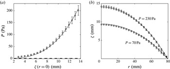
(a) Vertical displacement of the latex sheet at the centre of the cell
 ${\it\zeta}(r=0)$
as a function of the spatially uniform pressure
 $P$
, obtained experimentally (circles), by solving the Föppl–von Kármán equations (solid line) and by solving the linear bending equations (dashed line). (b) The spatial variation of the vertical displacement of the sheet across the latex cell for two different pressures
 $P=70$
Pa and
 $P=230$
Pa, obtained experimentally (circles) and by solving the Föppl–von Kármán equations (solid lines).

4. Results
4.1. Membrane inflation
Before analysing the fully coupled fluid–structure interaction problem, we wish to assess how well the Föppl–von Kármán equations describe the elastic deformation of the membrane. For this purpose we changed the experimental set-up slightly and clamped the elastic sheet to the bottom plate using a thick-walled metal ring of radius
 $R_{cell}=8$
cm. The sheet was then inflated slowly by injecting air. We monitored the difference
 $P$
between the pressure inside the cell and the atmospheric pressure with an ultralow-pressure sensor (pressure range
 $\pm 625$
Pa, Honeywell), calibrated with a U-tube manometer filled with water over its entire range of operation. Figure 4(a) illustrates the load–displacement characteristics for the latex sheet by plotting the pressure
 $P$
as a function of the sheet’s vertical displacement at the centre
 ${\it\zeta}(r=0)$
, while figure 4(b) shows the spatial variation of the sheet’s vertical displacement across the cell for two different pressures. The symbols represent experimental measurements, with error bars indicating the standard error of the mean value over five experiments. The solid lines show the results obtained from the numerical solution of the Föppl–von Kármán equations for a Young’s modulus of
 $E=2.1$
MPa. They are in excellent agreement with the experimental measurements over the whole range of displacements encountered in the fluid–structure interaction experiments presented below. In the case of the polypropylene sheet, we obtained a similar level of agreement for a Young’s modulus of
 $E=3.7$
GPa. This gives us confidence that the Föppl–von Kármán equations provide a good description of the membrane’s elastic behaviour in the experiments reported in this paper. We note, however, that the two Young’s moduli (which are the only fitted parameters in our model) are larger by a factor of approximately 1.5 than the values measured by us using extensometry (Pihler-Puzović et al.
Reference Pihler-Puzović, Illien, Heil and Juel2012). We will return to this issue in §§ 4.2.1 and 5.
To assess the importance of the self-induced in-plane stresses relative to the bending stiffness of the sheet, the thick dashed line in figure 4(a) shows a plot of the load–displacement curve corresponding to a linear bending model (obtained by setting
 ${\it\phi}=0$
in (3.17) and (3.18)). The comparison between the two curves demonstrates that the elastic response of the membrane is dominated by the self-induced in-plane stresses once the deflection of the sheet in the centre exceeds a value of
 ${\approx}1.5$
mm, as expected when
 $h\gg d$
. We note that in the fluid–structure interaction experiments shown in the next section (and also in the experiments reported in our earlier paper, Pihler-Puzović et al. (Reference Pihler-Puzović, Illien, Heil and Juel2012)) the membrane was subjected to much larger deformations, suggesting that self-induced tensions must be represented in any theoretical model. These measurements thus support the membrane-modelling assumptions of Lister et al. (Reference Lister, Peng and Neufeld2013) over those of Al-Housseiny et al. (Reference Al-Housseiny, Christov and Stone2013).
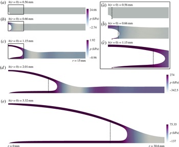
Instantaneous cross-sectional profiles of the elastic-walled Hele-Shaw cell and the corresponding pressure fields during the two-phase displacement flow under the latex sheet for
 $\dot{V}=150~\text{ml}~\text{min}^{-1}$
at
 $t$
equal to (a) 0 s, (b) 0.0001 s, (c) 0.005 s, (d) 0.1 s and (e) 1 s, computed in simulations of the Navier–Stokes model. The inset enumerated as (
 $\tilde{a}$
)–(
 $\tilde{c}$
) shows the details of the profiles from (a) to (c) in the bubble region. The instantaneous positions of the interface computed using the lubrication model are indicated with the dashed lines.

4.2. Fluid–structure interaction
Next, we consider the fully coupled fluid–structure interaction problem in which the gap under the membrane is initially filled with viscous fluid.
Instantaneous cross-sectional profiles of the elastic-walled Hele-Shaw cell during the two-phase displacement flow under the latex sheet for
 $\dot{V}=150~\text{ml}~\text{min}^{-1}$
at
 $t=4$
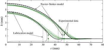
s (lower curves) and 10 s (upper curves), found experimentally (discrete data with error bars), and computed using the Navier–Stokes model (solid lines) and the lubrication model (dashed lines). The experimental points were obtained by averaging the data from six different experimental runs, with the error bars indicating the standard error of the measured mean values.

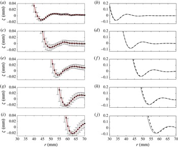
The scaled instantaneous profiles from the experiments (a,c,e,g,i) and the numerical simulations using the Navier–Stokes (solid lines, b,d,f,h,j) and lubrication (dashed lines, b,d,f,h,j) models. The profiles correspond to the elastic-walled Hele-Shaw cell with the latex sheet from figure 6 at 2 s (a,b), 4 s (c,d), 6 s (e,f), 8 s (g,h) and 10 s (i,j) from the start of the air injection. As in figure 6, the experimental points were obtained by averaging the data from six different experimental runs, with the error bars indicating the standard error of the measured mean values. The lines connecting the experimental data points are drawn to guide the eye. We note the different vertical axis ranges in (a,c,e,g,i) and (b,d,f,h,j).

4.2.1. The two-phase flow
Figure 5 illustrates the evolution of the fluid domain following the start of the gas injection at a constant rate of
 $\dot{V}=150~\text{ml}~\text{min}^{-1}$
, using results from the Navier–Stokes simulations.
Initially, the bubble expands uniformly in all directions and causes only a modest localised inflation of the membrane near the centre of the cell. Once the size of the bubble becomes comparable to the cell depth, the bubble begins to expand predominantly in the radial direction while depositing a static film of viscous fluid on the upper and lower cell boundaries. The membrane continues to inflate slowly while the bubble expands, ‘peeling’ apart the cell boundaries in a manner that is reminiscent of the behaviour observed in 2D (and 3D) studies of pulmonary airway reopening (Perun & Gaver III Reference Perun and Gaver III1985, Reference Perun and Gaver III1995; Gaver III et al. Reference Gaver III, Samsel and Solway1990, Reference Gaver III, Halpern, Jensen and Grotberg1996; Heil Reference Heil, King and Shikmurzaev2001; Jensen et al. Reference Jensen, Horsburgh, Halpern and Gaver2002; Hazel & Heil Reference Hazel and Heil2003, Reference Hazel and Heil2008; Grotberg & Jensen Reference Grotberg and Jensen2004; Juel & Heap Reference Juel and Heap2007; Heap & Juel Reference Heap and Juel2008; Heil & Hazel Reference Heil and Hazel2011). We note, in particular, the minimum in the fluid pressure ahead of the bubble tip which creates a local minimum in the cell depth (sometimes referred to as a ‘neck’ in the airway reopening literature) in a manner similar to the behaviour observed in the peeling of an inextensible flexible tape (McEwan & Taylor Reference McEwan and Taylor1966) and in peeling of a thick sheet by bending stresses (Lister et al. Reference Lister, Peng and Neufeld2013). Careful inspection of the displacement field shows that this ‘neck’ is in fact the first minimum of a decaying oscillatory displacement pattern ahead of the bubble tip which we will analyse in more detail below. The vertical lines in figure 5 indicate the bubble radius predicted by the lubrication-theory model discussed in § 3.1.2. Since this model ignores the presence of the fluid films that are deposited on the upper and lower cell boundaries, it significantly underestimates the bubble radius. We will return to this issue in Part 2.
Figure 6 shows a direct comparison between the computational predictions and the experimental measurements by plotting the shape of the membrane and the position of the air–liquid interface 4 and 10 s after the start of the injection. The vertical lines in figure 6 indicate the positions of the bubble radius
 $R(t)$
found in the experiments and predicted by the lubrication model. The agreement between the different sets of results is very good, with the computational predictions for the membrane position obtained from the Navier–Stokes computations generally being close to (or even within) the experimental error bars. The most significant discrepancy arises in the region just ahead of the bubble tip where the membrane is bent less strongly in the experiments. Possibly as a result, the amplitude of the wave pattern ahead of the bubble tip is much smaller (and, in fact, barely visible) in the experimental data in figure 6. In figure 7, we therefore show an enlargement of the wall displacement field in the vicinity of the bubble tip to demonstrate that the wave pattern is, in fact, present in all data sets. Its key characteristics, namely the wavelength (judged by a half-wavelength of approximately 7 mm between successive peaks) and its decay rate (estimated from the reduction in the amplitude of the successive peaks to be
 ${\approx}0.13~\text{mm}^{-1}$
), are in excellent agreement. Given that both theoretical models are based on the same wall equations and that they agree very well with each other, we conjecture that the discrepancy between theory and experiments might be due to the use of the Föppl–von Kármán equations, rather than the full equations of elasticity; see § 5 for a more detailed discussion of this issue.
The instantaneous pressure
 $P$
at
 $t=10$
s in the two-phase flow for
 $\dot{V}=150~\text{ml}~\text{min}^{-1}$
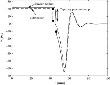
under the latex membrane, computed using the Navier–Stokes and lubrication models. The filled circle and squares show the position of the bubble tip in the Navier–Stokes and lubrication-theory models respectively.

A curious feature of figures 6 and 7 is that the membrane shapes predicted by the lubrication and Navier–Stokes models agree extremely well, despite the fact that the predictions of the models for the radius of the air–liquid interface differ significantly; see figure 6 (and also figure 9 below). To investigate the reason for this agreement, figure 8 compares the instantaneous fluid pressure distribution acting on the membrane at
 $t=10$
s predicted by the two models. In both models, the fluid is subject to the same boundary condition at
 $r=R_{outer}$
where the fluid pressure is set to zero. Lubrication theory can be expected to provide a good description of the pressure distribution in the region ahead of the bubble tip where the cell depth and its radial derivative are small; the agreement between the two models is indeed very good in this region. A noticeable discrepancy arises in the vicinity of the bubble tip. There, the Navier–Stokes model predicts a continuous increase in the fluid pressure, which arises through a combination of capillary effects and the viscous stresses at the air–liquid interface, as well as in the pressure gradient in the bulk required to redirect the fluid into the thin static liquid films that are deposited on the cell boundaries. Within these films the fluid pressure rapidly approaches a constant value, close to the bubble pressure. Conversely, in the lubrication model, the pressure gradient decreases as we approach the air–liquid interface because the increase in cell depth reduces the flow resistance; see (3.13). At
 $r=R$
, the capillary pressure jump (from (3.14)) then changes the fluid pressure discontinuously to the spatially constant bubble pressure in the region
 $r<R$
. Figure 8 shows that the good overall agreement between the two models is at least partly due to a fortuitous cancellation of errors – the capillary pressure jump alone, applied at the wrong (smaller) radius, results in approximately the same final bubble pressure as that predicted by the full Navier–Stokes model. Figure 7 shows that the predicted locations of the peeling wave in the lubrication and Navier–Stokes models are almost exactly the same even though the bubble radii are different, which supports the argument of Lister et al. (Reference Lister, Peng and Neufeld2013) that the spreading is largely controlled by the dynamics of peeling independent of the air–liquid interface.
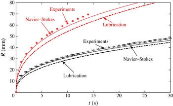
Figure 9 shows the evolution of the bubble radius for the largest and smallest injection flow rates imposed in the experiments,
 $\dot{V}=50~\text{ml}~\text{min}^{-1}$
and
 $\dot{V}=300~\text{ml}~\text{min}^{-1}$
respectively. The agreement between the Navier–Stokes simulations and the experimental measurements is excellent throughout, with a maximum discrepancy of 3 % over the whole range of experimental measurements, which were terminated when the bubble reached a radius of
 $R_{max}=70$
mm. As already noticed above, lubrication theory systematically underestimates the bubble radius, with the discrepancy to the experimental measurements increasing with an increase in the injection flow rate. This is because at larger flow rates (larger capillary numbers) the thickness of the films deposited on the cell walls increases, making the error in the mass conservation equation (3.16), which ignores the presence of these films, increasingly significant.
The time evolution of the interface in the two-phase displacement flow in the elastic-walled Hele-Shaw cell with the latex sheet for
 $\dot{V}=50~\text{ml}~\text{min}^{-1}$
(lower set of data) and
 $\dot{V}=300~\text{ml}~\text{min}^{-1}$
(upper set of data). The discrete points were obtained experimentally (the means and error bars were determined as described in the caption to figure 6 and § 2), while the lines correspond to predictions of different models, as indicated in the plot.

4.2.2. Scaling laws and the relation between single- and two-phase flows
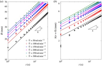
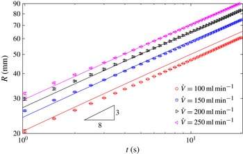
Figure 10(a) shows a log–log plot of the interfacial position (using data from the experiments with latex membranes and the corresponding Navier–Stokes simulations) for a much wider range of injection flow rates. Figure 11 shows the same comparison for the experiments with the much thinner but more rigid polypropylene sheets, whose stretching-to-bending ratio
 $12(1-{\it\nu}^{2})(h/d)^{2}$
is approximately 100 times larger than that of the latex sheets. This implies that at comparable deformations the self-induced tension in the polypropylene sheets is expected to make an even more significant contribution to the elastic forces in the membrane than in the experiments with the latex sheets.
The time evolution on a log–log scale of (a) the interface radius and (b) the cell depth at
 $r=0$
in the two-phase displacement flow in the elastic-walled Hele-Shaw cell with the latex sheet for a range of injection rates, obtained experimentally (discrete points obtained by averaging the data from six different experimental runs, with error bars indicating the standard error) and using the Navier–Stokes model (solid lines).

The time evolution on a log–log scale of the interface radius in the elastic-walled Hele-Shaw cell with the polypropylene sheet for a range of injection rates, obtained experimentally (discrete points found as in figure 10) and using the Navier–Stokes model (solid lines).

Figures 10(a) and 11 show that in both sets of experiments which were performed with fluids and membranes of vastly different properties, log–log plots of the bubble radius as a function of time are approximately straight lines, suggesting a power-law behaviour of the form
 $R(t)\sim t^{{\it\alpha}}$
. A curve fit to the experimental data shows that the power-law exponent
 ${\it\alpha}$
varies slightly between the two sets of experiments (
 ${\it\alpha}=0.368\pm 0.005$
and
 $0.387\pm 0.004$
for the latex and polypropylene sheets respectively, where the error corresponds to the standard deviation over six and four least-square power-law fits to the experimental data in figures 10(a) and 11 respectively; the difference between these two values is significant when compared with the experimental and fitting errors). Motivated by this observation we re-examined the computational data in figure 3(c) of Pihler-Puzović et al. (Reference Pihler-Puzović, Périllat, Russell, Juel and Heil2013), which shows the evolution of the bubble radius as a function of time for various values of the elastic modulus. When replotted on log–log axes these data also display a power-law behaviour, with the power-law exponent again depending on the properties of the elastic membrane. Specifically, an increase in Young’s modulus (while keeping all other parameters constant) is found to cause an increase in
 ${\it\alpha}$
. (We note that if the Young’s modulus is increased to such an extent that the membrane becomes effectively rigid,
 ${\it\alpha}$
will approach
 $1/2$
, since for a constant injection flow rate the bubble radius must vary like
 $R(t)\sim t^{1/2}$
to conserve mass.) The variations in
 ${\it\alpha}$
in figures 10(a) and 11 are small, however, and show that the behaviour is close to
 $R(t)\sim t^{3/8}$
for both sets of experiments. The evolution of the cell depth (which was only measured in the experiments with the latex sheet; see § 2) closely follows a power law of the form
 $h(r=0,t)\sim t^{1/4}$
; see figure 10(b).
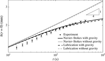
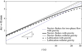
These power laws agree with those predicted by Lister et al.’s (Reference Lister, Peng and Neufeld2013) asymptotic analyses of the tension-dominated ‘peeling-by-pulling’ problem. Lister et al. (Reference Lister, Peng and Neufeld2013) argued that the same spreading laws should arise in both the single- and two-phase problems on the grounds that the rate of spread is controlled by the viscous fluid in the peeling region, so that the details of the flow in the central region are irrelevant. Given the excellent agreement between experiment, computations and asymptotic predictions in the two-phase problem, one might therefore expect Lister et al.’s (Reference Lister, Peng and Neufeld2013) predictions to do equally well (or better) when applied to the simpler single-phase problem. However, somewhat surprisingly, figure 12 indicates that this is not the case. The figure shows experimental measurements of the depth of the viscous fluid layer at the centre of the cell,
 $h(r=0,t)$
, for the case when silicone oil is injected at a constant flow rate of
 $\dot{V}=1~\text{ml}~\text{min}^{-1}$
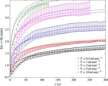
into a cell that is bounded by a latex sheet. The experimental measurements are in excellent agreement with the computational predictions based on the full Navier–Stokes model and lubrication theory, but neither data set follows the power-law behaviour observed for the two-phase flow. Furthermore, the agreement between the experiments and the theoretical calculations remains excellent over the whole range of injection rates accessible experimentally (figure 13).
The time evolution of the cell depth at
 $r=0$
on a log–log scale in the single-phase displacement flow for
 $\dot{V}=1~\text{ml}~\text{min}^{-1}$
under the latex sheet, obtained experimentally (see § 2 and the caption to figure 6 for details) and using the Navier–Stokes- and lubrication-theory-based models with and without the contribution from gravity.

The time evolution of the cell depth at
 $r=0$
in the single-phase displacement flow in the elastic-walled Hele-Shaw cell with the latex sheet for a range of injection rates, obtained experimentally (discrete points found by averaging the data from six different experimental runs, with error bars indicating the standard error) and from the Navier–Stokes- (solid lines) and lubrication-theory-based (dashed lines) models.

The main reason for this discrepancy is evident from the second set of computational results shown in figure 12. The thinner lines show the results obtained from the Navier–Stokes and lubrication models if gravity (which is not included in Lister et al.’s (Reference Lister, Peng and Neufeld2013) analysis of tension-driven spreading) is neglected by setting
 $g=0$
in (3.2), (3.9a,b
), (3.11) and (3.13). In this case, we recover the power-law behaviour,
 $h(r=0,t)\sim t^{1/4}$
, predicted by the theory. This suggests that gravitational slumping of the central bulge, driven by the radial gradient of the hydrostatic pressure, plays a much more important role in the single-phase system than in its two-phase counterpart. This is because in the single-phase problem the hydrostatic pressure results from the entire depth of the continuous viscous fluid layer, rather than from the two relatively thin viscous films that are deposited on the upper and lower cell boundaries in the two-phase problem. The resulting gravity-driven slumping flow augments the radial spreading driven by the elastic pressure and therefore reduces the depth of the viscous layer relative to that of a flow without gravity. The deviation from the behaviour for zero gravity increases with time because the tension in the sheet decreases near the injection point and the hydrostatic pressure gradients become dominant. We refer to Lister et al. (Reference Lister, Peng and Neufeld2013) for an asymptotic analysis of this gravitational effect for the case when the stiffness of the sheet is dominated by bending, and to Hewitt et al. (Reference Hewitt, Balmforth and de Bruyn2015) for the case of tension-dominated spreading in two dimensions.
While gravity is the main reason for the non-power-law behaviour of
 $h(0,t)$
, it is not the only significant difference between the single- and two-phase problems. The injection rates used in our single-phase experiments (figure 13) are necessarily much smaller than those used in the two-phase experiments (figures 10 and 11) because the injection of viscous fluid into the elastic-walled Hele-Shaw cell requires much larger pressures which rapidly exceed those that can be generated by our volumetric pump; see the discussion in § 2. However, we can compare the problems computationally at the same injection rate.
The time evolution of the cell depth at
 $r=0$
on a log–log scale in the single-phase and two-phase displacement flows for
 $\dot{V}=50~\text{ml}~\text{min}^{-1}$
under the latex sheet, using the Navier–Stokes- and lubrication-theory-based models, with and without the contribution from gravity. If not stated otherwise, the results for the single-phase flow are shown.

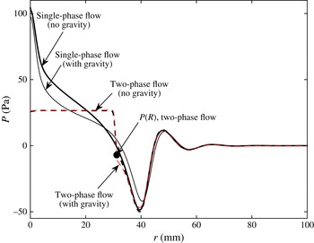
The instantaneous pressure
 $P$
at
 $t=10$
s in the single-phase (solid lines) and two-phase (dashed lines) flows at
 $\dot{V}=50~\text{ml}~\text{min}^{-1}$
under the latex membrane, computed using the Navier–Stokes-based model, with and without gravity.

Figure 14 shows that gravity has the same qualitative effect on the behaviour of
 $h(0,t)$
in single-phase flow at the flow rate of
 $\dot{V}=50~\text{ml}~\text{min}^{-1}$
as it did in single-phase flow at the lower experimental flow rate of
 $\dot{V}=1~\text{ml}~\text{min}^{-1}$
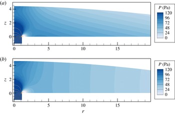
(cf. figure 12). It also shows that the central cell height is distinctly larger for single-phase flow than for two-phase flow, except at late times when the gravitational spreading becomes dominant. Figure 15 provides a detailed comparison between the computed fluid pressure distributions that act on the membrane for the cases of single- and two-phase flows (solid and dashed lines) and when gravity is included (thin lines) or neglected (thick lines). As expected, gravity has a stronger effect on the pressure distribution (and therefore the membrane deformation) in the single-phase than in the two-phase system. However, the most striking feature of figure 15 is not the effect of gravity but the difference between the pressure distributions for the single- and two-phase flows in the central part of the cell. As discussed above in § 4.2.1, in the two-phase flow this region is occupied by an inviscid gas bubble whose spatially constant pressure is transmitted to the membrane through the static fluid layer that lines the membrane. In the single-phase case, there is a significant rise in fluid pressure towards the injection point, because the injection of viscous fluid into the relatively narrow gap between the upper and lower cell boundaries induces a large radial pressure gradient. A further rise in pressure occurs near the injection point where the fluid has to be deflected from its vertically upward motion into the radial direction. The viscous and gravitational pressure gradients can clearly be seen in the pressure contour plots in figure 16.
Contours of fluid pressure at
 $t=10$
s obtained in the Navier–Stokes simulations of the single-phase flow under the latex membrane at
 $\dot{V}=50~\text{ml}~\text{min}^{-1}$
(a) when gravity is accounted for and (b) when gravity is neglected. The colour contours show the fluid pressure using equally spaced increments over a limited range between 0 and 120 Pa. The pressure variations are much greater near the inlet, where we indicate the pressure distribution by pressure isolines that are equally spaced between
 $-1200$
and 2000 Pa in increments of 200 Pa.

It is quite remarkable that, despite the significant differences in the radial pressure distribution in the central part of the flow, the radial position of the frontal peeling wave is almost exactly the same in the single- and two-phase cases. Figure 14 clearly shows that the large central pressures in single-phase flow have a significant effect on the central height of the membrane. In the two-phase system, viscous pressure gradients in the central part of the cell and vertical pressure gradients induced by gravity are almost absent. By contrast, an accurate description of the single-phase flows in elastic-walled Hele-Shaw cells requires these effects to be included – at least in the parameter regime considered here.
5. Discussion and conclusions
We have performed a detailed experimental and numerical study of single- and two-phase displacement flows in elastic-walled Hele-Shaw cells in order to identify the dominant mechanisms that control the behaviour of the system. We established that in the parameter regime considered here (and in previous studies, such as Pihler-Puzović et al. (Reference Pihler-Puzović, Illien, Heil and Juel2012)), the stiffness of the elastic membrane that forms the upper boundary of the cell has significant contributions both from its self-induced in-plane tension and from bending effects. Overall, the Föppl–von Kármán equations were found to provide a good description of the membrane’s deformation in this regime. The main discrepancy between the experimentally observed and computed wall shapes arises in the amplitude of the wave pattern in the region ahead of the bubble tip. We suspect that this might be due to geometric or constitutive nonlinearities that are not captured by the Föppl–von Kármán theory. In fact, we have already pointed out that the Young’s moduli that we obtained by fitting the Föppl–von Kármán model to the experimental results for the sheet inflation are somewhat larger than those typically reported in the literature. This suggests that the Young’s moduli required to obtain the excellent agreement between theory and experiment in the sheet inflation experiments (as shown in figure 4) may compensate for constitutive nonlinearities of the actual material. It is, however, interesting to note that changes in Young’s modulus have very little effect on the wall deformation in the fluid–structure interaction simulations. For instance, decreasing the Young’s modulus by a factor of 1.5 results in less than 2 % change in the evolution of the interface radii for the cases shown in figure 9.
We performed a critical assessment of lubrication-theory-based models that were used in most previous theoretical studies of this problem. We showed that in the case of two-phase flow, when the injected fluid is an inviscid gas, the lubrication-theory-based predictions for the evolution of the bubble radius
 $R(t)$
are in reasonable qualitative agreement with the Navier–Stokes-based results. The discrepancy between the two models can be attributed primarily to the neglect in the lubrication model of the thin layers of viscous fluid that are deposited on the upper and lower boundaries of the Hele-Shaw cell and, to a lesser extent, to the rather simplistic model for the visco-capillary flow in the vicinity of the gas–liquid interface. This is consistent with the results of previous studies that used a matched asymptotics approach in which numerical computations near the bubble rim were coupled to lubrication theory away from the interface (Jensen et al.
Reference Jensen, Horsburgh, Halpern and Gaver2002). The difference in the instantaneous bubble radius
 $R(t)$
predicted by our two models increases continuously and can become as large as 16 % for the parameter range considered here. However, log–log plots of the
 $R(t)$
data from the experiments and the Navier–Stokes computations, obtained for widely different membrane properties, are nevertheless close to the power-law behaviour predicted by Lister et al.’s (Reference Lister, Peng and Neufeld2013) lubrication-theory-based asymptotic model.
In the case of single-phase flow, the absence of the gas–liquid interface implies that the lubrication-theory-based model predictions by Lister et al. (Reference Lister, Peng and Neufeld2013) might naively be expected to agree better with experiments. However, we found that for the range of parameters considered here the gravitational pressure variation in the region where the membrane is strongly inflated plays an important role and that the viscous pressure gradient remains sufficiently large throughout the domain that it cannot be neglected anywhere. While both of these effects are easily included into the lubrication-theory model (see, e.g., Hewitt et al. Reference Hewitt, Balmforth and de Bruyn2015), they are shown here to have a strong effect on the system’s behaviour, causing it to deviate significantly from the power-law behaviour predicted by Lister et al.’s (Reference Lister, Peng and Neufeld2013) asymptotic solution.
In Part 2 of this paper we use the insight gained from the experimental and computational studies presented here to develop an improved lubrication-theory-based model that uses results from Reinelt & Saffman (Reference Reinelt and Saffman1985) to derive corrections to the kinematic and dynamic boundary conditions (3.12) and (3.14) at the air–liquid interface. We show that this model yields results that are in excellent agreement with those of the Navier–Stokes-based model. The lubrication-theory model is then used to develop asymptotic descriptions of the system’s behaviour in specific regions of parameter space. We anticipate that it may also form a promising starting point for a theoretical analysis of the non-axisymmetric fingering and wrinkling instabilities reported in Pihler-Puzović et al. (Reference Pihler-Puzović, Illien, Heil and Juel2012, Reference Pihler-Puzović, Périllat, Russell, Juel and Heil2013) and Pihler-Puzović, Juel & Heil (Reference Pihler-Puzović, Juel and Heil2014).
Acknowledgements
The authors thank A. Hazel for many helpful discussions and acknowledge early contributions of R. Anankine, D. Edmunds and S. McMorris to some of the experimental results presented here. The work of D.P.P., A.J. and M.H. was funded through EPSRC grant EP/J007927/1 and G.G.P. was supported by an EPSRC PhD studentship. The research data supporting this publication are available in the supplementary material at http://dx.doi.org/10.1017/jfm.2015.590.
Supplementary data
Supplementary data is available at http://dx.doi.org/10.1017/jfm.2015.590.