





1 Introduction
In educational testing, item response theory (IRT) models are commonly used to estimate a test-taker’s latent ability. With the widespread use of computerized testing, there has been a growing interest in using response time data as collateral information to improve the accuracy of ability estimates in IRT modeling (van der Linden et al., Reference van der Linden, Klein Entink and Fox2010). The most commonly adopted approach is the hierarchical modeling approach (van der Linden, Reference van der Linden2007). At the first level, the conditional distributions of observed item responses and response times given the latent ability and speed are defined. At the second level, the latent traits are assumed to follow a multivariate normal (MVN) distribution, a convenient but often unrealistic assumption.
Poor model fit of the hierarchical model to empirical data has been discussed in the literature, suggesting that the dependence between responses and response times is not fully captured by the model (e.g., Bolsinova et al., Reference Bolsinova, De Boeck and Tijmstra2017; Domingue et al., Reference Domingue, Kanopka, Stenhaug, Sulik, Beverly, Brinkhuis, Circi, Faul, Liao, McCandliss, Obradovic, Piech, Porter, Soland, Weeks, Wise and Yeatman2022; Liu & Wang, Reference Liu and Wang2024). Alternative modeling approaches have been proposed to address these limitations (e.g., Bolsinova et al., Reference Bolsinova, De Boeck and Tijmstra2017; Braeken et al., Reference Braeken, Tuerlinckx and De Boeck2007; Kang et al., Reference Kang, Jeon and Partchev2023; Liu & Wang, Reference Liu and Wang2024). One line of research relaxes the conditional independence assumption between item responses and response times given the latent traits. For example, Bolsinova et al. (Reference Bolsinova, De Boeck and Tijmstra2017) explicitly model the conditional dependence (CD) between item response and response time by incorporating the residual log-response time as a covariate of the IRT model parameters. Kang et al. (Reference Kang, De Boeck and Ratcliff2022, Reference Kang, Jeon and Partchev2023) introduce diffusion IRT (DIRT) models that allow for CD between responses and response times by incorporating within-person variation in cognitive components into traditional IRT models. Another line of research tackles the parametric assumptions of the hierarchical model. For instance, Liu and Wang (Reference Liu and Wang2024) propose a semi-parametric factor analysis framework that more flexibly models the joint distribution of responses and response times.
This study addresses the potential violation of the structural multivariate normality assumption for latent traits, particularly when dependence is stronger at one extreme of the distribution. Modeling asymmetry has generated recent interest in the IRT literature, specifically regarding asymmetric item characteristic curves (Bolt & Liao, Reference Bolt and Liao2022; Lee & Bolt, Reference Lee and Bolt2018). However, this study focuses on the structural asymmetric dependence between latent traits. Asymmetric dependence between speed and accuracy can manifest at two distinct levels: within-person and population. At the within-person level, for instance, Domingue et al. (Reference Domingue, Kanopka, Stenhaug, Sulik, Beverly, Brinkhuis, Circi, Faul, Liao, McCandliss, Obradovic, Piech, Porter, Soland, Weeks, Wise and Yeatman2022) analyzed 29 empirical cognitive test datasets and found a consistent pattern in the speed–accuracy trade-off. There is a larger variance in the lower tail, that is, individuals who receive lower estimates of ability tend to vary their speed more. On the other hand, at the population level (van der Linden, Reference van der Linden2007), asymmetric dependence occurs when the strength of dependence between ability and speed varies across the latent spectrum, in particular, the dependence between speed and ability can be stronger at one extreme of the distribution than the other. The current study focuses on the population level, assuming that while an individual’s latent speed is fixed across items, there is an asymmetric dependence between latent speed and ability across the population.
We present a copula-based joint model for speed and accuracy within the IRT framework. Rather than modeling conditional dependency between responses and response times, our approach addresses this model misfit by introducing a more flexible dependence structure between the latent traits themselves. The proposed model uses a copula function to specify the joint distribution of latent ability and speed, allowing for asymmetric, stronger tail-dependence structures as exemplified in Figure 1. This flexibility is expected to yield improved model fit with empirical data compared to the model based on the MVN distribution while preserving the original measurement models for the conditional distributions of item response and response times (e.g., two-parameter logistic model [2PL] and log-normal model).
Bivariate distributions constructed with copula functions and standard normal margins.
Note: X and Y were simulated using a bivariate copula with standard normal marginal distributions. The red contours represent the bivariate density, and the dots indicate the randomly simulated data points.

Figure 1 Long description
The figure consists of six panels arranged in two rows and three columns. Each panel has an x-axis and y-axis ranging from minus 2 to 2 with a grid background. Red concentric contour lines represent density, and grey dots represent simulated data points.
Top-left panel, Independence. The red contours are perfectly circular and centered at 0, 0. Data points are evenly scattered in a circular cloud.
Top-center panel, Gaussian. The red contours form an ellipse tilted at a 45-degree angle, indicating a linear correlation. Data points follow this diagonal elliptical shape.
Top-right panel, Frank. Similar to Gaussian, the contours are elliptical and tilted at 45 degrees, but the density is slightly more concentrated in the center.
Bottom-left panel, Clayton. The red contours are asymmetrical, narrowing to a sharp point in the bottom-left quadrant (negative tail) and broadening in the top-right. This indicates strong lower-tail dependence.
Bottom-center panel, Gumbel. The red contours are asymmetrical, narrowing to a sharp point in the top-right quadrant (positive tail) and broadening in the bottom-left. This indicates strong upper-tail dependence.
Bottom-right panel, Joe. Similar to Gumbel, the contours show even sharper narrowing toward the top-right quadrant, indicating very strong upper-tail dependence.
Copula-based dependence models, particularly asymmetric and heavy-tailed copulas, have become powerful tools in econometrics, finance, and survival analysis, addressing limitations of traditional multivariate modeling approaches (see reviews by Genest et al., Reference Genest, Okhrin and Bodnar2024 and Ghosh et al., Reference Ghosh, Sheppard, Holder, Loecke, Reid, Bever and Reuman2020). In finance, for instance, copulas have been used to model default dependence between financial institutions (Zhang et al., Reference Zhang, Kim, Yan and Zhao2024) and among bundled insurance risks (Shi & Zhao, Reference Shi and Zhao2024). Similarly, in survival analysis, they have been applied to model the dependence between tumor progression and patient mortality (Emura et al., Reference Emura, Nakatochi, Murotani and Rondeau2017). A seminal turning point was the 2008 global financial crisis, which exposed critical flaws in relying on Gaussian copulas to model dependencies such as those among corporate defaults (Donnelly & Embrechts, Reference Donnelly and Embrechts2010). During financial crises, corporate defaults occur in clusters, meaning the default of one company significantly increases the likelihood of defaults among interconnected companies. However, a key limitation of the Gaussian copula is its assumption of asymptotic independence in the extreme ends (Donnelly & Embrechts, Reference Donnelly and Embrechts2010), meaning it is mathematically structured to model only weak or nonexistent relationships between variables at their most extreme values. This led to a systemic underestimation of joint risk, as empirical evidence showed strong tail dependencies during market collapses. In response, researchers increasingly adopted flexible copula-based models (e.g., Gumbel, Joe, and Student’s t copulas; Demarta & McNeil, Reference Demarta and McNeil2005; Gumbel, Reference Gumbel1960; Joe, Reference Joe1997, Reference Joe2014; Nelsen, Reference Nelsen2006) that can model tail dependence and joint extremes more accurately.
Due to their ability to flexibly model complex dependence structures, copulas offer considerable potential for psychometrics and latent variable modeling by addressing three key challenges: (1) capturing asymmetric tail dependencies, (2) modeling non-normal joint distributions, and (3) preserving marginal distributions while modeling flexible dependence structures that better reflect empirical data. Despite their substantial impact in other fields, applications of copulas in psychometrics remain limited. This study contributes to bridging this gap by adopting a copula-based approach within the context of IRT. Recent methodological developments have begun to demonstrate the advantages of integrating copula theory into latent variable contexts. The following provides an overview of key studies that have applied copula methods in latent variable modeling.
The application of copula theory in latent variable modeling has developed along two main lines of research. One of the earliest uses of the copula in psychometric modeling focused on modeling local item dependencies that violate the conditional independence assumptions. Braeken et al. (Reference Braeken, Tuerlinckx and De Boeck2007) introduced copula-based methods for modeling residual dependencies between item responses in the Rasch model. Copula functions are used to model the residual dependencies within subsets of items. This copula-based approach for modeling residual dependency has been extended to structural equation modeling (SEM) with categorical indicators (Braeken et al., Reference Braeken, Kuppens, De Boeck and Tuerlinckx2013) and to the deterministic input, noisy “and” gate (DINA; Haertel, Reference Haertel1989; Junker & Sijtsma, Reference Junker and Sijtsma2001) model for cognitive diagnosis (Fu et al., Reference Fu, Su and Tao2019). A key distinction of the current study is its application of copula functions to model the dependence between latent traits themselves, rather than between residuals.
Another line of research incorporating copulas into latent variable modeling focuses on dependence structures between item responses and latent traits within the traditional factor analysis framework. In their paper, Krupskii and Joe (Reference Krupskii and Joe2013) introduced a factor copula model where bivariate copulas are used to link continuous observed variables to uniformly distributed latent variables. They demonstrate that the classical factor model based on multivariate normality is a special case of their approach when the Gaussian copula is used. The copula factor model framework was extended to multivariate discrete data, such as item responses, in Nikoloulopoulos and Joe (Reference Nikoloulopoulos and Joe2015). More recent work has further extended this framework to accommodate complex latent structures, such as bi-factor and second-order models using vine copulas (Kadhem & Nikoloulopoulos, Reference Kadhem and Nikoloulopoulos2023a, Reference Kadhem and Nikoloulopoulos2023b).
Our proposed work differs from prior work in that we use copulas to model the dependence between latent traits, rather than between the observed responses, while allowing each trait to follow its own distinct marginal distribution. A computational challenge in estimating copula-based latent variable models is the intractability of the marginal likelihood functions, with many prior works using two-stage estimation methods, where parameters for the marginal distributions are estimated first and held fixed in the second step when estimating copula parameters (Kadhem & Nikoloulopoulos, Reference Kadhem and Nikoloulopoulos2023a, Reference Kadhem and Nikoloulopoulos2023b; Nikoloulopoulos & Joe, Reference Nikoloulopoulos and Joe2015). We propose an expectation–maximization (EM) algorithm (Dempster et al., Reference Dempster, Laird and Rubin1977) with stochastic approximation (Robbins & Monro, Reference Robbins and Monro1951) that allows full-information marginal maximum likelihood (MML) estimation and direct derivation of joint posterior estimates of person-level latent traits, accompanied by a model selection method.
The remainder of this article is organized as follows. The next section provides a brief introduction to copula theory. It is followed by the proposed copula-based joint model for speed and accuracy. A Monte Carlo simulation study evaluates how the copula-based approach compares to the traditional hierarchical modeling approach with normal assumption under various dependency conditions. The proposed approach is illustrated with a variety of empirical cognitive test datasets. Next, we provide a theoretical and empirical comparison of the proposed model with the CD model. Finally, the implications and future directions are discussed.
2 Copula theory
Copula theory allows us to flexibly model a joint distribution of random variables by “coupling” together arbitrary univariate margins. A copula function C is a multivariate cumulative distribution function (CDF) defined on the unit cube:

where each
$U_j$
 follows a standard uniform distribution,
$\text {Uniform}(0, 1)$
 . Sklar’s theorem (Sklar, Reference Sklar1959) enables extending copula functions beyond uniformly distributed random variables using the fact that any univariate CDF is defined on the
$[0, 1]$
 interval. Specifically, the theorem states that any multivariate CDF
$F_{\mathbf {Y}}$
 with univariate marginal CDFs,
$F_{Y_1}, \ldots , F_{Y_J}$
 can be reformulated by these marginal CDFs and a copula function C as

In the continuous case, the reformulation of a multivariate CDF in Equation (2) is unique; in contrast, in the discrete case, it is uniquely defined only on the range of the margins.
The theorem also states that a new multivariate distribution can be constructed from a given set of univariate margins
$F_{Y_1}, \ldots , F_{Y_J}$
 , coupled together through a copula function C to define the joint CDF. Therefore, a modeling approach can begin by choosing univariate margins that are well-suited to the problem, and then constructing a joint dependence structure by coupling these margins with an appropriate copula function. This is possible because copula constructions preserve the univariate margins as below:

Then, under the copula framework, the multivariate probability density function (PDF) can be factorized as a product of univariate PDFs and the copula density:

where the copula density function c is

Further details on the properties and construction of copula functions can be found in Joe (Reference Joe2014) and Nelsen (Reference Nelsen2006).
Some examples of popular copula functions are provided in Table 1. The independence copula represents an independent case where the multivariate CDF is the product of the marginal CDFs. All other copulas include a dependence parameter
$\delta $
 that determines the strength of dependence between the random variables. As an illustration, Figure 1 displays bivariate distributions of x and y with different copulas with standard normal margins. In this figure, data were simulated so that Kendall’s
$\tau $
 equals
$0.6$
 for each case. In the bivariate case,
$\delta $
 and Kendall’s
$\tau $
 are in one-to-one correspondence. Note that the Gaussian copula combined with univariate normal marginals yields the bivariate normal distribution with correlation matrix
$\Sigma $
 . As an illustration, let X and Y be univariate normal random variables,
$X \sim \mathcal {N}(\mu _X, \sigma ^2_X); Y \sim \mathcal {N} (\mu _Y, \sigma ^2_Y)$
 . Their respective marginal CDFs are defined using the CDF of the standard normal distribution
$\Phi $
 as
$u_1 = F_X(x) = \Phi (\frac {x - \mu _X}{\sigma _X})$
 and
$u_2 = F_Y(y) = \Phi (\frac {y - \mu _Y}{\sigma _Y})$
 . Plugging in the marginal CDFs into a bivariate copula from Table 1, the joint CDF of X and Y is

which is a bivariate normal distribution with means
$\mu _X$
 ,
$\mu _Y$
 , variances
$\sigma ^2_X, \sigma ^2_Y$
 , and correlation matrix
$\Sigma $
 .
Examples of copula functions

Table 1 Long description
The table consists of two columns: Copula and its mathematical definition C of bold u.
* Independence: C of bold u equals the product from j equals 1 to J of u sub j.
* Gaussian: C of bold u semicolon Sigma equals Phi sub Sigma super J of open parenthesis Phi inverse of u sub 1, dots, Phi inverse of u sub J close parenthesis.
* Frank (delta not equal to 0): C of bold u semicolon delta equals minus 1 over delta times log of open bracket 1 minus the fraction with numerator product from j equals 1 to J of open parenthesis 1 minus e to the power of minus delta u sub j close parenthesis and denominator open parenthesis 1 minus e to the power of minus delta close parenthesis to the power of J close bracket.
* Clayton (delta greater than 0): C of bold u semicolon delta equals open parenthesis summation from j equals 1 to J of u sub j to the power of minus delta minus J plus 1 close parenthesis to the power of minus 1 over delta.
* Gumbel (delta greater than or equal to 1): C of bold u semicolon delta equals exp of open parenthesis minus open bracket summation from j equals 1 to J of open parenthesis minus log u sub j close parenthesis to the power of delta close bracket to the power of 1 over delta close parenthesis.
* Joe (delta greater than or equal to 1): C of bold u semicolon delta equals 1 minus open bracket 1 minus product from j equals 1 to J of open parenthesis 1 minus open parenthesis 1 minus u sub j close parenthesis to the power of delta close parenthesis close bracket to the power of 1 over delta.
Note:
$\delta $
 denotes the dependence parameter for Archimedean copulas, and
$\Sigma $
 denotes the correlation matrix for the Gaussian copula.
$\Phi $
 is the CDF of the univariate standard normal distribution, and
$\Phi _\Sigma ^J$
 is the CDF of the J-variate normal distribution with correlation matrix
$\Sigma $
 .
The shape of the Frank copula is similar to the Gaussian copula, as both have symmetric dependence, that is, the dependence structure is the same in the lower and upper tails of the distribution. Both copulas exhibit no tail dependence, which makes them less suitable for modeling dependencies in the extreme ends of the distribution. On the other hand, the Gumbel and Joe copulas have asymmetric dependencies with larger variance in one tail, and such a joint distribution modeling could better explain the relationship between the latent ability and the speed.
3 A copula-based joint model for speed and accuracy
This section presents the proposed copula-based joint model for speed and accuracy. As an alternative to the conventional hierarchical approach (van der Linden, Reference van der Linden2007) with joint normality assumptions, the proposed model employs a copula function to flexibly model tail dependence between latent ability and speed at the second level. The following details the model specification and an MML estimation via an EM algorithm with stochastic approximation, followed by standard error and ability estimation.
3.1 Model specification
At the first level, the conditional distributions of the observed item responses and response times given the latent traits are specified. The choice of the measurement model is flexible. Here, we assume that the probability that examinee p answers item i correctly, given latent ability
$\theta _p$
 follows the 2PL model:

And the observed response time
$T_{pi}$
 of person p on item i follows a log-normal distribution with an item time intensity parameter
$\beta _i$
 and time discrimination
$\alpha _i$
 , conditional on latent speed
$\tau _p$
 :

with density

Item responses and response times are assumed to be independent conditional on the latent traits
$(\theta _p, \tau _p)$
 .
At the second level, we assume that the marginal distributions of the latent ability and speed factors follow normal distributions:

For identifiability of the model, we set
$\mu _\theta = \mu _\tau = 0$
 and
$\sigma ^2_\theta = 1$
 . The joint distribution of
$(\theta _p, \tau _p)$
 is defined via a copula function C with a dependence parameter
$\delta $
 to model the asymmetric dependence between the latent ability and speed. Let
$F_\theta $
 and
$F_\tau $
 denote the CDFs of
$\theta $
 and
$\tau $
 . The joint CDF of
$\theta $
 and
$\tau $
 is

For instance, if we employ a Gumbel copula to model upper-tail dependence, its copula function in the bivariate case (Table 1) is

Setting,
$x = -\text {log} u, y = -\text {log} v$
 , the copula density is

From Equations (4) and (5), the joint PDF of
$(\theta , \tau )$
 is

where
$f_{\theta }$
 and
$f_{\tau }$
 denote the respective normal density functions.
Note that the traditional hierarchical model with multivariate normality assumption can be seen as a special case of the proposed framework when the marginal distributions of the latent traits are normal, and their joint distribution is defined via a Gaussian copula. In fact, this framework is general and supports a wide range of copula and marginal specifications. The Gumbel copula could be replaced with the Joe copula to model even stronger upper-tail dependence as detailed in Appendix B and implemented in this study. Alternatively, the Student’s t copula could reflect symmetric tail dependence at both extremes. Similarly, the latent trait marginals are not restricted to a normal distribution. One might assume, for instance, a gamma distribution for speed to account for skewness (Maris, Reference Maris1993), or any other form that best fits the data.
An EM algorithm (Dempster et al., Reference Dempster, Laird and Rubin1977) with stochastic approximation (Robbins & Monro, Reference Robbins and Monro1951) for maximum marginal likelihood estimation is used. Details of the estimation algorithm and inference are described in Appendix A.
3.2 Rotated copulas
The standard Gumbel and Joe copulas only model positive association with upper-tail dependence. However, in practice, the association between latent traits could reflect a negative association (e.g., speed–accuracy trade-off) or lower-tail dependence, or both. In order to model different types of dependence structure, we use rotated copulas (Nelsen, Reference Nelsen2006) as illustrated in Figure 2. For instance, rotating a Gumbel copula by
$90^\circ $
 creates a negative association with lower-tail dependence, while a
$270^\circ $
 rotation also creates a negative association but with upper-tail dependence.
Bivariate distributions of latent traits under rotated copulas.
Note: The marginal distributions of
$\theta $
 and
$\tau $
 are standard normal, and the joint distributions are defined using rotated copulas.

Figure 2 Long description
A multi-panel scatter plot arrangement with two rows and three columns. All plots share identical axes: the x-axis represents theta and the y-axis represents tau, both ranging from negative 4 to 4.
Top Row: Gumbel Copulas
* Top-Left: 90 degree rotated Gumbel. Data points show a strong negative correlation, forming a dense cluster that slopes downward from the top-left quadrant toward the bottom-right.
* Top-Middle: 180 degree rotated Gumbel. Data points show a strong positive correlation, sloping upward from the bottom-left toward the top-right.
* Top-Right: 270 degree rotated Gumbel. Data points show a negative correlation similar to the 90 degree version but with a slightly different tail density.
Bottom Row: Joe Copulas
* Bottom-Left: 90 degree rotated Joe. Data points show a negative correlation with a distinct asymmetric tail, where the density is higher and more concentrated in the upper-left area.
* Bottom-Middle: 180 degree rotated Joe. Data points show a positive correlation with a sharp, narrow tail extending from the bottom-left, widening as it moves toward the top-right.
* Bottom-Right: 270 degree rotated Joe. Data points show a negative correlation with a sharp tail extending from the bottom-right, widening toward the top-left.
Rotated copulas can be implemented by transforming the arguments u and v within the original copula functions, typically by replacing them with
$1 - u$
 or
$1 - v$
 . For instance, a
$270^\circ $
 -rotated copula,
$C_{270}(u, v)$
 , is derived from its original copula function
$C(u, v)$
 as follows (Nelsen, Reference Nelsen2006):

The corresponding copula density,
$c_{270}(u, v),$
 is then given by

Similarly, the
$90^\circ $
 - and
$180^\circ $
 -rotated copula functions are

with their respective densities being

The gradients of the joint log-likelihood for the EM algorithm are derived for each rotated copula, as detailed in Appendix C. For model selection, likelihood-based criteria such as Akaike’s information criterion (AIC; Akaike, Reference Akaike1998) or the Bayesian information criterion (BIC; Schwarz, Reference Schwarz1978) can be used. However, because each bivariate copula in this framework has the same number of parameters, comparing their marginal likelihoods is sufficient to find the best-fitting model.
3.3 Functional complexity of bivariate copulas
Although the number of unknown parameters is equal between the MVN and the copula models, the complexity of the models can be explained beyond counting the number of parameters. This section compares the functional complexities of the bivariate copulas considered in this study. Specifically, we compare the bivariate Gaussian, Gumbel, and Joe copulas using the functional complexity penalty derived from the minimum description length (MDL; Hansen & Yu, Reference Hansen and Yu2001; Rissanen, Reference Rissanen2002). MDL is defined as

where
$\Delta $
 is the model parameter vector,
$\hat \Delta $
 represents the parameter values maximizing the likelihood, and
$I(\Delta )$
 is the Fisher information matrix. MDL accounts for three dimensions of model complexity: the number of parameters, sample size, and functional form (Pitt & Myung, Reference Pitt and Myung2002). The last term in Equation (19) quantifies this functional complexity. To compare the MVN and copula models, we calculate this term for the bivariate Gaussian, Gumbel, and Joe copulas with uniform margins. Because evaluating the full joint model for speed and accuracy is computationally intensive, we focus on the bivariate copulas, as they represent the only structural differences between the full joint models.
For a bivariate copula with copula density c and dependence parameter
$\delta $
 , the Fisher information is

For each bivariate copula, we calculated the complexity term:

The integration domain depends on the parameter space of each copula:
$\rho \in (-1, 1)$
 for the Gaussian, and
$\delta \in [1, \infty )$
 for the Gumbel and Joe copulas. Analytical expressions for the Fisher information of bivariate Gaussian and Gumbel copulas are available (Schepsmeier & Stöber, Reference Schepsmeier and Stöber2014) but not for the Joe copula. In this analysis, the integrals in Equations (20) and (21) were approximated using numerical integration to maintain consistency across copulas. As a result, the functional complexity for the bivariate Gaussian copula was 1.99, while the complexities for the Gumbel and Joe copulas were 1.02 and 1.11, respectively. These results indicate that the functional form of the bivariate Gaussian copula is approximately twice as complex. The result is expected, as the bivariate Gaussian copula allows for both negative and positive dependence, whereas the Gumbel and Joe copulas only allow for positive dependence, doubling the fitting propensity of the Gaussian copula. Although the proposed copula-based approach involves a model selection step among rotated copulas, the final model used for parameter estimation employs a single bivariate copula. Admittedly, the process of evaluating multiple rotated models to determine the appropriate dependence direction increases the overall modeling complexity. However, because the evaluated copulas have a lower functional complexity than the Gaussian copula, any observed improvements in model fit of a final selected copula model over the MVN model cannot be merely a byproduct of functional flexibility. Rather, such improvements would indicate that the selected copula captures the true underlying dependence structure.
4 Monte Carlo simulation study
In a simulation study, we compare the proposed copula-based models for speed and accuracy with the conventional model with MVN assumption (van der Linden, Reference van der Linden2007) in terms of the accuracy of ability estimates. Random test data are generated under various conditions, including true dependence structure (asymmetric copulas vs. MVN), strength of dependence between latent traits, sample size, and test length. We evaluate the accuracy of the likelihood-based model selection in identifying the true data-generating model. The ability estimation accuracy is evaluated based on bias, root mean squared error (RMSE), and Pearson correlation with true abilities.
4.1 Simulation design
In
$R = 500$
 replications, the true latent ability
$\theta _p$
 and speed
$\tau _p$
 for N persons were randomly generated from a Gumbel or Joe copula (both with normal margins) or an MVN distribution. The marginal distribution of
$\theta _p$
 was a standard normal, and the marginal distribution of
$\tau _p$
 was a normal with mean
$0$
 and variance
$\sigma ^2_\tau = 0.25$
 as in Guo et al. (Reference Guo, Xu, Ying and Zhang2022). Two levels of latent trait dependence were considered, corresponding to Kendall’s
$\tau $
 =
$0.3$
 and
$0.5$
 , representing moderate and strong dependence, respectively. The transformations to the copula dependence parameters (Joe, Reference Joe1997, Reference Joe2014) are as follows. For the Gumbel copula,

That is, Kendall’s
$\tau $
 values of
$0.3$
 and
$0.5$
 correspond to dependence parameter values
$\delta = 1.43$
 and
$\delta = 2$
 , respectively. For the Joe copula, there is no closed-form expression for
$\delta (\tau )$
 . Instead, one finds
$\delta $
 numerically by solving

where
$\text {digamma}(z) = \frac {d}{dz} \text {log} \Gamma (z)$
 . This is implemented in the copula R package (Hofert et al., Reference Hofert, Kojadinovic, Maechler and Yan2025). Kendall’s
$\tau $
 values of
$0.3$
 and
$0.5$
 correspond to
$\delta = 1.77$
 and
$\delta = 2.86$
 , respectively, under the Joe copula. For the Pearson correlation
$\rho $
 in a bivariate normal distribution, we have

Figure 3 displays the bivariate distributions of the latent traits randomly generated under each dependence condition.
Bivariate distributions of latent ability and speed under different dependence conditions.

Figure 3 Long description
The figure consists of six scatter plots arranged in a 2 by 3 grid.
Row 1: Kendall's tau equals 0.3.
* Top-left panel (Gumbel): Shows a moderately dispersed cloud of points with a slight upward linear trend and some clustering in the upper-right quadrant.
* Top-center panel (Joe): Displays a similar upward trend but with a more pronounced concentration of points in the upper-right corner, indicating upper tail dependence.
* Top-right panel (M V N): Shows a symmetric, elliptical cloud of points centered at 0, 0 with a moderate positive correlation.
Row 2: Kendall's tau equals 0.5.
* Bottom-left panel (Gumbel): The upward linear trend is tighter than the tau equals 0.3 version, with a distinct asymmetric stretch toward the top-right.
* Bottom-center panel (Joe): Shows a very sharp, narrow concentration of points in the upper-right quadrant, illustrating strong upper tail dependence.
* Bottom-right panel (M V N): Displays a tighter, symmetric elliptical cloud compared to the top-right panel, indicating a stronger positive correlation.
All plots share the same axes: the horizontal x-axis represents theta ranging from negative 3 to 3, and the vertical y-axis represents tau ranging from negative 1.5 to 1.5.
Item responses and response times on I items, conditional on the latent traits, were randomly generated from a 2PL model in Equation (7) and a log-normal model in Equation (8), respectively. The number of persons was
$N = 500$
 or
$1,000$
 , and the number of items was
$I = 10$
 or
$20$
 . The true item parameter values were set according to the parameter estimates from the empirical data on the 2018 Programme for International Student Assessment (PISA) science assessment reported in Guo et al. (Reference Guo, Xu, Ying and Zhang2022) and were held fixed across replications (Table 2). In the
$I = 10$
 condition, the first 10 items were used. In summary, the simulation design resulted in 24 conditions, including three dependence types (Gumbel, Joe, and MVN), two dependence strengths (Kendall’s
$\tau = 0.3, 0.5)$
 , two sample sizes (
$N = 500, 1,000$
 ), and two test lengths (
$I = 10, 20$
 ).
True item parameter values in the simulation

Table 2 Long description
The table consists of five columns: Item, a, b, alpha, and beta. There are 20 numbered items.
* Item 1: a 0.76, b 0.43, alpha 2.87, beta 0.29.
* Item 2: a 0.18, b 0.05, alpha 2.41, beta 0.00.
* Item 3: a 1.10, b minus 0.98, alpha 2.37, beta 0.81.
* Item 4: a 1.00, b minus 2.86, alpha 2.59, beta 0.64.
* Item 5: a 0.82, b 0.08, alpha 2.40, beta 0.77.
* Item 6: a 1.40, b minus 0.85, alpha 3.11, beta 0.72.
* Item 7: a 0.70, b minus 0.47, alpha 2.61, beta 0.52.
* Item 8: a 1.47, b 0.17, alpha 2.23, beta 0.12.
* Item 9: a 1.05, b minus 0.69, alpha 2.14, beta 0.32.
* Item 10: a 1.56, b minus 0.62, alpha 2.21, beta 0.52.
* Item 11: a 1.66, b minus 3.27, alpha 2.69, beta 0.10.
* Item 12: a 1.11, b minus 0.58, alpha 2.81, beta 0.27.
* Item 13: a 1.15, b minus 1.72, alpha 2.76, beta 0.20.
* Item 14: a 1.24, b 0.71, alpha 2.22, beta 0.77.
* Item 15: a 1.18, b 1.89, alpha 2.25, beta 0.40.
* Item 16: a 0.92, b minus 2.51, alpha 2.93, beta minus 0.32.
* Item 17: a 0.70, b minus 0.04, alpha 3.12, beta 0.27.
* Item 18: a 1.03, b minus 0.22, alpha 2.43, beta 0.10.
* Item 19: a 0.96, b minus 0.78, alpha 1.96, beta minus 0.60.
* Item 20: a 1.32, b minus 1.10, alpha 2.54, beta 0.37.
Three models were fit to the data in each replication: the conventional hierarchical model with a multivariate normality assumption (MVN), the Gumbel copula model, and the Joe copula model. The EM algorithm with stochastic approximation, as described in the previous section, was used to obtain the MML parameter estimates for the copula-based models. For the conventional model, parameter estimates were obtained using an EM algorithm described in Glas and van der Linden (Reference Glas and van der Linden2010). Model convergence was monitored using the change in average individual marginal log-likelihood (
$< 10^{-4}$
 ). The standard errors of the parameter estimates were obtained from the approximate information matrix. The 95% confidence intervals were then constructed as

where
$\hat {\boldsymbol {\eta }}$
 denotes the vector of model parameter estimates and
$\text {SE}(\hat {\boldsymbol {\eta }})$
 represents their corresponding standard errors. Model selection was evaluated by comparing the marginal log-likelihoods of the fitted models. For each condition, the proportion of replications in which the proposed model yielded the highest marginal log-likelihood over the other models was computed. As a baseline, EAP estimates of latent ability were also obtained from the independence 2PL model (Indep) without response time data. All simulations were conducted in R, using the copula and mirt (Chalmers, Reference Chalmers2012) R packages, and custom functions.
The bias, mean absolute deviance (MAD), and RMSE for the item parameters, structural parameters, and ability estimates were calculated as follows:

where
$\hat {\eta }^{(r)}$
 is the estimate at the r-th iteration, and
$\eta $
 is the true parameter value. To evaluate the accuracy of standard error estimates, the ratio between the average standard error estimates and the empirical standard deviation of the estimates was computed. For a given parameter
$\eta $
 , this ratio is defined as

where
$\text {SE}(\hat {\eta }^{(r)})$
 denotes the standard error estimate in the r-th replication, and
$\bar {\hat {\eta }} = \frac {1}{R} \sum _{r=1}^R \hat {\eta }^{(r)}$
 is the average estimate across replications. The 95% coverage rate was computed as the proportion of replications in which the true parameter value fell within the 95% confidence interval:

where
$\mathbb {I}$
 is the indicator function.
In general, when the true latent traits are generated under strong upper-tail dependence (i.e., Gumbel or Joe copula), the copula models are expected to outperform the conventional model. Conversely, when the data are generated under the MVN distribution, the conventional model is expected to yield better performance than the copula models. The marginal likelihood-based model selection is expected to perform well in identifying the true data-generating models.
4.2 Simulation results
4.2.1 Model selection
Table 3 shows the proportion of replications in which each of the three fitted models yielded the highest marginal log-likelihood under each true data-generating condition. The average marginal log-likelihood values are presented in Appendix D (Table D1). The likelihood-based model selection proved effective at correctly identifying the true model. For data generated under the Gumbel and Joe copulas, selection accuracy ranged from 0.69 to 0.98 and 0.84 to 0.98, respectively. When data were generated under the MVN structure, the MVN model was chosen in 0.87–0.98 of the replications. Across all conditions, model selection accuracy improved with larger sample sizes and longer tests.
Marginal likelihood-based model selection result

Table 3 Long description
The table consists of 12 columns and 8 data rows.
Columns 1 to 3 define the parameters:
- N (sample size): 500 or 1,000.
- I (test length): 10 or 20.
- tau sub K (Kendall's rank coefficient): 0.3 or 0.5.
Columns 4 to 12 are grouped under three ‘True’ model conditions, each containing three sub-columns for fitted models (Gumbel, M V N, Joe):
1. True: Gumbel condition:
- For N=500, I=10, tau=0.3: Gumbel 0.69, M V N 0.16, Joe 0.15.
- For N=1,000, I=10, tau=0.3: Gumbel 0.89, M V N 0.06, Joe 0.05.
- For N=500, I=20, tau=0.3: Gumbel 0.77, M V N 0.10, Joe 0.13.
- For N=1,000, I=20, tau=0.3: Gumbel 0.94, M V N 0.02, Joe 0.04.
- For N=500, I=10, tau=0.5: Gumbel 0.77, M V N 0.20, Joe 0.03.
- For N=1,000, I=10, tau=0.5: Gumbel 0.92, M V N 0.07, Joe 0.00.
- For N=500, I=20, tau=0.5: Gumbel 0.90, M V N 0.08, Joe 0.02.
- For N=1,000, I=20, tau=0.5: Gumbel 0.98, M V N 0.01, Joe 0.01.
2. True: M V N condition:
- Across all rows, the M V N fitted model is correctly selected with high proportions ranging from 0.87 to 0.98. Joe is consistently 0.00, and Gumbel ranges from 0.02 to 0.13.
3. True: Joe condition:
- Across all rows, the Joe fitted model is correctly selected with proportions ranging from 0.81 to 0.98. M V N is consistently 0.00, and Gumbel ranges from 0.02 to 0.19.
General trend: Model selection accuracy increases as sample size N and test length I increase.
Note: N is the sample size, and I is the test length.
$\tau _K$
 denotes Kendall’s
$\tau $
 rank coefficient. The main column headings indicate the true dependence structure used to generate the data. The subheadings indicate the fitted models. Values represent the proportion of replications in which a given fitted model was selected as the best-fitting model based on the marginal likelihood.
4.2.2 Model parameter recovery
Table 4 presents the parameter recovery results for the Gumbel copula model, estimated using the EM algorithm with stochastic approximation, when the data were generated from the Gumbel copula dependence structure. Note that the item parameter recovery results presented here are averaged across all items. The full, item-level parameter recovery tables can be found in Appendix D. The proposed estimation algorithm accurately recovered the true parameter values. Across all conditions, bias for item parameters ranged from
$-$
 0.036 to 0.001 (MAD: 0.016–0.226), while the structural parameter bias ranged from
$-$
 0.136 to 0.000 (MAD: 0.010–0.146). The RMSE of parameter estimates consistently decreased as sample size N increased. Note that the relatively large RMSE for the item difficulty parameter
$\mathbf {b}$
 was largely driven by items with low discrimination (Item 2,
$a_i = 0.18$
 ) or extreme difficulty (Item 11,
$b_i = -3.27$
 ), as shown in Table D5. The 95% coverage rates ranged from 0.72 to 0.98, and the SE ratios ranged from 0.86 to 1.41, indicating that the estimated standard errors generally approximated the empirical standard errors well. The item-level parameter recovery results were highly similar between the Gumbel model and the MVN model, showing the choice of dependence model in the trait level has minimal impact on the item parameter estimates (Appendix D, Tables D5 and D6). The parameter recovery for the Joe copula model was generally as accurate as the Gumbel model, except for the dependence parameter,
$\delta $
 , which was underestimated when dependence was strong (Appendix D, Table D2).
Parameter recovery under the Gumbel copula dependence condition

Table 4 Long description
The table is organized into four horizontal blocks, each sharing the same ‘Condition’ columns on the left: N (sample size 500 or 1,000), I (test length 10 or 20), and delta (1.43 or 2).
* The first block displays Bias and M A D (Mean Absolute Deviation) for parameters a, b, alpha, beta, delta, and sigma sub tau. Bias values are generally low, ranging from minus 0.136 to 0.022. M A D values range from 0.009 to 0.226.
* The second block displays R M S E (Root Mean Square Error) and 95% coverage rate. R M S E values range from 0.012 to 1.633. The 95% coverage rates are mostly between 0.88 and 0.98, with a notable dip to 0.72 for delta when N is 1,000, I is 10, and delta is 2.
* The third block displays the S E (Standard Error) ratio for the same parameters. Most ratios are close to 1.0, ranging from 0.86 to 1.56.
Note: a, b, alpha, and beta represent item parameters, while delta and sigma sub tau represent structural parameters.
Note: N represents the sample size. I represents the test length.
$\boldsymbol {a}, \boldsymbol {b}, \boldsymbol {\alpha }$
 , and
$\boldsymbol {\beta }$
 represent item parameters, and
$\delta $
 and
$\sigma _\tau $
 represent structural parameters.
4.2.3 Latent ability estimation accuracy
Table 5 presents the accuracy of the latent ability estimates under Gumbel copula dependence conditions. The correctly specified Gumbel copula model yielded the lowest RMSE and the highest Pearson correlation with the true ability across all conditions. While its bias was slightly higher than misspecified models in some conditions (e.g.,
$\delta = 2$
 ), its lower RMSE and higher correlation indicate more accurate ability estimation. This general finding was consistent across simulations where the model that matched the true dependence structure consistently outperformed the others in overall accuracy (Table D3).
Accuracy of ability estimates under the Gumbel copula dependence condition

Table 5 Long description
The table is structured with 15 columns. The primary headers are Condition (subdivided into N, I, and delta), Bias of theta (subdivided by Gumbel, Joe, M V N, and Indep models), R M S E of theta (subdivided by the same four models), and Correlation of theta-hat and theta (subdivided by the same four models).
Key data points include:
* For N = 500, I = 10, delta = 1.43: Bias ranges from 0.005 to 0.007; R M S E ranges from 0.564 to 0.598; Correlation ranges from 0.800 to 0.825.
* For N = 1,000, I = 10, delta = 1.43: Bias ranges from 0.000 to 0.003; R M S E ranges from 0.561 to 0.596; Correlation ranges from 0.803 to 0.828.
* For N = 500, I = 20, delta = 1.43: Bias ranges from 0.004 to 0.005; R M S E ranges from 0.459 to 0.480; Correlation ranges from 0.877 to 0.888.
* For N = 1,000, I = 20, delta = 1.43: Bias is 0.000 or 0.001; R M S E ranges from 0.457 to 0.477; Correlation ranges from 0.879 to 0.890.
* For N = 500, I = 10, delta = 2: Bias ranges from 0.005 to 0.020; R M S E ranges from 0.509 to 0.597; Correlation ranges from 0.801 to 0.860.
* For N = 1,000, I = 10, delta = 2: Bias ranges from 0.001 to 0.017; R M S E ranges from 0.507 to 0.596; Correlation ranges from 0.803 to 0.862.
* For N = 500, I = 20, delta = 2: Bias ranges from 0.005 to 0.011; R M S E ranges from 0.424 to 0.480; Correlation ranges from 0.877 to 0.906.
* For N = 1,000, I = 20, delta = 2: Bias ranges from 0.001 to 0.007; R M S E ranges from 0.421 to 0.477; Correlation ranges from 0.879 to 0.907.
Across all conditions, the Gumbel model generally shows the lowest R M S E and highest correlation compared to the Indep baseline.
Note: N represents the sample size. I represents the test length. The column headers (Gumbel, Joe, MVN, and Indep) indicate the estimating model, while Gumbel was the data-generating model. Indep represents the baseline independence 2PL model without response time.
In addition to evaluating the overall accuracy of ability estimates, the RMSE and bias of
$\theta $
 conditional on the true ability level were computed to assess how estimation accuracy varies across the ability range. The conditional RMSE and bias values were calculated using equally spaced bins of width
$0.5$
 , covering the range of
$\theta $
 from
$-4$
 to
$4$
 . Under the Gumbel copula dependence condition (Figures 4 and 5), the copula models’ advantage over both the conventional model and the independence model is most prominent in the upper tail of the
$\theta $
 distribution. This effect is even stronger when the dependence between latent traits increases (Kendall’s
$\tau = 0.5$
 ). When the true data structure exhibits strong upper-tail dependence, response-time data provide more information about high-ability individuals and less information about low-ability individuals. The copula-based models borrow more information from response times for upper-tail abilities while borrowing less for lower-tail abilities, which aligns better with the true data structure in the simulation. In contrast, the conventional model’s MVN assumption implies asymptotic tail independence and therefore borrows less information from the response time data in the upper tail of ability. This discrepancy explains the performance gap in the upper tail between these models. The conditional RMSE shows a similar pattern when data are generated under the Joe copula dependence structure (Figure D1). Latent speed estimation accuracy was highly similar across the different dependence models, with negligible differences in bias, RMSE, and correlation (Table D4 and Figure D2).
Conditional RMSE of ability estimates under the Gumbel copula dependence condition.

Figure 4 Long description
A multi-panel figure with four line graphs arranged in a two by two grid. All graphs share the same axes: the x-axis represents theta ranging from minus 4 to 4, and the y-axis represents R M S E ranging from 0.0 to 2.0. Each graph contains four lines: a solid black line for gumbel, a dashed red line for m v n, a dotted green line for indep, and a dash-dot blue line for joe.
Top-left panel (N = 500, I = 10, delta = 1.4): All lines follow a U-shaped curve, overlapping closely between theta values of minus 2 and 2 with a minimum R M S E near 0.5 at theta equals 0. For theta greater than 2, the indep line rises sharply toward 2.0, followed by m v n, while gumbel and joe remain lower and closely aligned.
Top-right panel (N = 1000, I = 10, delta = 1.4): The trends are nearly identical to the top-left panel, showing that doubling the sample size N has minimal impact on the R M S E distribution for these parameters.
Bottom-left panel (N = 500, I = 10, delta = 2): The U-shape is maintained, but the divergence at higher theta values is more pronounced. The indep line reaches 2.0 much faster (around theta equals 3). The gumbel and joe lines show a slight peak around theta equals 3 before dipping slightly at theta equals 4.
Bottom-right panel (N = 1000, I = 10, delta = 2): Similar to the bottom-left, the indep line shows the highest error at positive theta. The gumbel and joe models continue to show the lowest R M S E across the entire theta range compared to the independence and multivariate normal models.
Conditional bias of ability estimates under the Gumbel copula dependence condition.

Figure 5 Long description
A four-panel line graph display. Each panel shares the same axes: the x-axis represents theta ranging from minus 4 to 4, and the y-axis represents Bias ranging from minus 2 to 2. A horizontal dashed gray line marks zero bias.
Legend in the top-left panel identifies four models:
- gumbel: solid black line
- m v n: dashed pink line
- indep: dotted green line
- joe: dash-dot blue line
Panel 1 (Top-Left): N = 500, I = 10, delta = 1.4. All lines show a downward trend. They overlap closely from theta = minus 4 to 0. For theta > 0, the indep line drops most sharply, followed by m v n. The gumbel and joe lines level off near Bias = minus 1.
Panel 2 (Top-Right): N = 1000, I = 10, delta = 1.4. The trends are nearly identical to Panel 1, indicating stability with increased sample size.
Panel 3 (Bottom-Left): N = 500, I = 10, delta = 2. The divergence between models for theta > 0 is more pronounced. The gumbel and joe lines level off earlier and higher (around Bias = minus 0.5) compared to the delta = 1.4 panels.
Panel 4 (Bottom-Right): N = 1000, I = 10, delta = 2. Similar to Panel 3, showing that higher delta values increase the separation between the independence model (indep) and the copula-based models (gumbel, joe) at high theta values.
When the data were generated under the MVN dependence structure, the conventional MVN model exhibited the smallest overall RMSE and the highest correlation with the true values (Table 6). Similarly, the conditional RMSE was the lowest for the MVN in both the lower tail and the mid-range of
$\theta $
 , although the differences were less substantial than in the Gumbel copula condition (Figure 6). These results confirm that the conventional MVN model provides the most accurate ability estimates when the underlying dependence structure is MVN.
Accuracy of ability estimates under the MVN dependence condition

Table 6 Long description
A table with 15 columns and 8 data rows.
Headers:
- Condition: N, I, rho.
- Bias(theta): Gumbel, Joe, M V N, Indep.
- R M S E(theta): Gumbel, Joe, M V N, Indep.
- Cor(theta hat, theta): Gumbel, Joe, M V N, Indep.
Data Rows:
1. N 500, I 10, rho 0.45: Bias ranges from -0.004 to -0.001; R M S E ranges from 0.575 to 0.599; Cor ranges from 0.800 to 0.818.
2. N 1,000, I 10, rho 0.45: Bias ranges from -0.003 to 0.000; R M S E ranges from 0.572 to 0.595; Cor ranges from 0.803 to 0.820.
3. N 500, I 20, rho 0.45: Bias ranges from -0.004 to -0.001; R M S E ranges from 0.467 to 0.480; Cor ranges from 0.877 to 0.884.
4. N 1,000, I 20, rho 0.45: Bias ranges from -0.004 to 0.000; R M S E ranges from 0.464 to 0.477; Cor ranges from 0.879 to 0.886.
5. N 500, I 10, rho 0.71: Bias ranges from -0.001 to 0.013; R M S E ranges from 0.522 to 0.599; Cor ranges from 0.800 to 0.853.
6. N 1,000, I 10, rho 0.71: Bias ranges from 0.000 to 0.014; R M S E ranges from 0.519 to 0.595; Cor ranges from 0.803 to 0.854.
7. N 500, I 20, rho 0.71: Bias ranges from -0.002 to 0.002; R M S E ranges from 0.436 to 0.480; Cor ranges from 0.877 to 0.900.
8. N 1,000, I 20, rho 0.71: Bias ranges from -0.001 to 0.002; R M S E ranges from 0.432 to 0.477; Cor ranges from 0.879 to 0.901.
Note: N is sample size, I is test length, and Indep is the baseline independence 2 P L model.
Note: N represents the sample size. I represents the test length. The column headers (Gumbel, Joe, MVN, and Indep) indicate the estimating model, while Gumbel was the data-generating model. Indep represents the baseline independence 2PL model without response time.
Conditional RMSE of ability estimates under the MVN dependence condition.

Figure 6 Long description
A multi-panel figure containing four line graphs. All graphs share a common Y-axis labeled R M S E ranging from 0.0 to 2.0 and an X-axis labeled theta ranging from -4 to 4. A legend in the top-left panel identifies four models: gumbel (solid black line), m v n (dashed red line), indep (dotted green line), and joe (dash-dot blue line).
* Top-Left Panel: N = 500, I = 10, rho = 0.5. All four lines follow a U-shaped curve, overlapping closely with a minimum R M S E of approximately 0.5 near theta = 0. The curves rise more steeply as theta moves toward 4 than toward -4.
* Top-Right Panel: N = 1000, I = 10, rho = 0.5. The trends are nearly identical to the top-left panel, showing that increasing N from 500 to 1000 has minimal impact on the R M S E distribution for these models.
* Bottom-Left Panel: N = 500, I = 10, rho = 0.7. The U-shaped curves begin to diverge. The indep (green dotted) line shows a significantly higher R M S E as theta increases beyond 2, reaching above 2.0. The m v n (red dashed) line also rises higher than the gumbel and joe lines at the positive extreme of theta.
* Bottom-Right Panel: N = 1000, I = 10, rho = 0.7. Similar to the bottom-left, the indep model shows the highest error at high theta values. The gumbel and joe models remain the most stable with the lowest R M S E across the theta range.
We conducted additional simulations to evaluate model performance using data generated from
$270^\circ $
 -rotated Gumbel and Joe copulas, which reflect a negative association with upper-tail dependence. These simulations compared five models, including the two
$270^\circ $
 -rotated copulas, their unrotated counterparts, and the MVN model. Parameter recovery for the rotated models was comparable to the unrotated scenarios, showing minimal bias except for an underestimation of the
$\delta $
 parameter for the rotated Joe copula in the strong dependence condition. The marginal likelihood-based model selection effectively selected the true data-generating models, with selection accuracies ranging from 0.71 to 0.99 for the rotated Gumbel and 0.83 to 0.98 for the rotated Joe. Importantly, the misspecified unrotated models (with positive associations) were never selected. In terms of ability estimation, the rotated copula models again yielded the lowest conditional RMSE, particularly in the upper tail, outperforming the MVN model. The baseline independence model and misspecified unrotated copula models were the least accurate. (See Appendix E for full results.)
In summary, model parameters were recovered accurately, and the true data-generating model could be reliably identified using the marginal log-likelihood. Most importantly, the simulation results show that by correctly specifying the dependence structure, particularly tail dependencies, the copula models produced significantly more accurate ability estimates than the standard MVN and independence models. This advantage was most pronounced at the extremes of the ability scale, confirming that the model’s flexibility improved measurement accuracy.
5 Empirical data illustration
In this section, we apply the proposed copula-based methods to a variety of cognitive test datasets, summarized in Table 7. For a thorough examination of our model’s empirical utility across different testing contexts, the datasets span from game-based tests and memory tests to large-scale educational assessments, including the 2018 PISA data on mathematics and science. The sample size (N) for these datasets ranges from 389 to 3,035, and the test length (I) ranges from 10 to 144. These datasets were also analyzed in a meta-analysis of speed and accuracy (Domingue et al., Reference Domingue, Kanopka, Stenhaug, Sulik, Beverly, Brinkhuis, Circi, Faul, Liao, McCandliss, Obradovic, Piech, Porter, Soland, Weeks, Wise and Yeatman2022). The data for letterchaos, addition, multiplication, subtraction, and set tasks (Coomans et al., Reference Coomans, Hofman, Brinkhuis, Van Der Maas and Maris2016) are available from the Open Science Framework (OSF).Footnote 1 The novel object memory test (nomt; Hooper et al., Reference Hooper, Tomarken and Gauthier2024) data are available from the Item Response Warehouse (IRW; Domingue, Braginsky, et al., Reference Domingue, Braginsky, Caffrey-Maffei, Gilbert, Kanopka, Kapoor, Liu, Nadela, Pan, Zhang, Zhang and Frank2024).Footnote 2 The PISA 2018 data are available from both the OECD websiteFootnote 3 and the IRW.
Descriptive statistics of the empirical datasets

Table 7 Long description
The table contains five columns: Dataset, N (sample size), I (test length), Mean Prop. (mean response proportion correct), and Median Time (s).
Key data points include:
* addition: N 789, I 30, Mean Prop. 0.96, Median Time 11.70.
* multiplication: N 3,035, I 30, Mean Prop. 0.97, Median Time 12.52.
* set: N 2,649, I 10, Mean Prop. 0.90, Median Time 11.09.
* letterchaos: N 667, I 10, Mean Prop. 0.92, Median Time 6.69.
* subtraction: N 2,193, I 30, Mean Prop. 0.95, Median Time 7.71.
* nomt: N 389, I 144, Mean Prop. 0.75, Median Time 2.53.
* P I S A math and science datasets (clusters C 1 through C 3 for D E U, J P N, M E X, N Z L, and U S A):
- Sample sizes (N) range from 399 to 820.
- Test lengths (I) range from 11 to 20.
- Mean Prop. ranges from 0.30 (pisa:science:C 1_M E X) to 0.68 (pisa:science:C 3_J P N).
- Median Time ranges from 41.94 seconds to 103.86 seconds (pisa:math_C 1_M E X).
Note: N is the sample size, and I is the test length. Mean Prop. is the mean response proportion correct. Median Time (s) is the median response time in seconds. C1–C3 represent clusters 1–3.
For data preprocessing, we removed examinees with missing values and items with invariant responses (all correct or incorrect), and we transformed response time data to seconds. For the PISA data, we analyzed the first three clusters from the mathematics and science assessments, respectively, selecting five countries to account for heterogeneity in item response and response time patterns across countries (e.g., Michaelides & Ivanova, Reference Michaelides and Ivanova2022; Pohl et al., Reference Pohl, Ulitzsch and von Davier2019): Germany (DEU), Japan (JPN), Mexico (MEX), New Zealand (NZL), and the United States (USA). Polytomously scored items in the science assessment were dichotomized by treating only the full score as correct. The code used to preprocess and analyze the data is available on the OSF.Footnote 4
For each of the 36 datasets, we analyzed nine models: the MVN model, the Gumbel and Joe copulas, and their
$90^\circ $
 -,
$180^\circ $
 -, and
$270^\circ $
 -rotated versions. All models were estimated via MML using an EM algorithm. As shown in Table 8, the best-fitting model based on the marginal likelihood was the
$90^\circ $
 -rotated Joe (90J) for 19 datasets, the MVN for 13 datasets, the
$270^\circ $
 -rotated Gumbel (270G) for three datasets, and the
$90^\circ $
 -rotated Gumbel (90G) for one. The association between latent ability and speed was consistently negative, as indicated by the negative Pearson correlation estimates from the MVN model (Appendix F, Table F1). This negative association means that copula models assuming a positive relationship (i.e., the unrotated and
$180^\circ $
 -rotated versions) were misspecified. As a result, the dependence parameter (
$\delta $
 ) in these models converged to its lower bound of 1.00.
Model selection results with log-likelihood values from the empirical data analyses

Table 8 Long description
The table consists of 11 columns: Dataset, Selected model, and nine log-likelihood columns (M V N, Gumbel, Joe, 90 G, 90 J, 180 G, 180 J, 270 G, and 270 J). All log-likelihood values are negative.
* addition: Selected model M V N. Highest log-likelihood is -70,450.8.
* multiplication: Selected model M V N. Highest log-likelihood is -253,762.9.
* subtraction: Selected model M V N. Highest log-likelihood is -197,955.1.
* set: Selected model 270 G. Highest log-likelihood is -75,160.3.
* letterchaos: Selected model 270 G. Highest log-likelihood is -20,603.8.
* nomt: Selected model M V N. Highest log-likelihood is -123,058.3.
* pisa math C 1 D E U: Selected model M V N. Highest log-likelihood is -27,565.9.
* pisa math C 1 J P N: Selected model M V N. Highest log-likelihood is -26,859.6.
* pisa math C 1 M E X: Selected model 90 J. Highest log-likelihood is -40,033.3.
* pisa math C 1 N Z L: Selected model M V N. Highest log-likelihood is -33,770.8.
* pisa math C 1 U S A: Selected model 90 J. Highest log-likelihood is -40,806.9.
* pisa math C 2 D E U: Selected model M V N. Highest log-likelihood is -36,001.5.
* pisa math C 2 J P N: Selected model 90 J. Highest log-likelihood is -39,750.4.
* pisa math C 2 M E X: Selected model M V N. Highest log-likelihood is -52,004.8.
* pisa math C 2 N Z L: Selected model M V N. Highest log-likelihood is -43,045.3.
* pisa math C 2 U S A: Selected model 90 G. Highest log-likelihood is -42,627.7.
* pisa math C 3 D E U: Selected model M V N. Highest log-likelihood is -32,422.4.
* pisa math C 3 J P N: Selected model M V N. Highest log-likelihood is -38,920.9.
* pisa math C 3 M E X: Selected model 90 J. Highest log-likelihood is -52,264.5.
* pisa math C 3 N Z L: Selected model 270 G. Highest log-likelihood is -41,712.1.
* pisa math C 3 U S A: Selected model 90 J. Highest log-likelihood is -41,952.2.
* pisa science C 1 D E U: Selected model M V N. Highest log-likelihood is -51,596.9.
* pisa science C 1 J P N: Selected model 90 J. Highest log-likelihood is -49,970.2.
* pisa science C 1 M E X: Selected model 90 J. Highest log-likelihood is -78,497.5.
* pisa science C 1 N Z L: Selected model 90 J. Highest log-likelihood is -66,639.6.
* pisa science C 1 U S A: Selected model 90 J. Highest log-likelihood is -65,541.8.
* pisa science C 2 D E U: Selected model 90 J. Highest log-likelihood is -43,456.4.
* pisa science C 2 J P N: Selected model 90 J. Highest log-likelihood is -54,979.6.
* pisa science C 2 M E X: Selected model 90 J. Highest log-likelihood is -72,137.7.
* pisa science C 2 N Z L: Selected model 90 J. Highest log-likelihood is -60,030.2.
* pisa science C 2 U S A: Selected model 90 J. Highest log-likelihood is -58,840.3.
* pisa science C 3 D E U: Selected model 90 J. Highest log-likelihood is -40,624.0.
* pisa science C 3 J P N: Selected model 90 J. Highest log-likelihood is -55,162.8.
* pisa science C 3 M E X: Selected model 90 J. Highest log-likelihood is -77,556.7.
* pisa science C 3 N Z L: Selected model 90 J. Highest log-likelihood is -63,337.5.
* pisa science C 3 U S A: Selected model 90 J. Highest log-likelihood is -59,751.3.
Note: “addition,” “multiplication,” and “subtraction” are basic arithmetic tests. “set” is a card game, and “letterchaos” is a language learning game. “nomt” is a novel object memory test. C1–C3 represent clusters 1–3 of PISA Science and Math Data. Bold values indicate the largest log-likelihood for each row.
For most datasets from the 2018 PISA science assessment, the
$90^\circ $
 -rotated Joe copula provided the best fit. This implies a strong tail dependence between the lower tail of ability and the upper tail of speed. In other words, the relationship is strongest at the joint extreme where low ability is associated with highly fast responses, which may indicate behaviors, such as rapid guessing or speededness.
Figure 7 presents scatter plots of the ability and speed estimates for representative datasets from three models. The latent trait distributions from the MVN model (first row) do not show tail dependence. In contrast, the latent trait distributions for the
$90^\circ $
 -rotated Joe (second row) and
$270^\circ $
 -rotated Gumbel (third row) show stronger lower-tail and upper-tail dependence, respectively. Note that the curvilinear patterns in the bottom row (letterchaos and set) represent examinees who have identical item response patterns, but varying response times. This demonstrates that the conditional expectation of ability is a non-linear function of speed when the joint distribution is constructed with an asymmetric copula.
Scatter plots of
$\theta $
 and
$\tau $
 estimates from empirical data analyses.
Note: Each row displays latent trait estimates obtained from the MVN model, the
$90^\circ $
 -rotated Joe copula, and the
$270^\circ $
 -rotated Gumbel copula.

Figure 7 Long description
The grid consists of three rows representing different models: M V N, 90 J (90 degree rotated Joe copula), and 270 G (270 degree rotated Gumbel copula). The x-axis for all plots is theta hat, and the y-axis is tau hat.
* Top Row (M V N model):
- nomt: Shows a broad, slightly negative correlation with data points scattered between theta hat -2 to 2 and tau hat -0.5 to 1.0.
- pisa_math_C1_D E U: Displays a wide, cloud-like distribution centered around tau hat 0.0.
- pisa_math_C3_J P N: Shows a dense cluster of points between theta hat -1 and 2, with tau hat values mostly between -0.5 and 0.5.
* Middle Row (90 J model):
- pisa_math_C1_M E X: Exhibits a distinct L-shaped distribution where points follow a sharp negative linear trend from the top-left before clustering at the bottom-right.
- pisa_science_C1_U S A: Shows a similar L-shaped pattern with a dense cluster centered at theta hat 0 and tau hat 0.
- pisa_science_C2_J P N: Displays a more dispersed version of the L-shaped trend.
* Bottom Row (270 G model):
- set: Features a very tight, curved downward trend where points converge into a thin line as theta hat increases toward 2.
- letterchaos: Shows a similar curved convergence, with a highly defined arc on the right side of the plot.
- pisa_math_C3_N Z L: Displays a more traditional scatter pattern with a slight negative slope, less constrained than the ‘set’ or ‘letterchaos’ plots.
Focusing on a dataset for which the
$90^\circ $
 -rotated Joe copula was selected, we compared the ability estimates from the MVN and the selected model (Figure 8). The largest differences occur in the lower tail, where the MVN model yields higher ability estimates with a maximum difference of
$1.16$
 . This is because the
$90^\circ $
 -rotated Joe copula, with its stronger lower-tail dependence, penalizes fast responses among low-ability examinees more heavily than the MVN model does. Consequently, both the raw and squared differences between the ability estimates are largest at the low end of the ability distribution (Figure 9). On the other hand, when MVN was the best-fitting model (e.g., Math, Cluster 3, JPN; Figure 10), the
$90^\circ $
 -rotated Joe copula model tends to underestimate the latent abilities in the lower tail of the ability distribution.
$\theta $
 and
$\tau $
 estimates of MVN and
$90^\circ $
 -rotated Joe from the 2018 PISA Science Data, Cluster 1, USA.

Figure 8 Long description
A two-panel scatter plot.
Left Panel: Titled theta hat. The x-axis is labeled 90 J with a scale from negative 3 to 3. The y-axis is labeled M V N with a scale from negative 3 to 3. A diagonal line of identity runs from the bottom-left to the top-right. Data points are tightly clustered along this line, showing a strong linear correlation. There is a slight dispersion of points below the line in the negative quadrant between negative 1 and negative 3.
Right Panel: Titled tau hat. The x-axis is labeled 90 J with a scale from negative 1.0 to 1.0. The y-axis is labeled M V N with a scale from negative 1.0 to 1.0. A diagonal line of identity runs from the bottom-left to the top-right. Data points are extremely tightly packed along the diagonal line with almost no visible deviation, indicating a near-perfect linear relationship between the two estimation methods.
Squared and raw differences in
$\theta $
 estimates between MVN and
$90^\circ $
 -rotated Joe from the 2018 PISA Science Data, Cluster 1, USA.

Figure 9 Long description
Two side-by-side box plots.
Left Panel: Squared Difference.
The x-axis is labeled theta hat sub M V N, ranging from negative 2.4 to 2.4. The y-axis is labeled (theta hat sub M V N minus theta hat sub 90 J) squared, ranging from 0.0 to 1.2. The data shows high variance and large squared differences at the lower end of the x-axis (negative 2.4 to negative 1.4), with one box reaching a value near 0.7 and a whisker extending to 1.3. As theta hat sub M V N increases toward 2.4, the squared differences converge toward zero with minimal variance.
Right Panel: Raw Difference.
The x-axis is identical to the left panel. The y-axis is labeled theta hat sub M V N minus theta hat sub 90 J, ranging from negative 0.2 to 1.2. A horizontal dotted line is at y equals 0. At the lower end of the x-axis, the boxes are large and positioned mostly above the zero line, indicating positive bias and high variance. As the x-axis values increase, the boxes shrink and align closely with the zero line, indicating higher agreement between the models at higher theta values.
$\theta $
 and
$\tau $
 estimates of MVN and
$90^\circ $
 -rotated Joe from the 2018 PISA Math Data, Cluster 3, JPN.

Figure 10 Long description
Two side-by-side scatter plots with a diagonal identity line running from the bottom-left to the top-right corner.
Left Panel: Titled theta hat. The x-axis is labeled 90 J with a scale from -3 to 3. The y-axis is labeled M V N with a scale from -3 to 3. The data points form a tight linear cluster along the identity line, showing a very high positive correlation between the two estimation methods for theta.
Right Panel: Titled tau hat. The x-axis is labeled 90 J with a scale from -1.5 to 1.5. The y-axis is labeled M V N with a scale from -1.5 to 1.5. The data points follow the general direction of the identity line but exhibit a distinct S-shaped wave pattern, oscillating slightly above and below the diagonal line, indicating systematic differences between the M V N and 90 J estimates for tau.
5.1 Random-split replication analysis
In addition, we conducted a random-split replication analysis to evaluate the replicability of the model selection and to test whether asymmetric tail dependence is consistently observed across the PISA dataset. For both the math and science assessments, we aggregated country data within each cluster and randomly split the students into five folds. As a result, 30 datasets were fit to the same nine models, and the best model was selected based on the highest log-likelihood value. The analysis results suggest that the model selection is consistent within the PISA data, as the
$90^\circ $
 -rotated Joe copula model was selected for 28 of the 30 datasets. This provides strong evidence for the presence of asymmetric tail dependence in large-scale educational assessments. The log-likelihood values and selected models are summarized in Appendix F (Table F2).
5.2 Item response-level predictive accuracy
Using the InterModel Vigorish (IMV; Domingue, Kanopka, Kapoor, et al., Reference Domingue, Kanopka, Kapoor, Pohl, Chalmers, Rahal and Rhemtulla2024), the item response-level predictive accuracy of the
$90^\circ $
 -rotated Joe copula model and the MVN model was compared. IMV is an index that quantifies the predictive gain of a compared model
$M1$
 against a baseline model
$M0$
 for binary responses. Let
$\hat p_{pi}$
 denote the predicted item response for examinee p and item i from a model. For each prediction model, the uncertainty in binary prediction is quantified by finding a
$w \in [0.5, 1]$
 value such that

A w value closer to 0.5 indicates higher uncertainty in binary prediction. Then, the IMV is calculated as

Here,
$w_1$
 and
$w_0$
 are the levels of uncertainty in
$M1$
 and
$M0$
 , respectively. IMV values greater than zero quantify the gain in replacing
$M0$
 with
$M1$
 for binary outcome prediction.
To evaluate the out-of-sample prediction accuracy of the models, the “missing response” paradigm was implemented for each of the 30 PISA datasets by randomly splitting the response-level data into five folds. Across five iterations, item responses and response times in each fold were treated as missing, and the models were fit using the remaining data. The predicted values for the missing responses were obtained using the item parameter estimates and the latent ability estimates from the 90J model, the MVN model, and the independence model. For each dataset, the IMV values were averaged across the five folds. Figure 11 shows the IMV values for the 30 PISA datasets, and the black diamonds indicate the average IMV across all 30 datasets. The two panels comparing each model against the independence model show that both hierarchical approaches outperformed the independence model. The average IMV of the 90J model against the MVN model was 0.00027. This suggests a weak improvement in predictive accuracy for the 90J relative to the MVN, a magnitude comparable to the predictive gain of a 3PL model over a 2PL model found in Domingue, Kanopka, Kapoor, et al. (Reference Domingue, Kanopka, Kapoor, Pohl, Chalmers, Rahal and Rhemtulla2024).
IMV values from the 2018 PISA Math and Science Data.

Figure 11 Long description
A horizontal dot plot titled I M V across 30 P I S A Datasets. The x-axis represents I M V values ranging from minus 0.002 to 0.004 with a dashed vertical line at 0.000. The y-axis lists three model comparisons.
* Top row: mvn:rot_90_joe in purple. The dots are clustered around the 0.000 line with a black diamond marker at 0.00027.
* Middle row: indep:rot_90_joe in red. The dots are shifted to the right of the 0.000 line with a black diamond marker at 0.00113.
* Bottom row: indep:mvn in blue. The dots are clustered slightly to the right of the 0.000 line with a black diamond marker at 0.00086.
A legend on the right identifies the colors: blue for indep:mvn, red for indep:rot_90_joe, and purple for mvn:rot_90_joe.
Figure 12 presents person-level predicted accuracy against the observed accuracy for the 90J, MVN, and independence models across the 30 PISA datasets. For each individual i, the predicted accuracy is the mean of the predicted response probabilities obtained from the five-fold out-of-sample prediction, while the observed accuracy is the proportion of correct responses across the items. Overall, the accuracy of low-performing students tends to be over-predicted, whereas the accuracy of high-performing students is under-predicted. However, the 90J and MVN models mitigate this bias in the lower tail by incorporating response time information. Specifically, the 90J model applies a stronger adjustment to fast-responding examinees within the low-performing group (observed accuracy < 0.3), drawing their predicted accuracy closer to the reference diagonal line. Similarly, Figure 13 plots the person-level predicted median response time against the observed median response time. For each individual, the predicted median response time was calculated as the median of the predicted median response time (i.e.,
$\text {Median}(\hat \beta _j - \hat \tau _i)$
 ). The 90J model better predicts the median response time for slow-responding examinees (e.g., observed median RT > 150) compared to the MVN model. In terms of item-level accuracy and response time predictions, the two methods showed negligible differences (Appendix F, Figures F1 and F2).
Person-level predicted accuracy versus observed accuracy from the 2018 PISA Math and Science Data.

Figure 12 Long description
A multi-panel figure containing three scatter plots arranged horizontally. All three plots share identical axes. The x-axis is labeled Observed Accuracy and the y-axis is labeled Predicted Accuracy, both ranging from 0.0 to 1.0. A dashed diagonal identity line representing perfect prediction runs from the bottom-left to the top-right of each plot.
* The first plot on the left is titled 90 J and features black data points. The points are clustered in vertical bands, showing a strong positive linear correlation that closely follows the diagonal line.
* The middle plot is titled M V N and features red data points. Similar to the first plot, the data is organized in vertical clusters along the diagonal, though the density appears slightly more concentrated in the center.
* The third plot on the right is titled Indep and features light green data points. The distribution follows the same positive linear trend as the previous two, with data points clustered in vertical columns along the identity line.
In all three panels, the predicted accuracy values closely match the observed accuracy values, with the majority of data points falling between 0.2 and 0.9 on both axes.
Person-level predicted median RT versus observed median RT from the 2018 PISA Math and Science Data.

Figure 13 Long description
A two-panel scatter plot display. Both panels share identical axes: the x-axis represents Observed Median R T and the y-axis represents Predicted Median R T, with scales ranging from 0 to 300 in increments of 100. A dashed gray diagonal line representing a perfect one-to-one prediction (y equals x) runs from the origin to the top-right corner of each plot.
* The left panel, titled 90 J, features black semi-transparent data points. The points are densely clustered along the dashed identity line, showing a strong positive linear trend. The density is highest between 50 and 150 on both axes, with some scattering and increased variance as values exceed 200.
* The right panel, titled M V N, features red semi-transparent data points. Similar to the first panel, the data follows the dashed identity line closely, indicating high predictive accuracy. The spread of the red points appears slightly tighter around the identity line compared to the 90 J panel, particularly in the 100 to 200 range.
6 Comparison to the conditional dependence model
This section compares the copula-based models to the CD model described in Bolsinova et al. (Reference Bolsinova, De Boeck and Tijmstra2017), as it is one of the widely used alternative hierarchical models to the MVN model. At the first level, the observed response times are modeled with a log-normal model (Equation (8), and the item parameters for observed responses (Equation (7)) are expressed as a function of the standardized residual log-response time (
$z_{pi}$
 ) of person p and item i as follows:

where
$z_{pi} = \alpha _i \left (\ln t_{pi} - (\beta _i - \tau _p)\right )$
 . At the second level, the latent speed and latent ability follow an MVN distribution with structural parameters
$\rho $
 and
$\sigma ^2_\tau $
 . As a result, the CD model consists of six parameters for each item at the first level (
$a_{0i}, a_{1i}, b_{0i}, b_{1i}, \alpha _i$
 , and
$\beta _i$
 ) and two structural parameters at the second level. A Markov chain Monte Carlo (MCMC) algorithm is implemented for parameter estimation. See Bolsinova et al. (Reference Bolsinova, De Boeck and Tijmstra2017) for full details of the model specification and estimation for the CD model.
Conceptually, the CD model and the copula model capture different aspects of the speed–accuracy relationship. The CD model relaxes the assumption of conditional independence at the first level (the observation level). The measurement model allows CD between the observed responses and response times, after controlling for the latent traits. In contrast, the proposed copula model relaxes the assumption of a symmetric multivariate distribution at the second level (the latent trait level). Therefore, the two models are different approaches for capturing distinct dependence structures at the two levels. We next present a simulation study to provide empirical evidence that the two models represent distinct data-generating processes.
Through simulation studies, we evaluated the performance of the copula-based model compared to the CD model when data were generated under either the Gumbel copula or the CD model. The sample sizes (
$N = 500, 1,000)$
 and the test lengths (
$I = 10, 20$
 ) were identical to those in the previous simulation studies. Under the Gumbel copula condition, the true item parameters were set as in Table 2, and the true latent dependence structures were the same as in Section 4. Under the CD model condition, data were generated using the true item parameter and structural parameter distributions given in Table 2 of Bolsinova et al. (Reference Bolsinova, De Boeck and Tijmstra2017). The number of replications under each condition was
$R = 500$
 . The CD model was estimated using the MCMC algorithm provided by Bolsinova et al. (Reference Bolsinova, De Boeck and Tijmstra2017) with a chain length of 5,000 and a burn-in of 2,500 iterations. The RMSE, bias, and correlation (with the true values) of latent ability estimates were calculated. In addition, we evaluated the model selection accuracy using the model likelihood, AIC, and BIC, given the number of unknown parameters k and sample size N:

The model with the lower AIC (or BIC) values was selected. Note that, for calculating the model fit indices of the CD model, EAP estimates were plugged into the likelihood function for fair comparison with the copula model, whose parameters were obtained via an MML estimation.
Table 9 shows the accuracy of ability estimates from the Gumbel copula and CD model. Within each dependence condition (Gumbel or CD), the true data-generating model consistently yielded a lower RMSE and a higher correlation. Table 10 presents the model selection accuracy by the proportion of replications in which the true model was selected based on likelihood, AIC, and BIC. When the data were generated under the CD model, the CD model always produced a higher likelihood. Conversely, the CD model often yielded a higher likelihood than the Gumbel even when the true data-generating model was the Gumbel copula. AIC was a more reliable tool for model selection, identifying the true data-generating model in over 99% of replications. BIC showed lower model selection accuracy than AIC when the true model was CD at
$N = 500$
 . In summary, these results indicate that the two models account for distinct dependence structures between item responses and response times.
Ability estimation accuracy of the Gumbel copula and conditional dependence models

Table 9 Long description
The table is organized into nine columns. The first three columns define the Condition: sample size N, number of items I, and the True model. The subsequent columns provide performance metrics for both the Gumbel and C D models: Bias of theta, R M S E of theta, and Correlation between theta-hat and theta.
* When the True model is Gumbel:
- N 500, I 10: Gumbel Bias 0.005, C D Bias 0.007; Gumbel R M S E 0.564, C D R M S E 0.572; Gumbel Cor 0.825, C D Cor 0.819.
- N 1,000, I 10: Gumbel Bias 0.001, C D Bias 0.001; Gumbel R M S E 0.561, C D R M S E 0.569; Gumbel Cor 0.828, C D Cor 0.822.
- N 500, I 20: Gumbel Bias 0.005, C D Bias 0.006; Gumbel R M S E 0.459, C D R M S E 0.464; Gumbel Cor 0.888, C D Cor 0.885.
- N 1,000, I 20: Gumbel Bias 0.000, C D Bias 0.000; Gumbel R M S E 0.457, C D R M S E 0.463; Gumbel Cor 0.890, C D Cor 0.887.
* When the True model is C D:
- N 500, I 10: Gumbel Bias minus 0.003, C D Bias minus 0.001; Gumbel R M S E 0.740, C D R M S E 0.724; Gumbel Cor 0.673, C D Cor 0.690.
- N 1,000, I 10: Gumbel Bias minus 0.003, C D Bias 0.000; Gumbel R M S E 0.732, C D R M S E 0.718; Gumbel Cor 0.680, C D Cor 0.695.
- N 500, I 20: Gumbel Bias minus 0.003, C D Bias 0.000; Gumbel R M S E 0.628, C D R M S E 0.610; Gumbel Cor 0.778, C D Cor 0.792.
- N 1,000, I 20: Gumbel Bias minus 0.003, C D Bias 0.000; Gumbel R M S E 0.622, C D R M S E 0.604; Gumbel Cor 0.782, C D Cor 0.796.
Model selection results under the Gumbel copula and the CD model

Table 10 Long description
The table is divided into two main sections: Condition and Model selection accuracy.
Under Condition, there are three columns: N (sample size), I (number of items), and True model.
Under Model selection accuracy, there are three columns: Likelihood, A I C, and B I C.
Data rows for True model Gumbel:
* N 500, I 10: Likelihood 0.29, A I C 1.00, B I C 1.00.
* N 1,000, I 10: Likelihood 0.44, A I C 1.00, B I C 1.00.
* N 500, I 18: Likelihood 0.66, A I C 1.00, B I C 1.00.
* N 1,000, I 18: Likelihood 0.72, A I C 1.00, B I C 1.00.
Data rows for True model C D:
* N 500, I 10: Likelihood 1.00, A I C 0.99, B I C 0.49.
* N 1,000, I 10: Likelihood 1.00, A I C 1.00, B I C 1.00.
* N 500, I 18: Likelihood 1.00, A I C 0.99, B I C 0.43.
* N 1,000, I 18: Likelihood 1.00, A I C 1.00, B I C 0.99.
Note: Proportions of replications where the true data-generating model is selected using likelihood, AIC, and BIC.
When applied to the 36 empirical datasets from the previous section, the estimation algorithm for the CD model resulted in errors in three datasets, potentially due to outliers in response times. Out of the remaining 33 datasets, the CD model yielded the lowest AIC values in 28 datasets, and the
$90^\circ $
 -rotated Joe copula model yielded the lowest BIC values in 16 datasets (Appendix F, Tables F3 and F4). This may suggest that the CD model provides a larger improvement in model fit than the copula model. However, these two approaches attempt to address distinct sources of model misfit within the hierarchical structure, namely, multivariate normality and CD assumptions. Therefore, the two approaches could be combined, where the measurement model accounts for CD at the observed response level, while asymmetric latent trait dependence is captured at the second level. Future studies should explore the utility of such a unified framework. One challenge in implementation is developing an estimation algorithm that can incorporate both the copula-based joint model structure and the CD parameters, which extends beyond the scope of this article.
7 Discussion
In this study, a copula-based approach is proposed for jointly modeling speed and accuracy. The Gumbel and Joe copulas are adopted to capture the tail dependence between the latent ability and the latent speed. Copula theory was integrated into latent variable modeling, focusing on modeling tail dependence between latent traits within an IRT framework. By allowing for a flexible, tail-sensitive association between latent traits, the proposed framework enhances traditional psychometric models’ capacity to represent a wider variety of latent trait relationships.
The simulation results suggest that the proposed framework is robust in both model selection and ability estimation. The results show that the likelihood-based model selection reliably identifies the true data-generating model across various dependence structures. When data were generated with tail dependence, the correctly specified copula models yielded more accurate ability estimates with lower RMSE than the traditional MVN model. This advantage was most prominent in the tails of the ability distribution. The practical consequence of the model misspecification is that the conventional MVN model is likely to misestimate ability for the lowest or the highest performing individuals.
The proposed copula-based models were applied to a variety of empirical cognitive test datasets. The frequent selection of copula models over the MVN model provides strong evidence that the relationship between ability and speed is often asymmetric and characterized by tail dependencies. The prevalence of the
$90^\circ $
 -rotated Joe copula, particularly in the PISA science data, suggests that lower-tail dependence is common in large-scale assessments. This captures a scenario where low-ability students are disproportionately likely to respond quickly. While this pattern can sometimes arise due to item difficulty relative to the examinee’s ability (Bolsinova et al., Reference Bolsinova, De Boeck and Tijmstra2017), it is also frequently associated with test-taking behaviors like rapid guessing or disengagement. Detecting such behaviors commonly requires mixture models accounting for different latent classes of response processes (e.g., Lu et al., Reference Lu, Wang and Shi2023; Ulitzsch et al., Reference Ulitzsch, Zhang and Pohl2024). These mixture modeling approaches aim to explain tail variance by identifying specific latent classes (e.g., rapid guessing). They assume that the heteroskedasticity stems from these discrete classes of pre-specified test-taking behaviors. In contrast, our copula approach does not attempt to reduce unexplained variance by introducing test-taking behavior classes. Instead, it models the asymmetric dependence and controls the magnitude of information borrowing between speed and ability. In regions where tail dependence is weak, the model borrows less information from response times to estimate ability, reflecting higher uncertainty. In regions of strong dependence, it leverages the dependence more heavily. This allows the model to accommodate tail heterogeneity without requiring a priori assumptions about specific aberrant behaviors. Future studies should explore the utility of these different approaches when diverse test-taking behaviors are present.
The choice of the dependence model can impact the accuracy and fairness of student scoring. For instance, as demonstrated in the simulations and Figures 8 and 9, when lower-tail dependence is present but ignored, the MVN model systematically overestimates the ability of low-performing, fast-responding examinees. The better-fitting
$90^\circ $
 -rotated Joe copula model corrects for this by more appropriately penalizing these response patterns, leading to more valid ability estimates. Furthermore, the heterogeneity of the best-fitting model across countries underscores that a single model is insufficient for international assessments. The distinct patterns observed (e.g., 90J for USA/MEX vs. MVN for DEU) suggest that speed–accuracy dependence varies across populations, making flexible dependence modeling essential for valid cross-country comparisons.
While the EM algorithm with stochastic approximation demonstrated robust performance, our results suggest a potential area for refinement. We observed a consistent underestimation of the dependence parameter
$\delta $
 for the Joe copula, particularly in the strong dependence condition. We hypothesize that this occurs because the numerical quadrature used to approximate the joint distributions struggles to capture the very strong tail dependence in the Joe copula. Therefore, future research could benefit from exploring alternative estimation techniques. For instance, implementing a Metropolis–Hastings algorithm with a tail-heavy proposal distribution could potentially improve both the efficiency and accuracy of estimation for models with such extreme dependence structures.
In this study, the optimal dependence structure is determined via post-hoc model selection after fitting multiple rotated models. One may consider allowing an arbitrary rotation angle instead of restricting the rotation to perpendicular orientations. Specifically, the rotated latent traits can be defined as

where

is a rotation matrix with an arbitrary angle
$\omega \in [0, 2 \pi )$
 . However, such an arbitrary rotation angle may alter the variances and the interpretation of the latent traits, as the rotated variables become linear combinations of the original latent traits (
$\theta $
 ,
$\tau $
 ). Alternatively, one could restrict the rotation angle to the discrete set
$\omega \in \left \{0, \frac {\pi }{2}, \pi , \frac {3\pi }{2} \right \}$
 and estimate
$\omega $
 jointly with the other model parameters. However, this approach would require a grid search over the discrete space. Practically, this is equivalent to our current approach of fitting the models separately and selecting the optimal rotation using log-likelihood.
The copula-based joint model can be generalized and extended in several ways. Future research should evaluate the utility of copula models for modeling the dependence of latent traits other than ability and speed, such as missing propensity (Holman & Glas, Reference Holman and Glas2005; Moustaki & Knott, Reference Moustaki and Knott2000) as the joint-normality assumption for these traits may be violated. Another natural extension is to computerized adaptive testing (CAT), where a copula-based joint model could be applied to latent ability and speed estimation on-the-fly (Fan et al., Reference Fan, Wang, Chang and Douglas2012; Kern & Choe, Reference Kern and Choe2021). In addition, the copula framework can be extended to SEM to address asymmetric dependencies between latent variables. For instance, copulas could link a latent variable measured by multiple indicators to a dichotomous risk outcome underlying a continuous latent variable. This approach will provide a novel method for investigating risk-sensitive relationships among constructs that are not adequately modeled under traditional Gaussian assumptions. Lastly, the proposed model assumed that an examinee’s latent speed is constant across items. This assumption can be relaxed to allow examinees to vary their speed during a test. For instance, when there is a time constraint, examinees may vary their speed and test-taking strategies depending on the remaining time. Response times under such constraints can have different interpretations, such as omission time (Guo et al., Reference Guo, Xu and Zhang2025) and power time (Lee & Ying, Reference Lee and Ying2015). Future extensions can explore incorporating these alternative response times into the copula-based joint model framework.
Data availability statement
The data and code that support the findings of this study are available in the Open Science Framework (OSF) repository at https://osf.io/48z2k/overview?view_only=0457bfa01f8448a3a36b48fc49cd52ac.
Funding statement
The research reported here was supported by the Illinois Campus Research Board through award RB25124.
Competing interests
The authors declare that no competing interests exist.
Appendix A Marginal maximum likelihood estimation for copula-based joint model
The marginal likelihood function of a copula-based joint model is

A.1 EM algorithm with stochastic approximation
Let
$\boldsymbol {\eta }^{(m)} = (\boldsymbol {\zeta }^{(m)}, \boldsymbol {\psi }^{(m)})'$
 denote the parameter estimates at the m-th iteration where
$\boldsymbol {\zeta }_i = (a_i, b_i, \alpha _i, \beta _i)'$
 and
$\boldsymbol {\psi } = (\sigma ^2_\tau , \delta )'$
 . Denote the latent ability and speed of person p as
$\boldsymbol {\lambda }_p = (\theta _p, \tau _p)'$
 .
A.1.1 E-step
In the E-step, based on
$\boldsymbol {\eta }^{(m)}$
 , we compute the expected complete-data log-likelihood given the observed data with respect to the posterior distribution of latent traits:

where

The Q-function can be written as

where

For person p, the posterior distribution of latent traits is proportional to
$L(\boldsymbol {\eta }^{(m)} \mid \tilde {\mathbf {Y}}_p, \tilde {\mathbf {T}}_p, \theta _p, \tau _p)$
 .

where
$L(\boldsymbol {\eta }^{(m)} \mid \tilde {\mathbf {Y}}_p, \tilde {\mathbf {T}}_p, \theta _p, \tau _p)$
 is

We approximate the posterior distribution in Equation (A.6) via numerical integration, using
$21 \times 21 = 441$
 equally spaced cubature points on the domain
$[-4, 4] \times [-4\sigma _{\tau }^{(m)}, 4\sigma _{\tau }^{(m)}]$
 . Let
$\Delta $
 denote the set of cubature points. Then
$Q_i$
 is approximated by

with

Accordingly, the Q-function can be approximated by

A.1.2 M-step
In the M-step, the
$\hat {Q}$
 -function is maximized to obtain the parameter estimates for the
$(m + 1)$
 -th iteration:

This process consists of two steps, as in Guo et al. (Reference Guo, Xu, Ying and Zhang2022). Let
$\omega _p(\cdot )$
 denote a generic operator for a first-order derivative of
$\text {log} P(\boldsymbol {y_p, t_p}, \boldsymbol {\lambda _p, \eta })$
 with respect to any subset of parameters in
$\boldsymbol {\eta }$
 . From Fisher’s identity, the first-order derivatives of the log marginal likelihood are expressed as the expected first-order derivatives of the complete data log-likelihood. Then

In the first step, the maximum likelihood estimates for the structural parameters
$\boldsymbol {\psi }$
 are obtained by equating the last term in Equation (A.12) given
$\boldsymbol {\eta }^{(m)}$
 to zero and solving for
$\boldsymbol {\psi }$
 :

A stochastic approximation (Robbins & Monro, Reference Robbins and Monro1951) is used to find the root. Let
$g\left (\boldsymbol {\psi }^{(m)}, \boldsymbol {\lambda }^{(m)}\right ) = \sum _{p = 1}^N \Big \{ \left. \frac {\partial }{\partial \boldsymbol {\psi }} \text {log} f(\boldsymbol {\lambda }^{(m)}_p \mid \boldsymbol {\psi }^{(m)}) \right |{}_{\boldsymbol {\psi } = \boldsymbol {\psi }^{(m)}} \Big \}$
 . Then
$\boldsymbol {\psi }$
 is updated:

where
$\boldsymbol {\lambda }^{(m)}$
 is randomly sampled from Equation (A.6), and
$\gamma _m \propto \frac {1}{m^\kappa }, \kappa \in (0.5, 1]$
 is the step size at the m-th iteration.
$\boldsymbol {\lambda }^{(m)}$
 can be generated with an M-H sampler using the fact that the posterior distribution of
$ \boldsymbol {\lambda }_p$
 is proportional to
$L(\boldsymbol {\eta }^{(m)} \mid \tilde {\mathbf {Y}}_p, \tilde {\mathbf {T}}_p, \theta , \tau )$
 in Equation (A.7). The gradient with respect to
$\boldsymbol {\psi }$
 is derived in Appendix B.
In the second step, the MML estimates for the item parameters can be updated by maximizing each
$\hat {Q}_i$
 using a gradient descent with a backtracking line search. For instance, update the slope parameter
$a_i$
 at each step by

where
$\xi _i^{(m)}$
 is the step size determined by backtracking line search. Similarly, update
$b_i^{(m+1)}$
 ,
$\alpha _i^{(m+1)}$
 , and
$\beta _i^{(m+1)}$
 as in Equation (A.15). The partial derivatives in Equation (A.15) are in Appendix B.
A.2 Standard error and latent trait estimation
Standard errors of the parameter estimates are obtained as in Glas and van der Linden (Reference van der Linden, Klein Entink and Fox2010) by inverting the approximate information matrix:

The standard errors are then given by the square roots of the diagonal elements of the inverse information matrix:

The expected a posteriori (EAP) estimates of the latent traits of each person, given the parameter estimates
$\hat {\boldsymbol {\eta }}$
 , are computed as follows:

Appendix B Gradient of the log joint PDF with Gumbel and Joe copulas
B.1 Gumbel copula
Here, we derive the gradient of the log joint PDF of
$\theta $
 and
$\tau $
 with Gumbel copula with respect to
$\boldsymbol {\psi } = (\delta , \sigma ^2_\tau )$
 :

where
$u = F_\theta (\theta )$
 and
$v = F_\tau (\tau )$
 .
The partial derivative of
$\text {log} f(\theta , \tau )$
 with respect to
$\delta $
 is

where
$x = -\text {log} u, y = -\text {log} v$
 , and
$A = (x^\delta + y^\delta )^{1 / \delta }$
 with

The partial derivative of
$\log f(\theta , \tau )$
 with respect to
$\sigma ^2_\tau $
 is

where

with
$\frac {\partial A}{\partial v} = -\frac {1}{v} A^{1 - \delta } y^{\delta - 1}$
 , and

with
$\phi ()$
 being the PDF of the standard normal distribution. The last term in Equation (B.4) is

B.2 Joe copula
Let
$u = F_\theta (\theta )$
 and
$v = F_\tau (\tau )$
 . The copula density of the bivariate Joe copula is

where
$\bar {u} = 1 - u$
 and
$\bar {v} = 1 - v$
 .

where
$B = \bar {u}^\delta + \bar {v}^\delta - \bar {u}^\delta \bar {v}^\delta $
 .
The partial derivative of
$\text {log}f(\theta , \tau )$
 w.r.t.
$\delta $
 is

where

And the partial derivative of
$\text {log} f(\theta , \tau )$
 w.r.t.
$\sigma ^2_\tau $
 is obtained by replacing
$\frac {\partial \text {log} c(u, v)}{\partial v}$
 in Equation (B.4) with

where

B.3 Partial derivatives of
$\boldsymbol{\hat {Q}_i}$
 in Equation (A.15)


and
$H(z) = 1 / \left ( 1 + \text {exp}(-z) \right )$
 . The first-order derivatives for the item parameters are given by

These derivatives are invariant to the choice of copula function and its rotation.
Appendix C Gradient of the log joint PDF with rotated copulas
C.1
$\boldsymbol{270^\circ} $
-rotated Gumbel copula

The joint PDF is of
$\theta $
 ,
$\tau $
 is

The Gumbel copula density is

Let
$\bar {y} = -\text {log} (1 - v)$
 ,
$\bar {v} = 1 - v$
 , and
$\bar {A} = (x^\delta + \bar {y}^{\delta })^{1 / \delta }$
 . The
$270^\circ $
 -rotated Gumbel copula density is

Taking the logarithm,

The partial derivative of
$\text {log} c_{270}(u, v)$
 w.r.t.
$\delta $
 is

where

The partial derivative of
$f(\theta , \tau )$
 w.r.t.
$\sigma ^2_\tau $
 is obtained by replacing Equation (B.5) with

where

C.2
$\boldsymbol{90^\circ} $
-rotated Gumbel copula

The joint PDF is of
$\theta $
 ,
$\tau $
 is

The Gumbel copula density is

Let
$\bar {x} = -\text {log} (1 - u)$
 ,
$\bar {u} = 1 - u$
 , and
$\bar {A} = (\bar {x}^\delta + y^{\delta })^{1 / \delta }$
 . The
$90^\circ $
 -rotated Gumbel copula density is

Taking the logarithm,

The partial derivative of
$\text {log} c_{90}(u, v)$
 w.r.t.
$\delta $
 is

where

The partial derivative of
$f(\theta , \tau )$
 w.r.t.
$\sigma ^2_\tau $
 is obtained by replacing Equation (B.5) with

where

C.3
$\boldsymbol{180^\circ} $
-rotated Gumbel copula

The joint PDF is of
$\theta $
 ,
$\tau $
 is

The Gumbel copula density is

Let
$\bar {x} = -\text {log} (1 - u)$
 ,
$\bar {u} = 1 - u$
 ,
$\bar {y} = -\text {log} (1 - v)$
 ,
$\bar {v} = 1 - v$
 , and
$\bar {A} = (\bar {x}^\delta + \bar {y}^{\delta })^{1 / \delta }$
 . The
$180^\circ $
 -rotated Gumbel copula density is

Taking the logarithm,

The partial derivative of
$\text {log} c_{180}(u, v)$
 w.r.t.
$\delta $
 is

where

The partial derivative of
$f(\theta , \tau )$
 w.r.t.
$\sigma ^2_\tau $
 is obtained by replacing Equation (B.5) with

where

C.4
$\boldsymbol{270^\circ} $
-rotated Joe copula

The copula density of the bivariate Joe copula is

where
$\bar {u} = 1 - u$
 and
$\bar {v} = 1 - v$
 . The
$270^\circ $
 -rotated copula density is

Then taking the logarithm,

with
$\bar {B} = \bar {u}^\delta + v^\delta - \bar {u}^\delta v^\delta $
 . The partial derivative of
$\text {log} f(\theta , \tau )$
 w.r.t.
$\delta $
 is

where

The partial derivative of
$f(\theta , \tau )$
 w.r.t.
$\sigma ^2_\tau $
 is obtained by replacing Equation (B.5) with

where

C.5
$\boldsymbol{90^\circ} $
-rotated Joe copula

The copula density of the bivariate Joe copula is

where
$\bar {u} = 1 - u$
 and
$\bar {v} = 1 - v$
 . The
$90^\circ $
 -rotated copula density is

Then taking the logarithm,

with
$\bar {B} = u^\delta + \bar {v}^\delta - u^\delta \bar {v}^\delta $
 . The partial derivative of
$\text {log} f(\theta , \tau )$
 w.r.t.
$\delta $
 is

where

The partial derivative of
$f(\theta , \tau )$
 w.r.t.
$\sigma ^2_\tau $
 is obtained by replacing Equation (B.5) with

where

C.6
$\boldsymbol{180^\circ} $
-rotated Joe copula

The copula density of the bivariate Joe copula is

where
$\bar {u} = 1 - u$
 and
$\bar {v} = 1 - v$
 . The
$180^\circ $
 -rotated copula density is

Then taking the logarithm,

with
$\bar {B} = u^\delta + v^\delta - u^\delta v^\delta $
 . The partial derivative of
$\text {log} f(\theta , \tau )$
 w.r.t.
$\delta $
 is

where

The partial derivative of
$f(\theta , \tau )$
 w.r.t.
$\sigma ^2_\tau $
 is obtained by replacing Equation (B.5) with

where

Appendix D Simulation results
Average log marginal likelihood in the simulation study

Table D1 Long description
The table is structured with three primary columns representing the True dependence structure: Gumbel, M V N (Multivariate Normal), and Joe. Each primary column is subdivided into three fitted model columns: Gumbel, M V N, and Joe. The rows are categorized by N (sample size 500 or 1,000), I (10 or 20), and tau sub K (Kendall's rank coefficient 0.3 or 0.5).
Key data points include:
* For N = 500, I = 10, tau sub K = 0.3: True Gumbel values range from minus 8,516.8 to minus 8,519.1; True M V N values range from minus 8,509.5 to minus 8,517.5; True Joe values range from minus 8,505.7 to minus 8,513.9.
* For N = 1,000, I = 20, tau sub K = 0.5: True Gumbel values range from minus 28,293.1 to minus 28,307.4; True M V N values range from minus 28,262.9 to minus 28,307.4; True Joe values range from minus 28,242.7 to minus 28,284.1.
In all cases, the log marginal likelihood is highest (least negative) when the fitted model matches the true dependence structure.
Note:
$\tau _K$
 denotes Kendall’s
$\tau $
 rank coefficient. The main column headings indicate the true dependence structure used to generate the data. The sub-headings indicate the fitted models.
Parameter recovery under the Joe copula dependence condition

Table D2 Long description
The table is divided into four main horizontal blocks, each containing data for different statistical metrics across eight experimental conditions. The conditions are defined by N (500 or 1,000), I (10 or 20), and delta (1.77 or 2.86).
1. Bias and M A D Section:
- Bias values for item parameters a, b, alpha, and beta are generally low, ranging from -0.040 to 0.014.
- Bias for structural parameter delta is negative across all conditions, ranging from -0.058 to -0.516.
- M A D values for item parameters range from 0.016 to 0.281. M A D for delta ranges from 0.079 to 0.516.
2. R M S E and 95% Coverage Rate Section:
- R M S E for item parameter b is notably higher in N=500 conditions (up to 2.716) compared to N=1,000.
- 95% coverage rates for item parameters are mostly between 0.89 and 0.98.
- Coverage for delta shows significant drops in the delta=2.86 condition, reaching as low as 0.13 when N=1,000 and I=10.
3. S E Ratio Section:
- S E ratios for item parameters range from 0.88 to 1.47.
- S E ratios for structural parameter delta are consistently higher, ranging from 1.24 to 1.76.
Note: a, b, alpha, and beta represent item parameters; delta and sigma sub tau represent structural parameters.
Note: N represents the sample size. I represents the test length.
$\boldsymbol {a}, \boldsymbol {b}, \boldsymbol {\alpha }$
 , and
$\boldsymbol {\beta }$
 represent item parameters, and
$\delta $
 and
$\sigma _\tau $
 represent structural parameters.
Accuracy of ability estimates under the Joe copula dependence condition

Table D3 Long description
The table is organized into three main sections: Condition, Bias of theta, R M S E of theta, and Correlation of theta hat and theta.
Under Condition, variables include N (sample size: 500 or 1,000), I (test length: 10 or 20), and delta (1.77 or 2.86).
For each metric (Bias, R M S E, and Correlation), four models are compared: Gumbel, Joe, M V N, and Indep.
Key data points include:
* When N is 500, I is 10, and delta is 1.77: Bias ranges from 0.000 to 0.005; R M S E ranges from 0.552 to 0.597; Correlation ranges from 0.801 to 0.833.
* When N is 1,000, I is 20, and delta is 2.86: Bias ranges from minus 0.002 to 0.008; R M S E ranges from 0.408 to 0.477; Correlation ranges from 0.878 to 0.913.
Overall, as test length I increases from 10 to 20, R M S E decreases and Correlation increases across all models. The Joe and Gumbel models generally show higher correlation values compared to the M V N and Indep models under these conditions.
Note: N represents the sample size. I represents the test length. The column headers (Gumbel, Joe, MVN, and Indep) indicate the estimating model, while Gumbel was the data-generating model. Indep column represents the baseline independence 2PL model without response time.
Accuracy of speed estimates under the Gumbel copula dependence condition

Table D4 Long description
The table consists of 12 columns organized into four main sections.
1. Condition section:
- N (Sample size): 500 or 1,000.
- I (Items): 10 or 20.
- delta: 1.43 or 2.
2. Bias (tau) section:
- For delta 1.43, values range from 0.000 to 0.003 across Gumbel, Joe, and M V N models.
- For delta 2, Joe shows slightly higher bias (up to 0.010) compared to Gumbel and M V N (0.001 to 0.003).
3. R M S E (tau) section:
- Values are highly consistent across all three models (Gumbel, Joe, M V N).
- When I equals 10, R M S E is approximately 0.122 to 0.124.
- When I equals 20, R M S E decreases to approximately 0.088 to 0.090.
4. Cor (tau hat, tau) section:
- Correlation values are very high and nearly identical across models.
- When I equals 10, correlation is approximately 0.969 to 0.970.
- When I equals 20, correlation increases to 0.984 to 0.985.
Item parameter recovery under Gumbel copula condition (
$ N = 500$
 ,
$I = 18$
 , and
$\delta = 1.43$
 )

Table D5 Long description
The table consists of 20 rows representing items and 24 data columns grouped under three primary metrics: Bias, R M S E (Root Mean Square Error), and M A D (Mean Absolute Deviance). Each metric is further divided into two models: Gumbel and M V N. Within each model, four parameters are reported: a, b, alpha, and beta.
Key observations from the data:
* For Bias: Values are generally low, near 0.000 to 0.030, except for Item 11 which shows a higher bias in parameter a (0.168) and parameter b (-0.412) for both models.
* For R M S E: Most values for parameters alpha and beta are low (under 0.100). However, Item 2 shows a significant spike in parameter b for both Gumbel and M V N models at 4.353. Item 11 also shows elevated R M S E for parameter a (0.892) and parameter b (2.473).
* For M A D: The values are consistent between the Gumbel and M V N models across all items. Parameter beta consistently shows the lowest M A D values, typically around 0.021 to 0.032.
* Item 16 and Item 17 show negative bias values for the alpha parameter in both models, ranging from -0.001 to -0.002.
* The table footer defines M A D as the summation from r equals 1 to R of the absolute difference between eta hat super r and eta, all over R.
Note: Data were simulated under the Gumbel copula condition. Results show the bias, RMSE, and mean absolute deviance (MAD) recovered using the Gumbel copula model and the MVN model. The MAD is calculated as
$\text {MAD}(\eta ) = \frac {1}{R} \sum _{r = 1}^R (| \hat {\eta }^{(r)} - \eta |)$
 .
Item parameter recovery under MVN dependence condition (
$ N = 500$
 ,
$I = 18$
 , and
$\rho = 0.45$
 )

Table D6 Long description
A complex data table titled Table D 6. The header is divided into three primary statistical metrics: Bias, R M S E, and M A D. Each metric is further subdivided into two models: Gumbel and M V N. Under each model, four parameters are listed: a, b, alpha, and beta.
* The table contains 20 rows labeled Item 1 through Item 20.
* For Item 1, Bias values for Gumbel are a = 0.025, b = 0.003, alpha = 0.003, beta = 0.001. M V N values are identical except for b = 0.004.
* Item 2 shows a significant R M S E for parameter b in both Gumbel and M V N models at 6.946, with a corresponding M A D of 1.334.
* Item 11 shows the highest R M S E for parameter b at 2.720 for both models.
* Most beta values across all items and metrics are very low, typically ranging between 0.000 and 0.033.
* The M A D section at the far right shows values for Gumbel and M V N are nearly identical across all 20 items, with parameter a ranging from 0.084 to 0.515 and parameter b ranging from 0.068 to 1.334.
A footnote defines M A D as the summation of the absolute difference between the estimated eta and true eta, all over R.
Note: Data were simulated under the MVN dependence condition. Results show the bias, RMSE, and mean absolute deviance (MAD) recovered using the Gumbel copula model and the MVN model. The MAD is calculated as
$\text {MAD}(\eta ) = \frac {1}{R} \sum _{r = 1}^R (| \hat {\eta }^{(r)} - \eta |)$
 .
Conditional RMSE of ability estimates under the Joe copula dependence condition.

Figure D1 Long description
A multi-panel figure containing four line graphs arranged in a two-by-two grid. All graphs share the same axes: the x-axis represents theta ranging from -4 to 4, and the y-axis represents R M S E ranging from 0.0 to 2.0. Each graph contains four lines: a solid black line for gumbel, a dashed red line for m v n, a dotted green line for indep, and a dash-dot blue line for joe.
* Top-left panel (N = 500, I = 10, delta = 1.77): All lines follow a U-shaped curve, overlapping closely between theta -4 and 1. Beyond theta = 1, the lines diverge. The indep line rises most sharply, followed by m v n, then gumbel, with joe remaining the lowest.
* Top-right panel (N = 1000, I = 10, delta = 1.77): Shows a nearly identical pattern to the top-left panel, with slightly smoother curves due to the larger sample size.
* Bottom-left panel (N = 500, I = 10, delta = 2.86): The U-shaped curves are shallower. The divergence point occurs later, around theta = 1.5. The indep line still rises most steeply, but the gumbel and joe lines remain much flatter and closer together at higher theta values compared to the top row.
* Bottom-right panel (N = 1000, I = 10, delta = 2.86): Mirrors the bottom-left panel, showing that higher delta values result in lower R M S E for the gumbel and joe models at positive theta values.
Conditional RMSE of speed estimates under the Gumbel dependence condition.

Figure D2 Long description
A multi-panel figure containing four line graphs arranged in a two-by-two grid. Each graph shares the same axes: the x-axis is tau ranging from -2 to 2, and the y-axis is R M S E ranging from 0.10 to 0.25. Three data series are plotted in each: a solid black line for gumbel, a dashed red line for m v n, and a dash-dot blue line for joe.
* Top-left panel (N = 500, I = 10, delta = 1.4): All three lines follow a U-shaped curve, starting near 0.18 at tau = -2, reaching a minimum of 0.12 at tau = 0, and rising to 0.15 at tau = 2.
* Top-right panel (N = 1000, I = 10, delta = 1.4): Similar U-shaped trend but with a steeper rise on the right side, reaching approximately 0.21 at tau = 2.
* Bottom-left panel (N = 500, I = 10, delta = 2): The curves start higher at tau = -2 (approximately 0.24) and drop sharply to 0.15 at tau = -1.5 before leveling out near 0.12 at tau = 0 and rising to 0.16 at tau = 2.
* Bottom-right panel (N = 1000, I = 10, delta = 2): The curves show a smoother U-shape compared to the panel above it, starting at 0.17 for tau = -2 and ending at 0.20 for tau = 2.
Across all panels, the three models (gumbel, m v n, and joe) show very high overlap, indicating similar performance, with slight divergence only at the extreme negative tau values.
Appendix E Additional simulation results:
$\boldsymbol{270^\circ} $
-rotated copulas

Model selection result under the
$270^\circ $
 -rotated Gumbel copula

Table E1 Long description
The table is divided into two main header sections: Condition and Model.
Under Condition, there are three columns:
1. N (sample size): values of 500 and 1,000.
2. I: values of 10 and 20.
3. delta: values of 1.43 and 2.
Under Model, there are five columns representing different models: Gumbel, Joe, M V N, 270 G, and 270 J.
Data rows:
- Row 1: N 500, I 10, delta 1.43. Models: Gumbel 0.00, Joe 0.00, M V N 0.15, 270 G 0.71, 270 J 0.14.
- Row 2: N 1,000, I 10, delta 1.43. Models: Gumbel 0.00, Joe 0.00, M V N 0.06, 270 G 0.88, 270 J 0.07.
- Row 3: N 500, I 20, delta 1.43. Models: Gumbel 0.00, Joe 0.00, M V N 0.11, 270 G 0.79, 270 J 0.10.
- Row 4: N 1,000, I 20, delta 1.43. Models: Gumbel 0.00, Joe 0.00, M V N 0.03, 270 G 0.94, 270 J 0.04.
- Row 5: N 500, I 10, delta 2. Models: Gumbel 0.00, Joe 0.00, M V N 0.18, 270 G 0.77, 270 J 0.04.
- Row 6: N 1,000, I 10, delta 2. Models: Gumbel 0.00, Joe 0.00, M V N 0.09, 270 G 0.91, 270 J 0.00.
- Row 7: N 500, I 20, delta 2. Models: Gumbel 0.00, Joe 0.00, M V N 0.06, 270 G 0.92, 270 J 0.02.
- Row 8: N 1,000, I 20, delta 2. Models: Gumbel 0.00, Joe 0.00, M V N 0.01, 270 G 0.99, 270 J 0.00.
A note below the table specifies that tau sub K denotes Kendall's tau rank coefficient, and 270 G and 270 J refer to the 270 degree rotated Gumbel and Joe copula models.
Note:
$\tau _K$
 denotes Kendall’s
$\tau $
 rank coefficient. 270G and 270J refer to the
$270^\circ $
 -rotated Gumbel and Joe copula models, respectively.
Model selection result under the
$270^\circ $
 -rotated Joe copula

Table E2 Long description
The table is divided into two main sections: Condition and Model.
Under Condition, there are three columns: N, I, and delta.
Under Model, there are five columns: Gumbel, Joe, M V N, 270G, and 270J.
The data rows are as follows:
1. N 500, I 10, delta 1.77: Gumbel 0.00, Joe 0.00, M V N 0.00, 270G 0.16, 270J 0.83.
2. N 1,000, I 10, delta 1.77: Gumbel 0.00, Joe 0.00, M V N 0.00, 270G 0.11, 270J 0.89.
3. N 500, I 20, delta 1.77: Gumbel 0.00, Joe 0.00, M V N 0.00, 270G 0.12, 270J 0.88.
4. N 1,000, I 20, delta 1.77: Gumbel 0.00, Joe 0.00, M V N 0.00, 270G 0.04, 270J 0.96.
5. N 500, I 10, delta 2.86: Gumbel 0.00, Joe 0.00, M V N 0.00, 270G 0.17, 270J 0.83.
6. N 1,000, I 10, delta 2.86: Gumbel 0.00, Joe 0.00, M V N 0.00, 270G 0.12, 270J 0.88.
7. N 500, I 20, delta 2.86: Gumbel 0.00, Joe 0.00, M V N 0.00, 270G 0.05, 270J 0.95.
8. N 1,000, I 20, delta 2.86: Gumbel 0.00, Joe 0.00, M V N 0.00, 270G 0.02, 270J 0.98.
A note below the table specifies that tau sub K denotes Kendall's tau rank coefficient, and 270G and 270J refer to the 270 degree rotated Gumbel and Joe copula models.
Note:
$\tau _K$
 denotes Kendall’s
$\tau $
 rank coefficient. 270G and 270J refer to the
$270^\circ $
 -rotated Gumbel and Joe copula models, respectively.
Parameter recovery under the
$270^\circ $
 -rotated Gumbel copula

Table E3 Long description
The table evaluates parameter recovery for item parameters bold a, bold b, bold alpha, bold beta and structural parameters delta and sigma sub tau. It is organized by Condition (N, I, and delta) across four metric blocks.
* Bias and M A D (Mean Absolute Deviation) Section:
- For N = 500, I = 10, delta = 1.43: Bias for bold a is 0.010, bold b is -0.028, bold alpha is 0.014, bold beta is 0.000, delta is -0.006, and sigma sub tau is -0.001. M A D values are 0.149, 0.229, 0.072, 0.023, 0.054, and 0.013 respectively.
- For N = 1,000, I = 20, delta = 2: Bias for bold a is 0.008, bold b is -0.016, bold alpha is 0.004, bold beta is 0.000, delta is -0.077, and sigma sub tau is -0.003. M A D values are 0.108, 0.138, 0.048, 0.016, 0.085, and 0.009.
* R M S E (Root Mean Square Error) and 95% Coverage Rate Section:
- For N = 500, I = 10, delta = 1.43: R M S E ranges from 0.016 (sigma sub tau) to 0.740 (bold b). Coverage rates range from 0.91 to 1.00.
- For N = 1,000, I = 20, delta = 2: R M S E ranges from 0.012 (sigma sub tau) to 0.508 (bold b). Coverage rates range from 0.94 to 0.98.
* S E (Standard Error) Ratio Section:
- For N = 500, I = 10, delta = 2: S E ratios are bold a (0.91), bold b (1.57), bold alpha (1.04), bold beta (3.69), delta (2.16), and sigma sub tau (2.69).
- For N = 1,000, I = 20, delta = 2: S E ratios are bold a (1.01), bold b (1.26), bold alpha (1.05), bold beta (1.21), delta (1.46), and sigma sub tau (1.26).
Note: N represents the sample size. I represents the test length.
$\boldsymbol {a}, \boldsymbol {b}, \boldsymbol {\alpha }$
 , and
$\boldsymbol {\beta }$
 represent item parameters, and
$\delta $
 and
$\sigma _\tau $
 represent structural parameters.
Parameter recovery under the
$270^\circ $
 -rotated Joe copula

Table E4 Long description
The table is divided into four main sections based on performance metrics. All sections share the same ‘Condition’ columns on the left: N (sample size of 500 or 1,000), I (test length of 10 or 20), and delta (1.77 or 2.86).
* Bias and MAD Section:
- For Bias, values for item parameters a, b, alpha, and beta are generally near zero, ranging from -0.040 to 0.014. Structural parameter delta shows higher negative bias, particularly at delta = 2.86 where it reaches -0.516.
- For MAD (Mean Absolute Deviation), values for item parameters range from 0.016 to 0.281. Structural parameter delta shows higher MAD values, peaking at 0.516.
* RMSE and 95% Coverage Rate Section:
- RMSE (Root Mean Square Error) for item parameter b is notably higher at N = 500 (up to 2.716) compared to N = 1,000. Structural parameter delta RMSE ranges from 0.096 to 0.537.
- The 95% coverage rate for item parameters is stable between 0.89 and 0.98. However, the coverage for structural parameter delta drops significantly at delta = 2.86, reaching as low as 0.14 for N = 1,000 and I = 10.
* SE Ratio Section:
- This section reports the Standard Error ratio for the same conditions. Most ratios for item parameters are close to 1.0, ranging from 0.88 to 1.47. The structural parameter delta consistently shows higher ratios, peaking at 1.67.
Note: N represents the sample size. I represents the test length.
$\boldsymbol {a}, \boldsymbol {b}, \boldsymbol {\alpha }$
 , and
$\boldsymbol {\beta }$
 represent item parameters, and
$\delta $
 and
$\sigma _\tau $
 represent structural parameters.
Conditional RMSE of ability estimates under the
$270^\circ $
 -rotated Gumbel copula.

Figure E1 Long description
A four-panel line graph display. Each panel shares the same axes: the x-axis represents theta ranging from negative 4 to 4, and the y-axis represents R M S E ranging from 0.0 to 2.0.
Top-left panel: N equals 500, I equals 10, delta equals 1.43.
Top-right panel: N equals 1000, I equals 10, delta equals 1.43.
Bottom-left panel: N equals 500, I equals 10, delta equals 2.
Bottom-right panel: N equals 1000, I equals 10, delta equals 2.
In all panels, the curves follow a U-shaped trend, reaching a minimum R M S E near theta equals 0.5. To the left of the minimum, all models (gumbel, m v n, indep, joe, r_gumbel, r_joe) overlap closely, showing a steep decrease in R M S E as theta increases from negative 4.
To the right of the minimum (theta greater than 1), the models diverge significantly. The gumbel, indep, and joe models show the steepest increase, quickly exceeding an R M S E of 2.0. The m v n model shows a moderate increase. The r_gumbel and r_joe models show the lowest R M S E values at high theta, following a shallower upward trajectory.
Comparing the top row (delta equals 1.43) to the bottom row (delta equals 2), the divergence between models at high theta values is more pronounced when delta is higher. Increasing N from 500 to 1000 results in slightly smoother curves but maintains the same relative performance between the models.
Conditional RMSE of ability estimates under the
$270^\circ $
 -rotated Joe copula.

Figure E2 Long description
A four-panel grid of line graphs. Each graph plots R M S E on the y-axis from 0.0 to 2.0 against theta on the x-axis from negative 4 to 4.
* Top-Left Panel: N equals 500, I equals 10, delta equals 1.77.
* Top-Right Panel: N equals 1000, I equals 10, delta equals 1.77.
* Bottom-Left Panel: N equals 500, I equals 10, delta equals 2.86.
* Bottom-Right Panel: N equals 1000, I equals 10, delta equals 2.86.
In all panels, the curves follow a U-shaped trend, reaching a minimum R M S E near theta equals 0.5. To the left of the minimum, all models (gumbel, m v n, indep, joe, r_gumbel, and r_joe) are tightly clustered. To the right of the minimum, the models diverge significantly. The gumbel, indep, and joe models show a steep, near-exponential increase in R M S E. The m v n model shows a moderate linear increase. The r_gumbel and r_joe models show the lowest R M S E values for positive theta, remaining relatively flat or slightly increasing compared to the other models. Increasing N from 500 to 1000 results in a slight overall decrease in R M S E across all models, while increasing delta from 1.77 to 2.86 increases the divergence between the rotated copulas and the standard models at high theta values.
Appendix F Empirical data analysis results
Dependence parameter estimates from the empirical data analyses

Table F1 Long description
The table consists of 11 columns: Dataset, Selected model, and nine dependence parameter estimates (M V N, Gumbel, Joe, 90 G, 90 J, 180 G, 180 J, 270 G, 270 J).
Key data points include:
* addition: Selected model M V N, M V N estimate minus 0.44, 270 J estimate 1.62.
* multiplication: Selected model M V N, M V N estimate minus 0.50, 270 J estimate 1.79.
* set: Selected model 270 G, M V N estimate minus 0.33, 270 G estimate 1.37.
* letterchaos: Selected model 270 G, M V N estimate minus 0.26, 270 G estimate 1.27.
* subtraction: Selected model M V N, M V N estimate minus 0.58, 270 J estimate 2.01.
* nomt: Selected model M V N, M V N estimate minus 0.47, 270 J estimate 1.32.
* PISA math and science clusters (C 1 to C 3) for Germany (D E U), Japan (J P N), Mexico (M E X), New Zealand (N Z L), and U S A:
- Most PISA datasets select M V N or 90 J as the best model.
- M V N estimates for PISA range from minus 0.13 to minus 0.50.
- Gumbel and Joe estimates are consistently 1.00 or very close (e.g., 1.02).
- 90 J estimates frequently show higher dependence values, peaking at 1.82 for pisa:math_C 2_J P N.
- 270 J estimates range from 1.00 to 1.76 across the PISA clusters.
The note specifies that C 1 through C 3 represent clusters 1 through 3, and the dependence parameter is rho for the M V N model and delta for the remaining models.
Note: C1–C3 represent clusters 1–3. The dependence parameter was
$\rho $
 for the MVN model and
$\delta $
 for the remaining models.
Cross-validation results from the empirical data analyses

Table F2 Long description
The table contains 11 columns: Dataset, Selected model, and nine Log-likelihood columns (M V N, Gumbel, Joe, 90 G, 90 J, 180 G, 180 J, 270 G, 270 J).
Key data points include:
* For pisa:math_C1_fold_1, the selected model is 90 J with a log-likelihood of minus 34,175.3.
* For pisa:math_C1_fold_2, the selected model is M V N with a log-likelihood of minus 34,174.2.
* For pisa:math_C1_fold_4, the selected model is 270 J with a log-likelihood of minus 33,985.9.
* Across most other datasets (pisa:math_C2, pisa:math_C3, pisa:science:C1, pisa:science:C2, and pisa:science:C3), the selected model is consistently 90 J.
* Log-likelihood values for science datasets are significantly lower (more negative), ranging from approximately minus 49,603.9 for science:C1 to minus 60,264.0 for science:C3.
* Bolded values indicate the highest log-likelihood (least negative) for each row, corresponding to the selected model column.
* Note: C 1 through C 3 represent clusters 1 through 3, and folds 1 through 5 refer to the cross-validation folds.
Note: C1–C3 represent clusters 1–3. Folds 1–5 refer to the five cross-validation folds.
Model selection results with BIC values from the empirical data analyses

Table F3 Long description
The table contains 36 rows of data across 12 columns. The columns are Dataset, Selected model, and B I C values for M V N, Gumbel, Joe, 90 G, 90 J, 180 G, 180 J, 270 G, 270 J, and C D.
Key findings include:
* For the addition dataset, M V N is selected with a B I C of 141,715.4.
* For multiplication, M V N is selected with 508,504.0.
* For subtraction, C D is selected with 396,600.5.
* For set, C D is selected with 150,578.7.
* For letterchaos, 270 G is selected with 41,480.8.
* For nomt, M V N is selected with 249,563.5.
* In PISA math datasets, M V N is frequently selected for Germany, Japan, and New Zealand clusters, while 90 J is selected for Mexico and USA clusters. C D is selected for PISA math C 2 Mexico and C 2 New Zealand.
* In PISA science datasets, 90 J is the most frequently selected model across almost all countries and clusters, with exceptions like M V N for Germany C 1 and C D for Japan C 2 and New Zealand C 2.
* Bolded values indicate the lowest B I C for each dataset, signifying the best-fitting model.
Note: C1–C3 represent clusters 1–3.
Model selection results with AIC values from the empirical data analyses

Table F4 Long description
The table compares A I C values across eleven models: M V N, Gumbel, Joe, 90 G, 90 J, 180 G, 180 J, 270 G, 270 J, and C D.
* For the addition dataset, M V N is selected with an A I C of 141,145.5.
* For multiplication, subtraction, and set datasets, C D is the selected model with A I C values of 507,597.2, 395,564.3, and 150,214.1 respectively.
* For letterchaos, 270 G is selected at 41,291.7.
* For nomt, M V N is selected at 247,272.6.
* In PISA math datasets (C 1 through C 3 for Germany, Japan, Mexico, New Zealand, and U S A), C D is the dominant selected model, except for Mexico C 1 and U S A C 1 where 90 J is selected, and New Zealand C 1 and Germany C 2 where M V N is selected.
* In PISA science datasets, C D is selected for almost all entries, with the exception of U S A C 3 where 90 J is selected with an A I C of 119,658.5.
* Bolded values indicate the lowest A I C for each row, signifying the best-fitting model.
Note: C1–C3 represent clusters 1–3.
Item-level predicted accuracy versus observed accuracy from the 2018 PISA Math and Science Data.

Figure F1 Long description
A three-panel scatter plot layout. Each panel shares identical axes: the x-axis represents Observed Accuracy and the y-axis represents Predicted Accuracy, both ranging from 0.0 to 1.0. A dashed diagonal identity line runs from the origin 0,0 to 1,1 in every plot.
* The first panel on the left is titled 9 0 J. It displays black data points tightly clustered along the diagonal identity line, indicating high predictive precision.
* The middle panel is titled M V N. It displays red data points that also follow the diagonal identity line closely, with slightly more variance or spread in the lower accuracy range between 0.2 and 0.4 compared to the first plot.
* The third panel on the right is titled Indep. It displays green data points following the same linear trend along the identity line, showing a similar density and distribution to the M V N model.
Across all three models, the data points demonstrate a near-perfect linear increase, suggesting that predicted accuracy closely matches observed accuracy for the P I S A data items.
Item-level predicted median RT versus observed median RT from the 2018 PISA Math and Science Data.

Figure F2 Long description
A two-panel scatter plot figure.
Left Panel: Titled 90 J. The x-axis is Observed Median R T and the y-axis is Predicted Median R T, both scaled from 0 to 300. Black data points are tightly clustered along a dashed gray diagonal identity line, indicating high predictive accuracy. The density of points is highest between 0 and 150, with a few sparse points extending toward 300.
Right Panel: Titled M V N. The axes and scales are identical to the left panel. Red data points follow the same dashed gray diagonal identity line. The distribution and spread of the red points closely mirror the black points in the first panel, showing a consistent linear relationship between observed and predicted values across both models.


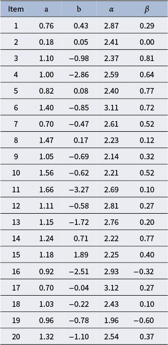
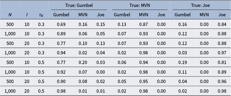


 Open access

