


1. Introduction
Ruin theory is concerned with the study of level crossing probabilities of certain stochastic processes with jumps. This is of clear interest in insurance, for example, where the focus is on the probability that the wealth process of a given insurance company reaches a lower level, in particular the level 0: in this case, the jumps represent claim sizes. There are also applications in storage, for example of water in a dam: in that context, the jumps represent water arrival events, such as rainfalls. The probability that the water level reaches critical levels for the dam is important for energy management, for instance. We refer the reader to the monograph [Reference Asmussen and Albrecher3] for further details on applications of ruin theory to other problems, in particular its duality with queuing theory.
In this paper, we use the terminology and interpretations from insurance. Let τ 1,τ 2,… be a sequence of positive random variables on a probability space (Ω, ℱ, ℙ) and let Tn ≔ τn − τn−1 (τ0 ≔ 0). Now define
 $${N_t}{\kern 1pt} : = \# \{ n \ge 1:{\kern 1pt} {\tau _n} \le t\} ,\quad \quad t \ge 0,$$
the counting process associated with the sequence (τn)n ≥0. This last sequence represents the arrival epochs of the claims, and Nt is the number of claims in the time interval [0, t].
Let (ξi)i≥0 be an independent and identically distributed (i.i.d.) sequence of nonnegative random variables, defined on the same probability space, with finite second moments, i.e. satisfying  ${\mathbb{E}}(\xi _i^2) \lt \infty $. Moreover suppose that the sequence (ξi)i≥0 is independent of the process N. The aggregate claim size up to time t is given by
 $\sum\nolimits_{i = 1}^{{N_t}} {\xi _i}$. We assume that the insurer receives premia from customers at a rate c ∈ ℝ+. The claim surplus process is defined by
 ${S_t} = \sum\nolimits_{i = 1}^{{N_t}} {\xi _i} - ct$ and the risk reserve process by
 $${R_t} = x - {S_t} = x + ct - \sum\limits_{i = 1}^{{N_t}} {\xi _i},\quad \quad t \in [0,\infty ),$$
where x ∈ [0, ∞) is the initial reserve. Within the ruin model the insurer’s vulnerability to financial distress is measured in terms of the ruin probability up to a given time horizon T ∈ (0, ∞):
 $$\rho (x,T){\kern 1pt} : = (\mathop {\inf }\limits_{t \in [0,T]} {R_t} \lt 0).$$
De Vylder and Goovaerts [Reference Vylder and Goovaerts14] suggested the following modification of the risk reserve process:
 $${\tilde{R}}{\kern 1pt} : = x - {{\tilde{S}}_t}{\kern 1pt} : = x + ct - {{{N_t}} \over {{N_T}}}\sum\limits_{i = 1}^{{N_T}} {\xi _i},$$
with the convention that if N T = 0, then  $({N_t}/{N_T})\sum\nolimits_{i = 1}^{{N_T}} {\xi _i} = 0$, too. The ruin probability is given in that case by
 $$\tilde\rho (x,T){\kern 1pt} : = {\mathbb{P}}(\mathop {\inf }\limits_{t \in [0,T]} {{\tilde{R}}_t} \lt 0).$$
The processes R and  ${\tilde{R}}$ have the same jump times and the same values at times 0 and T, but the jump sizes of
 ${\tilde{R}}$ are equalized, in the sense that each jump of
 ${\tilde{R}}$ is equal to the average jump of R between times 0 and T.
The De Vylder and Goovaerts conjecture can then be stated as follows.
Open problem 1.1. For all x ≥ 0 and all T > 0,
 $${\tilde{\rho}} (x,T) \le \rho (x,T).$$
Define
 $${\rho _n}(x,T){\kern 1pt} : = {\mathbb{P}}(\mathop {\inf }\limits_{t \in [0,T]} {R_t} \lt 0|{N_T} = n),\quad \quad n \ge 0.$$
As explained in [Reference Vylder and Goovaerts14], (1.3) is equivalent to the fact that  ${{\tilde{\rho}} _n}(x,T) \le {\rho _n}(x,T)$, for every n ≥ 0, where
 ${{\tilde{\rho}} _n}$ is defined as ρ n, with
 ${\tilde{R}}$ R instead of R. Obviously,
 ${{\tilde{\rho}} _0}(x,T) = {\rho _0}(x,T)$. It is proved in [Reference Vylder and Goovaerts14] that
 ${{\tilde{\rho}} _1}(x,T) = {\rho _1}(x,T),{\rm{ }}{{\tilde{\rho}} _2}(x,T) \le {\rho _2}(x,T)$, and that the probabilities coincide in the case of an initial reserve equal to zero,
 ${\tilde{\rho}} (0,T) = \rho (0,T)$, but the general case has yet to be established. The results in [Reference Vylder and Goovaerts14] are derived analytically, using polynomial representations for the ruin probabilities.
Progress towards a proof of (1.3) was made in [Reference Robert12], where it is proved, using stop-loss order techniques, that for each u ≥ 0,
 $$\int_u^{ + \infty } \tilde \rho (x,T){\rm{d}}x \le \int_u^{ + \infty } \rho (x,T){\kern 1pt} {\rm{d}}x.$$
We are not aware of any further articles providing results on Problem 1.1.
Our idea is to approximate both processes (S t)t∈[0,T] and  ${({{\tilde{S}}_t})_{t \in [0,T]}}$ with continuous diffusions. Standard references for these type of approximations, using functional limit theorems, include in particular [Reference Asmussen2], [Reference Furrer, Michna and Weron7], [Reference Grandell8], and [Reference Iglehart9]. The idea is to rescale both time and space, time in order to let the number of claims increase and space in order to make the claim sizes smaller so that the risk reserve process converges in distribution to a continuous process.
It is well known that the surplus process (S t)t∈[0,T] can be approximated with a Brownian motion with drift (see e.g. Chapter V in [Reference Asmussen and Albrecher3]). We show also that  ${({{\tilde{S}}_t})_{t \in [0,T]}}$ has a diffusion approximation. Conditional to the terminal value at time T, both diffusion approximations are Brownian bridges. The diffusion rate of the Brownian bridge approximating (S t)t∈[0,T] is greater than or equal to the diffusion rate of the Brownian bridge approximating
 ${({{\tilde{S}}_t})_{t \in [0,T]}}$. Since the probability for a Brownian bridge to hit zero is increasing in the diffusion rate, the ruin probability for the first diffusion approximation is larger than for the second. The De Vylder–Goovaerts conjecture is therefore true for the diffusion limits.
We consider two cases for computing the diffusion limits. In the first case we assume that c = λ𝔼(ξ 1). In this case the accumulated premia coincide with the expected aggregate claims. In Section 2, we derive the diffusion limits by scaling time with a factor m while scaling the aggregate claim size with  $1/\sqrt m $, and we also characterize the distribution of the limit as the solution of a stochastic differential equation. In the second case, which is dealt with in Section 3, we assume that c exceeds λ𝔼(ξ 1). The difference η ≔ c − λ𝔼(ξ 1) is usually referred to as the safety loading. We compute the diffusion limits by scaling time with 1/η 2 and letting η ↓ 0, which is referred to as the heavy traffic approximation in risk theory ([Reference Asmussen and Albrecher3]).
2. Zero safety loading
To deal with diffusion approximations, we introduce D[0, T], the space of real càdlàg functions on [0,T], i.e. the real functions that are right-continuous and have left-hand limits. We next recall the definition of weak convergence on this space.
We say that a sequence of càdlàg processes (X n) converges in distribution to the càdlàg process X if, for every bounded function f : D[0, T] → ℝ that is continuous with respect to the Skorokhod topology (see e.g. [Reference Billingsley5]), we have
 $${\mathbb{E}}(\,f({X_n})) \to {\mathbb{E}}(\,f(X)).$$
We make the following assumption on the inter-arrival claim times.
Assumption 2.1. There exist positive constants ν and κ such that the process
 $${({1 \over {\kappa \sqrt n }}\sum\limits_{j = 1}^{nt} ({T_j} - \nu ))_{t \in [0,T]}}$$
converges in distribution in D[0, T] to a standard Brownian motion as n →∞.
Using the central limit theorem, we know that Assumption 2.1 is satisfied if the random variables (T n)n≥1 are independent and identically distributed with mean ν and variance κ 2. This is the so-called renewal theory framework. In the particular case where the common distribution of the variables (T n)n≥1 is exponential, N is a Poisson process, and the model defined in (1.1) is the so-called Cramér–Lundberg model. By analogy with the Poisson case, we write λ ≔ 1/ν.
Assumption 2.1 implies the convergence (Theorem 14.6 in [Reference Billingsley5])
 $${({{{N_{tn}} - \lambda tn} \over {\kappa {\lambda ^{3/2}}\sqrt n }})_{t \in [0,T]}} \Rightarrow {({B_t})_{t \in [0,T]}},$$
where here, and for the remainder of the paper, ⇒ denotes convergence in distribution on D ≔ D([0, T)] and B is a Brownian motion.
Throughout this section we assume that c = λ𝔼(ξ 1). Note that this implies that in the compound Poisson case, the process (S t)t∈[0, T] is a martingale.
We first characterize the laws of the diffusion limits of (S t)t∈[0, T] and  ${({{\tilde{S}}_t})_{t \in [0,T]}}$ with the help of a Brownian motion. Let V( · ) denote the variance operator. We introduce the constants
 $$\gamma {\kern 1pt} : = \sqrt {\lambda V({\xi _1}) + {\lambda ^3}{\kappa ^2}{\mathbb{E}}{{[{\xi _1}]}^2}} ,$$
 $$\sigma {\kern 1pt} : = \kappa {\lambda ^{3/2}}{\kern 1pt} {\mathbb{E}}({\xi _1}).$$
Note that γ ≥ σ, and that equality is satisfied if and only if the claims ξ i are deterministic.
2.1. Limiting diffusions
Proposition 2.1. The process (m −1/2 Stm)t∈[0, T] converges in law on D[0, T] to
 $${U_t}{\kern 1pt} : = \gamma {B_t},\quad \quad t \in [0,T],$$
as m →∞.
In the proof of Proposition 2.1 we make use of the continuous mapping theorem, which, for the ease of the reader, we recall here.
Proposition 2.2. (For example Theorem 2.7 in [Reference Billingsley5].) Let M and M′ be two metric spaces, h : M → M′ a measurable mapping and let Dh denote the set of discontinuities of h. Let (X n) be an M-valued sequence of random variables converging to a random variable X in distribution as n →∞. If ℙ(X ∈ D h) = 0, then h(X n) converges to h(X) in distribution as n →∞.
Proof of Proposition 2.1. Let us write
 $${1 \over {\sqrt m }}{S_{tm}} = {1 \over {\sqrt m }}\sum\limits_{i = 1}^{{N_{tm}}} ({\xi _i} - {\mathbb{E}}[{\xi _1}]) + {1 \over {\sqrt m }}{\mathbb{E}}[{\xi _1}]({N_{tm}} - \lambda tm).$$
Define
 $${Z_m}(t){\kern 1pt} : = {1 \over {\sqrt m }}\sum\limits_{j = 1}^{tm} ({\xi _j} - {\mathbb{E}}[{\xi _1}]).$$
By Donsker’s theorem,
 $${({1 \over {\sqrt {V({\xi _1})} }}{Z_m}(t))_{t \in [0,T]}}$$
converges in distribution on D,as m goes to +∞, to a Brownian motion. On the other hand, (2.1) entails that
 $${({1 \over {\sqrt m }}{\mathbb{E}}[{\xi _1}]({N_{tm}} - \lambda tm))_{t \in [0,T]}} \Rightarrow {(\sigma {B_t})_{t \in [0,T]}}.$$
Let W be a Brownian motion that is independent of B. By independence of N and the sequence (ξ m)m ≥ 1, the pair of scaled processes
 $${({Z_m}(t),{1 \over {\sqrt m }}{\mathbb{E}}[{\xi _1}]({N_{tm}} - \lambda tm))_{t \in [0,T]}}$$
converges in distribution to  ${(\sqrt {V({\xi _1})} {W_t},\sigma {B_t})_{t \in [0,T]}}$.
Since N tm/m converges in distribution on D to the function Φ : t ↦ λt, this implies, using Theorem 3.9 in [Reference Billingsley5], that
 $${({{{N_{tm}}} \over m},{Z_m}(t),{1 \over {\sqrt m }}{\mathbb{E}}[{\xi _1}]({N_{tm}} - \lambda tm))_{t \in [0,T]}} \Rightarrow {(\lambda t,\sqrt {V({\xi _1})} {W_t},\sigma {B_t})_{t \in [0,T]}}.$$
Let D 0 be the space of nondecreasing functions in D. As the function Φ is continuous and strictly increasing, we can use Theorem 3.1 in [Reference Whitt15] to obtain that the mapping defined on D 0 × D by (y, x) ↦ x ↦ y is continuous at (Φ, x′ ) for arbitrary x′ ∈ D. Consequently, Ψ : D 0 × D 2 → D 2, given by Ψ (y, x, z) = (x ↦ y, z), is continuous at (Φ, x′, z′) for arbitrary x′, z′ ∈ D. The continuous mapping theorem now implies
 $${({Z_m}({{{N_{tm}}} \over m}),{1 \over {\sqrt m }}{\mathbb{E}}[{\xi _1}]({N_{tm}} - \lambda tm))_{t \in [0,T]}} \Rightarrow (\sqrt {\lambda V({\xi _1})} {W_t},\sigma {B_t}{))_{t \in [0,T]}}.$$
By Theorem 4.1 in [Reference Whitt15], the addition of two elements in D is continuous at every (x, y), where x and y are continuous functions. By applying the continuous mapping theorem to the sum of the components in (2.4)we arrive at 1
 $${1 \over {\sqrt m }}{S_{tm}} \Rightarrow {(\sigma {B_t} + \sqrt {\lambda V({\xi _1})} {W_t})_{t \in [0,T]}}.$$
This last limit process is centred, Gaussian, and has the same covariance structure as the centred Gaussian process γ B, which ends the proof.
We now approximate  ${({{\tilde{S}}_t})_{t \ge 0}}$. Note that
 $${\mathbb{E}}[{{{N_t}} \over {{N_T}}}\sum\limits_{i = 1}^{{N_T}} {\xi _i}] = \lambda {\mathbb{E}}({\xi _1})t.$$
Hence  ${\mathbb{E}}({{\tilde{S}}_t}) = 0$ for all t ∈ [0, T].
Theorem 2.1. The scaled process  ${({m^{ - 1/2}}{\kern 1pt} {{\tilde{S}}_{tm}})_{t \in [0,T]}}$ converges in law on D[0, T] to
 $${{\tilde{U}}_t}{\kern 1pt} : = \sigma {B_t} + (\gamma - \sigma ){t \over T}{B_T},\quad \quad t \in [0,T],$$
as m →∞.
Proof. First we note that the process  ${\tilde{U}}$ is a centred Gaussian process with covariance function given by
 $$K(s,t) = ({\gamma ^2} - {\sigma ^2}){{st} \over T} + {\sigma ^2}(s \wedge t),\quad \quad s,t \in [0,T].$$
Consider the decomposition
 $${1 \over {\sqrt m }}{{\tilde{S}}_{tm}} = {1 \over {\sqrt m }}{{{N_{tm}}} \over {{N_{Tm}}}}\sum\limits_{i = 1}^{{N_{Tm}}} ({\xi _i} - {\mathbb{E}}[{\xi _1}]) + {1 \over {\sqrt m }} {\mathbb{E}}[{\xi _1}]({N_{tm}} - \lambda tm).$$
Define
 $${Z_m}(t){\kern 1pt} : = {1 \over {\sqrt m }}\sum\limits_{j = 1}^{tm} ({\xi _j} - {\mathbb{E}}[{\xi _1}]).$$
Now, notice that the decomposition (2.7) can be written as
 $${1 \over {\sqrt m }}{{\tilde{S}}_{tm}} = {{{N_{tm}}} \over {{N_{Tm}}}}{Z_m}({{{N_{Tm}}} \over m}) + {1 \over {\sqrt m }}{\mathbb{E}}[{\xi _1}]({N_{tm}} - \lambda tm).$$
The quantity N tm/N Tm (resp. N Tm/m) converges in distribution on D to t ↦ t/T (resp. t ↦ λT).
Theorem 3.9 of Billingsley [Reference Billingsley5] implies that
 $${({{{N_{Tm}}} \over m},{{{N_{tm}}} \over {{N_{Tm}}}},{Z_m}(t),{1 \over {\sqrt m }}{\mathbb{E}}[{\xi _1}]({N_{tm}} - \lambda tm))_{t \in [0,T]}} \Rightarrow {(\lambda T,{t \over T},\sqrt {V({\xi _1})} {W_t},\sigma {B_t})_{t \in [0,T]}}black.$$
By Theorems 3.1, 4.2, and 4.1 in [Reference Whitt15] the mapping h : D × D 0 × D 2 → D, (x′, y′, z′, v′) ↦ x′ (z′ ↦ y′ ) + v′, is continuous at every quadruple of continuous functions (x, y, z, v) with y being strictly increasing. The continuous mapping theorem, applied to h and the convergent sequence (2.8), yields
 $${1 \over {\sqrt m }}{{\tilde{S}}_{tm}} \Rightarrow {t \over T}\sqrt {\lambda V({\xi _1})} {W_T} + \sigma {B_t} = :{\kern 1pt} {V_t}.$$
Here V and  ${\tilde{U}}$ are centred Gaussian processes with the same covariance function given in (2.6), so they have the same distribution, and the proof is complete.☐
We briefly comment on the method we use for proving Proposition 2.1 and Theorem 2.1. Recall that a more commonly used method for proving convergence in distribution on D is, first, to prove weak convergence of finite-dimensional distributions and, second, to show tightness of the considered sequence of probability measures on D (see e.g. Section 13 in [Reference Billingsley5]). A convenient method for verifying tightness is to show that the second moment, or another appropriately chosen moment, of the product of two neighbouring process increments can be nicely controlled.
This commonly used approach can also be applied to the two scaled process families of Proposition 2.1 and Theorem 2.1, respectively. A sufficient moment criterion for tightness of the distributions of (m −1/2 S ·m), m ≥ 1, is that there exists a constant C ∈ [0, ∞) such that, for all r, s, t ∈ [0, T] with r ≤ s ≤ t, we have
 $${\mathbb{E}}[({S_s} - {S_r}{)^2}{({S_t} - {S_s})^2}] \le C{(t - r)^2}$$
(see e.g. Section 13 in [Reference Billingsley5]). The same moment criterion applies to the scaled versions of  $\tilde S$. Note that the increments of (S t)t∈[0, T] and
 ${({\tilde S_t})_{t \in [0,T]}}$ are not independent. Even in the Poisson case where (S t)t∈[0, T] has independent increments, the increments of
 $\tilde S$ are not independent. The dependence of increments implies that the moment criterion for verifying tightness requires a stronger integrability condition on the claim sizes (ξ i)i≥1 than L 2-integrability.
The approach that we follow for proving Proposition 2.1 and Theorem 2.1 requires only L 2-integrability of the claim sizes. The reason is that it falls back on limit theorems for simpler processes and then applies the continuous mapping theorem for the Skorokhod topology. This approach relies on results of [Reference Whitt15], and it has been used in particular in [Reference Furrer, Michna and Weron7] in the context of diffusion approximations of risk processes.
Remark 2.1. Let z ∈ D([0, T]) be a given path with finite jump activity, i.e. such that z admits a finite number of jumps in any finite interval (notice that S and  ${\tilde{S}}$ have finite jump activity, almost surely). Then define n t(z) as the number of jumps of z during the time interval [0, t]. The path z can always be written as
 $$z(t) = {z_c}(t) + \sum\limits_{0 \lt t \le T} (z(t) - z({t^ - })),$$
where z c is a continuous trajectory and z(t −) is the left-hand side limit of z at t.The transformation suggested by De Vylder and Goovaerts is the application R: D → D,
 $$R(z)(t){\kern 1pt} : = {z_c}(t) + {n_t}(z)({1 \over {{n_T}(z)}}\sum\limits_{0 \lt t \le T} (z(t) - z({t^ - }))),$$
that replaces each jump of z by the average jump of z between 0 and T.
A simple consequence of our results is that the application R is not continuous for the Skorokhod topology. If it were, then Proposition 2.1 would imply that
 $$R({1 \over {\sqrt m }}{S_{ \cdot m}}) = {1 \over {\sqrt m }}{{\tilde{S}}_{ \cdot m}}$$
converges in distribution on D for the Skorokhod topology to R(γ B) = γ B, which is not the case, by Theorem 2.1.
2.2. Comparison of the ruin probabilities
Let X t ≔ x − U t and 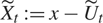 ${{\tilde{X}}_t}{\kern 1pt} : = x - {{\tilde{U}}_t}$. The ruin probability ρ can be approximated by χ ≔ ℙ(inft∈[0, T] X t < 0) and the ruin probability
 ${\tilde{\rho}}{\rm{by}}{\tilde{\chi}} {\kern 1pt} : = {\mathbb{P}}(\mathop {\inf }\nolimits_{t \in [0,T]} {{\tilde{X}}_t} \lt 0)$. In this section we show that
 ${\tilde{\chi}} \le \chi $.
First note that  ${X_T} = {{\tilde{X}}_T}$. Conditional to X T = y, the process (X t)t∈[0, T] is a Brownian bridge from x to y with diffusion rate γ. We can therefore derive an explicit formula for the conditional probability that (X t)t∈[0, T] goes below zero at some time before T.
To make this precise, let B be the collection of Borel sets on the space of continuous functions C([0, T]) endowed with the supremum norm. Moreover, let ℬ × ℝ ∍(A, y) ↦ ℙ(A|X T = y) be a regular conditional distribution of (X t)t∈[0, T] with respect to X T.
Lemma 2.1. For all y ≥ 0 we have
 $${\mathbb{P}}(\mathop {\inf }\limits_{t \in [0,T]} {X_t} \lt 0|{X_T} = y) = \exp ( - 2{{xy} \over {T{\gamma ^2}}}).$$
Proof. One can show ([Reference Revuz and Yor11, Chapter I]) that the law of (X t)t∈[0, T] under ℙ(·|X T = y) coincides with the law for a Brownian bridge from x to y with diffusion rate γ. Therefore,
 $${\mathbb{P}}(\mathop {\inf }\limits_{t \in [0,T]} {X_t} \lt 0|{X_T} = y) = {\mathbb{P}}(\mathop {\inf }\limits_{t \in [0,{\gamma ^2}T]} {B_t} \lt - x|{B_{{\gamma ^2}T}} = y - x).$$
Well-known results on hitting probabilities for Brownian bridges (see e.g. Proposition 3 in [Reference Scheike13]) imply the result.☐
We next derive an explicit formula for the conditional probability that  ${\tilde{X}}$ goes below zero at some time before T. To this end, recall that the process
 $${Y_t}{\kern 1pt} : = ({B_t} - {t \over T}{B_T}),\quad \quad t \in [0,T],$$
is a Brownian bridge on [0, T] from zero to zero. Observe that
 $${{\tilde{U}}_t} = \sigma {Y_t} + \gamma {t \over T}{B_T} = \sigma {Y_t} + {t \over T}(x - {X_T}),$$
and that B T is independent of Y t. Conditional to X T = y, the process  ${({{\tilde{X}}_t})_{t \in [0,T]}}$ is therefore a Brownian bridge from zero to y with diffusion rate σ. From well-known results on hitting probabilities of Brownian bridges, we arrive at the following result.
Lemma 2.2. For all y ≥ 0 we have
 $${\mathbb{P}}(\mathop {\inf }\limits_{t \in [0,T]} {{\tilde{X}}_t} \lt 0|{X_T} = y) = \exp ( - 2{{xy} \over {T{\sigma ^2}}}).$$
Lemmas 2.1 and 2.2 imply that the difference of ruin probabilities χ and  ${\tilde{\chi}} $ satisfies
 $$\matrix{
{\chi - {\tilde{\chi}} } & = & {\int_0^\infty [{\mathbb{P}}(\mathop {\inf }\limits_{t \in [0,T]} {X_t} \lt 0|{X_T} = y) - {\mathbb{P}}(\mathop {\inf }\limits_{t \in [0,T]} {{{\tilde{X}}}_t} \lt 0|{X_T} = y)]{\mathbb{P}}({X_T} \in {\kern 1pt} {\rm{d}}y)} \cr
{} & = & {\int_0^\infty [\exp ( - 2{{xy} \over {T{\gamma ^2}}}) - \exp ( - 2{{xy} \over {T{\sigma ^2}}})]{1 \over {\sqrt {2\pi {\gamma ^2}T} }}\exp ( - {{{{(y - x)}^2}} \over {2{\gamma ^2}T}}){\kern 1pt} {\rm{d}}y} \cr
{} & \ge & {0.} \cr
} $$
Note that the difference is greater than zero if γ > σ. Thus we have obtained the following result.
Theorem 2.2. It holds that
 $${\mathbb{P}}(\mathop {\inf }\limits_{t \in [0,T]} {{\tilde{X}}_t} \lt 0) \le {\mathbb{P}}(\mathop {\inf }\limits_{t \in [0,T]} {X_t} \lt 0),$$
where we have equality if and only if the claim sizes (ξ i)i≥0 are deterministic.
Remark 2.2. The assumption made on the counting process N in the formulation of De Vylder and Goovaerts [Reference Vylder and Goovaerts14] differs from our Assumption 2.1. In [Reference Vylder and Goovaerts14], it is assumed that N is a homogeneous risk process, meaning that conditionally on (N T = n), the vector of jump times (τ 1,…,τn) has the same distribution as the increasing order statistics of n independent uniform random variables on [0, T]. In particular, this property is satisfied when N is a Poisson process. More details and properties of the homogeneous process are given in [Reference Lefèvre and Picard10]. If we assume that (N t)t∈ℝ+ is a homogeneous process, then according to Theorem A2 in [Reference Vylder and Goovaerts14], it is a mixed Poisson process. This entails, using the same lines of reasoning as in Chapter 4 of [Reference Furrer6] (pages 65–67), that our limit results hold, with λ replaced by a structure random variable Λ. Then, by conditioning on this variable, we can still compare the ruin probabilities in the diffusion limits, as in the previous theorem.
Remark 2.3. All the results presented so far remain true if we omit the assumption that each random variable ξ i is nonnegative but simply assume that E(ξ i) ≥ 0.
2.3. The dynamics of the approximating diffusion
We close this section by characterizing  ${({{\tilde{U}}_t})_{t \in [0,T]}}$, the diffusion limit of the claim surplus process within the model with equalized claims, as a solution of a stochastic differential equation (SDE). First observe that the diffusion limit
 ${({{\tilde{U}}_t})_{t \in [0,T]}}$ is a Gaussian process. Recall that the law of a one-dimensional Gaussian process (Z t)t∈[0, T] is uniquely determined by its expectation function m(t) ≔ 𝔼(Z t) and covariance function K(t, s) ≔ Cov(Z t, Z s). Hence, we can characterize the limiting law of
 ${({m^{ - 1/2}}{\kern 1pt} {{\tilde{S}}_{tm}})_{t \in [0,T]}}$ as that of a Gaussian process with m(t) = 0 and
 $$K(s,t) = ({\gamma ^2} - {\sigma ^2}){{st} \over T} + {\sigma ^2}(s \wedge t)\quad {\rm{for \ s,t}} \in {\rm{[0,T],}}$$
where the constants γ and σ are defined in (2.2) and (2.3). This also allows us to characterize the limiting law in terms of an SDE.
Proposition 2.3. There exists a Brownian motion  ${({{\tilde{W}}_t})_{t \in [0,T]}}$ such that the process
 $({{\tilde{U}}_t})$ satisfies
 $${\rm{d}}{{\tilde{U}}_t} = {{\tilde{U}}_t}{{{\gamma ^2} - {\sigma ^2}} \over {{\sigma ^2}(T - t) + {\gamma ^2}t}}{\kern 1pt} {\rm{d}}t + \sigma {\kern 1pt} {\rm{d}}{{\tilde{W}}_t}$$
on [0, T].
Proof. We first solve explicitly the SDE (2.10) for a given Brownian motion (W t)t∈[0, T]. To this end, let
 $$f(t) = {{{\gamma ^2} - {\sigma ^2}} \over {{\sigma ^2}(T - t) + {\gamma ^2}t}}\quad {\rm{for \ all}} \ t \in {\rm{[0,T]}}{\rm{.}}$$
Note that the SDE dZ t = Z tf (t) dt + σ dW t with initial condition Z 0 = 0 has a unique solution given by
 $${Z_t} = \int_0^t \exp (\int_s^t f(u){\kern 1pt} {\rm{d}}u)\sigma {\kern 1pt} {\rm{d}}{W_s},\quad \quad t \in [0,T].$$
The solution process (Z t)t∈[0, T] is a Gaussian process. The covariance structure of (Z t)t∈[0,T] coincides with that of  ${({{\tilde{U}}_t})_{t \in [0,T]}}$. Indeed, for any s, t ∈ [0, T], the Itô isometry implies
 $${\rm{Cov}}({Z_s},{Z_t}) = \int_0^{s \wedge t} \exp (\int_r^s f(u){\rm{d}}u)\exp (\int_r^t f(u){\kern 1pt} {\rm{d}}u){\sigma ^2}{\kern 1pt} {\rm{d}}r.$$
Note that exp
 $$\exp (\int_r^k f(u){\kern 1pt} {\rm{d}}u) = {{{\sigma ^2}T + ({\gamma ^2} - {\sigma ^2})k} \over {{\sigma ^2}T + ({\gamma ^2} - {\sigma ^2})r}}\quad {\rm{for \ any}}k \in {\rm{[r,T]}}{\rm{.}}$$
Now a straightforward computation shows that
 $${\rm{Cov}}({Z_s},{Z_t}) = {\sigma ^2}(s \wedge t) + ({\gamma ^2} - {\sigma ^2}){{st} \over T}.$$
As a consequence, the process (Z t)t∈[0, T] has the same law as the process  ${({{\tilde{U}}_t})_{t \in [0,T]}}$. Now define
 $${{\tilde{W}}_t}{\kern 1pt} : = {1 \over \sigma }({{\tilde{U}}_t} - \int_0^t {{\tilde{U}}_s}f(s){\rm{ d}}s).$$
Then the pair 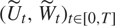 ${({{\tilde{U}}_t},{{\tilde{W}}_t})_{t \in [0,T]}}$ has the same process distribution as (Z t, W t)t∈[0, T]. In particular,
 ${({{\tilde{W}}_t})_{t \in [0,T]}}$ is a Brownian motion and
 ${({{\tilde{U}}_t})_{t \in [0,T]}}$ satisfies (2.10).
Remark 2.4. The dynamics (2.10) can be derived from (2.5) via a projection argument. To explain this, let  ${({\widetilde{\cal F}_t})_{t \in [0,T]}}$ be the smallest filtration such that, first, the usual conditions of right-continuity and completeness are satisfied and, second,
 ${({{\tilde{U}}_t})_{t \in [0,T]}}$ is adapted. Denote by
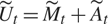 ${{\tilde{U}}_t} = {{\tilde{M}}_t} + {{\tilde{A}}_t}$ the Doob–Meyer decomposition of
 ${({{\tilde{U}}_t})_{t \in [0,T]}}$ with respect to
 ${({\widetilde{\cal F}_t})_{t \in [0,T]}}$. Assume that there exists an integrable
 $({\widetilde{\cal F}_t})$-predictable process α such that
 ${{\tilde{A}}_t} = \int_0^t {\alpha _s}{\kern 1pt} {\rm{d}}s,{\rm{ }}t \in [0,T]$. Since
 ${\langle {\tilde{M}},{\tilde{M}}\rangle _t} = {\langle {\tilde{U}},{\tilde{U}}\rangle _t} = {\sigma ^2}t$, for all t ∈ [0, T], we conclude from Levy’s theorem that
 ${\tilde{M}}/\sigma $ is a Brownian motion with respect to
 $({\widetilde{\cal F}_t})$.
For the Brownian bridge Y, defined in (2.9), there exists a Brownian motion W Y such that
 $${\rm{d}}{Y_t} = {\rm{d}}W_t^Y - {{{Y_t}} \over {T - t}}{\kern 1pt} {\rm{d}}t.$$
Since B T is independent of Y t, the process W Y is also a Brownian motion with respect to the initially enlarged filtration (𝒢 t), where  ${{\cal G}_t}{\kern 1pt} : = { \cap _{s > t}}({\cal F}_s^Y \vee \sigma ({B_T}))$. In particular,
 ${({{\tilde{X}}_t})_{t \in [0,T]}}$ is a (𝒢 t)-Itô process with dynamics
 $${\rm{d}}{{\tilde{U}}_t} = \gamma {1 \over T}{B_T}{\kern 1pt} {\rm{d}}t - {{\sigma {Y_t}} \over {T - t}}{\kern 1pt} {\rm{d}}t + \sigma {\kern 1pt} {\rm{d}}W_t^Y = {{\gamma {B_T} - {{{\tilde{U}}}_t}} \over {T - t}}{\kern 1pt} {\rm{d}}t + \sigma {\kern 1pt} {\rm{d}}W_t^Y.$$
Note that  $W_t^Y = {{\tilde{W}}_t} - \int_0^t {\mu _s}{\kern 1pt} {\rm{d}}s$, where
 $${\mu _t} = - {1 \over \sigma }({\alpha _t} - {{\gamma {B_T} - {{{\tilde{U}}}_t}} \over {T - t}}).$$
The process μ is the so-called information drift of  ${\tilde{W}}$ with respect to the enlarged filtration (𝒢 t). It is known that the L 2-projection of μ onto the space of square-integrable and
 $({\widetilde{\cal F}_t})$-progressively measurable processes vanishes (see e.g. Section 1 in [Reference Ankirchner, Dereich and Imkeller1]). This entails that
 $${\alpha _t} = {{\tilde{U}}_t}{{{\gamma ^2} - {\sigma ^2}} \over {{\sigma ^2}(T - t) + {\gamma ^2}t}},\quad \quad t \in [0,T],$$
and hence (2.10).
3. The conjecture in the heavy traffic approximation
We now assume that η = c − λ𝔼(ξ 1) > 0. By scaling time with 1/η 2 and letting η ↓ 0, the laws of the diffusion limits of (S t)t∈[0, T] and  ${({{\tilde{S}}_t})_{t \in [0,T]}}$ are given by the following proposition.
Proposition 3.1. The process 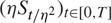 ${(\eta {S_{t/{\eta ^2}}})_{t \in [0,T]}}$ converges in law on D[0, T] to
 $${V_t}{\kern 1pt} : = \gamma {B_t} - t,\quad \quad t \in [0,T],$$
and the process 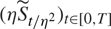 ${(\eta {{\tilde{S}}_{t/{\eta ^2}}})_{t \in [0,T]}}$ converges in law on D[0, T] to
 $${{\tilde{V}}_t}{\kern 1pt} : = \sigma {B_t} + (\gamma - \sigma ){t \over T}{B_T} - t,\quad \quad t \in [0,T],$$
as η → 0.
Proof. The proof is a straightforward adaptation of [3, Theorem 5.1] using the results from Proposition 2.1 and Theorem 2.1.
In the heavy traffic approximation, the ruin probability ρ can be approximated by
 $${\mathbb{P}}(\mathop {\sup }\limits_{t \in [0,T]} {V_t} \gt x)$$
and the ruin probability  ${\tilde{\rho}} $ by
 $${\mathbb{P}}(\mathop {\sup }\limits_{t \in [0,T]} {{\tilde{V}}_t} \gt x).$$
Following arguments similar to those of Section 2.2, we have  ${V_T} = {\tilde V_T}$, and the conditional nonruin probability is equal to
 $${\mathbb{P}}(\mathop {\sup }\limits_{t \in [0,T]} {V_t} \le x|{V_T} = y) = {\mathbb{P}}({B_t} \le {{x + t} \over \gamma },0 \le t \le T|{B_T} = {{y + T} \over \gamma }),\quad \quad y \lt x.$$
In other words, the nonruin probability conditional to V T = y is equal to the probability that a Brownian bridge starting form 0 and going to y/γ + T with length equal to T stays under the line t → (x + t)/γ. Using the results of [Reference Scheike13] and [Reference Atkinson and Singham4], we obtain
 $${\mathbb{P}}(\mathop {\sup }\limits_{t \in [0,T]} {V_t} \le x|{V_T} = y) = 1 - \exp ( - 2{{x(x - y)} \over {T{\gamma ^2}}}).$$
Using arguments similar to those of Section 2.2, it follows that
 $${\mathbb{P}}(\mathop {\sup }\limits_{t \in [0,T]} {{\tilde{V}}_t} \le x|{V_T} = y) = 1 - \exp ( - 2{{x(x - y)} \over {T{\sigma ^2}}}),$$
and hence we obtain that
 $${\mathbb{P}}(\mathop {\sup }\limits_{t \in [0,T]} {V_t} \le x|{V_T} = y) - {\mathbb{P}}(\mathop {\sup }\limits_{t \in [0,T]} {{\tilde{V}}_t} \le x|{V_T} = y) \le 0.$$
This implies that the De Vylder–Goovaerts conjecture holds in the heavy traffic approximation.
Acknowledgements
We thank an anonymous referee for valuable comments. S.A. gratefully acknowledges the hospitality and financial support of Ecole Centrale de Lyon during his visit in March 2018.


