



1. Introduction
Many real-world systems are both expensive and highly complex. As a result, system failures can lead to significant consequences. Therefore, a key challenge in reliability theory is determining how to extend the system’s lifetime. This issue is commonly addressed by incorporating one or more redundant components (spares) into the system. Redundancy allocation is an effective strategy for improving the lifetime of a system. Usually, two common methods of redundancy allocation are utilized to enhance the reliability of the system: active redundancy and standby redundancy. Active redundancy allocation involves assigning redundancy to a component so that both the original and redundant counterpart operate simultaneously. In contrast, standby redundancy allocation connects the redundancy such that it only activates when the original component fails. A significant amount of research has been done on these two allocations strategies.
The redundancy allocation methods discussed above may not always be feasible due to the possible increase in overall load and various economic considerations in certain scenarios [Reference Belzunce, Martínez and Ruiz10]. As an alternative, relevation allocation may be a more effective option than traditional active and standby redundancies. The concept of relevation was initially introduced by Krakowski [Reference Krakowski20]. The relevation model is commonly used in reliability engineering to describe the effectiveness of redundancy allocation in coherent systems. Its detailed mathematical definition is as follows: consider two non-negative independent random variables T and S having survival functions
 $ \overline{F}_{T} $
and
 $ \overline{F}_{S} $
, then the survival function of the relevation operation between T and S (denoted as
 $ T \# S $
) is given as [Reference Krakowski20]
 \begin{align} \overline{F}_{T \# S}(t) &=\overline{F}_{T}(t)+\overline{F}_{S}(t) \int_0^t \frac{1}{\overline{F}_{S}(x)} \, \mathrm{d} F_{T}(x), \quad \text{for}\; t>0. \end{align}
To understand this, let us consider two items with independent non-negative random lifetimes T and S. Once the item with lifetime T fails, it is replaced by another item with lifetime S such that it has the same age as that of the failed item. Then, the survival for the time until the second failure is represented by (1) [Reference Belzunce, Martnez, Mercader and Ruiz11, Reference Zhang and Zhang34]. Due to its practical significance, relevation is applied across a range of real-world situations. We give two examples for relevation allocation.
Example 1. In a car, a machine part fails after several months of operation. Rather than replacing the entire machine, a new part of the same age, made with upgraded materials, is installed. Though similar in function to the original, this new part follows a different lifetime distribution than the old one. Consequently, the machine’s overall distribution changes after the new part is installed. Thus, the lifetime of the machine can be represented by relevation transformation.
Example 2. In a heating, ventilation, and air conditioning (HVAC) system, a component such as a fan motor fails after prolonged use. Rather than replacing the entire HVAC unit, a new fan motor of the same age but made from more heat-resistant materials is installed. While similar in function to the original, this new part follows a different lifetime distribution from the old one. As a result, the distribution of the HVAC system changes after the new fan motor is installed.
Before describing the relevant works in the literature, let us first review some fundamental concepts and definitions related to coherent systems. A system is considered coherent if all components are relevant, and whenever a failed component is replaced by a good one, the system lifetime does not decrease [Reference Barlow and Proschan12]. Series, parallel, and k-out-of-n systems are examples of coherent systems. Consider a coherent system consisting of n independent components with structure function
 $\tau$
. Assume the components are labeled by the numbers
 $1,2, \ldots, n$
, and for each component i, its lifetime is denoted by
 $T_i,\ i=1, \ldots, n$
. A path set
 $\mathcal{P}$
is defined as a collection of components whose functioning can guarantee the functioning of the system, and a cut set
 $\mathcal{C}$
is defined as a collection of components whose failures cause the failure of the system. Specifically, a path set
 $\mathcal{P}$
is called a minimal path set if any of its proper subsets is not a path set, and a cut set
 $\mathcal{C}$
is called a minimal cut set if no proper subset is a cut set. According to Barlow and Proschan [Reference Barlow and Proschan5], the system lifetime can be expressed as
 \begin{align*}\tau(\boldsymbol{T})=\tau\left(T_1, \ldots, T_n\right)=\max _{\mathcal{P} \in \mathcal{A}} \min _{j \in \mathcal{P}} T_j=\min _{C \in S} \max _{j \in \mathcal{C}} T_j .\end{align*}
Suppose
 $\mathcal{A}$
denotes the class of all minimal path sets, and
 $\mathcal{S}$
denotes the class of all minimal cut sets. In addition, let
 $\mathcal{A}_i=\{\mathcal{I} \in \mathcal{A}, i \in \mathcal{I}\}$
be the collection of minimal path sets in which each minimal path set contains component i, and
 $\mathcal{S}_i=\{\mathcal{J} \in \mathcal{S}, i \in \mathcal{J}\}$
be the collection of minimal cut sets in which each minimal cut set contains component i. Then, for any two components i and j, their structural relationship can be classified into the following six types [Reference Wu, Ding, Zhang and Zhao30, Reference Zhang and Zhang34]:
-
(i)
 $\mathcal{A}_i=\mathcal{A}_j$
, i.e. components i and j are included in same minimal path sets;
-
(ii)
$\mathcal{S}_i=\mathcal{S}_j$
, i.e. components i and j are included in same minimal cut sets; -
(iii)
$\mathcal{A}_i \subseteq \mathcal{A}_j$
, i.e. the minimal path sets including component i is a subset of those including component j; -
(iv)
$\mathcal{S}_i \subseteq \mathcal{S}_j$
, i.e. the minimal cut sets including component i is a subset of those including component j; -
(v)
$\mathcal{A}_i$
and
$\mathcal{A}_j$
do not contain each other; -
(vi)
$\mathcal{S}_i$
and
$\mathcal{S}_j$
do not contain each other.


Zhang and Zhang [Reference Zhang and Zhang34, p. 5] mentioned, ‘It is worth noting that some of the above six settings might occur simultaneously’. In light of this, an example of a system structure that satisfies cases (i)–(vi) is as follows: consider an eight-component coherent system with component lifetimes
 $ T_{1}, T_{2}, \ldots, T_{8} $
, as depicted in Figure 1. It is easy to verify that
 $\mathcal{A}_1 = \{ \{1, 3, 4\} \}$
,
 $\mathcal{A}_2 = \{ \{2, 3, 4\} \}$
,
 $\mathcal{A}_3 = \{ \{1, 3, 4\}, \{2, 3, 4\} \}$
,
 $\mathcal{A}_4 = \{ \{1, 3, 4\}, \{2, 3, 4\} \}$
,
 $\mathcal{A}_5 =$
 $\{\{5, 6, 8\} \}$
,
 $\mathcal{A}_6 = \{ \{5, 6, 8\} \}$
,
 $\mathcal{A}_7 = \{ \{7, 8\} \}$
,
 $\mathcal{A}_8 = \{ \{7, 8\} \}, \{5, 6, 8\}\}$
,
 $\mathcal{S}_1 = \{ \{1, 2, 5, 7\},\ \{1, 2,$
 $6, 7\}, \{1, 2, 8\} \}$
,
 $\mathcal{S}_2 = \{ \{1, 2, 5, 7\}, \{1, 2, 6, 7\}, \{1, 2, 8\} \}$
,
 $\mathcal{S}_3 = \{ \{3, 5, 7\}, \{3, 6, 7\}, \{3, 8\} \}$
,
 $\mathcal{S}_4 = \{ \{4, 5, 7\}, \{4, 6, 7\}, \{4, 8\} \}$
,
 $\mathcal{S}_5 = \{ \{1, 2, 5, 7\}, \{3, 5, 7\}, \{4, 5, 7\} \}$
,
 $\mathcal{S}_6 = \{ \{1, 2, 6, 7\},$
 $\{3, 6, 7\}, \{4, 6, 7\} \}$
, and
 $\mathcal{S}_7 = \{ \{1, 2, 5, 7\}, \{1, 2, 6, 7\}, \{3, 5, 7\}, \{3, 6, 7\}, \{4, 5, 7\}, \{4, 6, 7\} \}$
,
 $\mathcal{S}_8 = \{ \{3, 8\}, \{4, 8\} \}$
. Here,
 $\mathcal{A}_1 = \{ \{1, 3, 4\} \}$
denotes the minimal path sets containing component 1,
 $\mathcal{S}_1 = \{ \{1, 2, 5, 7\}, \{1, 2, 6, 7\}, \{1, 2, 8\} \}$
denotes the minimal cut sets containing component 1, and so on. Observe that
 $\mathcal{A}_5 = \mathcal{A}_6$
,
 $\mathcal{S}_1 = \mathcal{S}_2$
,
 $\mathcal{A}_1 \subseteq \mathcal{A}_3$
,
 $\mathcal{S}_5 \subseteq \mathcal{S}_7$
, whereas
 $\mathcal{A}_1$
and
 $\mathcal{A}_2$
do not contain each other (i.e.
 $\mathcal{A}_1 \nsubseteq \mathcal{A}_2$
and
 $\mathcal{A}_2 \nsubseteq \mathcal{A}_1$
), and neither do
 $\mathcal{S}_1$
and
 $\mathcal{S}_2$
(i.e.
 $\mathcal{S}_2 \nsubseteq \mathcal{S}_3$
and
 $\mathcal{S}_3 \nsubseteq \mathcal{S}_2$
).
Schematic diagram of an eight-component system.

An intriguing decision problem for system design engineers is determining how to allocate a given number of redundant components to a coherent system to maximize the system’s overall lifetime. In this regard, a few studies have been presented that investigate the optimal allocation policy for one or two revelations to a coherent system. Belzunce et al. [Reference Belzunce, Martínez and Ruiz10] studied the optimal allocation policy for one relevation performed to a series (parallel) system and then generalized it to a coherent system by assuming that the components where relevation is performed share similar minimal path (minimal cut) sets (i.e. for the cases: (i)
 $\mathcal{A}_i=\mathcal{A}_j$
and (ii)
 $\mathcal{S}_i=\mathcal{S}_j$
, where
 $\mathcal{A}_i, \mathcal{A}_j, \mathcal{S}_i,\; \text{and}\; \mathcal{S}_j$
are as defined previously). For this purpose, the authors considered a series system with two components having lifetimes
 $T_1$
and
 $T_2$
. Suppose two relevations with lifetimes
 $S_1$
and
 $S_2$
are available, but due to the budget constraint, we can perform only one relevation at a time. Then, the authors demonstrated that if
 $T_1 \leq_{hr} T_2$
and
 $S_1 \geq_{hr} S_2$
, then
 $U_1 \geq_{st} U_2$
, where
 $U_1 = \min\{T_1 \# S_1, T_2\}$
with
 $U_2 = \min\{T_1, T_2 \# S_2\}$
. They further extended this result to the coherent system with n components and showed that for components i and j in common path sets, the relevation should be allocated to the component with the higher hazard rate. In contrast, for components i and j in common cut sets, the relevation should be allocated to the component with the higher reversed hazard rate. Later, Wu et al. [Reference Wu, Ding, Zhang and Zhao30] complemented the results of [Reference Belzunce, Martínez and Ruiz10] by considering one relevation allocation problem to a coherent system for cases (iii)–(vi), and compared system lifetimes in the sense of usual stochastic order. Further, under the scenario where there is no budget issue and both the relevations can be performed at the same time (i.e. two possible allocations policies: either
 $S_1$
is attached with
 $T_i$
and
 $S_2$
with
 $T_j$
, or
 $S_2$
is attached with
 $T_i$
and
 $S_1$
with
 $T_j$
), Yan et al. [Reference Yan, Zhang and Zhang31] studied the allocation of two relevations to a coherent system simultaneously. They extended the work of [Reference Belzunce, Martínez and Ruiz10] by applying two simultaneous relevations in a coherent system, under the condition that the components where relevation is allocated share similar minimal path sets, i.e. for case (i)
 $\mathcal{A}_i=\mathcal{A}_j$
. Recently, Zhang and Zhang [Reference Zhang and Zhang34] have studied the optimal allocation policy for two relevations to a coherent system for cases (iii)–(vi) in terms of minimal path sets and cut sets. They made the stochastic comparison of coherent systems in the sense of the usual stochastic order.
From the aforementioned discussion, we make the following observations:
-
(a) very little work has been done so far in the literature on relevation allocation to coherent systems;
-
(b) most of the works have established the usual stochastic order between system lifetimes;
-
(c) although the allocation of two relevations (performed one at a time) to a coherent system has garnered the attention of researchers for cases (i)–(vi) [Reference Belzunce, Martínez and Ruiz10, Reference Wu, Ding, Zhang and Zhao30], the same does not hold true for the situation when two relevations are allocated (both at the same time) to a coherent system [Reference Yan, Zhang and Zhang31, Reference Zhang and Zhang34].
In this study, we aim to address these gaps in the literature. With regards to observation (a), we establish results on the stochastic comparison of system lifetimes after allocating two relevations (one at a time and both simultaneously) to a coherent system. Next, to address observation (b), we stochastically compare system lifetimes with respect to hazard rate order after allocations of two relevations (performed one at a time) (see Theorems 1 and 2). By doing so, we extend the results of [Reference Belzunce, Martínez and Ruiz10] and also answer the call for future research on hazard rate order. Finally, with regards to observation (c), we note that stochastic comparison results were established in [Reference Zhang and Zhang34] in the case of two relevations (performed simultaneously) on the series system. Thus, in this study, we address the gap on two relevation allocations (performed simultaneously) to a series system (by adding some more sufficient conditions in the literature) and a coherent system for case (i)
 $\mathcal{A}_i=\mathcal{A}_j$
(see Theorems 3 and 4). In addition, by building on the result for two relevation allocation to a parallel system (performed simultaneously), we provide stochastic comparison results in the case of two relevations (performed simultaneously) on the coherent system for case (ii)
 $\mathcal{S}_i=\mathcal{S}_j$
, and also provide additional sets of sufficient conditions for cases (iii)
 $\mathcal{A}_i \subseteq \mathcal{A}_j$
, and (iv)
 $\mathcal{S}_i \subseteq \mathcal{S}_j$
(see Theorems 4–7 and 8). By obtaining new findings on two relevations allocations (performed one at a time or both at the same time), we not only extend the results of [Reference Belzunce, Martínez and Ruiz10, Reference Wu, Ding, Zhang and Zhao30], but also generalize the results of [Reference Zhang and Zhang34]. In particular, for cases (i)
 $\mathcal{A}_i=\mathcal{A}_j$
and (iii)
 $\mathcal{A}_i \subseteq \mathcal{A}_j$
, we provided additional sets of sufficient conditions to those obtained in [Reference Zhang and Zhang34], and we also addressed the conjecture in Theorem 2 of Zhang and Zhang [Reference Zhang and Zhang34] by employing our Theorem 6 and establishing the usual stochastic order for two relevations allocation (performed both at the same time) to a coherent system for case (iv)
 $\mathcal{S}_i \subseteq \mathcal{S}_j$
.
As an application of our main results, we study the optimal allocation policy for two minimal repairs (performed one at a time) in a series system and a coherent system for case (i)
 $\mathcal{A}_i=\mathcal{A}_j$
, and make the stochastic comparison in sense of hazard rate order (see Theorems 9 and 10). For the case of multiple minimal repairs, the majority of the results focused either on identical components or on the same number of minimal repairs performed to series and coherent systems (see, for example, [Reference Arriaza, Navarro and Suárez3, Reference Navarro, Arriaza and Suárez24, Reference Navarro and Fernández-Martnez25]). With this in mind, we concentrate on determining the optimal allocation policy for multiple minimal repairs (which may vary in number) on a single node (or component) within coherent systems composed of nonidentical components. To fill these gaps for multiple minimal repairs, we provide the results for coherent systems in cases (i)
 $\mathcal{A}_i=\mathcal{A}_j$
and (iii)
 $\mathcal{A}_i \subseteq \mathcal{A}_j$
by employing the result for a series system (see Theorems 11, 12, and 13). In summary, the key contributions of this paper are as follows.
-
• This work explores the optimal allocation policy for two relevation performed (one at a time and both at a time) to a series or parallel system and then later generalized to a general coherent system for cases (i)–(iv) in the sense of the usual stochastic order and the hazard rate order.
-
• We study the optimal allocation policy for two minimal repairs (performed one at a time) and multiple minimal repairs to a series system and a coherent system for cases (i)
$\mathcal{A}_i=\mathcal{A}_j$
and (iii)
$\mathcal{A}_i \subseteq \mathcal{A}_j$
in the sense of the usual stochastic order and the hazard rate order.


The rest of the paper is structured as follows. The next section introduces several definitions and lemmas that will be instrumental in proving our main results. In Section 3, we provide our main results. Specifically, we examine the allocation problems of relevations for one (or two) node (or nodes) in a coherent system with independent components to enhance the system’s reliability. We have established several results concerning the usual stochastic order and hazard rate order for a coherent system. Next, Section 4 presents an application of our results through a simulation-based study and an analysis of real data. In addition, we study the case of the minimal repair policy in detail (see Subsection 4.3). Finally, in Section 5 we conclude our study.
2. Preliminaries and auxiliary results
Let X and Y be non-negative independent random variables with distribution functions
 $F_{X}$
and
 $F_{Y}$
, density functions
 $f_{X}$
and
 $f_{Y}$
, and survival functions
 $\overline{F}_{X}$
and
 $\overline{F}_{Y}$
, respectively. Throughout the paper, all random variables under consideration are assumed to be mutually independent. Moreover, ‘increasing’ refers to ‘nondecreasing’, and ‘decreasing’ refers to ‘nonincreasing’. In addition,
 $X \overset{d}{=} Y$
denotes that X and Y are identically distributed.
We first present the definitions of some commonly used stochastic orders, which are employed in this study. Stochastic orders are well-known to be useful for comparing the random lifetimes of two systems.
Definition 1. A random variable X is said to be smaller than random variable Y in the:
-
(i) usual stochastic order (denoted by
$X \leq_{st} Y$
) if
$\overline{F}_{X}(t) \leq \overline{F}_{Y}(t)$
, for all
$t \in [0, \infty);$
-
(ii) hazard rate order (denoted by
$X \leq_{hr} Y$
) if
$\overline{F}_{Y}(t)/\overline{F}_{X}(t)$
is increasing in
$t \in [0, \infty)$
; -
(iii) reversed hazard rate order (denoted by
$X \leq_{rh} Y$
) if
${F}_{Y}(t)/{F}_{X}(t)$
is increasing in
$t \in [0, \infty)$
; -
(iv) likelihood ratio order (denoted by
$X \leq_{lr} Y$
) if
${f}_{Y}(t)/{f}_{X}(t)$
is increasing in
$t \in [0, \infty)$
.


For a more detailed discussion on stochastic orders, readers can consult [Reference Belzunce, Riquelme and Mulero7, Reference Muller and Stoyan23, Reference Shaked and Shanthikumar29]. The following diagram depicts the chain of implications among the aforementioned stochastic orders.

The article also requires the idea of totally positive (reverse regular) functions of order 2
 $(TP_2 (RR_2))$
. In the domain of statistical reliability theory, totally positive (reverse regular) functions of order 2
 $(TP_2 (RR_2))$
naturally emerge when analyzing the reliability of coherent systems. Karlin made substantial contributions to this field, laying its foundations within probability and statistical theory. In 1968, he authored a seminal book on the subject, which spurred numerous advancements. Karlin [Reference Karlin19] defined a
 $TP_2 (RR_2)$
function as follows.
Definition 2. Let
 $S_1$
and
 $S_2$
be two subsets of the real line
 $\mathbb{R}$
. A non-negative function
 $k\;:\; S_1 \times S_2 \rightarrow[0, \infty)$
is said to be
 $T P_2\left(R R_2\right)$
if, for
 $x_1 \leq x_2, y_1 \leq y_2 (x_i \in S_1 ;\; y_i \in S_2,\ i=1,2)$
,
 \begin{align*}k\left(x_1, y_1\right) k\left(x_2, y_2\right) \geq(\!\leq\!) k\left(x_1, y_2\right) k\left(x_2, y_1\right).\end{align*}
The following lemma is the improvement of Lemma 3(iii) of [Reference Ding and Li13], in which we show that condition
 $g_1(t) \geq g_2(t)$
is not needed to prove
 $({g(t)+g_1(t)})/({g(t)+g_2(t)})$
is increasing in
 $t>0$
.
Lemma 1. Suppose real functions
 $g_1$
,
 $g_2$
, and g such that
 $g_1(t)$
,
 $g_2(t) \geq 0$
, and
 $g(t) \geq 0$
for all
 $t > 0$
. If both
 ${g_1(t)}/{g_2(t)}$
and
 ${g(t)}/({g_2(t)-g_1(t)})$
are increasing in t, then
 $({g(t)+g_1(t)})/({g(t)+g_2(t)})$
is also increasing in
 $t>0$
.
Proof. The proof is given in the Appendix.
The following lemma is due to Misra and Naqvi [Reference Misra and Naqvi22], which is very useful for proving our main results.
Lemma 2. Let
 $h_i(x, \theta)\;:\;[0, \infty) \times[0, \infty) \rightarrow \mathbb{R}$
,
 $i=1,2$
, be a function and
 $g_i(\theta)$
,
 $i=1,2$
, be the Lebesgue probability distribution function of the random variable
 $\Theta_i,\ i=1, 2$
. Let
 \begin{align*}K(x)=\frac{\int_0^{\infty} h_2(x, \theta) \,\textrm{d} G_2(\theta)}{\int_0^{\infty} h_1(x, \theta), \,\textrm{d} G_1(\theta)}.\end{align*}
Now, we define the following two pairs of conditions for the positive function
 $h_i,\ i=1,2$
: (i)
 $h_1(x, \theta)$
or
 $h_2(x, \theta)$
is
 $T P_2$
in
 $(x, \theta) \in(0, \infty) \times(0, \infty)$
; (ii)
 ${h_2(x, \theta)}/{h_1(x, \theta)}$
increasing in
 $x \in(0, \infty)$
and
 $\theta \in(0, \infty)$
; (iii)
 $h_1(x, \theta)$
or
 $h_2(x, \theta)$
is
 $R R_2$
in
 $(x, \theta) \in(0, \infty) \times(0, \infty)$
; and (iv)
 ${h_2(x, \theta)}/{h_1(x, \theta)}$
decreasing in
 $x \in(0, \infty)$
and increasing in
 $\theta \in(0, \infty)$
.
Suppose that conditions (i) and (ii) ((iii) and (iv)) hold. Further, if any of the following three conditions hold:
-
(a)
$\Theta_1 \leq_{l r} \Theta_2$
; -
(b)
$\Theta_1 \leq_{h r} \Theta_2$
and
$h_1(x, \theta)$
or
$h_2(x, \theta)$
is increasing in
$\theta \in(0, \infty)$
; -
(c)
$\Theta_1 \leq_{r h} \Theta_2$
and
$h_1(x, \theta)$
or
$h_2(x, \theta)$
is decreasing in
$\theta \in(0, \infty)$
.


Then the function K(x) is increasing (decreasing) in
 $x \in(0, \infty)$
(or, equivalently,
 $\int_0^{\infty} h_i(x, \theta) g_i(\theta)\,\textrm{d} \theta $
is
 $TP_2 (RR_2)$
in
 $(i, x) \in\{1,2\} \times [0, \infty)$
).
3. Main results
In this section, we consider two 2-component series (parallel) systems and establish optimal allocations of two relevations to these two series (parallel) systems. Moreover, we also study the optimal allocation policy for a general coherent system in the sense of various stochastic orderings, for cases (i)–(iv).
3.1. Allocation of two relevations in cases: (i)
$\mathcal{A}_i=\mathcal{A}_j$
and (iii)
$\mathcal{A}_i \subseteq \mathcal{A}_j$


In this subsection, we discuss the optimal allocation policies of one and two relevations for a series system and later generalize them to a coherent system in the sense of usual stochastic order and hazard rate order, for the cases: (i)
 $\mathcal{A}_i=\mathcal{A}_j$
and (iii)
 $\mathcal{A}_i \subseteq \mathcal{A}_j$
.
Suppose that a series system has two components with lifetimes
 $T_{1}$
and
 $T_{2}$
, and two relevations are available having lifetimes
 $S_{1}$
and
 $S_{2}$
. However, due to time and budget issues, suppose one can perform only one relevation at a time to the series system. That is, we are interested in the comparison between
 $U_1=\min \left\{T_1 \# S_1, T_2\right\}$
and
 $U_2=\min \left\{T_1, T_2 \# S_2\right\}$
, where the distribution function, survival function, and density function of a random variable
 $U_{1}$
 $(U_{2})$
are
 $F_{U_{1}}$
 $(F_{U_{2}})$
,
 $\overline{F}_{U_{1}}$
 $(\overline{F}_{U_{2}})$
, and
 $f_{U_{1}}$
 $(f_{U_{2}})$
, respectively. Suppose that the component lifetimes and the available relevation lifetimes are mutually independent. Belzunce et al. [Reference Belzunce, Martínez and Ruiz10] proved that if
 $T_{1} \leq_{hr} T_{2}$
and
 $S_{1} \geq_{hr} S_{2}$
then
 $U_{1} \geq_{st} U_{2}$
. One natural question arises that under what sufficient conditions
 $U_{1} \geq_{st} U_{2}$
can be strengthened to
 $U_{1} \geq_{hr} U_{2}$
? To answer this question, we provide the following result on the optimal allocation policy of two relevations (performed one at a time) for hazard rate order in the series system.
Theorem 1. Let
 $U_1=\min \left\{T_1 \# S_1, T_2\right\}$
and
 $U_2=\min \left\{T_1, T_2 \# S_2\right\}$
. Suppose
 $S_{1} \geq_{hr} T_{1}$
or
 $S_{2} \geq_{hr} T_{2}$
. In addition, if
 $T_{1}$
 $\leq_{hr}$
 $(\!\geq_{hr}\!)$
 $T_{2}$
and
 $S_{1}$
 $\geq_{hr}$
 $(\!\leq_{hr}\!)$
 $S_{2}$
then
 $U_{1}$
 $\geq_{hr}$
 $(\!\leq_{hr}\!)$
 $U_{2}$
.
Proof. First, we prove that
 $U_1 \geq_{hr} U_{2}$
under the conditions ‘
 $S_{1} \geq_{hr} T_{1}$
’, ‘
 $T_{1} \leq_{hr} T_{2}$
’, and ‘
 $S_{1} \geq_{hr} S_{2}$
’. To prove
 $U_1 \geq_{hr} U_{2}$
, it suffices to show that
 $\displaystyle\frac{\overline{F}_{U_1}(t)}{\overline{F}_{U_2}(t)}$
is increasing in
 $t>0$
. We have
 \begin{align}\overline{F}_{U_1}(t)=\left(\overline{F}_{T_1}(t)+\overline{F}_{S_1}(t) \int_0^t \frac{{f}_{T_1}(u)}{\overline{F}_{S_1}(u)} \,\textrm{d} u\right) \overline{F}_{T_2}(t), \quad t > 0, \end{align}
and
 \begin{align}\overline{F}_{U_2}(t)=\left(\overline{F}_{T_2}(t)+\overline{F}_{S_2}(t) \int_0^t \frac{{f}_{T_2}(u)}{\overline{F}_{S_2}(u)} \,\textrm{d} u\right) \overline{F}_{T_1}(t), \quad t > 0. \end{align}
From (2) and (3), it can be seen that
 \begin{align}\displaystyle\frac{\overline{F}_{U_1}(t)}{\overline{F}_{U_2}(t)}=\frac{\overline{F}_{T_1}(t)\;\overline{F}_{T_2}(t)+\overline{F}_{T_2}(t)\;\overline{F}_{S_1}(t) \displaystyle \int_0^t \frac{{f}_{T_1}(u)}{\overline{F}_{S_1}(u)} \,\textrm{d} u }{\overline{F}_{T_1}(t)\;\overline{F}_{T_2}(t)+\overline{F}_{T_1}(t)\;\overline{F}_{S_2}(t) \displaystyle \int_0^t \frac{{f}_{T_2}(u)}{\overline{F}_{S_2}(u)} \,\textrm{d} u} = \frac{g(t)+g_1(t)}{g(t)+g_2(t)}, \quad t > 0, \end{align}
where
 \begin{align*}g(t)=\overline{F}_{T_1}(t) \overline{F}_{T_2}(t), g_1(t)=\overline{F}_{T_2}(t) \overline{F}_{S_1}(t) \int_0^t \frac{{f}_{T_1}(u)}{\overline{F}_{S_1}(u)} \,\textrm{d} u,\end{align*}
and
 \begin{align*}g_2(t)=\overline{F}_{T_1}(t) \overline{F}_{S_2}(t) \int_0^t \frac{{f}_{T_2}(u)}{\overline{F}_{S_2}(u)} \,\textrm{d} u,\quad t>0.\end{align*}
To prove that
 ${\overline{F}_{U_1}(t)}/{\overline{F}_{U_2}(t)}$
is increasing in
 $t>0$
, it suffices to show that
 \begin{align}\frac{g(t)+g_1(t)}{g(t)+g_2(t)}\quad \text{is increasing in } t>0. \end{align}
Now, we employ Lemma 1 to show that (5) holds true. It is evident that
 $g_1(t)$
,
 $g_2(t) \geq 0$
, and
 $g(t) \geq 0$
, for all
 $t>0$
. Further, we have
 \begin{align}\frac{g_1(t)}{g_2(t)} &= \frac{\overline{F}_{T_2}(t)}{\overline{F}_{T_1}(t)}\cdot \frac{\overline{F}_{S_1}(t) \displaystyle \int_0^t \frac{{f}_{T_1}(u)}{\overline{F}_{S_1}(u)}\,\textrm{d}u}{\overline{F}_{S_2}(t) \displaystyle \int_0^t \frac{{f}_{T_2}(u)}{\overline{F}_{S_2}(u)}\,\textrm{d}u} \nonumber \\[5pt] &= \frac{\overline{F}_{T_2}(t)}{\overline{F}_{T_1}(t)}\cdot \frac{\displaystyle \int_0^t \frac{\overline{F}_{S_1}(t)}{\overline{F}_{S_1}(u)} {f}_{T_1}(u) \,\textrm{d}u}{\displaystyle \int_0^t \frac{\overline{F}_{S_2}(t)}{\overline{F}_{S_2}(u)} {f}_{T_2}(u) \,\textrm{d}u} \nonumber \\[5pt] &= \phi_1(t)\;\phi_2(t),\end{align}
where
 $\phi_1(t) = {\overline{F}_{T_2}(t)}/{\overline{F}_{T_1}(t)}$
and
 \begin{align*}\phi_2(t)= \frac{\int_0^t \frac{\overline{F}_{S_1}(t)}{\overline{F}_{S_1}(u)} {f}_{T_1}(u) \,\textrm{d}u}{\int_0^t \frac{\overline{F}_{S_2}(t)}{\overline{F}_{S_2}(u)} {f}_{T_2}(u) \,\textrm{d}u}.\end{align*}
If
 $T_{1} \leq_{hr} T_{2}$
then
 $\phi_{1}(t)$
is increasing in
 $t>0$
. To prove
 $\phi_2(t)$
is increasing, it is equivalent to prove that
 ${1}/{\phi_2(t)}$
is decreasing for
 $t>0$
. Now,
 \begin{align*}\displaystyle\frac{1}{\phi_2(t)}= \frac{\displaystyle \int_0^t \frac{\overline{F}_{S_2}(t)}{\overline{F}_{S_2}(u)} {f}_{T_2}(u) \,\textrm{d}u}{\displaystyle \int_0^t \frac{\overline{F}_{S_1}(t)}{\overline{F}_{S_1}(u)} {f}_{T_1}(u) \,\textrm{d}u} = \frac{\displaystyle \int_0^t {h_{2}(t, u)}{{g}_{2}(u)} \,\textrm{d}u}{\displaystyle \int_0^t {h_{1}(t, u)}{{g}_{1}(u)} \,\textrm{d}u},\end{align*}
where,
 $h_{i}(t, u) = {\overline{F}_{S_i}(t)}/{\overline{F}_{S_i}(u)}$
and
 ${g}_{i}(u) = {f}_{T_i}(u)$
, for
 $i=1, 2$
. On employing Lemma 2 and using the conditions ‘
 $T_{1} \leq_{hr} T_{2}$
’ and ‘
 $S_{2} \leq_{hr} S_{1}$
’, we get
 ${1}/{\phi_2(t)}$
is decreasing in
 $t>0$
. Thus, from (6), we find that
 \begin{align}\frac{g_1(t)}{g_2(t)} \quad\text {is increasing in } t>0 . \end{align}
Now, we have to show that
 ${g(t)}/({g_2(t)-g_1(t)})$
is increasing in
 $t>0$
. We have
 \begin{align}\displaystyle\frac{g(t)}{g_2(t)-g_1(t)} & =\frac{\overline{F}_{T_1}(t) \overline{F}_{T_2}(t)}{\overline{F}_{T_1}(t) \overline{F}_{S_2}(t) \displaystyle \int_0^t \frac{{f}_{T_2}(u)}{\overline{F}_{S_2}(u)} \,\textrm{d} u-\overline{F}_{T_2}(t) \overline{F}_{S_1}(t) \displaystyle \int_0^t \frac{{f}_{T_1}(u)}{\overline{F}_{S_1}(u)} \,\textrm{d} u} \nonumber \\[5pt] & =\frac{1}{\displaystyle \int_0^t \frac{\overline{F}_{S_2}(t)}{\overline{F}_{S_2}(u)} \frac{f_{T_{2}}(u)}{\overline{F}_{T_{2}}(t)} \,\textrm{d} u-\displaystyle \int_0^t \frac{\overline{F}_{S_1}(t)}{\overline{F}_{S_1}(u)} \frac{f_{T_{1}}(u)}{\overline{F}_{T_1}(t)} \,\textrm{d} u},\quad t>0. \end{align}
Now, we can see that
 \begin{align}& \frac{\partial}{\partial t}\left(\int_0^t \frac{\overline{F}_{S_2}(t)}{\overline{F}_{S_2}(u)} \frac{{f}_{T_2}(u)}{\overline{F}_{T_2}(t)} \,\textrm{d} u-\int_0^t \frac{\overline{F}_{S_1}(t)}{\overline{F}_{S_1}(u)} \frac{{f}_{T_1}(u)}{\overline{F}_{T_1}(t)} \,\textrm{d} u\right) \nonumber \\[5pt] = & \left(\frac{{f}_{T_2}(t)}{\overline{F}_{T_2}(t)}-\frac{{f}_{T_1}(t)}{\overline{F}_{T_1}(t)}\right) + \int_0^t \frac{\partial}{\partial t}\left(\frac{\overline{F}_{S_2}(t)}{\overline{F}_{S_2}(u)} \frac{{f}_{T_2}(u)}{\overline{F}_{T_2}(t)}-\frac{\overline{F}_{S_1}(t)}{\overline{F}_{S_1}(u)} \frac{{f}_{T_1}(u)}{\overline{F}_{T_1}(t)}\right) \,\textrm{d} u \nonumber\\[5pt] = & \left(\frac{{f}_{T_2}(t)}{\overline{F}_{T_2}(t)}-\frac{{f}_{T_1}(t)}{\overline{F}_{T_1}(t)}\right) + \int_0^t \frac{\partial}{\partial t}\left\{\left(\frac{\overline{F}_{S_1}(t)}{\overline{F}_{T_1}(t)}\right)\left(\frac{\overline{F}_{S_2}(t)}{\overline{F}_{S_1}(t)} \frac{\overline{F}_{T_1}(t)}{\overline{F}_{T_2}(t)} \frac{{f}_{T_2}(u)}{\overline{F}_{S_2}(u)}-\frac{{f}_{T_1}(u)}{\overline{F}_{S_1}(u)}\right)\right\} \,\textrm{d} u \nonumber \\[5pt] \leq & \int_0^t \frac{\partial}{\partial t}\left\{\left(\frac{\overline{F}_{S_1}(t)}{\overline{F}_{T_1}(t)}\right)\left(\frac{\overline{F}_{S_2}(t)}{\overline{F}_{S_1}(t)} \frac{\overline{F}_{T_1}(t)}{\overline{F}_{T_2}(t)} \frac{{f}_{T_2}(u)}{\overline{F}_{S_2}(u)}-\frac{{f}_{T_1}(u)}{\overline{F}_{S_1}(u)}\right)\right\} \,\textrm{d} u \nonumber \\[5pt] \leq & 0,\quad \text {for all } t>0, \end{align}
where the second last inequality follows from the condition ‘
 $T_{1} \leq_{hr} T_{2}$
’, and, the last inequality follows from the conditions ‘
 $T_{1} \leq_{hr} T_{2}$
’, ‘
 $S_{1} \geq_{hr} S_{2}$
’, and ‘
 $S_{1} \geq_{hr} T_{1}$
’, since these conditions imply that
 ${\overline{F}_{S_1}(t)}/{\overline{F}_{T_1}(t)}$
is increasing,
 ${\overline{F}_{S_2}(t)}/{\overline{F}_{S_1}(t)}$
and
 ${\overline{F}_{T_1}(t)}/{\overline{F}_{T_2}(t)}$
are decreasing in
 $t>0$
, and
 \begin{align*}\frac{\overline{F}_{S_2}(t)}{\overline{F}_{S_1}(t)} \frac{\overline{F}_{T_1}(t)}{\overline{F}_{T_2}(t)} \frac{{f}_{T_2}(u)}{\overline{F}_{S_2}(u)}-\frac{{f}_{T_1}(u)}{\overline{F}_{S_1}(u)} \leq 0\quad \text{for all }t>0.\end{align*}
Therefore, we get that
 \begin{align}\frac{g(t)}{g_2(t)-g_1(t)}\quad \text {is increasing in } t>0 . \end{align}
Now, by using Lemma 1, and from (7) and (10), we get that (4) is increasing (i.e.
 $({g(t)+g_1(t)})/({g(t)+g_2(t)})$
is increasing in
 $t>0$
), thereby implying that
 ${\overline{F}_{U_1}(t)}/{\overline{F}_{U_2}(t)}$
is increasing in
 $t>0$
, i.e.
 $U_1 \geq_{hr} U_{2}$
. Thus,
 $U_1 \geq_{hr} U_{2}$
under the conditions ‘
 $S_{1} \geq_{hr} T_{1}$
’, ‘
 $T_{1} \leq_{hr} T_{2}$
’, and ‘
 $S_{1} \geq_{hr} S_{2}$
’. Similarly, we can prove
 $U_1 \geq_{hr} U_{2}$
under the conditions ‘
 $S_{2} \geq_{hr} T_{2}$
’, ‘
 $T_{1} \leq_{hr} T_{2}$
’, and ‘
 $S_{1} \geq_{hr} S_{2}$
’.
In a similar vein, we can prove that
 $U_{1} \leq_{hr} U_{2}$
under the assumptions ‘
 $S_{1} \geq_{hr} T_{1}$
(or
 $S_{2} \geq_{hr} T_{2}$
)’, ‘
 $T_{1} \geq_{hr} T_{2}$
’, and ‘
 $S_{1} \leq_{hr} S_{2}$
’ hold true. Hence, the result is proven.
The following example illustrates the application of Theorem 1. Recall that T is said to be Weibull random variable with shape parameter
 $\alpha(>0)$
and scale parameter
 $\lambda(>0)$
, denoted by
 $T \sim W(\alpha, \lambda)$
, if its survival function is given by
 $\overline{F}_{T} (t;\;\alpha, \lambda) =\textrm{e}^{-(\lambda t)^\alpha}$
,
 $t>0$
.
Example 3. Suppose that the random variables
 $T_{i} \sim W(\alpha, \lambda_{i})$
and
 $S_{i}\sim W(\alpha, \beta_{i})$
, where
 $\alpha > 0,\; \lambda_{i} > 0$
, and
 $\beta_{i} > 0,\ i= 1, 2.$
If
 $\lambda_{1} \geq \lambda_{2}$
,
 $\beta_{1} \leq \beta_{2}$
, and
 $\beta_{1} \leq \lambda_{1}$
then the conditions
 $T_{1} \leq_{hr} T_{2}$
,
 $S_{1} \geq_{hr} S_{2}$
, and
 $S_{1} \geq_{hr} T_{1}$
hold true, respectively. Consequently, the conditions of Theorem 1 are satisfied.
Note that Belzunce et al. [Reference Belzunce, Martínez and Ruiz10] established
 $U_{1} \geq_{st} U_{2}$
under the conditions
 $T_{1} \leq_{hr} T_{2}$
and
 $S_{1} \geq_{hr} S_{2}$
. As we can see from Theorem 1 that when we move from a weaker stochastic ordering (i.e. usual stochastic order) to a stronger stochastic ordering (i.e. hazard rate order), an extra condition ‘
 $S_{1} \geq_{hr} T_{1}$
or
 $S_{2} \geq_{hr} T_{2}$
’ is needed for the result to hold true. The following counterexample shows that if we relax the condition ‘
 $S_1 \geq_{hr} T_1$
’ in Theorem 1, the result
 $U_{1}$
 $\ngeq_{hr}$
 $U_{2}$
no longer holds true.
Schematic diagrams of systems with lifetimes
 $U_{1}$
(left) and
 $U_{2}$
(right) corresponding to Theorem 1.

Counterexample 1. Suppose that the random variables
 $T_{i} \sim W(\alpha, \lambda_{i})$
and
 $S_{i}\sim W(\alpha, \beta_{i})$
, where
 $\alpha > 0$
,
 $\lambda_{i} > 0$
, and
 $\beta_{i} > 0,\ i= 1, 2.$
Consider the resulting systems in Figure 2. If
 $\lambda_1 =4.03$
,
 $\lambda_2 =2.02$
,
 $\beta_1 = 6$
,
 $\beta_2 = 8.95$
, and
 $\alpha=1$
, this implies that the conditions
 $T_{1} \leq_{hr} T_{2}$
,
 $S_{1} \geq_{hr} S_{2}$
hold, but the condition
 $S_{1} \geq_{hr} T_{1}$
does not holds. Then, from Figure 3 it can be seen that
 $U_{1}$
 $\ngeq_{hr}$
 $U_{2}$
.
Plot of the ratio of survival functions of
 $U_{1}$
and
 $U_{2}$
(i.e.
 ${\overline{F}_{U_{1}}(t)}/{\overline{F}_{U_{2}}(t)}$
).

With regards to relevation allocation to a coherent system, Belzunce et al. [Reference Belzunce, Martínez and Ruiz10] investigated the optimal allocation policies for two relevation (performed one at a time) to a coherent system for case (i)
 $\mathcal{A}_i=\mathcal{A}_j$
in the sense of usual stochastic order. They demonstrated that for components i and j in common path sets, the relevation should be applied to the component with the higher hazard rate. Further, they called for future research on comparing system lifetimes in terms of the hazard rate order after allocating a single relevation to a coherent system. To address this, we provide the following result, which employs Theorem 1 above on series systems. For this purpose, consider an n-component coherent system with components’ lifetimes
 $T_1, T_2, \ldots, T_n$
, having structure function
 $\phi$
, and minimal path sets
 $P_1, P_2, \ldots, P_k$
. The system lifetime can be expressed as
 \begin{align*}\tau(\boldsymbol{T})=\tau\left(T_1, \ldots, T_n\right)=\max _{\mathcal{P} \in \mathcal{A}} \min _{j \in \mathcal{P}} T_j.\end{align*}
In addition, let
 $\boldsymbol{T}^{(i, j)} = T_{1}, \ldots, T_{i-1}, T_{i+1}, \ldots, T_{j-1}, T_{j+1}, \ldots, T_{n}$
, and denote the lifetime of the two coherent systems by
 $W_1\sim \tau\left(T_i \# S_1, T_j, \boldsymbol{T}^{(i, j)}\right) $
and
 $W_2\sim \tau\left(T_i, T_j \# S_2, \boldsymbol{T}^{(i, j)}\right) $
after performing one relevation at a time.
Theorem 2. Let
 $W_1\sim \tau\left(T_i \# S_1, T_j, \boldsymbol{T}^{(i, j)}\right) $
and
 $W_2\sim \tau\left(T_i, T_j \# S_2, \boldsymbol{T}^{(i, j)}\right) $
. Consider two locations
 $i, j \in \{1, \ldots , n\}$
such that
 $i<j$
and
 $\{i, j\} \subseteq P_r $
, for
 $r= i_1, \ldots , i_r$
, where
 $\left\{ i_1, \ldots , i_r \right\} \subseteq \left\{ 1, \ldots , k \right\}$
, i.e.
 $\mathcal{A}_i=\mathcal{A}_j$
. Suppose
 \begin{align*} \frac{\mathrm{P}\left(\underset{1\leq l \leq k, l \notin \{i_1, \ldots, i_r \} }{\max} \underset{m \in P_l}{\min} \left\{T_m\right\} >t \right)}{\mathrm{P}\left( \underset{s \in \{ i_1, \ldots, i_r\} }{\max} \underset{m \in P_s, m\neq i, j}{\min} \left\{T_m\right\} > t, \underset{1\leq l \leq k, l \notin \{i_1, \ldots, i_r \} }{\max} \underset{m \in P_l}{\min} \left\{T_m\right\} \leq t \right)} \end{align*}
is decreasing in
 $t>0$
. If
 $T_i \leq_{h r} (\!\geq_{hr}\!) \;T_j$
,
 $S_1 \geq_{h r} (\!\leq_{hr}\!) \;S_2$
, and
 $S_1 \geq_{h r} T_i$
(or
 $S_2 \geq_{h r} T_j$
) then
 $W_1$
 $\geq_{hr}$
 $(\!\leq_{hr}\!)$
 $W_2$
.
Proof. To prove the result, let us consider two series systems having lifetime
 $U_1=\min \{T_i \# S_1,\ T_j\}$
and
 $U_2=\min \left\{T_i, T_j \# S_2\right\}$
. First, we prove that
 $W_1 \geq_{hr} W_2$
under the assumptions
 $T_i \leq_{h r} T_j$
,
 $S_1 \geq_{h r} S_2$
, and
 $S_1 \geq_{h r} T_i$
(or
 $S_2 \geq_{h r} T_j$
). Then, for some minimal path set
 $P_r$
such that
 $\{i, j\} \subseteq P_r$
, the lifetimes of systems
 $W_{1}$
and
 $W_{2}$
can be expressed as
 \begin{align*}\begin{aligned}W_1 & =\max\left\{\min \left\{ \max_{s \in \{i_1, \ldots, i_r\}}\min _{m \in P_s, m \neq i, j}\left\{T_m\right\}, T_i \# S_1, T_j \right\}, \max_{1\leq l \leq k, l \notin \{i_1, \ldots, i_r\} }\min _{m \in P_l}\left\{T_m\right\} \right\},\end{aligned}\end{align*}
and
 \begin{align*}\begin{aligned}W_2 & =\max\left\{\min \left\{ \max_{s \in \{i_1, \ldots, i_r\}}\min _{m \in P_s, m \neq i, j}\left\{T_m\right\}, T_i , T_j\# S_2 \right\}, \max_{1\leq l \leq k, l \notin \{i_1, \ldots, i_r\} }\min _{m \in P_l}\left\{T_m\right\} \right\}.\end{aligned}\end{align*}
Thus, we get
 \begin{align*} \overline{F}_{W_{1} }(t) &= 1- \mathrm{P}\bigg( \min \left\{ \max_{s \in \{i_1, \ldots, i_r\}}\min _{m \in P_s, m \neq i, j}\left\{T_m\right\}, T_i \# S_1, T_j\right\} \leq t,\\[5pt] &\hspace{7.4cm}\max_{1\leq l \leq k, l \notin \{i_1, \ldots, i_r\} }\min _{m \in P_l}\left\{T_m\right\} \leq t \bigg)\\[5pt] &= \mathrm{P}\left( U_1 > t\right) \mathrm{P}\left( \max_{s \in \{i_1, \ldots, i_r\}}\min _{m \in P_s, m \neq i, j}\left\{T_m\right\}>t , \max_{1\leq l \leq k, l \notin \{i_1, \ldots, i_r\} }\min _{m \in P_l}\left\{T_m\right\} \leq t\right)\\[5pt] &\quad+\mathrm{P}\left( \max_{1\leq l \leq k, l \notin \{i_1, \ldots, i_r\} }\min _{m \in P_l}\left\{T_m\right\} > t\right), \quad t>0,\end{align*}
and
 \begin{align*} \overline{F}_{W_{2} }(t)&=\mathrm{P}\left( U_2 > t\right) \mathrm{P}\left( \max_{s \in \{i_1, \ldots, i_r\}}\min _{m \in P_s, m \neq i, j}\left\{T_m\right\}>t , \max_{1\leq l \leq k, l \notin \{i_1, \ldots, i_r\} }\min _{m \in P_l}\left\{T_m\right\} \leq t\right) \\[5pt] &\quad+\mathrm{P}\left( \max_{1\leq l \leq k, l \notin \{i_1, \ldots, i_r\} }\min _{m \in P_l}\left\{T_m\right\} > t\right), \quad t>0.\end{align*}
Now,
 \begin{align*} \frac{\overline{F}_{W_{1} }(t)}{\overline{F}_{W_{2} }(t)} = \frac{g(t) + g_{1}(t)}{g(t) + g_{2}(t)}, \quad t>0,\end{align*}
where
 \begin{align*}g(t) = \mathrm{P}\left( \max\limits_{1\leq l \leq k, l \notin \{i_1, \ldots, i_r\} }\min\limits_{m \in P_l}\left\{T_m\right\} > t\right),\end{align*}
 \begin{align*}g_1(t) = \mathrm{P}\left( U_1 > t\right) \mathrm{P}\left( \max\limits_{s \in \{i_1, \ldots, i_r\}}\min\limits_{m \in P_s, m \neq i, j}\left\{T_m\right\}>t , \max\limits_{1\leq l \leq k, l \notin \{i_1, \ldots, i_r\} }\min\limits_{m \in P_l}\left\{T_m\right\} \leq t\right) \end{align*}
and
 \begin{align*} g_2(t)= \mathrm{P}\left( U_2 > t\right) \mathrm{P}\left( \max\limits_{s \in \{i_1, \ldots, i_r\}}\min\limits_{m \in P_s, m \neq i, j}\left\{T_m\right\}>t , \max\limits_{1\leq l \leq k, l \notin \{i_1, \ldots, i_r\} }\min\limits_{m \in P_l}\left\{T_m\right\} \leq t\right), \quad t>0. \end{align*}
Now, from Theorem 1, we get that
 $g_1(t)/g_2(t)$
is increasing in
 $t>0$
, since ‘
 $T_{i} \leq_{hr} T_{j}$
’ and ‘
 $S_{2} \leq_{hr} S_{1}$
’. Further, we have
 \begin{align*} \frac{g(t)}{g_2(t)- g_1(t)} &= \frac{\mathrm{P}\left( \max\limits_{1\leq l \leq k, l \notin \{i_1, \ldots, i_r\} }\min\limits_{m \in P_l}\left\{T_m\right\} > t\right)}{\mathrm{P}\left( \max\limits_{s \in \{i_1, \ldots, i_r\}}\min\limits_{m \in P_s, m \neq i, j}\left\{T_m\right\}>t , \max\limits_{1\leq l \leq k, l \notin \{i_1, \ldots, i_r\} }\min\limits_{m \in P_l}\left\{T_m\right\} \leq t\right)} \\[5pt] &\quad\times \frac{1}{\mathrm{P}\left( U_2 > t \right) - \mathrm{P}\left( U_1 > t \right)},\quad t>0. \end{align*}
Now, from the condition of Theorem 2, we get that
 \begin{align*}\frac{\mathrm{P}\left( \max\limits_{1\leq l \leq k, l \notin \{i_1, \ldots, i_r\} }\min\limits_{m \in P_l}\left\{T_m\right\} > t\right)}{\mathrm{P}\left( \max\limits_{s \in \{i_1, \ldots, i_r\}}\min\limits_{m \in P_s, m \neq i, j}\left\{T_m\right\}>t, \max\limits_{1\leq l \leq k, l \notin \{i_1, \ldots, i_r\} }\min\limits_{m \in P_l}\left\{T_m\right\} \leq t\right)}\end{align*}
is decreasing in
 $t>0$
and from the proof of Theorem 1, we get
 ${1}/({\mathrm{P}( U_2 > t ) - \mathrm{P}( U_1 > t )})$
is increasing in
 $t>0$
under the assumptions
 $T_i \leq_{h r} T_j$
,
 $S_1 \geq_{h r} S_2$
, and
 $S_1 \geq_{h r} T_i$
(or
 $S_2 \geq_{h r} T_j$
). By combining these two facts, we get
 ${g(t)}/({g_2(t)- g_1(t)})$
is increasing in
 $t>0$
. Hence,
 $W_1 \geq_{hr} W_2$
.
Similarly, we can prove that
 $W_1 \leq_{hr} W_2$
under the assumptions
 $T_i \geq_{h r} T_j$
,
 $S_1 \leq_{h r} S_2$
, and rest of the conditions are same. Hence, the result is proved.
To illustrate the result of Theorem 2, we provide an example below.
Example 4. Consider a coherent system made up of four components
 $C_{1}$
,
 $C_{2}$
,
 $C_{3}$
, and
 $C_{4}$
(illustrated in Figure 4). Let the first two components
 $C_{1}$
and
 $C_{2}$
have lifetimes
 $T_{1}$
and
 $T_{2}$
, respectively, with
 $T_{i} \sim W(\alpha, \lambda_{i})$
, where
 $ \alpha > 0$
,
 $\lambda_{i} > 0$
,
 $i=1,2$
, and the other two components
 $C_{3}$
and
 $C_{4}$
have lifetimes
 $T_{3}$
and
 $T_{4}$
, respectively, such that
 $T_{1} \overset{d}{=} T_{4}$
and
 $T_{2} \overset{d}{=} T_{3}$
. Further, suppose two relevations
 $R_{1}$
and
 $R_{2}$
having lifetimes
 $S_{1}\sim W(\alpha, \beta_{1})$
and
 $S_{2}\sim W(\alpha, \beta_{2})$
, where
 $ \alpha > 0$
,
 $\beta _{i} > 0$
,
 $i=1,2$
, are available for allocation. Assume that relevation
 $R_{1}$
is performed to component
 $C_{1}$
and
 $R_{2}$
is performed to component
 $C_{2}$
, then the resultant systems have lifetimes
 $W_1$
and
 $W_2$
, respectively.
Schematic diagrams of systems with lifetimes
 $W_{1}$
(left) and
 $W_{2}$
(right) corresponding to Example 2.

Note that the given coherent system has minimal path sets
 $P_{1} = \{{1}, {2}, {3}\}$
and
 $P_{2} = \{4\}$
. Thus, we can say that
 $\mathcal{A}_1=\mathcal{A}_2$
(i.e. components 1 and 2 are included in the same minimal path sets). Further, it is easy to see that when
 $\lambda_{2}$
 $\leq$
 $\lambda_{1}$
, then
 $T_{1}$
 $\leq_{hr}$
 $T_{2}$
. In addition, if
 $\beta_{1}$
 $\leq$
 $\beta_{2}$
and
 $\beta_{1}$
 $\leq$
 $\lambda_{1}$
, then
 $S_{2}$
 $\leq_{hr}$
 $S_{1}$
and
 $T_{1}$
 $\leq_{hr}$
 $S_{1}$
hold true. Further, it can be seen that
 \begin{align*} \frac{\mathrm{P}\left( \max\limits_{1\leq l \leq k, l \notin \{i_1, \ldots, i_r\} }\min\limits_{m \in P_l}\left\{T_m\right\} > t\right)}{\mathrm{P}\left( \max\limits_{s \in \{i_1, \ldots, i_r\}}\min\limits_{m \in P_s, m \neq i, j}\left\{T_m\right\}>t, \max\limits_{1\leq l \leq k, l \notin \{i_1, \ldots, i_r\} }\min\limits_{m \in P_l}\left\{T_m\right\} \leq t\right)}&=\frac{\mathrm{P}(T_{4}>t)}{\mathrm{P}(T_{3}>t)\; \mathrm{P}(T_{4}\leq t)} \end{align*}
is decreasing in
 $t>0$
, if
 $\lambda_{2}$
 $\leq$
 $\lambda_{1}$
(i.e.
 $T_{4} \leq_{hr} T_{3}$
). Thus, the conditions of Theorem 2 are satisfied, i.e.
 $W_1 \geq_{hr} W_2$
.
Up to now, we considered the optimal allocation policy for two relevations (performed one at a time) to series and general coherent systems. Moving forward, suppose there is no budget constraint, and we can afford to allocate two relevations, with lifetimes
 $S_1$
and
 $S_2$
, simultaneously to a system. It is, therefore, of interest to determine the optimal allocation policy for two relevation allocations simultaneously to a system. In this regard, Zhang and Zhang [Reference Zhang and Zhang34, Lemma 1], proved that if
 $T_1 \leq_{lr} T_2$
and
 $S_{1} \geq_{hr} S_{2}$
then
 $V^{\prime}_{1} \geq_{s t} V^{\prime}_{2}$
, where
 $V^{\prime}_{1}=\min \left\{T_1 \# S_1, T_2 \# S_2\right\}$
and
 $V_{2}^{\prime}=\min \left\{T_1 \# S_2, T_2 \# S_1\right\}$
. As they gave only one set of sufficient conditions for
 $V_{1}^{\prime} \geq_{s t} V^{\prime}_{2}$
to hold true, we provide additional sufficient conditions, in the following theorem, for the same result to hold true.
Theorem 3. Let
 $T_1$
,
 $T_2$
,
 $S_1$
, and
 $S_2$
be non-negative independent random variables, and let
 $V_{1}'=\min \left\{T_1 \# S_1, T_2 \# S_2\right\}$
and
 $V_{2}'=\min \left\{T_1 \# S_2, T_2 \# S_1\right\}$
. If any of the following sets of conditions are satisfied:
-
(a)
$T_1$
$\leq_{lr}$
$(\geq_{lr})$
$T_2$
and
$S_{1} \geq_{hr} S_{2}$
; -
(b)
$T_1$
$\geq_{lr}$
$(\leq_{lr})$
$T_2$
and
$S_{1} \leq_{hr} S_{2}$
;


then
 $V^{\prime}_{1}$
 $\geq_{s t}$
 $(\!\leq_{st}\!)$
 $V^{\prime}_{2}.$
Proof. The proof of the theorem is analogous to [Reference Zhang and Zhang34, Lemma 1], hence it is omitted.
If we assume that S follows an exponential distribution in the relevation survival formula (i.e. (1)), then the standby redundancy allocation becomes a special case of the relevation allocation. In light of this, one can observe that the first set of conditions, i.e.
 $T_1$
 $\leq_{lr}$
 $(\geq_{lr})$
 $T_2$
and
 $S_{1} \geq_{hr} S_{2}$
, is same as that in [Reference Kumar and Naqvi21, Theorem 3.1], and the second set of conditions, i.e.
 $T_1$
 $\geq_{lr}$
 $(\leq_{lr})$
 $T_2$
and
 $S_{1} \leq_{hr} S_{2}$
, is same as that in [Reference Kumar and Naqvi21, Theorem 3.2]. This highlights that in this case, if we shift from standby redundancy allocation to relevation allocation, the conditions remain the same.
The following counterexample shows that if we relax the likelihood ratio condition
 $ T_1 \leq_{lr} (\geq_{lr}) T_2 $
to a weaker stochastic order in Theorem 3, then the result no longer holds.
Counterexample 2. Let
 $T_{1}$
and
 $T_{2}$
be independent random variables with distribution functions
 \begin{align*}F_{T_{1}} (t) = \begin{cases} {\displaystyle 1-\exp\left(-at-\frac{bt^{3}}{3}\right)}, & \textit{if}\;\, \text{t $\geq$ 0,}\\[5pt] 0, & \textit{otherwise,} \end{cases}\end{align*}
and
 \begin{align*}F_{T_{2}} (t) = \begin{cases}{\displaystyle \frac{1}{2}\Bigg[1+\textit{erf}\Bigg(\frac{\log(t)}{\sqrt{2}}\Bigg)\Bigg]}, & \textit{if}\;\, \text{t $>$ 0,}\\[5pt] 0, & \textit{otherwise,} \end{cases}\end{align*}
where
 $a, b > 0$
. From Figure 5(a), it can be seen that
 $F_{T_{2}} \leq F_{T_{1}}$
, for
 $a = 0.8, b = 3$
, implying that
 $T_{1}$
 $\leq_{st}$
 $T_{2}$
. It is also easy to see from Figure 5(b) (and (c)) that
 ${F_{T_{2}}}/{F_{T_{1}}}$
(and
 $f_{T_2} / f_{T_1}$
) is not monotonically increasing or decreasing for
 $a = 0.8$
and
 $b = 3$
(i.e. neither
 $T_{1}$
 $\nleq_{rh}$
 $T_{2}$
nor
 $T_{1}$
 $\nleq_{lr}$
 $T_{2}$
).
(a) Plot of the distribution functions of
 $T_{1}$
and
 $T_{2}$
(i.e.
 ${{F}_{T_{1}}(t)} \;\text{and}\;{{F}_{T_{2}}(t)}$
). (b) Plot of the ratio of the distribution functions of
 $T_{2}$
and
 $T_{1}$
(i.e.
 ${{F}_{T_{2}}(t)}/{{F}_{T_{1}}(t)}$
). (c) Plot of the ratio of the density functions of
 $T_{2}$
and
 $T_{1}$
(i.e.
 ${{f}_{T_{2}}(t)}/{{f}_{T_{1}}(t)}$
). (d) Plot of the difference of the survival functions of
 $V_{1}'$
and
 $V_{2}'$
(i.e.
 ${\overline{F}_{V_{1}'}(t)} - {\overline{F}_{V_{2}'}(t)}$
).

Now, suppose that
 $S_{1}$
and
 $S_{2}$
are independent random variables following Gamma and Weibull distribution with density functions
 \begin{align*}f_{S_{1}} (t) = \begin{cases}{\displaystyle\frac{1}{\Gamma{(\alpha_{1})}} {t^{\alpha_{1} - 1}} {\textrm{e}^{-t}}}, & \textit{if}\;\, \text{t $>$ 0,}\\[5pt] 0, & \textit{otherwise,} \end{cases} \end{align*}
and
 \begin{align*} f_{S_{2}} (t) = \begin{cases} {\displaystyle \alpha_{2} t^{\alpha_{2}-1} \textrm{e}^{-t^{\alpha_{2}}}}, & \textit{if}\;\, \text{t $\geq$ 0,}\\[5pt] 0, & \textit{otherwise,} \end{cases} \end{align*}
respectively, where,
 $ \alpha_{1} > 0, \alpha_{2} > 0$
. One can easily prove that
 $S_{1}$
 $\geq_{hr}$
 $S_{2}$
if
 $\alpha_{1} = 2$
and
 $\alpha_{2} = 1$
. However, it is evident from Figure 5(d) that the result of Theorem 3 does not hold, i.e. if
 $T_{1}$
 $\leq_{st}$
 $T_{2}$
and
 $S_{1}$
 $\geq_{hr}$
 $S_{2}$
, it does not imply that
 $V^{\prime}_{1}$
 $\leq_{st}$
 $V^{\prime}_{2}$
. Hence, if we relax the condition
 $T_{1}$
 $\leq_{lr}$
 $(\geq_{lr})$
 $T_{2}$
to
 $T_{1}$
 $\leq_{st}$
 $(\!\geq_{st}\!)$
 $T_{2}$
in Theorem 3, then the result (i.e.
 $V^{\prime}_{1}$
 $\leq_{st}$
 $(\!\geq_{st}\!)$
 $V^{\prime}_{2}$
) no longer holds even if the other condition (i.e.
 $S_{1}$
 $\geq_{hr}$
 $S_{2}$
) remains the same.
With regards to the allocation of two relevations to a coherent system simultaneously, Yan et al. [Reference Yan, Zhang and Zhang31] provided the result for case (i)
 $\mathcal{A}_i = \mathcal{A}_j$
. However, Zhang and Zhang [Reference Zhang and Zhang34] pointed out an error in Theorem 1 of [Reference Yan, Zhang and Zhang31] for a two-component series system. Consequently, Theorem 4 in [Reference Yan, Zhang and Zhang31] for two relevations allocation to a coherent system for case (i)
 $\mathcal{A}_i = \mathcal{A}_j$
is also incorrect. In the following, we present the corrected version for two relevations allocation to a coherent system in case (i)
 $\mathcal{A}_i = \mathcal{A}_j$
. For this purpose, we consider an n-component coherent system with components lifetimes
 $T_1, T_2, \ldots, T_n$
, having structure function
 $\phi$
, and minimal path sets
 $P_1, P_2, \ldots, P_k$
, where k is the total number of minimal path sets. The system lifetime can be expressed as
 \begin{align*}\tau(\boldsymbol{T})=\tau\left(T_1, \ldots, T_n\right)=\min _{\mathcal{P} \in \mathcal{A}} \max _{j \in \mathcal{P}} T_j.\end{align*}
In addition, let
 $\boldsymbol{T}^{(i, j)} = T_{1}, \ldots, T_{i-1}, T_{i+1}, \ldots, T_{j-1}, T_{j+1}, \ldots, T_{n}$
and we denote the lifetime of the two coherent systems by
 $Z_1\sim \tau\left(T_i \# S_1, T_j \# S_2, \boldsymbol{T}^{(i, j)}\right) $
and
 $Z_2\sim \tau\left(T_i \# S_2, T_j \# S_1, \boldsymbol{T}^{(i, j)}\right) $
after performing two relevations.
Theorem 4. Let
 $Z_1\sim \tau\left(T_i \# S_1, T_j \# S_2, \boldsymbol{T}^{(i, j)}\right) $
and
 $Z_2\sim \tau\left(T_i \# S_2, T_j \# S_1, \boldsymbol{T}^{(i, j)}\right) $
. Consider two locations
 $i, j \in \{1, \ldots , n\}$
such that
 $i<j$
and
 $\{i, j\} \subseteq P_r $
, for
 $r= i_1, \ldots , i_r$
, where
 $\left\{ i_1, \ldots , i_r \right\} \subseteq \left\{ 1, \ldots , k \right\}$
, i.e.
 $\mathcal{A}_i=\mathcal{A}_j$
. If any of the following sets of conditions are satisfied:
-
(a)
$T_i$
$\leq_{lr}$
$(\geq_{lr})$
$T_j$
and
$S_{1} \geq_{hr} S_{2}$
; -
(b)
$T_i$
$\geq_{lr}$
$(\leq_{lr})$
$T_j$
and
$S_{1} \leq_{hr} S_{2}$
;


then
 $Z_1$
 $\geq_{s t}$
 $(\!\leq_{st}\!)$
 $Z_2.$
Proof. To prove the result, let us consider two series systems having
 ${V_1}'=\min \left\{T_i \# S_1, T_j \# S_2\right\}$
and
 ${V_2}'=\min \left\{T_i \# S_2, T_j \# S_1\right\}$
. Now, for some minimal path set
 $P_r$
such that
 $\{i, j\} \subseteq P_r$
, the lifetimes of systems
 $Z_{1}$
and
 $Z_{2}$
can be expressed as
 \begin{align*}Z_1 & =\max\left\{\min \left\{ \max_{s \in \{i_1, \ldots, i_r\}}\min _{m \in P_s, m \neq i, j}\left\{T_m\right\}, T_i \# S_1, T_j \# S_2 \right\}, \max_{1\leq l \leq k, l \notin \{i_1, \ldots, i_r\} }\min _{m \in P_l}\left\{T_m\right\} \right\},\end{align*}
and
 \begin{align*}Z_2 & =\max\left\{\min \left\{ \max_{s \in \{i_1, \ldots, i_r\}}\min _{m \in P_s, m \neq i, j}\left\{T_m\right\}, T_i \# S_2 , T_j\# S_1 \right\}, \max_{1\leq l \leq k, l \notin \{i_1, \ldots, i_r\} }\min _{m \in P_l}\left\{T_m\right\} \right\}.\end{align*}
Thus, we get
 \begin{align*} \overline{F}_{Z_{1} }(t) &=1- \mathrm{P}\bigg( \min \left\{ \max_{s \in \{i_1, \ldots, i_r\}}\min _{m \in P_s, m \neq i, j}\left\{T_m\right\}, T_i \# S_1, T_j \# S_2\right\} \leq t,\\[5pt] &\quad \max_{1\leq l \leq k, l \notin \{i_1, \ldots, i_r\} }\min _{m \in P_l}\left\{T_m\right\} \leq t\bigg) \\[5pt] &= \mathrm{P}\left( {V_1}' > t\right) \mathrm{P}\left( \max_{s \in \{i_1, \ldots, i_r\}}\min _{m \in P_s, m \neq i, j}\left\{T_m\right\}>t , \max_{1\leq l \leq k, l \notin \{i_1, \ldots, i_r\} }\min _{m \in P_l}\left\{T_m\right\} \leq t\right)\\[5pt] &\quad +\mathrm{P}\left( \max_{1\leq l \leq k, l \notin \{i_1, \ldots, i_r\} }\min _{m \in P_l}\left\{T_m\right\} > t\right),\end{align*}
and
 \begin{align*} \overline{F}_{Z_{2} }(t) &= \mathrm{P}\left( {V_2}' > t\right) \mathrm{P}\left( \max_{s \in \{i_1, \ldots, i_r\}}\min _{m \in P_s, m \neq i, j}\left\{T_m\right\}>t , \max_{1\leq l \leq k, l \notin \{i_1, \ldots, i_r\} }\min _{m \in P_l}\left\{T_m\right\} \leq t\right)\\[5pt] &\quad +\mathrm{P}\left( \max_{1\leq l \leq k, l \notin \{i_1, \ldots, i_r\} }\min _{m \in P_l}\left\{T_m\right\} > t\right), \quad t>0.\end{align*}
Now,
 \begin{equation} \overline{F}_{Z_{1} }(t) - \overline{F}_{Z_{2} }(t) = \Big( \mathrm{P}\left( {V_1}' > t\right) - \mathrm{P}\left( {V_2}' > t\right)\Big) \times \delta(t),\end{equation}
where
 \begin{eqnarray*} \delta(t)= \mathrm{P}\left( \max_{s \in \{i_1, \ldots, i_r\}}\min _{m \in P_s, m \neq i, j}\left\{T_m\right\}>t , \max_{1\leq l \leq k, l \notin \{i_1, \ldots, i_r\} }\min _{m \in P_l}\left\{T_m\right\} \leq t\right).\end{eqnarray*}
Thus, from (11), it can be seen that to prove
 $Z_1 \geq_{s t} (\!\leq_{st}\!) Z_2$
, it is equivalent to prove
 ${V_1}' \geq_{s t} (\!\leq_{st}\!)\; {V_2}'$
. Hence, from Theorem 3, the result is proved.
Up to now, we focused on the first case, i.e.
 $\mathcal{A}_i=\mathcal{A}_j$
. We now turn our attention to case (iii)
 $\mathcal{A}_i \subseteq \mathcal{A}_j$
. In the situation where only one relevation out of the two can be allocated to a coherent system, Wu et al. [Reference Wu, Ding, Zhang and Zhao30, Theorem 2.1] showed that
 $W_{1}$
 $\leq_{st}$
 $W_{2}$
under the conditions
 $T_{i} \geq_{hr} T_{j}$
and
 $S_{1} \leq_{hr} S_{2}$
. Further, when the two relevations can be allocated simultaneously to a coherent system, Zhang and Zhang [Reference Zhang and Zhang34, Theorem 1] proved
 $Z_1 \geq_{st} Z_2$
when
 $T_i \geq_{lr} T_j$
and
 $S_1 \leq_{hr} S_2$
. Now, we provide additional set of sufficient conditions for
 $Z_1 \geq_{s t} (\!\leq_{st}\!) \;Z_2$
in case (iii)
 $\mathcal{A}_i \subseteq \mathcal{A}_j$
.
Theorem 5. Let
 $Z_1\sim \tau\left(T_i \# S_1, T_j \# S_2, \boldsymbol{T}^{(i, j)}\right) $
and
 $Z_2\sim \tau\left(T_i \# S_2, T_j \# S_1, \boldsymbol{T}^{(i, j)}\right) $
. Suppose
 $\mathcal{A}_i \subseteq \mathcal{A}_j$
. If
 $T_i$
 $\geq_{lr}$
 $(\leq_{lr})$
 $T_j$
and
 $S_{1}$
 $\leq_{hr}$
 $(\!\geq_{hr}\!)$
 $S_{2}$
then
 $Z_1$
 $\geq_{s t}$
 $(\!\leq_{st}\!)$
 $Z_2.$
Proof. Denote
 $V^{\prime}_{1}=\min \left\{T_i \# S_1, T_j \# S_2\right\}$
and
 $V_{2}^{\prime}=\min \left\{T_i \# S_2, T_j \# S_1\right\}$
. In view of [Reference Zhang and Zhang34, Theorem 1], to prove
 $Z_{1} \geq_{st} (\!\leq_{st}\!)\; Z_{2}$
, it suffices to show that
 $V^{\prime}_{1} \geq_{st} (\!\leq_{st}\!) \;V^{\prime}_{2}$
and
 $\mathrm{P}\left(T_j \# S_2 > t\right)$
 $\geq (\!\leq\!)$
 $\mathrm{P}\left(T_j \# S_1 > t\right)$
. Now, since
 $T_j$
is non-negative,
 $S_1 \leq_{hr} S_2$
implies that
 $\mathrm{P}\left(T_j \# S_2 > t\right) \geq \mathrm{P}\left(T_j \# S_1 > t\right)$
. Similarly,
 $S_1 \geq_{hr} S_2$
implies that
 $\mathrm{P}\left(T_j \# S_2 > t\right) \leq \mathrm{P}\left(T_j \# S_1 > t\right)$
. Thus, from Theorem 3, we can see that if
 $T_i \geq_{lr} (\leq_{lr}) \;T_j$
and
 $S_{1} \leq_{hr} (\!\geq_{hr}\!) \;S_{2}$
then
 $V^{\prime}_{1} \geq_{s t} (\!\leq_{st}\!) \;V^{\prime}_{2}$
which further implies that
 $Z_1$
 $\geq_{s t}$
 $(\!\leq_{st}\!)$
 $Z_2.$
The following counterexample shows that if we relax the likelihood ratio condition
 $ T_1 \leq_{lr} (\geq_{lr}) T_2 $
to a weaker stochastic order in Theorem 5, then the result no longer holds.
Counterexample 3. Consider a coherent system made up of three components having lifetimes
 $T_{1}$
,
 $T_{2}$
, and
 $T_{3}$
. Suppose, the lifetime of a coherent system is
 $\tau(\boldsymbol{T}) = \min\{\max\{T_{1}, T_3\}, T_{2}\}$
. Thus, the minimal path sets are
 $\{1, 2\}$
and
 $\{2, 3\}$
, and consequently
 $\mathcal{A}_1 \subseteq \mathcal{A}_2$
. Suppose that either relevation
 $S_{1}$
is performed with
 $T_{1}$
and
 $S_{2}$
is performed with
 $T_{2}$
or
 $S_{1}$
is performed with
 $T_{2}$
and
 $S_{2}$
is performed with
 $T_{1}$
which gives that the resultant system has lifetime
 $Z_{1}$
or
 $Z_{2}$
, i.e.
 $Z_{1}=\min\{\max\{T_{1} \#S_{1}, T_{3}\}, T_{2}\#S_{2}\}$
and
 $Z_{2}=\min\{\max\{T_{1}\#S_{2}, T_{3}\}, T_{2}\#S_{1}\}$
. Further, in the setup of Counterexample 2, it can be seen that
 $T_{1} \leq_{st} T_{2}$
holds for
 $a = 0.8, b = 3$
(see Figure 5(a)), but
 $T_{1} \leq_{rh} T_{2}$
(and
 $T_{1} \leq_{lr} T_{2}$
) do not hold (see Figure 5(b) and (c)). In addition, we can see that
 $S_{1} \geq_{hr} S_{2}$
is true for
 $\alpha_1=2$
and
 $\alpha_2=1$
. However, it is evident from Figure 6 that the result of Theorem 5 does not hold, i.e. if
 $T_{1}$
 $\leq_{st}$
 $T_{2}$
and
 $S_{1}$
 $\geq_{hr}$
 $S_{2}$
hold, it does not imply that
 $Z_{1}$
 $\leq_{st}$
 $Z_{2}$
. Hence, if we relax the condition,
 $T_{1}$
 $\leq_{lr}$
 $(\geq_{lr})$
 $T_{2}$
to
 $T_{1}$
 $\leq_{st}$
 $(\!\geq_{st}\!)$
 $T_{2}$
in Theorem 5, then the result (i.e.
 $Z_{1}$
 $\geq_{st}$
 $(\!\leq_{st}\!)$
 $Z_{2}$
) no longer holds even if the other condition (i.e.
 $S_{1}$
 $\geq_{hr}$
 $S_{2}$
) remains the same.
Plot of the difference of survival functions of
 $Z_{1}$
and
 $Z_{2}$
(i.e.
 $\displaystyle{\overline{F}_{Z_{1}}(t)} -{\overline{F}_{Z_{2}}(t)}$
).

It is interesting to explore the problem of allocating two relevations simultaneously to a coherent system in the sense of hazard rate order. This continues to be an open problem requiring further exploration.
3.2. Allocation of two relevations in cases: (ii)
$\mathcal{S}_i=\mathcal{S}_j$
and (iv)
$\mathcal{S}_i \subseteq \mathcal{S}_j$


In this subsection, we discuss the optimal allocation policies of two relevations (performed simultaneously) for a parallel system and later generalize them to a coherent system for the cases: (ii)
 $\mathcal{S}_i=\mathcal{S}_j$
and (iv)
 $\mathcal{S}_i \subseteq \mathcal{S}_j$
.
Belzunce et al. [Reference Belzunce, Martínez and Ruiz10] studied the optimal allocation policy for two relevations (performed one at a time) in a two-component series system and later generalized to a coherent system in case (ii)
 $\mathcal{S}_i=\mathcal{S}_j$
. They made the stochastic comparison in the sense of the usual stochastic order and demonstrated that for components i and j in common cut sets, the relevation should be done on the component with the higher reversed hazard rate. Later, Wu et al. [Reference Wu, Ding, Zhang and Zhao30] established the stochastic comparison for two relevations (performed one at a time) in the sense of the usual stochastic order for case (iv)
 $\mathcal{S}_i \subseteq \mathcal{S}_j$
. Recently, Zhang and Zhang [Reference Zhang and Zhang34] studied the optimal allocation policy for two relevations (performed both at a time) in the sense of a usual stochastic order for case (iv)
 $\mathcal{S}_i \subseteq \mathcal{S}_j$
. In their study on the allocation of two relevations to a coherent system, they proved that
 $ \tau\left(T_i \# S_1, T_j \# S_2, \boldsymbol{T}^{(i, j)}\right) \leq_{st} \tau\left(T_i \# S_2, T_j \# S_1, \boldsymbol{T}^{(i, j)}\right) $
if
 $\mathcal{S}_i \subseteq \mathcal{S}_j$
,
 $S_{1} \geq_{hr} S_{2}$
, and
 $F_{T_{i} \# S_{1}}(t) F_{T_{j} \# S_{2}}(t) \geq F_{T_{i} \# S_{2}}(t) F_{T_{j} \# S_{1}}(t)$
, for all
 $t>0$
(see [Reference Zhang and Zhang34, Theorem 2]). The authors further pointed out that it is of interest to find sufficient conditions for the assumption
 $F_{T_{i} \# S_{1}}(t) F_{T_{j} \# S_{2}}(t) \geq F_{T_{i} \# S_{2}}(t) F_{T_{j} \# S_{1}}(t)$
to hold true. They conjectured that it might require
 $T_{i} \leq_{hr} T_{j}$
or
 $T_{i} \leq_{rh} T_{j}$
. To inquire into this conjecture, we first provide the following theorem for two-component parallel system and then investigate the case for a coherent system.
Theorem 6. Let
 $T_1$
,
 $T_2$
,
 $S_1$
, and
 $S_2$
be non-negative independent random variables, and let
 $V_1=\max \left\{T_1 \# S_1, T_2 \# S_2\right\}$
and
 $V_2=\max \left\{T_1 \# S_2, T_2 \# S_1\right\}$
. If any of the following sets of conditions are satisfied:
-
(a)
$1-(\overline{F}_{S_{i}}(t)/\overline{F}_{S_{i}}(u))$
is
$R R_2$
in
$(i, u) \in\{1,2\} \times(0, t]$
and
$T_1 \leq_{r h} (\geq_{r h})\;T_2$
; -
(b)
$1-(\overline{F}_{S_{i}}(t)/\overline{F}_{S_{i}}(u))$
is
$T P_2$
in
$(i, u) \in\{1,2\} \times(0, t]$
and
$T_1 \geq_{r h} (\leq_{r h})\; T_2$
;then
\begin{align*}V_1 \geq_{s t} (\!\leq_{st}\!) V_2.\end{align*}


Proof.
-
(a) First, we prove that
$V_1 \geq_{s t} V_2$
under the assumptions ‘
$1-(\overline{F}_{S_{i}}(t)/\overline{F}_{S_{i}}(u))$
is
$R R_2$
in
$(i, u) \in\{1,2\} \times(0, t]$
’ and ‘
$T_1 \leq_{r h} T_2$
’. The distribution functions of
$V_1$
and
$V_2$
can be expressed as and
\begin{align*}\begin{aligned}F_{V_1}(t) & =\left(F_{T_{1}}(t)-\overline{F}_{S_{1}}(t) \int_0^t \frac{f_{T_{1}}(u)}{\overline{F}_{S_{1}}(u)} \,\textrm{d} u\right)\left(F_{T_{2}}(t)-\overline{F}_{S_{2}}(t) \int_0^t \frac{f_{T_{2}}(u)}{\overline{F}_{S_{2}}(u)} \,\textrm{d} u\right) \\[5pt] & =\int_0^t\left(1-\frac{\overline{F}_{S_{1}}(t)}{\overline{F}_{S_{1}}(u)}\right) f_{T_{1}}(u) \,\textrm{d} u \int_0^t\left(1-\frac{\overline{F}_{S_{2}}(t)}{\overline{F}_{S_{2}}(u)}\right) f_{T_{2}}(u) \,\textrm{d} u, \\[5pt] & = \int_0^t h(1, u) g_{1} (u) \,\textrm{d} u \int_0^t h(2, u) g_{2}(u) \,\textrm{d} u ,\quad \text {for all } t > 0,\\[5pt] \end{aligned}\end{align*}
where, for fixed
\begin{align*}\begin{aligned}F_{V_2}(t) & =\int_0^t\left(1-\frac{\overline{F}_{S_{2}}(t)}{\overline{F}_{S_{2}}(u)}\right) f_{T_{1}}(u) \,\textrm{d} u \int_0^t\left(1-\frac{\overline{F}_{S_{1}}(t)}{\overline{F}_{S_{1}}(u)}\right) f_{T_{2}}(u) \,\textrm{d} u,\\[5pt] & = \int_0^t h(2, u) g_{1} (u) \,\textrm{d} u \int_0^t h(1, u) g_{2}(u) \,\textrm{d} u ,\quad \text{for all } t > 0,\\[5pt] \end{aligned}\end{align*}
$t > 0$
,
$h(x, u) = 1- {\overline{F}_{S_{x}}(t)}/{\overline{F}_{S_{x}}(u)}$
and
$g_{i}(u) = f_{T_{i}}(u)$
, for
$i= 1, 2$
, and
$x=\{1, 2\}$
. To prove
$V_{1} \geq_{st} V_{2}$
, it suffices to prove that Now, by using the Lemma 2, from conditions ‘
\begin{align*}F_{V_2}(t) \geq F_{V_1}(t), \quad \text{for all } t > 0.\end{align*}
$1-(\overline{F}_{S_{i}}(t)/\overline{F}_{S_{i}}(u))$
is
$R R_2$
in
$(i, u) \in\{1,2\} \times(0, t]$
’ and ‘
$T_1 \leq_{r h} T_2$
’, we get Hence, it can be seen that
\begin{align*}\begin{aligned}F_{V_1}(t)-F_{V_2}(t)= & \int_0^t h(1, u) g_{1} (u) d u \; \int_0^t h(2, u) g_{2}(u) \,\textrm{d} u \\[5pt] & - \int_0^t h(2, u) g_{1} (u) \,\textrm{d} u \int_0^t h(1, u) g_{2}(u) \,\textrm{d} u \\[5pt] \leq & 0, \quad\text{for all } t > 0.\end{aligned}\end{align*}
$V_1 \geq_{s t} V_2$
. In a similar vein, one can prove that
$V_1 \leq_{s t} V_2$
under the assumptions ‘
$1-(\overline{F}_{S_{i}}(t)/\overline{F}_{S_{i}}(u))$
is
$RR_2$
in
$(i, u) \in\{1,2\} \times(0, t]$
’ and ‘
$T_1 \geq_{rh} T_2$
’. Thus, the result is proved.
-
(b) Similarly, we can prove that
$V_1 \geq_{s t} (\!\leq_{st}\!) \;V_2$
under the assumptions ‘
$1-(\overline{F}_{S_{i}}(t)/\overline{F}_{S_{i}}(u))$
is
$T P_2$
in
$(i, u) \in\{1,2\} \times(0, t]$
’ and ‘
$T_1 \geq_{r h} (\leq_{r h}) \;T_2$
’.


In the above result, it is easy to establish reversed hazard rate ordering between
 $T_{1}$
and
 $T_{2}$
. To investigate the other sufficient condition ‘
 $1-(\overline{F}_{S_{i}}(t)/\overline{F}_{S_{i}}(u))$
is
 $R R_2\;(T P_2)$
in
 $(i, u) \in\{1,2\} \times(0, t]$
’, we illustrate in the following example that it is satisfied by some common family of distributions, such as Weibull and Pareto.
Example 5.
-
(a) Weibull. Let
$S_{1} \sim W(2, 3)$
and
$S_{2} \sim W(2, 2)$
. Here,
${\overline{F}_{S_{1}}(t)}/{\overline{F}_{S_{1}}(u)}=\textrm{e}^{-3^2\left( t^2 -u^2\right)}$
and
${\overline{F}_{S_{2}}(t)}/{\overline{F}_{S_{2}}(u)}=\textrm{e}^{-2^2\left( t^2 - u^2\right)}$
. Now, ‘
$1- {\overline{F}_{S_{i}}(t) } /{ \overline{F}_{S_{i}}(u) } $
is
$RR_2$
$(TP_2)$
in
$(i,u ) \in \{1,2\} \times (0,t]$
’ if and only if
$({1- \textrm{e}^-{2^2\left( t^2 - u^2\right)} })/({1- \textrm{e}^-{3^2\left( t^2 -u^2\right)} })$
is decreasing (increasing) in
$0 \leq u \leq t$
, which easily follows from the fact that
$S_{1} \leq_{rh} (\geq_{rh})\; S_{2}$
. -
(b) Pareto. Recall that T is said to be a Pareto random variable with shape parameter
$\alpha>0$
and scale parameter
$\lambda>0$
, denoted by
$T \sim Pareto(\alpha, \lambda)$
, if its survival function is given by
$\overline{F}_{T} (t;\;\alpha, \lambda) =(\lambda/t)^{\alpha}$
,
$t>\lambda$
. Let
$S_{1} \sim Pareto(2, 1)$
, and
$S_{2} \sim Pareto(1, 1)$
. Thus, for all
$0 < u_1 \leq u_2 \leq t$
, we have and
\begin{align*} \Bigg[1 - \frac{\overline{F}_{S_1} (t)}{\overline{F}_{S_1} (u_1)}\Bigg] \Bigg[1 - \frac{\overline{F}_{S_2} (t)}{\overline{F}_{S_2} (u_2)}\Bigg]= (t + u_1) (t - u_1) (t - u_2)\cdot t^{-3} \end{align*}
Therefore, it is easy to see that condition ‘
\begin{align*} \Bigg[1 - \frac{\overline{F}_{S_1} (t)}{\overline{F}_{S_1} (u_2)}\Bigg] \Bigg[1 - \frac{\overline{F}_{S_2} (t)}{\overline{F}_{S_2} (u_1)}\Bigg]= (t + u_2) (t - u_1) (t - u_2) \cdot t^{-3}. \end{align*}
$1- {\overline{F}_{S_{i}}(t) } /{ \overline{F}_{S_{i}}(u) } $
is
$RR_2$
in
$(i,u ) \in \{1,2\} \times (1,t]$
’ holds true. Similarly, suppose
$S_{1} \sim Pareto(1, 1)$
, and
$S_{2} \sim Pareto(2, 1)$
, then ‘
$1- \frac{\overline{F}_{S_{i}}(t) } { \overline{F}_{S_{i}}(u) } $
is
$TP_2$
in
$(i,u ) \in \{1,2\} \times (0,t]$
’.


Now, we are ready to present the results for the allocation of two relevations simultaneously to a coherent system for case (ii)
 $\mathcal{S}_i=\mathcal{S}_j$
and case (iv)
 $\mathcal{S}_i \subseteq \mathcal{S}_j$
. It is to be noted that for case (ii)
 $\mathcal{S}_i=\mathcal{S}_j$
, although a result was provided in [Reference Belzunce, Martínez and Ruiz10] on optimal allocation policy for two relevations (performed one at a time), no result exists in the literature for two relevations (performed at the same time) allocation to a coherent system. To fill this gap in the literature, we provide the following result, which employs Theorem 6 and uses the notation from Subsection 3.1.
Theorem 7. Let
 $Z_1\sim \tau\left(T_i \# S_1, T_j \# S_2, \boldsymbol{T}^{(i, j)}\right) $
and
 $Z_2\sim \tau\left(T_i \# S_2, T_j \# S_1, \boldsymbol{T}^{(i, j)}\right) $
. Consider two locations
 $i, j \in \{1, \ldots , n\}$
such that
 $i<j$
and
 $\{i, j\} \subseteq C_r $
, for
 $r= i_1, \ldots , i_r$
, where
 $\left\{ i_1, \ldots , i_r \right\} \subseteq \left\{ 1, \ldots , m \right\}$
, i.e.
 $\mathcal{S}_i=\mathcal{S}_j$
. If any of the following sets of conditions are satisfied:
-
(i)
$1-(\overline{F}_{S_{i}}(t)/\overline{F}_{S_{i}}(u))$
is
$R R_2$
in
$(i, u) \in\{1,2\} \times(0, t]$
and
$T_i \leq_{r h} (\geq_{r h})\; T_j$
; -
(ii)
$1-(\overline{F}_{S_{i}}(t)/\overline{F}_{S_{i}}(u))$
is
$T P_2$
in
$(i, u) \in\{1,2\} \times(0, t]$
and
$T_i \geq_{r h} (\leq_{r h})\; T_j$
;


then
 \begin{align*}Z_1 \geq_{s t} (\!\leq_{st}\!)\; Z_2.\end{align*}
Proof. The idea of the proof is borrowed from [Reference Belzunce, Martínez and Ruiz10, Theorem 2]. First, we prove (i). To prove
 $Z_1 \geq_{st} Z_2$
under the assumptions ‘
 $1-{\overline{F}_{S_{i}}(t)}/{\overline{F}_{S_{i}}(u)}$
is
 $R R_2$
in
 $(i, u) \in\{1,2\} \times(0, t]$
’ and ‘
 $T_i \leq_{rh} T_j$
’, let us consider two parallel systems having lifetime
 $V_1=\max \left\{T_i \# S_1, T_j \# S_2 \right\}$
and
 $V_2=\max \left\{T_i \# S_2, T_j \# S_1\right\}$
. Then, for some minimal cut set
 $C_r$
such that
 $\{i, j\} \subseteq C_r$
, the survival functions of systems
 $Z_{1}$
and
 $Z_{2}$
can be expressed as
 \begin{align*} \overline F_{Z_1}(t) &= \mathrm{P}\bigg( \min\limits_{1 \leq l \leq m, l \notin \{i_1, i_2, \ldots, i_r\} } \Big\{ \max _{k \in C_l}\left\{T_k\right\} \Big \} > t, \min\limits_{s \in \{i_1, i_2, \ldots, i_r\} } \Big\{ \max \Big\{\max _{k \in C_s, k \neq i, j}\left\{T_k\right\}, T_i \# S_1,\\[5pt] & \quad T_j \# S_2\Big\} \Big\} >t \bigg) \\[5pt] &=\mathrm{P}\bigg( \min\limits_{1 \leq l \leq m, l \notin \{i_1, i_2, \ldots, i_r\} } \Big\{ \max _{k \in C_l}\left\{T_k\right\} \Big \} > t, \max\Big\{ \min\limits_{s \in \{i_1, i_2, \ldots, i_r\} } \Big\{ \max _{k \in C_s, k \neq i, j}\left\{T_k\right\} \Big\}, V_1 \Big\} >t \bigg) \\[5pt] &= \bigg(1- F_{V_1}(t) \; \mathrm{P}\bigg( \min\limits_{s \in \{i_1, i_2, \ldots, i_r\} } \Big\{ \max _{k \in C_s, k \neq i, j}\left\{T_k\right\} \Big\} \leq t \; \big| \\[5pt] & \hspace{+1cm} \min\limits_{1 \leq l \leq m, l \notin \{i_1, i_2, \ldots, i_r\} } \Big\{ \max _{k \in C_l}\left\{T_k\right\} \Big \} > t \bigg) \bigg) \; \mathrm{P}\bigg( \min\limits_{1 \leq l \leq m, l \notin \{i_1, i_2, \ldots, i_r\} } \Big\{ \max _{k \in C_l}\left\{T_k\right\} \Big \} > t \bigg) , \end{align*}
and
 \begin{align*} \overline F_{Z_2}(t) &= \mathrm{P}\bigg( \min\limits_{1 \leq l \leq m, l \notin \{i_1, i_2, \ldots, i_r\} } \Big\{ \max _{k \in C_l}\left\{T_k\right\} \Big \} > t, \max\Big\{ \min\limits_{s \in \{i_1, i_2, \ldots, i_r\} } \Big\{ \max _{k \in C_s, k \neq i, j}\left\{T_k\right\} \Big\}, V_1 \Big\} >t \bigg) \\[5pt]&= \bigg(1- F_{V_2}(t) \; \mathrm{P}\bigg( \min\limits_{s \in \{i_1, i_2, \ldots, i_r\} } \Big\{ \max _{k \in C_s, k \neq i, j}\left\{T_k\right\} \Big\} \leq t \; \big| \\[5pt] &\quad \min\limits_{1 \leq l \leq m, l \notin \{i_1, i_2, \ldots, i_r\} } \Big\{ \max _{k \in C_l}\left\{T_k\right\} \Big \} > t \bigg) \bigg) \; \mathrm{P}\bigg( \min\limits_{1 \leq l \leq m, l \notin \{i_1, i_2, \ldots, i_r\} } \Big\{ \max _{k \in C_l}\left\{T_k\right\} \Big \} > t \bigg). \end{align*}
Thus, to prove
 $Z_1 \geq_{st} Z_2$
, it suffices to show that
 $V_1 \geq_{st} V_2$
, which we obtain, by using conditions ‘
 $1-{\overline{F}_{S_{i}}(t)}/{\overline{F}_{S_{i}}(u)}$
is
 $R R_2$
in
 $(i, u) \in\{1,2\} \times(0, t]$
’ and ‘
 $T_i \leq_{rh} T_j$
’, from Theorem 6.
In a similar vein we can prove that
 $Z_1 \leq_{st} Z_2$
under the assumptions ‘
 $1-\frac{\overline{F}_{S_{i}}(t)}{\overline{F}_{S_{i}}(u)}$
is
 $RR_2$
in
 $(i, u) \in\{1,2\} \times(0, t]$
’ and ‘
 $T_i \leq_{rh} T_j$
’. Hence, the results of Theorem 7 of (i) are proved.
The proof of (ii) of Theorem 7 is analogous to the proof of part (i), hence it is omitted.
To illustrate the application of Theorem 7, we present the following example. Recall that T is said to be a truncated normal random variable with mean zero, variance
 $\sigma(>0)$
, and parameter
 $\mu=1/2$
, denoted by
 $T \sim TN( \mu, \sigma)$
, if its density function is given by
 \begin{align*}\overline{F}_{T} (t;\; \mu, \sigma) = \frac{1}{\mu \sigma \sqrt{2 \pi}} {\exp\left(-\displaystyle \frac{t^{2}}{2 {\sigma^2}}\right)},\quad t>0.\end{align*}
Example 6. Consider a coherent system made up of three components having lifetimes
 $T_{1}$
,
 $T_{2}$
, and
 $T_{3}$
. Suppose the lifetime of a coherent system is
 $\tau(\boldsymbol{T}) = \min\{\max\{T_{1}, T_{2}\}, T_{3}\}$
. Thus, the minimal cut sets are
 $\{3\}$
and
 $\{1, 2\}$
and, consequently,
 $\mathcal{S}_1 = \mathcal{S}_2 = \{1, 2\}$
. Suppose that either relevation
 $S_{1}$
is performed with
 $T_{1}$
and
 $S_{2}$
is performed with
 $T_{2}$
or
 $S_{1}$
is performed with
 $T_{2}$
and
 $S_{2}$
is performed with
 $T_{1}$
which gives that the resultant system has lifetime
 $Z_{1}$
or
 $Z_{2}$
, i.e.
 $Z_{1}=\min\{\max\{T_{1} \#S_{1}, T_{2}\#S_{2}\}, T_{3}\}$
and
 $Z_{2}=\min\{\max\{T_{1}\#S_{2}, T_{2}\#S_{1}\}, T_{3}\}$
(see Figure 7). Further, let
 $T_{i} \sim TN(\mu_{i}, \sigma_{i})$
for
 $i=1, 2, 3$
, where
 $ \sigma_{i} > 0$
, for
 $i=1, 2$
. In addition, suppose that
 $S_{1}$
and
 $S_{2}$
are independent random variables coming from the Weibull family with
 $S_{1} \sim W(2, 3)$
and
 $S_{2} \sim W(2, 2)$
for
 $t>0$
. It is easy to verify that when
 $\sigma_{1}$
 $\leq$
 $\sigma_{2}$
, then
 $T_{1}$
 $\leq_{rh}$
 $T_{2}$
. Since
 $S_{1} \leq_{rh} S_{2}$
, it implies that condition ‘
 $1- {\overline{F}_{S_{i}}(t) }/ { \overline{F}_{S_{i}}(u) } $
is
 $RR_2$
in
 $(i,u ) \in \{1,2\} \times (0,t]$
’ holds true. Thus, the conditions of Theorem 7 (i) are satisfied.
Schematic diagrams of systems with lifetimes
 $Z_{1}$
(left) and
 $Z_{2}$
(right) corresponding to Example 4.

With regards to case (iv)
 $\mathcal{S}_i \subseteq \mathcal{S}_j$
, Wu et al. [Reference Wu, Ding, Zhang and Zhao30] established the usual stochastic order for two relevations allocation (performed one at a time). Their result was further extended by [Reference Zhang and Zhang34, Theorem 2] by establishing the usual stochastic order for two relevations allocation (performed both at the same time). As mentioned previously (Theorem 6), we explore the conjecture of [Reference Zhang and Zhang34, Theorem 2] by employing Theorem 6 and establishing the usual stochastic order for two relevations allocation (performed both at the same time) to a coherent system.
Theorem 8. Let
 $Z_1\sim \tau\left(T_i \# S_1, T_j \# S_2, \boldsymbol{T}^{(i, j)}\right) $
and
 $Z_2\sim \tau\left(T_i \# S_2, T_j \# S_1, \boldsymbol{T}^{(i, j)}\right) $
. Suppose
 $\mathcal{S}_i \subseteq \mathcal{S}_j$
. If any of the following sets of conditions are satisfied:
-
(i)
$1-(\overline{F}_{S_{i}}(t)/\overline{F}_{S_{i}}(u))$
is
$R R_2$
in
$(i, u) \in\{1,2\} \times(0, t]$
,
$T_i \leq_{r h} (\geq_{r h})\; T_j$
and
$S_1 \leq_{hr}$
$(\!\geq_{hr}\!) S_2$
; -
(ii)
$1-(\overline{F}_{S_{i}}(t)/\overline{F}_{S_{i}}(u))$
is
$T P_2$
in
$(i, u) \in\{1,2\} \times(0, t]$
,
$T_i \geq_{r h} (\leq_{r h})\; T_j$
and
$S_1 \leq_{hr}$
$(\!\geq_{hr}\!) S_2$
;


then
 $Z_1 \geq_{s t} (\!\leq_{st}\!)\; Z_2$
.
Proof. Denote
 $V_1=\max \left\{T_i \# S_1, T_j \# S_2\right\}$
and
 $V_2=\max \left\{T_i \# S_2, T_j \# S_1\right\}$
. First, we prove part (i). In view of [Reference Zhang and Zhang34, Theorem 2], to prove
 $Z_{1} \geq_{st} Z_{2}$
, it is suffices to show that
 $V_1 \geq_{st} V_2$
and
 $\mathrm{P}\left(T_j \# S_2 \leq t\right) \leq \mathrm{P}\left(T_j \# S_1 \leq t\right)$
. Now, since
 $T_j$
is non-negative,
 $S_1 \leq_{hr} S_2$
implies that
 $\mathrm{P}\left(T_j \# S_2 \leq t\right) \leq \mathrm{P}\left(T_j \# S_1 \leq t\right)$
. By using conditions ‘
 $1- {\overline{F}_{S_{i}}(t)}/{\overline{F}_{S_{i}}(u)}$
is
 $R R_2$
in
 $(i, u) \in\{1,2\} \times(0, t]$
’ and ‘
 $T_i \leq_{rh} T_j$
’, from Theorem 6, we get
 $V_{1} \geq_{st} V_{2}$
. Hence, the result is proved. In the similar vein, one can prove that
 $Z_{1} \leq_{st} Z_{2}$
under the assumption that ‘
 $1- {\overline{F}_{S_{i}}(t)}/{\overline{F}_{S_{i}}(u)}$
is
 $RR_2$
in
 $(i, u) \in\{1,2\} \times(0, t]$
’, ‘
 $T_i \geq_{r h} T_j$
’ and ‘
 $S_1 \geq_{hr} S_2$
’. Hence, the results of part (i) are proved.
The proof of part (ii) of Theorem 8 is analogous to the proof of part (i), hence it is omitted.
As observed, one of the conditions of Theorem 8, i.e.
 $S_{1} \geq_{hr} S_{2}$
, is the same as a condition in [Reference Zhang and Zhang34, Theorem 2], where the authors conjectured that
 $T_{i} \leq_{rh} T_{j}$
might be required to prove
 $F_{T_{i} \# S_{1}}(t) F_{T_{j} \# S_{2}}(t) \geq F_{T_{i} \# S_{2}}(t) F_{T_{j} \# S_{1}}(t)$
, for
 $t>0$
. We have found in Theorem 8 that to prove this conjecture we require
 $T_{i} \leq_{rh} T_{j}$
, as well as
 $1-(\overline{F}_{S_{i}}(t)/\overline{F}_{S_{i}}(u))$
is
 $TP_2$
in
 $(i, u) \in\{1,2\} \times(0, t]$
. Moreover, our proposed Theorems 7 and 8 contribute to the literature by adding some new results on coherent systems, and also, collectively summarizing all the existing results in a comprehensive manner.
The following example illustrates the application of Theorem 8.
Example 7. Consider a coherent system made up of three components having lifetimes
 $T_{1}$
,
 $T_{2}$
, and
 $T_{3}$
. Suppose, the lifetime of a coherent system is
 $\tau(\boldsymbol{T}) = \max\{\min\{T_{1}, T_{2}\}, T_{3}\}$
. We have
 $\mathcal{S}_1 = \{\{1, 3\}\}$
and
 $\mathcal{S}_3 = \{\{1, 3\}, \{2, 3\}\}$
and, consequently,
 $\mathcal{S}_1 \subseteq \mathcal{S}_3$
. Let
 $T_{i} \sim TN(\mu_{i}, \sigma_{i})$
for
 $i = 1, 2, 3$
, where
 $\sigma_{i} > 0$
and
 $\mu_{i} > 0$
for
 $i = 1, 2$
. It is easy to verify that when
 $\sigma_{1} \leq \sigma_{3}$
, then
 $T_{1} \leq_{rh} T_{3}$
. Further, suppose that
 $S_{1}$
and
 $S_{2}$
are independent random variables from the Pareto family, with
 $S_{1} \sim \text{Pareto}(\alpha_{1}, \lambda_{1})$
and
 $S_{2} \sim \text{Pareto}(\alpha_{2}, \lambda_{2})$
, where
 $\alpha_{1}, \alpha_{2}, \lambda_{1}, \lambda_{2} >0$
, and
 $t>\min(\lambda_{1}, \lambda_{2})$
. It can be seen that if
 $\lambda_{1}, \lambda_{2} > 0$
and
 $\alpha_{1} = \alpha_{2}$
, then the conditions ‘
 $1 - {\overline{F}_{S_{i}}(t)}/{\overline{F}_{S_{i}}(u)}$
is
 $RR_2$
in
 $(i, u) \in \{1, 2\} \times (0, t]$
’ and ‘
 $S_{1} \leq_{hr} S_{2}$
’ are satisfied. Hence, the conditions of Theorem 8(i) are satisfied.
We provide the following counterexample, which shows that the conditions of Theorem 8 are not sufficient to establish hazard rate order (or reversed hazard rate order), i.e.
 $Z_1 \geq_{hr} (\!\leq_{hr}\!)\; Z_2$
(or
 $Z_1 \geq_{rh} (\leq_{rh})\; Z_2$
). Furthermore, we also show that the conjecture proposed in [Reference Zhang and Zhang34, Theorem 2] (i.e. stating that
 $T_{i} \leq_{rh} T_{j}$
might required to prove
 $F_{T_{i} \# S_{1}}(t) F_{T_{j} \# S_{2}}(t) \geq F_{T_{i} \# S_{2}}(t) F_{T_{j} \# S_{1}}(t)$
, for
 $t>0$
), may not hold true for a coherent system.
Counterexample 4. Under the setup of Example 7, assume that
 $\sigma_{1}=2$
,
 $\sigma_{2}=20$
,
 $\sigma_{3}=10$
,
 $\mu_{1}=\mu_{2}=\mu_{3}=0.5$
,
 $\alpha_{1}=\alpha_{2}=2$
,
 $\lambda_{1}=1$
, and
 $\lambda_{2}=2$
. Then, the conditions of Theorem 8 are satisfied. However, from Figure 8(a) we can see that the ratio of distribution functions of
 $Z_{1}$
and
 $Z_{2}$
(i.e.
 ${F_{Z_{1}}}/{F_{Z_{2}}}$
) is neither increasing nor decreasing. Hence, we can conclude that
 $Z_1 \ngeq_{rh} (\nleq_{rh})\;Z_2$
. Similarly, we can see from Figure 8(b) that
 $Z_1 \ngeq_{hr} (\nleq_{hr})\;Z_2$
, when
 $\sigma_{1}=2$
,
 $\sigma_{2}=20$
,
 $\sigma_{3}=20$
,
 $\mu_{1}=\mu_{2}=\mu_{3}=0.5$
,
 $\alpha_{1}=\alpha_{2}=2$
,
 $\lambda_{1}=1$
, and
 $\lambda_{2}=2$
(i.e. conditions of Theorem 8 are satisfied). Thus, the conditions of Theorem 8 are not sufficient to establish reversed hazard rate and hazard rate orders between
 $Z_{1}$
and
 $Z_{2}$
.
(a) Plot of the ratio of distribution functions of
 $Z_{1}$
and
 $Z_{2}$
(i.e.
 ${{F}_{Z_{1}}(t)}/{{F}_{Z_{2}}(t)}$
). (b) Plot of the ratio of survival functions of
 $Z_{1}$
and
 $Z_{2}$
(i.e.
 ${\overline{F}_{Z_{1}}(t)}/{\overline{F}_{Z_{2}}(t)}$
). (c) Plot of the difference of survival functions of
 $Z_{1}$
and
 $Z_{2}$
(i.e.
 $\overline{F}_{Z_{1}}(t) - \overline{F}_{Z_{2}}(t)$
).

Moreover, it is interesting to see that if condition ‘
 $1-\overline{F}_{S_{i}}(t)/\overline{F}_{S_{i}}(u)$
is
 $R R_2$
(or
 $TP_2)$
in
 $(i, u) \in\{1,2\} \times(0, t]$
’ is relaxed in Theorem 8, then will the result hold or not
 $?$
It is easy to see that if
 $\sigma_{1}=2$
,
 $\sigma_{2}=10$
,
 $\sigma_{3}=20$
,
 $\mu_{1}=\mu_{2}=\mu_{3}=0.5$
,
 $\alpha_{1}=5$
,
 $\alpha_{2}=10$
, and
 $\lambda_{1}=\lambda_{2}=1$
, then
 $T_{1}$
 $\leq_{rh}$
 $T_{3}$
and
 $S_{1}$
 $\geq_{hr}$
 $S_{2}$
hold but the condition ‘
 $1-\overline{F}_{S_{i}}(t)/\overline{F}_{S_{i}}(u)$
is
 $R R_2$
(or
 $TP_2)$
in
 $(i, u) \in\{1,2\} \times(0, t]$
’ does not hold. Thus, we can see from Figure 8(c) that if
 $T_{1}$
 $\leq_{rh}$
 $T_{3}$
and
 $S_{1}$
 $\geq_{hr}$
 $S_{2}$
hold but ‘
 $1-\overline{F}_{S_{i}}(t)/\overline{F}_{S_{i}}(u)$
is
 $R R_2$
(or
 $TP_2)$
in
 $(i, u) \in\{1,2\} \times(0, t]$
’ does not hold, then neither
 $Z_{1} \ngeq_{st} Z_{2}$
nor
 $Z_{1} \nleq_{st} Z_{2}$
. Hence, the above conjecture given by [Reference Zhang and Zhang34] may not be true for a general coherent system.
From the discussion, it is clear that exploring the problem of simultaneously allocating two relevations to a coherent system in terms of reversed hazard rate order is intriguing. This remains an open problem that warrants further investigation.
4. Applications
In this section, we aim to demonstrate the practical application of our theoretical results in reliability engineering. Through a simulation study and real-world examples, we highlight the effect and effectiveness of the theorems we developed. We begin with a simulation study that provides a thorough comparison of the two systems described in Subsection 3.1. By doing so, we study the simulation study at component level (for Theorem 2) and system level (for Theorem 1) in Subsection 4.1. Later, in Subsection 4.2, we conduct a real data analysis that aims to enhance the tensile strength of a high-voltage electricity transmission network. Finally, in Subsection 4.3, we study the allocation of two relevations in a coherent system under a minimal repair policy.
4.1. Simulation study
4.1.1. An empirical data analysis at component level:
In this subsection, we conduct a simulation study to investigate the implications and performance of Theorem 2. To achieve this, we analyze and assess the behavior of the following systems:
 \begin{align*}W_{1} = \max\{\min\{T_{1} \# S_{1}, T_{2}, T_{3}\}, T_{4}\}\quad \text{and} \quad W_{2} = \max\{\min\{T_{1}, T_{2} \# S_{2}, T_{3}\}, T_{4}\}.\end{align*}
We begin with the assumption that the random variables
 $ T_{1} $
and
 $ T_{2} $
follow Weibull distributions with the distribution functions:
 \begin{align*}F_{T_{1}} (t;\; \alpha, \lambda_{1}) = \begin{cases} 1- {\textrm{e}^{-{(\lambda_{1}t)}^{\alpha}}}, & \text{if t $\geq$ 0,}\\[5pt] 0, & \text{otherwise,} \end{cases} \end{align*}
and
 \begin{align*} F_{T_{2}} (t;\; \alpha, \lambda_{2}) = \begin{cases} 1- {\textrm{e}^{-{(\lambda_{2}t)}^{\alpha}}}, & \text{if t $\geq$ 0,}\\[5pt] 0, & \text{otherwise,} \end{cases} \end{align*}
where
 $ \alpha > 0$
,
 $\lambda_{i} > 0$
,
 $i=1,2$
. In addition, assume that
 $T_{1} \overset{d}{=} T_{4}$
and
 $T_{2} \overset{d}{=} T_{3}$
. Further, let two random variables
 $S_{1}$
and
 $S_{2}$
that follow Weibull distributions with distribution functions,
 \begin{align*}F_{S_{1}} (t;\; \alpha, \beta_{1}) = \begin{cases} 1- {\textrm{e}^{-{(\beta_{1}t)}^{\alpha}}}, & \text{if t $\geq$ 0,}\\[5pt] 0, & \text{otherwise,} \end{cases} \end{align*}
and
 \begin{align*} F_{S_{2}} (t;\; \alpha, \beta_{2}) = \begin{cases} 1- {\textrm{e}^{-{(\beta_{2}t)}^{\alpha}}}, & \text{if t $\geq$ 0,}\\[5pt] 0, & \text{otherwise,} \end{cases} \end{align*}
where
 $ \alpha > 0$
,
 $\beta _{i} > 0$
,
 $i=1,2$
. First, we fix the value of
 $\alpha$
as 2. We now follow a step-by-step procedure.
Goodness-of-fit test.

Table 1 Long description
A table with four rows and three columns presents the results of a goodness-of-fit test. The columns are labeled Parameter, Estimate, Statistic, and p-value. The rows list the parameters lambda 1, lambda 2, beta 1, and beta 2 along with their corresponding estimates, statistics, and p-values. Row 1: lambda 1, 0.3992, 0.1152, 0.5155. Row 2: lambda 2, 0.1993, 0.1149, 0.5168. Row 3: beta 1, 0.2991, 0.1363, 0.4340. Row 4: beta 2, 0.5960, 0.3880, 0.0778.
Step 1. Simulate random numbers from the distribution functions
 $F_{T_{i}}$
for
 $i=1, 2, 3, 4,$
and
 $G_{S_{i}}$
for
 $i=1, 2$
. We generate 10,000 random numbers from
 $F_{T_{1}}(t;\; 2, 0.4)$
,
 $F_{T_{2}}(t;\; 2, 0.2)$
,
 $F_{T_{3}}(t;\; 2, 0.2)$
,
 $F_{T_{4}}(t;\; 2,\ 0.4)$
,
 $G_{S_{1}}(t;\; 2, 0.3)$
, and
 $G_{S_{2}}(t;\; 2, 0.6)$
.
Step 2. Use the simulated data to obtain an estimate (see, [Reference Zhu, Byrd, Lu and Nocedal36]) of parameters (
 $\hat{\lambda}_1, \hat{\lambda}_2, \hat{\beta}_1$
and
 $\hat{\beta}_2$
). The Cramér–von Mises statistic is used in the context of goodness-of-fit tests [Reference Fermanian14, Reference Genest and Rémillard15, Reference You, Fang and Li32, Reference Zhang and Zhang33]. It measures the discrepancy between an empirical distribution function (EDF)
 $ K_n(v) $
and a theoretical distribution function
 $ K_{\theta_n}(v) $
. The statistic is given by
 \[S_n(K) = n \int_{0}^{1} \left( K_n(v) - K_{\theta_n}(v) \right)^2 \, \textrm{d} K_{\theta_n}(v)\]
where
 $ K_n(v) $
is the EDF based on the sample data and
 $ K_{\theta_n}(v) $
is the theoretical cumulative distribution function (CDF) under the null hypothesis, parameterized by
 $\theta_n$
. The p-values of the goodness-of-fit test are obtained as follows.
-
• From the estimated parameters (
$\hat{\lambda}_1, \hat{\lambda}_2, \hat{\beta}_1$
and
$\hat{\beta}_2$
), we obtain estimated
$F_{T_{i}}$
for
$i=1, 2, 3, 4,$
and
$G_{S_{i}}$
for
$i=1, 2$
. -
• For each
$F_{T_{i}}$
,
$i=1, 2, 3, 4,$
and
$G_{S_{i}}$
,
$i=1, 2$
, generate random observations and obtain Cramer–von Mises statistic
$S_n(K)$
. Repeat this process 10,000 times to obtain 10,000 test statistics. -
• Estimate the p-value by calculating the percentage of the above statistics that exceed the value obtained from the simulated data.


The p-values in Table 1 are relatively high, indicating that the simulated data aligns well with the model. From Table 1, it can be seen that the conditions of our Theorem 2 (i.e.
 $\hat{\lambda}_{2} \leq \hat{\lambda}_{1}$
,
 $\hat{\beta}_{1} \leq \hat{\beta}_{2}$
, and
 $\hat{\beta}_{1} \leq \hat{\lambda}_{1}$
, imply ‘
 $T_{1} \leq_{hr} T_{2}$
’, ‘
 $S_{2} \leq_{hr} S_{1}$
’, and ‘
 $T_{1} \leq_{hr} S_{1}$
’, respectively) are satisfied. In addition, from Example 2, we can see that since
 $\hat{\lambda}_{2} \leq \hat{\lambda}_{1}$
, i.e.
 $T_{4} \leq_{hr} T_{3}$
implies that condition
 \begin{align*}\frac{\mathrm{P}\left(\underset{1\leq l \leq k, l \notin \{i_1, \ldots, i_r \} }{\max} \underset{m \in P_l}{\min} \left\{T_m\right\} >t \right)}{\mathrm{P}\left( \underset{s \in \{ i_1, \ldots, i_r\} }{\max} \underset{m \in P_s, m\neq i, j}{\min} \left\{T_m\right\} > t, \underset{1\leq l \leq k, l \notin \{i_1, \ldots, i_r \} }{\max} \underset{m \in P_l}{\min} \left\{T_m\right\} \leq t \right)}\end{align*}
is decreasing in
 $t>0$
, is satisfied. Thus, all conditions of Theorem 2 are satisfied.
Therefore, we can conclude that
 $ W_{1} \geq_{hr} W_{2} $
. To illustrate this, we plot the survival functions of
 $W_{1}$
and
 $W_{2}$
, and also plot the ratio of survival functions
 $W_{1}$
and
 $W_{2}$
 $ ({\rm i.e.}\ {\overline{F}_{W_{1}}(t)}/{\overline{F}_{W_{2}}(t)} ) $
using the estimated parameters, as shown in Figure 9(a), and (b), respectively. The plot demonstrates that
 $ {\overline{F}_{W_{1}}(t)}/{\overline{F}_{W_{2}}(t)} $
is increasing in
 $ t > 0 $
, implies that
 $ W_{1} \geq_{hr} W_{2} $
.
(a) Plot of the survival functions of
 $W_{1}$
and
 $W_{2}$
 $ \left({\rm i.e.}\ {\overline{F}_{W_{1}}(t)} \;\text{and}\;{\overline{F}_{W_{2}}(t)} \right) $
. (b) Plot of the ratio of survival functions of
 $W_{1}$
and
 $W_{2}$
 $ ({\rm i.e.}\ {\overline{F}_{W_{1}}(t)}/{\overline{F}_{W_{2}}(t)} ) $
.

4.1.2. An empirical data analysis at system level:
This subsection presents a simulation study to illustrate the result of Theorem 1. Consider two systems defined by
 \[U_1 = \min\{T_1 \# S_1, T_2\}, \quad \text{and} \quad U_2 = \min\{T_2 \# S_2, T_1\},\]
where
 $T_1$
and
 $T_2$
are component lifetimes, and
 $S_1$
and
 $S_2$
represent the lifetimes of two available relevations.
Assume that the lifetimes
 $T_1$
,
 $T_2$
,
 $S_1$
, and
 $S_2$
are mutually independent and exponentially distributed. Let
 $T_1 \sim \text{Exp}(\lambda_1)$
,
 $T_2 \sim \text{Exp}(\lambda_2)$
,
 $S_1 \sim \text{Exp}(\beta_1)$
, and
 $S_2 \sim \text{Exp}(\beta_2)$
, with survival functions
 \begin{align*}& \bar{F}_{T_1}(t) = \textrm{e}^{-\lambda_1 t}, \quad \bar{F}_{T_2}(t) = \textrm{e}^{-\lambda_2 t}, \quad\bar{F}_{S_1}(t) = \textrm{e}^{-\beta_1 t}, \\[5pt] &\bar{F}_{S_2}(t) = \textrm{e}^{-\beta_2 t}, \quad \text{where} \ \lambda_1, \lambda_2, \beta_1, \ \text{and} \ \beta_2 >0.\end{align*}
If
 $\lambda_{1} \geq \lambda_{2}$
,
 $\beta_{1} \leq \beta_{2}$
, and
 $\beta_{1} \leq \lambda_{1}$
then the conditions
 $T_{1} \leq_{hr} T_{2}$
,
 $S_{1} \geq_{hr} S_{2}$
, and
 $S_{1} \geq_{hr} T_{1}$
hold true, respectively. Consequently, the conditions of Theorem 1 are satisfied. Thus, the values of the parameters are fixed (such that the conditions of Theorem 1 are satisfied) as
 \[\lambda_1 = 0.07, \quad \lambda_2 = 0.05, \quad \beta_1 = 0.03, \quad \beta_2 = 0.04.\]
To examine the behavior of the systems
 $U_1$
and
 $U_2$
, we simulate 1,000 observations from each distribution. The samples are generated using the inverse transform method based on the derived forms of the CDFs for each system. The Kaplan–Meier estimator (Kaplan and Meier [Reference Kaplan and Meier18]) is used to estimate the survival functions of
 $U_1$
and
 $U_2$
. Figure 10(a) illustrates that the system
 $U_1$
tends to exhibit higher survival probabilities than
 $U_2$
across time. Moreover, the ratio of the survival functions plotted in Figure 10(b) shows a non-decreasing trend. This empirical observation provides numerical support for the hazard rate ordering
 $ U_1 \geq_{hr} U_2 $
, thereby validating the theoretical result established in Theorem 1.
(a) Plot of the survival functions of
 $U_{1}$
and
 $U_{2}$
 $ \left({\rm i.e.}\ {\overline{F}_{U_{1}}(t)} \;\text{and}\;{\overline{F}_{U_{2}}(t)} \right) $
. (b) Plot of the ratio of survival functions of
 $U_{1}$
and
 $U_{2}$
 $ ({\rm i.e.}\ {\overline{F}_{U_{1}}(t)}/{\overline{F}_{U_{2}}(t)} ) $
.

4.2. A real data analysis
A cable is usually made up of several wires and, over time, the tensile strength of a cable generally diminishes due to the wear and aging of its internal parts. As a result, improving the tensile strength of cables is an essential and fascinating challenge, with the goal of maximizing their reliability and maintaining their operational status for as long as possible. To address this issue, a common strategy is to introduce redundancies, such as relevation, at the component level.
Based on the data recorded by Hand et al. [Reference Hand, Daly, McConway, Lunn and Ostrowski17], the tensile strengths of wires (refer to Table 2) were examined in a study that included a collection of cables taken from various high-voltage electricity transmission networks. A cable typically comprises multiple wires, and the strength of the structured cable can be viewed as a k-out-of-n system, with each wire regarded as an individual component. There are nine cables, and each cable contains twelve wires. This dataset has been widely used in various research papers on reliability optimization, including [Reference Guo, Zhang, Zhang and Zhao16, Reference Panja, Kundu and Pradhan26, Reference You, Fang and Li32, Reference Zhang and Zhang33]. Now, let us consider a cable composed of two wires connected in series, namely Wire 7 (lifetime is denoted by
 $T_{1}$
) and Wire 5 (lifetime is denoted by
 $T_{2}$
), and two available relevations to perform, namely Wire 4 (lifetime is denoted by
 $S_{1}$
) and Wire 6 (lifetime is denoted by
 $S_{2}$
). In addition, assume that either the relevation
 $S_{1}$
is performed with
 $T_{1}$
or
 $S_{2}$
is performed with
 $T_{2}$
, which gives a resultant system has lifetime
 $U_{1}$
or
 $U_{2}$
, i.e.
 $U_1=\min \left\{T_1 \# S_1, T_2\right\}$
and
 $U_2=$
 $\min \left\{T_1, T_2 \# S_2\right\}$
. Thus, we want to make a comparison between
 $U_1=\min \left\{T_1 \# S_1, T_2\right\}$
and
 $U_2=$
 $\min \left\{T_1, T_2 \# S_2\right\}$
.
To start, we use Gamma, Log-Normal, Exponential, Weibull, and Pareto distributions to model the tensile strengths of these four wires (Wires 4, 5, 6, and 7). We estimated the parameters of these four wires based on the method of maximum-likelihood estimation [Reference Zhu, Byrd, Lu and Nocedal36], wherein the values of the criterion such as the Akaike information criterion (AIC; cf. [Reference Akaike1]) and Bayesian information criterion (BIC; cf. [Reference Schwarz28]) are also estimated. It can be seen from Table 3 that the best-fitted distribution is Log-Normal for Wire 5, Wire 6, and Wire 7. Overall, it should be also noted that the best-fit distribution is Log-Normal (since AIC and BIC of Log-Normal are lower compared with other distributions) of all wires. Thus, we can conclude that the best-fitted distribution is Log-Normal for all four wires. From Table 3, for Log-Normal distribution, it can be seen that the estimated standard deviations are approximately the same (
 $\approx 0.02$
, say
 $\hat{\sigma}$
) for
 $T_{1}$
,
 $T_{2}$
,
 $S_{1}$
, and
 $S_{2}$
. Now, suppose, the density functions of the Log-Normal distribution of
 $T_{1}$
,
 $T_{2}$
,
 $S_{1}$
, and
 $S_{2}$
are denoted as
 $f_{T_{1}}(t;\; \mu_{1}, \sigma)$
,
 $f_{T_{2}}(t;\; \mu_{2}, \sigma)$
,
 $f_{S_{1}}(t;\; \mu_{3}, \sigma)$
, and
 $f_{S_{2}}(t;\; \mu_{4}, \sigma)$
, respectively, where
 $\sigma > 0$
,
 $\mu_{{i}'s} > 0$
, for
 $i=1, 2, 3, 4$
, and
 $t>0$
. Suppose the maximum-likelihood estimates of
 $\mu_{i}$
and
 $\sigma$
are
 $\hat{\mu}_{i}$
and
 $\hat{\sigma}$
, respectively, for Log-normal distribution. Since, it can be seen from Table 3 that
 $\hat{\mu}_{1} \leq \hat{\mu}_{2}$
,
 $\hat{\mu}_{4} \leq \hat{\mu}_{3}$
, and
 $\hat{\mu}_{1} \leq \hat{\mu}_{3}$
, which imply ‘
 $T_{1} \leq_{hr} T_{2}$
’, ‘
 $S_{2} \leq_{hr} S_{1}$
’, and ‘
 $T_{1} \leq_{hr} S_{1}$
’, respectively. Hence, we can see that the conditions of our Theorem 1 are satisfied for the real data set. It can be seen from Figure 11 that the ratio of survival functions of
 $U_{1}$
and
 $U_{2}$
(i.e.
 ${\overline{F}_{U_{1}}}/{\overline{F}_{U_{2}}}$
) is increasing. Thus,
 $U_{1} \geq_{hr} U_{2}$
.
Dataset for wire measurements.

Table 2 Long description
A table comparing the tensile strength of wires, with four rows and seven columns. The rows are labeled as Wire 4, Wire 5, Wire 6, and Wire 7. The columns represent different measurements of tensile strength. Row 1: Wire 4, 338, 348, 328, 350, 340, 336, 341, 345, 348. Row 2: Wire 5, 330, 337, 338, 335, 350, 339, 336, 350, 355. Row 3: Wire 6, 334, 328, 332, 332, 346, 340, 342, 348, 351. Row 4: Wire 7, 335, 328, 335, 328, 345, 342, 347, 341, 333. The table provides detailed tensile strength values for each wire, allowing for comparison across different measurements.
Estimate of parameters of four wires.

Table 3 Long description
A table comparing estimated parameters of four wires using different distributions. The table has 25 rows and 5 columns. The columns are labeled Wire, Distribution, MLE, AIC, and BIC. The rows are labeled with different wires (Wire 4, Wire 5, Wire 6, Wire 7) and distributions (Gamma, LNorm, Exp, Weibull, Pareto). Each row provides the maximum-likelihood estimates (MLE), Akaike information criterion (AIC), and Bayesian information criterion (BIC) values for the respective wire and distribution. Row 1: Wire 4, Gamma, shape = 2321.367, rate = 6.7967, 63.73970, 64.13415. Row 2: Wire 4, LNorm, meanlog = 5.8333, sdlog = 0.0195, 63.70862, 64.10307. Row 3: Wire 4, Exp, rate = 0.0029, 125.00319, 125.20041. Row 4: Wire 4, Weibull, shape = 64.8032, scale = 344.6259, 62.57137, 62.96582. Row 5: Wire 4, Pareto, shape = 5725063.5725, scale = 1952741996.3093, 127.00320, 127.39765. Row 6: Wire 5, Gamma, shape = 1869.757, rate = 5.482, 66.79049, 67.18494. Row 7: Wire 5, LNorm, meanlog = 5.8319, sdlog = 0.0232, 66.75677, 67.15122. Row 8: Wire 5, Exp, rate = 0.0029, 124.97975, 125.17697. Row 9: Wire 5, Weibull, shape = 43.4577, scale = 345.1539, 68.51233, 68.90678. Row 10: Wire 5, Pareto, shape = 4217915.3987, scale = 1439034532.0315, 126.97975, 127.37420. Row 11: Wire 6, Gamma, shape = 1712.0152, rate = 5.0488, 66.25260, 66.64705. Row 12: Wire 6, LNorm, meanlog = 5.8264, sdlog = 0.0226, 66.16431, 66.55876. Row 13: Wire 6, Exp, rate = 0.0029, 124.87980, 125.07702. Row 14: Wire 6, Weibull, shape = 49.1605, scale = 342.9849, 66.74408, 67.13853. Row 15: Wire 6, Pareto, shape = 4778084.8466, scale = 1620415101.2033, 126.87980, 127.27425. Row 16: Wire 7, Gamma, shape = 2232.0617, rate = 6.6202, 63.58830, 63.98275. Row 17: Wire 7, LNorm, meanlog = 5.8202, sdlog = 0.0196, 63.48042, 63.87486. Row 18: Wire 7, Exp, rate = 0.003, 124.76743, 124.96465. Row 19: Wire 7, Weibull, shape = 57.3725, scale = 340.3374, 63.90417, 64.29862. Row 20: Wire 7, Pareto, shape = 2982905.8774, scale = 1005566065.5832, 126.76743, 127.16188.
4.3. Minimal repair policy
In reliability engineering, the minimal repair policy is a highly cost-effective approach, frequently employed to extend the lifetime of a system. In minimal repair, a failed component is replaced with a redundant one that has the same age and distribution as the original component at the time of failure. Suppose that the survival functions of random variables T and S are the same (say
 $\overline{F}$
), then relevation is reduced to minimal repair policy, as follows:
 \begin{align*}\overline{F}_{T \# S}(t)=\overline{F}(t)+\overline{F}(t) \int_0^t \frac{1}{\overline{F}(x)}\, \mathrm{d} F(x) = \overline{F}(t) [1 - \ln(\overline{F}(t))].\end{align*}
Barlow and Hunter [Reference Barlow and Hunter4] first introduced the notion of minimal repair. Note that the minimal repair is a special case of relevation [Reference Yan, Zhang and Zhang31] and is also an alternate to standby redundancy allocation. Minimal repair is employed in various real-world situations. For instance, in the case of heart failure caused by coronary occlusion, cardiopulmonary resuscitation (CPR) can revive the patient. If the revival occurs without significant damage to vital organs, CPR can be considered a minimal repair [Reference Balaban and Singpurwalla6]. For more details on minimal repair, the reader may refer to [Reference Ascher2, Reference Arriaza, Navarro and Suárez3, Reference Belzunce, Martínez and Ruiz10, Reference Navarro, Arriaza and Suárez24, Reference Yan, Zhang and Zhang31, Reference Zhang and Zhang34, Reference Zhang and Zhao35] and others.
Belzunce et al. [Reference Belzunce, Martínez and Ruiz10] studied the optimal allocation policy for two minimal repairs (performed one at a time) to a two-component series system. They proved that
 $U_{1} \geq_{st} U_{2}$
, if
 $T_{1} \leq_{st} T_{2}$
and
 $T_{i} \overset{d}{=} S_{i}$
for
 $i=1, 2$
(see [Reference Belzunce, Martínez and Ruiz10, Lemma 2]). Later, Yan et al. [Reference Yan, Zhang and Zhang31] provided a necessary and sufficient condition to prove
 $U_{1} \geq_{hr} U_{2}$
for a two-component series system. They established that
 $U_{1} \geq_{hr} U_{2}$
if and only if
 $ {r_{T_1}(t)}/({1-\ln(\overline{F}_{T_1}(t))}) \geq {r_{T_2}(t)}/({1-\ln(\overline{F}_{T_2}(t))})$
, where
 $r_{T_i}$
is the hazard rate of random variable
 $T_i$
for
 $i=1, 2$
. Moreover, in Theorem 1, we studied the optimal allocation of two relevations (performed one at a time) in the two-component series system, in the sense of hazard rate order. As we know, minimal repair is a special case of relevation, in light of this, it is interesting to determine the sufficient conditions in the case of minimal repair. The following theorem provides sufficient conditions to establish
 $U_{1}\geq_{hr}(\!\leq_{hr}\!)\;U_{2}$
in case of the minimal repair policy (i.e.
 $T_{i} \overset{d}{=} S_{i}$
for
 $i=1, 2$
).
Plot of the ratio of survival functions of
 $U_{1}$
and
 $U_{2}$
(i.e.
 ${\overline{F}_{U_{1}}(t)}/{\overline{F}_{U_{2}}(t)}$
).

Theorem 9. Let
 $U_1=\min \left\{T_1 \# T_1, T_2\right\}$
and
 $U_2=$
 $\min \left\{T_1, T_2 \# T_2\right\}$
. Suppose
 $H_{T_{1}}$
and
 $H_{T_{2}}$
are cumulative hazard rates of random variables
 $T_{1}$
and
 $T_{2}$
, respectively. If
 ${H_{T_{1}}}/{H_{T_{2}}}$
is increasing (decreasing), and
 $T_{1} \leq_{hr} (\!\geq_{hr}\!)\;T_{2}$
then
 $U_{1}\geq_{hr}(\!\leq_{hr}\!)\;U_{2}$
.
Proof. First, we prove that
 $U_1 \geq_{hr} U_{2}$
under the conditions
 ${H_{T_{1}}}/{H_{T_{2}}}$
is increasing, and
 $T_{1} \leq_{hr} T_{2}$
. To prove
 $U_1 \geq_{hr} U_{2}$
, it suffices to show that
 ${\overline{F}_{U_1}(t)}/{\overline{F}_{U_2}(t)}$
is increasing in
 $t>0$
. We have
 \begin{align}\overline{F}_{U_1}(t)=\left(\overline{F}_{T_1}(t)+\overline{F}_{T_1}(t) \int_0^t \frac{{f}_{T_1}(u)}{\overline{F}_{T_1}(u)} \,\textrm{d} u\right) \overline{F}_{T_2}(t) = \overline{F}_{T_{1}}(t) \big[1 - \ln(\overline{F}_{T_{1}}(t))\big] \overline{F}_{T_{2}}(t) , \quad t > 0, \end{align}
and
 \begin{align}\overline{F}_{U_2}(t)=\left(\overline{F}_{T_2}(t)+\overline{F}_{T_2}(t) \int_0^t \frac{{f}_{T_2}(u)}{\overline{F}_{T_2}(u)} \,\textrm{d} u\right) \overline{F}_{T_1}(t) = \overline{F}_{T_{2}}(t) \big[1 - \ln(\overline{F}_{T_{2}}(t))\big] \overline{F}_{T_{1}}(t) , \quad t > 0. \end{align}
From (12) and (13), it can be seen that
 \begin{align}\displaystyle\frac{\overline{F}_{U_1}(t)}{\overline{F}_{U_2}(t)}= \frac{1 - \ln(\overline{F}_{T_{1}}(t))}{1 - \ln(\overline{F}_{T_{2}}(t))} = \frac{g(t)+g_1(t)}{g(t)+g_2(t)}, \quad t > 0, \end{align}
where
 $g(t)=1, g_1(t)= - \ln(\overline{F}_{T_{1}}(t))$
and
 $g_2(t)= - \ln(\overline{F}_{T_{2}}(t))$
. To prove
 ${\overline{F}_{U_1}(t)}/{\overline{F}_{U_2}(t)}$
is increasing in
 $t>0$
, it suffices to show that
 \begin{align}\frac{g(t)+g_1(t)}{g(t)+g_2(t)} \quad \text{is increasing in } t>0. \end{align}
Now,
 ${{g_1}(t)}/{{g_2}(t)} = {- \ln(\overline{F}_{T_{1}}(t))}/{- \ln(\overline{F}_{T_{2}}(t))} = {H_{T_{1}}(t)}/{H_{T_{2}}(t)}$
is increasing in
 $t>0$
, where
 $H_{T_{1}}$
and
 $H_{T_{2}}$
are cumulative hazard rates of random variables
 $T_{1}$
and
 $T_{2}$
, respectively. Further, to prove
 ${g(t)}/({g_{2}(t) - g_{1}(t)}) = {1}/{\ln{\Big({\overline{F}_{T_1}(t)}/{\overline{F}_{T_2}(t)}\Big)}}$
is increasing, it suffices to show that
 $\ln{({\overline{F}_{T_1}(t)}/{\overline{F}_{T_2}(t)})}$
is decreasing in
 $t>0$
:
 \begin{align*} \Bigg[\displaystyle \ln{\Bigg(\frac{\overline{F}_{T_1}(t)}{\overline{F}_{T_2}(t)}\Bigg)} \Bigg]' &\overset{sgn}{=} - \frac{f_{T_{1}}(t)}{\overline{F}_{T_1}(t)} + \frac{f_{T_{2}}(t)}{\overline{F}_{T_2}(t)} \\[5pt] & = \frac{f_{T_{2}}(t)}{\overline{F}_{T_2}(t)} - \frac{f_{T_{1}}(t)}{\overline{F}_{T_1}(t)} \\[5pt] & \leq 0.\end{align*}
The last inequality is due to
 $T_{1} \leq_{hr} T_{2}$
(i.e.
 ${f_{T_{2}}(t)}/{\overline{F}_{T_2}(t)} \leq {f_{T_{1}}(t)}/{\overline{F}_{T_1}(t)}$
for all
 $t>0$
). Thus,
 ${g(t)}/({g_{2}(t) - g_{1}(t)})$
is increasing in
 $t>0$
. From Lemma 1, it is easy to see that
 $({g(t)+g_1(t)})/({g(t)+g_2(t)})$
is increasing in
 $t>0$
, since
 ${g_1(t)}/{g_2(t)}$
and
 ${g(t)}/({g_{2}(t) - g_{1}(t)})$
are increasing in
 $t>0$
. Hence,
 $U_{1} \geq_{hr} U_{2}$
holds true under the assumptions
 ${H_{T_{1}}}/{H_{T_{2}}}$
is increasing in
 $t>0$
, and
 $T_{1} \leq_{hr} T_{2}$
.
Similarly, one can prove that
 $U_{1} \leq_{hr} U_{2}$
holds true under the assumptions
 ${H_{T_{1}}}/{H_{T_{2}}}$
is decreasing in
 $t>0$
, and
 $T_{1} \geq_{hr} T_{2}$
.
Note that the conditions in Theorem 9 are easy to prove and satisfied by some general families of distribution. For instance, see the following examples which satisfy by some common families of distributions, such as Weibull and Pareto.
Example 8.
-
(a) Weibull. Let
$T_{1} \sim W(2, 3)$
and
$T_{2} \sim W(2, 2)$
. Here,
${\overline{F}_{T_{2}}(t)}/{\overline{F}_{T_{1}}(t)}=\textrm{e}^{t^2( 3^2 -2^2)}$
is increasing in
$t>0$
. It implies that
$T_{1} \leq_{hr} T_{2}$
. Now,
${H_{T_{1}}(t)}/{H_{T_{2}}(t)} = { \ln(\overline{F}_{T_{1}}(t))}/{ \ln(\overline{F}_{T_{2}}(t))} = 4/9$
is nondecreasing in
$t>0$
. -
(b) Pareto. Let
$T_{1} \sim Pareto(3, 2)$
, and
$T_{2} \sim Pareto(1, 2)$
. It is easy to see that condition ‘
$T_{1} \leq_{hr} T_{2}$
’ holds true, since
${\overline{F}_{T_{2}}(t)}/{\overline{F}_{T_{1}}(t)}=t^2$
is increasing in
$t>0$
. In addition, one can see that
${H_{T_{1}}(t)}/{H_{T_{2}}(t)}$
is increasing in
$t>0$
.


Note that [Reference Belzunce, Martínez and Ruiz10, Lemma 2] showed that
 $ U_{1} \geq_{st} U_{2} $
if
 $T_{1} \leq_{st} T_{2}$
in a two-component series system under the minimal repair policy, i.e.
 $T_{i} \overset{d}{=} S_{i}$
for
 $i=1, 2$
. In Theorem 9, we showed that
 $ U_{1} \geq_{hr} (\!\leq_{hr}\!)\; U_{2} $
if
 $T_{1} \leq_{hr} (\!\geq_{hr}\!)\;T_{2}$
and
 ${H_{T_{1}}}/{H_{T_{2}}}$
is increasing (decreasing) in
 $t>0$
. Thus, it is evident that when we move from a weaker stochastic ordering, i.e.
 $ U_{1} \geq_{st} U_{2} $
to a stronger stochastic ordering, i.e.
 $ U_{1} \geq_{hr} U_{2} $
,
 $T_{1} \leq_{st} T_{2}$
gets strengthen to
 $T_{1} \leq_{hr} T_{2}$
and an additional condition
 ${H_{T_{1}}(t)}/{H_{T_{2}}(t)}$
is increasing in
 $t>0$
, is also needed for the result to hold true. This highlights the trade-off between the set of sufficient conditions when we move from a weaker to a stronger stochastic ordering.
The following example illustrates the application of Theorem 9.
Example 9. Suppose that the random variables
 $T_{1} \sim \text{Pareto}(\alpha_{1}, \lambda_{1})$
and
 $T_{2} \sim \text{Pareto}(\alpha_{2}, \lambda_{2})$
, where
 $\alpha_{1}, \alpha_{2}, \lambda_{1}, \lambda_{2} >0$
, and
 $t>\min(\lambda_{1}, \lambda_{2})$
. It is easy to see that if
 $\lambda_{1} \geq \lambda_{2} \geq 1$
then
 ${H_{T_{1}}(t)}/{H_{T_{2}}(t)}$
is increasing in
 $t>0$
, since
 $[ {H_{T_{1}}(t)}/{H_{T_{2}}(t)}]' \overset{sgn}{=} ({1}/{t}) (\ln\lambda_1 - \ln\lambda_2) \geq 0$
, for all
 $t>0$
and
 $\lambda_{1} \geq \lambda_{2} \geq 1$
. Moreover, if
 $\alpha_{1} \geq \alpha_{2}$
then
 $T_{1} \leq_{hr} T_{2}$
holds true. Thus, the conditions of Theorem 9 are satisfied. In particular, if
 $\lambda_{1}=4$
,
 $\lambda_{2}=2$
,
 $\alpha_{1}=0.3$
, and
 $\alpha_{2}=0.1$
(implying that
 $T_{1} \leq_{hr} T_{2}$
and
 ${H_{T_{1}}(t)}/{H_{T_{2}}(t)}$
is increasing in
 $t>0$
) then from Figure 12(a) we can see that the ratio of survival functions of
 $U_{1}$
and
 $U_{2}$
(i.e.
 ${\overline{F}_{U_{1}}(t)}/{\overline{F}_{U_{2}}(t)} ) $
is increasing in
 $t>0$
.
The following counterexample shows that the condition
 ${H_{T_{1}}(t)}/{H_{T_{2}}(t)}$
is increasing in
 $t>0$
in Theorem 9, is not sufficient to prove
 $U_1 \geq_{hr} U_2$
.
Counterexample 5. Suppose that the random variables
 $T_{1} \sim W(1, 2)$
and
 $T_{2}\sim W(2, 1)$
. It is easy to see that
 ${H_{T_{1}}(t)}/{H_{T_{2}}(t)}=0.25 \times t$
is increasing in
 $t>0$
. However,
 $T_{1} \leq_{hr} T_{2}$
does not hold true, since
 ${\overline{F}_{T_{1}}(t)}/{\overline{F}_{T_{2}}(t)} = \mathrm{e}^{t(t-2)}$
is neither increasing nor decreasing in
 $t>0$
. From Figure 12(b), it can be seen that the ratio of survival functions of
 $U_{1}$
and
 $U_{2}$
(i.e.
 ${\overline{F}_{U_{1}}(t)}/{\overline{F}_{U_{2}}(t)} ) $
is neither increasing nor decreasing in
 $t>0$
(i.e.
 $U_1 \ngeq_{hr} U_2$
). Thus, we can conclude that to prove
 $U_1 \geq_{hr} U_2$
, condition
 ${H_{T_{1}}(t)}/{H_{T_{2}}(t)}$
is increasing in
 $t>0$
, is not sufficient.
In Theorem 9, we established the result for minimal repairs in a series system, in the sense of hazard rate order. In light of this, it is interesting to determine sufficient conditions for minimal repairs in a coherent system in the sense of hazard rate order. In this regard, Yan et al. [Reference Yan, Zhang and Zhang31] provide an ‘if and only if’ condition to establish
 $ W_{1} \geq_{hr} W_{2} $
for minimal repair policy for a coherent system. In the following theorem, we give sufficient conditions to establish hazard rate order for a coherent system in the case of minimal repairs.
Plot of the ratio of survival functions of
 $U_{1}$
and
 $U_{2}$
(i.e.
 ${\overline{F}_{U_{1}}(t)}/{\overline{F}_{U_{2}}(t)})$
.

Theorem 10. Let
 $W_1\sim \tau\left(T_i \# T_i, T_j, \boldsymbol{T}^{(i, j)}\right) $
and
 $W_2\sim \tau\left(T_i, T_j \# T_j, \boldsymbol{T}^{(i, j)}\right) $
. Consider two locations
 $i, j \in \{1, \ldots , n\}$
such that
 $i<j$
and
 $\{i, j\} \subseteq P_r $
, for
 $r= i_1, \ldots , i_r$
, where
 $\left\{ i_1, \ldots , i_r \right\} \subseteq \left\{ 1, \ldots , k \right\}$
, i.e.
 $\mathcal{A}_i=\mathcal{A}_j$
. Suppose
 \begin{align*} \frac{\mathrm{P}\left(\underset{1\leq l \leq k, l \notin \{i_1, \ldots, i_r \} }{\max} \underset{m \in P_l}{\min} \left\{T_m\right\} >t \right)}{\mathrm{P}\left( \underset{s \in \{ i_1, \ldots, i_r\} }{\max} \underset{m \in P_s, m\neq i, j}{\min} \left\{T_m\right\} > t, \underset{1\leq l \leq k, l \notin \{i_1, \ldots, i_r \} }{\max} \underset{m \in P_l}{\min} \left\{T_m\right\} \leq t \right)} \end{align*}
is decreasing in
 $t>0$
. If
 $\overline{F}_{U_2}(t) - \overline{F}_{U_1}(t)$
is decreasing (increasing) and negative (positive) in
 $t>0$
then
 $W_1 \geq_{hr} (\!\leq_{hr}\!) W_2$
.
Proof. The proof is analogous to Theorem 2, hence it is omitted.
It is worth mentioning here that the condition
 $\overline{F}_{U_2}(t) - \overline{F}_{U_1}(t)$
is decreasing (increasing) and negative (positive) in
 $t>0$
implies that
 ${\overline{F}_{U_1}(t)}/{\overline{F}_{U_2}(t)}$
is increasing (decreasing) in
 $t>0$
, i.e.
 $U_1 \geq_{hr} (\!\leq_{hr}\!) U_2$
(the result established in Theorem 9).
Note that establishing the stochastic comparison between
 $ V_{1}^{\prime} $
and
 $ V^{\prime}_{2} $
(for the series system with two revelations),
 $ V_{1} $
and
 $ V_{2} $
(for the parallel system with two revelations), and
 $ Z_{1} $
and
 $ Z_{2} $
(for a coherent system with two revelations) under a minimal repair policy is trivial, since both systems have same lifetimes.
Up to now, we focused on the optimal allocation policy for two minimal repairs (performed one at a time). In real-life situations, reliability engineers might face the problem of where to allocate multiple minimal repairs to a series or coherent system. This has caught the attention of the researchers over the past decade. In this regard, Arriaza et al. [Reference Arriaza, Navarro and Suárez3], Navarro et al. [Reference Navarro, Arriaza and Suárez24], and Navarro and Fernández-Martnez [Reference Navarro and Fernández-Martnez25] studied the allocation of r number of minimal repairs to the same components in coherent systems by using redundancy distortion function approach. Moreover, the majority of the results focused either on identical components or on the same number of minimal repairs performed to series and coherent systems. In light of this, we focus on the optimal allocation policy for multiple minimal repairs (not necessarily the same number of repairs) on a single node (or component) within coherent systems with nonidentical components. To begin with, we develop the result of a series system and then later generalize it to a coherent system. Suppose
 $T_{i}\; \#^r\; T_{i}$
denote the lifetime of the component i (having lifetime
 $T_{i}$
) after allocating
 $r\,(>0)$
minimal repairs. Then, the survival function of
 $T_{i}\; \#^r \;T_{i}$
is given by
 \begin{align*}\displaystyle \mathrm{P}(T_{i}\; \#^r\; T_{i} > t) = \displaystyle \overline{F}_{T_{i}}(t) \sum_{k=0}^{r} \frac{1}{k!} [-\ln \overline{F}_{T_{i}}(t)]^k,\end{align*}
where
 $\overline{F}_{T_{i}}$
is the survival function of
 $T_{i}$
(see, [Reference Navarro and Fernández-Martnez25]). Suppose, we have a two-component series system with component lifetimes
 $T_{1}$
and
 $T_{2}$
. Furthermore, assume that either
 $k_1$
minimal repairs are performed on
 $T_{1}$
or
 $k_2$
are on
 $T_{2}$
. That is, the resultant series systems have lifetimes
 $U_1^{*}=\min \left\{T_1\; \#^{k_1}\; T_1, T_2\right\}$
and
 $U_2^{*}=$
 $\min \left\{T_1, T_2\; \#^{k_2}\; T_2\right\}$
. In addition, suppose the system consists of nonidentical components. With these assumptions, we are now ready to state the following theorem for the series system.
Theorem 11. Consider a two-component series system with nonidentical components having lifetime
 $T_{1}$
and
 $T_{2}$
. Let
 $U_1^{*}=\min \left\{T_1\; \#^{k_1}\; T_1, T_2\right\}$
and
 $U_2^{*}= \min \left\{T_1, T_2\; \#^{k_2}\; T_2\right\}$
. If
 $k_1 \geq (\!\leq\!)\; k_2$
and
 $T_{1}$
 $\leq_{st}$
 $(\!\geq_{st}\!)$
 $T_{2}$
then
 $U_{1}^{*} \geq_{st} (\!\leq_{st}\!)\;U_{2}^{*}$
.
Proof. First, we prove that
 $U_{1}^{*} \geq_{st} U_{2}^{*}$
under the conditions
 $k_1 \geq k_2$
and
 $T_{1}$
 $\leq_{st}$
 $T_{2}$
. To prove it, we first prove for case (i)
 $k_{1} = k_{2} = r$
(say) and then for case (i)
 $k_{1} > k_{2}$
.
Case (i):
 $k_{1} = k_{2} = r$
. We have
 \begin{equation} \displaystyle \mathrm{P}\big(U_{1}^{*} > t\big) = \displaystyle \overline{F}_{T_{1}}(t) \overline{F}_{T_{2}}(t) \sum_{k=0}^{r} \frac{1}{k!} \big(-\ln \overline{F}_{T_{1}}(t)\big)^k, \end{equation}
and
 \begin{equation} \displaystyle \mathrm{P}\big(U_{2}^{*} > t\big) = \displaystyle \overline{F}_{T_{1}}(t) \overline{F}_{T_{2}}(t) \sum_{k=0}^{r} \frac{1}{k!} \big(-ln \overline{F}_{T_{2}}(t)\big)^k. \end{equation}
Thus, from (16) and (17), we have
 \begin{align} \displaystyle \mathrm{P}\big(U_{1}^{*} > t\big) - \mathrm{P}\big(U_{2}^{*} > t\big) &= \displaystyle \overline{F}_{T_{1}}(t) \overline{F}_{T_{2}}(t) \Bigg[ \sum_{k=0}^{r} \frac{1}{k!} \big(-\ln \overline{F}_{T_{1}}(t)\big)^k - \big(-\ln \overline{F}_{T_{2}}(t)\big)^k \Big) \Bigg],\nonumber \\[5pt] &\geq 0. \nonumber\end{align}
The last inequality holds due to the fact that
 $T_{1}$
 $\leq_{st}$
 $T_{2}$
, implies that
 $\big[\!-ln \overline{F}_{T_{1}}(t)\big]^k$
 $\geq$
 $\big[\!-ln \overline{F}_{T_{2}}(t)\big]^k$
.
Case (ii):
 $k_{1} > k_{2}$
. We have
 \begin{equation} \displaystyle \mathrm{P}\big(U_{1}^{*} > t\big) = \displaystyle \overline{F}_{T_{1}}(t) \overline{F}_{T_{2}}(t) \sum_{k=0}^{k_{1}} \frac{1}{k!} \big(\!-\ln \overline{F}_{T_{1}}(t)\big)^k, \end{equation}
and
 \begin{equation} \displaystyle \mathrm{P}\big(U_{2}^{*} > t\big) = \displaystyle \overline{F}_{T_{1}}(t) \overline{F}_{T_{2}}(t) \sum_{k=0}^{k_{2}} \frac{1}{k!} \big(\!-\ln \overline{F}_{T_{2}}(t)\big)^k. \end{equation}
Thus, from (18) and (19), we have
 \begin{align} \displaystyle \mathrm{P}\big(U_{1}^{*} > t\big) - \mathrm{P}\big(U_{2}^{*} > t\big) &= \displaystyle \overline{F}_{T_{1}}(t) \overline{F}_{T_{2}}(t) \Bigg[ \sum_{k=0}^{k_{2}} \frac{1}{k!} \Big( \big(\!-\ln \overline{F}_{T_{1}}(t)\big)^k - \big(\!-\ln \overline{F}_{T_{2}}(t)\big)^k \Big) \nonumber \\&\,\,\,\,\,\,\,\,\,\,\,\,\,\,\,\,\,\,\,\,\,\,\,\,\,\,\,\,\,\,\,\,\,\,\,\,\,\,\,\,\,\,\,\,\,\,\,\,\,\,\,\,\,\,\,\,\,\,\,\,\,\,\,+ \sum_{k=k_{2}+1}^{k_{1}} \frac{1}{k!} \big(\!-\ln \overline{F}_{T_{1}}(t)\big)^k\Bigg],\nonumber \\[5pt] &\geq 0. \nonumber\end{align}
The last inequality holds due to the fact that
 $T_{1}$
 $\leq_{st}$
 $T_{2}$
.
Similarly, we can prove
 $U_{1}^{*} \leq_{st} U_{2}^{*}$
under the conditions
 $k_1 \leq k_2$
and
 $T_{1}$
 $\geq_{st}$
 $T_{2}$
.
Note that in Theorem 11 if we assume that
 $k_1 = k_2$
, then one can obtain the conditions of [Reference Navarro and Fernández-Martnez25, Proposition 1(i)] (see Remark 4 there).
In the context of a coherent system, Arriaza et al. [Reference Arriaza, Navarro and Suárez3] studied the optimal repair policy for any coherent system with identically distributed components, where r minimal repairs are performed to the system. Later, Navarro and Fernández-Martnez [Reference Navarro and Fernández-Martnez25] established the usual stochastic order for r minimal repairs to a coherent system having nonidentical components. In particular, suppose a system has n components with lifetimes
 $T_{1}, T_{2}, \ldots, T_{n}$
, and r minimal repairs are available to be performed (either perform at
 $T_{i}$
or
 $T_{j}$
, i.e. the resultant systems having lifetimes
 $\tau\left(T_i\; \#^r \;T_i, T_j, \boldsymbol{T}^{(i, j)}\right) $
and
 $ \tau\left(T_i, T_j\; \#^r \;T_j, \boldsymbol{T}^{(i, j)}\right) $
). Then, they studied the optimal repair policy for coherent systems, focusing either on identical components or on the same number of minimal repairs performed to the same node (or component). One natural question arises here that if we perform different numbers of minimal repairs to
 $T_{i}$
and
 $T_{j}$
, and the system has nonidentical components, then what should be the sufficient conditions to prove
 $W_{1}^* \geq_{st} (\!\leq_{st}\!)\; W_{2}^*$
, denoted as
 $W_{1}^* \sim \tau\left(T_i\; \#^{k_1} \;T_i, T_j, \boldsymbol{T}^{(i, j)}\right) $
and
 $W_{2}^* \sim \tau\left(T_i, T_j\; \#^{k_2} \;T_j, \boldsymbol{T}^{(i, j)}\right)$
? To answer this question, we provide the following results which establish the usual stochastic order between
 $W_{1}^*$
and
 $W_{2}^*$
for cases (i)
 $\mathcal{A}_i=\mathcal{A}_j$
and (iii)
 $\mathcal{A}_i \subseteq \mathcal{A}_j$
.
Theorem 12. Let
 $W_1^* \sim \tau\left(T_i\; \#^{k_1}\; T_i, T_j, \boldsymbol{T}^{(i, j)}\right) $
and
 $W_2^* \sim \tau\left(T_i, T_j\; \#^{k_2}\; T_j, \boldsymbol{T}^{(i, j)}\right) $
. Consider two locations
 $i, j \in \{1, \ldots , n\}$
such that
 $i<j$
and
 $\{i, j\} \subseteq P_r $
, for
 $r= i_1, \ldots , i_r$
, where
 $\left\{ i_1, \ldots , i_r \right\} \subseteq \left\{ 1, \ldots , k \right\}$
, i.e.
 $\mathcal{A}_i=\mathcal{A}_j$
. If
 $k_1 \geq (\!\leq\!)\; k_2$
and
 $T_{i}$
 $\leq_{st}$
 $(\!\geq_{st}\!)$
 $T_{j}$
then
 $W_{1}^{*} \geq_{st} (\!\leq_{st}\!)\;W_{2}^{*}$
.
Proof. To prove the result, let us consider two series systems having lifetime
 $U_1^{*}= \min \{T_i\; \#^{k_1}\; T_i, T_j\}$
and
 $U_2^{*}=$
 $\min \left\{T_i, T_j\; \#^{k_2}\; T_j \right\}$
. First, we prove that
 $W_1^* \geq_{hr} W_2^*$
under the assumptions
 $k_1 \geq k_2$
and
 $T_i \leq_{h r} T_j$
. Then, for some minimal path set
 $P_r$
such that
 $\{i, j\} \subseteq P_r$
, the lifetimes of systems
 $W_{1}^{*}$
and
 $W_{2}^{*}$
can be expressed as
 \begin{align*}\begin{aligned}W_1^* & =\max\left\{\min \left\{ \max_{s \in \{i_1, \ldots, i_r\}}\min _{m \in P_s, m \neq i, j}\left\{T_m\right\}, T_i\; \#^{k_1}\; T_i, T_j \right\}, \max_{1\leq l \leq k, l \notin \{i_1, \ldots, i_r\} }\min _{m \in P_l}\left\{T_m\right\} \right\},\end{aligned}\end{align*}
and
 \begin{align*}\begin{aligned}W_2^* & =\max\left\{\min \left\{ \max_{s \in \{i_1, \ldots, i_r\}}\min _{m \in P_s, m \neq i, j}\left\{T_m\right\}, T_i , T_j\; \#^{k_2}\; T_j \right\}, \max_{1\leq l \leq k, l \notin \{i_1, \ldots, i_r\} }\min _{m \in P_l}\left\{T_m\right\} \right\}.\end{aligned}\end{align*}
Thus, we get
 \begin{align*} \overline{F}_{W_{1}^* }(t) &= 1- \mathrm{P}\bigg( \min \left\{ \max_{s \in \{i_1, \ldots, i_r\}}\min _{m \in P_s, m \neq i, j}\left\{T_m\right\}, T_i \#^{k_1}\; T_i, T_j\right\} \leq t,\\[5pt] & \quad \max_{1\leq l \leq k, l \notin \{i_1, \ldots, i_r\} }\min _{m \in P_l}\left\{T_m\right\} \leq t\bigg) \\[5pt] &= \mathrm{P}\left( U_1^* > t\right) \mathrm{P}\left( \max_{s \in \{i_1, \ldots, i_r\}}\min _{m \in P_s, m \neq i, j}\left\{T_m\right\}>t , \max_{1\leq l \leq k, l \notin \{i_1, \ldots, i_r\} }\min _{m \in P_l}\left\{T_m\right\} \leq t\right) \\[5pt] &\quad +\mathrm{P}\left( \max_{1\leq l \leq k, l \notin \{i_1, \ldots, i_r\} }\min _{m \in P_l}\left\{T_m\right\} > t\right), \quad t>0,\end{align*}
and
 \begin{align*} \overline{F}_{W_{2}^* }(t) &= \mathrm{P}\left( U_2^* > t\right) \mathrm{P}\left( \max_{s \in \{i_1, \ldots, i_r\}}\min _{m \in P_s, m \neq i, j}\left\{T_m\right\}>t , \max_{1\leq l \leq k, l \notin \{i_1, \ldots, i_r\} }\min _{m \in P_l}\left\{T_m\right\} \leq t\right) \\[5pt] &\quad +\mathrm{P}\left( \max_{1\leq l \leq k, l \notin \{i_1, \ldots, i_r\} }\min _{m \in P_l}\left\{T_m\right\} > t\right), \quad t>0.\end{align*}
Now, we have
 \begin{align} \overline{F}_{W_{1}^* }(t) - \overline{F}_{W_{2}^* }(t) & = \big(\mathrm{P}\left( U_1^* > t\right) - \mathrm{P}\left( U_2^* > t\right)\big) \times \delta(t),\end{align}
where
 \begin{align*} \delta(t) = \mathrm{P}\left( \max_{s \in \{i_1, \ldots, i_r\}}\min _{m \in P_s, m \neq i, j}\left\{T_m\right\}>t , \max_{1\leq l \leq k, l \notin \{i_1, \ldots, i_r\} }\min _{m \in P_l}\left\{T_m\right\} \leq t\right).\end{align*}
Thus, from (20), it can be seen that to prove
 $W_{1}^{*} \geq_{st} (\!\leq_{st}\!)\;W_{2}^{*}$
, it is equivalent to prove
 $U_{1}^{*} \geq_{st} (\!\leq_{st}\!)\;U_{2}^{*}$
. Hence, the result follows from Theorem 11.
In Theorem 12, we established the usual stochastic order between
 $W_{1}^{*}$
and
 $W_{2}^{*}$
for case (i)
 $\mathcal{A}_i = \mathcal{A}_j$
. Now, we investigate case (iii)
 $\mathcal{A}_i \subseteq \mathcal{A}_j$
, to establish the usual stochastic order between
 $W_{1}^{*}$
and
 $W_{2}^{*}$
in the following theorem.
Theorem 13. Let
 $W_1^* \sim \tau\left(T_i\; \#^{k_1}\; T_i, T_j, \boldsymbol{T}^{(i, j)}\right) $
and
 $W_2^* \sim \tau\left(T_i, T_j\; \#^{k_2}\; T_j, \boldsymbol{T}^{(i, j)}\right) $
. Suppose
 $\mathcal{A}_i \subseteq \mathcal{A}_j$
. If
 $k_1 \geq (\!\leq\!)\; k_2$
and
 $T_{i}$
 $\leq_{st}$
 $(\!\geq_{st}\!)$
 $T_{j}$
then
 $W_{1}^{*} \geq_{st} (\!\leq_{st}\!)\;W_{2}^{*}$
.
Proof. The idea of the proof is borrowed from [Reference Wu, Ding, Zhang and Zhao30, Theorem 2.1]. To establish that
 $W_{1}^{*} \geq_{st} (\!\leq_{st}\!)\;W_{2}^{*}$
, it suffices to prove that
 $\mathrm{P}(T_{i} > t)\; \mathrm{P}\big(T_{j}\; \#^{k_2}\; T_{j} > t\big) \leq (\!\geq\!)\; \mathrm{P}(T_{j} > t)\; \mathrm{P}\big(T_{i}\; \#^{k_1}\; T_{i} > t\big)$
, i.e.
 $U_{1}^{*} \geq_{st} (\!\leq_{st}\!)\;U_{2}^{*}$
. Consequently, the result follows from Theorem 11.
5. Conclusion
In this article, we have studied the optimal allocation policy of two relevations to a coherent system in the sense of the usual stochastic order and hazard rate order. For this purpose, we have focused on cases (i)
 $\mathcal{A}_i=\mathcal{A}_j$
, (ii)
 $\mathcal{S}_i=\mathcal{S}_j$
, (iii)
 $\mathcal{A}_i \subseteq \mathcal{A}_j$
, and (iv)
 $\mathcal{S}_i \subseteq \mathcal{S}_j$
(discussed in Section 1) and established stochastic comparison results for a coherent system, by building on the results of series or parallel systems. In particular, for case (i)
 $\mathcal{A}_i=\mathcal{A}_j$
, we studied the optimal allocation policies of two relevations performed one at a time to a series system and later generalized to a general coherent system in the sense of hazard rate order in Theorems 1 and 2, respectively. By doing so, we answer the call for future research on hazard rate order by Belzunce et al. [Reference Belzunce, Martínez and Ruiz10]. For cases (i)
 $\mathcal{A}_i=\mathcal{A}_j$
and (iii)
 $\mathcal{A}_i \subseteq \mathcal{A}_j$
, we provided additional set of sufficient conditions to those obtained in [Reference Zhang and Zhang34] (see Theorems 4 and 5). We further contribute to the literature by studying the optimal allocation of two relevations (performed at the same time) to a parallel system and a coherent system for cases (ii)
 $\mathcal{S}_i=\mathcal{S}_j$
and (iv)
 $\mathcal{S}_i \subseteq \mathcal{S}_j$
(see Theorems 6, 7, and 8). By establishing new results on the allocation of two relevations, either performed one at a time or simultaneously to a coherent system, we not only extend the findings of [Reference Belzunce, Martínez and Ruiz10, Reference Wu, Ding, Zhang and Zhao30], but also contribute to the results of [Reference Zhang and Zhang34] (see Theorems 1, 2, 6, 7, and 8).
In addition, we examined the minimal repair policy in the case of a general coherent system. In real-life situations, reliability engineers often face the problem of how to allocate multiple minimal repairs within a series or coherent system. This issue has garnered considerable attention from researchers over the past decade. In this context, Arriaza et al. [Reference Arriaza, Navarro and Suárez3], Navarro et al. [Reference Navarro, Arriaza and Suárez24], and Navarro and Fernández-Martnez [Reference Navarro and Fernández-Martnez25] investigated the allocation of r minimal repairs to the same components in coherent systems using the redundancy distortion function approach. Moreover, most existing studies have focused either on systems with identical components or on scenarios involving the same number of minimal repairs applied to series and coherent systems. Motivated by these limitations, we studied the optimal allocation policy for multiple minimal repairs, possibly differing in number, assigned to a single node (or component) in coherent systems with nonidentical components.
Specifically, we studied the problem of minimal repair allocation policy to one node (that is, to one component) in a series (coherent) system and made the stochastic comparisons in the sense of hazard rate order (see Theorems 9 and 10). Moreover, we also established the case for multiple minimal repairs to one node in a series system and then later generalized it to a coherent system in the sense of the usual stochastic order (see Theorems 11, 12, and 13).
Our study offers valuable insights for future research. In Theorems 1 and 2, we established results for the hazard rate order in a series system and a general coherent system. It is interesting to extend this investigation to the problem of simultaneously allocating two relevations to a coherent system in the sense of the hazard rate order. To establish the hazard rate order for a single relevation allocation problem, we employed Lemma 1. A similar type of lemma is required to derive results for the simultaneous allocation of two relevations in the hazard rate order. Specifically, while Lemma 1 requires that the function
 $({g(t)+g_1(t)})/({g(t)+g_2(t)})$
be increasing in
 $t > 0$
, we now seek a sufficient condition under which the function
 $({g_1(t)+g_2(t)})/({g_3(t)+g_4(t)})$
is increasing in
 $t > 0$
. This remains an open problem that warrants further investigation. Moreover, we considered cases (i)–(iv) out of six possible cases (as discussed in Section 1); the remaining two cases, (v) and (vi), remain open for exploration. It is important to mention that, in the existing literature, the results for cases (v) and (vi) impose rather restrictive conditions on the Birnbaum reliability importance measure of the components. In addition, several distinct subcases need to be considered in order to establish the results for cases (v) and (vi) [Reference Wu, Ding, Zhang and Zhao30, Reference Zhang and Zhang34]. Further, it would be interesting to explore relevation allocation policies for coherent systems, particularly in the case of three or more than three relevations. To the best of the authors’ knowledge, most existing results have been established under the assumption of independent components; therefore, exploring relevation allocation policy in the presence of dependency is also of significant interest.
To underscore the practical relevance of our findings, we included a simulation-based study and a real data analysis that affirm the applicability and effect of our theoretical results. Moreover, we illustrate our findings with a range of examples and counterexamples. Thus, we believe our research provides valuable insights into the optimal allocation strategies in coherent systems, contributing to both theoretical understanding and practical applications in stochastic orderings.
Acknowledgements
The authors thank the Editor and two anonymous referees for their valuable comments and insightful suggestions, which have greatly improved the article.
Funding information
The first author would like to thank the University Grant Commission (UGC), India, for providing financial support. The work of the second author is supported by IIT Palakkad, India.
Competing interests
There were no competing interests to declare which arose during the preparation or publication process of this article.
Data
The data related to the tensile strength of wires, presented in Section 4, can be found in the book by Hand et al. [Reference Hand, Daly, McConway, Lunn and Ostrowski17].
Appendix A.
Proof of Lemma 2.3. Since,
 ${g_1(t)}/{g_2(t)}$
and
 ${g(t)}/({g_2(t)-g_1(t)})$
are increasing in
 $t>0$
, for all
 $t_{2} \geq t_{1} > 0$
such that
 $t_{1}$
and
 $t_{2}$
 $\in t$
, then we have
 \begin{equation} \frac{g_1(t_{1})}{g_2(t_{1})} \leq \frac{g_1(t_{2})}{g_2(t_{2})} \end{equation}
and
 \begin{equation} \frac{g(t_{1})}{g_2(t_{1})-g_1(t_{1})} \leq \frac{g(t_{2})}{g_2(t_{2})-g_1(t_{2})} . \end{equation}
Let,
 $ \phi(t) = ({g(t)+g_1(t)})/({g(t)+g_2(t)})$
. To prove
 $\phi(t)$
is increasing in
 $t>0$
, it suffices to prove that
 $\phi(t_{2}) \geq \phi(t_{1})$
for all
 $t_{2} \geq t_{1} > 0$
. Now, for all
 $t_{2} \geq t_{1} > 0$
, we have
 \begin{align*} \phi(t_{2}) - \phi(t_{1}) & = \frac{g(t_{2})+g_1(t_{2})}{g(t_{2})+g_2(t_{2})} - \frac{g(t_{1})+g_1(t_{1})}{g(t_{1})+g_2(t_{1})} \\[5pt] & \overset{sgn}{=} g(t_{1}) g(t_{2}) + g(t_{2}) g_2(t_{1}) + g_1(t_{2}) g(t_{1}) + g_1(t_{2}) g_2(t_{1}) \\[5pt] & \quad - g(t_{1}) g(t_{2}) - g(t_{1}) g_2(t_{2}) - g_1(t_{1}) g(t_{2}) - g_1(t_{1}) g_2(t_{2}) \\[5pt] & = g(t_{2}) g_2(t_{1}) + g_1(t_{2}) g(t_{1}) + g_1(t_{2}) g_2(t_{1}) - g(t_{1}) g_2(t_{2}) - g_1(t_{1}) g(t_{2}) - g_1(t_{1}) g_2(t_{2})\\[5pt] & = \big[g(t_{2}) g_2(t_{1}) + g_1(t_{2}) g(t_{1}) - g(t_{1}) g_2(t_{2}) - g_1(t_{1}) g(t_{2}) \big] \\[5pt] & \hspace{6cm} + \big[ g_1(t_{2}) g_2(t_{1}) - g_1(t_{1}) g_{2}(t_{2}) \big]\\[5pt] & \geq \big[ g(t_{2}) g_2(t_{1}) + g_1(t_{2}) g(t_{1}) - g(t_{1}) g_2(t_{2}) - g_1(t_{1}) g(t_{2}) \big] \\[5pt] & \geq 0.\end{align*}
The first inequality is due to (A1) and the last inequality is due to (A2). Thus, we have that
 $\phi(t)$
is increasing in
 $t>0$
, which further implies that
 $({g(t)+g_1(t)})/({g(t)+g_2(t)})$
is increasing in
 $t>0$
.
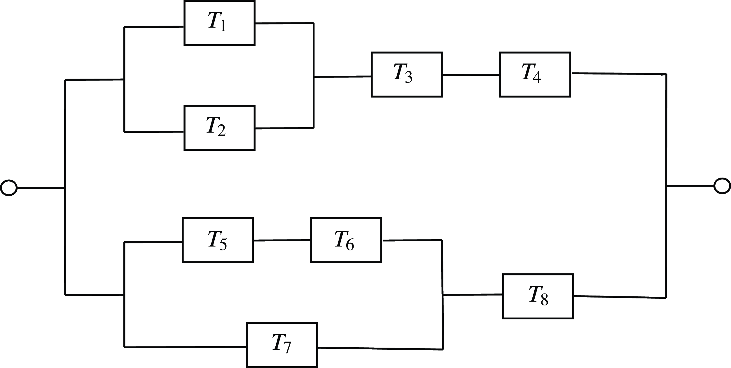
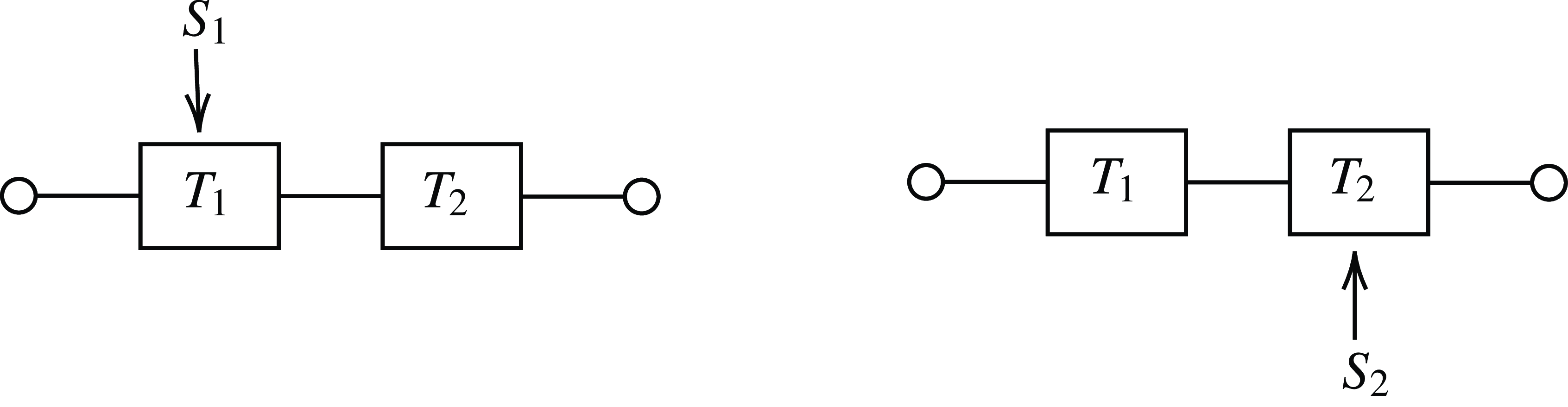
 U1
 U2
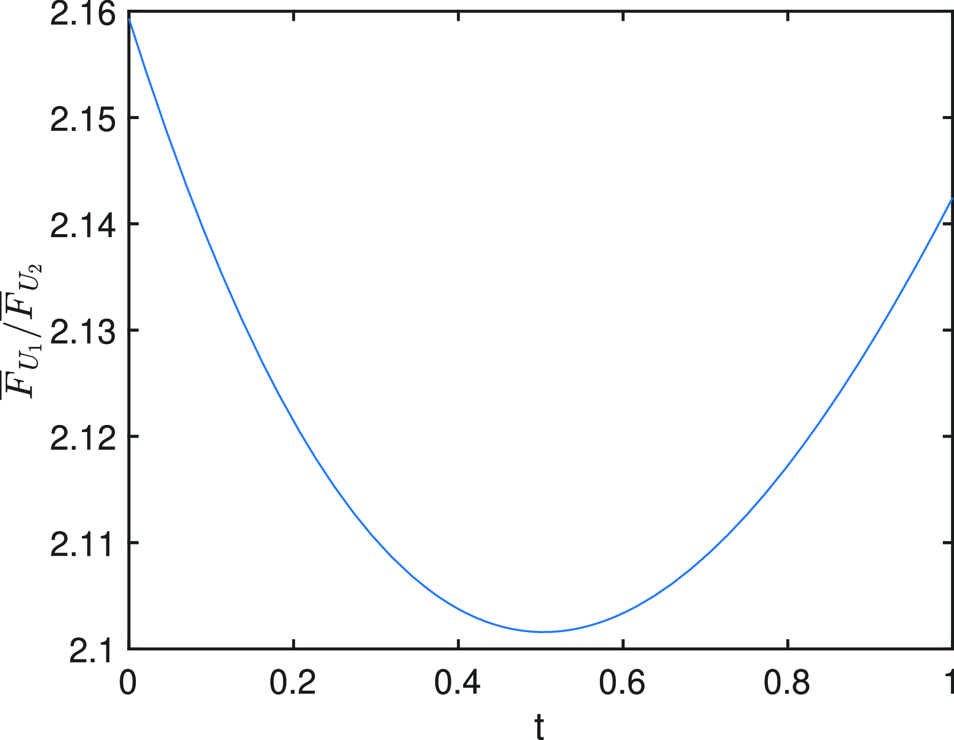
 U1
 U2
 F¯U1(t)/F¯U2(t)
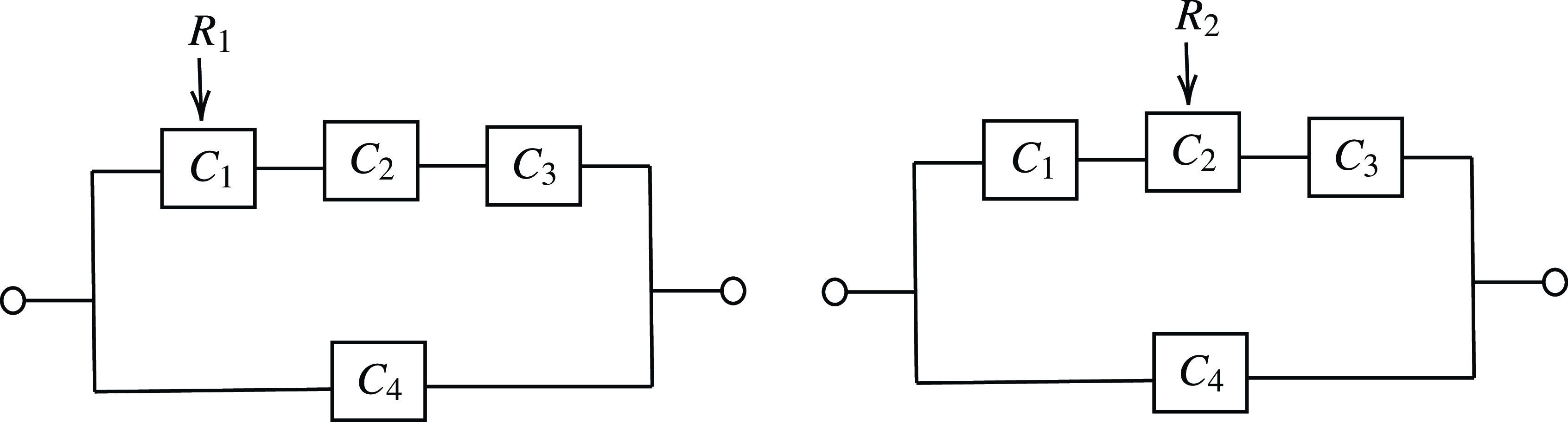
 W1
 W2

 T1
 T2
 FT1(t)andFT2(t)
 T2
 T1
 FT2(t)/FT1(t)
 T2
 T1
 fT2(t)/fT1(t)
 V1′
 V2′
 F¯V1′(t)−F¯V2′(t)
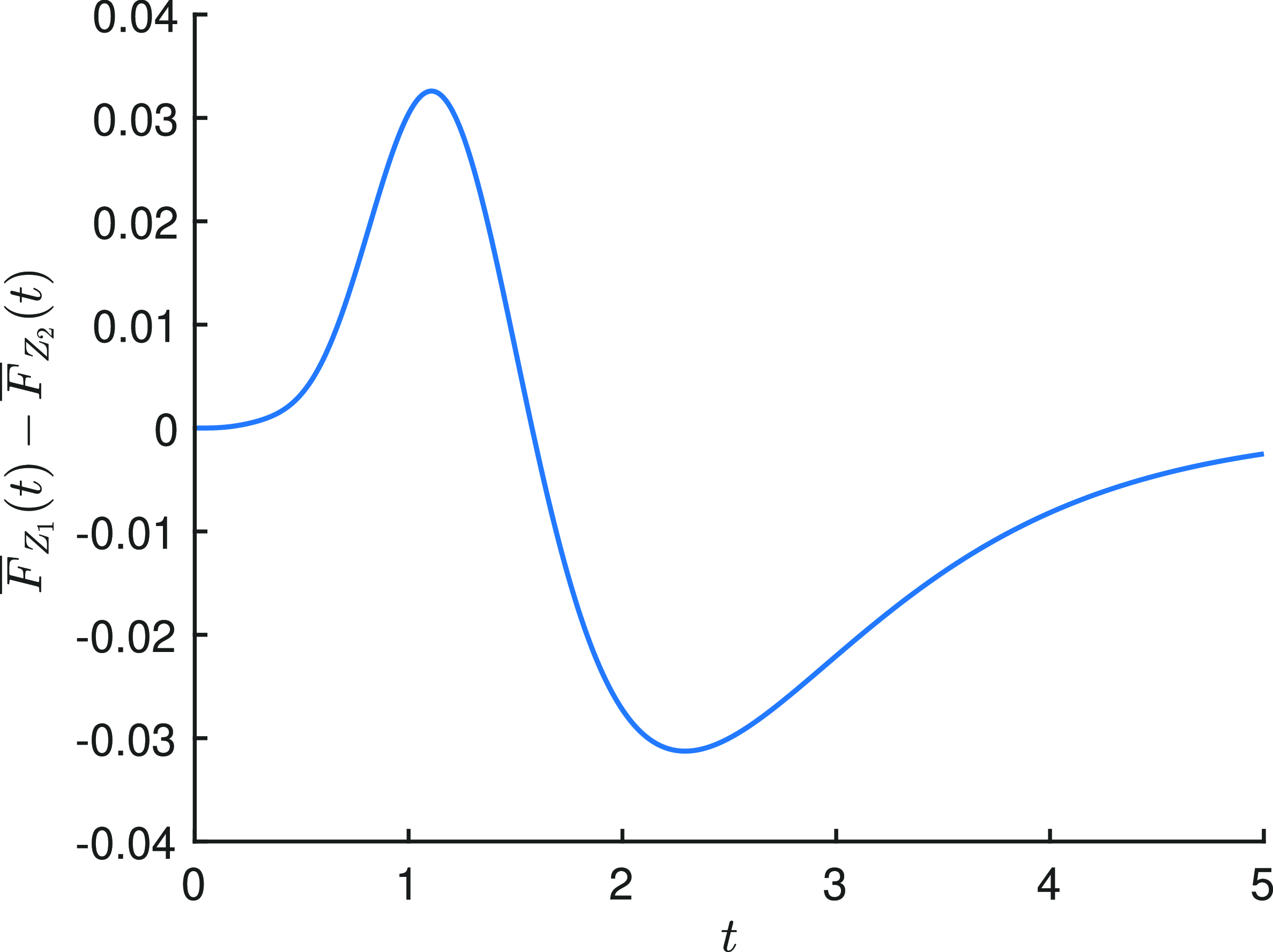
 Z1
 Z2
 F¯Z1(t)−F¯Z2(t)
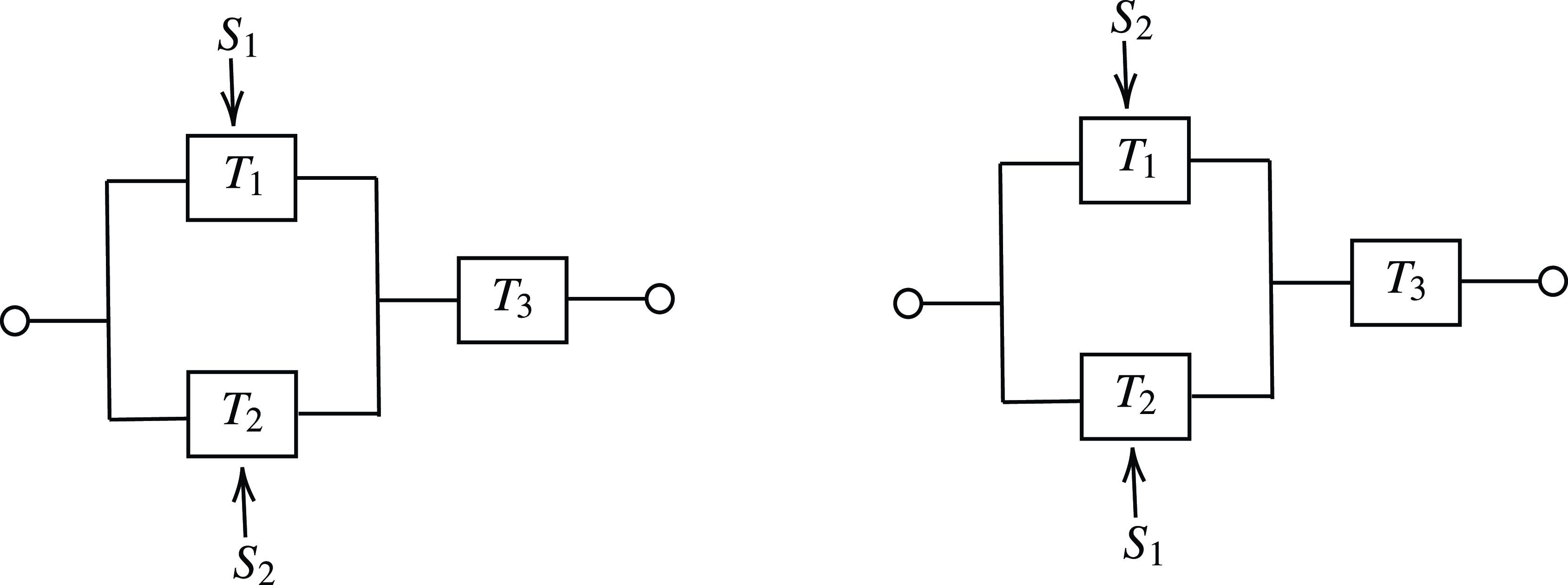
 Z1
 Z2

 Z1
 Z2
 FZ1(t)/FZ2(t)
 Z1
 Z2
 F¯Z1(t)/F¯Z2(t)
 Z1
 Z2
 F¯Z1(t)−F¯Z2(t)
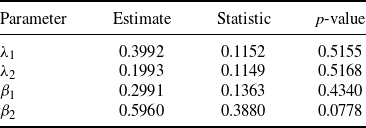
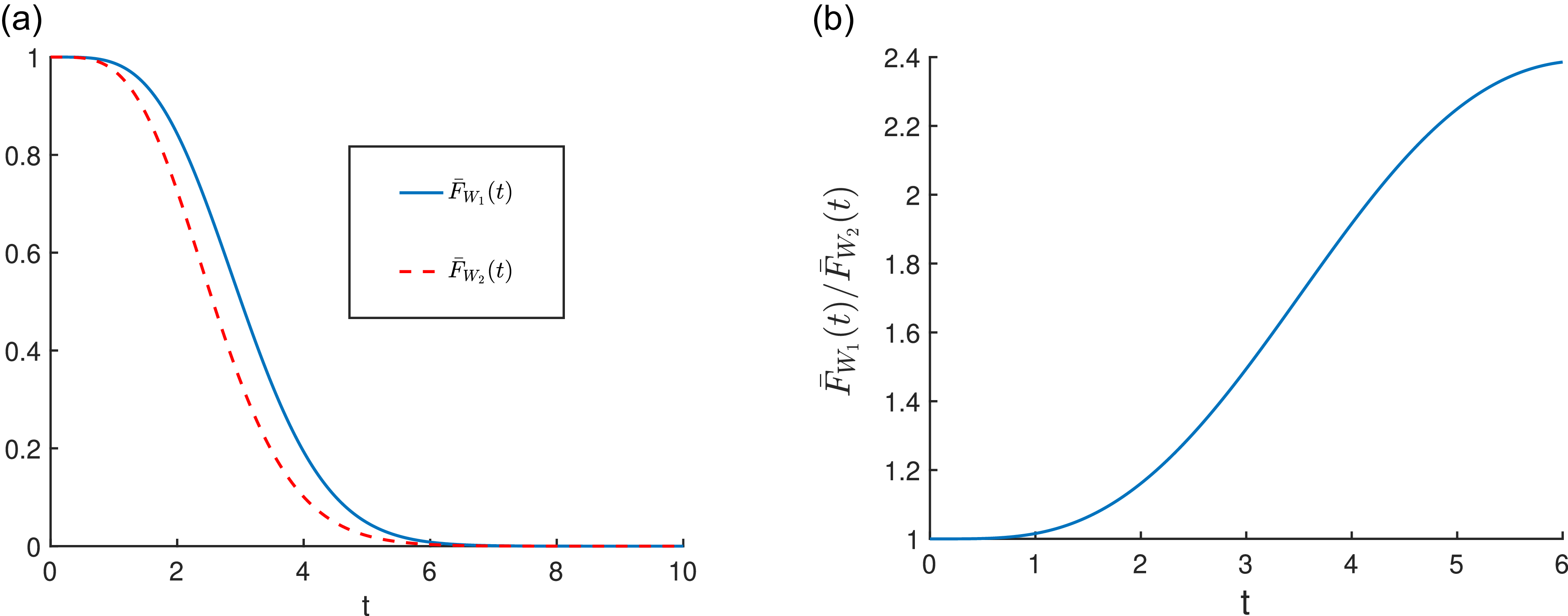
 W1
 W2
 (i.e. F¯W1(t)andF¯W2(t))
 W1
 W2
 (i.e. F¯W1(t)/F¯W2(t))
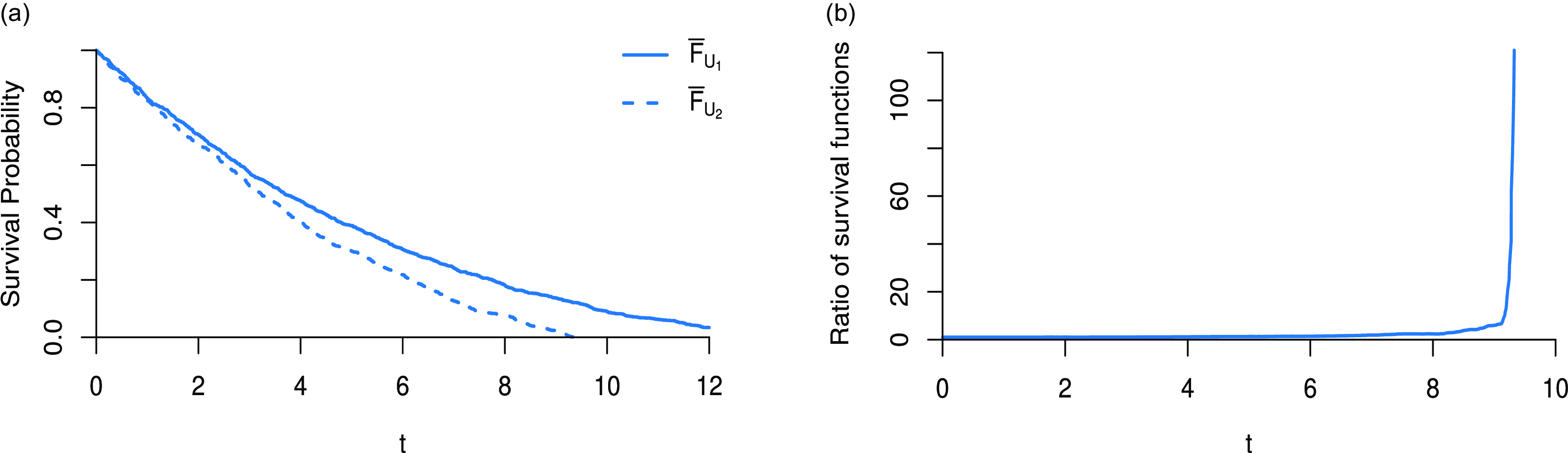
 U1
 U2
 (i.e. F¯U1(t)andF¯U2(t))
 U1
 U2
 (i.e. F¯U1(t)/F¯U2(t))
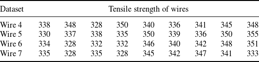
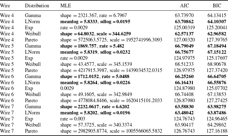
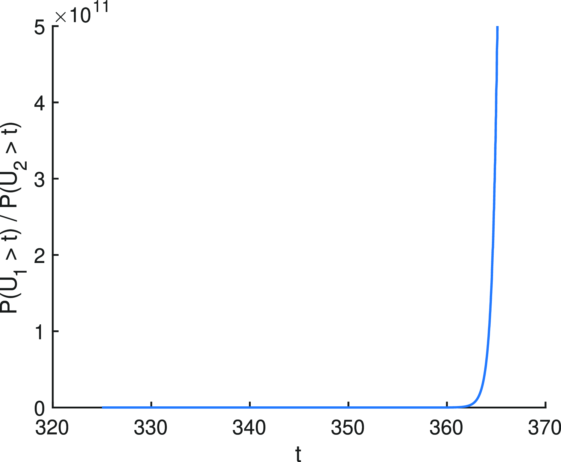
 U1
 U2
 F¯U1(t)/F¯U2(t)

 U1
 U2
 F¯U1(t)/F¯U2(t))


