1 Introduction
Let
$f:\mathbb {R}^2 \longrightarrow \mathbb {R}^2$
 be an orientation-preserving and fixed-point free homeomorphism, often referred to as a Brouwer homeomorphism. Such maps are named after Brouwer, who first studied them in the early twentieth century. In his seminal work [Reference BrouwerBro12], Brouwer proved the Brouwer translation theorem (BTT), which asserts that through every point of the plane passes a Brouwer line
$\unicode{x3bb} $
 of f, that is, a proper embedding
$\unicode{x3bb} : \mathbb R \longrightarrow \mathbb R^2$
 such that

By the Jordan curve theorem,
$\unicode{x3bb} $
 admits a left side and a right side, denoted
$L(\unicode{x3bb} )$
 and
$R(\unicode{x3bb} )$
 , corresponding to the connected components of
$\mathbb R^2\setminus \unicode{x3bb} $
 lying to the left and right of
$\unicode{x3bb} $
 .
In particular, the BTT implies that the plane can be covered by unbounded simply connected open f-invariant subsets, on which f is conjugate to a translation. This means that every point is wandering under f and, thus, the limit set of every orbit of f is empty. In other words, every orbit of f is the image of a proper embedding of
$\mathbb Z$
 into
$\mathbb R^2$
 . This fundamental description of the dynamics of Brouwer homeomorphisms became a basis for the development of Brouwer theory in the twentieth century (see [Reference GuillouGui94] for a historic account).
In the early 2000s, Le Calvez introduced a foliated version of the BTT [Reference Le CalvezLC04] (and its equivariant form in [Reference Le CalvezLC05]), thereby initiating the so-called foliated Brouwer theory, a powerful framework for studying Brouwer homeomorphisms.
Theorem. (Le Calvez [Reference Le CalvezLC04])
There exists an oriented topological foliation
${\mathcal {F}}$
 of the plane such that every leaf
$\phi \in {\mathcal {F}}$
 is a Brouwer line of f.
A foliation
${\mathcal {F}}$
 of the plane by Brouwer lines of f is called a transverse foliation of f. Although such a transverse foliation is not unique, its existence already yields a robust structure for studying the dynamics of f. Indeed, one may connect any point
$x \in \mathbb {R}^2$
 to its image
$f(x)$
 by a path
$\gamma _x : [0,1] \longrightarrow \mathbb {R}^2$
 that is positively transverse to
${\mathcal {F}}$
 , i.e.
$\gamma _x$
 intersects any leaf
$\phi \in {\mathcal {F}}$
 at most once, passing from
$R(\phi )$
 to
$L(\phi )$
 . This allows one to represent the orbit
${O} = {O}(f,x)$
 of x under f by an embedded line
$\Gamma _{O}:\mathbb R^2\longrightarrow \mathbb R^2$
 given by the concatenation

We refer to
$\Gamma _{O}$
 as a transverse trajectory of the orbit
${O}$
 , with respect to the foliation
${\mathcal {F}}$
 . Since the choice of paths
$\gamma _{f^n(x)}$
 is not unique, the orbit
${O}$
 admits uncountably many transverse trajectories
$\Gamma _{O}$
 with respect to the same foliation
${\mathcal {F}}$
 , many of which not being properly embedded. Nevertheless, all such transverse trajectories
$\Gamma _{O}$
 intersect exactly the same set of leaves of
${\mathcal {F}}$
 . Although this approach loses some qualitative dynamical information of the orbit, it has proved remarkably effective for reproducing classical results in surface dynamics and for establishing new powerful criteria for detecting chaotic behavior in surface homeomorphisms isotopic to the identity, through the celebrated forcing theory [Reference Le Calvez and TalLCT22].
There are some problems, however, that cannot be addressed using the current methods of foliated Brouwer theory. For instance, when tackling the study of Brouwer mapping classes in homotopy Brouwer theory (see [Bav17, Han99, LR17]), it is important to know whether the transverse trajectories
$\{\Gamma _{O}\}_{{O} \in {\mathcal {O}}}$
 of a finite collection
${\mathcal {O}}$
 of orbits of f can be chosen to be properly embedded and with minimal pairwise intersections.
In this work, we refine the methods of foliated Brouwer theory to address such problems, centered around future applications to the study of homotopy Brouwer theory.
1.1 Description of the results
Let us fix
$f:\mathbb R^2\longrightarrow \mathbb R^2$
 to be a Brouwer homeomorphism, and let
${\mathcal {F}}$
 be a transverse foliation of f. The set of all orbits of f is denoted by
$\mathrm {Orb}(f)$
 .
To each
${O} \in \mathrm {Orb}(f)$
 , we associate the set of leaves
$C_{O} \subset {\mathcal {F}}$
 crossed by
${O}$
 , defined as

where
$\Gamma _{O}$
 is any transverse trajectory of
${O}$
 . This set is independent of the choice of
$\Gamma _{O}$
 .
By abuse of notation, one may treat
$C_{O}$
 as a subset of
$\mathbb R^2$
 by identifying
${C_{O} = \bigcup _{\phi \in C_{O}}\phi }$
 . In §2.2, we show that
$C_{O}\subset \mathbb R^2$
 is homeomorphic to
$\mathbb{R}^2$
 and trivially foliated by
${\mathcal {F}}$
 . Moreover, the boundary
$\partial C_{O}$
 is formed by a locally finite collection of leaves of
${\mathcal {F}}$
 . At last, we define two distinguished subsets
$\partial _L C_{O}$
 and
$\partial _R C_{O}$
 of the boundary
$\partial C_{O}$
 , given by

and a total order
$\prec $
 among the leaves in
$\partial _L C_{O}$
 and similarly for
$\partial _R C_{O}$
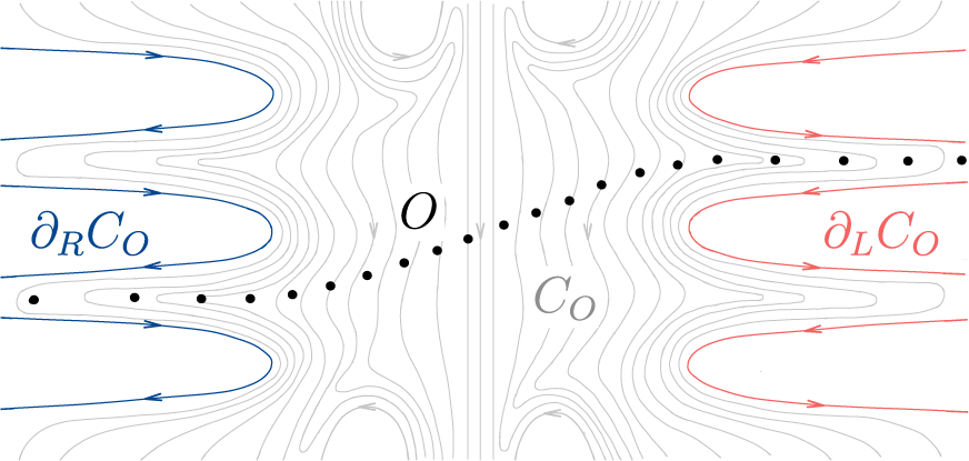
 (see Figure 1).
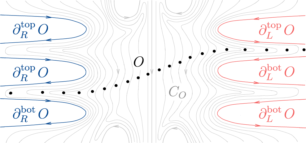
The set
$C_{O}$
 of leaves of
$\mathcal{F}$
 crossed by the orbit
${O}$
 (light gray), with its right boundary
$\partial_R C_O$
 (blue) and left boundary
$\partial_L C_O$
 (red). Note that the terms left and right are given by the orientation of the leaves in
$C_O$
 (color figures are available online).

Figure 1 Long description
A mathematical vector field diagram composed of numerous thin gray contour lines.
* On the far left, three prominent blue U-shaped curves with inward-pointing arrows represent the right boundary, labeled partial sub R C sub O.
* In the center, the gray contour lines flow vertically. A diagonal path of black dots, representing the orbit O, ascends from the lower left to the upper right, crossing through the center.
* To the right of the center, the label C sub O is placed among the gray leaves.
* On the far right, three prominent red U-shaped curves with outward-pointing arrows represent the left boundary, labeled partial sub L C sub O.
* The orientation of the leaves determines the left and right designations, with the blue boundary on the left side of the visual frame being the right boundary of the set, and the red boundary on the right side of the visual frame being the left boundary of the set.
Let
$\text {Cut}_\prec (\partial _L C_{O})$
 denote the set of all cuts of the totally ordered set
$(\partial _L C_{O},\prec )$
 , that is, the set of all pairs
$(A,B)$
 such that
$A, B \subset \partial _L C_{O}$
 are disjoint subsets of
$\partial _L C_{O}$
 satisfying:
-
• $A \cup B = \partial _L C_{O}$
 ;
-
• for any leaf $\phi \in A$
and any leaf
$\phi ' \in B$
, it holds that
$\phi \prec \phi '$
.



Similarly, let
$\text {Cut}_\prec (\partial _R C_{O})$
 denote the set of all cuts of the totally ordered set
$(\partial _R C_{O},\prec )$
 .
Definition 1.1. A proper transverse trajectory
$\Gamma _{O}$
 of an orbit
${O} \in \mathrm {Orb}(f)$
 is a transverse trajectory which is, in addition, a proper embedding of
$\mathbb R$
 into the plane.
The following result shows that such a trajectory always exists, and that it canonically determines and is determined by a pair of cuts.
Theorem A. Every orbit
${O} \in \mathrm {Orb}(f)$
 is canonically associated to two cuts

In addition, the orbit
${O}$
 admits a proper transverse trajectory
$\Gamma _{O}$
 , and it must satisfy

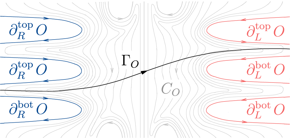
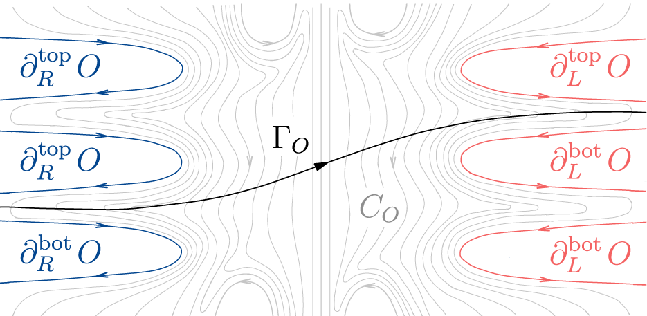
The cuts
$(\partial_L^{\mathrm{top}} O, \partial_L^{\mathrm{bot}} O)$
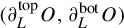 and
$(\partial_R^{\mathrm{top}} O, \partial_R{^\mathrm{bot}} O)$
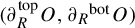 canonically associated to the orbit
$O$
 .

Figure 2 Long description
A vector field diagram featuring a central black arrowed curve labeled Gamma sub O that rises from left to right. A vertical line divides the field into two halves. In the center right, a grey label C sub O is placed among faint grey contour lines. On the left side, three blue U-shaped curves point toward the center. The top two are labeled partial sub R super top O and the bottom one is labeled partial sub R super bot O. On the right side, three red U-shaped curves point toward the center. The top one is labeled partial sub L super top O and the bottom two are labeled partial sub L super bot O. The background is filled with light grey streamlines that flow vertically and curve around these defined boundaries.
For the sake of visual intuition, we adopt the convention
$\partial^{\mathrm{top}} \prec \partial^{\mathrm{bot}}$
 (see Figure 2).
As a consequence of Theorem A, we obtain a finer description of the behavior of orbits in terms of the structure of the transverse foliation
${\mathcal {F}}$
 , given by the set
$C_{O}$
 , and the associated cuts
$(\partial _L^{\mathrm {top}} {O},\partial _L^{\mathrm {bot}} {O})$
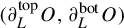 and
$( \partial _R^{\mathrm {top}} {O},\partial _R^{\mathrm {bot}} {O})$
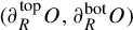 , or dually, by its proper transverse trajectories. The qualitative data are referred throughout the text as the
${\mathcal {F}}$
 -asymptotic behavior of
${O}$
 .
Being able to describe the
${\mathcal {F}}$
 -asymptotic behavior refines the framework, for instance, by allowing us to distinguish orbits of f even when they cross the same leaves of
${\mathcal {F}}$
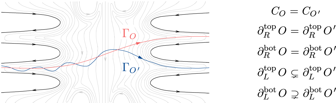
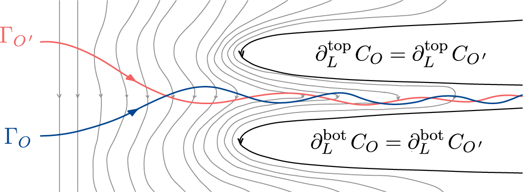
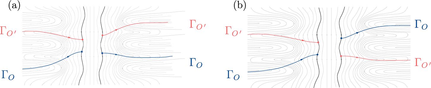
 , something not achievable before. This is illustrated in the following example (see Figure 3).
Example of orbits
$O$
 and
${O}^{\prime }$
 crossing the same leaves of
$\mathcal{F}$
 , but with distinct
$\mathcal{F}$
 -asymptotic behavior.

Figure 3 Long description
The left panel shows a vector field with light gray contour lines and several black U-shaped trajectories entering and exiting from the left and right margins. Two primary orbits cross the center. A red line labeled Gamma sub O moves from the lower left toward the upper right with a smooth curve. A blue line labeled Gamma sub O prime moves from the center left with an oscillating wave pattern, crosses the red line, and exits toward the lower right. Arrows on these lines indicate a left-to-right flow. The right panel lists five equations. 1. C sub O equals C sub O prime. 2. partial sub R super top O equals partial sub R super top O prime. 3. partial sub R super bot O equals partial sub R super bot O prime. 4. partial sub L super top O is a proper subset of partial sub L super top O prime. 5. partial sub L super bot O is a proper superset of partial sub L super bot O prime.
Definition 1.2. Two orbits
${O}, {O}^{ \prime } \in \mathrm {Orb}(f)$
 are forward
${\mathcal {F}}$
 -asymptotic, denoted
${O} \stackrel {+}{\sim } {O}^{\prime }$
 , if there exists a leaf
$\phi \in C_{O} \cap C_{{O}^{\prime }}$
 such that
$L(\phi ) \cap C_{O} = L(\phi ) \cap C_{{O}^{\prime }}$
 and, in addition,

Similarly, we define backward
${\mathcal {F}}$
 -asymptotic, denoted
${O} \stackrel {-}{\sim } {O}^{\prime }$
 , by replacing each L for R.
By comparing the different
${\mathcal {F}}$
 -asymptotic behaviors induced by the foliation
${\mathcal {F}}$
 , we obtain two relations
$\lesssim _L$
 and
$\lesssim _R$
 on the set
$\mathrm {Orb}(f)$
 , which describe how the orbits are arranged with respect to
${\mathcal {F}}$
 . For a definition of these relations, we refer to §4.1.
For each
$\phi \in {\mathcal {F}}$
 , the relations
$\lesssim_L$
 and
$\lesssim_R$
 restrict to total preorders on the subset

and are compatible with the
$\mathcal{F}$
 -asymptotic relations
$\stackrel{+}{\sim}$
 and
$\stackrel{-}{\sim}$
 , respectively (see §4.1).
Theorem B. Let
$\phi \in {\mathcal {F}}$
 and let
${\mathcal {O}}\subset \mathrm {Orb}(\phi )$
 be a finite collection of orbits crossing
$\phi $
 . Assume that
${\mathcal {F}}$
 is generic for
${\mathcal {O}}$
 , that is, no leaf in
${\mathcal {F}}$
 intersects more than one orbit in
${\mathcal {O}}$
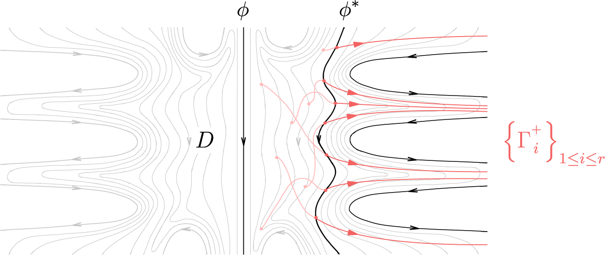
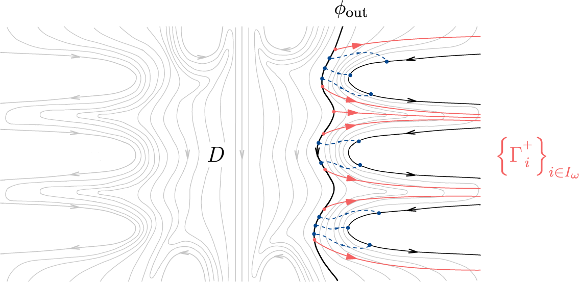
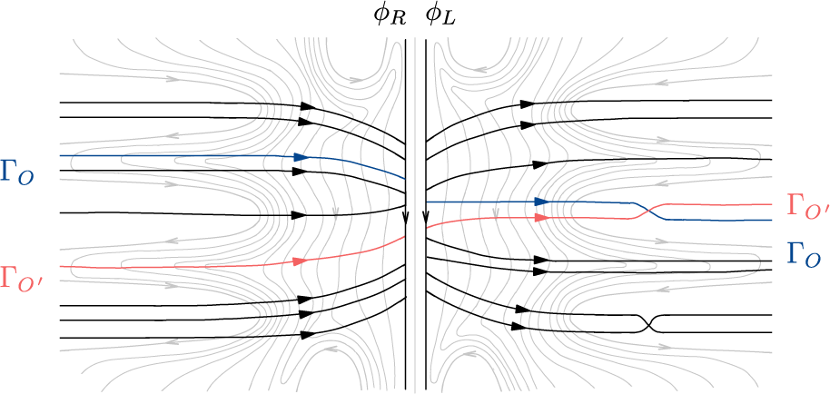
 . Then, there exists a family
$\{\Gamma _{{O}}\}_{{O} \in {\mathcal {O}}}$
 of proper transverse trajectories of
${\mathcal {O}}$
 that satisfy

Moreover, the order at which the intersection points
$p_{O} \in \Gamma _{{O}} \cap \phi $
 appear along the leaf
$\phi $
 is compatible with
$\lesssim _L$
 , i.e.,
$p_{O} < p_{{O}^{\prime }}$
 along
$\phi $
 only if
${O} \lesssim _L {O}^{\prime }$
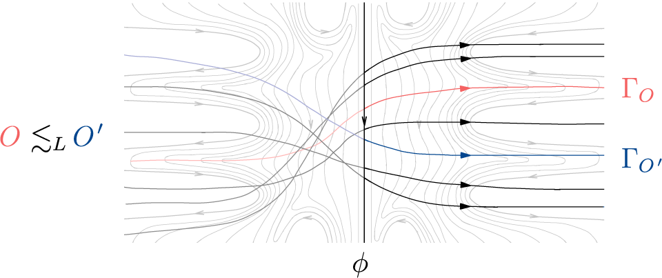
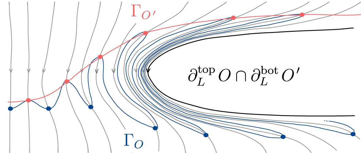
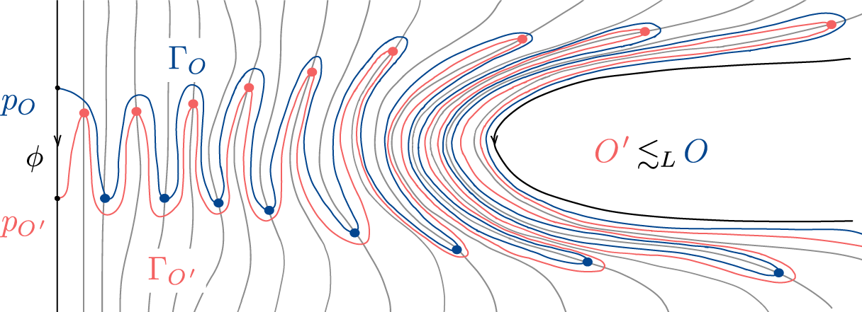
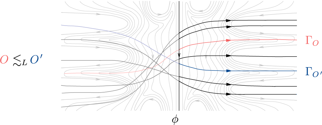
 (see Figure 4).
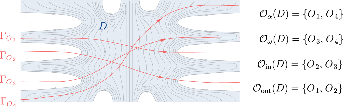
Family of proper transverse trajectories
$\{\Gamma_{O}\}_{O \in \mathcal{O}}$
 obtained in Theorem B.

Figure 4 Long description
A phase portrait featuring a dense field of light gray streamlines. A prominent vertical black line in the center is labeled with the Greek letter phi at the bottom. To the left of the field, a mathematical expression reads O is less than or approximately equal to sub L O prime.
Several bold trajectories cross the vertical phi axis from left to right.
* A red trajectory originates on the left, crosses the phi axis, and is labeled Gamma sub O on the right.
* A blue trajectory originates on the left, crosses the phi axis below the red one, and is labeled Gamma sub O prime on the right.
* Four additional bold black trajectories with arrowheads indicating rightward flow also cross the central axis.
The background streamlines form a saddle-like flow pattern, with curves diverging away from the central vertical axis toward the top and bottom edges while converging toward the horizontal midline.
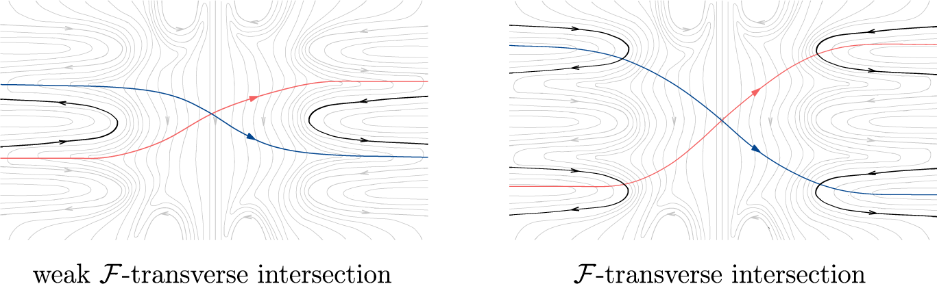
Finally, we introduce the notion of weak
${\mathcal {F}}$
 -transverse intersection between two orbits, which generalizes the notion of
${\mathcal {F}}$
 -transverse intersection defined by Le Calvez and Tal in [Reference Le Calvez and TalLCT18]. Roughly speaking, two orbits
${O}$
 and
${O}^{\prime }$
 have a weak
${\mathcal {F}}$
 -transverse intersection if they are ordered by
$\lesssim _L$
 and
$\lesssim _R$
 exclusively in opposite ways (see Figure 5).
Definition 1.3. Two orbits
${O}, {O}^{ \prime } \in {\mathrm {Orb}}(f)$
 are said to have a weak
${\mathcal {F}}$
 -transverse intersection if they satisfy
${O}\not\stackrel{+}{\sim} {O}^{\prime }$
 and
${O}\not\stackrel{-}{\sim} {O}^{\prime }$
 , and they are oppositely ordered by
$\lesssim _L$
 and
$\lesssim _R$
 , meaning that

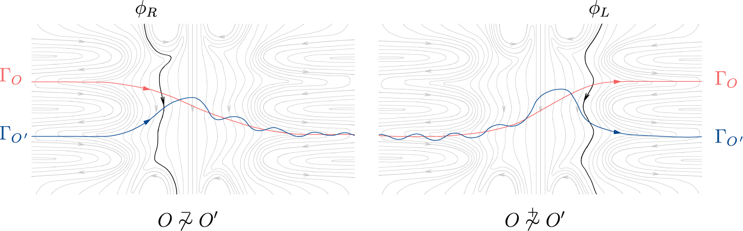
In Figure 5, we compare the classic and weak notions of
${\mathcal {F}}$
 -transverse intersection.
Comparison between the classic and weak
$\mathcal{F}$
 -transverse intersections.

Figure 5 Long description
Two side-by-side panels show streamline patterns in light gray.
Left panel labeled weak script F-transverse intersection. The background consists of horizontal streamlines that curve around central vertical regions. A blue line enters from the left, dips slightly, and exits to the right. A red line enters from the bottom-left, crosses the blue line at a shallow angle in the center, and exits to the top-right. Black U-shaped lines flank the intersection on the left and right, pointing inward.
Right panel labeled script F-transverse intersection. The background streamlines are more densely packed and exhibit sharper vertical oscillations. The blue line enters from the top-left, descends steeply through the center, and exits at the bottom-right. The red line enters from the bottom-left, ascends through the center, and exits at the top-right. The intersection angle between the red and blue lines is significantly steeper than in the left panel. Multiple black U-shaped curves are stacked vertically on both the left and right sides of the central crossing.
Before stating Theorem C, we need to introduce some terminology. Denote the open unit disk by
$\mathbb D^2 = \{(x,y) \in \mathbb R^2 \mid x^2 + y^2 < 1\}$
 . A foliation of
$\mathbb D^2$
 is said to be nicely extended to the boundary if each leaf of the foliation can be extended to a simple arc in the closed disk
$\overline {\mathbb D^2}$
 with distinct endpoints on the boundary
$\partial \mathbb D^2$
 . For any foliation
${\mathcal {F}}$
 of the plane and any homeomorphism
$\varphi :\mathbb R^2 \longrightarrow \mathbb D^2$
 , we denote by
$\varphi ({\mathcal {F}})$
 the foliation of
$\mathbb D^2$
 formed by the images of the leaves of
${\mathcal {F}}$
 under
$\varphi $
 . Finally, a diagram is a finite collection of oriented line segments in
$\mathbb D^2$
 with pairwise distinct endpoints on the boundary
$\partial \mathbb D^2$
 .
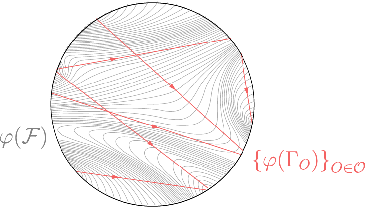
Theorem C. Let
${\mathcal {O}}\subset \mathrm {Orb}(f)$
 be a finite collection of orbits and assume
${\mathcal {F}}$
 is generic for
${\mathcal {O}}$
 . Then, there exists a family
$\{\Gamma _{O}\}_{{O} \in {\mathcal {O}}}$
 of proper transverse trajectories for
${\mathcal {O}}$
 and a homeomorphism
$\varphi :\mathbb R^2 \longrightarrow \mathbb D^2$
 that satisfy (see Figure 6) the following properties:
-
(i) the foliation $\varphi ({\mathcal {F}})$
is nicely extended to the boundary; -
(ii) the family $\{\varphi (\Gamma _{O})\}_{{O} \in {\mathcal {O}}}$
is a diagram in
$\mathbb D^2$
; -
(iii) two distinct segments $\varphi (\Gamma _{O})$
and
$\varphi (\Gamma _{{O}^{\prime }})$
intersect if, and only if, the orbits
${O}$
and
${O}^{\prime }$
have a weak
${\mathcal {F}}$
-transverse intersection.


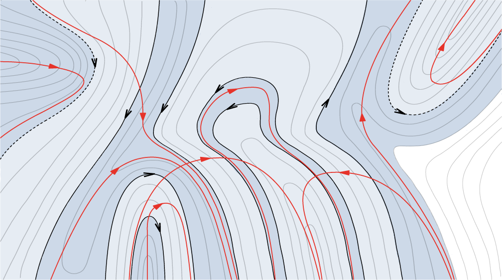
Diagram of proper transverse trajectories described by Theorem C.

Figure 6 Long description
A circular diagram containing a dense background of fine grey lines representing a foliation labeled phi (F) on the left. These grey lines form various curved patterns, including concentric loops in the lower-left quadrant and asymptotic flows toward the boundary. Overlaid on this field are several thick red lines with arrowheads indicating direction, labeled as the set of phi (Gamma sub O) for O in O on the bottom-right. These red trajectories cross the grey lines transversely. One red line enters from the top-left and moves toward the center-right. Another enters from the mid-left, reflecting off the boundary to move toward the bottom-right. A third red line is visible near the bottom, moving from left to right across the curved grey structures.
2 Preliminaries
2.1 Planar topology
Let
$\mathbb R^2$
 be the Euclidean plane, equipped with the topology induced by the Euclidean metric d. An open ball of radius
$r>0$
 centered at
$x\in \mathbb R^2$
 is denoted by
$B(x,r)$
 .
A path
$\gamma : I\longrightarrow \mathbb R^2$
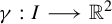 is a continuous map defined on an interval
$I\subset \mathbb R$
 . A path
$\gamma $
 is said to be a reparameterization of another path
$\gamma ':I'\longrightarrow \mathbb R^2$
 if there exists a strictly increasing map
$\varphi :\mathbb R\longrightarrow \mathbb R$
 that satisfies
$\varphi (I) = I'$
 and
$\gamma = \gamma ' \circ \varphi \vert _I$
 . A loop
$\gamma :\mathbb {S}^1\longrightarrow \mathbb R^2$
 is a continuous map defined on the unit circle
$\mathbb {S}^1$
 . A path or a loop is said to be simple if it is injective. By abuse of notation, if there is no ambiguity, we may consider paths and loops as subset of the plane by identifying them with their images.
A topological line is a path
$\ell : \mathbb R \longrightarrow \mathbb R^2$
 that is injective and proper. Observe that any topological line admits a natural orientation induced by the positive orientation on
$\mathbb R$
 . Similarly, we define a half-line as a path
$\ell ^+: [0,\infty )\longrightarrow \mathbb R^2$
 that is injective and proper. Often enough, it is convenient to consider half-lines defined on
$(-\infty ,0]$
 as well.
In the sphere compactification of the plane
$\mathbb {S}^2 = \mathbb R^2 \sqcup \{\infty \}$
 , every topological line
$\ell $
 can be extended to a simple loop on
$\mathbb S^2$
 by adding the point at infinity. According to the Jordan curve theorem [Reference JordanJor87], the complement of any simple loop on the sphere has exactly two connected components. By the Schoenflies theorem (see [Reference CairnsCai51] for an elementary proof), each of these connected components is homeomorphic to
$\mathbb R^2$
 . In our context, this means that every topological line
$\ell $
 separates the plane into two sets, each of which is homeomorphic to the plane. These sets are called the left and right sides of
$\ell $
 , denoted
$ L(\ell ) $
 and
$ R(\ell ) $
 , according to the orientation of
$\ell $
 .
Now, we present a fundamental generalization of the Schoenflies theorem, which provides a criterion for extending homeomorphisms defined on subsets of the sphere to the entire sphere. This theorem is particularly useful in the context of low-dimensional topology because it allows us to handle ‘nice’ subsets of
$\mathbb{S}^2$
 with more flexibility.
Here, by arc, we mean a simple path
$\gamma : [0,1] \longrightarrow \mathbb S^2$
 . A Y-set is a subset of
$\mathbb S^2$
 , which is the union of three arcs intersecting at a single point that is an endpoint of each arc. Note that the orientation of
$\mathbb S^2$
 induces a cyclic order on the arcs constituting a Y-set in a neighborhood of the intersection point.
Theorem. (Homma–Schoenflies) [Reference HommaHom53]
Let
$X\subset \mathbb S^2$
 be a compact, connected, and locally connected set. Then, an injective and continuous map
$h:X\longrightarrow \mathbb S^2$
 can be extended to an orientation-preserving homeomorphism of
$\mathbb S^2$
 if, and only if, the map h preserves the cyclic order of any Y-set contained in X.
Applying the Homma–Schoenflies theorem is not necessarily straightforward, as it requires checking the preservation of the cyclic order of Y-sets. However, there are many classic examples of applications of this theorem (see [Reference Le RouxLR06, Appendix]). Along this preliminary section, we will guide the reader through the process of applying the Homma–Schoenflies theorem as we introduce the new concepts and tools.
A family
$\{A_i\}_{i \in I}$
 of subsets of
$\mathbb R^2$
 is called locally finite if, for every compact set
${K\subset \mathbb R^2}$
 , we have that
$\{i \in I \mid A_i \cap K \neq \varnothing \}$
 is a finite set.
Lemma 2.1. Let
$\{X_i\}_{i \in I}$
 be a family of locally finite and pairwise disjoint closed subsets of the plane. Then, there exists a locally finite family
$\{U_i\}_{i\in I}$
 of pairwise disjoint open subsets that satisfy
$X_i \subset U_i$
 , for every
$i \in I$
 .
Proof. For each
$i \in I$
 , consider the set
$Y_i:=\bigcup _{j \in I} X_j \setminus X_i$
 . First, we show that
$Y_i$
 is closed. For a given
$i \in I$
 , let
$(x_n)_{n\in \mathbb N}$
 be a sequence of points in
$Y_i$
 that converges to a point
$x\in \mathbb R^2$
 . Observe that, since the family
$\{X_j\}_{j \in I}$
 is locally finite, the set
$\{j \in I \mid d(x, X_j) < r\}$
 is finite for any
$r>0$
 . Consequently, there exists an index
$j_0 \in I\setminus \{i\}$
 and a subsequence
$(x_{n_k})_{k\in \mathbb N}$
 that satisfies
$x_{n_k} \in X_{j_0}$
 for every
$k\in \mathbb N$
 . Since
$X_{j_0}$
 is a closed set, we have that
$x \in X_{j_0}$
 . Since
$X_{j_0}$
 is disjoint from
$X_i$
 , we have that
$x \not \in X_i$
 . This allows us to conclude that
$x \in Y_i$
 , which proves that the set
$Y_i$
 is closed.
We can now define, for each
$i \in I$
 , the set
Since
$X_i$
 and
$Y_i$
 are disjoint sets, we observe that

This proves that
$X_i \subset U_i$
 for every
$i \in I$
 . Next, we remark that

This implies that
$U_i$
 is disjoint from
$U_j$
 for every
$j \in I\setminus \{i\}$
 . Finally, note that the function

is continuous. Thus, by writing
$U_i = g_i^{-1}((-\infty ,0))$
 , we conclude that
$U_i$
 is an open set.
To conclude the proof, we need to show that the family
$\{U_i\}_{i \in I}$
 is locally finite. For that, we consider for each
$i \in I$
 , the closed ball

Since the family
$\{X_i\}_{i \in I}$
 is locally finite, the family of closed balls
$\{B(X_i,1)\}_{i \in I}$
 is also locally finite. From the definition of the set
$U_i$
 , we can observe that

Therefore, we conclude that the family of open sets
$\{U_i\}_{i \in I}$
 also is locally finite.
Here, we provide a first application of the Homma–Schoenflies theorem.
Let
$\{\ell _{n}\}_{n\in \mathbb Z}$
 be a locally finite family of pairwise disjoint topological lines such that

In this context, the union of the lines in the family
$\{\ell _n\}_{n \in \mathbb Z}$
 and the point at infinity forms a compact, connected, and locally connected subset of
$\mathbb S^2$
 . It is worth noting that this would not be the case if the family
$\{\ell _n\}_{n \in \mathbb Z}$
 was not locally finite. Using the Homma–Schoenflies theorem, we can obtain an orientation-preserving homeomorphism on the plane that maps each line
$\ell _n$
 to the vertical line
$\{n\}\times \mathbb R$
 oriented downwards.
For more applications, we refer the reader to [Reference Le RouxLR17, Appendix B].
2.2 Topological planar foliations
A topological planar foliation
$\mathcal {F}$
 is a partition of the plane into disjoint topological lines, called leaves, that admits a local parallel structure. In other words, for any point
$x \in \mathbb {R}^2$
 , there exists a closed neighborhood
$U\subset \mathbb R^2 $
 of x and a homeomorphism
$\varphi : U \to [0,1] \times [0,1]$
 such that, for every leaf
$\phi \in {\mathcal {F}}$
 , each connected component of the set
$\phi \cap U$
 is of the form
$\varphi^{-1}(\{t\} \times [0,1]).$

In the particular case of foliations of
$\mathbb R^2$
 , the condition above can be exchanged for the condition that the entire set
$\phi \cap U$
 is of the form
$\varphi ^{-1}(\{t\} \times [0,1])$
 for some
$t \in [0,1] $
 .
A cross-section of
${\mathcal {F}}$
 over a leaf
$\phi \in {\mathcal {F}}$
 is a compact arc
$\sigma \subset \mathbb {R}^2$
 that intersects
$\phi $
 and is transverse to
${\mathcal {F}}$
 , meaning that the arc
$\sigma $
 intersects each leaf of
${\mathcal {F}}$
 at most once.
Let
$\phi \in {\mathcal {F}}$
 be a leaf and let
$\{\sigma _k\}_{k \in \mathbb Z^*}$
 be a locally-finite collection of pairwise disjoint compact cross-sections of
${\mathcal {F}}$
 over the leaf
$\phi $
 . Assume that, for every
$k>0$
 , it holds that:
-
• the cross-sections $\sigma _{-k}$
and
$\sigma _{k}$
intersect the same leaves in
${\mathcal {F}}$
; -
• the sub-arc $u_k\subset \phi $
joining
$\sigma _{-k}$
and
$\sigma _{k}$
satisfies
$u_k \subset u_{k+1}$
; -
• the only leaf of ${\mathcal {F}}$
intersecting all cross-sections in
$\{\sigma _k\}_{k \in \mathbb N^*}$
is the leaf
$\phi $
; -
• every leaf of ${\mathcal {F}}$
that intersects
$\sigma _{k+1}$
also intersects
$\sigma _k$
.


The closed set
$V\subset \mathbb R^2$
 , obtained as the union of all compact sub-arcs of leaves in
${\mathcal {F}}$
 joining the cross-sections
$\sigma _{-k}$
 and
$\sigma _{k}$
 , for some
$k>0$
 , is a trivial neighborhood of the leaf
$\phi $
 . Observe that, for any open neighborhood
$U\subset \mathbb R^2$
 of
$\phi $
 , we can consider sufficiently small cross-sections
$\{\sigma _k\}_{k \in \mathbb Z^*}$
 so that the neighborhood V is contained in U.
It is worth noting that trivial neighborhoods of leaves can be taken to be arbitrarily small. More precisely, for any leaf
$\phi \in {\mathcal {F}}$
 and any open neighborhood
$U\subset \mathbb R^2$
 of
$\phi $
 , there exists a trivial neighborhood V of
$\phi $
 such that
$V\subset U$
 . Such a trivial neighborhood V can be obtained by taking the cross-sections in the collection
$\{\sigma _k\}_{k \in \mathbb Z^*}$
 to be sufficiently small.
By the Homma–Schoenflies theorem, for any trivial neighborhood V of a leaf
$\phi \in {\mathcal {F}}$
 , we can find a homeomorphism
$\varphi : \mathbb R^2\longrightarrow \mathbb R^2$
 that satisfies the following properties:
-
• the leaf $\phi $
is mapped by
$\varphi $
into the vertical line
$\{0\}\times \mathbb R$
; -
• the set V is mapped by $\varphi $
into the set
$\bigcup _{n \in \mathbb N^*} [-{1}/{n}, {1}/{n}]\times [ -n,n]$
; -
• for each leaf $\phi ' \in {\mathcal {F}}$
, the set
$\varphi (\phi '\cap V)$
is a vertical line
$\{t\}\times \mathbb R$
for some
$t\in \mathbb R$
.





As a direct application of Lemma 2.1, we have the following lemma, which will be of main importance in the developments of §3.
Lemma 2.2. Let
$\{\phi _i\}_{i \in I}$
 be a locally finite family of pairwise disjoint leaves of
${\mathcal {F}}$
 . Then, for any closed set
$X \subset \mathbb R^2$
 that is disjoint from all leaves in
$\{\phi _i\}_{i \in I}$
 , there exists a locally finite family of pairwise disjoint closed sets
$\{V_i\}_{i \in I}$
 such that, for each
$i \in I$
 , the set
$ V_i $
 is a trivial neighborhood of the leaf
$ \phi _i $
 that is disjoint from X.
Proof. Observe that
$\{\phi _i\}_{i \in I} \cup \{X\}$
 forms a locally finite family of pairwise disjoint closed subsets of
$\mathbb R^2$
 . By applying Lemma 2.1, we can find a locally finite family of pairwise disjoint open sets
$\{U_i\}_{i \in I}$
 such that, for each
$i \in I$
 , the set
$U_i$
 is a neighborhood of the leaf
$\phi _i$
 and is disjoint from X. Since trivial neighborhoods of leaves can be taken to be arbitrarily small, for each
$i \in I$
 , we can consider a trivial neighborhood
$V_i$
 of the leaf
$\phi _i$
 such that
$V_i \subset U_i$
 . Since
$\{U_i\}_{i \in I}$
 is locally finite, so is the family
$\{V_i\}_{i \in I}$
 .
We can endow any foliation
${\mathcal {F}}$
 with the quotient topology, which corresponds to the finest topology on
${\mathcal {F}}$
 for which the quotient map
$\pi _{_{\mathcal {F}}}:\mathbb R^2\longrightarrow {\mathcal {F}}$
 that sends each point to the leaf passing through it is continuous. In this topology, the open sets of the foliation
${\mathcal {F}}$
 are those whose preimages under
$\pi _{_{\mathcal {F}}}$
 are open in
$\mathbb R^2$
 . Throughout this text, we will always consider the quotient topology on foliations, unless otherwise stated.
A subset
$A\subset \mathbb R^2$
 is called saturated (with respect to
${\mathcal {F}}$
 ) if it contains all leaves of
${\mathcal {F}}$
 that intersect it. The restriction of a foliation
${\mathcal {F}}$
 to a saturated subset
$A\subset \mathbb R^2$
 is denoted by
${\mathcal {F}}\vert _A$
 . Note that, in the case of saturated sets, we have
${\mathcal {F}}\vert _A = \pi _{_{\mathcal {F}}}(A)$
 . By a slight abuse of notation, we often treat saturated sets
$A\subset \mathbb R^2$
 as subsets of the foliation
${\mathcal {F}}$
 by identifying
$A = {\mathcal {F}}\vert _A$
 . This is the abuse that allows us to denote saturated sets as subsets
$A\subset {\mathcal {F}}$
 or to refer to leaves as elements
$\phi \in A$
 . This convention introduces no topological ambiguity when referring to an open saturated set or to its boundary. Indeed, from the definition of the quotient topology, a saturated set
$A\subset \mathbb R^2$
 is open if, and only if, the restriction
${\mathcal {F}}\vert _A$
 is an open subset of
${\mathcal {F}}$
 . Additionally, the boundary
$\partial A$
 of a saturated set A may be understood equivalently as the boundary of A inside
$\mathbb {R}^2$
 or as the boundary of
${\mathcal {F}}|_A$
 inside
${\mathcal {F}}$
 , with no risk of confusion.
This next lemma states that the connectedness is also preserved through this notation.
Lemma 2.3. A saturated set
$A\subset \mathbb R^2$
 is connected if, and only if,
$ {\mathcal {F}}\vert _A$
 is connected.
Proof. (
$\!\implies\!$
 ) Let
$A\subset \mathbb R^2$
 be a connected saturated set. Since
$\pi _{_{\mathcal {F}}}$
 is continuous, the image
$\pi _{_{\mathcal {F}}}(A)$
 is connected. This proves the implication.
(
$\!\impliedby\! $
 ) Let us assume that
$A\subset \mathbb R^2$
 is a saturated set such that
${\mathcal {F}}\vert _A$
 is connected. Suppose by contradiction that A is not connected. Therefore, there exists two non-empty open subsets
$U,V \subset \mathbb R^2$
 such that
$A\subset U \cup V$
 and such that
$U \cap A$
 is disjoint from
$V\cap A$
 . Since each leaf
$\phi \in A$
 is connected, then either
$\phi \cap U$
 or
$\phi \cap V$
 is empty. Since A is saturated and covered by the union
$U\cup V$
 , we have that each leaf
$\phi \in A$
 is contained in either U or V. In other words,
$U \cap A$
 and
$V \cap A$
 are disjoint saturated sets that cover A. Since
$\pi _{_{\mathcal {F}}}$
 is a quotient map,
${\mathcal {F}}\vert _{U\cup A}=\pi _{_{\mathcal {F}}}(U \cap A)$
 and
${\mathcal {F}}\vert _{V\cup A}=\pi _{_{\mathcal {F}}}(V \cap A)$
 are open subsets of
${\mathcal {F}}\vert _A$
 that are disjoint and cover
${\mathcal {F}}\vert _A$
 . This contradicts the assumption that
${\mathcal {F}}\vert _A$
 is connected.
Equipped with the quotient topology, the foliation
${\mathcal {F}}$
 becomes a simply connected and non-Hausdorff one-dimensional manifold, often called the leaf space of
${\mathcal {F}}$
 . As a matter of fact, the classical result due to Haefliger and Reeb [Reference Haefliger and ReebHR57] proves that every simply connected, non-Hausdorff 1-manifold can be realized as the leaf space of a planar foliation. Note that, any simply connected (non-Hausdorff) manifold is orientable. In the one-dimensional context, this corresponds to the existence of an atlas of charts mapping the local orientation at each point of the manifold to the positive orientation of
$\mathbb R$
 . By choosing an orientation, we fix a local notion of left and right sides around each point. Since, by removing a point, we separate any simply connected non-Hausdorff 1-manifold into two connected components, this local notion of left and right sides is extended globally to each connected component.
In the context of the leaf space, this means that for each leaf
$\phi \in {\mathcal {F}}$
 , the set
${\mathcal {F}}\setminus \{\phi \}$
 has exactly two connected components, one labeled as the left side
$L(\phi )$
 and the other as the right side
$R(\phi )$
 . Each leaf of
$\mathcal {F}$
 thereby inherits an orientation and this assignment is locally coherent, since it is determined by the local orientation at each point of the leaf space. In terms of local trivializing maps of the foliation
${\mathcal {F}}$
 , this means that one can choose each trivializing map
$\varphi : U \to [0,1] \times [0,1]$
 so that the orientation of every leaf
$\phi \in {\mathcal {F}}$
 is mapped to the positive direction of the second coordinate on the set
$\varphi (U \cap \phi ) = \{t\} \times [0,1]$
 . This is the classical definition of an oriented foliation.
Once the foliation
${\mathcal {F}}$
 is equipped with an orientation, it inherits a naturally defined partial order, where
$\phi \leq \phi '$
 if and only if
$L(\phi ') \subset L(\phi )$
 . Note that pairs of leaves
$\phi ,\phi '\in {\mathcal {F}}$
 which are not Hausdorff-separable must satisfy either
$R(\phi ) \cap R(\phi ') = \varnothing $
 or
$L(\phi ) \cap L(\phi ') = \varnothing $
 and, consequently, they cannot be comparable under this partial order relation. Recall that, an interval of the foliation
${\mathcal {F}}$
 with respect to this partial order consists in a subset of
${\mathcal {F}}$
 that contains all leaves between any two of its leaves. Observe that leaf intervals are not necessarily homeomorphic to an interval of the real line
$\mathbb R$
 , as the leaf space of
${\mathcal {F}}$
 is not necessarily Hausdorff.
A saturated set
$A\subset \mathbb R^2$
 is said to be non-separating if for every leaf
$\phi \in A$
 , one of the connected components of
$\mathbb R^2\setminus \phi $
 contains all leaves in
$A\setminus \{\phi \}$
 .
Lemma 2.4. Let
$A\subset \mathbb R^2$
 be an open, connected saturated set. Then, the following hold:
-
(i) the restriction ${\mathcal {F}}\vert _A$
is an interval of the foliation
${\mathcal {F}}$
; -
(ii) the boundary $\partial A$
is a locally finite and non-separating collection of leaves in
${\mathcal {F}}$
; -
(iii) the set $A\subset \mathbb R^2$
is homeomorphic to a plane.


Proof.
Proof of item (i). Suppose by contradiction that there exist
$\phi ,\phi ' \in {\mathcal {F}}\vert _A$
 such that
$\phi < \phi '$
 , and
$\phi " \in {\mathcal {F}}\setminus {\mathcal {F}}\vert _A$
 such that
$\phi < \phi " < \phi '$
 . In this case, the sets
$L(\phi ")$
 and
$R(\phi ")$
 are disjoint open sets whose union covers A, and such that
$L(\phi ") \cap A$
 and
$R(\phi ") \cap A$
 are both non-empty. This contradicts the assumption that A is connected.
Proof of item (ii). Since
$A\subset \mathbb R^2$
 is open and connected, for any leaf
$\phi \in \partial A$
 , the set A must be contained in one of the two connected components of
$\mathbb R^2\setminus \phi $
 . Therefore, each of the remaining leaves in
$\partial A\setminus \{\phi \}$
 is contained in the same connected component of
$\mathbb R^2\setminus \phi $
 that contains A. This implies that the set
$\partial A$
 is non-separating.
Next, observe that any open set
$U\subset \mathbb R^2$
 that locally trivializes the foliation
${\mathcal {F}}$
 can at most intersect two leaves in
$\partial A$
 . This is because, for any three leaves of
${\mathcal {F}}$
 intersecting U, we get that one of them must separate the other two. Let
$K\subset \mathbb R^2$
 be a compact set and let
$\{U_i\}_{0<i<k}$
 be a finite cover of K by open sets that locally trivialize
${\mathcal {F}}$
 . Since each set in the cover
$\{U_i\}_{0<i<k}$
 intersects at most two leaves in
$\partial A$
 , the set K intersects at most finitely many leaves in
$\partial A$
 . This implies that the collection of leaves in
$\partial A$
 is locally finite.
Proof of item (iii). Knowing that the boundary
$\partial A$
 is non-separating, we can write A as the complement of the set
$\bigcup _{\phi \in \partial A} K(\phi )$
 , where
$K(\phi )$
 is defined as the closure of the connected component of
$\mathbb R^2\setminus \phi $
 that does not contain A. Observe that, by adding the point at infinity, the set
$\bigcup _{\phi \in \partial A} K(\phi )\cup \{\infty \}$
 becomes a compact and connected subset of
$\mathbb S^2$
 . Since A is the complement of a compact and connected subset of
$\mathbb S^2$
 , we conclude that it is simply connected. According to the Riemann mapping theorem, being a simply connected open subset of
$\mathbb R^2$
 , the set A must be homeomorphic to the plane. This completes the proof.
A saturated set
$A\subset \mathbb R^2$
 is said to be trivially foliated if the restriction
${\mathcal {F}}\vert _A$
 is totally ordered by the natural order on the foliation
${\mathcal {F}}$
 .
Definition 2.5. A leaf domain is a saturated set that is open, connected, and trivially foliated.
Following Lemmas 2.3 and 2.4, we observe that non-empty leaf domains of
${\mathcal {F}}$
 correspond exactly to the subsets of
${\mathcal {F}}$
 that are homeomorphic to
$\mathbb R$
 . Moreover, the boundary of a leaf domain is formed by a locally finite and non-separating collection of leaves in
${\mathcal {F}}$
 .
Lemma 2.6. A finite intersection of leaf domains also is a leaf domain.
Proof. The lemma holds because, in a simply connected non-Hausdorff 1-manifold, the intersection of two subsets homeomorphic to
$\mathbb R$
 is either empty or homeomorphic to
$\mathbb R$
 .
The boundary of a leaf domain
$A\subset {\mathcal {F}}$
 admits two important subsets, defined as

These sets are disjoint by definition and their union may not cover the entire boundary
$\partial A$
 . The set A lies on the left side of each leaf in
$\partial _R A$
 and on the right side of every leaf in
$\partial _L A$
 .
The sets
$\partial _R A$
 and
$\partial _L A$
 are each totally ordered by a relation
$\prec $
 , defined as follows.
-
• Fix a leaf of reference $\phi _* \in A$
. For any two leaves
$\phi , \phi ' \in \partial _L A$
(respectively
$\partial _R A$
), we define
$\phi \prec \phi '$
if and only if there exist two disjoint paths
$\gamma ,\gamma ':[0,1]\longrightarrow \mathbb R^2$
with endpoints
$\gamma (1) \in \phi $
,
$\gamma '(1) \in \phi '$
, and
$\gamma (0), \gamma '(0) \in \phi _*$
, ordered
$\gamma (0)< \gamma '(0) $
along the leaf
$\phi _*$
.








We remark that
$\prec $
 is well defined and independent of the choice of reference leaf
$\phi _*\in A$
 . Later, in §3.3, we provide a more formal alternative definition of this order relation.
A path
$\gamma :I\longrightarrow \mathbb R^2$
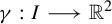 defined on an interval
$I \subset \mathbb R$
 is said to be positively transverse to an oriented foliation
${\mathcal {F}}$
 if the map
$\pi _{_{\mathcal {F}}}\circ \gamma :I\longrightarrow {\mathcal {F}}$
 is strictly increasing with respect to the natural order on
${\mathcal {F}}$
 . In other words, a positively transverse path intersects each leaf of
${\mathcal {F}}$
 at most once and it does so crossing each leaf from right to left.
Each positively transverse path
$\gamma $
 defines a saturated set
$C_\gamma \subset \mathbb R^2$
 , which is the union of all leaves in
${\mathcal {F}}$
 that are intersected by
$\gamma $
 . From the definition of positively transverse paths, it follows that the set
$C_\gamma $
 (seen as a subset of the foliation
${\mathcal {F}}$
 ) is homeomorphic to an interval of the real line
$\mathbb R$
 . In particular, this proves the following elementary lemma.
Lemma 2.7. Let
$I\subset \mathbb R$
 be an open interval and let
$\gamma :I\longrightarrow \mathbb R^2$
 be a path positively transverse to the foliation
${\mathcal {F}}$
 . Then, the saturated set
$C_\gamma $
 is a leaf domain of
${\mathcal {F}}$
 .
Conversely, for any leaf domain
$A\subset {\mathcal {F}}$
 and any pair of points
$x,y \in A$
 that do not lie on the same leaf, there exists a positively transverse path
$\gamma :I\longrightarrow \mathbb R^2$
 that satisfies either
$\gamma (0)=x$
 and
$\gamma (1)=y$
 or
$\gamma (0)=y$
 and
$\gamma (1)=x$
 .
We present two examples of applications of the Homma–Schoenflies theorem.
(1) For any path
$\gamma :[0,1]\longrightarrow \mathbb R^2$
 positively transverse to a foliation
${\mathcal {F}}$
 , there exists an orientation-preserving homeomorphism
$\varphi :\mathbb R^2\longrightarrow \mathbb R^2$
 that satisfies the following properties:
-
• the path $\gamma $
is mapped by
$\varphi $
into the horizontal arc
$[0,1]\times \{0\}$
; -
• for $i\in \{0,1\}$
, the leaf
$\phi _{\gamma (i)}\in {\mathcal {F}}$
passing through
$\gamma (i)$
is mapped by
$\varphi $
into the vertical line
$\{i\}\times \mathbb R$
oriented downwards; -
• there exists a closed set $V\subset \mathbb R^2$
containing
$\gamma $
that is mapped by
$\varphi $
into the square
$[0,1]\times [ -1,1]$
such that, for any leaf
$\phi \in {\mathcal {F}}$
intersecting V, the set
$\phi \cap V$
is mapped by
$\varphi $
into a vertical arc of the form
$\{t\}\times [ -1,1]$
for some
$t\in [0,1]$
.







(2) For any topological line
$\Gamma :\mathbb R\longrightarrow \mathbb R^2$
 positively transverse to
${\mathcal {F}}$
 , there exists an orientation-preserving homeomorphism
$\varphi :\mathbb R^2\longrightarrow \mathbb R^2$
 that satisfies the following properties:
-
• the topological line $\Gamma $
is mapped by
$\varphi $
into the horizontal line
$\mathbb R\times \{0\}$
; -
• there exists a closed set $V\subset \mathbb R^2$
containing
$\Gamma $
that is mapped by
$\varphi $
into the horizontal strip
$\mathbb R\times [ -1,1]$
and such that, for any leaf
$\phi \in {\mathcal {F}}$
intersecting V, the set
$\phi \cap V$
is mapped by
$\varphi $
into a vertical arc of the form
$\{t\}\times [ -1,1]$
oriented downwards.


2.3 Foliated Brouwer theory
Let
$ f:\mathbb {R}^2 \longrightarrow \mathbb {R}^2 $
 be a Brouwer homeomorphism, that is, an orientation-preserving and fixed-point free homeomorphism of the plane.
The orbit of a point
$ x \in \mathbb {R}^2 $
 under
$ f $
 is defined as the set

Sometimes, it may be useful to denote the set of orbits of
$ f $
 by
$\mathrm {Orb}(f)$
 . As proved in [Reference BrouwerBro12], every orbit of f is wandering and, thus, it has an empty limit set. This means that every orbit of f is the image of a proper embedding of
$\mathbb {Z}$
 into the plane.
A Brouwer line for
$ f $
 is an oriented topological line
$ \unicode{x3bb} $
 on
$ \mathbb {R}^2 $
 that satisfies

where
$ L(\unicode{x3bb} ) $
 and
$ R(\unicode{x3bb} ) $
 denote the left and right sides of
$ \unicode{x3bb} $
 . The classical Brouwer translation theorem [Reference BrouwerBro12] asserts that through every point of the plane passes a Brouwer line for
$ f $
 .
Theorem. (Le Calvez [Reference Le CalvezLC04])
There exists an oriented topological foliation
${\mathcal {F}}$
 of the plane such that every leaf
$\phi \in {\mathcal {F}}$
 is a Brouwer line of f.
Any foliation of the plane by Brouwer lines of
$ f $
 is called a transverse foliation of
$ f $
 . It is worth noting that a Brouwer homeomorphism admits several transverse foliations, which may exhibit different structures and non-homeomorphic leaf spaces, for instance.
Let us fix a transverse foliation
${\mathcal {F}}$
 of a Brouwer homeomorphism
$ f $
 . In this context, one can show that every point
$ x \in \mathbb {R}^2 $
 may be connected to its image
$ f(x) $
 by a path
$\gamma _x$
 that is positively transverse to the foliation
${\mathcal {F}}$
 . By concatenating the paths
$\gamma _{f^n(x)}$
 for all
$n\in \mathbb Z$
 , we obtain

which is a positively transverse path connecting the entire orbit
$\mathcal {O}(f,x)$
 , called a transverse trajectory of
${O}(f,x)$
 (with respect to the foliation
${\mathcal {F}}$
 ). Since
${\mathcal {F}}$
 is fixed, we often omit its mention when referring to transverse trajectories. Note that each orbit
${O}(f,x)$
 admits uncountably many transverse trajectories, depending on the choice of
$\{\gamma _{f^n(x)}\}_{n \in \mathbb Z}$
 .
Independently of the choice of transverse paths
$\{\gamma _{f^n(x)}\}_{n \in \mathbb Z}$
 , the leaves that are intersected by the transverse trajectory
$\Gamma _{O}$
 of
${O}={O}(f,x)$
 are determined by the orbit itself. In fact, the set
$C_{O} \subset {\mathcal {F}}$
 of leaves crossed by the orbit
${O}$
 can be equivalently defined as

We remark that, if the choice of paths
$\{\gamma _{f^n(x)}\}_{n \in \mathbb Z}$
 is locally finite on the plane, then the transverse trajectory
$\Gamma _{O}$
 is a topological line and it is called a proper transverse trajectory of the orbit
${O}$
 . The converse is also true.
Let
${\mathcal {O}}=\{{O}_1, \ldots ,{O}_r\}$
 be a finite collection of orbits of f. Throughout this text, we may treat
${\mathcal {O}}$
 as a subset of
$\mathbb R^2$
 by identifying it with
${\mathcal {O}} = \bigcup _{i=1}^{ r} {O}_i$
 . A transverse foliation
${\mathcal {F}}$
 of
$ f $
 is said to be generic for the collection
${\mathcal {O}}$
 if each leaf
$\phi \in {\mathcal {F}}$
 intersects at most one orbit in
${\mathcal {O}}$
 . This condition is indeed generic, as we explain in the following.
Assume that a leaf
$\phi \in {\mathcal {F}}$
 intersects two orbits in
${\mathcal {O}}$
 , at points
$x,x^{\prime }\in \phi $
 . Let B be a closed ball centered at x that is sufficiently small so that
$B \cap {\mathcal {O}} = \{x\}$
 and
$f(B) \cap B = \varnothing $
 . We can perturb
${\mathcal {F}}$
 inside the ball B in such a way that x no longer lies on the leaf passing by
$x^{\prime }$
 . Since B satisfies
$f(B) \cap B = \varnothing $
 , the leaves of
${\mathcal {F}}$
 continue to be Brouwer lines of
$ f $
 after the perturbation. Now, since
${\mathcal {O}}$
 is a finite collection of orbits of f and each orbit of f is a closed discrete subset of
$\mathbb R^2$
 , we have that for any compact set
$K\subset \mathbb R^2$
 , the set
$K\cap {\mathcal {O}}$
 is finite. Therefore, by repeating the perturbation process described above on a locally finite family of disjoint balls covering
${\mathcal {O}}$
 , we can obtain a transverse foliation
${\mathcal {F}}'$
 of
$ f $
 that is generic for
${\mathcal {O}}$
 .
3 Asymptotic behavior of orbits
Since f is a Brouwer homeomorphism, every orbit of f goes to infinity, in the sense that, for any
$x \in \mathbb R^2$
 , the set
${O}=\bigcup _{n \in \mathbb Z} f^n(x)$
 is the image of a proper embedding of
$\mathbb Z$
 into
$\mathbb R^2$
 . Without an additional structure on the system, we cannot precisely describe the way that the orbits of f escape to infinity. Recently, the most efficient way to describe the asymptotic behavior of orbits of f has been through transverse foliations and transverse trajectories.
As explained in §2.3, once we consider a planar foliation
${\mathcal {F}}$
 transverse to f, each orbit
${O}$
 of f can be described through its transverse trajectory
$\Gamma _{O}$
 . The information carried by an arbitrary transverse trajectory
$\Gamma _{O}$
 is equivalent to the information carried by the set

The set
$C_{O}$
 is independent of the choice of transverse trajectory
$\Gamma _{O}$
 , and it corresponds to the set of leaves
$\phi \in {\mathcal {F}}$
 such that both sides
$R(\phi )$
 and
$L(\phi )$
 are intersected by the orbit
${O}$
 . Until now, this has been the information used to describe the asymptotic behavior of orbits of Brouwer homeomorphisms in the framework of foliated Brouwer theory.
3.1 Limitation of the framework
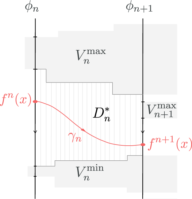
Let
$x \in \mathbb R^2$
 be a point in the plane and let
$O=O(f,x)$
 . For each
$n\in \mathbb Z$
 , let
$\phi _n \in {\mathcal {F}}$
 be the leaf
${\mathcal {F}}$
 containing the point
$f^n(x)$
 . Note that
$(\phi _n)_{n\in \mathbb Z}$
 is a bi-infinite sequence of leaves in
$C_{O}$
 that is increasing with respect to the natural order of the foliation
${\mathcal {F}}$
 , meaning,
$L(\phi _{n+1})\subset L(\phi _n)$
 for all
${n\in \mathbb Z}$
 . Although
${O}$
 must escape to infinity, the sequence
$(\phi _n)_{n\in \mathbb Z}$
 may accumulate at certain leaves of
${\mathcal {F}}$
 . Since
$(\phi _n)_{n\in \mathbb Z}$
 is increasing, there can be two types of leaves accumulated by the sequence
$(\phi _n)_{n\in \mathbb Z}$
 . Either a leaf
$\phi _L\in {\mathcal {F}}$
 , which is a limit leaf of the forward sequence
$(\phi _n)_{n\geq 0}$
 , or a leaf
$\phi _R \in {\mathcal {F}}$
 , which is a limit leaf of the backward sequence
$(\phi _{n})_{n\leq 0}$
 . It is worth noting, since
${\mathcal {F}}$
 is not necessarily Hausdorff, each of these sequences may admit multiple limit leaves.
A priori, each point
$f^n(x) \in {O}$
 can be located anywhere along its underlying leaf
$\phi _n$
 . Hence, in case where the sequence
$(\phi_n)_{n\geq0}$
 converges to a leaf
$\phi _L$
 , the orbit
${O}$
 could possibly exhibit a weird asymptotic behavior with respect to
$\phi _L$
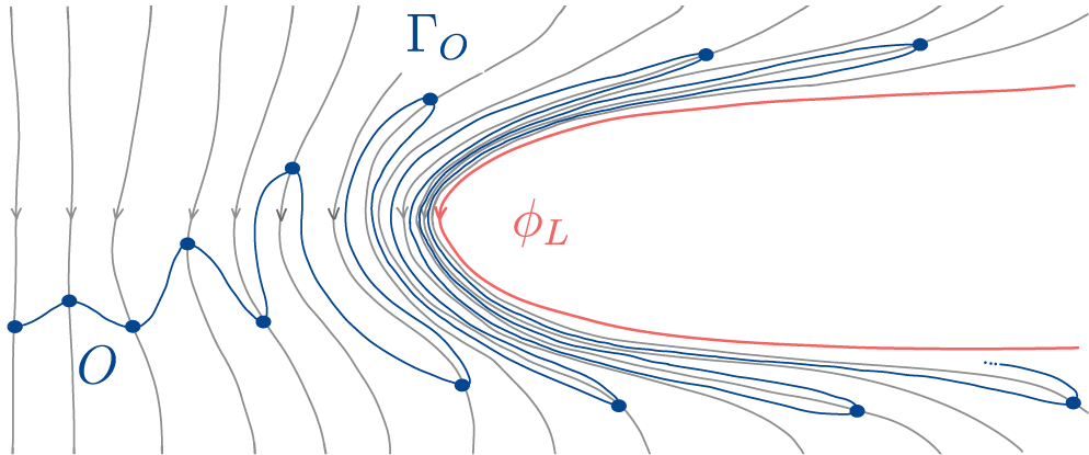
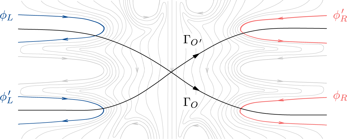
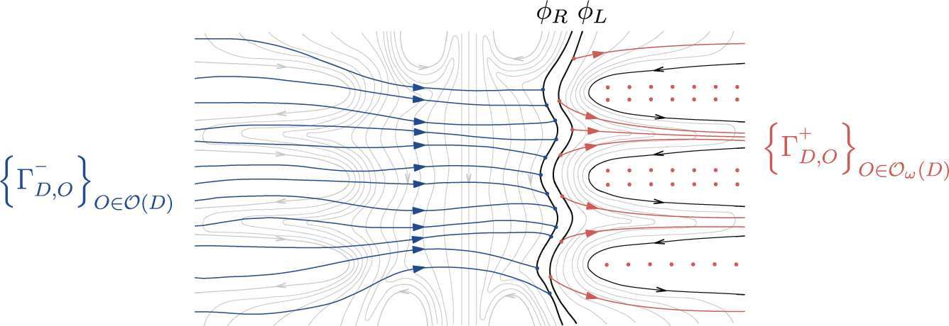
 (see Figure 7) which impedes the existence of properly embedded transverse trajectories of
${O}$
 . Such behavior would pose a significant limitation to the control of topological properties of transverse trajectories.
Weird asymptotic behavior that would make the existence of proper transverse trajectories impossible.

Figure 7 Long description
The diagram illustrates a mathematical vector field using grey lines with downward-pointing arrows.
On the left side, the grey flow lines are nearly vertical. A dark blue line, labeled with a capital O, moves horizontally across these lines in a jagged, oscillating pattern marked by blue circular nodes at each peak and trough.
In the center, the grey flow lines begin to curve around a parabolic region. The blue trajectory, now labeled Gamma sub O, becomes more compressed and follows the curvature of the flow.
On the right side, a smooth red curve labeled phi sub L forms a U-shape opening to the right. The blue trajectory lines become extremely dense and tightly packed as they approach the exterior of this red curve, demonstrating asymptotic behavior where the paths converge but do not cross the red boundary. The grey flow lines in this region follow the outer contour of the red and blue structures.
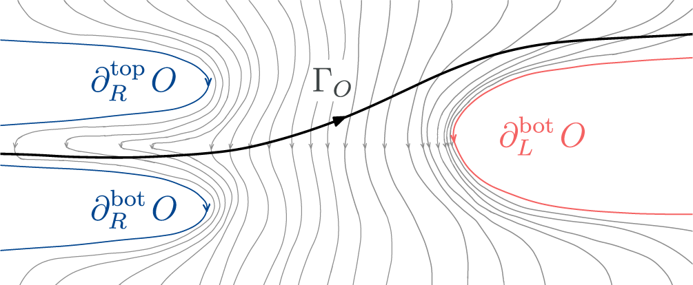
In this section, we overcome this limitation by proving that every orbit of f indeed admits proper transverse trajectories (see Theorem A). Moreover, we show that a proper transverse trajectory
$\Gamma _{O}$
 associated to an orbit
${O}$
 encodes additional information about the asymptotic behavior of
${O}$
 that is not captured by
$C_{O}$
 alone, but rather by
$C_{O}$
 and four distinguished subsets of
$\partial C_{O}$
 , namely
$\partial _L^{\mathrm {top}} {O}$
 ,
$\partial _L^{\mathrm {bot}} {O}$
 ,
$\partial _R^{\mathrm {top}} {O}$
 , and
$\partial _R^{\mathrm {bot}} {O}$
 (see Figure 8).
Description of the information encoded by proper transverse trajectories.

Figure 8 Long description
A vector field diagram with numerous thin grey streamlines flowing horizontally. On the left side, there are two blue U-shaped boundaries. The top blue boundary is labeled partial sub R super top O. The bottom blue boundary is labeled partial sub R super bot O. On the right side, there is a single red U-shaped boundary labeled partial sub L super bot O. A thick black line with a central arrow, labeled Gamma sub O, originates from the left between the two blue boundaries and curves upward to pass between the top blue boundary and the red boundary. The grey streamlines follow a similar flow, curving around the boundaries and converging through the narrow channels between the blue and red regions.
3.2 Crossed leaves and limit leaves
For each orbit
${O} \in \mathrm {Orb}(f)$
 , we define the set

where
$\Gamma _{O}$
 represents any transverse trajectory of
${O}$
 . By abuse of notation, we treat
$C_{O}$
 as a saturated subset of
$\mathbb R^2$
 (see §2.2). According to Lemmas 2.7 and 2.4, the saturated set
$C_{O} \subset \mathbb R^2$
 is a leaf domain of
${\mathcal {F}}$
 and, consequently, it is homeomorphic to a trivially foliated plane, and its boundary
$\partial C_{O}$
 is a locally finite and non-separating collection of leaves in
${\mathcal {F}}$
 . The set
$C_{O}$
 is often referred to as the leaf domain of the orbit
${O}$
 leaves in
$C_{O}$
 are said to be crossed by the orbit
${O}$
 .
Since the set
$C_{O}$
 is a leaf domain, its boundary
$\partial C_{O}$
 admits two distinguished subsets, namely the left-limit and right-limit leaves of
$C_{O}$
 , which are defined as follows:

By fixing a basepoint
$x \in O$
 and considering the bi-infinite sequence
$(\phi _n)_{n\in \mathbb Z}$
 formed by the leaves
$\phi _n \in {\mathcal {F}}$
 passing through the points
$f^n(x)$
 , we note that the forward sequence
$(\phi _n)_{n\geq 0}$
 converges simultaneously to all leaves in
$\partial _L C_{O}$
 (with respect to the quotient topology on
${\mathcal {F}}$
 ), while the backward sequence
$(\phi _n)_{n\leq 0}$
 converges to all leaves in
$\partial _R C_{O}$
 . This can be deduced from the fact that, for any leaf
$\phi \in C_{O}$
 , there exists
$n \geq 0$
 such that
$L(\phi_{-n}) \subset L(\phi) \subset L(\phi_n)$
 . Observe that the sets
$\partial _L C_{O}$
 and
$\partial _R C_{O}$
 are disjoint by definition, and their union may not cover the entire boundary set
$\partial C_{O}$
 (see Figure 1).
Remark 3.1. For any pair of orbits
${O},{O}^{\prime }\in {\mathrm {Orb}}(f)$
 , the following properties hold.
-
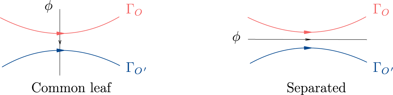
(i) Common leaf versus Separated. The orbits ${O}$
and
${O}^{\prime }$
respect a natural dichotomy: either their
$C_{O}$
and
$C_{{O}^{\prime }}$
intersect, in which case every leaf
${\phi \in C_{O} \cap C_{{O}^{\prime }}}$
is called a common leaf of
${O}$
and
${O}'$
; or sets
$C_{O}$
and
$C_{{O}^{\prime }}$
are disjoint, in which case we say the orbits
${O}$
and
${O}^{\prime }$
are separated, since they are separated by the leaf
$\phi \in \partial C_{O}$
that bounds the connected component of
$\mathbb R^2\setminus C_{O}$
, which contains
$C_{{O}^{\prime }}$
(see Figure 9). -
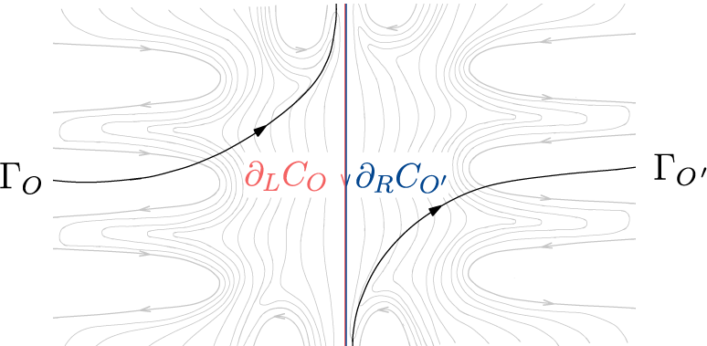
(ii) If $\partial _L C_{O} \cap \partial _R C_{{O}^{\prime }} \neq \varnothing $
, then
$C_{O} {\kern-1pt}\cap{\kern-1pt} C_{{O}^{\prime}} = \varnothing \text{ and } \partial_L C_{O} \cap \partial_R C_{{O}^{\prime}} {\kern-1pt}={\kern-1pt} \{\phi\} $
(Figure 10). -
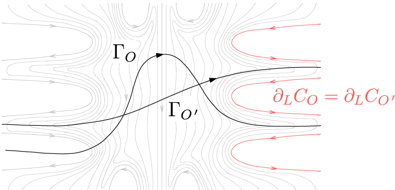
(iii) If $\partial _L C_{O} \cap \partial _L C_{{O}^{\prime }} \neq \varnothing $
, then
$C_{O} \cap C_{{O}^{\prime}} \neq \varnothing \text{ and } \partial_L C_{O} = \partial_L C_{{O}^{\prime}}$
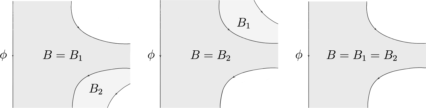
(Figure 11).Figure 9The two possible configurations for pairs of orbits of f with respect to $\mathcal{F}$
.Figure 10Illustration of the property (ii) from Remark 3.1.
Figure 11Illustration of the property (iii) from Remark 3.1.
Figure 11 Long description
A vector field plot features a background of numerous thin grey streamlines that flow vertically near the center and curve horizontally toward the edges. Two prominent black curves with directional arrows intersect in the center. The first curve, labeled Gamma sub O, enters from the bottom left, peaks in the upper center, and exits toward the bottom right. The second curve, labeled Gamma sub O prime, enters from the middle left and follows a more linear path toward the middle right. On the right side of the diagram, three specific streamlines are highlighted in red, forming U-shaped loops that point toward the left. Between these red loops, a mathematical equation is written in red text: partial sub L C sub O equals partial sub L C sub O prime.










3.3 Definition of order
$\prec $
on the sets
$\partial _L C_{O}$
and
$\partial _R C_{O}$


Fix
${O} \in \mathrm {Orb}(f)$
 and a basepoint
$x \in {O}$
 . Since
$\partial C_{O}$
 is a locally finite collection of leaves disjoint from the closed set
$\phi _0 \cup {O}$
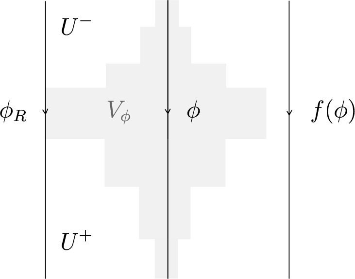
 , we can apply Lemma 2.2 to affirm that there exists a locally finite family
$\{V_\phi \}_{\phi \in \partial C_{O}}$
 of pairwise disjoint closed sets such that, for each
$\phi \in \partial C_{O}$
 , the set
$V_\phi $
 is a trivial neighborhood of
$\phi $
 disjoint from
$\phi _0 \cup {O}$
 .
For each
$n\in \mathbb Z$
 , let
$\phi _n \in {\mathcal {F}}$
 be the leaf passing through the point
$f^n(x)$
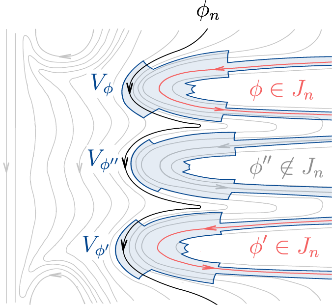
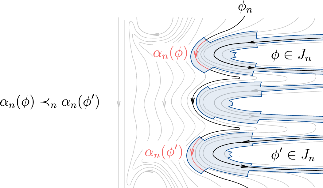
 and define

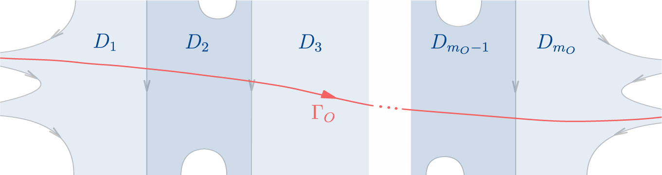
(see Figure 12).
Definition of the sets
$J_n$
 .

Figure 12 Long description
A mathematical diagram illustrating flow lines and regions. On the left, vertical wavy lines represent a vector field. On the right, three horizontal, finger-like lobes extend toward the left.
Top Lobe: Outlined in blue and shaded light blue. A black arrowed line follows the outer curve, labeled V sub phi. Inside the lobe, a red arrowed line loops around the center. The text inside the lobe reads phi is an element of J sub n in red.
Middle Lobe: Outlined in blue and shaded light blue. A black arrowed line follows the outer curve, labeled V sub phi double prime. Inside the lobe, a gray arrowed line loops around the center. The text inside the lobe reads phi double prime is not an element of J sub n in gray.
Bottom Lobe: Outlined in blue and shaded light blue. A black arrowed line follows the outer curve, labeled V sub phi prime. Inside the lobe, a red arrowed line loops around the center. The text inside the lobe reads phi prime is an element of J sub n in red.
A single black line labeled phi sub n at the top center traces the boundary between the vertical flow lines and the tips of the three lobes.
Observe that, by construction,
$J_n \subset \partial _L C_{O}$
 when
$n>0$
 and
$J_n \subset \partial _R C_{O}$
 when
$n<0$
 .
Lemma 3.2. The sequence of sets
$(J_n)_{n\geq 0}$
 forms a filtration of
$\partial _L C_{O}$
 , in the sense that:
-
(i) $J_0 = \varnothing $
; -
(ii) $J_n \subset J_{n+1}$
for any
$n\geq 0$
; -
(iii) $\partial _L C_{O} = \bigcup _{n\geq 0} J^{n}$
.


Similarly, the sequence of sets
$(J_n)_{n\leq 0}$
 forms a filtration of the set
$\partial _R C_{O}$
 .
Proof. We prove the lemma for the sequence
$(J_n)_{n\geq 0}$
 ; the proof for
$(J_n)_{n\leq 0}$
 is analogous.
Since the leaf
$\phi _0$
 is disjoint from each set in the family
$\{V_\phi \}_{\phi \in \partial _L C_{O}}$
 , it holds that
$J_0 = \varnothing $
 . Next, as the sequence of leaves
$(\phi _n)_{n\geq 0}$
 is increasing in
${\mathcal {F}}$
 , if some leaf
$\phi _n$
 intersects
$V_\phi $
 for a given integer
$n \geq 0$
 , then the leaf
$\phi _{n+1}$
 also intersects
$V_\phi $
 . In other words, it holds that

Finally, note that for each leaf
$\phi \in C_{O}$
 , there exists some
$n>0$
 such that
$L(\phi _n) \subset L(\phi )$
 . Therefore, for each
$\phi \in \partial _L C_{O}$
 , there exists the smallest positive integer
$N_\phi>0$
 satisfying

This implies that
$\partial _L C_{O} = \bigcup _{n\geq 0} J^{n}$
 and, thus, we conclude the proof of the lemma.
First, note that for each
$n \in \mathbb Z$
 and
$\phi \in J_n$
 , the set
$\alpha _n(\phi ):=\phi _n \cap V_\phi $
 is a non-empty compact sub-arc of the leaf
$\phi _n$
 . This gives us, for each
$n \in \mathbb Z$
 , a family
$A_n:=\{\alpha _n(\phi )\}_{\phi \in J_n}$
 of pairwise disjoint sub-arcs of the leaf
$\phi _n$
 . Next, note that the orientation of
$\phi _n$
 induces a natural total order on the set
$A_n$
 , which is defined as follows. For any two arcs
$\alpha ,\alpha '\in A_n$
 , we write
$\alpha \prec _n \alpha '$
 if, along the oriented leaf
$\phi _n$
 , the arc
$\alpha '$
 is positioned after
$\alpha $
 . Through the bijection
$\phi \longmapsto \alpha _n(\phi )$
 , we import this order to
$J_n$
 . Given two leaves
$\phi ,\phi '\in J_n$
 , we say that

(see Figure 13).
Definition of the order
$\prec_n$
 on the set
$J_n$
 .

Figure 13 Long description
On the far left, the text alpha sub n (phi) followed by a curly less-than symbol with a subscript n and alpha sub n (phi prime) establishes the ordering rule. To the right, a series of gray contour lines flow vertically and curve around three horizontal, finger-like structures.
* The top structure is shaded light blue and outlined in dark blue. It contains a black U-shaped arrow pointing left then right. Inside the white center of this structure is the label phi is an element of J sub n. A red label alpha sub n (phi) is positioned at the tip of this structure, associated with a red curved arrow.
* The middle structure is similar but lacks specific labels, showing only the black U-shaped directional arrow and gray contour lines.
* The bottom structure is also shaded light blue and contains the label phi prime is an element of J sub n. A red label alpha sub n (phi prime) is at its tip with a corresponding red arrow.
A black line labeled phi sub n at the top right traces the boundary of these structures, separating the blue-shaded regions from the surrounding gray field.
Observe that
$\prec _n$
 and
$\prec _{n+1}$
 are compatible with the inclusion
$J_n \subset J_{n+1}$
 for any
$n\geq 0$
 . This means that, if two leaves
$\phi ,\phi '\in J_n$
 satisfy
$\phi \prec _n \phi '$
 , then they also satisfy
$\phi \prec _{n+1} \phi '$
 . This ensures that the set
$ \partial _L C_{O} = \bigcup _{n>0} J_{n} $
 inherits a total order
$\prec $
 that extends the sets in the filtration
$(J_n)_{n\geq 0}$
 , in the sense that, for any
$\phi ,\phi '\in \partial _L C_{O}$
 , we define the relation

Note that the set
$\partial _R C_{O}$
 inherits an analogous total order
$\prec $
 from the filtration
$(J_n)_{n\leq 0}$
 .
Remark 3.3. There are two important properties of the order
$\prec $
 that we want to highlight.
-
(i) The definition of $\prec $
does not change if the trivial neighborhoods in the family
$\{V_\phi \}_{\phi \in \partial C_{O}}$
are replaced by smaller ones. This ensures that our construction is independent of the choice of trivial neighborhoods, if they are taken small enough; -
(ii) By taking sufficiently small cross-sections $\sigma _\phi \subset V_\phi $
over each leaf
$\phi \in \partial _L C_{O}$
, and then extending them until they reach the leaf
$\phi _0$
, we can obtain a family
$\{\gamma _\phi \}_{\phi \in \partial _L C_{O}}$
of pairwise disjoint paths
$\gamma _\phi :[0,1]\longrightarrow \mathbb R^2$
positively transverse to the foliation
${\mathcal {F}}$
that joins the points
$\gamma _\phi (0) \in \phi _0$
and
$\gamma _\phi (1) \in \phi $
. This allows us to express the order
$\prec $
in terms of the order of the endpoints
$\{\gamma _\phi (0)\}_{\phi \in \partial _L C_{O}}$
along the leaf
$\phi _0$
, meaning that $$ \begin{align*} \phi \prec \phi' \iff \gamma_\phi(0) < \gamma_{\phi'}(0) \text{ according to the orientation of } \phi_0.\end{align*} $$


3.4 Orbit induced cuts
Let
$\text {Cut}_\prec (\partial _L C_{O})$
 be the set of cuts of
$(\partial _L C_{O},\prec )$
 , that is, the set of all pairs
$(A,B)$
 such that
$A, B \subset \partial _L C_{O}$
 are disjoint subsets of
$\partial _L C_{O}$
 satisfying:
-
• $A \cup B = \partial _L C_{O}$
; -
• for any leaf $\phi \in A$
and any leaf
$\phi ' \in B$
, it holds that
$\phi \prec \phi '$
.



Similarly, let
$\text {Cut}_\prec (\partial _R C_{O})$
 denote the set of all cuts of the totally ordered set
$(\partial _R C_{O},\prec )$
 .
Proposition 3.4. Every orbit
${O} \in \mathrm {Orb}(f)$
 admits two canonically defined cuts

The cuts
$(\partial_L^{\mathrm{top}} O,\partial_L^{\mathrm{bot}} O)$
 and
$(\partial_R^{\mathrm{top}} O,\partial_R^{\mathrm{bot}} O)$
 canonically associated to the orbit
$O$
 .

Figure 14 Long description
A line diagram depicting a mathematical vector field with various flow lines and a central orbit.
* On the left side, three blue U-shaped curves with arrows pointing inward are stacked vertically. They are labeled from top to bottom as partial R super top O, partial R super top O, and partial R super bot O.
* In the center, a series of light gray vertical and wavy flow lines run from top to bottom. A diagonal path of black dots, labeled O, crosses from the lower left to the upper right. A gray label C sub O is positioned to the right of the central vertical axis.
* On the right side, three red U-shaped curves with arrows pointing outward are stacked vertically. They are labeled from top to bottom as partial L super top O, partial L super bot O, and partial L super bot O.
* The background consists of thin, light gray contour lines that follow the general flow of the vector field, curving around the blue and red boundary structures.
It is worth remarking that the sets
$\partial _L^{\mathrm {top}} {O}$
 ,
$\partial _L^{\mathrm {bot}} {O}$
 ,
$\partial _R^{\mathrm {top}} {O}$
 , and
$\partial _R^{\mathrm {bot}} {O}$
 depend not only on
${O}$
 , but also on the foliation
${\mathcal {F}}$
 . However, we often omit the dependence on
${\mathcal {F}}$
 in the notation.
The leaf domain
$C_{O}$
 and the cuts
$(\partial _L^{\mathrm {top}} {O},\partial _L^{\mathrm {bot}} {O})$
 and
$(\partial _R^{\mathrm {top}} {O},\partial _R^{\mathrm {bot}} {O})$
 describe the asymptotic behavior of the orbit
${O}$
 with respect to
${\mathcal {F}}$
 (Figure 14). The qualitative data associated with these objects are strictly greater than those given by the set
$C_{O}$
 alone. Throughout this work, we refer to the qualitative data as the
${\mathcal {F}}$
 -asymptotic behavior of
${O}$
 .
Later, in §3.5, we show that the cuts
$(\partial _L^{\mathrm {top}} {O},\partial _L^{\mathrm {bot}} {O})$
 and
$(\partial _R^{\mathrm {top}} {O},\partial _R^{\mathrm {bot}} {O})$
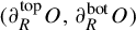 can be interpreted by proper transverse trajectories of
${O}$
 (see Theorem A). These proper transverse trajectories completely describe the
${\mathcal {F}}$
 -asymptotic behavior of the orbit
${O}$
 , differently from arbitrary (non-proper) trajectories, which only encode the information carried by
$C_{O}$
 .
Proof of Proposition 3.4.
Fix an orbit
${O} \in \mathrm {Orb}(f)$
 , a basepoint
$x \in {O}$
 , a family
$\{V_\phi \}_{\phi \in \partial C_{O}}$
 of trivial-neighborhoods, the leaves
$(\phi _n)_{n\in \mathbb Z}$
 , and the sets
$(J_n)_{n\in \mathbb Z}$
 as defined in §3.3.
Observe that, by cutting each leaf
$\phi _n$
 at the point
$f^n(x)$
 , we obtain two half-lines

with endpoints
$\phi ^+_n(0) = \phi ^-_n(0) = f^n(x)$
 and satisfying
$\phi ^+_n, \phi ^-_n \subset \phi _n$
 . Recall that each set in the family
$\{V_\phi \}_{\phi \in \partial C_{O}}$
 is disjoint from the orbit
${O}$
 . Consequently, for each
$n \in \mathbb Z$
 and
$\phi \in J^n$
 , the arc
$\alpha _n(\phi ) := \phi _n \cap V_\phi $
 must lie entirely within one of the two half-lines, either
$\phi _n^+$
 or
$\phi _n^-$
 . This allows us to define, for any
$n \in \mathbb Z$
 , a cut
$(J_n^-,J_n^+) \in \text {Cut}_\prec (J_n)$
 given by the sets

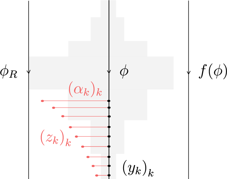
Claim 3.5. For each leaf
$\phi \in \partial _L C_{O}$
 , there exists
$M_\phi>0$
 which is the smallest positive integer such that, for any
$n \geq M_\phi $
 , the following two equivalences hold

Similarly, for each leaf
$\phi \in \partial _R C_{O}$
 , there exists
$M_\phi <0$
 satisfying an analogous property.
Proof of Claim 3.5.
Fix a leaf
$\phi \in \partial _L C_{O}$
 and denote by
$\phi _R \in C_{O}$
 the right-most leaf that intersects the trivial-neighborhood
$V_\phi $
 . The open set
$L(\phi _R) \cap R(\phi )\setminus V_\phi $
 has exactly two connected components, named
$U^+$
 and
$U^-$
 according to the following equivalences:

To simplify the argument, we can profit from Homma–Schoenflies theorem to suppose, up to conjugacy, that the topological lines
$\phi _R$
 ,
$\phi $
 , and
$f(\phi )$
 are verticals on the plane oriented downwards; the set
$U^-$
 lies on the upper half-plane; the set
$U^+$
 lies on the lower half-plane; and that f maps the points of
$\phi $
 into
$f(\phi )$
 as a horizontal (see Figure 15). We represent
$V_\phi $
 disjoint from
$f(\phi )$
 because
$V_\phi $
 is considered small enough; however, our proof does not depend on this property and it is possible that
$V_\phi $
 intersects
$f(\phi )$
 .
Setting in the proof of Claim 3.5 after applying the Homma–Schoenflies theorem.

Now, we suppose by contradiction that the claim of the lemma does not hold. More precisely, we suppose that there exists an increasing sequence of integers
$(n_k)_{k \in \mathbb N}$
 satisfying

According to the equivalence that defines
$U^-$
 and
$U^+$
 , for every
$k \in \mathbb N$
 , it holds that

Since f is a Brouwer homeomorphism,
$(z_k)_{k\in \mathbb N}$
 has no accumulation points on the plane. As the set
$U^+$
 is bounded in the horizontal coordinate and contained in the lower half-plane, the sequence
$(z_k)_{k\in \mathbb N}$
 is unbounded from below on the vertical coordinate. Up to taking a subsequence, we may suppose that
$(z_k)_{k\in \mathbb N}$
 is strictly decreasing on the vertical coordinate. Consequently, the family
$\{\alpha _k\}_{k \in \mathbb N}$
 of horizontal arcs
$\alpha _k$
 that join
$z_k$
 to a point
$y_k \in \phi $
 is, by construction, locally finite (see Figure 16).
Illustration of the family
$\{\alpha_k\}_{k \in \mathbb{N}}$
 of horizontal arcs in the proof of Claim 3.5.

Let
$K\subset \mathbb R^2$
 be the compact arc of zero vertical coordinate connecting
$\phi _R$
 and
$f(\phi )$
 . From the hypothesis given by the Homma–Schoenflies theorem, for any
$k \in \mathbb N$
 , we have that the point
$y_k \in \phi $
 and its image
$f(y_k) \in f(\phi )$
 have exactly the same horizontal coordinate. Consequently, the sequence
$(f(y_k))_{k \in \mathbb N}$
 lies on the lower half-plane, while
$(f(z_k))_{k \in \mathbb N}$
 lies on the upper half-plane. Since the arcs in the family
$\{\alpha _k\}_{k\in \mathbb N}$
 are contained in the set
$\overline {L(\phi _R) \cap R(\phi )}$
 , their images
$\{f(\alpha _k)\}_{k \in \mathbb N}$
 are contained in
$\overline {L(\phi _R) \cap R(f(\phi ))}$
 . Note that, since
$f(\alpha _k)$
 joins the point
$f(y_k)$
 to
$f(z_k)$
 , which are respectively in the lower and upper half-planes, each arc in the family
$\{f(\alpha _k)\}_{k \in \mathbb N}$
 must intersect the compact set K. In other words,
$\{f(\alpha _k)\}_{k \in \mathbb N}$
 is not a locally finite family of arcs (see Figure 17).
Illustration of the family
$\{f(\alpha_k)\}_{k \in \mathbb{N}}$
 of horizontal arcs in the proof of Claim 3.5.

Figure 17 Long description
The diagram is composed of three vertical lines intersected by a central horizontal line.
At the top left, a series of blue dots curves upward, labeled f (z sub k) sub k. A solid blue curve, labeled f (alpha sub k), originates from one of these dots, crosses the central vertical line, and descends to meet the rightmost vertical line.
A light gray shaded region shaped like a stepped cross is centered on the intersection of the middle vertical and horizontal lines, labeled with a capital K.
The horizontal axis is labeled phi sub R on the left and f (phi) on the right.
In the lower-left quadrant, a family of nine thin red horizontal arcs extends from the leftmost vertical line toward the center. Each arc terminates in a small red dot, with the lengths of the arcs decreasing as they move lower.
On the rightmost vertical line, a series of black dots corresponds to the vertical positions of the red arcs and the blue curve, labeled at the bottom as (f (y sub k)) sub k.
However, since f is a homeomorphism and
$\{\alpha _k\}_{k \in \mathbb N}$
 is locally finite,
$\{f(\alpha _k)\}_{k \in \mathbb N}$
 should be, in fact, locally finite. This gives us a contradiction.
Due to Claim 3.5, we can now define the following sets:

By construction, we have that
$(\partial _L^{\mathrm {top}} {O},\partial _L^{\mathrm {bot}} {O}) \in \text {Cut}_\prec (\partial _L C_{O})$
 . We can define the other two sets
$\partial _R^{\mathrm {top}} {O}$
 and
$\partial _R^{\mathrm {bot}} {O}$
 in a similar way, which thus concludes the proof of the proposition.
3.5 Proper transverse trajectories
We now prove Theorem A, which we restate.
Theorem A. Every orbit
${O} \in \mathrm {Orb}(f)$
 admits a proper transverse trajectory. Moreover, any proper transverse trajectory
$\Gamma _{O}$
 associated to the orbit
${O}$
 satisfies the equalities

(see Figure 18).
Depiction of how a proper transverse trajectory
$\Gamma_O$
 of an orbit
$O$
 recovers the cannonically associated cuts
$(\partial_L^{\mathrm{top}} O, \partial_L^{\mathrm{bot}} O)$
 and
$(\partial_R^{\mathrm{top}} O,\partial_R^{\mathrm{bot}} O)$
 , as stated in Theorem A.

Figure 18 Long description
The diagram features a central black curve labeled Gamma sub O with an arrow pointing right, representing a transverse trajectory. This curve passes through a dense field of light gray flow lines that curve vertically in the center and horizontally toward the edges.
On the left side, three blue U-shaped curves represent cuts. They are labeled from top to bottom as:
* partial R super top O
* partial R super top O
* partial R super bot O
On the right side, three red U-shaped curves represent corresponding cuts. They are labeled from top to bottom as:
* partial L super top O
* partial L super bot O
* partial L super bot O
A gray label C sub O is positioned in the lower-right quadrant among the gray flow lines. The flow lines on the far left and far right have small arrows indicating a direction toward the center along the horizontal axis.
Proof. Consider an orbit
${O} \in \mathrm {Orb}(f)$
 , a basepoint
$x \in {O}$
 , a family
$\{V_\phi \}_{\phi \in \partial C_{O}}$
 of trivial neighborhoods, the leaves
$(\phi _n)_{n\in \mathbb Z}$
 , and the sets
$(J_n)_{n\in \mathbb Z}$
 as defined in §3.3. Recall that in the proof of Lemma 3.2 and Proposition 3.4, we defined, for each leaf
$\phi \in \partial _L C_{O}$
 , two integers
$N_\phi>0$
 and
$M_\phi>0$
 , which are the smallest positive integers satisfying

Observe that, for
$n \geq M_\phi $
 , the following two scenarios cannot occur (see Figure 19):

This means that, for each
$n\geq M_\phi $
 , there exists a path
$\gamma _{n,\phi }:[0,1]\longrightarrow \mathbb R^2$
 positively transverse to
${\mathcal {F}}$
 that joins
$f^n(x)$
 to
$f^{n+1}(x)$
 and is disjoint from the neighborhood
$V_\phi $
 .
Illustration of what cannot occur (on the left) and what actually occurs (on the right).

Figure 19 Long description
The diagram consists of two panels side-by-side.
Left Panel: Two vertical black lines are labeled phi sub n on the left and phi sub n plus 1 on the right. A red dot on the left line is labeled f super n (x). A dashed red curve labeled gamma sub n descends from this dot, passing through a central gray shaded region labeled V sub phi, and ends at a red dot on the right line labeled f super n plus 1 (x). Below the panel is the expression phi is an element of J sub n super minus intersection J sub n plus 1 super plus.
Right Panel: Similar vertical lines phi sub n and phi sub n plus 1. A red dot on the left line is labeled f super n (x). A solid red curve labeled gamma sub n with an arrow pointing right connects this dot to a red dot on the right line labeled f super n plus 1 (x). This path stays above the central gray shaded region V sub phi. Below the panel is the expression phi is an element of J sub n super minus intersection J sub n plus 1 super minus.
The first step of the proof is to show that, by modifying the trivial neighborhoods in the family
$\{V_\phi \}_{\phi \in \partial C_{O}}$
 , we can ensure that
$N_\phi = M_\phi $
 for all
$\phi \in \partial C_{O}$
 . Indeed, to show this, one should simply observe that each leaf
$\phi \in \partial _L C_{O}$
 also admits the trivial neighborhood

Thus, by redefining the original
$V_\phi $
 to be instead the newly defined trivial neighborhood
$V^{\prime }_\phi $
 , we automatically get the property that
$N_\phi = M_\phi $
 . Therefore, we conclude that after this redefinition, we know that for each
$n\geq 0$
 and
$\phi \in \partial _L C_{O}$
 , the points
$f^n(x)$
 and
$f^{n+1}(x)$
 can be connected by a path
$\gamma _{n,\phi }$
 positively transverse to
${\mathcal {F}}$
 that is disjoint from
$V_\phi $
 .
Now, the second step of the proof is to show that, for each
$n\geq 0$
 , we can always construct the paths
$\gamma _{n,\phi }$
 so that they are the same among all leaves
$\phi \in \partial _L C_{O}$
 .
For every
$n \geq 0$
 , we define a partition of the set
$A^n=\{\alpha _n(\phi )\}_{\phi \in J_n}$
 given by

The set
$A^n$
 is ordered according to the orientation of the leaf
$\phi _n$
 . Observe that any element in
$A_n^+$
 is greater than any element in
$A_n^-$
 . Now, since the family
$\{V_\phi \}_{\phi \in \partial _L C_{O}}$
 is locally finite, any compact sub-arc of
$\phi _n$
 intersects finitely many arcs of
$A^n$
 . Consequently, if
$A_n^+\neq \varnothing $
 , then there exists a minimal element
$\alpha _n^{{\min }}$
 in
$A_n^+$
 . Similarly, if
$ A_n^-\neq \varnothing $
 , then there exists a maximal element
$\alpha _n^{\mathrm {max}}$
 in
$A_n^-$
 . In the case where
$A_n^+ = \varnothing $
 or
$A_n^- = \varnothing $
 , such arcs are considered empty. Note that the connected component of
$\phi _n\setminus (\alpha _n^{\mathrm {max}} \cup \alpha _n^{\mathrm {min}})$
 that contains
$f^n(x)$
 intersects no trivial neighborhood in
$\{V_\phi \}_{\phi \in J^n}$
 . For each
$n \geq 0$
 , let
$V_n^{\mathrm {max}}$
 and
$V_n^{\mathrm {min}}$
 be the trivial neighborhoods in the family
$\{V_\phi \}_{\phi \in J^n}$
 containing
$\alpha _n^{\mathrm {max}}$
 and
$\alpha _n^{\mathrm {min}}$
 , respectively.
For each
$n\geq 0$
 , we define the set
$ D_n := \overline {L(\phi _n) \cap R(\phi _{n+1})}.$
 After the redefinition of the trivial neighborhoods as
$V^{\prime }_\phi := V_\phi \cap \overline {L(\phi ^{M_\phi })}$
 in (3.1), only two scenarios are possible:
-
(1) either $V_n^{\mathrm {max}} = V_{n+1}^{\mathrm {max}}$
; -
(2) or the intersection $V_{n+1}^{\mathrm {max}} \cap D_n$
is contained in
$\phi _{n+1}$
.


These scenarios are respectively illustrated in Figure 20. Observe that, if the trivial neighborhood
$V_{n+1}^{\mathrm {max}}$
 is distinct from
$V_n^{\mathrm {max}}$
 , then it must stop at the leaf
$\phi _{n+1}$
 . This is also a consequence of the redefinition in (3.1), as it implies that
$V_\phi \subset \overline {L(\phi ^{M_\phi })}$
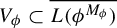 .
Illustration of scenarios (1) and (2) after redefining
$V'_\phi:= V_\phi \cap \overline {L(\phi ^{M_\phi })}$
 .

We have completely analogous alternatives for the sets
$V_n^{\mathrm {min}}$
 for all
$n \geq 0$
 .
Either way, for each
$n\geq 0$
 , we have that the points
$f^n(x)$
 and
$f^{n+1}(x)$
 are contained in the same connected component, namely
$D^*_n$
 (see Figure 21), of the set

This further implies that, for each
$n \geq 0$
 , the points
$f^n(x)$
 and
$f^{n+1}(x)$
 can be connected via a path
$\gamma _n:[0,1]\longrightarrow \mathbb R^2$
 that is positively transverse to
${\mathcal {F}}$
 and contained in
$D^*_n$
 . Therefore, since
$\gamma _n \subset D^*_n$
 , it follows that
$\gamma _n$
 is disjoint from every set in the family
$\{V_\phi \}_{\phi \in \partial _L C_{O}}$
 .
Illustration describing the properties of the set
$D^*_n$
 .

Figure 21 Long description
Two parallel vertical lines serve as the primary axes. The left axis is labeled phi sub n at the top and the right axis is labeled phi sub n plus 1 at the top.
Between these axes, three distinct regions are defined vertically.
1. The top region is a light gray shaded area labeled V sub n super max.
2. The middle region is a white area filled with thin vertical gray lines, labeled D sub n asterisk.
3. The bottom region is a light gray shaded area labeled V sub n super min.
A red curved path, labeled gamma sub n, originates from a red dot on the left axis labeled f super n (x). The path curves downward and to the right, ending at a red dot on the right axis labeled f super n plus 1 (x).
On the right axis, a specific vertical segment within the middle region is marked with tick marks and labeled V sub n plus 1 super max. Both vertical axes feature downward-pointing arrowheads indicating a directional flow.
By repeating the same construction with respect to the set
$\partial _R C_{O}$
 , we end up with a family of positively transverse paths
$\{\gamma _n\}_{n\in \mathbb Z}$
 , where each
$\gamma _n$
 connects
$ f^n(x)$
 to
$ f^{n+1}(x)$
 , and is disjoint from
$V_{\phi }$
 for any leaf
$\phi \in \partial _L C_{O} \cup \partial _R C_{O}$
 .
Finally, the last step is to prove that the family
$\{\gamma _n\}_{n\in \mathbb Z}$
 is locally finite. For that, define

and observe that every point
$z \in W$
 has an open neighborhood
$U_z\subset \mathbb R^2$
 that intersects finitely many sets in the family
$\{D_n\}_{n \in \mathbb Z}$
 . In particular, each neighborhood
$U_z$
 intersects finitely many paths in the family
$\{\gamma _n\}_{n\in \mathbb Z}$
 . Let
$K \subset \mathbb R^2$
 be a compact set and denote

Note that
$K^*$
 is a compact set contained in W satisfying
$\gamma _n \cap K = \gamma _n \cap K^*$
 for all
$n \in \mathbb Z$
 . Consider a cover of
$K^*$
 of the form
$\{U_z\}_{z \in K^*}$
 . By taking a finite sub-cover, we conclude that
$K^*$
 intersects at most finitely many transverse paths in
$\{\gamma _n\}_{n\in \mathbb Z}$
 . Hence, K intersects finitely many paths in
$\{\gamma _n\}_{n\in \mathbb Z}$
 . This shows that
$\{\gamma _n\}_{n\in \mathbb Z}$
 is a locally finite family and thus

is a properly embedded transverse trajectory associated to
${O}$
 .
The fact that
$\Gamma _{O}$
 satisfies
$\partial _L^{\mathrm {top}} {O} = \partial _L C_{O} \cap L(\Gamma _{O})$
 and
$\partial _L^{\mathrm {bot}} {O} = \partial _L C_{O} \cap R(\Gamma _{O})$
 follows directly from the construction. The analogous properties for
$\partial _R^{\mathrm {top}} {O}$
 and
$\partial _R^{\mathrm {bot}} {O}$
 hold as well. To see that these equalities hold for any proper transverse trajectory
$\Gamma _{O}$
 , it suffices to note that they hold automatically if the trivial neighborhoods in the family
$\{V_\phi \}_{\phi \in \partial C_{O}}$
 are disjoint from
$\Gamma _{O}$
 . Since, in the proper case,
$\Gamma _{O}\subset \mathbb R^2$
 is a closed set disjoint from
$\partial C_{O}$
 , Lemma 2.2 ensures that such a family
$\{V_\phi \}_{\phi \in \partial C_{O}}$
 exists. This concludes the proof.
3.6 Equivalence classes of
${\mathcal {F}}$
-asymptotic orbits

As presented in Definition 1.2, we can relate orbits exhibiting similar
${\mathcal {F}}$
 -asymptotic behavior via equivalence relations
$\stackrel {+}{\sim }$
 and
$\stackrel {-}{\sim }$
 on the set
$\mathrm{orb}$
 . Below, we interpret these relations in terms of proper transverse trajectories.
Lemma 3.6. For any
$ {O},{O}^{ \prime } \in \mathrm {Orb}(f)$
 , the following statements are equivalent:
-
(i) the orbits ${O}$
and
${O}^{\prime }$
are forward
${\mathcal {F}}$
-asymptotic, that is,
${O} \stackrel {+}{\sim } {O}^{ \prime }$
; -
(ii) there exist proper transverse trajectories $\Gamma _{O}$
and
$\Gamma _{{O}^{ \prime }}$
of
${O}$
and
${O}^{ \prime }$
, respectively, such that
$ \Gamma _{O}([ t, \infty )) \cap \Gamma _{{O}^{ \prime }}([ t, \infty )) \neq \varnothing $
for every
$t \in \mathbb R$
(Figure 22).


We can obtain a similar result for the relation
$\stackrel {-}{\sim }$
 by replacing
$[ t, \infty )$
 with
$(-\infty , t ]$
 .
Existence of ‘forever intersecting’ proper trajectories for pairs of
$\mathcal{F}$
 -asymptotic orbits.

Figure 22 Long description
A line graph depicting mathematical trajectories in a flow field. On the left, two primary paths are labeled. A red line, Gamma sub O prime, starts at the top left and curves downward. A blue line, Gamma sub O, starts at the bottom left and curves upward. Both lines have directional arrows pointing toward the center.
In the middle, the red and blue lines intersect and begin to oscillate around each other. They are surrounded by numerous thin grey vertical lines that curve inward toward the center, representing a vector field or flow.
On the right, the oscillating red and blue lines enter a narrow horizontal corridor defined by two thick black parabolic curves.
- The upper curve is labeled partial sub L super top C sub O equals partial sub L super top C sub O prime.
- The lower curve is labeled partial sub L super bot C sub O equals partial sub L super bot C sub O prime.
The red and blue trajectories continue to intertwine in a ‘forever intersecting’ pattern as they move toward the right edge of the frame within these boundaries.
Lemma 3.6 admits a dual version which is slightly stronger, presented in Lemma 3.7.
Lemma 3.7. For any
$ {O},{O}^{\prime } \in {\mathrm {Orb}}(f)$
 satisfying
$C_{O} \cap C_{{O}^{\prime }}\neq \varnothing $
 , the following are equivalent:
-
(i) the orbits ${O}$
and
${O}^{\prime }$
are not forward
${\mathcal {F}}$
-asymptotic, that is,
${O} \not\stackrel{+}{\sim} {O}^{ \prime }$
; -
(ii) for any pair of proper transverse trajectories $\Gamma _{O}$
and
$\Gamma _{{O}^{ \prime }}$
of
${O}$
and
${O}^{ \prime }$
, respectively, there exists
$\phi _L \in C_{O} \cap C_{{O}^{\prime }}$
such that
$\Gamma _{O} \cap \Gamma _{{O}^{ \prime }} \cap \overline {L(\phi _L)} = \varnothing $
(Figure 23).


We obtain a similar result for non-backward
${\mathcal {F}}$
 -asymptotic orbits by replacing each L with R.
Forced divergence for any pair of proper transverse trajectories associated to non-
$\mathcal{F}$
 -asymptotic orbits.

Figure 23 Long description
A two-panel diagram illustrating dynamical systems.
Left Panel: Labeled O not-asymptotic to O prime. A background of light gray streamline curves flows horizontally. A thick black vertical wavy line labeled phi sub R divides the space. Two colored trajectories enter from the left. A red line labeled Gamma sub O starts straight, crosses phi sub R, and then oscillates with decreasing amplitude. A blue line labeled Gamma sub O prime starts below the red line, crosses phi sub R, and then oscillates above the red line before converging toward it.
Right Panel: Labeled O not-asymptotic to O prime with a plus superscript. This panel is a mirrored version of the first. A thick black vertical wavy line is labeled phi sub L. The red trajectory Gamma sub O and blue trajectory Gamma sub O prime enter from the left as oscillating lines that cross the phi sub L boundary and then flatten into straight horizontal lines on the right side.
In both panels, arrows on the colored lines indicate the direction of flow from left to right, and arrows on the black boundary lines point downward.
Remark 3.8. It is important to remark that the results of Lemmas 3.6 and 3.7 are no longer true if we consider non-proper transverse trajectories as in the following example.
We suppose that
${O},{O}^{ \prime } \in \mathrm {Orb}(f)$
 are two orbits admitting a leaf
$\phi \in \partial _L^{\mathrm {top}} {O} \cap \partial _L^{\mathrm {bot}} {{O}^{ \prime }}$
 . These orbits are clearly not forward
${\mathcal {F}}$
 -asymptotic. However, as one can see in Figure 24, there still exist non-proper transverse trajectories
$\Gamma _{O}$
 and
$\Gamma _{{O}^{ \prime }}$
 associated to
${O}$
 and
${O}^{\prime }$
 , respectively, that satisfy the property
$ \Gamma _{O}([ t, \infty )) \cap \Gamma _{{O}^{ \prime }}([ t, \infty )) \neq \varnothing $
 for any
$t \in \mathbb R$
 .
Illustration of the example described in Remark 3.8.

Figure 24 Long description
The diagram illustrates a mathematical flow field.
* Background: Vertical grey lines with downward-pointing arrows represent a steady flow field across the entire frame.
* Central Feature: A large parabolic black outline on the right side contains the mathematical expression partial sub L super top O intersection partial sub L super bot O prime.
* Red Boundary: A smooth red curve labeled Gamma sub O prime slopes upward from the left toward the top right. It features several red circular nodes where it intersects with blue lines.
* Blue Boundary: A jagged blue curve labeled Gamma sub O runs generally below the red curve. It consists of sharp peaks that touch the red curve at the red nodes and deep troughs marked by blue circular nodes.
* Interaction: Between the red curve and the parabolic black boundary, the blue lines become highly concentrated and compressed, following the contour of the parabola before branching out toward the bottom right.
* Points of Interest: On the far left, the blue curve oscillates independently with blue nodes at its base. As it moves right, the peaks of the blue curve align perfectly with the red nodes on the Gamma sub O prime curve.
Proof of Lemma 3.6.
(i)
$\implies $
 (ii): From statement (i), we have
$C_{O} \cap C_{{O}^{ \prime }}\neq \varnothing $
 and
$\partial _L C_{O} = \partial _L C_{{O}^{ \prime }}$
 . Let
$\phi _* \in C_{O} \cap C_{{O}^{ \prime }}$
 and let
$(\phi _n)_{n\geq 0}$
 be the increasing sequence of leaves in
${\mathcal {F}}$
 formed by the leaves intersecting the set
$({O}\cup {O}^{ \prime })\cap \overline {L(\phi _*)}$
 . Note that some leaves of
$(\phi _n)_{n\geq 0}$
 may intersect simultaneously both orbits
${O}$
 and
${O}^{ \prime }$
 . Next, according to Lemma 2.2, there exists a family of sufficiently small trivial neighborhoods
$\{V_\phi \}_{\phi \in \partial _L C_{O}}$
 of the leaves in
$\partial _L C_{O}$
 that is pairwise disjoint and disjoint from the closed set
$\phi _0 \cup {O} \cup {O}^{ \prime }$
 .
Similarly to §3.3, we have a filtration
$(J_n)_{n\geq 0}$
 of the set
$\partial _L C_{O}$
 by sets of the form
$J_n=\{\phi \in \partial _L C_{O} \mid V_\phi \cap \phi _n\}$
 . Moreover, for each
$n\geq 0$
 such that
${O} \cap \phi _n \neq \varnothing $
 , we have a cut

However, for the values of
$n\geq 0$
 such that
${O} \cap \phi _n = \varnothing $
 , we define
$m(n)>n$
 as the smallest integer such that
${O} \cap \phi _{m(n)} \neq \varnothing $
 , and we set

Performing the same adaptation for the cuts induced by the orbit
${O}^{ \prime }$
 , we end up with two cuts
$(J_n^-({O}), J_n^+({O}))$
 and
$(J_n^-({O}^{ \prime }), J_n^+({O}^{ \prime }))$
 of the ordered set
$(J_n,\prec )$
 for every
$n\geq 0$
 .
Since
${O}\stackrel {+}{\sim }{O}^{ \prime }$
 for each leaf
$\phi \in \partial _L C_{O}$
 , there exists
$M_\phi>0$
 such that

By the same redefinition of the family
$\{V_\phi \}_{\phi \in \partial _L C_{O}}$
 presented in (3.1), we can ensure that each leaf
$\phi \in \partial _L C_{O}$
 satisfies
$\phi \not \in J_n$
 for all
$n<M_\phi $
 and, consequently, for any
$n\geq 0$
 , we have

For each
$n\geq 0$
 , let
$p_n$
 and
$p_n'$
 be the points where the leaf
$\phi _n$
 intersects
${O}$
 and
${O}^{ \prime }$
 , respectively. In the case where
$\phi _n$
 intersects only one of these orbits, we consider
$p_n = p_n'$
 . Following arguments similar to those in the proof of Theorem A, we obtain for each
$n\geq 0$
 , two positively transverse paths
$\gamma _n, \gamma _n':[0,1]\longrightarrow \mathbb R^2$
 that are disjoint from all sets in the family
$\{V_\phi \}_{\phi \in \partial _L C_{O}}$
 and such that
$\gamma ^n_{O}(0) = p_n$
 ,
$\gamma ^n_{{O}^{ \prime }}(0) = p_n'$
 ,
$\gamma ^n_{O}(1) = p_{n+1}$
 , and
$\gamma ^n_{{O}^{ \prime }}(1) = p_{n+1}'$
 . Observe that
$p_n$
 ,
$p_n'$
 ,
$p_{n+1}$
 , and
$p_{n+1}'$
 belong to the same connected component of the set

Therefore, for any pair of open sets
$U_n, U_{n+1}\subset \mathbb R^2$
 satisfying
$\phi _n \subset U_n$
 and
$\phi _{n+1} \subset U_{n+1}$
 , the same arguments of §3.5 allow us to construct
$\gamma _n$
 and
$\gamma _n'$
 in such a way that they coincide outside the neighborhoods
$U_n$
 and
$U_{n+1}$
 . Moreover, in the case where
$p_n = p_n'$
 and
$p_{n+1} = p_{n+1}'$
 , we can assume that
$\gamma _n = \gamma _n'$
 . In all cases, we have
$\gamma _n \cap \gamma _n' \neq \varnothing $
 for all
$n\geq 0$
 . The argument of §3.5 proves that the families
$\{\gamma _n\}_{n\geq 0}$
 and
$\{\gamma _n'\}_{n\geq 0}$
 are both locally finite. Thus, they can be concatenated, and then extended, into proper transverse trajectories
$\Gamma $
 and
$\Gamma '$
 associated respectively to the orbits
${O}$
 and
${O}^{ \prime }$
 . These proper transverse trajectories satisfy statement (ii).
(ii)
$\implies $
 (i). Since
$\Gamma $
 and
$\Gamma '$
 intersect each other, there exists a leaf
$\phi _0 \in C_{O} \cap C_{{O}^{ \prime }}$
 . Let
$(\phi _n)_{n\geq 0}$
 be the increasing sequence of leaves in
${\mathcal {F}}$
 formed by the leaves meeting the set
$({O}\cup {O}^{ \prime })\cap \overline {L(\phi _0)}$
 . Since
$\Gamma $
 and
$\Gamma '$
 are proper lines, the set
$\Gamma \cup \Gamma ' \subset \mathbb R^2$
 is closed. Thus, by applying Lemma 2.2, we know there exists a family
$\{V_\phi \}_{\phi \in \partial _L C_{O}}$
 of pairwise disjoint trivial neighborhoods of
$\partial _L C_{O}$
 that satisfies
$V_\phi \cap (\phi _0 \cup \Gamma \cup \Gamma ') = \varnothing $
 for any
$\phi \in \partial _L C_{O}$
 .
For each
$n\geq 0$
 , we consider
$J_n=\{\phi \in \partial _L C_{O} \mid V_\phi \cap \phi _n\}$
 . As in (i)
$\implies $
 (ii), consider the sets
$J_n^- ({O})$
 ,
$J_n^+ ({O})$
 ,
$J_n^-({O}^{ \prime })$
 , and
$J_n^+({O}^{ \prime })$
 . Note that, as each
$V_\phi $
 is disjoint from
${\Gamma \cup \Gamma '}$
 , hypothesis (ii) implies that,
$\text {for all } n\geq 0$
 , we have
$J_n^+ ({O}) = J_n^+ ({O}^{ \prime }) $
 and
$J_n^- ({O}) = J_n^- ({O}^{ \prime })$
 . This shows that the orbits
${O}$
 and
${O}^{ \prime }$
 induce the same cut
$(\partial _L^{\mathrm {top}} {O}, \partial _L^{\mathrm {bot}}{O})$
 on
$\partial _L C_{O}$
 and, consequently, we conclude that
${O}$
 and
${O}^{ \prime }$
 are forward
${\mathcal {F}}$
 -asymptotic.
Remark 3.9. The argument (i)
$\implies $
 (ii) within the proof of Lemma 3.6 can be adapted to any finite subset
${\mathcal {O}}\subset \mathrm {Orb}(f)$
 satisfying

If each leaf of
${\mathcal {F}}$
 intersects at most one orbit in
${\mathcal {O}}$
 , this adaptation proves Lemma 7.2.
Proof of Lemma 3.7.
(i)
$\implies $
 (ii). Suppose that
${O} \not\stackrel{+}{\sim} {O}^{ \prime }$
 . According to Lemma 3.6, for any pair of proper transverse trajectories
$\Gamma _{O}$
 and
$\Gamma _{{O}^{ \prime }}$
 of
${O}$
 and
${O}^{ \prime }$
 , there exists
$M>0$
 such that

Since
$\Gamma _{O}$
 and
$\Gamma _{{O}^{ \prime }}$
 are topological lines, the intersection
$\Gamma _{O} \cap \Gamma _{{O}^{ \prime }}$
 is a closed subset of
$\mathbb R^2$
 . Therefore, the set
$ {\Gamma _{O}}^{-1}(\Gamma _{O} \cap \Gamma _{{O}^{ \prime }})$
 is a closed subset of
$\mathbb R$
 bounded from above by M and, consequently, it admits a maximal element
$t_{\mathrm {max}}$
 .
Note that the leaf
$\phi _{\mathrm {max}}\in {\mathcal {F}}$
 passing through the point
$\Gamma _{O}(t_{\mathrm {max}})$
 belongs to
$C_{O} \cap C_{{O}^{ \prime }}$
 . Since
$C_{O} \cap C_{{O}^{ \prime }}$
 is an open set, there exists a leaf
$\phi _L\in {\mathcal {F}}$
 satisfying
$L(\phi _L) \subset L(\phi _{\mathrm {max}})$
 and sufficiently close to
$\phi _{\mathrm {max}}$
 so that it also belongs to
$C_{O} \cap C_{{O}^{ \prime }}$
 . This leaf proves (i)
$\implies $
 (ii).
(ii)
$\implies $
 (i). This implication follows trivially by Lemma 3.6.
4 Sided preorders of orbits
In this section, we develop the tools necessary to compare orbits which cross a common leaf and exhibit distinct
${\mathcal {F}}$
 -asymptotic behaviors.
We are motivated by the setting below.
Let
${O}, {O}^{\prime } \in \mathrm {Orb}(f)$
 be orbits crossing a common leaf, i.e.
$C_{O} \cap C_{{O}^{\prime }} \neq \varnothing $
 . Suppose that
${O}$
 and
${O}^{\prime }$
 are neither forward nor backward
${\mathcal {F}}$
 -asymptotic. Thus, according to Lemma 3.7, for any proper transverse trajectories
$\Gamma _{O}$
 and
$\Gamma _{{O}^{\prime }}$
 associated with
${O}$
 and
${O}^{\prime }$
 , respectively, there exists a pair of leaves
$\phi _R, \phi _L \in C_{O} \cap C_{{O}^{\prime }}$
 satisfying
$\phi _R < \phi _L$
 such that

In this setting, two possible configurations arise (see Figure 25).
-
(a) The points $p_L({O}) \in \Gamma _{O} \cap \phi _L$
and
$p_L({O}^{\prime }) \in \Gamma _{{O}^{\prime }} \cap \phi _L$
are ordered along the leaf
$\phi _L$
in the same order as the points
$p_R({O}) \in \Gamma _{O} \cap \phi _R$
and
$p_R({O}^{\prime }) \in \Gamma _{{O}^{\prime }} \cap \phi _R$
along
$\phi _R$
. -
(b) The points $p_L({O}) \in \Gamma _{O} \cap \phi _L$
and
$p_L({O}^{\prime }) \in \Gamma _{{O}^{\prime }} \cap \phi _L$
are ordered along the leaf
$\phi _L$
in the opposite order as the points
$p_R({O}) \in \Gamma _{O} \cap \phi _R$
and
$p_R({O}^{\prime }) \in \Gamma _{{O}^{\prime }} \cap \phi _R$
along
$\phi _R$
.


In §4.1, we show that the configuration into which these orbits
${O}$
 and
${O}^{\prime }$
 fall depends solely on their
${\mathcal {F}}$
 -asymptotic behavior, not on the particular choices of proper transverse trajectories
$\Gamma _{O}$
 and
$\Gamma _{{O}^{\prime }}$
 . This is not the case if
$O\stackrel{+}{\sim} {O}^{\prime }$
 or
$O\stackrel{-}{\sim} {O}^{\prime }$
 .
Observe that, in configuration (b), the trajectories
$\Gamma $
 and
$\Gamma '$
 are forced to intersect each other in between the leaves
$\phi _R$
 and
$\phi _L$
 . In configuration (a),
$\Gamma $
 and
$\Gamma '$
 could be disjoint.
4.1 Defining
$\lesssim _L$
and
$\lesssim _R$


In this section, we will define two relations
$\lesssim _L$
 and
$\lesssim _R$
 on the set of orbits
$\mathrm {Orb}(f)$
 that satisfy the following properties.
-
• For each $\phi \in {\mathcal {F}}$
, the relations
$\lesssim _L$
and
$\lesssim _R$
are total preorder on the set $$ \begin{align*} \mathrm{Orb}(\phi) :=\{O \in \mathrm{orb} \mid \phi \in C_{O} \}. \end{align*} $$
-
• For any pair of orbits ${O}, {O}^{\prime } \in {\mathrm {Orb}}(f)$
, the following equivalences hold: $$ \begin{align*} {O}\stackrel{+}{\sim} {O}^{\prime} \iff {O} \lesssim_L {O}^{\prime} \quad \text{and}\quad {O}^{\prime} \lesssim_L {O}, \\ {O}\stackrel{-}{\sim} {O}^{\prime} \iff {O} \lesssim_R {O}^{\prime} \quad \text{and}\quad {O}^{\prime} \lesssim_R {O}. \end{align*} $$


Before, we note that
$C_{O} \cap C_{{O}^{\prime }}$
 is a (possibly empty) leaf domain of
${\mathcal {F}}$
 (see Lemma 2.6). Moreover, limit sets
$\partial _L(C_{O} \cap C_{{O}^{\prime }})$
 and
$\partial _R(C_{O} \cap C_{{O}^{\prime }})$
 are totally ordered by a relation
$\prec $
 , just as for
$\partial _L C_{O}$
 and
$\partial _R C_{O}$
 (see §3.3). This allows us to introduce the next definition.
Two possible configurations at infinity for pairs of orbits
$O$
 and
${O}^{\prime }$
 that cross a common leaf but are neither forward
$\mathcal{F}$
 -asymptotic nor backward
$\mathcal{F}$
 -asymptotic.

Figure 25 Long description
The figure consists of two panels, a and b, each displaying a dense field of light gray flow lines representing a foliation. Two vertical, wavy black lines divide each panel into three regions.
In panel a, two specific orbits are highlighted. A red orbit labeled Gamma sub O prime enters from the top-left, crosses the first vertical line, and exits at the top-right. A blue orbit labeled Gamma sub O enters from the bottom-left, crosses the first vertical line, and exits at the bottom-right. The orbits are roughly parallel and do not converge.
In panel b, the configuration changes. The red orbit Gamma sub O prime enters from the top-left but, after crossing the vertical lines, it exits at the bottom-right. Conversely, the blue orbit Gamma sub O enters from the bottom-left and exits at the top-right. This creates a crossing pattern where the orbits swap their vertical positions relative to each other as they pass through the central region. Small arrows on the colored lines indicate the direction of the flow from left to right.
Definition of
$\lesssim_{R}$
 and
$\lesssim_{L}$
 .

Figure 26 Long description
The diagram consists of eight panels arranged in two columns. The left column is headed by the relation O less-than-or-equal-to sub R O prime, and the right column by O less-than-or-equal-to sub L O prime. Each panel contains a mathematical definition followed by a vector field diagram.
* Left Column (R-series):
- (R1): Defines conditions for phi and phi prime in the boundary of the intersection of C sub O and C sub O prime. The diagram shows two black U-shaped boundaries on the left with flow lines converging toward a central crossing of a red line Gamma sub O and a blue line Gamma sub O prime.
- (R2): Defines a leaf phi in the boundary. The diagram shows a single black U-shaped boundary on the left with the red line Gamma sub O passing above it and the blue line Gamma sub O prime below it.
- (R3): Similar to R2 but focuses on leaf phi prime. The diagram shows the black U-shaped boundary on the left with the blue line Gamma sub O prime passing through its center.
- (R4): Defines boundary equality and subset relations. The diagram shows a single black U-shaped boundary on the left with flow lines spreading outward toward the right.
* Right Column (L-series):
- (L1): Mirror image of R1. The black U-shaped boundaries are on the right side of the panel. The red line Gamma sub O and blue line Gamma sub O prime cross in the center.
- (L2): Mirror image of R2. The black U-shaped boundary is on the right. The red line Gamma sub O originates from the right boundary area.
- (L3): Mirror image of R3. The black U-shaped boundary is on the right with the blue line Gamma sub O prime originating from it.
- (L4): Mirror image of R4. The black U-shaped boundary is on the right with flow lines converging into it from the left.
In all diagrams, light gray lines represent the background vector field flow, while red and blue lines represent specific orbits Gamma sub O and Gamma sub O prime respectively.
Definition 4.1. For any
${O}, {O}^{\prime } \in {\mathrm {Orb}}(f)$
 , we define
$\lesssim_{R}$
 and
$\lesssim_{L}$
 as in Figure 26.
Proposition 4.2. The relations
$\lesssim _L$
 and
$\lesssim _R$
 satisfy the following properties.
-
(i) Both relations $\lesssim _L$
and
$\lesssim _R$
are total preorders on the set
$\mathrm {Orb}(\phi )$
for every
$\phi \in {\mathcal {F}}$
. -
(ii) For any pair of orbits ${O}, {O}^{\prime } \in \mathrm {Orb}(f)$
, the following equivalences hold: $$ \begin{align*} {O}\stackrel{+}{\sim} {O}^{\prime} \iff {O} \lesssim_L {O}^{\prime} \quad\text{and}\quad {O}^{\prime} \lesssim_L {O}, \\ {O}\stackrel{-}{\sim} {O}^{\prime} \iff {O} \lesssim_R {O}^{\prime} \quad\text{and}\quad {O}^{\prime} \lesssim_R {O}. \end{align*} $$


Remark 4.3. The result of Proposition 4.2 is equivalent to say that
$\lesssim _L$
 and
$\lesssim _R$
 induce total orders on the quotient sets
$\mathrm {Orb}(\phi )/{\stackrel {+}{\sim }}$
 and
$\mathrm {Orb}(\phi )/{\stackrel {-}{\sim }}$
 , respectively. More precisely:
-
• for $[{O}]^+ , [{O}^{\prime }]^+ \in \mathrm {Orb}(\phi )/{\stackrel {+}{\sim }}$
we have
$[{O}]^+ \lesssim _L [{O}^{\prime }]^+$
whenever
${O} \lesssim _L {O}^{\prime }$
; -
• for $[{O}]^- , [{O}^{\prime }]^-\in \mathrm {Orb}(\phi )/{\stackrel {-}{\sim }}$
we have
$[{O}]^- \lesssim _R [{O}^{\prime }]^-$
whenever
${O} \lesssim _R {O}^{\prime }$
.


Proof of Proposition 4.2.
Before we prove item (i), observe that any two orbits
${O}$
 and
${O}^{\prime }$
 that are comparable under
$\lesssim _L$
 (or
$\lesssim _R$
 ) must satisfy
$ C_{O} \cap C_{{O}^{\prime }} \neq \varnothing $
 . The converse statement proves that
$\lesssim _L$
 and
$\lesssim _R$
 are total relations on the subsets
$\mathrm {Orb}(\phi ) \subset \mathrm {Orb}(f)$
 for every
$\phi \in {\mathcal {F}}$
 .
Proof of item (i). Let
${O}, {O}^{\prime } \in \mathrm {Orb}(f)$
 be two orbits satisfying the condition
$C_{O} \cap C_{{O}^{ \prime }} \neq \varnothing $
 . Note that each of the orbits
${O}$
 and
${O}^{ \prime }$
 is allowed to cross at most two leaves in
$\partial (C_{O} \cap C_{{O}^{ \prime }})$
 , one contained in
$\partial _R (C_{O} \cap C_{{O}^{ \prime }})$
 and one in
$\partial _L (C_{O} \cap C_{{O}^{ \prime }})$
 . Moreover, no leaf in
$\partial (C_{O} \cap C_{{O}^{ \prime }})$
 can be crossed simultaneously by
${O}$
 and
${O}^{ \prime }$
 . Based on these observations, we conclude that the orbits
${O}$
 and
${O}^{\prime }$
 must satisfy one of the following.
-
(1) The orbits ${{O}}$
and
${{O}^{ \prime }}$
cross distinct leaves in
${\partial _L (C_{O} \cap C_{{{O}^{ \prime }}})}$
: there exists
$ \phi , \phi ' \in \partial _L (C_{O} \cap C_{{O}^{ \prime }}) $
, with
$\phi \neq \phi '$
, such that
$ \phi \in C_{O} \ \text {and} \ \phi ' \in C_{{O}^{ \prime }}. $
-
(2) The orbit ${{O}^{ \prime }}$
does not cross any leaf in
${\partial _L (C_{O} \cap C_{{O}^{ \prime }})}$
, but
${{O}}$
does: the set
${\partial _L (C_{O} \cap C_{{O}^{ \prime }})}$
coincides with
$\partial _L C_{{O}^{ \prime }}$
and, moreover,
$C_{{O}} $
intersects
$\partial _L C_{{O}^{ \prime }}$
. -
(3) The orbit ${{O}}$
does not cross any leaf in
${\partial _L (C_{O} \cap C_{{O}^{ \prime }})}$
, but
${{O}^{ \prime }}$
does: the set
${\partial _L (C_{O} \cap C_{{O}^{ \prime }})}$
coincides with
$\partial _L C_{{O}}$
and, moreover,
$C_{{O}^{ \prime }} $
intersects
$\partial _L C_{{O}}$
. -
(4) The orbits ${{O}}$
and
${{O}^{ \prime }}$
do not cross any leaf in
${\partial _L (C_{O} \cap C_{{{O}^{ \prime }}})}$
: the set
$\partial _L (C_{O} \cap C_{{O}^{ \prime }})$
coincides with both
$\partial _L C_{O}$
and
$\partial _L C_{{O}^{ \prime }}$
.


Similar observations apply to the behavior of the orbits
${O}$
 and
${O}^{ \prime }$
 relative to
${\partial _R (C_{O} \cap C_{{O}^{ \prime }})}$
 .
By observing that whenever
${O}$
 and
${O}$
 satisfy property (k) for some
$k \in \{1,2,3,4\}$
 , they also satisfy
${O}\lesssim _L {O}^{ \prime }$
 or
${O}^{ \prime } \lesssim _L {O}$
 according to the respective condition (Lk). This proves that the relation
$\lesssim _L$
 is total on every subset of the form
$\mathrm {Orb}(\phi )$
 for
$\phi \in {\mathcal {F}}$
 . The same reasoning applies to the relation
$\lesssim _R$
 using the analogous versions of conditions (1), (2), (3), and (4).
Note that the reflexivity of
$\lesssim _L$
 and
$\lesssim _R$
 is evident, as every orbit
${O} \in \mathrm {Orb}(f)$
 trivially satisfies conditions (L4) and (R4) with itself. To conclude the proof of item (i), we show that
$\lesssim _L$
 is transitive on the set
$\mathrm {Orb}(\phi )$
 , for every
$\phi \in {\mathcal {F}}$
 . The proof for
$\lesssim _R$
 is analogous.
Now, we prove the transitivity of
$\lesssim _L$
 . Let
$\phi \in {\mathcal {F}}$
 , and let
${O}, {O}^{\prime }, {O}^{\prime \prime }\in \mathrm {Orb}(\phi )$
 be three orbits satisfying
${O}\lesssim _L {O}^{ \prime }$
 and
${O}^{ \prime } \lesssim _L {O}^{ \prime \prime }$
 . First, we consider the following sets:

These sets are non-empty, and satisfy
$B\subset B_1$
 and
$ B \subset B_2$
 . Moreover, they admit three possible configurations (see Figure 27), which are identified in the following claim.
Claim 4.4. The set B must be equal to
$B_1$
 or
$B_2$
 , with possibly
$B=B_1 = B_2$
 .
Proof of Claim 4.4.
Indeed, suppose by contradiction that B is different from
$B_1$
 and
$B_2$
 . In this case, there exists leaves
$\phi_1, \phi_2 \in \partial_L B$
 such that
$\phi_1 \in B_1$
 and
$\phi_2 \in B_2$
 . Note that if these leaves
$\phi _1$
 and
$\phi _2$
 coincide, then the orbits
${O}$
 ,
${O}^{ \prime }$
 , and
${O}^{ \prime \prime }$
 have to intersect the leaf
$\phi _1$
 . This would imply that
$\phi _1\in B$
 , which is a contradiction. Meanwhile, if
$\phi_1\neq\phi_2$
 , this means that
${O}^{\prime}$
 intersects both sets
$L(\phi_1)$
 and
$L(\phi_2)$
 , which is also a contradiction.
Three possible configurations between the sets
$B$
 ,
$B_1$
 and
$B_2$
 in the proof of Proposition 4.2.

Proof under the assumption that
$B = B_1\neq B_2$
 . In this case, we have
$\partial _L B = \partial _L (C_{O} \cap C_{{O}^{\prime }})$
 and there exists a leaf
$\phi _2 \in \partial _L (C_{O} \cap C_{{O}^{\prime }})$
 that is crossed by both orbits
${O}^{\prime }$
 and
${O}^{\prime \prime }$
 . Hence, since the orbits
${O}$
 and
${O}^{\prime }$
 satisfy
${O} \lesssim _L {O}^{ \prime }$
 , we fall into two possible cases (Figure 28).
-
(a) The orbit ${O}$
do not cross any leaf in
$\partial _L (C_{O} \cap C_{{O}^{\prime }})$
.In this case, we have $\partial _L C_{O} = \partial _L (C_{O} \cap C_{{O}^{\prime }})$
and
$\phi _2$
must belong to
$ \partial _L^{\mathrm { bot}} {O}$
. -
(b) The orbit ${O}$
cross some leaf in
$\partial _L (C_{O} \cap C_{{O}^{\prime }})$
.In this case, there exists $\phi _1 \in \partial _L(C_{O} \cap C_{{O}^{ \prime }})$
, with
$\phi _1 \prec \phi _2$
, such that
$\phi _1 \in C_{O}$
.


In case (a), we have
${O}\lesssim _L {O}^{\prime \prime }$
 through condition (L3), and in case (b), through condition (L1). We remark that the proof under the assumption
$B = B_2 \neq B_1$
 is completely analogous.
Cases (a) and (b) under the assumption that
$B=B_1 \neq B_2$
 in the proof of Proposition 4.2.

Figure 28 Long description
A two-panel diagram labeled a and b. Both panels feature a vertical line on the left labeled phi with a downward arrow. A gray shaded region extends to the right of this line.
In panel a, three colored curves originate from the phi axis and move rightward.
- The top curve, Gamma sub O, is red and flows horizontally toward the right edge.
- The middle curve, Gamma sub O prime, is blue and curves downward to meet a white circular boundary labeled phi sub 2.
- The bottom curve, Gamma sub O double prime, is green and also curves downward to meet the phi sub 2 boundary.
In panel b, the configuration changes.
- The red curve Gamma sub O now curves upward to meet a new white boundary at the top right labeled phi sub 1.
- The blue curve Gamma sub O prime and green curve Gamma sub O double prime maintain their trajectories from panel a, terminating at the phi sub 2 boundary.
All colored curves and the boundaries of the white regions have small arrows indicating a directional flow from left to right or along the perimeters.
Proof under the assumption that
$B = B_1= B_2$
 . In this situation, we have that
$\partial _L B = \partial _L (C_{O} \cap C_{{O}^{\prime }}) = \partial _L (C_{{O}^{\prime }} \cap C_{{O}^{\prime \prime }}) = \partial _L (C_{{O}} \cap C_{{O}^{\prime \prime }}).$
 We separate the proof into four different subcases, depending on whether
${O}$
 ,
${O}^{\prime }$
 , or
${O}^{\prime \prime }$
 cross some leaf in
$\partial _L B$
 .
Subcase (1): none of the orbits
${O}$
 ,
${O}^{\prime }$
 , and
${O}^{\prime \prime }$
 crosses a leaf in the set
$\partial _L B$
 (see Figure 29). In this case, we have that
$\partial _L B = \partial _L C_{O} = \partial _L C_{{O}^{ \prime }}= \partial _L C_{{O}^{ \prime \prime }}$
 . This means that both
${O} \lesssim _L {O}^{ \prime }$
 and
${O}^{ \prime } \lesssim _L {O}^{ \prime \prime }$
 are guaranteed by condition (L4). Consequently, we have the triple inclusion
$ \partial _L^{\text {top}} {O} \subset \partial _L^{\text {top}} {{O}^{ \prime }} \subset \partial _L^{\text {top}} {{O}^{ \prime \prime }}$
 , which implies
${O} \lesssim _L {O}^{ \prime \prime }$
 by condition (L4).
Subcase (1) under the assumption that
$B=B_1 =B_2$
 in the proof of Proposition 4.2.

Subcase (2): one orbit among
${O}$
 ,
${O}^{\prime }$
 , and
${O}^{\prime \prime }$
 crosses a leaf in the set
$\partial _L B$
 (see Figure 30). In this case, we assume that
${O}$
 crosses a leaf in
$\partial _L B$
 , while
${O}^{\prime }$
 and
${O}^{\prime\prime }$
 do not. The remaining possible combinations are analogous, with the case where
${O}^{\prime }$
 crosses a leaf in
$\partial _L B$
 needing a slight modification in the arguments. Here, we have that
$\partial _L B = \partial _L C_{{O}^{ \prime }}= \partial _L C_{{O}^{ \prime \prime }}$
 , with some leaf
$\phi _1 \in \partial _L B$
 being crossed by the orbit
${O}$
 , i.e.
$\phi _1 \in C_{O}$
 . In this context,
${O} \lesssim _L {O}^{ \prime }$
 is given by condition (L2), implying that
$ \phi _1 \in \partial _L^{\mathrm {top}} {{O}^{\prime }}.$
 Meanwhile,
${O}^{ \prime } \lesssim _L {O}^{ \prime \prime }$
 is given by condition (L4), implying that
$\partial _L^{\text {top}} {{O}^{ \prime }} \subset \partial _L^{\text {top}} {{O}^{ \prime \prime }}.$
 This shows that
$\phi _1 $
 belongs to
$ \partial _L^{\text {top}} {{O}^{ \prime \prime }}$
 ; thus, proving that the inequality
${O} \lesssim _L {O}^{ \prime \prime }$
 holds via condition (L2).
Subcase (2) under the assumption that
$B=B_1 =B_2$
 in the proof of Proposition 4.2.

Subcase (3): two orbits among
${O}$
 ,
${O}^{\prime }$
 , and
${O}^{\prime \prime }$
 cross a leaf in the set
$\partial _L B$
 (see Figure 31). Now, assume that both
${O}$
 and
${O}^{\prime }$
 cross leaves in
$\partial _L B$
 , while
${O}^{\prime \prime }$
 does not. The remaining possibilities are analogous, with some necessary modifications when
${O}$
 and
${O}^{\prime \prime }$
 are the ones crossing leaves in
$\partial _L B$
 . Here, we have
$ \partial _L B =\partial _L C_{{O}^{ \prime \prime }}$
 , with two leaves
$\phi _1, \phi _2 \in \partial _L C_{{O}^{ \prime \prime }}$
 satisfying
${\phi _1 \in C_{O}}$
 and
$\phi _2 \in C_{{O}^{ \prime }}$
 . By the initial assumption, the leaves
$\phi _1$
 and
$ \phi _2$
 belong to
$ \partial _L (C_{O} \cap C_{{O}^{\prime }})$
 and are distinct. Thus, the inequality
${O} \lesssim _L {O}^{ \prime }$
 is given by condition (L1), implying that
$ \phi _1 \prec \phi _2.$
 Meanwhile,
${O}^{ \prime } \lesssim _L {O}^{ \prime \prime }$
 is given by condition (L3), implying that
$\phi _2 \in \partial _L^{\mathrm {top}} {{O}^{ \prime \prime }}$
 . This shows that
$\phi _1 $
 belongs to
$\partial _L^{\text {top}} {{O}^{ \prime \prime }}$
 ; thus, implying
${O} \lesssim _L {O}^{ \prime \prime }$
 through condition (L2).
Subcase (3) under the assumption that
$B=B_1 =B_2$
 in the proof of Proposition 4.2.

Subcase (4): each of the orbits
${O}$
 ,
${O}^{\prime }$
 , and
${O}^{\prime \prime }$
 cross a leaf in the set
$\partial _L B$
 (see Figure 32). In this case, there exist
$\phi _1, \phi _2, \phi _3 \in \partial _L B$
 satisfying
$\phi _1 \in C_{O}$
 ,
$\phi _2 \in C_{{O}^{\prime }}$
 , and
$\phi _3 \in C_{{O}^{\prime \prime }}$
 . By the initial assumption,
$\partial _L B = \partial _L (C_{O} \cap C_{{O}^{\prime }}) = \partial _L (C_{{O}^{\prime }} \cap C_{{O}^{\prime \prime }})= \partial _L (C_{{O}} \cap C_{{O}^{\prime \prime }})$
 , with the three leaves
$\phi _1, \phi _2, \phi _3 \in \partial _L B$
 being distinct. Thus, both
${O} \lesssim _L {O}^{ \prime }$
 and
${O}^{ \prime } \lesssim _L {O}^{ \prime \prime }$
 are given by condition (L1), meaning that
$\phi _1 \prec \phi _2\prec \phi _3$
 . This implies
${O} \lesssim _L {O}^{ \prime \prime }$
 via condition (L1) and, thus, concludes the proof of transitivity of
$\lesssim _L$
 on
$\mathrm {Orb}(\phi )$
 . This also ends the proof of item (i).
Subcase (4) under the assumption that
$B=B_1 =B_2$
 in the proof of Proposition 4.2.

Proof of item (ii). We prove the first equivalence and the second one follows analogously.
$(\!\implies\! )$
 Let
${O},{O}^{\prime } \in \mathrm {Orb}(f)$
 be two forward
${\mathcal {F}}$
 -asymptotic orbits. Then,
${O}$
 and
${O}^{\prime }$
 satisfy condition (L4) in both senses, which implies that
${O} \lesssim _L {O}^{\prime }$
 and
${O}^{\prime } \lesssim _L {O}$
 .
$(\!\impliedby\! )$
 Conversely, let
${O},{O}^{\prime } \in \mathrm {Orb}(f)$
 be two orbits such that
${O} \lesssim _L {O}^{\prime }$
 and
${O}^{\prime } \lesssim _L {O}$
 . Observe that the only condition in the definition of
$\lesssim _L$
 admitting symmetry is condition (L4). Thus, the orbits
${O}$
 and
${O}^{\prime }$
 must satisfy condition (L4) in both senses, meaning that

Note that the equalities
$\partial _L C_{O} = \partial _L C_{{O}^{\prime }}$
 and
$\partial _L^{\mathrm {top}} {O} = \partial _L^{\mathrm { top}} {{O}^{\prime }}$
 imply that
$\partial _L^{\mathrm {bot}} {O} = \partial _L^{\mathrm {bot}} {{O}^{\prime }}$
 . This concludes that the orbits
${O}$
 and
${O}^{ \prime }$
 are forward
${\mathcal {F}}$
 -asymptotic.
Remark 4.5. The relations
$\lesssim _L$
 and
$\lesssim _R$
 may fail to be transitive on the entire set
$\mathrm {Orb}(f)$
 . To see that, it suffices to consider the simple example where
${O}, {O}^{\prime }, {O}^{\prime \prime } \in \mathrm {Orb}(f)$
 satisfy

In this case, transitivity fails because
${O}$
 and
${O}^{\prime \prime }$
 are not comparable under
$\lesssim _L$
 and
$\lesssim _R$
 .
Remark 4.6. The configuration of proper transverse trajectories can provide information about the ordering of the associated orbits with respect to
$\lesssim _L$
 and
$\lesssim _R$
 .
Let
$\phi \in {\mathcal {F}}$
 be a leaf, and suppose that two orbits
${O}, {O}^{\prime } \in \mathrm {Orb}(\phi )$
 admit respective proper transverse trajectories
$\Gamma _{O}$
 and
$\Gamma _{{O}^{\prime }}$
 satisfying the following conditions:
-
• the trajectories $\Gamma _{O}$
and
$\Gamma _{{O}^{\prime }}$
are disjoint on the left side of
$\phi $
, i.e.
$\Gamma_{O} \cap \Gamma_{{O}^{\prime}} \cap \overline{L(\phi)} = \varnothing $
; -
• the intersection points $p_{O} \in \Gamma _{O} \cap \phi $
and
$p_{{O}^{\prime }} \in \Gamma _{{O}^{\prime }} \cap \phi $
are ordered as
$p_{O} < p_{{O}^{\prime}} \text{according to the orientation of the leaf } \phi $
.


In this scenario, the orbits
${O}$
 and
${O}^{\prime }$
 are forced to satisfy the inequality
${O} \lesssim _L {O}^{\prime }$
 . However, this alone does not provide enough information to conclude whether
${O}^{\prime } \lesssim _L {O}$
 also holds or not.
We highlight that the existence of the proper transverse trajectories
$\Gamma _{O}$
 and
$\Gamma _{{O}^{\prime }}$
 , as described above, is assumed at this stage. Theorem B later guarantees the existence of such proper transverse trajectories under a generic condition on the foliation
${\mathcal {F}}$
 .
Remark 4.7. If
$\Gamma _{O}$
 and
$\Gamma _{{O}^{\prime }}$
 are not proper, they fail entirely to convey information about how the orbits
${O}$
 and
${O}^{\prime }$
 are related under
$\lesssim _L$
 and
$\lesssim _R$
 . For example, consider the configuration in Figure 33, in which the orbits
${O}$
 and
${O}^{\prime }$
 do not satisfy
${O} \lesssim _L {O}^{\prime }$
 , yet they admit non-proper transverse trajectories
$\Gamma _{O}$
 and
$\Gamma _{{O}^{\prime }}$
 satisfying

with intersection points of
$p_{O} \in \Gamma_{O}\cap \phi$
 and
$p_{{O}^{\prime }} \in \Gamma_{{O}^{\prime }}\cap \phi$
 ordered as
$p_{O} < p_{{O}^{\prime }}$
 along the leaf
$\phi$
 .
Illustration of the example described in Remark 4.7.

Figure 33 Long description
A vertical black line on the far left serves as the primary axis. Two points are marked on this axis: p sub O in blue at the top and p sub O prime in red at the bottom, connected by a downward arrow labeled phi.
From p sub O, a blue oscillating curve labeled Gamma sub O moves to the right, forming a series of peaks and troughs. Each peak is marked with a light red dot and each trough with a dark blue dot.
From p sub O prime, a red oscillating curve labeled Gamma sub O prime follows a similar path, nested slightly inside or alongside the blue curve.
Thin gray vertical lines provide a background grid, curving slightly to follow the flow of the oscillations.
As the curves move to the right, the oscillations become more elongated and compressed, eventually wrapping around a large black parabolic boundary that opens to the right. Inside this boundary, the text O prime is less than or approximately equal to sub L O is written in red and blue. A small downward arrow is located on the inner curve of this parabolic shape.
5 Weak
${\mathcal {F}}$
-transverse intersections

As presented in Definition 1.2, by comparing the
${\mathcal {F}}$
 -asymptotic behavior of orbits, we can identify orbits that are ordered in contradictory ways by the relations
$\lesssim_L$
 and
$\lesssim_R$
 . This gives rise to the notion of weak
${\mathcal {F}}$
 -transverse intersection between orbits (see Figure 34).
Proper transverse trajectories of orbits having a weak
$\mathcal{F}$
 -transverse intersection are forced to intersect. Indeed, assume
${O}, {{O}^{\prime }} \in \mathrm{orb}$
 have a weak
${\mathcal {F}}$
 -transverse intersection. Then, for any pair of proper transverse trajectories
$\Gamma_{O}$
 and
$\Gamma_{{O}^{\prime }}$
 of
${O}$
 and
${O}^{\prime }$
 , respectively, there exist
$\phi_R, \phi_L \in C_{O} \cap C_{{O}^{\prime }}$
 satisfying

Finally, as noted in Remark 4.6,
$\Gamma_{O}$
 and
$\Gamma_{{O}^{\prime }}$
 intersect
$\phi_R$
 and
$\phi_L$
 in opposite orders, reflecting the fact that
${O}$
 and
${O}^{\prime}$
 are oppositely ordered by
$\lesssim_L$
 and
$\lesssim_R$
 . This arrangement forces
$\Gamma_{O}$
 and
$\Gamma_{{O}^{\prime }}$
 to intersect in the region between
$\phi_L$
 and
$\phi_R$
 (configuration (b) in Figure 25).
Some examples of orbits
$O$
 and
$O^{\prime}$
 exhibiting a weak
$\mathcal{F}$
 -transverse intersection.

Figure 34 Long description
The image consists of four panels arranged in a two-by-two grid. Each panel displays a light gray background of streamline curves representing a vector field with multiple U-shaped turnarounds on the left and right sides.
* Top-left panel: A red curve labeled Gamma sub O enters from the left and curves upward to the right. A blue curve labeled Gamma sub O prime enters from the left and curves downward to the right. They intersect at a central point.
* Top-right panel: The red curve Gamma sub O enters from the top-left and descends to the right. The blue curve Gamma sub O prime enters from the bottom-left and ascends to the right, crossing the red curve at a steep angle.
* Bottom-left panel: Similar to the top-left, but the red curve Gamma sub O and blue curve Gamma sub O prime have shallower trajectories as they cross the central intersection point.
* Bottom-right panel: The red curve Gamma sub O is a perfectly horizontal line passing through the center. The blue curve Gamma sub O prime enters from the top-left and descends diagonally across the horizontal red line.
In all panels, small arrows on the curves indicate the direction of flow along the orbits.
Remark 5.1. To any reader well versed in the framework of forcing theory for surface homeomorphisms, the name weak
${\mathcal {F}}$
 -transverse intersection may sound familiar. Indeed, this notion strictly generalizes the concept of
${\mathcal {F}}$
 -transverse intersections introduced by Le Calvez and Tal in [Reference Le Calvez and TalLCT18], which plays a central role in forcing theory.
To confirm that, it suffices to note that the notion of
${\mathcal {F}}$
 -transverse intersection in [Reference Le Calvez and TalLCT18] can be equivalently defined (see Figure 35) as follows. Two orbits
${O}, {O}^{ \prime } \in \mathrm {Orb}(f)$
 are said to have an
${\mathcal {F}}$
 -transverse intersection if they satisfy each of the following conditions:
-
• $C_{O} \cap C_{{O}^{\prime}} \neq \varnothing$
; -
• there exist leaves $\phi_L, \phi_R \in C_{O}$
and
$\phi_L^{\prime}, \phi_R^{\prime} \in C_{{O}^{\prime}}$
satisfying
$\phi_L, \phi_L^{\prime} \in \partial_L (C_{O} \cap C_{{O}^{\prime}})$
and
$\phi_R, \phi_R^{\prime} \in \partial_R (C_{O} \cap C_{{O}^{\prime}})$
that are oppositely oriented by
$\prec$
, in the sense that $$ \begin{align*} (\phi_L \prec \phi_L^{\prime} \land \phi_R^{\prime} \prec \phi_R) \lor (\phi_L^{\prime} \prec \phi_L \land \phi_R \prec \phi_R^{\prime}). \end{align*} $$


Two orbits
$O$
 and
$O^{\prime}$
 exhibiting a
$\mathcal{F}$
 -transverse intersection in the sense of [Reference Le Calvez and TalLCT18].

Figure 35 Long description
A vector field diagram on a white background. Two primary black curves, Gamma sub O and Gamma sub O prime, cross at a central saddle point.
On the left side, two blue U-shaped curves are labeled phi sub L at the top and phi sub L prime at the bottom. These curves enter from the left, loop back toward the left, and are intersected by the black orbits.
On the right side, two red U-shaped curves are labeled phi sub R prime at the top and phi sub R at the bottom. These curves enter from the right, loop back toward the right, and are also intersected by the black orbits.
Arrows on the black orbits indicate flow moving from the bottom-left and top-left toward the center, then exiting toward the top-right and bottom-right. The background is filled with light gray contour lines that follow a hyperbolic pattern, radiating outward from the central vertical axis and curving around the blue and red regions.
6 Maximal leaf domains and critical leaves
In this section, we show how a finite collection of orbits
${\mathcal {O}} \subset \mathrm {Orb}(f)$
 induces a finite decomposition of the set
$\bigcup _{{O} \in {\mathcal {O}}} C_{O} \subset {\mathcal {F}}$
 into a collection of leaf domains and critical leaves.
Let
${\mathcal {O}} \subset \mathrm {Orb}(f)$
 be a finite collection of orbits. Recall that the boundary
$\partial C_{O}$
 is formed by a locally finite collection of leaves. Thus, the union
$\bigcup _{{O} \in {\mathcal {O}}} \partial C_{O}$
 is also a locally finite collection of leaves, since
${\mathcal {O}}$
 is a finite set. In this context, we define the following definitions.
Definition 6.1. (Maximal leaf domains and critical leaves)
-
• A saturated set $D\subset \mathbb R^2$
is said to be a maximal leaf domain of
${\mathcal {O}}$
if it is a connected component of
$\mathbb R^2\setminus \bigcup _{{O} \in {\mathcal {O}}} \partial C_{O}$
that satisfies
$D \subset \bigcup _{{O} \in {\mathcal {O}}} C_{O}$
. -
• A leaf $\phi \in {\mathcal {F}}$
is said to be a critical leaf of
${\mathcal {O}}$
if it is a leaf contained in
$\bigcup _{{O} \in {\mathcal {O}}} \partial C_{O}$
that is also contained in the set
$\bigcup _{{O} \in {\mathcal {O}}} C_{O}$
.


The sets of all maximal leaf domains and critical leaves of
${\mathcal {O}}$
 are denoted by
${\mathcal {D}}_{\mathcal {O}}$
 and
$\mathcal W_{\mathcal {O}}$
 .
Proposition 6.2. The following statements are true.
-
(i) Every $D \in {\mathcal {D}}_ {\mathcal {O}}$
is a leaf domain of
${\mathcal {F}}$
(see Definition 2.5). -
(ii) For each $D \in {\mathcal {D}}_{{\mathcal {O}}}$
, there exists a non-empty subset
${\mathcal {O}}(D) \subset {\mathcal {O}}$
such that $$ \begin{align*} D \subset \bigcap_{{O} \in {\mathcal{O}}(D)} C_{O} \quad \text{and}\quad \overline{D} \cap \bigcup_{{O} \in {\mathcal{O}}\setminus{\mathcal{O}}(D)} C_{O} = \varnothing. \end{align*} $$
-
(iii) The sets of maximal leaf domains ${\mathcal {D}}_{{\mathcal {O}}}$
and critical leaves
$\mathcal W_{{\mathcal {O}}}$
are finite.


Roughly speaking, maximal leaf domains of
$\mathcal {O}$
 constitute open connected sets of leaves that are crossed by exactly the same (at least one) orbits in
$\mathcal {O}$
 , while critical leaves are the leaves that are crossed by at least one orbit in
$\mathcal {O}$
 and separate two maximal leaf domains.
Proof.
Proof of item (i). Let
$D \in {\mathcal {D}}_{{\mathcal {O}}}$
 be a maximal leaf domain of
${\mathcal {O}}$
 . Since
$\bigcup _{{O} \in {\mathcal {O}}} \partial C_{O}$
 is a closed set, each connected component of
$\mathbb R^2 \setminus \bigcup _{{O} \in {\mathcal {O}}} \partial C_{O}$
 is open. In particular, D is an open and connected saturated subset of
$\mathbb R^2$
 and, consequently, it is formed by infinitely many leaves. Consider two distinct leaves
$\phi ,\phi '\in D$
 . Since
$D\subset \bigcup _{{O} \in {\mathcal {O}}} C_{O}$
 , there exists an orbit
${O} \in {\mathcal {O}}$
 such that
$\phi \in C_{O}$
 . If
$\phi '$
 does not belong to
$C_{O}$
 as well, then there exists
$\phi "\in \partial C_{O}$
 that separates
$\phi $
 from
$\phi '$
 on the plane. This contradicts the definition of maximal leaf domains. Therefore, the leaf
$\phi '$
 also belongs to
$C_{O}$
 . This implies either
$L(\phi ) \subset L(\phi ')$
 or
$L(\phi ') \subset L(\phi )$
 . We then conclude that D is a leaf domain of
${\mathcal {F}}$
 (see Definition 2.5).
Proof of item (ii). According to the argument presented in the proof of item (i), for any pair of leaves
$\phi ,\phi '\in D$
 and any orbit
${O} \in {\mathcal {O}}$
 , it holds that
$\phi \in C_{O}$
 if, and only if,
$\phi '\in C_{O}$
 . Therefore, there exists a subset
${\mathcal {O}}(D) \subset {\mathcal {O}}$
 such that, for all
$\phi \in D$
 and
${O}\in {\mathcal {O}}$
 , it holds

This proves that
$D \subset \bigcap _{{O} \in {\mathcal {O}}(D)} C_{O}$
 . Now, since
$\bigcup _{{O} \in {\mathcal {O}}\setminus {\mathcal {O}}(D)} C_{O}$
 is open, we have that

The set
${\mathcal {O}}(D)$
 is non-empty because D is contained in the set
$\bigcup _{{O} \in {\mathcal {O}}} C_{O}$
 . This proves item (ii).
Proof of item (iii). According to Lemma 2.6, for any pair of orbits
${O},{O}^{\prime } \in {\mathcal {O}}$
 , the set
$C_{O} \cap C_{{O}^{\prime }}$
 is a leaf domain of
${\mathcal {F}}$
 (possibly empty). In particular,
$C_{O} \cap C_{{O}^{\prime }}$
 is connected. Consequently, the set
$C_{O} \cap \partial C_{{O}^{\prime }}$
 contains at most two leaves. Moreover, note that

Since
${\mathcal {O}}$
 is a finite set, we conclude that the set
$\mathcal W_{{\mathcal {O}}}$
 is also finite. This further implies that, for each orbit
${O} \in {\mathcal {O}}$
 , the set
$C_{O} \setminus \mathcal W_{{\mathcal {O}}}$
 has finitely many connected components. Since each maximal leaf domain in
${\mathcal {D}}_{{\mathcal {O}}}$
 is a connected component of the set
$C_{O} \setminus \mathcal W_{{\mathcal {O}}}$
 for some
${O} \in {\mathcal {O}}$
 , we conclude that
${\mathcal {D}}_{{\mathcal {O}}}$
 is also a finite set. This concludes the proof of item (iii).
Consider the example in Figure 36, which follows the conventions below.
-
• Transverse trajectories of orbits in ${\mathcal {O}}$
are represented in red. -
• Leaves in $\mathcal W_{{\mathcal {O}}} \subset \bigcup _{{O} \in {\mathcal {O}}} \partial C_{O}$
, called critical leaves, are represented in black. -
• Leaves in $\bigcup _{{O} \in {\mathcal {O}}} \partial C_{O}\setminus \mathcal W_{\mathcal {O}}$
are represented by a dashed line in black for distinction. -
• Leaf domains in ${\mathcal {D}}_{{\mathcal {O}}}$
are represented in light and dark shades of blue, to easily differentiate adjacent leaf domains. -
• Regions in $\mathbb R^2 \setminus \bigcup _{{O} \in {\mathcal {O}}} C_{O}$
are represented in white.


Example of a decomposition in maximal leaf domains and critical leaves.

Figure 36 Long description
A complex vector field map consisting of light blue shaded regions and white regions separated by thin grey contour lines.
* Shaded Regions: These represent maximal leaf domains. There are four primary shaded clusters. One is located at the top left, one at the top right, and two larger interconnected regions occupy the bottom half of the frame.
* Critical Leaves: These are highlighted with thicker lines and directional arrowheads.
* Red Arrows: These lines represent one set of critical leaves. They originate from the center-left and sweep across the diagram. One red line curves upward into the top-left shaded domain, while others flow horizontally across the middle and dip into the bottom-right shaded regions.
* Black Arrows: These represent a second set of critical leaves. They often run parallel or adjacent to the red lines but frequently indicate opposing or perpendicular flow directions.
* Dashed Lines: Black dashed lines with arrowheads define the boundaries of the shaded domains at the top left and top right, indicating a specific directional flow around these singular points.
* Flow Patterns: The lines create a series of nested loops and saddle-like transitions, particularly visible in the bottom center where multiple red and black lines converge and then diverge toward the bottom-right corner.
Remark 6.3. In the following, we list some key properties of this decomposition.
-
(i) The set $\mathcal W_{\mathcal {O}} \cup \bigcup _{D\in {\mathcal {D}}_{{\mathcal {O}}}} D$
may not cover the entire plane, as it coincides with
$\bigcup _{{O} \in {\mathcal {O}}} C_{O}$
. -
(ii) Each $D \in {\mathcal {D}}_{{\mathcal {O}}}$
consists in a saturated set
$D \subset \mathbb R^2$
homeomorphic to a trivially foliated plane, and its boundary
$\partial D$
is a non-separating and locally finite collection of leaves. -
(iii) The leaves in a maximal leaf domain $D \in {\mathcal {D}}_{{\mathcal {O}}}$
are crossed by exactly the same orbits in
${\mathcal {O}}$
. Specifically, they are crossed by every orbit in
$ {\mathcal {O}}(D) $
and by no orbit in
$ {\mathcal {O}} \setminus {\mathcal {O}}(D) $
. -
(iv) Each critical leaf $\phi \in \mathcal W_{{\mathcal {O}}}$
is crossed by some orbit in
${\mathcal {O}}$
, but never by all of them. -
(v) For each critical leaf $\phi \in \mathcal W_{{\mathcal {O}}}$
, there exist
$D,D^{\prime }\in {\mathcal {D}}_{{\mathcal {O}}}$
that satisfy
$\overline {D}\cap \overline {D^{\prime }} = \{\phi \}$
. -
(vi) If a leaf $\phi \in {\mathcal {F}}$
satisfies
$\overline {D}\cap \overline {D'} = \{\phi \}$
and is not crossed by any orbit in
${\mathcal {O}}$
, then
$\phi $
is not a critical leaf of
${\mathcal {O}}$
(as represented by the dashed black lines in the example above). -
(vii) Two maximal leaf domains $ D, D' \in {\mathcal {D}}_{{\mathcal {O}}} $
can be crossed by exactly the same orbits in
${\mathcal {O}}$
, meaning
${\mathcal {O}}(D) = {\mathcal {O}}(D')$
, and still be distinct. This is illustrated in the example above.


6.1 Orbits traveling across maximal leaf domains
To each
${O} \in {\mathcal {O}}$
 , we associate an integer
$m_{O}>0$
 and a sequence
$(D_i)_{1\leq i \leq m_{O}}$
 in
${\mathcal {D}}_{{\mathcal {O}}}$
 (see Figure 37) such that:
-
• for any $i\in \{1, \ldots , m_{O}\}$
, the maximal leaf domain
$D_i$
is contained in the set
$C_{O}$
. -
• For any $i\in \{1, \ldots , m_{O} -1\}$
, there exists
$\phi _i \in \mathcal W_{{\mathcal {O}}}$
such that
$\overline {D_i}\cap \overline {D_{i+1}} = \{\phi _i\}$
; -
• the set $C_{O}$
is decomposed as
$C_{O} = \bigcup _{i=1}^{m_{O}} D_i \cup \bigcup _{i=1}^{m_{O}-1}\{\phi _i\}$
;


We denote the first and last terms of this sequence by
$ D_\alpha ({O}) := D_1$
 and
$D_\omega ({O}) := D_{m_{O}}$
 .
Sequence of leaf domains
$(D_i)_{1\leq i \leq m_O}$
 visited by an orbit
$O$
 .

Conversely, for each maximal leaf domain
$D \in {\mathcal {D}}_{{\mathcal {O}}}$
 , we define the sets of orbits

Their complementary sets are denoted as

Intuitively speaking,
${\mathcal {O}}_\omega (D)$
 and
${\mathcal {O}}_\alpha (D)$
 comprise orbits in
${\mathcal {O}}$
 that eventually stay in D under forward and backward iterations, respectively, while
${\mathcal {O}}_{\mathrm {in}}(D)$
 and
${\mathcal {O}}_{\mathrm {out}}(D)$
 comprise orbits in
${\mathcal {O}}$
 that eventually enter and eventually exit D (see Figure 38).
Example to illustrate the sets
$\mathcal{O}_\alpha(D)$
 ,
$\mathcal{O}_\omega(D)$
 ,
${\mathcal{O}_{\mathrm{in}}}(D)$
 and
${\mathcal{O}_{\mathrm{out}}}(D)$
 .

Figure 38 Long description
A horizontal diagram depicts a light blue shaded region D containing a dense field of grey streamlines.
On the left side, four red trajectory lines are labeled from top to bottom as Gamma O sub 1, Gamma O sub 2, Gamma O sub 3, and Gamma O sub 4. These red lines enter the central region D and cross through it with specific directional arrows.
* Gamma O sub 1 enters from the top-left and exits towards the middle-right.
* Gamma O sub 2 enters from the middle-left and exits towards the top-right.
* Gamma O sub 3 enters from the lower-left and exits towards the middle-right.
* Gamma O sub 4 enters from the bottom-left and exits towards the top-right.
To the right of the diagram, four mathematical set equations are listed vertically
* Script O sub alpha (D) equals the set containing O sub 1 and O sub 4.
* Script O sub omega (D) equals the set containing O sub 3 and O sub 4.
* Script O sub in (D) equals the set containing O sub 2 and O sub 3.
* Script O sub out (D) equals the set containing O sub 1 and O sub 2.
Since each
$ D \in {\mathcal {D}}_{{\mathcal {O}}} $
 is a leaf domain of
${\mathcal {F}}$
 , we can define the following boundary subsets:

Recall that both sets
$\partial _R D$
 and
$\partial _L D$
 are ordered by the relation
$\prec $
 defined in §3.3. These sets will help us to describe the behavior of the orbits
${\mathcal {O}}$
 inside each
$D \in {\mathcal {D}}_{{\mathcal {O}}}$
 .
Observe that, for any
$D \in {\mathcal {D}}_{{\mathcal {O}}}$
 , the following properties hold:

Hence, each orbit
${O} \in {\mathcal {O}}_\omega (D)$
 induces a cut
$( \partial _L^{\mathrm {top}} {O}, \partial _L^{\mathrm {bot}} {O} )$
 of the ordered set
${(\partial _L D, \prec )}$
 , and each
${O} \in {\mathcal {O}}_\alpha (D)$
 induces a cut
$( \partial _R^{\mathrm {top}} {O}, \partial _R^{\mathrm {bot}} {O} )$
 of the ordered set
$(\partial _R D, \prec )$
 .
For each leaf
$\phi \in {\mathcal {F}}$
 , let
${\mathcal {O}}(\phi )\subset {\mathcal {O}}$
 be the subset of orbits that cross
$\phi $
 . Observe that, for any
$D \in {\mathcal {D}}_{{\mathcal {O}}}$
 , the subsets of orbits
${\mathcal {O}}_{\mathrm {in}}(D)$
 and
${\mathcal {O}}_{\mathrm {out}}(D)$
 can be decomposed as

In other words, the orbits in
${\mathcal {O}}_{\mathrm {in}}(D)$
 must enter D through a leaf in
$\partial _R D$
 , while the orbits in
${\mathcal {O}}_{\mathrm {out}}(D)$
 must exit D through a leaf in
$\partial _L D$
 . If this was not the case, there would exist leaves in D that are not crossed by exactly the same orbits in
${\mathcal {O}}$
 .
Remark 6.4. Observe that, for any
$D \in {\mathcal {D}}_{{\mathcal {O}}}$
 , the sets
${\mathcal {O}}_\omega (D)$
 and
${\mathcal {O}}_{\mathrm {out}}(D)$
 are stable under the equivalence relation
$\stackrel {+}{\sim }$
 . More precisely, for any
${O},{O}^{\prime } \in {\mathcal {O}}(D)$
 satisfying
${O} \stackrel {+}{\sim } {O}^{\prime }$
 , we have

Similarly, the sets
$\mathcal{O}_omega(D)$
 and
$\mathcal O_{\mathrm{out}}(D)$
 are stable under the equivalence relation
$\stackrel{-}{\sim}$
 .
6.2 Directed planar forest of maximal leaf domains
Let
${\mathcal {D}}_{{\mathcal {O}}}$
 and
$\mathcal W_{{\mathcal {O}}}$
 be the sets of maximal leaf domains and critical leaves of a given finite collection of orbits
${\mathcal {O}} \subset \mathrm {Orb}(f)$
 . These sets naturally define an oriented graph
$({\mathcal {D}}_{{\mathcal {O}}},\mathcal W_{{\mathcal {O}}})$
 , where the set of vertices is given by
$ {\mathcal {D}}_{{\mathcal {O}}} $
 , and the set of oriented edges consists of all ordered pairs of maximal leaf domains
$ (D, D^{\prime }) \in {\mathcal {D}}_{{\mathcal {O}}}\times {\mathcal {D}}_{{\mathcal {O}}}$
 for which there exists
$ \phi \in \mathcal W_{{\mathcal {O}}} $
 satisfying
$\overline {D} \cap \overline {D^{\prime }} = \{\phi \}$
 and
${D\subset R(\phi )}$
 or, equivalently,
$D^{\prime } \subset L(\phi )$
 .
Each oriented edge
$ (D, D^{\prime }) $
 in
$({\mathcal {D}}_{{\mathcal {O}}},\mathcal W_{{\mathcal {O}}})$
 is denoted
$ D \leadsto D^{\prime } $
 .
Lemma 6.5. The graph
$({\mathcal {D}}_{{\mathcal {O}}}, \mathcal W_{{\mathcal {O}}}) $
 is an oriented planar forest, with each tree component corresponding to a connected component of the set
$ \bigcup _{{O} \in {\mathcal {O}}}C_{O}$
 .
Proof. For each maximal leaf domain
$D \in {\mathcal {D}}_{{\mathcal {O}}}$
 , let
$p_D\in \mathbb R^2$
 be a point in the region formed as a union of leaves in D. For any
$D,D^{\prime }\in {\mathcal {D}}_{{\mathcal {O}}}$
 satisfying
$D \leadsto D^{\prime }$
 , denote by
$\phi _{D,D^{\prime }} \in \mathcal W_{{\mathcal {O}}}$
 the critical leaf in between D and
$D^{\prime }$
 , meaning,
$\overline {D} \cap \overline {D^{\prime }} = \{\phi _{D,D^{\prime }}\}$
 . Observe that since

we can connect the point
$p_D$
 to
$p_{D^{\prime }}$
 via a positively transverse path
${\gamma _{D,D^{\prime }}:[0,1]\longrightarrow \mathbb R^2}$
 . By associating each core region
$D \in {\mathcal {D}}_{{\mathcal {O}}}$
 with the point
$p_D$
 and each oriented edge
${D\leadsto D^{\prime }}$
 with the path
$\gamma _{D,D^{\prime }}$
 , we obtain a planar embedding of
$ ({\mathcal {D}}_{{\mathcal {O}}}, \mathcal W_{{\mathcal {O}}}) $
 (see Figure 39).
Directed planar forest of maximal leaf domains
$(\mathcal{D}_{\mathcal{O}}, \mathcal{W}_{\mathcal{O}})$
 of the example in Figure 35.

Figure 39 Long description
A mathematical vector field diagram featuring a central branching structure of black nodes and directed edges. At the top center, the label (D sub O, W sub O) is written in blue script. Below this label, a primary node serves as a root for a tree structure that branches downward and outward.
* The central tree consists of black dots connected by thick grey lines with black arrowheads indicating direction.
* Red curved lines with arrowheads represent flow paths, often wrapping around the nodes or following the contours of the background.
* The background is composed of light blue and white shaded regions defined by thin black contour lines, resembling a topographic map.
* In the top-right and top-left quadrants, isolated nodes exist within concentric circular contours, with dashed and solid lines indicating local rotational or sink-like behavior.
* In the bottom-center, a vertical sequence of nodes is connected by a straight path, surrounded by tight, elongated contours.
* The overall structure illustrates the partitioning of a plane into leaf domains based on the flow of the directed forest.
This planar embedding shows us that the oriented graph
$({\mathcal {D}}_{{\mathcal {O}}},\mathcal W_{{\mathcal {O}}})$
 is an oriented forest, that is, a disjoint union of oriented trees. For that, it suffices to prove that each connected component of the planar graph is no longer connected if one of its edges is deleted. Indeed, the path
$\gamma _{D,D^{\prime }}$
 is the unique edge of the planar graph intersecting the leaf
$\phi _{D,D^{\prime }}$
 . Therefore, by deleting
$\gamma _{D,D^{\prime }}$
 , we disconnect the connected component of the planar graph that contains the vertices
$p_D$
 and
$p_{D^{\prime }}$
 into two components, each lying on a different side of the leaf
$\phi _{D,D^{\prime }}$
 . This allows us to conclude that each connected component of
$({\mathcal {D}}_{{\mathcal {O}}},\mathcal W_{{\mathcal {O}}})$
 is an oriented tree corresponding to a connected component of
$ \bigcup _{{O} \in {\mathcal {O}}}C_{O}$
 .
7 Proper transverse trajectories with minimal intersections
In this section, we prove Theorem B. Recall that the transverse foliation
${\mathcal {F}}$
 is said to be generic for
${\mathcal {O}}$
 if no leaf in
${\mathcal {F}}$
 intersects more than one orbit in
${\mathcal {O}}$
 . This condition is indeed generic, as any transverse foliation can be perturbed to satisfy it (see §2.3).
Theorem B. Let
$\phi \in {\mathcal {F}}$
 and let
${\mathcal {O}}\subset \mathrm {Orb}(\phi )$
 be a finite collection of orbits crossing
$\phi $
 . Assume that
${\mathcal {F}}$
 is generic with respect to
${\mathcal {O}}$
 . Then, there exists a family
$\{\Gamma _{{O}}\}_{{O} \in {\mathcal {O}}}$
 of proper transverse trajectories associated with the orbits in
${\mathcal {O}}$
 that satisfy

(see Figure 40).
Moreover, the order in which the intersection points
$p_{O} \in \Gamma _{{O}} \cap \phi $
 appear along the leaf
$\phi $
 is compatible with the relation
$\lesssim _L$
 , in the sense that
$p_{O} < p_{{O}^{\prime }}$
 along the leaf
$\phi $
 only if
${O} \lesssim _L {O}^{\prime }$
 .
A result similar to Theorem B holds for the right side of the leaf
$\phi $
 , with the same assumptions and conditions, but using the relation
$\lesssim _R$
 instead of
$\lesssim _L$
 .
7.1 Technical lemmas for the proof of Theorem B
Before we prove Theorem B, we need four technical lemmas. In each of these lemmas, we assume that the transverse foliation
${\mathcal {F}}$
 is generic for the finite collection of orbits
${\mathcal {O}} \subset \mathrm {Orb}(f)$
 in question.
7.1.1 Technical Lemma 1: flexibility to obtain pairwise disjoint transverse paths
Lemma 7.1. Let
$\phi , \phi ' \in {\mathcal {F}}$
 be two distinct leaves that satisfy
$L(\phi ') \subset L(\phi )$
 . Moreover, let
${\mathcal {O}} \subset \mathrm {Orb}(\phi ) \cap \text {Orb}(\phi ')$
 be a finite collection of orbits crossing both leaves
$\phi $
 and
$\phi '$
 . Then, for any indexing
${\mathcal {O}}=\{{O}_{ 1}, \ldots , {O}_{ r}\}$
 , there exists a family
$\{\gamma _i\}_{1\leq i \leq r}$
 of pairwise disjoint paths
$\gamma _i : [0,1] \longrightarrow \mathbb R^2$
 positively transverse to
${\mathcal {F}}$
 such that, for every
$1\leq i \leq r$
 , the following hold.
Family of proper transverse trajectories
$\big\{\Gamma_{O}\big\}_{O \in \mathcal{O}}$
 obtained in Theorem B.

Figure 40 Long description
A phase portrait diagram on a white background.
* On the far left, a mathematical expression reads O is less than or approximately equal to sub L O prime, where O is red and O prime is blue.
* The background is filled with light gray streamline curves. In the center, these curves form a saddle-like structure around a vertical black line labeled phi at the bottom. A downward-pointing arrow is positioned on the phi line.
* Several bold black trajectories originate from the left, converge toward the center, and then diverge toward the right with right-pointing arrowheads.
* Two colored trajectories are highlighted among the black lines.
* The first is a red curve, Gamma sub O, which starts at the lower left, crosses the phi line, and exits at the upper right.
* The second is a blue curve, Gamma sub O prime, which starts at the upper left, crosses the phi line, and exits at the lower right.
* The labels Gamma sub O in red and Gamma sub O prime in blue are placed at the far right of their respective trajectories.
-
• The endpoints satisfy $\gamma _i(0) \in \phi $
and
$\gamma _i(1) \in \phi '$
. -
• The fragment of orbit $\overline {L(\phi ) \cap R(\phi ')} \cap {O}_i$
is contained in
$\gamma _i$
. -
• The endpoints are ordered $\gamma _i(0) < \gamma _{i+1}(0)$
according to the orientation of
$\phi $
.


Proof. Consider an arbitrary indexing of the set of orbits
${\mathcal {O}}=\{{O}_{ 1}, \ldots , {O}_{ r}\}$
 . Observe that, by means of the Homma–Schoenflies theorem, up to conjugacy, we can assume that:
-
• $\phi =\{0\} \times \mathbb R$
and
$\phi '= \{1\}\times \mathbb R$
, both oriented downwards; -
• the square $[0,1]^2$
is vertically foliated by
${\mathcal {F}}$
; -
• for each $i \in \{1,\ldots ,r\}$
, we have that
${O}_i \cap \overline {L(\phi ) \cap R(\phi )}\subset [0,1] \times \{1/i\}$
.


The third point only holds because of the generic condition imposed on
${\mathcal {F}}$
 with respect to
${\mathcal {O}}$
 , as it ensures that each leaf of
${\mathcal {F}}$
 intersects at most one orbit in
${\mathcal {O}}$
 . For each
${i \in \{1,\ldots ,r\}}$
 , let
$\gamma _{{O}_i}:[0,1]\longrightarrow \mathbb R^2$
 be the horizontal segment given by
$\gamma _{{O}_i}(t) = (t, 1/i)$
 . This concludes the proof, as the family
$\{\gamma _{{O}_i}\}_{1\leq i \leq r}$
 satisfies the conditions of the lemma.
7.1.2 Technical Lemma 2: transverse half-lines for classes of
${\mathcal {F}}$
-asymptotic orbits

Lemma 7.2. Let
$\phi \in {\mathcal {F}}$
 and let
${\mathcal {O}}\subset \mathrm {Orb}(\phi )$
 be a finite set of orbits crossing the leaf
$\phi $
 . Then, for every class of forward
${\mathcal {F}}$
 -asymptotic orbits
$[{O}]^+ \in {\mathcal {O}}/{\stackrel {+}{\sim }}$
 , there exists a half-line
$\Gamma ^{^+}:[ 0,\infty )\longrightarrow \mathbb R^2$
 that is positively transverse to
${\mathcal {F}}$
 and satisfies the following conditions.
-
• The endpoint $\Gamma ^{^+}(0)$
lies on the leaf
$ \phi $
. -
• The forward orbit $\overline {L(\phi )} \cap {O} $
is contained in
$\Gamma ^{^+}$
for all
${O} \in [{O}]^+.$


7.1.3 Technical Lemma 3: disjoint transverse half-lines for
${\mathcal {F}}$
-asymptotic classes

Lemma 7.3. Let
$\phi \in {\mathcal {F}}$
 and let
${\mathcal {O}}\subset \mathrm {Orb}(\phi )$
 be a finite set of orbits crossing the leaf
$\phi $
 . We enumerate
${\mathcal {O}}/{\stackrel {+}{\sim }} = \{[{O}_{ 1}]^+, \ldots , [{O}_{ r}]^+\}$
 so that
$[{O}_{ i}]^+ \lesssim _L [{O}_{ i+1}]^+$
 for all
$i \in \{1, \ldots , r-1\}$
 . Then, there exists a family
$\{\Gamma ^{^+}_i\}_{1\leq i \leq r} $
 of pairwise disjoint half-lines
$\Gamma ^{^+}_{i}:[ 0,\infty )\longrightarrow \mathbb R^2$
 positively transverse to
${\mathcal {F}}$
 such that, for every
$1\leq i \leq r$
 , the following hold.
-
• The endpoints $\Gamma _i^{^+}(0)$
lie on the leaf
$ \phi $
. -
• The forward orbit $\overline {L(\phi )} \cap {O} $
is contained in
$\Gamma ^{^+}_i$
for all orbits
${O} \in [{O}_{ i}]^+.$
-
• The endpoints are ordered $\Gamma _i^{^+}(0) < \Gamma _{i+1}^{^+}(0)$
according to the orientation of
$\phi $
.


Proof. Note that we can enumerate
${\mathcal {O}}/{\stackrel {+}{\sim }} = \{[{O}_{ 1}]^+, \ldots , [{O}_{ r}]^+\}$
 in an increasing order according to
$\lesssim _L$
 because this relation induces a total order on
${\mathcal {O}}/{\stackrel {+}{\sim }}$
 (see Proposition 4.2). Let
${\mathcal {D}}_{{\mathcal {O}}}$
 be the decomposition maximal leaf domains induced by
${\mathcal {O}}$
 and let
$\mathcal W_{{\mathcal {O}}}$
 be the set of critical leaves of
${\mathcal {O}}$
 (see Definition 6.1). Since the leaf
$\phi $
 is crossed by all orbits in
${\mathcal {O}}$
 , we know that
$\phi $
 is not a critical leaf of
${\mathcal {O}}$
 . Hence, there exists a maximal leaf domain
$D \in {\mathcal {D}}_{{\mathcal {O}}}$
 such that
$\phi \in D$
 and, consequently,
${\mathcal {O}}(D) = {\mathcal {O}}.$
 We separate the proof into two cases.
Case (1): assuming that
${\mathcal {O}}_{\mathrm {out}}(D) = \varnothing $
 . According to Lemma 7.2, each class
$[{O}_{ i}]^+ \in {\mathcal {O}}/{\stackrel {+}{\sim }}$
 admits a half-line
$\Gamma ^{^+}_i:[ 0,\infty )\longrightarrow \mathbb R^2$
 that is positively transverse to
${\mathcal {F}}$
 , has its endpoint
$\Gamma ^{^+}_i(0) \in \phi $
 , and satisfies

According to Lemma 3.6, for any
$i,j \in \{1, \ldots , r\}$
 with
$i \neq j$
 , there exists
$t>0$
 so that

Since
${\mathcal {O}}$
 is finite, this implies that for each
$i \in \{1,\ldots ,r\}$
 , there exists
$\phi _i\in {\mathcal {F}}$
 such that

Observe that, in the present setting, it holds that
${\mathcal {O}} = {\mathcal {O}}_\omega (D).$
 Thus, we have
$\phi _i \in D$
 for every
$i \in \{1,\ldots ,r\}$
 . Note that we can consider a leaf
$\phi ^* \in D$
 that satisfies
$ L(\phi ^*) \subset L(\phi _i)$
 for every
$i \in \{1,\ldots ,r\}$
 (see Figure 41).
Illustration of the family
$\{\Gamma ^{^+}_{i}\}_{1\leq i \leq r}$
 in Case (1) within the proof of Lemma 7.3.

Figure 41 Long description
A vector field diagram is divided into two main regions by a vertical black line labeled phi with a downward-pointing arrow.
On the left side, light gray field lines flow horizontally from left to right, curving around a central region labeled D.
On the right side of phi, a wavy vertical black curve labeled phi super asterisk acts as a boundary. Between phi and phi super asterisk, several thin red lines originate from points and follow complex, looping paths before crossing phi super asterisk.
To the right of phi super asterisk, the field lines are more structured. Three black U-shaped curves with inward-pointing arrows alternate with red horizontal lines that have outward-pointing arrows. These red lines are labeled on the far right as the set Gamma sub i super plus for 1 is less than or equal to i which is less than or equal to r. The red lines appear to emerge from the points where the complex red trajectories intersect the wavy boundary phi super asterisk.
By reparameterizing the half-lines in
$\{\Gamma ^{^+}_i\}_{1\leq i \leq r}$
 , we can obtain some
$t^*>0$
 such that the point
$\Gamma ^{^+}_i(t^*)$
 lies on the leaf
$\phi ^*$
 for every
$i \in \{1,\ldots ,r\}$
 . We remark that, since the half-lines in the family
$\{\Gamma ^{^+}_i\}_{1\leq i \leq r}$
 are pairwise disjoint on the left side
$\overline {L(\phi ^*)}$
 , it follows from the property described in Remark 4.6 that the points in the family
$\{\Gamma ^{^+}_i(t^*)\}_{1\leq i \leq r}$
 must be ordered as

Using Lemma 7.1, we can replace the arcs
$\{\Gamma ^{^+}_i([ 0, t^* ])\}_{1 \leq i \leq r}$
 so that they become pairwise disjoint, while still preserving the endpoint
$\Gamma ^{^+}_i(t^*)$
 and satisfying

This concludes the proof under the assumption that
${\mathcal {O}}_{\mathrm {out}}(D) = \varnothing .$

Case (2): assuming that
${\mathcal {O}}_{\mathrm {out}}(D) \neq \varnothing $
 . First, consider a leaf
$\phi _{\text {out}} \in D$
 such that every leaf contained in
$D \cap L(\phi _{\text {out}} )$
 is disjoint from the set
$\bigcup _{{O} \in {\mathcal {O}}_{\mathrm {out}}(D)} {O}$
 . Moreover, we can assume that
$L(\phi _{\text {out}}) \subset L(\phi )$
 .
Consider the partition of the set
$\{1,\ldots ,r\}$
 into the following two sets:

Note that we can apply the result proved in the previous case (
${\mathcal {O}}_{\mathrm {out}}(D) = \varnothing $
 ) to the classes of orbits
$[{O}_{ i}]^+ \in {\mathcal {O}}_\omega (D)/{\stackrel {+}{\sim }}$
 and the leaf
$\phi _{\text {out}}$
 . This yields a family
$\{\Gamma ^{^+}_i\}_{i \in I_\omega }$
 of pairwise disjoint half-lines positively transverse to
${\mathcal {F}}$
 (see Figure 42) such that, for all
$i \in I_\omega $
 , the following conditions hold:
-
• the endpoint $\Gamma ^{^+}_i(0) $
lies on the leaf
$\phi _{\text {out}}$
; -
• the half-orbit $\overline {L(\phi _{\text {out}}) \cap {O}}$
is contained in
$\Gamma ^{^+}_i$
for all
${O} \in [{O}_{ i}]^+$
; -
• the points $\{ q_i:=\Gamma ^{^+}_i(0)\}_{i \in I_\omega }$
are ordered increasingly along
$\phi _{\text {out}}$
, that is, $$ \begin{align*}q_i < q_{j} \quad \text{along the leaf } \phi_{\text{out}} \quad \text{for all } i < j \in I_\omega.\end{align*} $$


Meanwhile, the set
$I_{\mathrm {out}}$
 admits itself a partition into sets of the form

Illustration of the families
$\{\Gamma^{^+}_{i}\}_{1\leq i \leq r}$
 and
$\{\gamma_i\}_{i \in I_{\text{out}}}$
 in Case (2) within the proof of Lemma 7.3.

Figure 42 Long description
The diagram illustrates a mathematical flow field.
* On the left, light gray streamlines flow horizontally toward the center, curving around vertical structures.
* In the center, a vertical region is labeled with a capital D, where streamlines transition into vertical paths.
* To the right of region D, a thick black wavy vertical line is labeled phi sub out at the top.
* Crossing this wavy boundary are several sets of trajectories.
* Red lines, labeled as the set Gamma sub i super plus for i in I sub omega, originate from the boundary and extend to the right, some forming narrow loops.
* Black lines with arrowheads indicate flow direction, showing U-shaped turns that interact with the wavy boundary.
* Blue dashed lines connect specific points on the black trajectories to the wavy boundary, marked by small blue and red dots at the intersection points.
* The overall flow on the right side is characterized by periodic, oscillating structures that move back and forth across the phi sub out boundary.
In other words, for each leaf
$\phi _L \in \partial _L D$
 , we have a set
$I_{\mathrm {out}}(\phi _L)$
 formed by the indices of the classes of orbits
$[{O}_{ i}]^+ \in {\mathcal {O}}_{\mathrm {out}}(D)/{\stackrel {+}{\sim }}$
 that are leaving the maximal leaf domain D through the leaf
$\phi _L \in \partial _L D$
 . Now, for each leaf
$\phi _L \in \partial _L D$
 , we can consider a family of points
$\{p_i\}_{i \in I_{\mathrm {out}}(\phi _L)}$
 lying on the leaf
$\phi _L$
 and ordered increasingly along the leaf
$\phi _L$
 , i.e.

Next, we consider a family of points
$\{q_i\}_{i \in I_{\mathrm {out}}}$
 lying on the leaf
$\phi _{\text {out}}$
 in such a way that the whole family
$\{q_i\}_{1 \leq i \leq r}$
 is ordered increasingly along
$\phi _{\text {out}}$
 (see Figure 42).
Note that for each
$i \in I_{\mathrm {out}}$
 , we can construct a path
$\gamma _i:[0,1]\longrightarrow \mathbb R^2$
 that is positively transverse to
${\mathcal {F}}$
 and connects the point
$q_i$
 to the point
$p_i$
 . By constructing these paths one at a time, we can ensure that the resulting family
$\{\gamma _i\}_{i \in I_{\mathrm {out}}}$
 satisfies the following properties:
-
• $\gamma _i \cap \gamma _j=\varnothing $
for any
$i,j \in I_{\mathrm {out}}$
with
$i \neq j$
; -
• $\gamma _i \cap \Gamma ^{^+}_j=\varnothing $
for any
$i \in I_{\mathrm {out}}$
and
$j \in I_\omega $
.


Using Lemma 7.1, we can extend all half-lines in the family
$\{\Gamma ^{^+}_i\}_{i \in I_\omega }$
 and all paths in the family
$\{\gamma _i\}_{i \in I_{\text {out}}}$
 so that their endpoints
$\Gamma ^{^+}_i(0) $
 and
$\gamma _i(0) $
 lie on the leaf
$\phi $
 , while preserving pairwise disjointness and ensuring that no orbit point lying between
$\phi _{\text {out}}$
 and
$\phi $
 is missed.
Finally, by repeating this same construction for each
$\phi _L \in \partial _L D$
 , we extend the paths in the family
$\{\gamma _i\}_{i \in I_{\text {out}}}$
 until we get a family
$\{\Gamma ^{^+}_i\}_{i \in I_{\text {out}}}$
 of pairwise disjoint half-lines satisfying

This family, together with the family
$\{\Gamma ^{^+}_i\}_{i \in I_\omega }$
 that we already had before, gives us a family of half-lines
$\{\Gamma ^{^+}_i\}_{1\leq i \leq r}$
 that satisfies the conditions of the lemma. This concludes the proof.
7.1.4 Technical Lemma 4: blowing-up proper transverse trajectories
Lemma 7.4. Let
$\phi \in {\mathcal {F}}$
 and let
${\mathcal {O}}\subset \mathrm {Orb}(\phi )$
 be a finite set of orbits crossing the leaf
$\phi $
 . Consider a class
$[{O}]^+ \in {\mathcal {O}}/{\stackrel {+}{\sim }}$
 and a half-line
$\Gamma ^{^+}_{[{O}]^+}: [0, \infty ) \longrightarrow \mathbb R^2$
 as in Lemma 7.2. Moreover, consider any open neighborhood
$ U_{[{O}]^+}\subset \mathbb R^2$
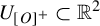 of the half-line
$\Gamma ^{^+}_{[{O}]^+}$
 . Therefore, for any indexing
$[{O}]^+ = \{{O}_{ 1}, \ldots , {O}_{ r}\}$
 , there exists a family
$\{\Gamma ^{^+}_{{O}}\}_{{O} \in [{O}]^+}$
 of pairwise disjoint half-lines
$\Gamma ^{^+}_{{O}} : [0, \infty ) \longrightarrow \mathbb R^2$
 , each positively transverse to
${\mathcal {F}}$
 , such that:
-
• the half-line $\Gamma ^{^+}_{{O}}$
is contained in
$ U_{[{O}]^+}$
for all
${O} \in [{O}]^+$
; -
• the endpoint $\Gamma ^{^+}_{{O}}(0)$
lies on the leaf
$ \phi $
for all
${O} \in [{O}]^+$
; -
• the forward orbit $\overline {L(\phi )} \cap {O} $
is contained in
$\Gamma ^{^+}_{O}$
for all
${O} \in [{O}]^+;$
-
• the endpoints $\{\Gamma ^{^+}_{{O}}(0)\}_{{O} \in [{O}]^+}$
are ordered along the leaf
$\phi $
according to
$\leq $
.


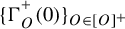


Proof. Using the Homma–Schoenflies theorem, we can assume that:
-
• $\Gamma ^{^+}_{[{O}]^+}([0,\infty ){ }) = [0,\infty ) \times \{0\}$
, oriented positively in the first coordinate; -
• $\phi = \{0\} \times \mathbb R$
, oriented downwards; -
• $[0,\infty )\times [-1,1] \subset U_{[{O}]^+}$
is vertically foliated by
${\mathcal {F}}$
.




Consider an arbitrary enumeration
$[{O}]^+ = \{{O}_{ 1},\ldots ,{O}_{ r}\}$
 . For any
${O}_{ i}, {O}_{ j} \in [{O}]^+$
 , we have
$\partial _L C_{{O}_{ i}} = \partial _L C_{{O}_{ j}}$
 . We denoted this set by
$\partial _L C_{[{O}]^+}.$
 Now, since the closed set
$[0,\infty )\times [-1,1]$
 is trivially foliated by
${\mathcal {F}}$
 and contains the transverse half-line
$\Gamma ^{^+}_{[{O}]^+}$
 , we get that
$[0,\infty )\times [-1,1]$
 is disjoint from
$\partial _L C_{[{O}]^+}$
 . By Lemma 2.2, there exists a family
$\{V_\phi \}_{\phi \in \partial _L C_{[{O}]^+}}$
 of sufficiently small trivial neighborhoods for the leaves in
$\partial _L C_{[{O}]^+}$
 such that each
$V_\phi $
 is disjoint from
$ [0,\infty )\times [-1,1] $
 .
Since each leaf of
${\mathcal {F}}$
 intersects
$\bigcup _{i=1}^r {O}_i$
 at most once, by moving the points of each orbit
${O}_{ i} \in [{O}]^+ $
 vertically, we obtain a homeomorphism
$\varphi: [0,\infty)\times [-1,1] \longrightarrow [0,\infty)\times [-1,1]$
 that fixes each vertical and satisfies
$\varphi ({O}_{ i} \cap \overline {L(\phi )}) \subset [0,\infty )\times \{1/i\}$
 for all
$ i\in \{1,\ldots ,r\}.$
 For each
$i \in \{1,\ldots ,n\}$
 , consider the path
$\Gamma ^+_{i}:[0,\infty ) \longrightarrow \mathbb R^2$
 defined by
$\Gamma ^+_{i}(t) = ( t, 1/i ).$

Observe that each path
$\varphi ^{-1}\circ \Gamma ^+_{i}$
 is positively transverse to
${\mathcal {F}}$
 and disjoint from all trivial neighborhoods in
$\{V_\phi \}_{\phi \in \partial _L C_{[{O}]^+}}$
 . As in the proof of Theorem A, this is enough to imply that each
$\varphi ^{-1}\circ \Gamma ^+_{i}$
 is a half-line.
Therefore, we end up with a family
$\{\varphi ^{-1} \circ \Gamma ^+_i\}_{i=1}^r$
 of pairwise disjoint half-lines positively transverse to
${\mathcal {F}}$
 , contained in
$U_{[{O}]^+}$
 , with their endpoints
$\{\varphi ^{-1} \circ \Gamma ^+_i(0)\}_{i=1}^r$
 ordered increasingly along the leaf
$\phi $
 , i.e.
$\varphi^{-1} \circ \Gamma^+_i(0) < \varphi^{-1} \circ \Gamma^+_{i+1}(0)$
 according to the orientation of
$\phi$
 for all
$i \in \{1, \ldots, r-1\}$
 .
This concludes the proof of the lemma.
7.2 Proof of Theorem B
Proof. Before we start, we pay attention to the fact that the enumeration
${\mathcal {O}} = \{{O}_{ 1},\ldots ,{O}_{ r}\}$
 fixed in the statement of the proposition satisfies
${O}_{ i} \lesssim _L {O}_{ i+1}$
 for all
$i \in \{1, \ldots , r-1\}$
 . This implies that each class
$[{O}]^+ \in {\mathcal {O}}/{\stackrel {+}{\sim }}$
 is associated to an interval of
$\{1,\ldots ,r\}$
 given by

Moreover, the intervals in
$\{I_{[{O}]^+}\}_{[{O}]^+ \in {\mathcal {O}}/{\stackrel {+}{\sim }}}$
 are pairwise disjoint and their arrangement inside the set
$\{1, \ldots , r\}$
 is determined by the total order
$\lesssim _L$
 on
${\mathcal {O}}/{\stackrel {+}{\sim }}$
 .
By applying Lemma 7.3 to the leaf
$\phi $
 and the set of orbits
${\mathcal {O}}$
 , we obtain a family of pairwise disjoint half-lines
$\{\Gamma ^{^+}_{[{O}]^+}\}_{[{O}]^+ \in {\mathcal {O}}/{\stackrel {+}{\sim }}}$
 , each positively transverse to
${\mathcal {F}}$
 and satisfying:
-
• the endpoints $\Gamma ^{^+}_{[{O}]^+}(0)$
lie on the leaf
$\phi $
; -
• the forward orbit $\overline {L(\phi )} \cap {O}_{ i} $
is contained in
$\Gamma ^{^+}_{[{O}]^+}$
for all
$i \in I_{[{O}]^+}$
; -
• for any two distinct classes $[{O}]^+, [{O}']^+ \in {\mathcal {O}}/{\stackrel {+}{\sim }}$
satisfying
$[{O}]^+ \lesssim _L [{O}']^+$
, we have $$ \begin{align*}\Gamma^{^+}_{[{O}]^+}(0) < \Gamma^{^+}_{[{O}']^+}(0) \quad \text{along the leaf } \phi .\end{align*} $$


Next, consider a family
$\{ U_{[{O}]^+}\}_{[{O}]^+ \in {\mathcal {O}}/{\stackrel {+}{\sim }}}$
 of pairwise disjoint open sets satisfying

Finally, for each class
$[{O}]^+ \in {\mathcal {O}}/{\stackrel {+}{\sim }}$
 , we apply Lemma 7.4 to the half-line
$\Gamma ^{^+}_{[{O}]^+}$
 and the open neighborhood
$U_{[{O}]^+}$
 , with respect to the enumeration
$[{O}]^+ = \{{O}_{ i}\}_{i \in I_{[{O}]^+}}$
 . This yields a family of pairwise disjoint half-lines
$\{\Gamma ^{^+}_{ i}\}_{i \in I_{[{O}]^+}}$
 , each positively transverse to
${\mathcal {F}}$
 and satisfying:
-
• the half-line $\Gamma ^{^+}_{ i}$
is contained in the open neighborhood
$U_{[{O}]^+}$
; -
• the forward orbit $\overline {L(\phi )} \cap {O}_{ i} $
is contained in
$\Gamma ^{^+}_{ i}$
; -
• the endpoint $\Gamma ^{^+}_{ i}(0)$
lies on the leaf
$\phi $
; -
• The points $\{\Gamma ^{^+}_{ i}(0)\}_{i \in I_{[{O}]^+}}$
are ordered
$\Gamma ^{^+}_{ i}(0) < \Gamma ^{^+}_{ i+1}(0)$
along the leaf
$\phi $
.


By repeating this process for each class
$[{O}]^+ \in {\mathcal {O}}/{\stackrel {+}{\sim }}$
 , we obtain a family of pairwise disjoint half-lines
$\{\Gamma ^{^+}_{ i}\}_{1\leq i \leq r}$
 that satisfies the conditions stated in the theorem.
By combining Remark 4.6 with Theorem B, we obtain directly the following corollary, which provides an alternative definition of
$\lesssim _L$
 and
$\lesssim _R$
 in terms of proper transverse trajectories (under generic conditions on
$\mathcal{F}$
 ). This result is stated below.
Corollary 7.5. Let
${\mathcal {O}} \subset \mathrm {Orb}(f)$
 be a finite set of orbits and assume that
${\mathcal {F}}$
 is generic for
${\mathcal {O}}$
 . Let
$\phi \in {\mathcal {F}}$
 be a leaf and let
${O},{O}^{\prime } \in {\mathcal {O}}(\phi )$
 be two distinct orbits. Then, we have that
${O}\lesssim _L {O}^{\prime }$
 if, and only if, there exists proper transverse trajectories
$\Gamma _{O}$
 and
$\Gamma _{{O}^{\prime }}$
 of the orbits
${O}$
 and
${O}^{\prime }$
 , respectively, such that the following conditions hold:
-
(i) the trajectories $\Gamma _{O}$
and
$\Gamma _{{O}^{\prime }}$
are disjoint on the left side of
$\phi $
, i.e.
$\Gamma_{O} \cap \Gamma_{{O}^{\prime}} \cap \overline{L(\phi)} = \varnothing$
; -
(ii) the intersection points $p_{O} \in \Gamma _{O} \cap \phi $
and
$p_{{O}^{\prime }} \in \Gamma _{{O}^{\prime }} \cap \phi $
are ordered as
$p_{O} < p_{{O}^{\prime}}$
according to the orientation along the leaf
$\phi$
.







We obtain an analogous result for
$\lesssim _R$
 by replacing each L with R in the above statement.
Moreover, under generic conditions on
${\mathcal {F}}$
 , we also have the following corollary.
Corollary 7.6. Distinct orbits
${O},{O}^{\prime } \in {\mathcal {O}}$
 have a weak
${\mathcal {F}}$
 -transverse intersection if, and only if, every pair of proper transverse trajectories
$\Gamma _{O}$
 and
$\Gamma _{{O}^{\prime }}$
 of
${O}$
 and
${O}^{\prime }$
 intersect.
Proof. It suffices to show that any
${O},{O}^{\prime } \in {\mathcal {O}}$
 not having a weak
${\mathcal {F}}$
 -transverse intersection must admit disjoint proper transverse trajectories. If
$C_{O} \cap C_{{O}^{\prime }} = \varnothing $
 , this result is trivial. Assume that
$C_{O} \cap C_{{O}^{\prime }} \neq \varnothing $
 and consider a leaf
$\phi \in C_{O} \cap C_{{O}^{\prime }}$
 that is disjoint from
${O}$
 and
${O}^{\prime }$
 . Now, consider
$\phi _L, \phi _R \in C_{O} \cap C_{{O}^{\prime }}$
 with
$L(\phi _L) \subset L(\phi _R)$
 sufficiently close to
$\phi $
 so that the set
$ \overline {L(\phi _R) \cap R(\phi _L)}$
 is disjoint from
${O}$
 and
${O}^{\prime }$
 . By Corollary 7.5, we get proper transverse trajectories
$\Gamma _{O}$
 and
$\Gamma _{{O}^{\prime }}$
 for
${O}$
 and
${O}^{\prime }$
 that are disjoint on
$L(\phi_L)\cup R(\phi_R)$
 . Since
${O}$
 and
${O}^{\prime }$
 do not have a weak
${\mathcal {F}}$
 -transverse intersection,
$\Gamma _{O}$
 and
$\Gamma _{{O}^{\prime }}$
 can be taken to intersect the leaves
$\phi _L$
 and
$\phi _R$
 in the same order. Thus, we can easily modify
$\Gamma _{O}$
 and
$\Gamma _{{O}^{\prime }}$
 inside
$\overline {L(\phi _R) \cap R(\phi _L)}$
 so that they become disjoint, while preserving the properties of being proper.
8 Adaptive orders across maximal leaf domains
We begin this section with an illustrative scenario that motivates Theorem C (Figure 43).
Let
${\mathcal {O}}\subset \mathrm {Orb}(f)$
 be a finite collection of orbits and let
${\mathcal {D}}_{\mathcal {O}}$
 be the decomposition by maximal leaf domains induced by
${\mathcal {O}}$
 . Consider a maximal leaf domain
$D\in {\mathcal {D}}_{O}$
 and a pair of sufficiently close leaves
$\phi _L, \phi _R \in D$
 satisfying
$L(\phi _L) \subset L(\phi _R)$
 . Now, assume that there exists a family of proper transverse trajectories
$\{\Gamma _{O}\}_{{O} \in {\mathcal {O}}(D)}$
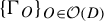 for
${\mathcal {O}}(D)$
 such that

Illustrative scenario that explains the idea behind the proof of Theorem C.

Figure 43 Long description
A two-panel vector field diagram separated by a narrow vertical gap. At the top of the gap, the left axis is labeled phi sub R and the right axis is labeled phi sub L. Both axes have downward-pointing arrows.
On the left side, numerous gray and black streamlines flow from the far left toward the central axis. A blue line labeled Gamma sub O and a red line labeled Gamma sub O prime are highlighted among the black lines. These lines curve inward as they approach the phi sub R axis.
On the right side, the flow mirrors the left, moving from the phi sub L axis outward to the right. The blue line Gamma sub O and red line Gamma sub O prime continue here. In the middle of the right panel, these two lines cross each other in an X-shaped intersection before continuing horizontally. A similar X-shaped crossing occurs between two black streamlines lower down in the right panel. The background is filled with lighter gray contour lines that follow the general flow of the darker black and colored trajectories.
We want such a family
$\{\Gamma _{O}\}_{{O} \in {\mathcal {O}}(D)}$
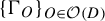 to follow the following principles.
-
• If two orbits ${O},{O}^{\prime } \in {\mathcal {O}}(D)$
have a weak
${\mathcal {F}}$
-transverse intersection, we ask ourselves $$ \begin{align*}\text{`Does there exist some } D^{\prime} \in {\mathcal{D}}_{\mathcal{O}} \text{ satisfying } D \leadsto D^{\prime} \text{ for which } {O},{O}^{\prime} \in {\mathcal{O}}(D^{\prime})?'\end{align*} $$If the answer is ‘YES’, then we want the trajectories $\Gamma _{O}$
and
$\Gamma _{{O}^{\prime }}$
to be disjoint inside D, leaving their obligatory intersection to happen in
$D^ {\prime }$
, or later if possible.
If the answer is ‘NO’, then we want the obligatory intersection between $\Gamma _{O}$
and
$\Gamma _{{O}^{\prime }}$
to happen in a single point inside D, specifically, in between the leaves
$\phi _L$
and
$\phi _R$
; -
• If two orbits ${O},{O}^{\prime } \in {\mathcal {O}}(D)$
do not have a weak
${\mathcal {F}}$
-transverse intersection, then we simply want the trajectories
$\Gamma _{O}$
and
$\Gamma _{{O}^{\prime }}$
to be disjoint.



Observe that any family
$\{\Gamma _{O}\}_{{O} \in {\mathcal {O}}(D)}$
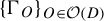 as described above would prove Theorem C in the particular case where
${\mathcal {O}} = {\mathcal {O}}(D)$
 . Therefore, to prove Theorem C in the general case, we not only need to construct such a family
$\{\Gamma _{O}\}_{{O} \in {\mathcal {O}}(D)}$
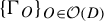 for each
$D \in {\mathcal {D}}_{\mathcal {O}}$
 , but also to do so in a coherent way, so that the resulting family
$\{\Gamma _{O}\}_{{O} \in {\mathcal {O}}}$
 solves the theorem.
This problem is solved by defining a ‘standard’ total order
$\leq _\phi $
 on the set
${\mathcal {O}}(\phi )$
 of orbits crossing a leaf
$\phi \in {\mathcal {F}}$
 , and an ‘adaptive’ total order
$\leq _{D}$
 on the set
${\mathcal {O}}(D)$
 of orbits crossing a maximal leaf domain
$D \in {\mathcal {D}}_{\mathcal {O}}$
 .
Now, we come back to the general setting. Let
${\mathcal {O}}\subset \mathrm {Orb}(f)$
 be a finite collection of orbits and let
${\mathcal {D}}_{\mathcal {O}}$
 be the decomposition by maximal leaf domains induced by
${\mathcal {O}}$
 . Before we proceed with the definitions of the standard and adaptive orders, we chose to denote the equivalence relation of backward and forward
${\mathcal {F}}$
 -asymptotic orbits in
${\mathcal {O}}$
 by
$\sim $
 , that is,

Then, we fix an arbitrary total order
$\leq _{[{O}]}$
 on each equivalence class
$[{O}] \in {\mathcal {O}}/\sim $
 . This choice of total orders
$\{\leq _{[{O}]}\}_{[{O}] \in {\mathcal {O}}/\sim }$
 determine the standard and adaptive orders defined below.
8.0.1 Standard ordering over leaves
For each leaf
$\phi \in {\mathcal {F}}$
 , we consider the relation
$\leq _\phi $
 on the set
${\mathcal {O}}(\phi )$
 , defined as follows:

Roughly speaking, the relation
$\leq _\phi $
 primarily compares orbits in
${\mathcal {O}}(\phi )$
 using the relation
$\lesssim _R$
 . If the compared orbits are backward
${\mathcal {F}}$
 -asymptotic, then it tries to compare them using the relation
$\lesssim _L$
 . At last, if the orbits are both forward and backward
${\mathcal {F}}$
 -asymptotic, then it uses the total order
$\leq _{[{O}]}$
 defined on the equivalence class
$[{O}] \in {\mathcal {O}}/{\sim }$
 of these orbits.
Lemma 8.1. For any leaf
$\phi \in {\mathcal {F}}$
 , the relation
$\leq _\phi $
 is a total order on the set
${\mathcal {O}}(\phi )$
 .
Proof. Let
$\phi \in {\mathcal {F}}$
 be a leaf and recall that
$\lesssim _R$
 induces a total order on the set
${\mathcal {O}}(\phi )/{\stackrel {-}{\sim }}$
 . Thus, we can enumerate the set
${\mathcal {O}}(\phi )/{\stackrel {-}{\sim }}$
 increasingly with respect to
$\lesssim _R$
 , that is,

Then, for each
$i \in \{1, \ldots , r\}$
 , since
$\lesssim _L$
 induces a total order on the set
${\mathcal {O}}_{ i}/{\stackrel {+}{\sim }}$
 , we can enumerate it increasingly with respect to
$\lesssim _L$
 , that is,

At last, note that, for any
$i \in \{1, \ldots , r\}$
 and
$j \in \{1, \ldots , m(i)\}$
 , it holds that
${\mathcal {O}}_{ i,j} \in {\mathcal {O}}(\phi )/{\sim }$
 . Thus, there exists an equivalence class
$[{O}]_{ i,j} \in {\mathcal {O}}/{\sim }$
 such that
${\mathcal {O}}_{ i,j} \subset [{O}]_{ i,j}$
 . We can enumerate
${\mathcal {O}}_{ i,j}$
 increasingly with respect to the initially fixed total order
$\leq _{[{O}]_{ i,j}}$
 , that is,

At the end, we obtained a triple index enumeration of the set
${\mathcal {O}}(\phi )=\{{O}_{ i,j,k}\}_{i,j,k}$
 , where the indices run through
$i \in \{1, \ldots , r\}$
 ,
$j \in \{1, \ldots , m(i)\}$
 and
$k \in \{1, \ldots , n(i,j)\}$
 .
By construction,
$\leq _\phi $
 coincides with the lexicographic order on
${\mathcal {O}}(\phi )=\{{O}_{ i,j,k}\}_{i,j,k}$
 , i.e.

This proves that
$\leq _\phi $
 is a total order on the set
${\mathcal {O}}(\phi )$
 and concludes the proof.
8.1 Adaptive ordering over maximal leaf domains
For each
$D \in {\mathcal {D}}_{{\mathcal {O}}}$
 , we consider an equivalence relation
$\stackrel {D}{\sim }$
 on the set
${\mathcal {O}}(D)$
 that is slightly weaker than the relation
$\stackrel {+}{\sim }$
 .
For any two orbits
${O},{O}^{\prime } \in {\mathcal {O}}(D)$
 , we say that
${O} \stackrel {D}{\sim } {O}^{\prime }$
 if:
-
• either ${O},{O}^{\prime }\in {\mathcal {O}}_\omega (D)$
and they satisfy
${O} \stackrel {+}{\sim } {O}^{\prime }$
; -
• or ${O},{O}^{\prime } \in {\mathcal {O}}_{\mathrm {out}}(D)$
and there exists a leaf
$\phi _L \in \partial _L D$
such that
${O}, {O}^{\prime } \in {\mathcal {O}}(\phi _L)$
.


We observe that if the orbits
${O}$
 and
${O}^{\prime }$
 satisfy
${O}\stackrel {+}{\sim } {O}^{\prime }$
 , then they must also satisfy
${O} \stackrel {D}{\sim } {O}^{\prime }$
 , but the converse does not hold in general, only if the orbits
${O}$
 and
${O}^{\prime }$
 are both in
${\mathcal {O}}_\omega (D)$
 . Moreover, note that the relation
$\lesssim _L$
 induces a total order on the set
${\mathcal {O}}(D)/{\stackrel {D}{\sim }}$
 . This follows from the fact that if the orbits
${O},{O}^{\prime },{O}^{ \prime \prime } \in {\mathcal {O}}_{\mathrm {out}}(D)$
 satisfy
${O} \lesssim _L {O}^{\prime } \lesssim _L {O}^{ \prime \prime }$
 and
${O} \stackrel {D}{\sim } {O}^{ \prime \prime }$
 , then they must also satisfy
${O}\stackrel {D}{\sim } {O}^{ \prime \prime }$
 .
With this equivalence relation, we can define the relation
$\leq _D$
 on the set
${\mathcal {O}}(D)$
 as follows:

Roughly speaking,
$\leq _D$
 primarily compares orbits in
${\mathcal {O}}(D)$
 using the relation
$\lesssim _L$
 . If the compared orbits exit the domain D through the same leaf
$ \phi _L \in \partial _L D$
 , then it tries to compare them using
$\lesssim _R$
 . At last, if these orbits are both forward and backward
${\mathcal {F}}$
 -asymptotic, then it uses the total order
$\leq _{[{O}]}$
 on their equivalence class
$[{O}] \in {\mathcal {O}}/{\sim }$
 to compare them.
Note that
$\leq _D$
 may be viewed as an analog of
$\leq _\phi $
 , with the roles of
$\lesssim _L$
 and
$\lesssim _R$
 essentially reversed, except in the case where the compared orbits exit D through the same leaf in
$\partial _L D$
 , in which case, the relation
$\lesssim _R$
 continues to be applied.
Lemma 8.2. For any
$D \in {\mathcal {D}}_{\mathcal {O}}$
 , the relation
$\leq _D$
 is a total order on the set
${\mathcal {O}}(D)$
 .
Proof. The proof is completely analogous to the proof of Lemma 8.1.
9 Proof of Theorem C
This section is dedicated to the proof of Theorem C. The version of the theorem stated here is slightly different from the one presented in the introduction (see Remark 9.1).
Theorem C. Let
${\mathcal {O}}\subset \mathrm {Orb}(f)$
 be a finite collection of orbits. Assume
${\mathcal {F}}$
 is generic for
${\mathcal {O}}$
 . Then, there exists a family
$\{\Gamma _{O}\}_{{O} \in {\mathcal {O}}}$
 of proper transverse trajectories of
${\mathcal {O}}$
 that satisfies:
-
(i) $\#( \Gamma _{O} \cap \Gamma _{{O}^{\prime }} ) \leq 1$
for any pair of distinct orbits
${O},{O}^{\prime } \in {\mathcal {O}}$
; -
(ii) $\#( \Gamma _{O} \cap \Gamma _{{O}^{\prime }} ) = 1$
if, and only if,
${O}$
and
${O}^{\prime }$
have a weak
${\mathcal {F}}$
-transverse intersection.


Remark 9.1. The version of Theorem C enunciated in the introduction is a direct consequence of the statement above combined with the following argument. We enumerate
${\mathcal {O}} = \{{O}_{ 1}, \ldots , {O}_{ r}\}$
 and consider the family of proper transverse trajectories
$\{\Gamma _{i}\}_{1\leq i \leq r}$
 given by Theorem C. Then, consider a collection of planar foliations
$\{{\mathcal {F}}_j\}_{1\leq j \leq n}$
 which are pairwise transverse to each other, and such that
${\mathcal {F}}_0 = {\mathcal {F}}$
 and for each
$1\leq i \leq r$
 , there exists
$1\leq j \leq n$
 such that
$\Gamma _i \in {\mathcal {F}}_j$
 . The homeomorphism
$\varphi :\mathbb R^2 \longrightarrow \mathbb D^2$
 in the statement of Theorem C in the introduction is given by the circle compactification of
$\mathbb R^2$
 via ideal boundaries of
$\{{\mathcal {F}}_j\}_{1\leq j \leq n}$
 , as described in [Reference BonattiBon24].
Proof. Let
${\mathcal {D}}_{{\mathcal {O}}}$
 be the decomposition into the maximal leaf domain induced by
${\mathcal {O}}$
 and let
$\mathcal W_{{\mathcal {O}}}$
 be the set of critical leaves for
${\mathcal {O}}$
 (see §6). Next, fix an arbitrary total order
$\leq _{[{O}]}$
 on each equivalence class
$[{O}] \in {\mathcal {O}}/{\sim }$
 , where
$\sim $
 consists in the equivalence relation of backward and forward
${\mathcal {F}}$
 -asymptotic orbits in
${\mathcal {O}}$
 . As explained in §8, this choice of total orders
$\{\leq _{[{O}]}\}_{[{O}] \in {\mathcal {O}}/\sim }$
 determines the standard order
$\leq _\phi $
 and the adaptive order
$\leq _D$
 , which are total orders on
${\mathcal {O}}(\phi )$
 and
${\mathcal {O}}(D)$
 , respectively, for each
$\phi \in {\mathcal {F}}$
 and each
${D \in {\mathcal {D}}_{{\mathcal {O}}}}$
 .
For each leaf
$\phi \in \mathcal W_{{\mathcal {O}}}$
 , we consider a family of pairwise distinct points
$\{p_{\phi }({O})\}_{{O} \in {\mathcal {O}}(\phi )}$
 lying on the leaf
$\phi $
 , such that the points
$p_{\phi }({O})$
 are ordered along
$\phi $
 according to
$\leq _\phi $
 , that is,

In the case where the leaf
$\phi \in \mathcal W_{{\mathcal {O}}}$
 intersects some orbit
${O} \in {\mathcal {O}}(\phi )$
 , then we can choose the point
$p_{\phi }({O})$
 to be exactly the intersection point
$\phi \cap {O} = \{p_{\phi }({O})\}$
 .
Fix a leaf domain
$D \in {\mathcal {D}}_{{\mathcal {O}}}$
 and let
$\phi _L, \phi _R \in D$
 be two leaves with
$ L(\phi _L) \subset L(\phi _R)$
 that are sufficiently close and sufficiently to the left so that they satisfy

Now, consider a family of pairwise distinct points
$\{q_{_{R,D}}({O})\}_{{O} \in {\mathcal {O}}(D)}$
 lying on the leaf
$\phi _R$
 and ordered according to the standard total order
$\leq _{\phi _R}$
 on the set
${\mathcal {O}}(D) = {\mathcal {O}}(\phi _R)$
 .
Observe that the order
$\leq _{\phi _R}$
 allows us to apply the right-analogous version of Theorem B to the leaf
$\phi _R$
 and to the set orbits
${\mathcal {O}}(D)$
 indexed increasingly by
$\leq _{\phi _R}$
 ; thus, obtaining a family of pairwise disjoint half-lines
$\{\Gamma ^{^-}_{D, {O}}\}_{{O} \in {\mathcal {O}}(D)}$
 , each positively transverse to
${\mathcal {F}}$
 , that satisfies:
-
• the endpoint $\Gamma ^{^-}_{D, {O}}(0)$
lies on the leaf
$ \phi _R$
for all
${O} \in {\mathcal {O}}(D)$
; -
• the backward orbit $\overline {R(\phi _R)} \cap {O} $
is contained in
$\Gamma ^{^-}_{D, {O}}$
for all
${O} \in {\mathcal {O}}(D)$
; -
• the endpoints $\{\Gamma ^{^-}_{D, {O}}(0)\}_{{O} \in {\mathcal {O}}(D)}$
are ordered along the leaf
$\phi _R$
according to
$\leq _{\phi _R}$
.


We remark that the proof of Theorem B gives us enough flexibility to choose the half-lines in the family
$\{\Gamma ^{^-}_{D, {O}}\}_{{O} \in {\mathcal {O}}(D)}$
 so that they satisfy the following additional properties:
-
• $\Gamma ^{^-}_{D, {O}}(0) = q_{_{R,D}}({O})$
for any
${O} \in {\mathcal {O}}(D)$
; -
• $p_{\phi ^{\prime }}({O}) \in \Gamma ^{^-}_{D, {O}}$
for any
${O} \in {\mathcal {O}}_{\mathrm {in}}(D)$
, where
$\phi ^{\prime }$
denotes the unique leaf in
$\partial _R D \cap C_{O}$
.


At last, for each orbit
${O} \in {\mathcal {O}}_{\mathrm {in}}(D)$
 , we cut
$\Gamma ^{^-}_{D, {O}}$
 at its intersection point with
$\partial _R D$
 so that it stays inside D and it joins
$\partial _R D$
 to
$\phi _R$
 . In other words, we redefine
$\Gamma ^{^-}_{D, {O}}:[0,1]\longrightarrow \mathbb R^2$
 as the sub-arc of the originally defined half-line
$\Gamma ^{^-}_{D, {O}}$
 that ends at the point
$q_{_{R,D}}({O}) \in \phi _R$
 and starts at the point
$p_{\phi ^{\prime }}({O}) \in \phi ^{\prime }$
 , where
$\phi ^{\prime }$
 is the unique leaf in
$\partial _R D \cap C_{O}$
 .
Now, consider a family of pairwise distinct points
$\{q_{_{L,D}}({O})\}_{{O} \in {\mathcal {O}}(D)}$
 lying on
$\phi _L$
 and ordered increasingly along
$\phi_L$
 according to the adaptive total order
$\leq _{D}$
 .
Observe that the order
$\leq _{D}$
 only allows us to apply Theorem B to the leaf
$\phi _L$
 and the subset
${\mathcal {O}}_\omega (D) \subset {\mathcal {O}}(D)$
 indexed increasingly by
$\leq _{D}$
 , as the order
$\leq _{D}$
 is not necessarily compatible with
$\lesssim _L$
 on orbits leaving D through the same leaf in
$\partial _L D$
 . However, this is enough to obtain (see Figure 44) a family of pairwise disjoint half-lines
$\{\Gamma ^{^+}_{D, {O}}\}_{{O} \in {\mathcal {O}}_\omega (D)}$
 positively transverse to
${\mathcal {F}}$
 such that:
-
• the endpoint $\Gamma ^{^+}_{D, {O}}(0)$
coincides with the point
$q_{_{L,D}}({O})\in \phi _L$
for all
${O} \in {\mathcal {O}}_\omega (D)$
; -
• the forward orbit $\overline {L(\phi _L)} \cap {O} $
is contained in
$\Gamma ^{^+}_{D, {O}}$
for all
${O} \in {\mathcal {O}}_\omega (D).$


Families
$\{\Gamma^{^-}_{D, O}\}_{O \in \mathcal{O}(D)} $
 and
$\{\Gamma^{^+}_{D, O}\}_{O \in \mathcal{O}_\omega(D)}$
 constructed in the proof of Theorem C.

Figure 44 Long description
A vector field plot is divided into two main regions by a central vertical wavy boundary.
On the left side, a family of blue streamlines, labeled as Gamma super minus sub D comma O where O is in mathcal O of D, flows from left to right. These lines are mostly horizontal but converge slightly as they approach the boundary.
The boundary consists of two parallel wavy black lines labeled phi sub R and phi sub L at the top.
On the right side, a family of red streamlines, labeled as Gamma super plus sub D comma O where O is in mathcal O sub omega of D, originates from the boundary and flows to the right. These red lines weave between three horizontal U-shaped black curves that open to the right. Inside these U-shaped regions are horizontal rows of red dots.
Faint gray background streamlines show a complex underlying flow pattern with several vortices and saddle points throughout the entire domain.
Observe that for each orbit
${O} \in {\mathcal {O}}_{\mathrm {out}}(D)$
 , we have a leaf
$\phi ^{\prime } \in \partial _L D$
 such that
${{O} \in {\mathcal {O}}(\phi ^{\prime })}$
 and we can construct a path
$\Gamma _{D,{O}}^{^+}:[-1,0]\longrightarrow \mathbb R^2$
 positively transverse to
${\mathcal {F}}$
 that connects the point
$q_{_{L,D}}({O})\in \phi _L$
 to the point
$p_{\phi ^{\prime }}({O}) \in \phi ^{\prime }$
 . By constructing these paths one at a time, we can construct them so that the family
$\{\Gamma _{D,{O}}^{^+}\}_{{O} \in {\mathcal {O}}_{\mathrm {out}}(D)}$
 is pairwise disjoint and, moreover, so that they are each disjoint from the already constructed
$\{\Gamma ^{^-}_{D, {O}}\}_{{O} \in {\mathcal {O}}_\omega (D)}$
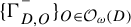 .
To summarize, we have two families
$\{\Gamma ^{^-}_{D, {O}}\}_{{O} \in {\mathcal {O}}(D)}$
 and
$\{\Gamma ^{^+}_{D, {O}}\}_{{O} \in {\mathcal {O}}(D)}$
 formed by pairwise disjoint half-lines positively transverse to
${\mathcal {F}}$
 such that, for each
${O} \in {\mathcal {O}}(D)$
 , the following properties hold:

Now, using the Homma–Schoenflies theorem, we can assume up to conjugacy that:
-
• the leaves $ \phi _R $
and
$ \phi _L $
are vertical, with
$ \phi _R = \{0\} \times \mathbb {R} $
and
$ \phi _L = \{1\} \times \mathbb {R} $
; -
• the square $ [0,1] \times [0,1] $
is foliated vertically by
$ \mathcal {F} $
; -
• the endpoints $ \{q_{_{R,D}}({O})\}_{{O} \in {\mathcal {O}}(D)} $
lie on the side of the square
$ \{0\} \times [0,1] $
; -
• the endpoints $ \{q_{_{L,D}}({O})\}_{{O} \in {\mathcal {O}}(D)} $
lie on the side of the square
$ \{1\} \times [0,1] $
.


For each
$ {O} \in {\mathcal {O}}(D) $
 , let
$ \gamma _{_{D,{O}}}:[0,1] \longrightarrow \mathbb {R}^2 $
 be the line segment joining
$ q_{_{R,D}}({O}) $
 to
$ q_{_{L,D}}({O}) $
 . Observe that, from the definition of the standard order
$\leq _{\phi _R}$
 and the adaptive order
$\leq _D$
 , the segments in the family
$ \{\gamma _{_{D,{O}}}\}_{{O} \in {\mathcal {O}}(D)} $
 satisfy the following properties:
-
• $ \#(\gamma _{_{D,{O}}} \cap \gamma _{_{D,{O}^{\prime }}}) = 1 $
if and only if the orbits
$ {O} $
and
$ {O}^{ \prime } $
have a weak
${\mathcal {F}}$
-transverse intersection, and there exists no
$ D' \in {\mathcal {D}}_{{\mathcal {O}}} $
such that
$ D \leadsto D' $
and
$ {O}, {O}^{ \prime } \in {\mathcal {O}}(D') $
; -
• $ \#(\gamma _{_{D,{O}}} \cap \gamma _{_{D,{O}^{\prime }}}) = 0 $
otherwise.


For each orbit
$ {O} \in {\mathcal {O}}(D) $
 , we define the concatenated path
$\Gamma_{D,{O}} := \Gamma^{^-}_{D, {O}} \cup \gamma_{_{D,{O}}} \cup \Gamma^{^+}_{D, {O}}$
 .
To conclude, we repeat the construction for each maximal leaf domain
${ D \in {\mathcal {D}}_{{\mathcal {O}}} }$
 . Then, we recall that for any orbit
$ {O} \in {\mathcal {O}}(D) $
 , we have a sequence of maximal leaf domains

such that
${O}$
 belongs to the sets
${\mathcal {O}}_\alpha (D_0)$
 and
${\mathcal {O}}_\omega (D_{m_{O}})$
 . Then, this allows us to construct a proper transverse trajectory of the orbit
$ {O} $
 as the concatenation of the paths

The resulting family of proper transverse trajectories
$ \{\Gamma _{O}\}_{{O} \in {\mathcal {O}}} $
 proves the theorem.
Acknowledgements
This project has received funding from the European Union’s Horizon 2020 research and innovation program under the Marie Skłodowska-Curie grant agreement No. 945332  .