

1. Introduction
There has been significant recent interest in the problem of counting elliptic curves of bounded height over the rational numbers
 $\mathbb{Q}$
, or more generally over a fixed number field K, which have a prescribed torsion group structure. Works following this trend [
Reference Boggess and Sankar3, Reference Bruin and Najman5, Reference Cullinan, Kenney and Voight7, Reference Harron and Snowden11, Reference Molnar and Voight20, Reference Phillips24, Reference Pizzo, Pomerance and Voight25, Reference Pomerance and Schaefer26
] take the perspective of counting points of bounded height on modular curves parameterising elliptic curves with a specified structure.
In this paper, we count points of bounded height on certain compact Shimura curves of genus zero. Let
 $ {\mathcal X} ^D$
denote the Shimura curve defined over K which parameterises abelian surfaces with fixed quaternionic multiplication (QM) structure by the quaternion algebra over
 $ {\mathbb Q}$
of discriminant D. This curve has genus zero for
 $D\in \{6,10,22\}$
. We count points on the corresponding Shimura curves
 $ {\mathcal X} ^6$
,
 $ {\mathcal X} ^{10}$
, and
 $ {\mathcal X} ^{22}$
, and also on their Atkin–Lehner quotients, which parameterise abelian surfaces with potential quaternionic multiplication (PQM). This is a step towards more generally answering these types of counting problems for abelian varieties of higher dimension, accessed by restricting to a case where extra structure provides a one-dimensional moduli space like for modular curves. We count via the Igusa invariants of corresponding families of genus 2 curves. For
 $D\in \{6,10\}$
these families of curves first appeared in work of Hashimoto–Murabayashi [
Reference Hashimoto and Murabayashi12
] and have also been studied by Baba–Granath [
Reference Baba and Granath2
]. For
 $D=22$
, we use generalisations of these results due to Nualart Riera [
Reference Nualart Riera22
] and Lin–Yang [
Reference Lin and Yang16
].
For
 $D \in \{6,10,22\}$
, let
 $\mathrm{AL}( {\mathcal X} ^D)$
denote the full group of Atkin–Lehner involutions on
 $ {\mathcal X} ^D$
, and let
 $ {\mathcal A} _2$
denote the moduli stack of principally polarised abelian surfaces. For each subgroup
 $W \leq \mathrm{AL}( {\mathcal X} ^D)$
, [
Reference Baba and Granath2
], [
Reference Hashimoto and Murabayashi12
] and [
Reference Nualart Riera22
] describe families
 $C_{W}^D$
of genus 2 curves corresponding to the image of
 $ {\mathcal X} ^D/W$
in
 $ {\mathcal A} _2$
under the map forgetting the QM structure. We discuss these families further in Section 2 and Section 5·2. For any number field K, the Igusa invariants give a map into a weighted projective stack
 \[C^D_{W}(K) \xrightarrow{ {\mathscr I}} {\mathcal P}(1,2,3,5)(\overline{K}).\]
From this map and a height function on the weighted projective stack we define an Igusa height function
 $\overline{\operatorname{Ht}}$
on
 $\overline{K}$
-isomorphism classes of genus two curves. We also define a height
 $\operatorname{Ht}$
on K-isomorphism classes of genus two curves in such a way that results on Malle’s conjecture for counting field extensions can be used to count genus two curves in twist classes.Footnote
1
Let
 $B \in \mathbb{R}_{\gt 0}$
, and let
 $\overline{\mathcal{N}}^{D}(W,K,B)$
(resp.
 $\mathcal{N}^{D}(W,K,B)$
) be the counting function for the number of
 $\overline{K}$
-isomorphism classes (resp. K-isomorphism classes) of curves C in
 $C_{W}^{D}(K)$
with K a field of definition and whose Igusa height
 $\overline{\operatorname{Ht}}(C)$
(resp. whose height
 $\operatorname{Ht}(C)$
) is bounded by B. With this setup, we state our main result.
Theorem 1·1. We have that
 \begin{align*}\overline{\mathcal{N}}^6(W,K,B)\asymp \mathcal{N}^6(W,K,B) &\ll\begin{cases} B^2/\log(B) &\text{ if } W\in\{\langle w_3\rangle, \mathrm{AL}( {\mathcal X} ^6)\}, \\ B^2/\log(B)^{1/2} &\text{ if } W\in\{\langle w_2\rangle, \langle w_6\rangle\},\\ B^2 &\text{ if } W= \{\mathrm{id}\} \text{ and } (\!-6,2)_K=1, \\ 0 &\text{ if } W=\{\mathrm{id}\} \text{ and } (\!-6,2)_K=-1,\end{cases}\\ \overline{\mathcal{N}}^{10}(W,K,B)\ll&\begin{cases} B/\log(B) &\text{ if } W\in\{\langle w_2\rangle, \mathrm{AL}( {\mathcal X} ^{10})\}, \\ B/\log(B)^{1/2} &\text{ if } W\in\{\langle w_5\rangle, \langle w_{10}\rangle\},\\ B &\text{ if } W=\{\mathrm{id}\} \text{ and } (\!-10,5)_K=1, \\ 0 &\text{ if } W=\{\mathrm{id}\} \text{ and } (\!-10,5)_K=-1,\end{cases}\\ \mathcal{N}^{10}(W,K,B)\ll&\begin{cases} B &\text{ if } W\in\{\langle w_2\rangle, \mathrm{AL}( {\mathcal X} ^{10})\}, \\ B\log(B)^{1/2} &\text{ if } W\in\{\langle w_5\rangle, \langle w_{10}\rangle\},\\ B\log(B) &\text{ if } W=\{\mathrm{id}\} \text{ and } (\!-10,5)_K=1, \\ 0 &\text{ if } W=\{\mathrm{id}\} \text{ and } (\!-10,5)_K=-1,\end{cases}\\ \overline{\mathcal{N}}^{22}(W,K,B)\ll&\begin{cases} B^{2/5}/\log(B)^{3/2} &\text{ if } W\in\{\langle w_2\rangle, \mathrm{AL}( {\mathcal X} ^{22})\} \\[3.9pt] &\text{ or if } W=\langle w_{11}\rangle \text{ and } \mathbb{Q}(\sqrt{-11}) \subseteq K,\\[3.9pt] B^{2/5}/\log(B) &\text{ if } W = \langle w_{22}\rangle \\[3.9pt] &\text{ or if } W=\{\mathrm{id}\} \text{ and } \mathbb{Q}(\sqrt{-11}) \subseteq K, \end{cases}\\[3.9pt] \mathcal{N}^{22}(W,K,B)\asymp&\begin{cases} B &\text{ if } W\in\{\langle w_2\rangle, \langle w_{22} \rangle, \mathrm{AL}( {\mathcal X} ^{22})\} \\[3.9pt] &\text{ or if } W\in\{\{\mathrm{id}\}, \langle w_{11}\rangle\} \text{ and } \mathbb{Q}(\sqrt{-11}) \subseteq K. \end{cases}\end{align*}
These bounds are sharp if
 $K=\mathbb{Q}$
or if both
 $D\in\{6,10\}$
and
 $W=\{\mathrm{id}\}$
.
Remark 1·2. The bounds in Theorem 1·1 are expected to be sharp in all cases by a conjecture of Loughran and Smeets [
Reference Loughran and Smeets18
, conjecture 1·6]. The bounds are sharp in the case
 $K=\mathbb{Q}$
, due to a result of Loughran and Matthiesen [
Reference Loughran and Matthiesen17
, corollary 1·2] on counting the number of fibers of a conic bundle over
 $ {\mathbb P}^1$
containing a rational point over
 $\mathbb{Q}$
. Generalising [
Reference Loughran and Matthiesen17
, corollary 1·2] to arbitrary number fields would make the bounds in Theorem 1·1 sharp in all cases.
Remark 1·3. Theorem 1·1 makes no statement about counts if
 $W \in \{\{\mathrm{id}\},\langle w_{11}\rangle\}$
and K does not contain
 $\mathbb{Q}(\sqrt{-11})$
in the
 $D=22$
case. See the proof of Theorem 5·11 for details.
The conditions for having rational points on the top curves
 $ {\mathcal X} ^{6}$
and
 $ {\mathcal X} ^{10}$
(that is, in the
 $W = \{\mathrm{id}\}$
cases) seen above are to be expected; by a result of Shimura [
Reference Shimura32
, theorem 0], the curve
 $ {\mathcal X} ^{D}$
has no real points for
 $D\gt1$
. Furthermore, a result of Jordan [
Reference Jordan14
, theorem 2·1·3] states that an abelian surface with QM by quaternion discriminant D and with no non-trivial automorphisms has a model over a field L containing its field of moduli if and only if L splits the quaternion algebra over
 $\mathbb{Q}$
of discriminant D. The non-trivial quotients of these curves, on the other hand, are not pointless over
 $\mathbb{Q}$
; for
 $D \in \{6,10,22\}$
and for each non-trivial
 $W \leq \mathrm{AL}( {\mathcal X} ^{D})$
, the coarse moduli space
 $X^D/W$
of
 $ {\mathcal X} ^D/W$
is isomorphic to
 $\mathbb{P}^1_{\mathbb{Q}}$
.
A novel feature of our study comes from the fact that a PQM abelian surface need not have a model defined over its field of moduli. This does not occur for elliptic curves, where the field of moduli of an elliptic curve is always a field of definition, as determined by Deligne–Rapoport [ Reference Deligne and Rapoport8 , section VI, proposition 3·2]. The obstruction to a genus 2 curve corresponding to a PQM abelian surface having a model over its field of moduli is explicitly given by Mestre as equivalent to the splitting of a specified conic. This obstruction leads us to consider the problem of counting the number of fibers of certain conic bundles that contain a rational point. To address this, we adapt general counting results of Loughran–Smeets [ Reference Loughran and Smeets18 ] and Loughran–Matthiesen [ Reference Loughran and Matthiesen17 ] (see Proposition 4·1).
Our paper is structured as follows. In Section 2, we give a brief overview of basic facts about Shimura curves and their Atkin–Lehner quotients. In Section 3, we define our height functions, prove an upper bound for counting
 $D_4$
-octic extensions (Proposition 3·4), and prove a result for finding asymptotics for the product of sets (Lemma 3·5). In Section 4, we prove Proposition 4·1 which will allow us to account for the Mestre obstruction in our point counts. The proof of Theorem 1·1 then comes in three parts: Theorem 5·2 and Theorem 5·3 in Section 5·3 for the
 $D=6$
case; Theorem 5·6 and Theorem 5·7 in Section 5·4 for the
 $D=10$
case; and Theorem 5·11 and Theorem 5·12 in Section 5·5 for the
 $D=22$
case.
2. Preliminaries on Shimura curves
2·1. Shimura curves
Let B be a quaternion algebra over
 $\mathbb{Q}$
of discriminant D. Suppose that B is indefinite, meaning that
 $B \otimes_{\mathbb{Q}} \mathbb{R} \cong M_2(\mathbb{R})$
. It follows that
 $D=p_1\cdot p_2\cdots p_{2r}$
is a product of an even number of rational primes, namely those at which B is ramified, and that B is unique up to isomorphism. Let
 $\mathcal{O}$
be a maximal order in B (unique up to conjugacy in
 $B^\times$
).
Let
 $\bar{\ }:\; B\to B$
denote the standard involution on B (i.e., the unique involution for which
 $\overline{b}b\in \mathbb{Q}$
for all
 $b\in B$
). A principal polarisation on B is an element of
 $ {\mathcal O} $
satisfying
 $\mu^2=-D$
. To
 $\mu$
we associate an involution
 \begin{align*} \rho_\mu\;:\; B &\to B\\ b &\mapsto \mu^{-1}\overline{b}\mu,\end{align*}
and further we associate to
 $\mu$
the moduli problem of classifying triples
 $(A,\lambda, \iota)$
, where:
-
(1) A is an abelian surface;
-
(2)
 $\lambda$
is a principal polarisation on A; and
-
(3)
$\iota\;:\; {\mathcal O} \hookrightarrow \text{End}(A)$
is a ring homomorphism such that
$\rho_\mu$
and the Rosati involution
$r_{\lambda}\;:\;\text{End}(A)\otimes_{\mathbb{Z}}\mathbb{Q}\to\text{End}(A)\otimes_{\mathbb{Z}}\mathbb{Q}$
corresponding to
$\lambda$
coincide on the image of
$\iota$
(i.e., if
$a\in \iota( {\mathcal O} )$
, then
$\rho_\mu(a)=r_\lambda(a)$
).


Given such a triple
 $(A,\lambda,\iota)$
, we refer to
 $\iota$
as a quaternionic multiplication (QM) structure by
 $( {\mathcal O} ,\mu)$
on the principally polarised abelian surface
 $(A,\lambda)$
. We refer to the triple
 $(A,\lambda,\iota)$
as a (principally polarised)
 $( {\mathcal O} ,\mu)$
-QM abelian surface.
Two
 $( {\mathcal O} ,\mu)$
-QM abelian surfaces
 $(A_1,\lambda_1,\iota_1)$
and
 $(A_2,\lambda_2,\iota_2)$
are said to be isomorphic if there exists an isomorphism
 $\varphi\;:\;A_1\xrightarrow{\sim} A_2$
for which
 $\varphi^\ast(\lambda_2)=\lambda_1$
and for each
 $c\in {\mathcal O} $
we have
 $\varphi\circ\iota_1(c)=\iota_2(c)\circ \varphi$
.
The above moduli problem can be represented by a stack over
 $\mathbb{Q}$
(for this we refer to [
Reference Boutot4
, section 12]; see also [
Reference Shimura30
, main theorem 1] for the statement on the canonical model of the coarse moduli space), which we denote by
 $ {\mathcal X} ^D_\mu$
.
2·2. Atkin–Lehner quotients and forgetful maps
Consider the subgroup of the normaliser of
 $ {\mathcal O} $
in
 $B^\times$
defined by
 \[N_{{B}^\times_{\gt 0}}(\mathcal{O}) \stackrel{\operatorname{def}}{=} \{u \in {B}^\times \;:\; \text{nrd}(u) \gt 0 \text{ and } u^{-1} \mathcal{O} u = \mathcal{O} \}.\]
This group acts on the moduli space
 $ {\mathcal X} ^D_\mu$
as follows:
 \begin{align*}N_{{B}^\times_{\gt 0}}(\mathcal{O}) \times {\mathcal X} _\mu^D &\to {\mathcal X} _\mu^D\\(u,[(A,\lambda,\iota)])&\mapsto [(A,\lambda_u,\iota_u)],\end{align*}
where
 $\lambda_u=\iota(u)^{\ast}(\lambda)/\text{nrd}(u)$
and where
 \begin{align*} \iota_u\;:\; {\mathcal O} &\hookrightarrow \text{End}(A)\\ a &\mapsto u^{-1}\iota(a)u.\end{align*}
Note that if
 $u\in N_{{B}^\times_{\gt 0}}( {\mathcal O} )\cap {\mathbb Q}^\times$
, then
 $(A,\lambda,\iota)$
and
 $(A,\lambda_u,\iota_u)$
are isomorphic.
We define the (positive) Atkin–Lehner group as
 \[\mathrm{AL}( {\mathcal X} ^{D}) \stackrel{\operatorname{def}}{=} N_{{B}^\times_{\gt 0}}(\mathcal{O}) / \mathbb{Q}^\times \mathcal{O}^\times \subseteq \text{Aut}\big({\mathcal X} ^D_\mu\big).\]
This is a finite abelian 2-group. Recalling that
 $D=p_1\cdot p_2\cdots p_{2r}$
is a product of distinct primes, it is known that
 $\mathrm{AL}( {\mathcal X} ^{D}) \cong \left(\mathbb{Z}/2\mathbb{Z}\right)^{2r}$
is generated by involutions
 $w_{p_i}$
for
 $1 \leq i \leq 2r$
.
Let
 $ {\mathcal A} _2$
denote the moduli stack of principally polarised abelian varieties. Then we have the forgetful map
 \begin{align*} F\;:\; {\mathcal X} ^{D}_\mu&\to {\mathcal A} _2\\ [(A,\lambda,\iota)]&\mapsto [(A,\lambda)].\end{align*}
Let
 ${\mathcal V}_\mu^D$
denote the image of F. At the level of coarse moduli schemes, Rotger has shown that the image
 $F(X_\mu^D)$
of
 $X_\mu^D$
under the forgetful map to
 $A_2$
is birational to a specific Atkin–Lehner quotient of
 $X_\mu^D$
[
Reference Rotger27
, theorem 4·3].
2·3. Genus two curves
Let
 ${\mathcal M}_2$
denote the moduli stack of genus two curves. The Torelli map,
 $\tau\;:\;{\mathcal M}_2\rightarrow {\mathcal A} _2$
sending a genus two curve to its principally polarised Jacobian, is an open immersion of stacks [
Reference Oort and Steenbrink23
]. Let
 $ {\mathcal C} ^D_{\mu}$
denote the preimage of
 ${\mathcal V}^D_{\mu}\cap \tau({\mathcal M}_2)$
with respect to the Torelli map. We have the following diagram:

The Igusa invariants of a genus two curve C, introduced by Igusa in [
Reference Igusa13
], are homogeneous polynomials
 $I_i(C)$
of degree i in the coefficients of a hyperelliptic model of C for
 $i\in \{2,4,6,10\}$
. These invariants define a map
 \begin{align*} {\mathcal M}_2(\overline{K})&\to {\mathcal P}(2,4,6,10)(\overline{K})\\ C &\mapsto [I_2(C)\;:\; I_4(C)\;:\;I_6(C)\;:\;I_{10}(C)].\end{align*}
This restricts to a map
 \begin{align*} {\mathcal M}_2(K)\rightarrow {\mathcal P}(2,4,6,10)(\overline{K}).\end{align*}
The Igusa invariants can be normalised by rigidifying along the
 $C_2$
-gerbe of
 ${\mathcal P}(2,4,6,10)$
(see, e.g., [
Reference Abramovich, Graber and Vistoli1
, appendix C] for details about rigidification). In particular, let
 \[ {\mathcal J}\;:\;{\mathcal M}_2\to{\mathcal P}(1,2,3,5)\]
be the morphism (defined over
 $\overline{K}$
) for which the following diagram commutes:

Mestre has shown that a point
 $x\in{\mathcal P}(1,2,3,5)(K)$
is contained in the image of
 $ {\mathcal J}$
if and only if a certain conic (depending on x) has a rational point over K [
Reference Mestre19
]. This obstruction for a set of K-rational Igusa invariants to correspond to a genus two curve defined over K is referred to as the Mestre obstruction. The conic that arises is referred to as the Mestre conic corresponding to x.
2·4. The
$\mathcal{O}$
-PQM locus

The image
 ${\mathcal V}_\mu^D$
of
 $ {\mathcal X} _\mu^D$
under the forgetful map F is contained in the
 $\mathcal{O}$
-PQM locus of
 $\mathcal{A}_2$
, which we denote by
 $Q_{\mathcal{O}} \subseteq \mathcal{A}_2$
. This is the locus whose points over a number field K consist of geometric isomorphism classes
 $[(A,\lambda)]$
of
 $ {\mathcal O} $
-PQM abelian surfaces with field of moduli K. Naturally, one might ask for the full structure of this locus. One must vary the polarisation
 $\mu$
of the quaternion order
 $\mathcal{O}$
, and at the level of associated coarse moduli schemes this is the entire picture. This is stated in the following proposition of Rotger, which we state in a simplified version sufficient for our needs. We let
 $X^D_\mu$
denote the coarse moduli scheme over
 $\mathbb{Q}$
associated to
 $ {\mathcal X} ^D_\mu$
, and let
 $V^D_{\mu}$
denote that associated to
 ${\mathcal V}^D_\mu$
Proposition 2·1 [ Reference Rotger28 , proposition 5·3].
-
(i) The locus
$Q_\mathcal{O}$
is the set
$\mathcal{Q}_\mathcal{O}(\mathbb{C})$
of complex points of a reduced, complete subscheme
$\mathcal{Q}_\mathcal{O}$
of
$A_2$
defined over
$\mathbb{Q}$
. -
(ii) There exist finitely many principal polarisations
$\mu_1, \ldots, \mu_k$
of
$\mathcal{O}$
such that is the decomposition of
\[ \mathcal{Q}_\mathcal{O} = \bigcup_{i = 1}^{k} V^D_{\mu_i} \]
$\mathcal{Q}_\mathcal{O}$
into irreducible components.


3. Heights
Let
 $\mathrm{Val}(K)$
denote the set of places of the number field K, and let
 $\mathrm{Val}_0(K)$
(resp.
 $\mathrm{Val}_\infty(K)$
) denote the finite (resp. infinite) places of K. For each finite place
 $v\in \mathrm{Val}_0(K)$
, let
 $\pi_v$
be a uniformiser for the completion
 $K_v$
of K at v. Let
 $ {\textbf w}$
denote the
 $(n+1)$
-tuple
 $(w_0,w_1,\dots,w_n)$
of positive integers. For
 $x=(x_0,\dots,x_{n})\in K^{n+1}- \{(0,0,\ldots,0)\}$
define
 \[ |x|_{{ {\textbf w}},v}\stackrel{\operatorname{def}}{=}\begin{cases} \max_i\left\{|\pi_v|_v^{\lfloor v(x_i)/w_i\rfloor}\right\} & \text{ if } v\in \mathrm{Val}_0(K),\\ \max_i\left\{|x_i|_v^{1/w_i}\right\} & \text{ if } v\in \mathrm{Val}_\infty(K). \end{cases} \]
We define the height of a point
 $x=[x_0:\cdots:x_n]\in{\mathcal P}( {\textbf w})(K)$
to be
 \[\operatorname{Ht}_ {\textbf w}(x)\stackrel{\operatorname{def}}{=}\prod_{v\in \mathrm{Val}(K)} |(x_0,\dots,x_n)|_{ {\textbf w},v}.\]
Define the Igusa height on
 ${\mathcal M}_2(K)$
as
 \begin{align*} \overline{\operatorname{Ht}}\;:\; {\mathcal M}_2(K) &\to {\mathbb R}_{\gt0}\\ C &\mapsto \min\left\{\operatorname{Ht}_{(1,2,3,5)}( {\mathcal J}(C^{\prime})) \;:\; C^{\prime}\cong C \text{ over } \overline{K}\right\}. \end{align*}
Note that for curves
 $C\in {\mathcal M}_2(K)$
for which
 $ {\mathcal J}(C)$
is (geometrically) one of the three stacky points of
 ${\mathcal P}(1,2,3,5)$
we have
 $\overline{\operatorname{Ht}}(C)=1$
. For all other curves
 \[ \overline{\operatorname{Ht}}(C)=\operatorname{Ht}_{(1,2,3,5)}( {\mathcal J}(C)). \]
The Igusa height only depends on the
 $\overline{K}$
-isomorphism class of the curve.
We now define a height that can be used to count K-isomorphism classes of genus 2 curves. For a genus two curve C over K let
 $\mathfrak{N}(C)$
denote the conductor of the Jacobian of C over K. For each twist class of genus two curves choose a genus two curve
 $C_{\min}$
over K for which
 \[ N_{K/\mathbb{Q}}(\mathfrak{N}(C_{\min})) =\min\left\{N_{K/\mathbb{Q}}(\mathfrak{N}(C^{\prime})) \;:\; C^{\prime}\cong C \text{ over } \overline{K}\right\}. \]
Let
 $K_C$
denote a finite extension (of minimal degree) of K for which
 $C\cong C_{\min}$
over
 $K_C$
.
Define the height of a genus two curve
 $C\in {\mathcal M}_2(K)$
as
 \begin{equation}\operatorname{Ht}(C)\stackrel{\operatorname{def}}{=} \overline{\operatorname{Ht}}(C) \cdot |N_{K/\mathbb{Q}}(\operatorname{disc}_K(K_C))|.\end{equation}
Remark 3·1. This height will depend upon the choice of twist minimal curves
 $C_{\min}$
. It would be interesting to describe a canonical way of choosing these curves. However, this choice will not affect the asymptotic results of this paper.
3·1. Counting genus two curves in twist classes
Let C be a genus two curve over the number field K. The possible geometric automorphism groups
 $\operatorname{Aut}_{\overline{K}}(C)$
of C are the cyclic group of order two
 $C_2$
, the Klein four group
 $C_2\times C_2$
, the dihedral group of order eight
 $D_4$
, the cyclic group of order ten
 $C_{10}$
, the dihedral group of order twelve
 $D_6$
, the special linear group
 $\mathrm{SL}_2( {\mathbb F}_3)$
, and the general linear group
 $\mathrm{GL}_2( {\mathbb F}_3)$
. However, the only geometric automorphism groups we will encounter in this paper are
 $C_2$
,
 $C_2\times C_2$
, and
 $D_4$
.
We have defined our height in Equation (3·1) in such a way that counting genus two curves in the twist class of a genus two curve C is equivalent to counting field extensions of K with Galois group
 $\operatorname{Aut}_{\overline{K}}(C)$
by discriminant. Malle’s conjecture (and its refinements) predict asymptotics for counting field extensions by discriminant. For example, the following proposition is an immediate consequence of Wright’s work on enumerating abelian extensions of number fields [
Reference Wright35
].
Proposition 3·2. Let C be a genus two curve over K. Then
 \begin{align*} \#&\{C^{\prime}\in {\mathcal M}_2(K) \;:\; \operatorname{Ht}(C^{\prime})\leq B \text{ and } C^{\prime}\cong C \text{ over } \overline{K}\}\\ &\qquad \asymp \begin{cases} B & \text{ if } \operatorname{Aut}_{\overline{K}}(C)\cong C_2,\\ B^{1/2}\log(B)^2 & \text{ if } \operatorname{Aut}_{\overline{K}}(C)\cong C_2\times C_2. \end{cases} \end{align*}
Malle’s conjecture, in the case of
 $D_4$
-octic extensions, leads to the following prediction.
Conjecture 3·3. Let C be a genus two curve over K with
 $\operatorname{Aut}_{\overline{K}}(C)\cong D_4$
. Then
 \begin{align*} \#&\{C^{\prime}\in {\mathcal M}_2(K) \;:\; \operatorname{Ht}(C^{\prime})\leq B \text{ and } C^{\prime}\cong C \text{ over } \overline{K}\}\sim B^{1/4}\log(B)^2. \end{align*}
This conjecture has recently been proven when
 $K=\mathbb{Q}$
by Shankar and Varma [
Reference Shankar and Varma29
]. We prove a weak bound for counting
 $D_4$
-octics over arbitrary number fields.
Proposition 3·4. Let C be a genus two curve over K with
 $\operatorname{Aut}_{\overline{K}}(C)\cong D_4$
. Then
 \begin{align*} \#&\{C^{\prime}\in {\mathcal M}_2(K) \;:\; \operatorname{Ht}(C^{\prime})\leq B \text{ and } C^{\prime}\cong C \text{ over } \overline{K}\}= O(B^{1/2}). \end{align*}
Proof. We want to count
 $D_4$
-octic extensions over K by discriminant. If
 $L_8/K$
is a
 $D_4$
-octic extension then there exists a
 $D_4$
-quartic extension
 $L_4$
whose Galois closure
 $\tilde{L}_4$
is isomorphic to
 $L_8$
. Conversely, the Galois closure of any
 $D_4$
-quartic isomorphic to
 $L_4$
will be isomorphic to
 $L_8$
. The relationship between the discriminants
 $\operatorname{disc}_{K}(L_8)$
and
 $\operatorname{disc}_{K}(L_4)$
(see, e.g., [
Reference Neukirch21
, chapter III, corollary 2·10]) gives the following inequality,
 \begin{equation} |N_{K/\mathbb{Q}}(\operatorname{disc}_K(L_8))|\geq |N_{K/\mathbb{Q}}(\operatorname{disc}_K(L_4))|^2. \end{equation}
Therefore, counting
 $D_4$
-quartics whose discriminant is bounded by
 $B^{1/2}$
will give an upper bound for counting
 $D_4$
-octics with discriminant bounded by B.
Malle’s conjecture is known for
 $D_4$
-quartic extensions over number fields; this was stated in [
Reference Cohen, Diaz y Diaz and Olivier6
] and can be viewed as a special case of the main result of [
Reference Klüners15
]. In particular,
 \begin{equation*} \#\{L_4/K \;:\; |N_{K/\mathbb{Q}}(\operatorname{disc}_K(L_4))|\leq B^{1/2},\ [L_4\,:\,K]=4, \text{ and } \operatorname{Gal}(\tilde{L}_4/K)\cong D_4\}\asymp B^{1/2}. \end{equation*}
3·2. A product lemma
We now prove a lemma for counting points on products of sets. For complex numbers
 $z_1,z_2\in {\mathbb C}$
with positive real part the beta function is defined as
 \[\textbf{B}(z_1,z_2)\stackrel{\operatorname{def}}{=} \int_0^1 t^{z_1-1}(1-t)^{z_2-1}\,dt.\]
Lemma 3·5 (Product Lemma). Let
 $\operatorname{Ht}_X$
and
 $\operatorname{Ht}_Y$
be counting functions on sets X and Y respectively. Assume for all
 $x\in X$
and
 $y\in Y$
that
 $\operatorname{Ht}_X(x)\in {\mathbb R}_{\gt0}$
and
 $\operatorname{Ht}_Y(y)\in {\mathbb R}_{\gt0}$
. Suppose that
 $c_X,c_Y\in {\mathbb R}_{\neq 0}$
and
 $\alpha_X,\alpha_Y, \beta_X,\beta_Y\in {\mathbb Q}$
with
 $\alpha_X\geq\alpha_Y \gt 0$
and
 $\beta_Y \geq 0$
are such that
 \[\#\{x\in X\;:\; \operatorname{Ht}_X(x)\leq B\} \sim c_X B^{\alpha_X}\log(B)^{\beta_X}\]
and
 \[\#\{y\in Y\;:\; \operatorname{Ht}_Y(y)\leq B\} \sim c_Y B^{\alpha_Y}\log(B)^{\beta_Y}.\]
Let
 \begin{align*}c_1 &\stackrel{\operatorname{def}}{=} \textbf{B}(\beta_Y+1,\beta_X+1) c_X c_Y\alpha_X \\c_2&\stackrel{\operatorname{def}}{=} c_X c_Y \alpha_X \sum_{k=1}^{\infty} \frac{\log(k)^{\beta_Y}}{k^{\alpha_X-\alpha_Y+1}}.\end{align*}
Then
 $\#\{(x,y)\in X\times Y\;:\; \operatorname{Ht}_X(x)\cdot \operatorname{Ht}_Y(y)\leq B\}$
is asymptotic to
 \begin{align*} \begin{cases}c_1 B^{\alpha_X}\log(B)^{\beta_X+\beta_Y+1} & \text{ if } \alpha_X=\alpha_Y, \\c_2 B^{\alpha_X}\log(B)^{\beta_X} & \text{ if } \alpha_X\gt\alpha_Y.\end{cases}\end{align*}
Remark 3·6. Similar results to Lemma 3·5 can be found in [
Reference Wang34
, lemma 3·1 and lemma 3·2], [
Reference Franke, Manin and Tschinkel10
, proposition 2], and [
Reference Deng9
, lemma 7·1]. The main difference in our result is that it allows for
 $\beta_X\lt0$
.
Proof. Let
 $\lambda_1 \leq \lambda_2 \leq \dots$
be a non-decreasing enumeration of the multiset
 $\{\operatorname{Ht}_Y(y)\;:\; y \in Y\}$
, so that
 \begin{align} &\hspace{-1cm} \#\{(x,y)\in X\times Y\;:\; \operatorname{Ht}_X(x)\cdot \operatorname{Ht}_Y(y)\leq B\}\\ \nonumber &= \sum_{i=1}^{\#\{y\in Y\;:\; \operatorname{Ht}_Y(y)\leq B\}} \#\{x\in X\;:\; \operatorname{Ht}_X(x)\leq B/\lambda_i\}\\ \nonumber &= \sum_{i=1}^{\#\{y\in Y\;:\; \operatorname{Ht}_Y(y)\leq B\}} c_X(B/\lambda_i)^{\alpha_X}\log(B/\lambda_i)^{\beta_X}\left(1+o(1)\right). \end{align}
For
 $j\in \mathbb{Z}_{\geq 0}$
let
 $a(j)\stackrel{\operatorname{def}}{=} \#\{y\in Y\;:\; j \lt \operatorname{Ht}_Y(y) \leq j+1\}$
. Then the expression in Equation (3·3) equals
 \begin{equation} \sum_{j=1}^{\lfloor B\rfloor} a(j) c_X (B/j)^{\alpha_X}\log(B/j)^{\beta_X}\left(1+o(1)\right) + O\left(a(0)c_X \left(B/\lambda_1\right)^{\alpha_X} \log(B/\lambda_1)^{\beta_X}\right). \end{equation}
Consider the sum
 \begin{equation} S(B)\stackrel{\operatorname{def}}{=} \sum_{j=1}^{\lfloor B\rfloor} a(j) c_X (B/j)^{\alpha_X}\log(B/j)^{\beta_X} =c_X B^{\alpha_X}\sum_{j=1}^{\lfloor B\rfloor} a(j) j^{-\alpha_X}\log\left(B/j\right)^{\beta_X}. \end{equation}
By Abel summation,
 \begin{align} S(B)&\sim c_X B^{\alpha_X}\int_1^B \left(\sum_{j=1}^{\lfloor u\rfloor} a(j)\right) u^{-\alpha_X-1}\log(B/u)^{\beta_X-1} \left(\alpha_X\log(B/u) +\beta_X\right) du\nonumber \\ &\sim c_Xc_Y B^{\alpha_X}\int_1^B u^{\alpha_Y-\alpha_X-1}\log(u)^{\beta_Y}\log(B/u)^{\beta_X-1} \left(\alpha_X\log(B/u) +\beta_X\right) du. \end{align}
Now separate into the two cases
 $\alpha_X=\alpha_Y$
and
 $\alpha_X\gt\alpha_Y$
.
In the case
 $\alpha_X = \alpha_Y$
, Equation (3·6) becomes
 \begin{align*} S(B)&\sim c_Xc_Y B^{\alpha_X}\int_1^B u^{-1}\log(u)^{\beta_Y}\log(B/u)^{\beta_X-1} \left(\alpha_X\log(B/u) +\beta_X\right) du\\ &\sim c_X c_Y \alpha_X B^{\alpha_X} \int_1^B u^{-1}\log(u)^{\beta_Y}\log(B/u)^{\beta_X} du\\ &\qquad + c_X c_Y \beta_X B^{\alpha_X} \int_1^B u^{-1}\log(u)^{\beta_Y}\log(B/u)^{\beta_X-1} du. \end{align*}
Making the substitution
 $v=\log(u)/\log(B)$
, this becomes
 \begin{align*} & c_X c_Y \alpha_X B^{\alpha_X}\log(B)^{\beta_X+\beta_Y+1} \int_0^1 v^{\beta_Y}\left(1-v\right)^{\beta_X} dv\\ &\qquad+ c_X c_Y \beta_X B^{\alpha_X}\log(B)^{\beta_X+\beta_Y} \int_0^1 v^{\beta_Y}\left(1-v\right)^{\beta_X-1} dv\\ &=c_1 B^{\alpha_X}\log(B)^{\beta_X+\beta_Y+1} + O\left(B^{\alpha_X}\log(B)^{\beta_X+\beta_Y}\right). \end{align*}
By Equation (3·5), this implies Lemma 3·5 in this case.
Now consider the case
 $\alpha_X\gt\alpha_Y$
. In this case the integral
 \begin{equation*} \int_1^\infty \frac{\log(u)^{\beta_Y}}{u^{\alpha_X-\alpha_Y+1}}du \end{equation*}
converges and equals
 \begin{equation*} \sum_{k=1}^\infty \int_k^{k+1}\frac{\log(u)^{\beta_Y}}{u^{\alpha_X-\alpha_Y+1}}du = \sum_{k=1}^{\infty} \frac{\log(k)^{\beta_Y}}{k^{\alpha_X-\alpha_Y+1}}\left(1+o(1)\right). \end{equation*}
Then Equation (3·6) becomes
 \begin{align*} & c_Xc_Y B^{\alpha_X}\int_1^B u^{\alpha_Y-\alpha_X-1}\log(u)^{\beta_Y}\log(B/u)^{\beta_X-1} \left(\alpha_X\log(B/u) +\beta_X\right) du\\ &\qquad\sim c_Xc_YB^{\alpha_X}\log(B)^{\beta_X-1}\left(\alpha_X\log(B)+\beta_X\right)\sum_{k=1}^\infty \frac{\log(k)^{\beta_Y}}{k^{\alpha_X-\alpha_Y+1}}\\ &\qquad \sim c_2 B^{\alpha_X}\log(B)^{\beta_X}. \end{align*}
4. Counting fibers of conic bundles which have a rational point
Let
 $\pi\;:\;Z\to X$
be a dominant proper morphism of smooth irreducible varieties over a perfect field k. For each point
 $x\in X$
let k(x) denote the residue field of x, and choose a finite group
 $\Gamma_x$
through which the absolute Galois group
 $\operatorname{Gal}(\overline{k(x)}/k(x))$
acts on the irreducible components of
 \[ \pi^{-1}(x)_{\overline{k(x)}}\stackrel{\operatorname{def}}{=} \pi^{-1}(x)\otimes_{k(x)}\overline{k(x)}. \]
Define
 $\delta_x(\pi)$
to be the quantity
 \[ \delta_x(\pi)\stackrel{\operatorname{def}}{=} \frac{\#\{\gamma\in \Gamma_x \;:\; \gamma\;\text{fixes}\;\text{an}\;\text{irred.}\;\text{component}\;\text{of}\;\pi^{-1}(x)_{\overline{k(x)}}\;\text{of}\;\text{multiplicity 1}\}}{\#\Gamma_x}. \]
Let
 $X^{(1)}$
denote the set of codimension 1 points of X, and define
 \[ \Delta(\pi) \stackrel{\operatorname{def}}{=} \sum_{D\in X^{(1)}} (1-\delta_D(\pi)). \]
Proposition 4·1. Let
 \begin{align*}\varphi\;:\;\mathbb{P}^1&\to \mathcal{P}(w_0, w_1,\dots,w_n)\\ [x\;:\;y]&\mapsto [\,f_0(x,y)\;:\;f_1(x,y)\;:\; \cdots \;:\; f_n(x,y)] \end{align*}
be a morphism of stacks over K for which there exists a
 $\delta\in \mathbb{Z}_{\gt0}$
such that the
 $f_i$
are homogeneous of degree
 $\delta w_i$
. Let
 \[ \pi\;:\; Z\to \mathbb{P}^1 \]
be a non-singular conic bundle over K, all of whose non-split fibers lie above rational points. Assume there exists a smooth fiber of
 $\pi$
with a rational point. Then
 \[ \#\{x\in \mathbb{P}^1(K) \;:\; \operatorname{Ht}_{(w_0,\dots,w_n)}(\varphi(x))\leq B,\ x\in \pi(Z(K))\}\ll \frac{B^{2/\delta}}{\log\!(B)^{\Delta(\pi)}}. \]
If
 $K=\mathbb{Q}$
or
 $\Delta(\pi)=0$
then this bound is sharp.
Proof. As
 $\deg(\,f_i)=\delta w_i$
, we find that
 $\varphi^{\ast}\mathcal{O}_{\mathcal{P}(w_0,\dots,w_n)}(1)$
is linearly equivalent to
 $\mathcal{O}_{\mathbb{P}^1}(\delta)$
as line bundles on
 $\mathbb{P}^1$
. Therefore,
 \[ \operatorname{Ht}_{(w_0,\dots,w_n)}(\varphi(x))=\operatorname{Ht}_{\varphi^{\ast}\mathcal{O}(\delta)}(x)=\operatorname{Ht}_{(1,1)}(x^\delta)+O(1), \]
where the error term O(1) accounts for the possible difference of height functions (i.e., the possibly different metrisations of
 $\varphi^{\ast}\mathcal{O}_{\mathcal{P}(w_0,\dots,w_n)}(1)$
and
 $\mathcal{O}_{\mathbb{P}^1}(\delta)$
).
Since the Hasse principle holds for conics, the desired result follows from [
Reference Loughran and Smeets18
, theorem 1·2]. When
 $\Delta(\pi)=0$
this is sharp by [
Reference Loughran and Smeets18
, theorem 1·3]. That this is sharp in the case
 $K=\mathbb{Q}$
follows from [
Reference Loughran and Matthiesen17
, corollary 1·2].
5. The cases of discriminant 6, 10 and 22
In this section we restrict to the cases of discriminant
 $D\in \{6,10,22\}$
. Main references for results used about the corresponding Shimura curves
 $ {\mathcal X} ^{D}_\mu$
and their quotients are [
Reference Baba and Granath2
] and [
Reference Nualart Riera22
].
5·1. The
$\mathcal{O}$
-PQM locus for
$D\in\{6,10,22\}$


The Shimura curves
 $ {\mathcal X} ^D_\mu$
of genus 0 with
 $D\gt1$
are those with
 $D \in \{6,10,22\}$
.
It is known that, up to canonical isomorphism, the moduli stack
 $ {\mathcal X} ^D_\mu$
is independent of the polarisation
 $\mu$
(see, e.g., [
Reference Voight33
, lemma 43·6·23] and [
Reference Rotger28
, section 6]). For this reason, we will suppress
 $\mu$
in our notations related to these curves and their images under the corresponding forgetful maps.
A result of Rotger [
Reference Rotger28
, theorem 8·1] states that, for
 $D \in \{6,10\}$
, the
 $\mathcal{O}$
-PQM locus
 $\mathcal{Q}_{\mathcal{O}}$
is irreducible, hence equal to
 $V_\mu^D$
, and is birational to the full Atkin–Lehner quotient
 $X^D_\mu/\mathrm{AL}(X^D_\mu)$
. The same follows in the
 $D=22$
case from Rotger’s result since the locus is irreducible and this is a twisting case, as the quaternion algebra of discriminant 22 is isomorphic to
 $({-22,2}/{\mathbb{Q}})$
. This justifies viewing the counts of points on
 $ {\mathcal X} ^D/\mathrm{AL}( {\mathcal X} ^D)$
in these cases as counts of points on the corresponding
 $\mathcal{O}$
-PQM loci of
 $ {\mathcal A} _2$
.
5·2. Canonical rings
For
 $D\in \{6,10,22\}$
and
 $W \leq \mathrm{AL}( {\mathcal X} ^D)$
a subgroup of the Atkin–Lehner group, set
 $ {\mathcal X} ^D_{W}\stackrel{\operatorname{def}}{=} {\mathcal X} ^D/W$
and let
 $X^{D}_{W}$
denote the coarse space of
 $ {\mathcal X} ^D_{W}$
. Let
 $\Omega$
denote the canonical bundle of the quotient stack
 $ {\mathcal X} ^D_W$
, and let
 \[R^D_{W}\stackrel{\operatorname{def}}{=} \bigoplus_{d=0}^\infty H^0\left( {\mathcal X} ^D_W, \Omega^{\otimes d}\right)\]
denote the canonical ring of
 $ {\mathcal X} ^D_{W}$
.
Define
 $ {\mathcal C} ^D_{W}$
analogously to how
 $ {\mathcal C} ^D$
was defined in Section 2·3, but with
 $ {\mathcal X} ^D= {\mathcal X} ^D_{\{\mathrm{id}\}}$
replaced by
 $ {\mathcal X} ^D_{W}$
. Let
 $C_{W}^D$
denote the coarse space of
 $ {\mathcal C} ^D_{W}$
.
5·3. The discriminant 6 case
It follows from [
Reference Baba and Granath2
, proposition 3·2] that the canonical ring of
 $ {\mathcal X} ^6$
is
 \begin{align}R^6_{\{\mathrm{id}\}}\cong\mathbb{Q}[h_4,h_6,h_{12}]/\big(h_{12}^2+3h_6^4 + h_4^6\big).\end{align}
The Atkin–Lehner group acts on the modular forms
 $h_4$
,
 $h_6$
, and
 $h_{12}$
as follows:
 \begin{align*} h_4&=-w_2(h_4)=-w_3(h_4)=w_6(h_4)\\[5pt] h_6&=w_2(h_6)=-w_3(h_6)=-w_6(h_6)\\[5pt] h_{12}&=-w_2(h_{12})=w_3(h_{12})=-w_6(h_{12}).\end{align*}
The ring of invariants of
 $R^6_{\{\mathrm{id}\}}$
with respect to the action of the involution
 $w_6= w_2\circ w_3\in \mathrm{AL}( {\mathcal X} ^6)$
is generated by
 $h_4, h_6^2, h_6h_{12}$
, with the relation
 $(h_6h_{12})^2 + 3(h_6^2)^3 + h_4^6h_6^2=0$
. Setting
 $x=h_4$
,
 $y=h_6^2$
, and
 $z=h_6h_{12}$
, we find that
 \begin{align}\begin{split}R^6_{\langle w_6\rangle} &\cong \mathbb{Q}\big[h_4,h_6^2,h_6h_{12}\big]/\big(h_{6}^2h_{12}^2+3h_6^6+h_4^6h_6^2\big)\\[5pt] &\cong \mathbb{Q}[x,y,z]/(z^2 + 3y^3 + x^6y).\end{split}\end{align}
Similarly, we compute
 \begin{align}\begin{split}R^6_{\langle w_3\rangle} &\cong \mathbb{Q}[h_4h_6,h_4^2,h_6^2,h_{12}] / \big( {h_{12}}^2+3h_6^4+h_4^6, (h_4h_6)^2-h_4^2h_6^2 \big) \\[5pt] &\cong \mathbb{Q}[w,x,y,z]/\big( z^2+3y^2+x^3, w^2-xy\big)\\[5pt] R^6_{\langle w_2 \rangle} &\cong \mathbb{Q}[h_4^2,h_6,h_4h_{12}]/\big( (h_4h_{12})^2 + 3h_4^2h_6^4 + (h_4^2)^4 \big) \\[5pt] &\cong \mathbb{Q}[x,y,z]/\big(z^2+3xy^4+x^4\big)\\[5pt] R^6_{\mathrm{AL}( {\mathcal X} ^6)} &\cong \mathbb{Q}[h_4^2,h_6^2,h_4h_6h_{12}]/\big( \big(h_4h_6h_{12}\big)^2 + 3h_4^2(h_6^2)^3 + (h_4^2)^4h_6^2 \big)\\[5pt] &\cong \mathbb{Q}[x,y,z]/\big(z^2+3xy^3+x^4y\big).\end{split}\end{align}
From [
Reference Baba and Granath2
, proposition 3·6] we know that the weight zero modular form
 $j=(4h_6^2/3h_4^3)^2$
on
 $ {\mathcal X} ^6$
induces an isomorphism
 $j\;:\;C^6\to\mathbb{P}^1-\{0,\infty\}$
. Taking Igusa invariants of the curve corresponding to
 $j\in \mathbb{P}^1-\{0,\infty\}$
induces a morphism
 \begin{align*} {\mathscr J}\;:\; \mathbb{P}^1-\{0,\infty\} &\to {\mathcal P}(1,2,3,5)\\j &\mapsto [12(j+1) \;:\; 6(j^2+j+1) \;:\; 4(j^3-2j^2+1) \;:\; j^3].\end{align*}
Setting
 $j=u/v$
and homogenising with respect to the weights, this map can be written as
 \begin{align} [u\;:\;v] &\mapsto [12(u+v) \;:\; 6(u^2+uv+v^2)\;:\; 4(u^3-2u^2v+v^3)\;:\; u^3v^2].\end{align}
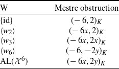
We now give a description of the Mestre obstruction in each case.
Proposition 5·1. For each subgroup W of the Atkin–Lehner group
 $\mathrm{AL}( {\mathcal X} ^6)$
, outside of finitely many j, the Mestre obstruction on
 $C^6_{W}$
can be described by the Hilbert symbol given in Table 1.
Mestre obstructions on
 $C_W^{6}$
, where x and y are as in Equation (5·2) and Equation (5·3) in each respective case

Table 1. Long description
A table titled ‘Mestre obstruction’ presents values for different subgroups of the Atkin-Lehner group. The table has two columns: the first column lists the subgroups, and the second column provides the corresponding Mestre obstruction values. The subgroups listed are id, w2, w3, w6, and AL(4^6). The Mestre obstruction values are (-6, 2)K for id, (-6x, 2)K for w2, (-6x, 2vx)K for w3, (-6, -2y)K for w6, and (-6x, 2y)K for AL(4^6).
Proof. By [
Reference Baba and Granath2
, proposition 3·12 and proposition 3·13], the Mestre obstruction to a curve C, corresponding to a point of
 $C^6$
, with rational Igusa invariants being defined over a number field K can be described by the Hilbert symbol
 \begin{equation}(\!-6j, -2(27j+16))_K\end{equation}
outside of the finitely many j such that the corresponding curve has extra automorphisms (specifically,
 $j = -16/27$
corresponding to the genus 2 curve
 $C_{(-24)}$
with
 $-24$
-CM and
 $j = 81/64$
corresponding to the genus 2 curve
 $C_{(-19)}$
with
 $-19$
-CM from [
Reference Baba and Granath2
, section 3·3]).
By our expression Equation (5·1) for the canonical ring
 $R^6_{\{\mathrm{id}\}}$
, we have
 $h_{12}^2+3h_6^4 + h_4^6=0$
. Also, we have by definition that
 $j=16h_6^4/9h_4^6$
. Therefore, we can rewrite the Mestre obstruction as follows:
 \begin{align*} \left(\!-6\frac{16h_6^4}{9h_4^6}, -2\left(27\frac{16h_6^4}{9h_4^6}+16\right)\right)_K &=(\!-6(16h_6^4), -2(27(16h_6^4)-16(9h_4^6))_K\\ &=(\!-6,-2(3h_6^4 + h_4^6))_K\\ &=(\!-6,2 h_{12}^2)_K\\ &=(\!-6,2)_K.\end{align*}
The other cases are similar, starting with Equation (5·5) and using the relations from the expressions Equation (5·2) and Equation (5·3) for the canonical rings.
Let
 $\pi\;:\;\mathcal{B}\to\mathbb{P}^1_j$
be the conic bundle corresponding to the Mestre obstruction on
 $C_{W}^6$
. We have the following commutative diagram:

Recall from the introduction that we define the function
 $\overline{\mathcal{N}}^6(W,K,B)$
to be that which counts, up to isomorphism over
 $\overline{K}$
, curves C in
 $C_{W}^6(K)$
which have a model over K and satisfy
 $\overline{\operatorname{Ht}}(C)\leq B$
.
Theorem 5·2. We have that
 \[\mathcal{\overline{N}}^6(W,K,B)\ll\begin{cases} B^2/\log(B) &\text{ if } W\in\{\mathrm{AL}( {\mathcal X} ^6),\langle w_3\rangle\}, \\ B^2/\log(B)^{1/2} &\text{ if } W\in\{\langle w_2\rangle, \langle w_6\rangle\},\\ B^2 &\text{ if } W=\{\mathrm{id}\} \text{ and } (\!-6,2)_K=1, \\ 0 &\text{ if } W=\{\mathrm{id}\} \text{ and } (\!-6,2)_K=-1.\end{cases}\]
These bounds are sharp when
 $K=\mathbb{Q}$
or
 $W=\{\mathrm{id}\}$
.
Proof. Note that
 $ {\mathscr J}$
extends to a morphism on all of
 $ {\mathbb P}^1$
. For
 $W\neq \{\mathrm{id}\}$
we apply Proposition 4·1 with
 $\varphi= {\mathscr J}$
. By the definition of
 $ {\mathscr J}$
we see that
 $\delta=1$
. Although the Mestre obstructions computed in Proposition 5·1 ignore finitely many points in
 $\mathbb{P}^1_j$
(i.e., finitely many curves in
 $C^{6}_{W}$
), this will not affect our asymptotic results. We now compute
 $\Delta(\pi)$
. Note that the smooth fibers of
 $\pi$
will only have a single irreducible component, and thus
 $\delta_x(\pi)=1$
in these cases. It remains to study the geometrically reducible fibers. From Proposition 5·1 we have that the conic bundle
 $\pi\;:\;\mathcal{B}\to \mathbb{P}^1_j$
has exactly two reducible fibers when
 $W=\mathrm{AL}( {\mathcal X} ^{6})$
and exactly one reducible fiber when
 $W\in\{\langle w_2\rangle, \langle w_6\rangle\}$
. In each of these cases the reducible fiber
 $\pi^{-1}(x)_{\overline{K}}$
has two irreducible components and
 $\operatorname{Gal}(\overline{K}/K)$
acts transitively on these components, so that
 $\delta_x(\pi)=1/2$
. In the case
 $W=\langle w_3\rangle$
we have a single reducible component of multiplicity 2. Therefore
 $\delta_x(\pi)=0$
. It follows that
 \[ \Delta(\pi)=\begin{cases} 1 \text{ if } W\in \{\mathrm{AL}( {\mathcal X} ^{6}),\langle w_3\rangle\},\\ 1/2 \text{ if } W\in\{\langle w_2\rangle, \langle w_6\rangle\}. \end{cases} \]
Applying Proposition 4·1 gives the desired result.
When
 $W=\{\mathrm{id}\}$
we either have
 $(\!-6,2)_K=1$
, in which case the Mestre obstruction vanishes and the desired result follows from Proposition 4·1, or we have
 $(\!-6,2)_K=-1$
, in which case
 $C^6_{\mathrm{AL}( {\mathcal X} ^6)}(K)=\emptyset$
.
We now bound the number of K-isomorphism classes.
Theorem 5·3. We have that
 \[\mathcal{N}^6(W,K,B)\ll\begin{cases} B^2/\log(B) &\text{ if } W\in\{\mathrm{AL}( {\mathcal X} ^6),\langle w_3\rangle\}, \\ B^2/\log(B)^{1/2} &\text{ if } W\in\{\langle w_2\rangle, \langle w_6\rangle\},\\ B^2 &\text{ if } W=\{\mathrm{id}\} \text{ and } (\!-6,2)_K=1, \\ 0 &\text{ if } W=\{\mathrm{id}\} \text{ and } (\!-6,2)_K=-1.\end{cases}\]
These bounds are sharp when
 $K= {\mathbb Q}$
or
 $W=\{\mathrm{id}\}$
.
Proof. From [
Reference Baba and Granath2
, proposition 3·12] there are finitely many curves corresponding to points of
 $C^6_W$
with geometric automorphism group
 $C_2\times C_2$
, and outside of these exceptions the geometric automorphism group is
 $C_2$
. From Proposition 3·2 the contribution to
 $ {\mathcal N} ^6(W,K,B)$
from curves with
 $\operatorname{Aut}_{\overline{K}}(C)\cong C_2\times C_2$
is O(B). From Proposition 3·2, Theorem 5·2, and Lemma 3·5, the contribution from curves with
 $\operatorname{Aut}_{\overline{K}}(C)\cong C_2$
gives the bounds in the statement of the theorem.
5·4. The discriminant 10 case
We first describe the stacky geometry of the Atkin–Lehner quotients
 $ {\mathcal X} ^{10}_{W}$
. For each W the stack
 $ {\mathcal X} ^{10}_{W}$
has a generic
 $\mu_2$
-gerbe. Rigidifying along this gerbe we get a stacky curve
 . Let
 $v_i$
denote the number of
 $\mu_i$
-stacky points of
 , and set
 $s_k\stackrel{\operatorname{def}}{=} \dim(H^0({\mathcal X} ^{10}_{W},\Omega^{\otimes k}))$
. In this case we will only have
 $\mu_2$
-stacky points and
 $\mu_3$
-stacky points. As we are in the genus 0 case, the dimension
 $s_k$
can be written in terms of
 $v_2$
and
 $v_3$
as follows for even weight
 $k \gt 2$
[
Reference Shimura31
, theorem 2·24]:
 \begin{equation}s_k=1-k + v_2 \left\lfloor \frac{k}{4} \right\rfloor + v_3 \left\lfloor \frac{k}{3} \right\rfloor + v_4 \left\lfloor \frac{3k}{8} \right\rfloor + v_6 \left\lfloor \frac{5k}{12} \right\rfloor,\end{equation}
while
 $s_2 = 0$
. The curve
 $ {\mathcal X} ^{10}$
has 4 points with CM by discriminant
 $-3$
and has no
 $-4$
-CM points, as
 $\mathbb{Q}(i)$
does not split the quaternion algebra over
 $\mathbb{Q}$
of discriminant
 $D=10$
. Each involution
 $w_m$
has 2 fixed points:
 $w_2$
has two fixed points which are the
 $-8$
-CM points on this curve,
 $w_5$
fixes the
 $-20$
-CM points, and
 $w_{10}$
fixes the
 $-40$
-CM points. We compute Table 2, analogous to that given in [
Reference Baba and Granath2
, section 3·1] in the
 $D=6$
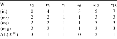
case.
Number
 $v_n$
of
 $\mu_n$
-stacky points and dimension
 $s_m$
of the space of weight m modular forms on
 $ {\mathcal X} ^{10}_W$

Table 2. Long description
A table with 5 rows and 7 columns. The columns are labeled as follows: id, v2, v3, s4, s6, s12, and s18. The rows are labeled as follows: id, {w2}, {w5}, {w10}, and AL(x^10). Row 1: id, 0; v2, 4; v3, 1; s4, 3; s6, 5; s12, 7. Row 2: id, 2; v2, 2; v3, 1; s4, 1; s6, 3; s12, 3. Row 3: id, 2; v2, 2; v3, 1; s4, 1; s6, 3; s12, 3. Row 4: id, 2; v2, 2; v3, 1; s4, 1; s6, 3; s12, 3. Row 5: id, 3; v2, 1; v3, 1; s4, 0; s6, 2; s12, 1.
From Table 2 we can fix a weight 4 modular form
 $g_4$
and weight 6 modular forms
 $g_6, h_6$
and
 $k_6$
such that the Atkin–Lehner involutions act as follows:
 \begin{align*} & g_4=w_2(g_4)=w_5(g_4)=w_{10}(g_4)\\[5pt] & g_6=w_2(g_6)=-w_5(g_6)=-w_{10}(g_6)\\[5pt] & h_6=-w_2(h_6)=w_5(h_6)=-w_{10}(h_6)\\[5pt] & k_6=-w_2(k_6)=-w_5(k_6)=w_{10}(k_6).\end{align*}
As noted in [ Reference Baba and Granath2 , section 4], we may normalise these forms so that
 \[g_6^2+2h_6^2+k_6^2=0 \qquad \text{and} \qquad 4g_4^3+27h_6^2+k_6^2=0.\]
These forms generate the ring of modular forms corresponding to
 $ {\mathcal X} ^{10}$
. With these relations, and the observation that in this case
 \[s_{k+12} = s_k+4,\]
we compute the canonical ring for each Atkin–Lehner quotient:
 \begin{align*} R_{\{\mathrm{id}\}}^{10}&\cong \mathbb{Q}[g_4,g_6,h_6,k_6]/\big(g_6^2+2h_6^2+k_6^2, 4g_4^3+27h_6^2+k_6^2\big)\\ R^{10}_{\langle w_2\rangle} &\cong \mathbb{Q}[g_4, g_6,h_6k_6]/\big(32g_4^6-116g_4^3g_6^2+27g_6^4+625(h_6k_6)^2\big)\\ &\cong \mathbb{Q}[x,y,z]/(32x^6-116x^3y^2+27y^4+625z^2) \\ R^{10}_{\langle w_5\rangle} &\cong \mathbb{Q}[g_4, h_6,g_6k_6]/\big(16g_4^6+208g_4^3h_6^2+675h_6^4+(g_6k_6)^2\big)\nonumber\\ &\cong \mathbb{Q}[x, y,z]/(16x^6+208x^3y^2+675y^4+z^2)\nonumber\\ R^{10}_{\langle w_{10}\rangle} &\cong \mathbb{Q}[g_4, k_6,g_6h_6]/\big(32g_4^6-92g_4^3k_6^2-25k_6^4+729(g_6h_6)^2\big)\nonumber\\ &\cong \mathbb{Q}[x, y,z]/(32x^6-92x^3y^2-25y^4+729z^2)\nonumber\\ R^{10}_{W}&\cong \mathbb{Q}[g_4, g_6^2,g_6h_6k_6]/\big(352g_4^6g_6^4-172g_4^3g_6^4+21g_6^6-(g_6h_6k_6)^2\big)\nonumber\\ &\cong \mathbb{Q}[x, y,z]/(32x^6y-116x^3y^2+27y^3+625z^2). \end{align*}
We give one example of the above computations, with the rest being similar.
Example 5·4. We indeed note that
 $R_{\langle w_2 \rangle}^{10}$
has minimal generating set
 $\{g_4, g_6, h_6k_6\}$
; each of these generators is fixed by the action of
 $w_2$
, no two are scalar-multiples of one-another, and our relations and dimension formula above show that any other form fixed by
 $w_2$
is in the ideal they generate. Using the relations among the generators of
 $R^{10}_{\mathrm{id}}$
, we can eliminate
 $k_6$
and
 $h_6$
, respectively, to get the relations
 \[ 25h_6^2 = g_6^2 - 4g_4^3 \qquad \text{ and } \qquad 25k_6^2 = 8g_4^3-27g_6^2. \]
Now using these relations, we compute
 \begin{align*} 625(h_6k_6)^2 &= (g_6^2-4g_4^3)\big(8g_4^3-27g_6^2\big) \\ &= -32g_4^6 + 116g_4^3g_6^2 - 27g_6^4. \end{align*}
This confirms the relation noted in
 $R^{10}_{\langle w_2 \rangle}$
in Equation (5·8). Furthermore, with our chosen generators the ideal of relations for this ring is generated by a single element, and it is clear from the relations on
 $R^{10}_{\text{id}}$
that there does not exist a relation between
 $g_4,g_6$
and
 $h_6k_6$
in lower degree.
Let j denote the weight zero modular form
 $g_4^3/g_6^2$
. From [
Reference Baba and Granath2
, proposition 4·2, proposition 4·6] j induces an isomorphism
 $j\;:\;C^{10}\to\mathbb{P}^1-\{0,\infty\}$
. Set
 \begin{align*} J_2&\stackrel{\operatorname{def}}{=} 12j^2-16j+12,\\ J_4&\stackrel{\operatorname{def}}{=} 6j^4-16j^3+6j^2-16j+6,\\ J_6 &\stackrel{\operatorname{def}}{=} 4j^6-16j^5+32j^3-8j^2-16j+4,\\ J_{10}&\stackrel{\operatorname{def}}{=} j^4.\end{align*}
This defines a morphism
 \begin{align*} {\mathscr J}\;:\; \mathbb{P}^1-\{0,\infty\} &\to {\mathcal P}(1,2,3,5)\\j &\mapsto [J_2 \;:\; J_4 \;:\; J_6 \;:\; J_{10}].\end{align*}
In the same way as Equation (5·4), we may write the morphism
 $ {\mathscr J}$
in terms of homogeneous polynomials by setting
 $j=u/v$
and homogenising with respect to the weights.
Using [
Reference Baba and Granath2
, proposition 4·4], we compute the Mestre obstruction on each
 $C^{10}_W$
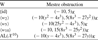
in the same way as in Proposition 5·1.
Proposition 5·5. For each subgroup W of the Atkin–Lehner group
 $\mathrm{AL}( {\mathcal X} ^{10})$
, outside of finitely many j, the Mestre obstruction on
 $C^{10}_{W}$
can be described by the Hilbert symbol given in Table 3.
Mestre obstructions on
 $C_W^{10}$
, where x and y are as in Equation (5·8) in each respective case

Table 3. Long description
A table showing Mestre obstructions for different subgroups of the Atkin-Lehner group. The table has 5 rows and 2 columns. The columns are labeled ‘W’ and ‘Mestre obstruction’. The rows are labeled with different subgroups of the Atkin-Lehner group. The values in the ‘Mestre obstruction’ column are given in terms of mathematical expressions involving x and y. Row 1: id, (-10, 5)K. Row 2: w2, (-10(ch^2 - 4ch^3), 5(ch^3 - 27y^2))K. Row 3: w5, (-10(25y^2 - 4ch^3), 5)K. Row 4: w10, (-10, 15(8ch^3 - 25y^2))K. Row 5: AL(4^10), (-10(y - 4ch^3), 5(ch^3 - 27y^2))K.
Letting
 $\pi\;:\;\mathcal{B}\to\mathbb{P}^1$
denote the conic bundle corresponding to the Mestre obstruction on
 $C^{10}_{W}$
, we obtain a commutative diagram analogous to Equation (5·6).
Theorem 5·6. We have that
 \[\overline{\mathcal{N}}^{10}(W,K,B)\ll\begin{cases} B/\log(B) &\text{ if } W\in\{\mathrm{AL}( {\mathcal X} ^{10}),\langle w_2\rangle\}, \\[5pt] B/\log(B)^{1/2} &\text{ if } W\in\{\langle w_5\rangle, \langle w_{10}\rangle\},\\[5pt] B &\text{ if } W=\{\mathrm{id}\} \text{ and } (\!-10,5)_K=1, \\[5pt] 0 &\text{ if } W=\{\mathrm{id}\} \text{ and } (\!-10,5)_K=-1.\end{cases}\]
These bounds are sharp when
 $K=\mathbb{Q}$
or
 $W=\{\mathrm{id}\}$
.
Proof. Note that
 $ {\mathscr J}$
extends to a morphism on all of
 $ {\mathbb P}^1$
. For
 $W\neq \{\mathrm{id}\}$
we apply Proposition 4·1 with
 $\varphi= {\mathscr J}$
. By the definition of
 $ {\mathscr J}$
we see that
 $\delta=2$
. We now compute
 $\Delta(\pi)$
. Note that the smooth fibers of
 $\pi$
will only have a single irreducible component, and thus
 $\delta_x(\pi)=1$
for these fibers. It remains to study the geometrically reducible fibers. From Proposition 5·5, we have that the conic bundle
 $\pi\;:\;\mathcal{B}\to \mathbb{P}^1_j$
has exactly two reducible fibers when
 $W\in\{\mathrm{AL}( {\mathcal X} ^{10}),\langle w_2\rangle\}$
and exactly one reducible fiber when
 $W\in\{\langle w_5\rangle, \langle w_{10}\rangle\}$
. In each of these cases the reducible fiber
 $\pi^{-1}(x)_{\overline{K}}$
has two irreducible components and
 $\operatorname{Gal}(\overline{K}/K)$
acts transitively on these components, so that
 $\delta_x(\pi)=1/2$
. It follows that
 \[ \Delta(\pi)=\begin{cases} 1 \text{ if } W\in \{\mathrm{AL}( {\mathcal X} ^{10}),\langle w_2\rangle\},\\[5pt] 1/2 \text{ if } W\in\{\langle w_5\rangle, \langle w_{10}\rangle\}. \end{cases} \]
Applying Proposition 4·1 gives the desired result.
When
 $W=\{\mathrm{id}\}$
we either have
 $(\!-10,5)_K=1$
, in which case the Mestre obstruction vanishes and the desired result follows from Proposition 4·1, or we have
 $(\!-10,5)_K=-1$
, in which case
 $C^{10}_{\{\mathrm{id}\}}(K)=\emptyset$
.
We now count K-isomorphism classes.
Theorem 5·7. We have that
 \[\mathcal{N}^{10}(W,K,B)\ll\begin{cases} B &\text{ if } W\in\{\mathrm{AL}( {\mathcal X} ^{10}),\langle w_2\rangle\}, \\ B\log(B)^{1/2} &\text{ if } W\in\{\langle w_5\rangle, \langle w_{10}\rangle\},\\ B\log(B) &\text{ if } W=\{\mathrm{id}\} \text{ and } (\!-10,5)_K=1, \\ 0 &\text{ if } W=\{\mathrm{id}\} \text{ and } (\!-10,5)_K=-1.\end{cases}\]
Proof. From [
Reference Baba and Granath2
, proposition 4·11] there are finitely many curves corresponding to points of
 $C^{10}_W$
with geometric automorphism group
 $C_2\times C_2$
or
 $D_4$
, and outside of these exceptions the automorphism group is
 $C_2$
. From Proposition 3·2 the contribution to
 $ {\mathcal N} ^{10}(W,K,B)$
from curves with
 $\operatorname{Aut}_{\overline{K}}(C)\cong C_2\times C_2$
is o(B). From Proposition 3·4 the contribution from curves with
 $\operatorname{Aut}_{\overline{K}}(C)\cong D_4$
is also o(B). From Proposition 3·2, Theorem 5·2 and Lemma 3·5, the contribution from curves with
 $\operatorname{Aut}_{\overline{K}}(C)\cong C_2$
gives the bounds in the statement of the theorem.
5·5. The discriminant 22 case
Assume the same setup and notation as in the
 $D=10$
case. The curve
 $ {\mathcal X} ^{22}$
has 2 geometric points with CM by discriminant
 $-4$
and 4 geometric points with CM by discriminant
 $-3$
. As
 $2 \mid 22$
, we will encounter
 $\mu_4$
-stacky points on the quotient by
 $\langle w_2 \rangle$
and on the full quotient. Each involution
 $w_m$
has 2 fixed points:
 $w_2$
fixes the two
 $-4$
-CM points, and
 $w_{11}$
and
 $w_{22}$
fix the
 $-11$
-CM and
 $-88$
-CM points, respectively, on
 $ {\mathcal X} ^{22}$
.
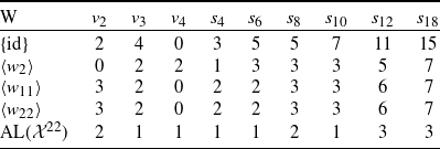
Table 4 displays counts of stacky points and dimensions of spaces of modular forms on each quotient in even weights up to 18.
Number
 $v_n$
of
 $\mu_n$
-stacky points and dimension
 $s_m$
of weight m modular forms on
 $ {\mathcal X} ^{22}_W$

Table 4. Long description
A table with 6 rows and 10 columns. The columns are labeled as v2, v3, v4, s4, s6, s8, s10, s12, and s18. The rows are labeled as id, {w2}, {w11}, {w22}, and AL(χ22). Row 1: id, 2, 4, 0, 3, 5, 5, 7, 11, 15. Row 2: {w2}, 0, 2, 2, 1, 3, 3, 3, 5, 7. Row 3: {w11}, 3, 2, 0, 2, 2, 3, 3, 6, 7. Row 4: {w22}, 3, 2, 0, 2, 2, 3, 3, 6, 7. Row 5: AL(χ22), 2, 1, 1, 1, 1, 2, 1, 3, 3.
From this information, we fix weight 4 forms
 $f_{4,i}$
for
 $i \in \{1,2,4\}$
generating the space of weight 4 forms on
 $ {\mathcal X} ^{22}$
and weight 6 forms
 $f_{6,j}$
for
 $j \in \{1,2,3,4,5\}$
generating the space of weight 6 forms on
 $ {\mathcal X} ^{22}$
such that
 \begin{align*} f_{4,1} &= w_2(\,f_{4,1}) = w_{11}(\,f_{4,1}) = w_{22}(\,f_{4,1}), \\ f_{4,2} &= -w_2(\,f_{4,2}) = w_{11}(\,f_{4,2}) = -w_{22}(\,f_{4,2}), \\ f_{4,3} &= -w_2(\,f_{4,3}) = -w_{11}(\,f_{4,3}) = w_{22}(\,f_{4,3}), \\ f_{6,1} &= w_2(\,f_{6,1}) = -w_{11}(\,f_{6,1}) = -w_{22}(\,f_{6,1}), \\ f_{6,2} &= w_2(\,f_{6,2}) = -w_{11}(\,f_{6,2}) = -w_{22}(\,f_{6,2}), \\ f_{6,3} &= -w_2(\,f_{6,3}) = w_{11}(\,f_{6,3}) = -w_{22}(\,f_{6,3}) ,\\ f_{6,4} &= w_2(\,f_{6,4}) = w_{11}(\,f_{6,4}) = w_{22}(\,f_{6,4}) \text{ and }\\ f_{6,5} &= -w_2(\,f_{6,5}) = -w_{11}(\,f_{6,5}) = w_{22}(\,f_{6,5}).\end{align*}
As in the
 $D=10$
case, it follows from the dimension formula Equation (5·7) that the full ring of modular forms corresponding to
 $ {\mathcal X} ^{22}$
is generated by the weight 4 and weight 6 forms
 $g_4,h_4,k_4,g_6,h_6,j_6,k_6,$
and
 $\ell_6$
. Moreover, in this case we have
 \[s_{k+12} = s_{k} + 10.\]
The dimensions of these spaces of forms make it difficult to determine all of the relations without further information, compared to the
 $D=6,10$
cases. Fortunately, these are worked out in thesis work of Joan Nualart Riera [
Reference Nualart Riera22
] using explicit computations of expansions of automorphic forms around CM points. Our notation for the generators has been chosen to match that in [
Reference Nualart Riera22
], and the relations are determined in [
Reference Nualart Riera22
, proposition 6·17] to be as follows:
 \begin{alignat*}{3} 0 &= r_1 \stackrel{\operatorname{def}}{=} 11 f_{4,3}^2+f_{4,1}^2+11f_{4,2}^2 , \quad &&0 = r_{13} \stackrel{\operatorname{def}}{=} 176f_{4,1}^2f_{4,2} - 121f_{6,3}f_{6,4} - 27f_{6,2}f_{6,5} , \\ 0 &= r_2 \stackrel{\operatorname{def}}{=} -f_{4,2}f_{6,2} + f_{4,1}f_{6,5} , \qquad &&0 = r_{14} \stackrel{\operatorname{def}}{=} -f_{6,5}^2+f_{6,1}f_{6,2} , \\ 0 &= r_3 \stackrel{\operatorname{def}}{=} -f_{4,2}f_{6,5} + f_{4,1}f_{6,1} , \qquad &&0 = r_{15} \stackrel{\operatorname{def}}{=} -f_{6,4}f_{6,5} + f_{6,1}f_{6,3} , \\ 0 &= r_4 \stackrel{\operatorname{def}}{=} f_{4,2}f_{6,4} - f_{4,3}f_{6,1} , \qquad &&0 = r_{16} \stackrel{\operatorname{def}}{=} f_{6,2}f_{6,4} - f_{6,3}f_{6,5} , \\ 0 &= r_5 \stackrel{\operatorname{def}}{=} f_{4,1}f_{6,4} - f_{4,3}f_{6,5} , \qquad &&0 = r_{17} \stackrel{\operatorname{def}}{=} -11f_{6,3}^2 + 121f_{6,4}^2 - f_{6,2}^2 + 121f_{6,1}^2 , \\ 0 &= r_6 \stackrel{\operatorname{def}}{=} -f_{4,2}f_{6,3} + f_{4,1}f_{6,4} , \qquad &&0 = r_{18} \stackrel{\operatorname{def}}{=} 11f_{6,3}f_{6,4} + f_{6,2}f_{6,5} + 11f_{6,1}f_{6,5} , \\ 0 &= r_7 \stackrel{\operatorname{def}}{=} f_{4,1}f_{6,3} - f_{4,3}f_{6,2} , \qquad &&0 = r_{19} \stackrel{\operatorname{def}}{=} 11f_{6,3}^2+f_{6,2}^2+11f_{6,5}^2 , \\ 0 &= r_8 \stackrel{\operatorname{def}}{=} 11f_{4,3}f_{6,4} + f_{4,1}f_{6,5} + 11f_{4,2}f_{6,1} , \qquad &&0 = r_{20} \stackrel{\operatorname{def}}{=} 176f_{4,1}^3 - 121f_{6,3}^2 - 27f_{6,2}^2 , \\ 0 &= r_9 \stackrel{\operatorname{def}}{=} 11f_{4,3}f_{6,3}+f_{4,1}f_{6,2}+11f_{4,2}f_{6,5} , \\ 0 &= r_{10} \stackrel{\operatorname{def}}{=} 1936f_{4,1}f_{4,2}^2 + 297f_{6,3}^2 - 1331f_{6,4}^2+27f_{6,2}^2 , \\ 0 &= r_{11} \stackrel{\operatorname{def}}{=} 176f_{4,1}f_{4,2}f_{4,3} - 16f_{6,2}f_{6,4}+121f_{6,1}f_{6,4} , \\ 0 &= r_{12} \stackrel{\operatorname{def}}{=} 176f_{4,1}^2f_{4,3}-16f_{6,2}f_{6,3}+121f_{6,1}f_{6,3} .\end{alignat*}
Let
 $\mathcal{R} = \{r_i \mid 1 \leq i \leq 20\}$
denote the complete set of 20 relations among the generators. The canonical rings for each quotient are then:
 \begin{align*}R_{\{\mathrm{id}\}}^{22} &\cong \mathbb{Q}[\,f_{4,1},f_{4,2},f_{4,3},f_{6,1},f_{6,2},f_{6,3},f_{6,4},f_{6,5}]/\mathcal{R} \\R_{\langle w_2 \rangle}^{22} &\cong \mathbb{Q}[\,f_{4,1},f_{4,2}^2,f_{4,2}f_{4,3},f_{6,1},f_{6,2},f_{6,4}]/\mathcal{R}_{\langle w_2 \rangle} \\R_{\langle w_{11} \rangle}^{22} &\cong \mathbb{Q}[\,f_{4,1},f_{4,2},f_{6,3},f_{6,4},f_{6,1}^2]/\mathcal{R}_{\langle w_{11} \rangle}\\R_{\langle w_{22} \rangle}^{22} &\cong \mathbb{Q}[\,f_{4,1},f_{4,3},f_{6,4},f_{6,5}]/\mathcal{R}_{\langle w_{22} \rangle} \\R_{W}^{22} &\cong \mathbb{Q}[\,f_1^2,f_2^2,f_{6,4},f_{4,2}f_{4,3}f_{6,1},f_{4,2}f_{4,3}f_{6,2},f_{4,2}f_{6,1}f_{6,5},f_{4,2}f_{6,2}f_{6,5},f_{4,3}f_{6,1}f_{6,3}, \\& \qquad \qquad f_{4,3}f_{6,2}f_{6,3},f_{6,1}f_{6,3}f_{6,5},f_{6,2}f_{6,3}f_{6,5}]/\mathcal{R}_{\mathrm{AL}( {\mathcal X} ^{22})},\end{align*}
where, for each non-trivial subgroup
 $W \leq \mathrm{AL}( {\mathcal X} ^{22})$
, we write
 $\mathcal{R}_W$
for the ideal of relations in R fixed by W. (While identifying explicit generators for the canonical ring of each quotient will be useful in what follows, writing down a full set of generators for each
 $\mathcal{R}_W$
appears to be computationally difficult and will not be necessary.)
For a wide range of indefinite quaternion discriminants D, Igusa invariants and the Mestre obstruction on
 $ {\mathcal X} ^{D}$
are worked out explicitly in [
Reference Lin and Yang16
] in terms of a specified Hauptmodul on the full quotient. In terms of a specific hauptmodul j on
 $ {\mathcal X} ^{22}/\mathrm{AL}( {\mathcal X} ^{22})$
, Igusa invariants for
 $C^{22}$
can be derived from [
Reference Lin and Yang16
]; they are
 \begin{align*} J_2 &\stackrel{\operatorname{def}}{=} 2^2 (3 j^{5} + 5 j^{4} + 23 j^{3} + 10 j^{2} + 4 j + 3), \\ J_4 &\stackrel{\operatorname{def}}{=} 2 (3j^{10} + 7j^{9} + 27j^{8} + 57j^{7} + 251j^{6} + 261j^{5} + 120j^{4} + 27j^{3} + 4j^{2} + 8j + 3), \\ J_6 &\stackrel{\operatorname{def}}{=} -2^{2} \cdot (j^{5} - 3j^{4} - 3j^{3} - 6j^{2} - 4j - 1)\\ &\qquad \cdot (j^{10} + 5j^{9} - 9j^{8} - 69j^{7} - 87j^{6} - 89j^{5} - 36j^{4} + 17j^{3} + 12j^{2} - 1), \\ J_{10} &\stackrel{\operatorname{def}}{=} -(j - 1)^{4} \cdot j^{6} \cdot (j + 1)^{12}.\end{align*}
The Igusa invariants induce a morphism
 \begin{align*} {\mathscr J}\;:\; \mathbb{P}^1-\{0,\infty\} &\to {\mathcal P}(1,2,3,5)\\j &\mapsto [J_2 \;:\; J_4 \;:\; J_6 \;:\; J_{10}].\end{align*}
In the same way as Equation (5·4), we may write the morphism
 $ {\mathscr J}$
in terms of homogeneous polynomials by setting
 $j=u/v$
and homogenising with respect to the weights.
The Mestre obstruction on
 $ {\mathcal X} ^{22}$
is given (in [
Reference Lin and Yang16
, table 4]) by the symbol
 \[\left( -22j, -11(16j + 11) \right).\]
To make use of the explicit computation of the Mestre obstruction, as well as the above explicit computation of canonical rings on each quotient, we will relate this j from [
Reference Lin and Yang16
] to the Hauptmodul
 $t_{22}^+$
on the full quotient defined in [
Reference Nualart Riera22
, theorem 2·4].
Lemma 5·8. The Hauptmoduln j and
 $t_{22}^+$
satisfy the relation
 \[ j = \dfrac{11}{16(t_{22}^+-1)} . \]
Proof. Each of j and
 $t_{22}^+$
is a Hauptmodul on
 $ {\mathcal X} ^{22}/\mathrm{AL}( {\mathcal X} ^{22})$
, so there are a, b, c, d with
 \[ t_{22}^+ = \dfrac{aj + b}{cj + d}. \]
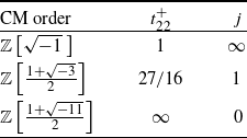
Knowing the values of t and j at three distinct points will then determine the relationship. Specifically, we use values at the three CM points that specify j in [
Reference Lin and Yang16
, table 2]. The values of
 $t_{22}^+$
at these same CM points are given in [
Reference Nualart Riera22
, theorem 3·1], and we copy the values of each in Table 5.
Values of Hauptmoduln at some CM points of
 $ {\mathcal X} ^{22}$

Table 5. Long description
A table with three rows and three columns. The columns are labeled CM order, t22, and j. The rows are as follows: Row 1: CM order, Z; t22, 1; j, infinity. Row 2: CM order, Z; t22, 27/16; j, 1. Row 3: CM order, Z; t22, infinity; j, 0.
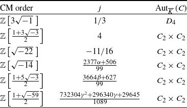
Proposition 5·9. Let
 $\alpha$
be such that
 \begin{equation*} 121+1210\alpha+2377\alpha^2=0, \end{equation*}
let
 $\beta$
be such that
 \begin{equation*} 121+1331\beta+3664\beta^2 \end{equation*}
and let
 $\gamma$
be such that
 \begin{equation*} 1331+37389\gamma+296340\gamma^2 + 732304\gamma^3. \end{equation*}
Then Table 6 lists all points of
 $C_W^{22}$
corresponding to genus two curves whose geometric automorphism group
 $\operatorname{Aut}_{\overline{K}}(C)$
is not isomorphic to the cyclic group of order two
 $C_2$
.
Proof. The curves with extra automorphism are given in [ Reference Nualart Riera22 , proposition 3·16]. The corresponding values of j can be determined from [ Reference Nualart Riera22 , proposition 3·16], [ Reference Nualart Riera22 , theorem 3·10], and Lemma 5·8. The geometric automorphism groups are then found by computing the corresponding Igusa invariants.
Using the definitions given in [
Reference Nualart Riera22
, proposition 6·17] for the generators of the rings of modular forms in terms of
 $t_{22}^+$
, we find that
 \[ t_{22}^+ = -\dfrac{f_{6,4}^2}{f_{6,1}^2}.\]
Therefore, from Lemma 5·8, we have
 \begin{equation}j = -\dfrac{11f_{6,1}^2}{16(\,f_{6,1}^2+f_{6,4}^2)}.\end{equation}
We next compute the Mestre obstructions on each quotient.
Points of
 $ {\mathcal C} ^{22}$
with extra automorphisms

Table 6. Long description
A table listing points of with extra automorphisms for genus two curves. The table has 6 rows and 3 columns. The columns are labeled CM order, j, and Aut K (C). Row 1: CM order Z, 3 root -1, j 1/3, Aut K (C) D 4. Row 2: CM order Z, 1+3 root -3 over 2, j 4, Aut K (C) C 2 x C 2. Row 3: CM order Z, root -22, j -11/16, Aut K (C) C 2 x C 2. Row 4: CM order Z, root -14, j 2377 root 4+506 over 99, Aut K (C) C 2 x C 2. Row 5: CM order Z, 1+5 root -3 over 2, j 3664 root 4+627 over 99, Aut K (C) C 2 x C 2. Row 6: CM order Z, 1+ root -59, j 732304 root 4+296340 root 3+29645 over 1089, Aut K (C) C 2 x C 2.
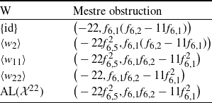
Proposition 5·10. For each subgroup W of the Atkin–Lehner group
 $\mathrm{AL}( {\mathcal X} ^{22})$
, outside of finitely many j, the Mestre obstruction on
 $C^{22}_{W}$
can be described by the Hilbert symbol given in Table 7.
Proof. On the top curve, we compute
 \begin{align*} &(\!-22j, -11(16j+11)) = \big( 2\big(\,f_{6,1}^2+f_{6,4}^2\big) , \big(\,f_{6,1}^2+f_{6,4}^2\big)\big(2f_{6,1}^2+f_{6,4}^2\big)\big) \\ &\qquad = \bigg( 2\big(11f_{6,3}^2+f_{6,2}^2\big), \big(11f_{6,3}^2+f_{6,2}^2\big)\bigg(\,f_{6,1}^2 + \frac{1}{121}(11f_{6,3}^2+f_{6,2}^2)\bigg)\bigg) \\ &\qquad = \big(\!-22, f_{6,5}^2-11f_{6,1}^2\big) \\ &\qquad = (\!-22 , f_{6,1}(\,f_{6,2} - 11 f_{6,1})). \end{align*}
The relations
 $r_{17}, r_{19}$
and
 $r_{14}$
used above are all fixed by the full Atkin–Lehner group. The only algebraic steps in our simplification that is not necessarily valid on each quotient is the identification of
 $f_{6,5}^2$
as a square in the canonical ring and factoring
 $f_{6,1}f_{6,2} - 11f_{6,1}^2$
. Note that
 $f_{6,5}^2$
is a square only for
 $W \in \{\{\mathrm{id}\}, \langle w_{22} \rangle \}$
. These observations give us the claimed symbols on each quotient in Table 7.
Mestre obstructions on
 $C_W^{22}$

Table 7. Long description
A table comparing Mestre obstructions for different subgroups of the Atkin-Lehner group. The table has 5 rows and 2 columns. The columns are labeled ‘W’ and ‘Mestre obstruction’. The rows are labeled with different subgroups: id, w2, w11, w22, and AL(22). The values in the ‘Mestre obstruction’ column are mathematical expressions involving f6,1, f6,2, and f1f6,1. Each row provides a specific expression for the corresponding subgroup.
In this case, we see that the Mestre obstruction on the top curve
 $ {\mathcal X} ^{22}$
over a fixed number field K is not constant, as it was for
 $D\in\{6,10\}$
. The non-split fibers in this case do not all correspond to rational points on the coarse space
 $X^{22}$
, as the curve has no
 $\mathbb{Q}$
-rational points. For this reason our counting result Proposition 4·1 does not give the correct count over all number fields. The non-split fibers occurring when
 $D\in\{6,10\}$
correspond to rational points with CM by certain imaginary quadratic orders of class number one on quotients
 $X^D/W$
by non-trivial subgroups
 $W \leq \mathrm{AL}( {\mathcal X} ^D)$
.
The residue field of the single quadratic point on
 $ {\mathcal X} ^{22}$
with CM by the order
 $\mathbb{Z}[({1+\sqrt{-11}})/{2}]$
is
 $\mathbb{Q}(\sqrt{-11})$
(which is its own Hilbert class field, as this is a class number 1 order).
Theorem 5·11. We have that
 \[\overline{\mathcal{N}}^{22}(W,K,B)\ll\begin{cases} B^{2/5}/\log(B)^{3/2} &\text{ if } W\in\{\langle w_2\rangle, \mathrm{AL}( {\mathcal X} ^{22})\} \\ &\text{ or if } W=\langle w_{11}\rangle \text{ and } \mathbb{Q}(\sqrt{-11}) \subseteq K,\\ B^{2/5}/\log(B) &\text{ if } W = \langle w_{22}\rangle \\ &\text{ or if } W=\{\mathrm{id}\} \text{ and } \mathbb{Q}(\sqrt{-11}) \subseteq K.\\ \end{cases}\]
Proof. Following the arguments of Theorem 5·2 and Theorem 5·6, we apply Proposition 4·1 with
 $\varphi= {\mathscr J}$
. From the definition of
 $ {\mathscr J}$
we see that
 $\delta=5$
. From Proposition 5·10, we see that the Mestre conic bundle
 $\pi\;:\;\mathcal{B}\to \mathbb{P}^1_j$
has exactly two reducible fibers for all W. These two fibers correspond to
 $f_{6,2}=11f_{6,1}$
and
 $f_{6,1}=0$
. Using the relations of the modular forms
 ${\mathcal R}$
, if
 $f_{6,2}=11f_{6,1}$
then
 $j=11/16$
. Using the relations also shows that if
 $f_{6,1}=0$
then
 $f_{6,4}=0$
. In order to find the corresponding value of j when
 $f_{6,1}=0$
we compute q-expansions of the modular forms
 $f_{6,1}$
and
 $f_{6,2}$
at the point with CM by
 $\mathbb{Z}\left[\frac{1+\sqrt{-11}}{2}\right]$
, which can be done using results in Nualart Riera’s thesis [
Reference Nualart Riera22
, proposition 6·17 and table 6·15]. Carrying out this computation shows that if
 $f_{6,1}=0$
then
 $j=0$
.
An assumption in Proposition 4·1 is that all the non-split fibers lie above rational points. Although
 $j=0$
is a rational point on
 $ {\mathbb P}^1_j$
, we ultimately care about counting the corresponding abelian surfaces. The point
 $j=0$
corresponds to the single quadratic point
 $z_{11}$
with CM by
 $\mathbb{Z}\left[\frac{1+\sqrt{-11}}{2}\right]$
on
 $ {\mathcal X} ^{22}$
. This CM point has residue field
 $\mathbb{Q}(\sqrt{-11})$
(moreover K is a field of definition for a QM abelian surface inducing
 $z_{11}$
if and only if
 $\mathbb{Q}(\sqrt{-11})\subseteq K$
by Jordan’s result [
Reference Jordan14
, theorem 2·1·3]). Each nontrivial Atkin–Lehner involution aside from
 $w_{11}$
acts on
 $z_{11}$
as complex conjugation, while
 $w_{11}$
fixes
 $z_{11}$
. We then have a single rational
 $-11$
-CM point on the quotient by W for
 $W \in \{\langle w_2 \rangle, \langle w_{22} \rangle, \mathrm{AL}( {\mathcal X} ^{22})\}$
which is elliptic of order 2 in the case of the full quotient, and a single quadratic
 $-11$
-CM point which is elliptic of order 2 on the quotient by
 $\langle w_{11} \rangle$
.
We now compute
 $\Delta(\pi)$
. If
 $W=\{\mathrm{id}\}$
and
 $\mathbb{Q}(\sqrt{-11}) \subseteq K$
, or if
 $W=\langle w_{22}\rangle$
, then the two reducible fibers each have two reducible components on which
 $\operatorname{Gal}(\overline{K}/K)$
acts transitively. Therefore
 $\Delta(\pi)=1/2+1/2=1$
.
If
 $W\in\{\langle w_2\rangle, \langle w_{11}\rangle, \mathrm{AL}( {\mathcal X} ^{22})\}$
then one of the reducible fibers has a single component of multiplicity 2, and the other reducible fiber has two components on which
 $\operatorname{Gal}(\overline{K}/K)$
acts transitively. Therefore
 $\Delta(\pi)=1+1/2=3/2$
.
We now count K-isomorphism classes.
Theorem 5·12. Assume that:
-
(i)
$W\in \{\langle w_2\rangle, \langle w_{22}\rangle, \mathrm{AL}( {\mathcal X} ^{22})\}$
or -
(ii)
$W\in \left\{ \{\mathrm{id}\}, \langle w_{11}\rangle\right\}$
and
$\mathbb{Q}(\sqrt{-11})\subseteq K$
.


Then
 \[\mathcal{N}^{22}(W,K,B)\asymp B.\]
Proof. From Proposition 5·9 there are finitely many curves corresponding to points of
 $C^{22}_W$
with geometric automorphism group
 $C_2\times C_2$
or
 $D_4$
, and outside of these exceptions the automorphism group is
 $C_2$
. From Proposition 3·2 the contribution to
 $ {\mathcal N} ^{22}(W,K,B)$
from curves with
 $\operatorname{Aut}_{\overline{K}}(C)\cong C_2\times C_2$
is o(B). From Proposition 3·4 the contribution from curves with
 $\operatorname{Aut}_{\overline{K}}(C)\cong D_4$
is also o(B). From Proposition 3·2, Theorem 5·11, and Lemma 3·5, the contribution from curves with
 $\operatorname{Aut}_{\overline{K}}(C)\cong C_2$
gives the estimate in the statement of the theorem.
Acknowledgements
This project came out of the 2023 American Mathematical Society Mathematics Research Community (MRC) on Explicit Computations with Stacks. The authors are extremely grateful for having the opportunity to be a part of this community. Many thanks to all the helpers and organisers of the MRC for putting on a wonderful workshop. Special thanks go to John Voight for his guidance and encouragement on this problem, as well as providing thoughtful feedback on an earlier draft of this paper. Thanks also to Arul Shankar for a helpful conversation about counting
 $D_4$
-octic extensions of number fields. Finally, we would like to thank the referees for their thoughtful comments and corrections.
Support for this project was provided by the National Science Foundation under Grant Number 1916439 for the 2023 summer AMS MRC. During this project T.P. was supported by National Science Foundation grant DMS-2303011. T.S. was supported during the project by FWO Vlaanderen and the Herschel Smith Fund. J.Y. was supported by National Science Foundation RTG grant DMS-2231565.


 CW6
 vn
 μn
 sm
 XW10
 CW10
 vn
 μn
 sm
 XW22
 X22
 C22
 CW22

 Open access

