I. INTRODUCTION
Two-port network stability has been discussed in a great deal of literature [Reference Woods1–Reference Edwards and Sinsky5]. Conventional stability parameters such as Rollet K and B parameters were used to discuss the unconditionally stable cases [Reference Rollett4]. The K and B parameters are algebraic combinations of S parameters and can be expressed as follows:
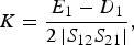

where D 1 and E 1 are defined as



K > 1 and the auxiliary condition B1 > 0 were used to identify unconditional stability in the ΓS plane. It can be shown that K > 1, B1 > 0 is equivalent to K > 1, B2 > 0 [Reference Edwards and Sinsky5, Reference Gonzalez6]; thus unconditional stability occurs in both the ΓS plane and the ΓL plane. The B 2, D 2, and E 2 parameters used in the ΓL plane can be formed by interchanging the subscripts (1 → 2 and 2 → 1). Edwards and Sinsky [Reference Edwards and Sinsky5] used a single geometrically derived parameter μ′ (or μ) to assess unconditional stability instead of the conventional K and B factors. They showed that μ′ > 1 (or μ > 1) is necessary and sufficient for a two-port network to be unconditionally stable, where


and where C 1 and C 2 are defined as


The formulae [Reference Gonzalez6] below are used to obtain the expressions in equaions (6)–(7):


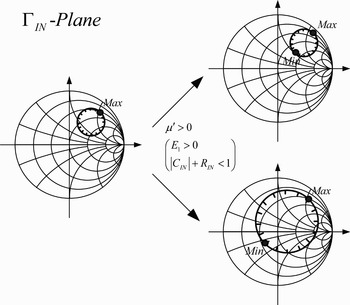
Unconditionally stable μ′ > 1 (or μ > 1) indicates that the stability circle (SC) is outside the unit smith chart (USC) in the ΓS (or ΓL) plane. Although μ′ > 1 (or μ > 1) provides a useful single stability parameter to replace the dual Rollet (K > 1) plus auxiliary condition (B 1 > 0), there exist other situations between SC and USC. As shown in Fig. 1, the condition of μ′ > 1 only determines that the maximum distance of SC is inside USC (|C IN| + R IN < 1), but the minimum distance is still unknown (in the ΓIN plane). One is unable to determine whether the origin of USC is inside SC or not. Therefore, another geometrically derived parameter ν′ (or ν) is presented in this paper to include all possible situations between SC and USC in the ΓS (or ΓIN) plane.
Two different stability conditions with only the discriminative parameter of μ′.

ν′ (or ν) is defined as


R S and C S can be expressed in terms of S parameters as explained in the Appendix. On substituting Equation (41) into Equation (6), the expression of μ′ becomes


We can also substitute Equation (A.13) into Equation (12). Thus, the expression for ν′ becomes


It is straightforward that |μ′| and |ν′| have geometrical meanings in the ΓS plane, and |ν′| is obviously larger than |μ′| · |ν′| is the maximum distance from SC to the origin of USC and |μ′| is the minimum distance from SC to the origin of USC in the ΓS plane, respectively. Moreover, the sign of μ′ determines whether the origin of USC is in the stable region or not. From Equation (12), ν′ is the opposite sign of D 1. It implies that the sign of ν′ can also determine whether the internal region of the SC (disk) is stable or the external region of the SC (disk complement) is stable. Therefore, two geometrically derived parameters, μ′ and ν′, have the concepts of position and stable region.
II. USING TWO GEOMETRICALLY DERIVED PARAMETERS TO CLASSIFY 12 SITUATIONS IN THE ΓS AND ΓIN PLANES
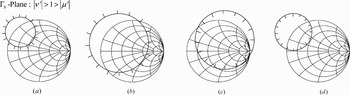
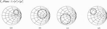
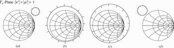
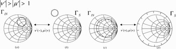
According to the μ′ and ν′ geometrical meanings, the geometrical relationship between SC and USC in the ΓS plane can be classified into 12 situations as illustrated in Figs 2–4. The region inside SC is stable if the tick goes inwards and the region outside SC is stable if the tick goes outwards for all the figures in this paper.
SC and USC in the ΓS plane when |ν′| > 1 > |μ′|. (a) ν′ < 0, μ′ >0. (b) ν′ < 0, μ′ < 0. (c) ν′ > 0, μ′ > 0. (d) ν′ > 0, μ′ < 0 (tick marks indicate the stable region).

SC and USC in the ΓS plane when 1 > |ν′| > |μ′|. (a) ν′ < 0, μ′ > 0. (b) ν′ < 0, μ′ < 0. (c) ν′ > 0, μ′ > 0. (d) ν′ > 0, μ′ < 0 (tick marks indicate the stable region).

SC and USC in the ΓS plane when |ν′| > |μ′| > 1. (a) ν′ < 0, μ′ > 0. (b) ν′ < 0, μ′ < 0. (c) ν′ > 0, μ′ > 0. (d) ν′ > 0, μ′ < 0 (tick marks indicate the stable region).

In the Appendix, the stable region (|ΓOUT| < 1) maps into a disk in the ΓS plane if D 1 < 0 and into a disk complement in the ΓS plane if D 1 > 0. From Equation (12), ν′ is positive if D1 < 0 and negative if D 1 > 0. It is easy to see from Equations (14) and (15) that in the case of ν′ > 0 (or ν′ < 0), the distance from the origin of USC to the center of SC is larger than the radius of SC in the ΓS plane when μ′ > 0 (or μ′ < 0) and the distance from the origin of USC to the center of SC is smaller than the radius of SC in the ΓS plane when μ′ < 0 (or μ′ > 0). The 12 situations can be grouped into three groups as follows:
1) If |ν′| > 1 > |μ′|, SC intersects USC in two points in the ΓS plane. As illustrated in Fig. 2, the four situations according to the signs of μ′ and ν′ correspond to |K| < 1 [Reference Edwards, Cheng and Sinsky7]. The geometrical relation between SC and USC provides useful insights and information for the conditionally stable design [Reference Edwards, Cheng and Sinsky7–Reference Edwards, Roddewig and Cheng9].
2) If 1 > |ν′| > |μ′|, SC is inside USC as illustrated in Fig. 3. All situations correspond to conditionally stable cases with |K| > 1. The K factor is less than −1 in the cases of Figs 3(a) and 3(b), while the K factor is larger than one in the cases of Figs 3(c) and 3(d).
3) If |ν′| > |μ′| > 1, SC is outside USC. Figure 4 also shows four situations according to the signs of ν′ and μ′. Figs 4(a) and 4(c) correspond to unconditionally stable cases, which is equivalent to K > 1 and B 1 > 0. However, all matching passive terminations located inside the USC of Figs 4(b) and 4(d) will result in absolutely unstable conditions.
By a bilinear transformation (see the Appendix), μ′ and ν′ can also have geometrical meanings in the ΓIN plane.We can substitute (A.9) into (6). Thus, the expressions for μ′ become


We can also substitute (A.9) into (12). Thus, the expressions for ν′ become


Thus, we can find the one-to-one correlation for μ′ and ν′ parameters in the ΓIN and ΓS planes. The meaning of μ′ and ν′ signs in the ΓIN plane is opposite to that of μ′ and ν′ signs in the ΓS plane. It has been shown in the Appendix that the stable region (|ΓL| < 1) maps into a disk in the ΓIN plane if E 1 > 0, and maps into a disk complement in the ΓIN plane if E 1 < 0. μ′ and E 1 have the same sign from Equation (6). In other words, the sign of μ′ determines whether the stable region in the ΓIN plane is a disk or a disk complement while the sign of ν′ determines whether the origin of USC in the ΓIN plane is stable or not. Certainly, the same criteria for the one-to-one correlation can be applied to μ and ν parameters in the ΓOUT and ΓL planes. The one-to-one correlation for μ′ and ν′ parameters in the ΓIN and ΓS planes is established in the next section.
III. RELATIONS BETWEEN THE ΓIN AND ΓS PLANES FOR UNCONDITIONALLY STABLE CASES
It can be understood from Equations (14)–(19) that the μ′ parameter has geometrical meaning in both the ΓS and ΓIN planes. A two-port network is unconditionally stable if the unit disk in the ΓL plane maps into a disk inside the unit disk of the ΓIN plane. This is equivalent to saying that the unit disk in the ΓIN plane maps onto a region that contains the unit disk in the ΓL plane. |μ′| > 1 means that R IN + |C IN| < 1 as illustrated in Equation (18) and the unit disk in the ΓL plane maps into a disk in the ΓIN plane when E 1 > 0 as explained in the Appendix, that is to say, μ′ is positive as revealed in Equation (6). In other words, μ′ > 1 is necessary and sufficient for unconditional stability as illustrated by Edwards and Sinsky [Reference Edwards and Sinsky5]. Edwards and Sinsky have also shown that μ′ > 1 is equivalent to μ > 1. Thus, an unconditionally stable two-port network means that there is no combination of passive source (|ΓS| < 1) and load (|ΓL| < 1) that could make the two-port network oscillate.
Figure 5 illustrates the one-to-one correlation between the ΓIN and ΓS planes under an unconditionally stable condition. Both situations in Figs 5(a) and 5(c) correspond to μ′ > 1 and the SCs in the ΓIN plane are similar. According to the bilinear transformation, the unit disk in the ΓL plane maps into a disk in the ΓIN plane if E 1 > 0 (see the Appendix). The geometrical description for SC in Fig. 5(a) can be mathematically expressed as



Considering Equations (12), (20), (22), and (24), we obtain

Substituting (A.9) and (A.13) into (A.8) and considering D 1 > 0 yields

From inequality (23), we obtain

and thus

One-to-one correlation between ΓIN plane and ΓS plane for unconditional stability in (a) ΓIN plane with ν′ < 0, μ′ > 0, (b) ΓS plane with ν′ < 0, μ′ > 0, (c) ΓIN plane with ν′ > 0, μ′ > 0, and (d) ΓS plane with ν′ > 0, μ′ > 0.

From the Appendix, D 1 > 0 in Equation (25) means that the stable region is a disk complement in the ΓS plane. The geometrical description of Fig. 5(b) coincides with Equations (25), (27), and (28). Obviously, Fig. 5(b) corresponds to unconditional stability in the ΓS plane. The one-to-one correlation between Figs 5(c) and 5(d) can also be obtained in a similar way. This explains the advantage of using μ′ (or μ) and ν′ (or ν) to discuss the stability of a two-port network.
IV. GENERATING 12 SITUATIONS IN THE ΓS PLANE BY PRACTICAL TWO-PORT NETWORKS
Relations between SC and USC are classified into |ν′| > 1 > |μ′|, 1 > |ν′| > |μ′|, and |ν′| > |μ′| > 1. Each case has four situations between SC and USC in the ΓS plane. S parameters of a commercial available device (NEC n128040a MESFET) at V DS = 5 V and I DS = 240 mA are used here to synthesize all the 12 situations in Figs 2–4. The corresponding two-port networks are discussed in this section, and the corresponding S parameters and stability factors will be listed at the end of each example.
The sign of the ν′ (or ν) parameter determines that the region inside SC is stable if ν′ (or ν) > 0, or the region outside SC is stable if ν′ (or ν) < 0. The stable region includes USC origin if the μ′ (or μ) parameter is positive. Otherwise, the stable region excludes USC origin when the μ′ (or μ) parameter is negative.
A) Case I: |ν′| > 1 > |μ′| (conditionally stable)
SC intersects USC in two distinct points when 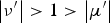 . Edwards et al. [17] have proved that −1 < k < 1 occurs if and only if SCs intersect USC. The four conditions are conditionally stable, and could oscillate under a certain matching network.
1) I-1. ν′ IS NEGATIVE AND μ′ IS POSITIVE
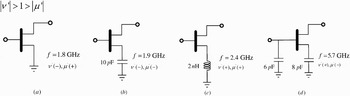
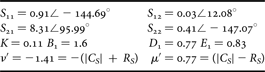
A two-port network containing only a single device as shown in Fig. 6(a) can generate the SC condition of Fig. 2(a). At f = 1.8 GHz, this two-port network has the state of ν′ = −1.41 and μ′ = 0.77. The stable region is outside SC (disk complement, ν′ < 0) and the origin of USC is included in the stable region (μ′ > 0). Like most practical microwave transistors, this case is potentially unstable and coincides with the factors of K and B 1 (K < 1: potential unstable cases [Reference Gonzalez6, Reference Vendelin, Pavio and Rohde10]). On collocating with the factor of D1, the unstable region occupied by SC can be estimated from the maximum and minimum distance between SC and the origin of USC, so as to initially evaluate the percentage of the available-matching region.
Schematics of two-port networks when |ν′| > 1 > |μ′|. (a) ν′ < 0, μ′ > 0. (b) ν′ < 0, μ′ < 0. (c) ν′ > 0, μ′ > 0. (d) ν′ > 0, μ′ < 0 (tick marks indicate the stable region).

2) I-2. ν′ IS NEGATIVE AND μ′ IS NEGATIVE
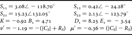
A device with a series-connected capacitor of 10 pF between source and ground is illustrated in Fig. 6(b), and the 1.9 GHz corresponding SC is plotted in Fig. 2(b). This capacitor enlarges the values of |S 11| and |S 22|, and then increases the possibility of oscillation [Reference Gonzalez6]. The difference between Figs 2(a) and 2(b) is that the stable region in Fig. 2(b) excludes the origin of USC because μ′ = −0.36 < 0. ν′ < 0 and μ′ < 0 imply a negative value of K from −1 to 0. It is conditionally stable.
3) I-3. ν′ IS POSITIVE AND μ′ IS POSITIVE
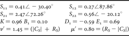
Figure 6(c) shows another two-port network with source-degeneration inductance. The 2.4 GHz SC in the ΓS plane is similar to the condition of Fig. 2(c). ν′ > 0 and μ′ > 0 mean that the stable region is inside SC (disk) and USC origin is in the stable region. The series feedback inductor of 2 nH makes the two-port network more stable. This topology has been commonly used in LNA design to achieve low noise figure and good input return loss simultaneously.
4) I-4. ν′ IS POSITIVE AND μ′ IS NEGATIVE
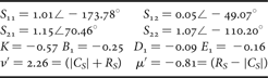
In this special case, a shunt capacitor of 6 pF is added at the input of a transistor, which has a series feedback capacitor of 8 pF at the source. SC in the ΓS plane at 5.7 GHz is illustrated in Fig. 2(d). The operating behavior of this two-port network is similar to that of Fig. 6(b) because most of the region in USC is unstable and the origin of USC is outside the stable region. However, they can be further differentiated by the new derived parameter, ν′. In this case, the stable region is inside SC (ν′ > 0).
B) Case II: 1 > |ν′| > |μ′| (conditionally stable)
SC in the ΓS plane is situated entirely inside USC for the case of 1 > |ν′| > |μ′|. These four situations are all conditionally stable with |K| > 1, and oscillation could occur under some matching networks.
1) II-1. ν′ IS NEGATIVE AND μ′ IS POSITIVE
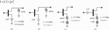
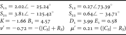
A two-port network containing a transistor with a series feedback capacitor of 4 pF and a shunt resistor of 80 Ω at the output is shown in Fig. 7(a). SC in the ΓS plane is plotted in Fig 3(a). Because ν′ < 0, the stable region is located outside SC. The shunt resistor allows the diameter of the SC to shrink obviously, and this phenomenon can be observed by the difference in the absolute values of ν′ and μ′. Compared with I-2, a resistor shunted at output can increase the stability of the two-port network.
Schematics of two-port networks when 1 > |ν′| > |μ′|. (a) ν′ < 0, μ′ > 0. (b) ν′ < 0, μ′ < 0. (c) ν′ > 0, μ′ > 0. (d) ν′ > 0, μ′ < 0 (tick marks indicate the stable region).

2) II-2. ν′ IS NEGATIVE AND μ′ IS NEGATIVE
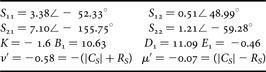
SC in the ΓS plane, which corresponds to the two-port network of Fig. 7(b) at 2.4 GHz, is plotted in Fig. 3(b). This circuit topology is the same as the previous example. In fact, the diameter of SC gradually increases due to the growing capacitive effect at higher operating frequency. The diameter of the unstable region expands from 0.51 (II-1) to 0.65 (this example). Finally, this network becomes more unstable at f = 2.4 GHz.
3) II-3. ν′ IS POSITIVE AND μ′ IS POSITIVE
A two-port network of Fig. 7(c) originates fromthe topology of Fig. 6(c). In this case, a negative resistance added in the source is equivalent to a positive feedback in the two-port network. When the resistance becomes more negative, the stable area inside SC is entirely shrunk. The relation between SC and USC is illustrated in Fig. 3(c).
4) II-4. ν′ IS POSITIVE AND μ′ IS NEGATIVE
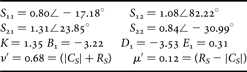
After adding a series capacitor at the input of Fig. 7(c), the topology of Fig. 7(d) results in μ′ = −0.08 < 0. From Equations (15) and (17), we can directly determine that USC origin is out of the stable region and SC is inside USC by values of ν′ and μ′. The stable region becomes smaller when compared with II-3.
From the above examples of Section II, the absolute values of μ′ and ν′ can reveal variations between stable and unstable regions (the diameter of SC).
C) Case III: |ν′| > |μ′| > 1 (unconditionally stable and absolutely unstable)
SC in the S plane is outside USC for the case of |ν′| > |μ′| > 1. Two situations are unconditionally stable and the other two situations are absolutely unstable. The corresponding networks for these situations are illustrated here.
1) III-1. ν′ IS NEGATIVE AND μ′ IS POSITIVE
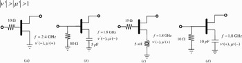
As illustrated in Fig. 8(a), it is a simple and effective approach to stabilize a potentially unstable amplifier by connecting in series a 10 Ω resistor at the input of the single transistor. However, the method suffers from gain reduction. Compared with I.1, the increasing μ′ implies that the point of SC closest to USC origin is gradually removed from the edge of USC. At the same time, the negative ν′ determines that all kinds of 2.4 GHz passive matching networks designed in the ΓS plane are unconditionally stable.
Schematics of two-port networks when |ν′| > |μ′| > 1. (a) ν′ < 0, μ′ > 0. (b) ν′ < 0, μ′ < 0. (c) ν′ > 0, μ′ > 0. (d) ν′ > 0, μ′ < 0 (tick marks indicate the stable region).

2) III-2. ν′ IS NEGATIVE AND μ′ IS NEGATIVE
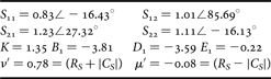
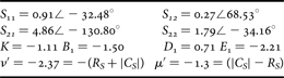
A two-port network with a series feedback capacitor of 5 pF at the transistor source and a shunt resistor of 80 Ω at the input is shown in Fig. 8(b). The capacitor could make the two-port network unstable. SC completely encloses USC and the stable region is outside SC in Fig. 4(b) because ν′ = −2.37 < 0. It is clear that an absolutely unstable situation occurs and any passive matching network in the ΓS plane results in |ΓOUT| > 1. The circuit is absolutely unstable.
3) III-3. ν′ IS POSITIVE AND μ′ IS POSITIVE
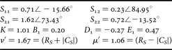
A two-port network containing a common source amplifier with a source degenerated inductor and an additional 15 Ω series resistor at f = 1.8 GHz is illustrated in Fig. 8(c). SC in the ΓS plane encloses USC completely, and the stable region is inside SC because ν′ = 1.67 > 0. SC of Fig. 4(c) looks very different from that of Fig. 4(a) even though both circuits have K > 1 and B 1 > 0. Thus, the parameter helps determine the relation between SC and USC.
4) III-4. ν′ IS POSITIVE AND μ′ IS NEGATIVE
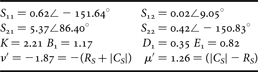
The circuit topology of Fig. 8(d) is identical to that of Fig. 8(b). From ν′ > 1 and μ′ < 1, SC is completely outside USC and the region inside SC is stable, as shown in Fig. 4(d). Obviously, the circuit is absolutely unstable. The S parameters and stability factors at 1.8 GHz are as follows:
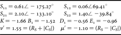
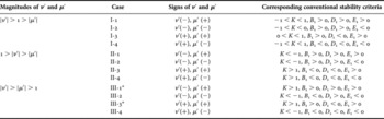
Table 1 compares the two geometrically derived parameters and the corresponding conventional stability factors (K, B 1, D 1, and E 1) for each geometrical situation. The signs of ν′ and μ′ are independent and useful in identifying each geometrical situation. However, the signs of K, B 1, D 1, and E 1 are dependent and lack geometrical meaning.
The comparison of stability parameters

* Unconditional stable.
V. DISCUSSIONS AND CONCLUSIONS
The complete analysis of stability is an important step in designing an active two-port network. Most discussions about stability in the literature [Reference Woods1, Reference Edwards and Sinsky5] only focus on the unconditionally stable case. There exist other conditions between SC and USC, and this paper has extended the criterion of stability to more situations by two derived parameters, μ′ and ν′.
A picture is worth a thousand words. Two stability parameters, μ′ and ν′, using the geometrical approach to assess the stability problem for a two-port network are established. Both magnitude and signs of them have distinct geometrical meanings in the ΓS plane, and 12 geometrical situations between SC and USC are classified. Simultaneously, practical two-port networks are also given to demonstrate the 12 conditions. This work provides a straightforward insight into the stability analysis of a two-port network and is helpful for the RF circuit design.
APPENDIX
The following is a bilinear transformation between the ω and z planes:

Let the radius of the circle be one in the ω plane. The following expression is to map the unit disk in the ω plane into a disk or a disk complement in the z plane:

which can be expanded as

If  , Equation (A.3) becomes

On the other hand, if  , Equation (A.3) becomes

This is equivalent to saying that the unit disk in the ω plane (|ω| < 1) maps into a disk in the z plane if  or into a disk complement in the z plane if
 . A bilinear transformation exists between the load and input reflection coefficients of a two-port network as shown below:
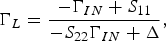
where

The radius and center of the relation in the ΓIN plane is
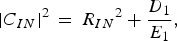
where

The condition,  , means that the mapped region of |ΓL| < 1 is an inner disk on the ΓIN plane. A bilinear transformation also exists between the output and source reflection coefficients of a two-port network as shown below:
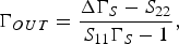
where

Also, the radius and center of the relation in the ΓS plane is
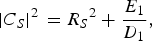
where

The condition is  to imply D1 < 0 for the mapping of |ΓOUT| < 1 on the ΓS plane being disk.
 Chin-Chun Meng received the B.S. degree in electrical engineering from National Taiwan University, Taipei, Taiwan, R.O.C., in 1985 and the Ph.D. degree in electrical engineering from University of California, Los Angeles, in 1992. He is now a full professor in the Department of Communication Engineering at National Chiao Tung University, HsinChu, Taiwan. His current research interests are in the areas of RFIC, microwave and millimeter-wave integrated circuits.
 Hung-Ju Wei received the B.S. degree from the Department of Electrical Engineering, National Center University, ChungLi, Taiwan, in 2003 and the M.S. degree from the Department of Microelectronics Engineering, National Cheng Kung University, Tainan, Taiwan, in 2005. He is currently working toward the Ph.D. degree at the Department of Communication Engineering, National Chiao Tung University, Hsinchu, Taiwan, R.O.C.. His research interests include high-frequency and analog integrated circuits designs.
Po-Hsing Sun received the B.S. degree from Chung Cheng Institute of Technology, Taoyuan, Taiwan, R.O.C., and M.S. degree from the Department of Electrical Engineering, National Chung-Hsing University, Taichung, Taiwan, R.O.C., in 2002. He is working at Chung-Shan Institute of Science and Technology (CSIST), and his current research focuses on the area of RFICs.