
 m=1,2
 m=3







1. Introduction
History-dependent random sequences are sequences in which the distribution of the outcome of the nth step depends non-trivially on the entire history of the process. Such sequences have numerous applications in sciences such as in polymer physics, where basic models of confined polymer chains in small enclosures consist of lattice sites which are occupied sequentially. The points evolve according to a self-avoiding random walk [Reference Domb8, Reference Freed9, Reference MacDonald, Joseph, Hunter, Moseley, Jan and Guttmann15], and investigation of the analytical properties of such processes remains an active area of research [Reference Benito, Karayiannis and Laso4, Reference Parreño, Ramos, Karayiannis and Laso16].
The focus of this paper is the so-called Ulam–Kac adder, following the ‘Ulam–Kac process’ defined in [Reference Clifford and Stirzaker7]. Let
 $\{U(n)\}_{n \geq 0}$
be a sequence of independent random variables such that U(n) is distributed uniformly on
 $\{0, 1, 2, \dots, n\}$
. The Ulam–Kac adder is the history-dependent random sequence defined by
 \begin{equation} X_{n + 1} = X_{n} + X_{U(n)}, \quad X_0 = 1.\end{equation}
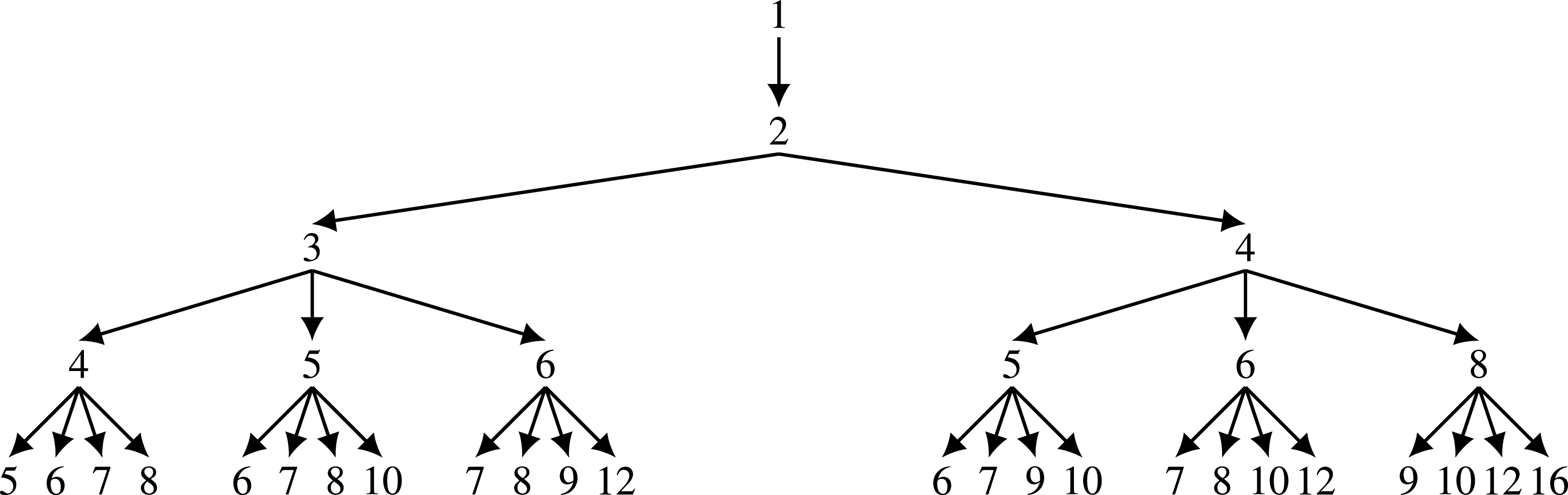
This sequence was first investigated by Ulam [Reference Ulam24]. The path space for the first five steps of this sequence is shown in Figure 1.
Illustration of the paths through the Ulam–Kac adder for the first five steps. Each of the paths is realized with equal probability.

The first explicit results on the behavior of the sequence were obtained by Kac [Reference Kac11], where it was shown, using generating functions and the method of steepest descent, that
 \begin{align} \log \mathbb{E}[X_n] &\sim 2 \sqrt{n}, \ \quad \qquad \quad \\[-22pt] \nonumber \end{align}
 \begin{align} \log \mathbb{E}[X_n^2] &\sim \sqrt{2 n \big(5 + \sqrt{17}\big)}, \end{align}
where we write
 $f(n) \sim g(n)$
if
 $\lim_{n \to \infty} f(n)/g(n) = 1$
. In [Reference Krasikov, Rodgers and Tripp14], (1.1) is generalized to
 \begin{equation} X_{n + 1} = X_{n} + \gamma X_{U(n)}, \quad X_0 = 1,\end{equation}
and the analogues of (1.2) and (1.3) are obtained. The Ulam–Kac adder was also considered in [Reference Ben-Naim and Krapivsky2] in the context of extensions of random Fibonacci sequences. There, the following results are conjectured based on numerical evidence.
Conjecture 1.1. There is an increasing sequence of positive constants
 $(c_m)_{m \geq 1}$
such that
 $\log \mathbb{E}[X_n^m] \sim c_m \sqrt{n}$
for all
 $m \geq 1$
.
Conjecture 1.2. There are positive constants
 $\mu, \sigma$
such that
 \begin{equation*} \frac{\log X_n - \mu n^{1/2}}{\sigma n^{1/4}} \to \mathcal{N}(0, 1) \text{ in law}. \end{equation*}
In [Reference Clifford and Stirzaker7], a Poisson-regularized continuous-time analogue of the Ulam–Kac adder was introduced as an alternate method of analyzing the asymptotic behavior of moments. This was applied to the first and second moments in several generalizations, and also in [Reference Roitershtein and Zhou18] to analyze the tail distribution of related sequences.
We note a structural similarity between (1.1) and elephant random walks [Reference Schütz and Trimper21, Reference Gut and Stadtmüller10]. There, with probability p (resp.
 $1 - p$
), a uniformly randomly chosen past increment is added (resp. subtracted) to the current state. In the Ulam–Kac adder, we add a randomly chosen past position rather than a past increment. Since positions are cumulative sums of increments, the Ulam–Kac adder can be viewed as an integrated analogue of the elephant random walk, which accounts for its much faster growth.
We also mention here a connection between the Ulam–Kac adder and addition chains which does not appear to have been explicitly stated previously. An addition chain for n is a sequence
 $(a_0, a_1, a_2, \dots, a_{m - 1}, a_m)$
such that
 $a_0 = 1$
and
 $a_m = n$
, where
 $a_{i} = a_{j} + a_{k}$
for each
 $1 \leq i \leq m$
and some
 $0 \leq j, k < i$
. An open problem in computer science is to efficiently obtain the shortest addition chain for arbitrary n [Reference Brauer6, Reference Scholz19, Reference Schönhage20, Reference Stolarsky22]. This remains an active area of research in high-performance computing [Reference Bahig and Kotb1, Reference Kadir, Mohamed, Mohamad, Mamat and Muhammed12]. In the case
 $j = i - 1$
, the chain is said to have taken a star step. With reference to Figure 1, we note that each realization of the Ulam–Kac adder is an addition chain consisting only of star steps. Such chains are called Brauer chains, or simply star chains. Computing
 $\mathbb{P}(X_k = n)$
is equivalent to computing the number of Brauer chains for n that have length k. The first-passage times of the Ulam–Kac adder are therefore directly related to minimal-length Brauer chains.
The main result of this paper is Theorem 1.1, which provides an affirmative answer to Conjecture 1.1 as well as bounds on the constants
 $c_m$
appearing therein.
Theorem 1.1 (Main result.) For all
 $m \geq 1$
, there exists a
 $c_m \in [2m, 2^{(m+3)/2} (m/{\mathrm{e}})^{m/2}{\mathrm{e}}^{3 \sqrt{m}}]$
such that
 \begin{equation} \log \mathbb{E}[X_n^m] \sim c_m \sqrt{n} . \end{equation}
We note that for a given m, high-accuracy numerical approximations of
 $c_m$
can be obtained as explained in Remark 5.1, although no formula for a generic m exists. The remainder of this paper is organized as follows. In Section 2, we provide a brief review of the basic method of computation for the
 $m = 1, 2$
moments. Then, Section 3 contains our outline of the main steps of the proof. In Section 4 we apply our main result to compute
 $\mathbb{E}[X_n^3]$
explicitly and compare its value to a previous numerical estimation. Section 5 contains all the proofs of the intermediate results required to obtain the main theorem. Finally, Section 6 contains our remarks on the tightness of the bounds in the main result, as well as some additional conjectures related to this work.
2. The
 $m = 1, 2$
moments

The basic method for the analysis of the Ulam–Kac adder is to condition on possible values of U(n) and telescope the resulting series [Reference Kac11], which we will now demonstrate. Defining
 $\mu_n \ :\!= \, \mathbb{E}[X_n]$
, (1.1) gives
 \begin{equation} \mu_{n + 1} = \mu_{n} + \mathbb{E}[X_{U(n)}] = \mu_{n} + \frac{1}{n + 1}\sum_{\ell = 0}^{n} \mu_{\ell},\end{equation}
where we have applied
 $\mathbb{E}[X_{U(n)} \,|\, U(n) = \ell] = \mu_{\ell}$
. We then take
 $n \to n + 1$
in (2.1) and eliminate the remaining sum to obtain
 \begin{align} \mu_{n + 2} &= \mu_{n +1 } + \frac{1}{n + 2}\Bigg[\mu_{n+1} + \sum_{m = 0}^{n} \mu_{m}\Bigg], \nonumber \\[3pt] 0 &= (n + 2) \mu_{n + 2} - 2 (n + 2) \mu_{n + 1} + (n + 1) \mu_{n}, \end{align}
along with the initial conditions
 $\mu_{0} = 1$
,
 $\mu_{1} = 2$
. The classical Laguerre polynomials
 $L_n(x)$
satisfy the recurrence relation [Reference Szegő23]
 \begin{equation*} (2 + k)L_{k + 2}(x) - (2k + 3 - x) L_{k + 1}(x) + (k + 1) L_{k}(x) = 0, \qquad L_{0} = 1,\ L_{1} = 1 - x.\end{equation*}
Comparing this to (2.2), we see that they coincide when
 $x = -1$
and therefore
 \begin{equation*} \mu_n = L_{n}(\!-1) = \sum_{\ell = 0}^{n} \binom{n}{\ell} \frac{1}{\ell!}.\end{equation*}
This directly leads to
 $\log \mu_n \sim 2 \sqrt{n}$
using the known asymptotics of Laguerre polynomials. See [Reference Ben-Naim and Krapivsky2, Reference Krasikov, Rodgers and Tripp14] for alternative calculations of the same result. We note that the generalization (1.4) results in the family of Laguerre polynomials
 $\mu_n = L_n(\!-\gamma)$
.
We will now compute the second moment of the Ulam–Kac adder
 $\sigma_n \ :\!= \, \mathbb{E}[X_n^2] $
by determining an ordinary differential equation (ODE) satisfied by the generating function of the sequence
 $\{\sigma_n\}_{n \geq 0}$
. By squaring (1.1), we obtain
 \begin{equation} X_{n + 1}^2 = X_{n}^2 + 2 X_{n} X_{U(n)} + X_{U(n)}^2 .\end{equation}
We would like to calculate the expected value of this equation, but the cross term
 $X_{n} X_{U(n)}$
is not easily identified with
 $\sigma_n$
. To obtain a closed system of recurrence relations, we define
 $\alpha_n \ :\!= \, \sum_{\ell = 0}^{n-1} \mathbb{E}[X_{n} X_{\ell}]$
; then, taking the expectation of (2.3) gives
 \begin{equation} \sigma_{n + 1} = \sigma_{n} + \frac{2}{n + 1} (\sigma_n + \alpha_n) + \frac{1}{n + 1} \sum_{\ell = 0}^{n} \sigma_{\ell}. \end{equation}
Furthermore, by applying (1.1) to
 $\alpha_{n + 1}$
, we obtain
 \begin{equation}\alpha_{n +1} = \sigma_{n} + \alpha_n + \frac{1}{n + 1} \sum_{\ell = 0}^{n} (\sigma_\ell + 2 \alpha_\ell). \end{equation}
We define the generating functions
 $G(z) = \sum_{n = 0}^{\infty} \sigma_n z^n$
and
 $M(z) = \sum_{n = 0}^{\infty} \alpha_n z^n$
, which have radii of convergence equal to 1, as will be shown in Section 3. Multiplying (2.4) and (2.5) through by
 $(n + 1) z^n$
and summing the resulting expressions over
 $n \geq 0$
gives
 \begin{alignat*}{2} G' & = (z G)' + 2(G + M) + \frac{1}{1 - z} G, & G(0) & = 1 \\[3pt] M' & = (z G)' + (z M)' + \frac{1}{1 - z}(G + 2M), \quad & M(0) & = 0.\end{alignat*}
We can eliminate M(z) using the first of these equations to obtain
 \begin{equation*} (z^2 - 6z + 7) G(z) + (3z - 8) (1 - z)^2 G'(z) + (1 - z)^4 G''(z) = 0, \quad G(0) = 1,\ G'(0) = 4,\end{equation*}
which is the ODE we sought. Substitution of the asymptotic form
 ${\mathrm{e}}^{S(x)}$
into here and application of the method of dominant balance [Reference Bender and Orszag3] informally provides
 $\log \sigma_n \sim \sqrt{2(5 + \sqrt{17}) n}$
, which can be made fully rigorous with Theorem 1.1.
3. Outline of proof
We will begin by constructing a closed set of recurrence relations for the mth moment. Then, we will create the system of linear differential equations for the associated generating functions. By closely studying the properties of the matrices defining this system, we are able to apply certain technical results for the asymptotic behavior of their solutions and thereby obtain Theorem 1.1.
Let
 $\mathcal{M}_{\geq 1}$
be the set which contains the empty set
 $\varnothing$
plus all non-empty ordered multisets of finite cardinality on positive integers. We write an element
 $\mathfrak{a} \in \mathcal{M}_{\geq 1}$
as
 $\mathfrak{a} = [p_1, p_2, p_3, \dots, p_n]$
, where
 $p_i \in \mathbb{Z}_{\geq 1}$
for all
 $1 \leq i \leq n$
and
 $p_i \geq p_j$
for
 $i < j$
. We call each
 $p_i$
a part of
 $\mathfrak{a}$
and write
 $| \mathfrak{a} | = n$
when
 $\mathfrak{a}$
has n parts. We reserve
 $\lVert \mathfrak{a} \rVert$
to denote the sum of all parts of
 $\mathfrak{a}$
. We write
 $\mathfrak{a} = \mathfrak{b}$
for two non-empty elements
 $\mathfrak{a}, \mathfrak{b} \in \mathcal{M}_{\geq 1}$
if and only if both
 $| \mathfrak{a} | = | \mathfrak{b} |$
and
 $p_i$
of
 $\mathfrak{a}$
is equal to
 $p_i$
of
 $\mathfrak{b}$
for all
 $1\leq i \leq | \mathfrak{a} | $
. Each non-empty element
 $\mathfrak{a} \in \mathcal{M}_{\geq 1}$
has
 $2^{| \mathfrak{a} |}$
multisubsets
 $\mathfrak{c} \subseteq \mathfrak{a}$
formed by the power set of parts of
 $\mathfrak{a}$
arranged in descending order. For example,
 $\mathfrak{a} = [2, 1, 1]$
has the multisubsets
 $\{\varnothing, [2], [1], [1], [2, 1], [2, 1], [1, 1], [2, 1, 1] \}$
.
We also recall that addition and subtraction can be defined on multisets as follows. If
 $\mathfrak{a}, \mathfrak{b} \in \mathcal{M}_{\geq 1}$
where
 $| \mathfrak{a} | = m$
and
 $| \mathfrak{b} | = n$
then
 $\mathfrak{a} + \mathfrak{b}$
is the multiset with
 $m + n$
parts created from the disjoint union of all parts of
 $\mathfrak{a}$
and
 $\mathfrak{b}$
arranged in descending order. The subtraction
 $\mathfrak{a} - \mathfrak{b}$
, defined if
 $\mathfrak{b} \subseteq \mathfrak{a}$
, is equal to any multisubset
 $\mathfrak{c} \subseteq \mathfrak{a}$
such that
 $\mathfrak{c} + \mathfrak{b} = \mathfrak{a}$
. Successive addition and subtraction should be applied from left to right, e.g. we have
 $\mathfrak{a} + \mathfrak{b} - \mathfrak{c} = (\mathfrak{a} + \mathfrak{b}) - \mathfrak{c}$
.
Let
 $\mathcal{P}(n) = \{\mathfrak{p} \in \mathcal{M}_{\geq 1} \colon \lVert \mathfrak{p} \rVert = n \}$
be the set of all integer partitions of
 $n\geq 0$
with the definition
 $\mathcal{P}(0) = \{\varnothing\}$
. We define
 $\mathcal{C}^{(m)}$
as the set of all terms that can occur in our system of recurrence relations for the mth moment,
 \begin{equation*} \mathcal{C}^{(m)} = \{ C_{n}^{(m)}(q; \, \mathfrak{p}) \colon n \geq 1, 1 \leq q \leq m, \mathfrak{p} \in \mathcal{P}(m - q) \}, \quad m \geq 1,\end{equation*}
such that each element of
 $\mathcal{C}^{(m)}$
is given by
 \begin{equation} C_n^{(m)}(q; \, \mathfrak{p}) = \sum_{\alpha_1 = 0}^{n - 1} \sum_{\alpha_2 = 0}^{n - 1} \cdots \sum_{\alpha_{| \mathfrak{p} |} = 0}^{n - 1} \mathbb{E}\Bigg[X_n^q \prod_{\ell = 1}^{| \mathfrak{p} |} X^{p_\ell}_{\alpha_\ell} \Bigg].\end{equation}
We note the initial-value convention at
 $n = 0$
that an empty product equals 1 and an empty sum equals 0 such that
 $C_0^{(m)}(q; \, \mathfrak{p}) = 0$
whenever
 $| \mathfrak{p} | \geq 1$
, while
 $C_0^{(m)}(m; \, \varnothing) = \mathbb{E}[X_0^m] = 1$
.
Motivated by the patterns observed in (2.4) and (2.5), we generally expect to obtain recurrence relations each with three types of terms:
 $x_n$
,
 $x_n/(n + 1)$
, and
 $({1}/({n+1}))\sum_{\ell = 0}^{n} x_\ell$
. We therefore introduce the following notation:
 \begin{equation} \hat{x}_{n} \ :\!= \, \frac{x_n}{n + 1}, \qquad \overline{x}_{n} \ :\!= \, \frac{1}{n + 1} \sum_{\ell = 0}^{n} x_{\ell}.\end{equation}
Putting
 $X(z) = \sum_{n = 0}^{\infty} x_n z^n$
wherever X(z) is defined, we note that
 \begin{equation} \sum_{n = 0}^{\infty} (n + 1) x_n z^n = \frac{\text{d}}{\text{d} z} [z X(z)], \qquad \sum_{n = 0}^{\infty} (n + 1) \hat{x}_n z^n = X(z), \qquad \sum_{n = 0}^{\infty} (n + 1) \overline{x}_n z^n = \frac{X(z)}{1 - z}.\end{equation}
We can now compute the most general recurrence relation, which is the result of the following lemma whose proof can be found in Section 5.1.
Lemma 3.1. For a fixed
 $m \geq 1$
, each
 $C_{n+1}^{(m)}(q; \, \mathfrak{p}) \in \mathcal{C}^{(m)}$
satisfies
 \begin{align} C_{n + 1}^{(m)}(q; \, \mathfrak{p}) &= \sum_{\mathfrak{b} \subseteq \mathfrak{p}} C_{n}^{(m)} (q + \lVert \mathfrak{b} \rVert ; \, \mathfrak{p} - \mathfrak{b}) \quad\quad\quad\qquad\qquad\qquad\qquad\qquad \\[-35pt] \nonumber \end{align}
 \begin{align} &\quad \ + \sum_{\beta = 1}^{q - 1} \binom{q}{\beta} \sum_{\mathfrak{b} \subseteq \mathfrak{p} + [q - \beta ]} \hat{C}_{n}^{(m)} (\beta + \lVert \mathfrak{b} \rVert ; \, \mathfrak{p}+ [q - \beta ] - \mathfrak{b}) \\[-35pt] \nonumber \end{align}
 \begin{align} &+ \sum_{\substack{\mathfrak{b} \subseteq \mathfrak{p} + [q ] \\[3pt] \mathfrak{b} \neq \varnothing}} \overline{C}_{n}^{(m)} (\lVert \mathfrak{b} \rVert ; \, \mathfrak{p}+ [q ] - \mathfrak{b}). \quad \qquad \qquad \qquad \end{align}
We will show how (3.4) can be written as a finite linear system of first-order difference equations. This will allow us to obtain preliminary results concerning the asymptotic behavior of the system. We first collect the
 $C_{n}^{(m)}(q; \, \mathfrak{p})$
into a vector,
 $c^{(m)}_n$
. The following definition is important for this construction. For a fixed
 $m \geq 1$
, the vector
 $c^{(m)}_n = ( C_{n}^{(m)}(q; \, \mathfrak{p}) )$
is said to be in canonical ordering if its entries are sorted first by descending q, then by ascending
 $| \mathfrak{p} |$
. The number of entries in this vector is
 $\mathfrak{C}(m)$
.
Now, (3.4) can first be expressed generically as
 \begin{equation} c^{(m)}_{n + 1} = \mathbf{C}_1 c^{(m)}_{n} + \frac{1}{n + 1}\mathbf{C}_2 c^{(m)}_{n } + \frac{1}{n + 1} \sum_{\ell = 0}^{n} \mathbf{C}_3 c^{(m)}_{\ell}.\end{equation}
Each of the matrices
 $\mathbf{C}_1$
,
 $\mathbf{C}_2$
, and
 $\mathbf{C}_3$
have entries which depend only on m and can be extracted from (3.4a), (3.4b), and (3.4c), respectively. Define
 \begin{equation*} d^{(m)}_{n + 1} = \sum_{\ell = 0}^{n} \mathbf{C}_3 c^{(m)}_{\ell} = \mathbf{C}_3 c^{(m)}_{n} + d^{(m)}_{n}.\end{equation*}
Then, we have
 \begin{equation} \begin{pmatrix} c^{(m)}_{n + 1} \\[3pt] d^{(m)}_{n + 1} \end{pmatrix} = \begin{pmatrix} \mathbf{C}_1 + \dfrac{1}{n + 1}( \mathbf{C}_2 + \mathbf{C}_3 ) &\quad \dfrac{1}{n + 1} \mathbf{I} \\[3mm] \mathbf{C}_3 & \mathbf{I} \end{pmatrix} \begin{pmatrix} c^{(m)}_{n} \\[3pt] d^{(m)}_{n} \end{pmatrix}.\end{equation}
We can now apply the following result due to Pituk on asymptotically constant systems of linear difference equations.
Theorem 3.1 ([Reference Pituk17, Theorem 1].) Let
 $x = (x_n)_{n \in \mathbb{N}}$
be a solution of the difference equation
 $x_{n + 1} = \mathbf{L}_n x_n$
,
 $n \in \mathbb{N}$
. If
 $\lim_{n \to \infty} \mathbf{L}_n = \mathbf{L}$
for a constant matrix
 $\mathbf{L}$
, then either
 $x_n = 0$
for all large n or the limit
 $\rho(x) = \lim_{n \to \infty} ||x_n||^{1/n}$
exists and is equal to the modulus of one of the eigenvalues of
 $\mathbf{L}$
.
Examining (3.6), Theorem 3.1 applies with
 \begin{equation} \mathbf{L} = \begin{pmatrix} \mathbf{C}_1 &\quad \mathbf{0} \\[3pt] \mathbf{C}_3 &\quad \mathbf{I} \end{pmatrix}.\end{equation}
We require the following proposition to compute the eigenvalues of
 $\mathbf{L}$
.
Proposition 3.1. The matrix
 $\mathbf{C}_{\mathbf{1}}$
is lower triangular and each entry on its diagonal is 1.
Proof. The entries of
 $\mathbf{C}_1$
are controlled by (3.4a), which implies that
 $(q; \, \mathfrak{p})$
depends on each
 $(q + \lVert \mathfrak{b} \rVert; \, \mathfrak{p} - \mathfrak{b})$
for
 $\mathfrak{b} \subseteq \mathfrak{p}$
. Each
 $(q + \lVert \mathfrak{b} \rVert; \, \mathfrak{p} - \mathfrak{b})$
comes before
 $(q; \, \mathfrak{p})$
in the canonical ordering, which implies the lower triangular structure. There is a unique
 $\mathfrak{b}$
such that
 $(q + \lVert \mathfrak{b} \rVert; \, \mathfrak{p} - \mathfrak{b}) = (q; \, \mathfrak{p} )$
, namely the empty set, and hence there are ones on the diagonal of
 $\mathbf{C}_1$
.
By Proposition 3.1 and (3.7),
 $\mathbf{L}$
is a lower triangular matrix whose diagonal entries are all equal to 1, and hence
 $\mathbf{L}$
has one eigenvalue equal to 1 of multiplicity
 $2\mathfrak{C}(m)$
. Hence, by Theorem 3.1, each increasing solution
 $x_n$
of (3.6) satisfies
 $\lim_{n \to \infty} ||x_n||^{1/n} = 1$
. To each sequence
 $(C_{n}^{(m)}(q; \, \mathfrak{p}))_{n \geq 0}$
we associate a generating function
 $G^{(m)}_{q, \mathfrak{p}}(z)$
defined by
 \begin{equation} G^{(m)}_{q, \mathfrak{p}}(z) = \sum_{n = 0}^{\infty} C_{n}^{(m)}(q; \, \mathfrak{p}) z^n.\end{equation}
Pituk’s theorem gives
 $\lim_n \lVert c^{(m)}_n \rVert^{1/n} = 1$
and hence a radius of convergence of at least 1, while the lower bound
 $c_n^{(m)} \geq 1$
for
 $n \geq 1$
ensures that the coefficients do not decay geometrically, so the radius of convergence is at most (hence exactly) 1.
We will apply Lemma 3.1 to obtain a system of linear differential equations satisfied by these generating functions. Therefore, we collect them into a vector
 $g^{(m)}(z) = (G^{(m)}_{q, \mathfrak{p}}(z))$
in the canonical ordering—with reference to (3.5), this implies that
 \begin{equation} g^{(m)}(z) = \sum_{n = 0}^{\infty} c_{n}^{(m)} z^n,\end{equation}
where the equality is elementwise. We will sometimes write
 $(q; \, \mathfrak{p})$
instead of
 $G^{(m)}_{q, \mathfrak{p}}(z)$
for brevity. In that notation,
 $(q; \, \mathfrak{p})_i$
will refer to the ith generating function when listed in the canonical ordering (equivalently, the ith element of the vector
 $g^{(m)}(z)$
). Similarly,
 $\mathfrak{p}_i$
will refer to
 $\mathfrak{p}$
of
 $(q; \, \mathfrak{p})_i$
. The m label will generally be omitted for brevity except where required; note also that
 $m = q + \lVert \mathfrak{p} \rVert$
.
Now, we multiply each term in (3.5) by
 $(n + 1)z^n$
and sum the resulting equation over all
 $n \geq 0$
to transform the recurrence relations to differential equations. By applying (3.3) and (3.9), we obtain the system
 \begin{equation} g'(z) = z \mathbf{C}_1 g'(z) + \bigg[\mathbf{C}_1 + \mathbf{C}_2 + \frac{1}{1 - z} \mathbf{C}_3 \bigg] g(z).\end{equation}
The matrix
 $\mathbf{I} - z \mathbf{C}_1$
is invertible for
 $0 \leq z < 1$
(by Proposition 3.1), so we can write
 \begin{equation} g'(z) = \mathbf{R}\bigg(\frac{1}{1-z}\bigg)g(z), \qquad \mathbf{R}\bigg(\frac{1}{1-z}\bigg) = (\mathbf{I} - z \mathbf{C}_1)^{-1}\bigg[\mathbf{C}_1 + \mathbf{C}_2 + \frac{1}{1 - z}\mathbf{C}_3\bigg].\end{equation}
Letting
 $u = 1/(1 - z)$
, we make the substitution
 \begin{equation} g(z) = \mathbf{P}(u) h(u), \qquad \mathbf{P}(u) = \text{diag}\big\{u^{| \mathfrak{p}_{1} |}, u^{| \mathfrak{p}_{2} |}, \dots, u^{| \mathfrak{p}_{\mathfrak{C}(m)} |}\big\},\end{equation}
which transforms (3.11) to a new system,
 \begin{equation} h'(u) = \mathbf{S}(u) h(u).\end{equation}
In Section 5.2, we establish the following lemma which collects the relevant properties of
 $\mathbf{S}(u)$
.
Lemma 3.2. For
 $u \geq 1$
and for some
 $N \geq 1$
there is a sequence of matrices
 $\{\mathbf{M}_i\}_{0 \leq i \leq N}$
such that
 $\mathbf{M}_0$
is primitive with Perron–Frobenius eigenvalue
 $\lambda^{(m)} \leq 2^{m+1} (m/{\mathrm{e}})^m{\mathrm{e}}^{6 \sqrt{m}}$
and such that the matrix
 $\mathbf{S}(u)$
defined in (3.13) can be expressed as
 $\mathbf{S}(u) = \sum_{i = 0}^{N} u^{-i} \mathbf{M}_i$
.
We will obtain our main result using the Tauberian theorem of Kohlbecker [Reference Kohlbecker13] as quoted in [Reference Bingham, Goldie and Teugels5].
Theorem 3.2 ([Reference Bingham, Goldie and Teugels5, Theorem 4.12.1].) Let
 $\theta$
be a measure on
 $\mathbb{R}$
, supported by
 $[0,\infty)$
and finite on compact sets. Let
 $K(\rho) \ :\!= \, \int_{[0,\infty)} {\mathrm{e}}^{-x/\rho} \, {\mathrm{d}}\theta(x)$
 $(\rho > 0)$
. Let
 $\alpha > 1$
,
 $B > 0$
. Then
 \begin{equation} \log\!(\theta[0,x]) \sim B x^{1/\alpha} \quad (x \to \infty) \end{equation}
if and only if
 \begin{equation} \log\!(K(\rho)) \sim (\alpha - 1)(B/\alpha)^{\alpha/(\alpha - 1)} \rho^{1/(\alpha - 1)} \quad (\rho \to \infty).\end{equation}
We can now prove Theorem 1.1.
Proof of Theorem 1.1. Referring to (3.8), our goal is to study the asymptotic behavior of
 $G_{m, \varnothing}^{(m)}(z) = \sum_{n = 0}^{\infty} \mathbb{E}[X_n^m]z^n$
. In the notation of Theorem 3.2, we can define the measure
 $\theta^{(m)} = \sum_{n\geq0} \mathbb{E}[X_{n}^{m}] \delta_n$
and take
 $z = {\mathrm{e}}^{-1/\rho}$
for
 $z \in [0, 1)$
, giving
 $K(\rho(z)) = G_{m, \varnothing}^{(m)}(z)$
. Recalling that
 $u = 1/(1-z)$
and thus
 $u \to \infty$
, as
 $\rho \to \infty$
we have
 $\rho = -1/\log\!(z) = -1/\log\!(1 - u^{-1}) \sim u$
and therefore, if
 \begin{equation} \log G_{m, \varnothing}^{(m)}(z) \sim \lambda^{(m)} u, \end{equation}
then we identify
 $\alpha = 2$
and
 $B = 2 \sqrt{\lambda^{(m)}}$
in (3.15); (3.14) then implies that
 \begin{equation} \log \sum_{\alpha = 0}^{n} \mathbb{E}[X_\alpha^m] \sim 2 \sqrt{\lambda^{(m)}} \sqrt{n}. \end{equation}
By the monotonicity of
 $X_{\alpha}$
, we have
 $(n + 1)^{-1} \sum_{\alpha = 0}^{n} \mathbb{E}[X_\alpha^m] \leq \mathbb{E}[X_n^m] \leq \sum_{\alpha = 0}^{n} \mathbb{E}[X_\alpha^m]$
which, upon taking logarithms, multiplying through by
 $n^{-1/2}$
, taking
 $n \to \infty$
, and applying (3.17), gives
 $\log \mathbb{E}[X_n^m] \sim 2 \sqrt{\lambda^{(m)}} \sqrt{n}$
, which implies (1.5) by taking
 $c_m = 2 \sqrt{\lambda^{(m)}}$
. Therefore, to complete the proof it remains to establish (3.16).
By Lemma 3.2, we can express (3.13) as
 \begin{equation} h'(u) = (\mathbf{A} + \mathbf{B}(u)) h(u), \end{equation}
where
 $\mathbf{A}$
is primitive and
 $\lVert \mathbf{B}(u)\rVert \leq \mathbf{B}^\star/u$
for
 $u \geq 1$
and some non-negative
 $\mathbf{B}^\star$
. We will repeatedly use the fact that, for the solution of interest to (3.18), we have
 $h(u) \geq 0$
for
 $u \geq 1$
and
 $h(u) > 0$
componentwise for
 $u > 1$
, since by (3.12) and (3.9) each component of h(u) is a positive multiple of a generating function evaluated at
 $z(u) \in [0, 1)$
whose coefficients
 $(c^{(m)}_n)_i$
are non-negative, and positive for
 $n \geq 1$
. Let
 $w >0$
be the left Perron–Frobenius eigenvector of
 $\mathbf{A}$
, i.e.
 $w^{\top}\mathbf{A} = \lambda w^{\top}$
. Define
 $\phi(u) \ :\!= \, w^{\top} h(u) > 0$
, where positivity at
 $u = 1$
follows from
 $h_1(1) = G^{(m)}_{m, \varnothing}(0) = \mathbb{E}[X_0^m] = 1$
, and note that
 $\lVert h(u) \rVert_1 \leq \phi(u)/\min_i w_i$
. Multiplying (3.18) from the left by
 $w^{\top}$
gives
 $\phi'(u) = \lambda \phi(u) + w^{\top} \mathbf{B}(u) h(u)$
. But then
 $\lVert w^{\top} \mathbf{B}(u) h(u) \rVert \leq \lVert w^{\top}\rVert \lVert \mathbf{B}^\star/u\rVert \lVert h(u) \rVert \leq b \phi(u)/u$
for some
 $b > 0$
. Therefore,
 \begin{equation*} (\lambda - b/u)\phi(u) \leq \phi'(u) \leq (\lambda + b/u)\phi(u) \implies \lambda - b/u \leq (\!\log \phi(u))' \leq \lambda + b/u, \end{equation*}
and integration on [1, u] gives
 $\log \phi(u) \sim \lambda u$
.
We must now establish that
 $\log\phi(u) \sim \lambda u \implies \log G_{m,\varnothing}^{(m)}(z) \sim \lambda u$
. By (3.12) and (3.9) and the definition of the canonical ordering,
 $h_1 = G_{m, \varnothing}^{(m)}(z)$
. We obtain the upper bound
 \begin{equation} \log \phi(u) > \log\!\big(w_1 G_{m, \varnothing}^{(m)}(z)\big) = \log G_{m, \varnothing}^{(m)}(z) + O(1). \end{equation}
We next obtain a lower bound. Since
 $u \geq 1$
, we have
 \begin{equation} \phi(u) = \sum_{i = 1}^{\mathfrak{C}(m)} w_i h_i(u) = \sum_{i = 1}^{\mathfrak{C}(m)} w_i u^{-|\mathfrak{p}_i|}g_i(z(u)) \leq \sum_{i = 1}^{\mathfrak{C}(m)} w_i g_i(z(u)) = \sum_{i = 1}^{\mathfrak{C}(m)} w_i \sum_{n = 0}^{\infty} \big(c_n^{(m)}\big)_i z(u)^n . \end{equation}
We can take
 $X_{\alpha_\ell}^{p_\ell} \leq X_{n}^{p_\ell}$
in (3.1) to obtain
 $C_{n}^{(m)}(q; \, \mathfrak{p}) \leq n^{|\mathfrak{p}|}C_{n}^{(m)}(m; \, \varnothing)$
or, in the canonical ordering,
 $\big(c_n^{(m)}\big)_i \leq n^{|\mathfrak{p}_i|}\big(c_n^{(m)}\big)_1 \leq n^{m}\big(c_n^{(m)}\big)_1$
. Substituting this into (3.20) and defining
 $w_c \ :\!= \, \sum_{i = 1}^{\mathfrak{C}(m)} w_i$
gives
 $\phi(u) \leq w_c \sum_{n = 0}^{\infty} n^m \big(c_n^{(m)}\big)_1 z(u)^n$
.
Let r be such that
 $0 < z < r < 1$
. Then
 \begin{equation*} \phi(u) \leq w_c \sum_{n = 0}^{\infty} [n^m (z/r)^{n}]\big(c_n^{(m)}\big)_1 r^n \leq w_c\bigg[\log\bigg(\frac{r}{z}\bigg)\bigg]^{-m} G_{m, \varnothing}^{(m)}(r) \end{equation*}
by maximizing
 $n^m (z/r)^{n} $
with respect to n and absorbing constants into
 $w_c$
. Since
 $z = 1 - u^{-1}$
we take
 $r = z(u + 1) = 1 - (u + 1)^{-1}$
, from which it follows that
 $1/\log\!(r/z) \leq u^2$
. Restricting to
 $u \geq 2$
(valid since we consider
 $u \to \infty$
), we have
 \begin{equation*} \phi(u) \leq w_c u^{2m} G_{m, \varnothing}^{(m)}(z(u + 1)) \implies \log \phi(u - 1) + O(\log\!(u)) < \log G_{m, \varnothing}^{(m)}(z(u)). \end{equation*}
Combining this with (3.19) gives, provided again that
 $u\geq 2$
,
 \begin{equation*} \log \phi(u - 1) + O(\!\log \!(u)) < \log G_{m, \varnothing}^{(m)}(z) < \log \phi(u) + O(1). \end{equation*}
Multiplying this through by
 $u^{-1}$
, taking
 $u \to \infty$
, and using
 $\log \phi(u) \sim \lambda u$
shows that
 $\log G_{m, \varnothing}^{(m)}(z)/u$
is squeezed by
 $\lambda$
, establishing (3.16).
Given
 $\log \mathbb{E}[X_n^m] \sim c_m \sqrt{n}$
, we place bounds on
 $c_m$
in the general case. From Jensen’s inequality, we have
 $\mathbb{E}[X_n^m] \geq \mathbb{E}[X_n]^m$
and so, by the results of Section 2,
 \begin{equation*} \log \mathbb{E}\big[X_n^m\big] \geq m \log \mathbb{E}[X_n] \sim 2m \sqrt{n}, \end{equation*}
which implies that
 $c_m \geq 2m$
. Since
 $c_m = 2 \sqrt{\lambda^{(m)}}$
, the upper bound in Theorem 1.1 immediately follows from the upper bound on
 $\lambda^{(m)}$
in Lemma 3.2. This completes the proof of the bounds on
 $c_m$
.
Finally, we establish the monotonic growth of the constants
 $c_m$
. For
 $m \geq 2$
, Lyapunov’s inequality gives
 $(\mathbb{E}[X_n^m])^{1/m} \geq (\mathbb{E}[X_n^{m-1}])^{1/(m-1)}$
. Taking logarithms, dividing by
 $\sqrt{n}$
, and passing to the limit gives
 $c_m/m \geq c_{m-1}/(m - 1)$
, or equivalently
 $c_m \geq ({m}/({m-1})) c_{m - 1} > c_{m - 1}$
since
 $c_{m - 1} > 0$
. This completes the proof of Theorem 1.1.
4. Example:
$m = 3$

We will now compute the exact value of the third moment of the Ulam–Kac adder,
 $\mathbb{E}[X_n^3]$
. This has not been explicitly computed previously, although [Reference Ben-Naim and Krapivsky2] estimated
 $\log \mathbb{E}[X_n^3] \sim 6.5 \sqrt{n}$
based on numerical evidence. When
 $m = 3$
, there are four types of sequences in
 $\mathcal{C}^{(3)}$
, namely
 \begin{align*} \gamma_n & \ :\!= \, C_{n}^{(3)}(3; \, \varnothing) = \mathbb{E}[X_n^3], \\[3pt] \tau_n & \ :\!= \, C_{n}^{(3)}(2; \, [1]) = \sum_{\ell = 0}^{n-1} \mathbb{E}[X_{n}^2 X_\ell], \\[3pt] \xi_n & \ :\!= \, C_{n}^{(3)}(1; \, [2]) = \sum_{\ell = 0}^{n-1} \mathbb{E}[X_{n} X_\ell^2], \\[3pt] \psi_n & \ :\!= \, C_{n}^{(3)}(1; \, [1,1]) = \sum_{\ell = 0}^{n-1}\sum_{k = 0}^{n-1} \mathbb{E}[X_{n} X_\ell X_k].\end{align*}
Applying Lemma 3.1, we obtain the following system of recurrence relations:
 \begin{align} \gamma_{n+1} & = \gamma_n + 3( 2 \hat{\gamma}_n + \hat{\tau}_n + \hat{\xi}_n) + \overline{\gamma}_n, \\[-10pt] \nonumber \end{align}
 \begin{align} \tau_{n + 1} & = \gamma_n + \tau_n + 2 (\hat{\gamma}_n + 2 \hat{\tau}_n + \hat{\psi}_n) + (\overline{\gamma}_n + \overline{\tau}_n + \overline{\xi}_n), \\[-10pt] \nonumber \end{align}
 \begin{align} \xi_{n + 1} & = \gamma_n + \xi_n + (\overline{\gamma}_n + \overline{\tau}_n + \overline{\xi}_n), \\[-10pt] \nonumber \end{align}
 \begin{align} \psi_{n + 1} & = \gamma_n + \psi_n + 2\tau_n + (\overline{\gamma}_n + 3 \overline{\tau}_n + 3 \overline{\psi}_n). \\[10pt] \nonumber \end{align}
We elaborate here on how (4.1b) is obtained; the other equations follow similarly. To calculate
 $\tau_{n + 1}$
we set
 $m = 3$
,
 $q = 2$
, and
 $\mathfrak{p} = [1]$
in (3.4). The set of multisubsets of
 $\mathfrak{p}$
is
 $\{[1],\varnothing \}$
, hence the term on the right-hand side of (3.4a) is
 $C_{n}^{(m)}(2 + 1; \, \varnothing) + C_{n}^{(m)}(2 + 0; \, [1]) = \gamma_n + \tau_n$
.
Consider now the term in (3.4b). Since
 $q = 2$
, the sum over
 $\beta$
contains only the term
 $\beta = 1$
, hence there will be an overall factor of
 $\binom{2}{1} = 2$
. The sum over
 $\mathfrak{b}$
is a sum over the four multisubsets of
 $\mathfrak{p} + [1] = [1, 1]$
, hence the entire term is
 \begin{equation*} 2[\hat{C}_{n}^{(m)} \big(1 + 2 ; \, \varnothing \big) + 2 \hat{C}_{n}^{(m)} (1 + 1 ; \, [1]) + \hat{C}_{n}^{(m)} (1 + 0 ; \, [1, 1])] = 2(\hat{\gamma}_n + 2\hat{\tau}_{n} + \hat{\psi}_{n}).\end{equation*}
Finally, the term in (3.4c) is a sum over the three non-empty multisubsets of
 $\mathfrak{p} + [2] = [2, 1]$
, giving
 \begin{equation} \overline{C}_{n}^{(m)} (3 ; \, \varnothing) + \overline{C}_{n}^{(m)} (2 ; \, [1]) + \overline{C}_{n}^{(m)} (1 ; \, [2]) = \overline{\gamma}_n + \overline{\tau}_n + \overline{\xi}_n.\end{equation}
Collecting all these terms gives (4.1b), as required.
Next, we construct the vector of generating functions in canonical order,
 $g = \big(G^{(3)}_{3, \varnothing},G^{(3)}_{2, [1]}$
,
 $G^{(3)}_{1, [2]}, G^{(3)}_{1, [1, 1]} \big)$
. Multiplying the equations in (4.1) by
 $(n + 1) z^n$
and summing over n results in a system of differential equations of the kind in (3.10), where we identify
 \begin{equation*} \mathbf{C}_1 = \begin{pmatrix} 1 &\quad 0 &\quad 0 &\quad 0 \\[3pt] 1 &\quad 1 &\quad 0 &\quad 0 \\[3pt] 1 &\quad 0 &\quad 1 &\quad 0 \\[3pt] 1 &\quad 2 &\quad 0 &\quad 1 \end{pmatrix}, \qquad \mathbf{C}_2 = \begin{pmatrix} 6 &\quad 3 &\quad 3 &\quad 0 \\[3pt] 2 &\quad 4 &\quad 0 &\quad 2 \\[3pt] 0 &\quad 0 &\quad 0 &\quad 0 \\[3pt] 0 &\quad 0 &\quad 0 &\quad 0 \end{pmatrix}, \qquad \mathbf{C}_3 = \begin{pmatrix} 1 &\quad 0 &\quad 0 &\quad 0 \\[3pt] 1 &\quad 1 &\quad 1 &\quad 0 \\[3pt] 1 &\quad 1 &\quad 1 &\quad 0 \\[3pt] 1 &\quad 3 &\quad 0 &\quad 3 \end{pmatrix}.\end{equation*}
Then, by (3.11), this can be written as
 $g'(z) = \mathbf{R}((1 - z)^{-1}) g(z)$
where
 \begin{equation*} \mathbf{R}\bigg( \frac{1}{1 - z} \bigg) = \frac{1}{(1 - z)^2} \begin{pmatrix} 8-7 z &\quad 3-3 z &\quad 3-3 z &\quad 0 \\[3pt] 4 z+\dfrac{1}{1-z}+3 &\quad 6-2 z &\quad 3 z+1 &\quad 2-2 z \\[3mm] 6 z+\dfrac{1}{1-z}+1 &\quad 3 z+1 &\quad 2 (z+1) &\quad 0 \\[3mm] \dfrac{2-(z-1) z (2 z+11)}{(z-1)^2} &\quad 5 z-\dfrac{8}{z-1}-3 &\quad -\dfrac{z (3 z+5)}{z-1} &\quad 3 z+4 \\[3pt] \end{pmatrix}\end{equation*}
We make the transformation
 $g(z) = \mathbf{P}(u) h(u)$
with
 $u = 1/(1 - z)$
, where
 $\mathbf{P} = \text{diag}\{u^{0}, u^{1}, u^{1}, u^{2} \}$
, which results in (see Section 5.2 for details) the system
 \begin{equation*} h'(u) = (\mathbf{M}_0 + \mathbf{M}_1 u^{-1} + \mathbf{M}_2 u^{-2} + \mathbf{M}_3 u^{-3}) h(u),\end{equation*}
where
 \begin{equation*} \mathbf{M}_0 = \begin{pmatrix} 1 &\quad 3 &\quad 3 &\quad 0 \\[3pt] 1 &\quad 4 &\quad 4 &\quad 2 \\[3pt] 1 &\quad 4 &\quad 4 &\quad 0 \\[3pt] 2 &\quad 8 &\quad 8 &\quad 7 \\[3pt] \end{pmatrix}.\end{equation*}
Observe that
 $\mathbf{M}_0$
is a primitive matrix with Perron–Frobenius eigenvalue
 $\lambda^{(3)}$
given by
 \begin{align*} \lambda^{(3)} & = \max_{x \in \mathbb{R}}\{x^4 - 16 x^3 + 49 x^2 - 10 x = 0\} \\[3pt] & = \frac{2}{3}\bigg(8+\sqrt{109}\cos\bigg(\frac{1}{3}\tan^{-1}\bigg(\frac{6\sqrt{22\,245}}{703}\bigg)\bigg)\bigg) \\[3pt] & = 11.979\,293\,127\,704\dots\end{align*}
By the proof of Theorem 1.1, we conclude that
 \begin{equation} \log \mathbb{E}[X_n^3] \sim c_3 \sqrt{n}, \quad c_3 = 2\sqrt{\lambda^{(3)}} = 6.922\,223\,0902\dots\end{equation}
Note that the statement of Theorem 1.1 gives the much looser bounds [6, 1675] due to the generic nature of the estimate. To compare this with the previous numerical estimate of
 $\log \mathbb{E}[X_n^3] \sim 6.5 \sqrt{n}$
from [Reference Ben-Naim and Krapivsky2], we reduce
 $g'(z) = \mathbf{R}((1 - z)^{-1}) g(z)$
to a single differential equation for
 $\Gamma(z) \ :\!= \, G_{3, \varnothing}^{(3)}(z)$
. We find the fourth-order differential equation
 \begin{equation} \sum_{n = 0}^{4} f_n(z) \frac{\text{d}^n \Gamma}{\text{d} z^n} = 0, \qquad \Gamma(0) = 1,\ \Gamma'(0) = 8,\ \Gamma''(0) = 91,\ \Gamma'''(0) = 1258,\end{equation}
where
 \begin{align*} f_{0}(z) &= 17 - 44 z + 21 z^2 - 2 z^3 ,\\[3pt] f_{1}(z) &= (1 - z) (\!-236 + 377 z - 173 z^2 + 22 z^3) ,\\[3pt] f_{2}(z) &= (1 - z)^3 (174 - 156 z + 31 z^2) ,\\[3pt] f_{3}(z) &= (1 - z)^5 (\!-27 + 11 z) ,\\[3pt] f_{4}(z) &= (1 - z)^7 .\end{align*}
Applying the method of dominant balance, we recover (4.3). We can construct a power series solution with N terms to (4.4) to calculate the exact values of the sequence
 $(\mathbb{E}[X_n^3])_{0 \leq n \leq N}$
and thus obtain numerical estimates for its asymptotic behavior. Substituting
 $\Gamma(z) = \sum_{n = 0}^{\infty} \gamma_n z^n$
into (4.4) gives the following recurrence relation for
 $(\gamma_n)_{n \geq 0}$
:
 $\sum_{i = 0}^{7} g_{i}(n) \gamma_{n + i} = 0$
, where
 $\gamma_0 = 1$
,
 $\gamma_1 = 8$
,
 $\gamma_2 = {91}/{2}$
,
 $\gamma_3 = {629}/{3}$
,
 $\gamma_4 = {20\,003}/{24}$
,
 $\gamma_5 = {8893}/{3}$
, and
 $\gamma_6 = {6\,953\,959}/{720}$
, and where
 \begin{align*} g_0(n) &= -(1 + n)^3 (2 + n), \\[3pt] g_1(n) &= (2 + n)^2 (54 + 40 n + 7 n^2), \\[3pt] g_2(n) &= -(2614 + 3203 n + 1449 n^2 + 287 n^3 + 21 n^4), \\[3pt] g_3(n) &= 10262 + 10108 n + 3686 n^2 + 590 n^3 + 35 n^4 , \\[3pt] g_4(n) &= -(4 + n)(4430 + 2688 n + 535 n^2 + 35 n^3) ,\\[3pt] g_5(n) &= (4 + n) (5 + n) (738 + 251 n + 21 n^2) , \\[3pt] g_6(n) &= -(4 + n) (5 + n) (6 + n) (48 + 7 n),\\[3pt] g_7(n) &= (n + 4)(n + 5)(n + 6)(n + 7).\end{align*}
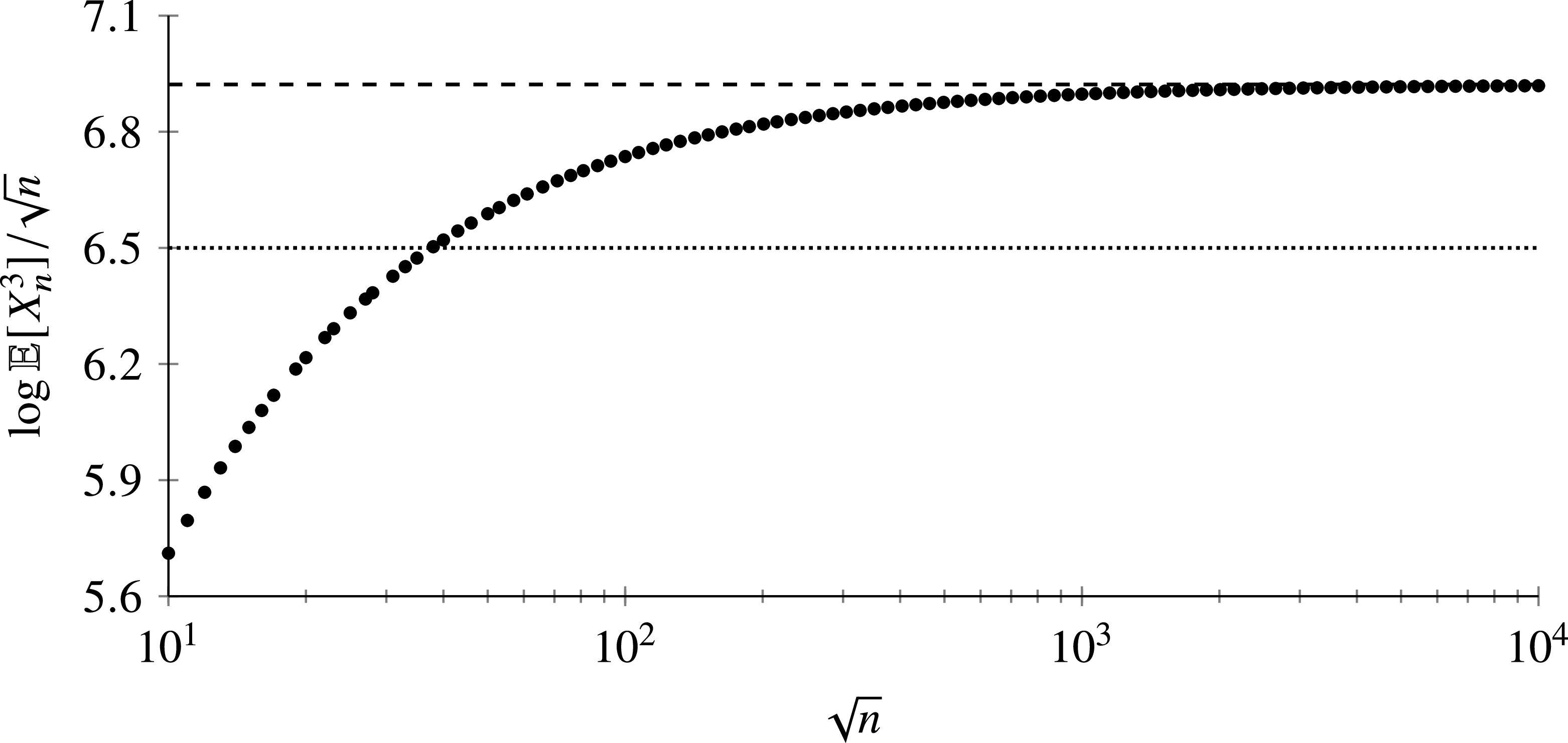
Hence, the first N terms in the power series can be enumerated with the help of a computer. The quantity
 $\log \mathbb{E}[X_n^3]/\sqrt{n}$
is shown in Figure 2. In [Reference Ben-Naim and Krapivsky2],
 $\log \mathbb{E}[X_n^3]/\sqrt{n}$
was computed via simulation to
 $\sqrt{n} \approx 30$
which, due to this sequence’s slow convergence rate, leads to an underestimate of the true value.
The convergence of
 $\log \mathbb{E}[X_n^3]/\sqrt{n}$
to its limiting value. The dashed line is
 $c_3$
from (4.3), and the dotted line is the numerical estimate of [Reference Ben-Naim and Krapivsky2].

5. Proofs of the main steps
5.1. Proof of Lemma 3.1
We take
 $n \to n + 1$
in (3.1), then apply (1.1) raised to the power of q expanded out with the binomial theorem to obtain
 \begin{equation*} C_{n + 1}^{(m)}(q; \, \mathfrak{p}) = \sum_{\beta = 0}^{q}\binom{q}{\beta}\sum_{\alpha_1 = 0}^{n}\sum_{\alpha_2 = 0}^{n}\cdots\sum_{\alpha_{|\mathfrak{p}|} = 0}^{n} \mathbb{E}\Bigg[ X_{n}^\beta X_{U(n)}^{q - \beta} \prod_{\ell = 1}^{| \mathfrak{p} |} X^{p_\ell}_{\alpha_\ell} \Bigg].\end{equation*}
We apply the usual method of conditioning on the value of U(n) inside the expectation. We expand the result into three lines, which will be analyzed sequentially:
 \begin{align} C_{n + 1}^{(m)}(q; \, \mathfrak{p}) & = \sum_{\alpha_1 = 0}^{n}\sum_{\alpha_2 = 0}^{n}\cdots\sum_{\alpha_{| \mathfrak{p} |} = 0}^{n} \mathbb{E}\Bigg[X_{n}^q\prod_{\ell = 1}^{|\mathfrak{p}|}X^{p_\ell}_{\alpha_\ell}\Bigg] \\[-10pt] \nonumber \end{align}
 \begin{align} & \quad + \frac{1}{n + 1}\sum_{\beta = 1}^{q - 1}\binom{q}{\beta} \sum_{\alpha_1 = 0}^{n}\sum_{\alpha_2 = 0}^{n}\cdots\sum_{\alpha_{| \mathfrak{p} |} = 0}^{n}\sum_{\gamma = 0}^{n} \mathbb{E}\Bigg[X_{n}^\beta X_{\gamma}^{q - \beta}\prod_{\ell = 1}^{|\mathfrak{p}|}X^{p_\ell}_{\alpha_\ell}\Bigg] \\[-10pt] \nonumber \end{align}
 \begin{align} & \quad + \frac{1}{n + 1}\sum_{\alpha_1 = 0}^{n}\sum_{\alpha_2 = 0}^{n}\cdots \sum_{\alpha_{| \mathfrak{p} |} = 0}^{n}\sum_{\gamma = 0}^{n} \mathbb{E}\Bigg[X_{\gamma}^{q} \prod_{\ell = 1}^{| \mathfrak{p} |} X^{p_\ell}_{\alpha_\ell} \Bigg]. \\[10pt] \nonumber \end{align}
First, we examine the term in (5.1a). We must write this in terms of sums which extend to
 $n - 1$
rather than n to compare with (3.1). To see how this is done, we note that each sum
 $\sum_{\alpha_i =0}^{n}$
can be expanded to two kinds of terms: one when
 $\alpha_i = n$
and one for
 $\sum_{\alpha_i =0}^{n-1}$
. Therefore, we can write all the sums as a single sum over every possible binary vector of length
 $| \mathfrak{p} |$
such that a 1 in the
 $\ell$
th entry means that
 $\alpha_\ell = n$
and a 0 means
 $\sum_{\alpha_\ell =0}^{n - 1}$
. Consider such a binary vector v whose entries are not all 0 and not all 1, let
 $v_{0, 1}, v_{0, 2}, \dots, v_{0, N_0}$
be the elements of
 $\{\ell \colon v_\ell = 0\}$
, and let
 $v_{1, 1}, v_{1, 2}, \dots, v_{1, N_1}$
be the elements of
 $\{\ell \colon v_\ell = 1\}$
. The contribution to the total sum from v is
 \begin{equation*} \mathbb{E}\Bigg[X_{n}^q\prod_{p_\ell \in \mathfrak{p}}X^{p_\ell}_{\alpha_\ell}\Bigg]_{v} = \sum_{\alpha_{v_{0, 1}} = 0}^{n-1}\sum_{\alpha_{v_{0, 2}} = 0}^{n-1}\cdots\sum_{\alpha_{v_{0, N_0}} = 0}^{n-1} \mathbb{E}\Bigg[ X_{n}^{q + \sum_{i = 1}^{N_1} p_{v_{1, i}} } \prod_{\ell = 1}^{N_0} X^{p_{v_{0, \ell}}}_{\alpha_{v_{0, \ell}}} \Bigg].\end{equation*}
The cases where v consists of all 1s or all 0s lead to the same formula with the appropriate sums omitted.
The sum over all binary vectors v can be equivalently expressed as a sum over every possible multisubset of
 $\mathfrak{p}$
so that the term in (5.1a) can be written as
 \begin{equation} \sum_{\mathfrak{b} \subseteq \mathfrak{p}} C_{n}^{(m)} (q + \lVert \mathfrak{b} \rVert ; \, \mathfrak{p} - \mathfrak{b}).\end{equation}
The term in (5.1b) is similar except for the sum over
 $\gamma$
. By treating
 $q - \beta$
as a part, we can write it as
 \begin{equation} \sum_{\beta = 1}^{q - 1}\binom{q}{\beta}\sum_{\mathfrak{b} \subseteq \mathfrak{p} + [q - \beta ]} \hat{C}_{n}^{(m)}(\beta + \lVert \mathfrak{b} \rVert ; \, \mathfrak{p} + [q - \beta] - \mathfrak{b}),\end{equation}
with reference to the notation of (3.2). The term in (5.1c) requires more attention. Temporarily ignoring the factor of
 $1/(n+1)$
, we will write
 \begin{align} D_{n}^{(m)}(q; \, \mathfrak{p}) & = \sum_{\alpha_1 = 0}^{n}\sum_{\alpha_2 = 0}^{n}\cdots\sum_{\alpha_{| \mathfrak{p} |} = 0}^{n}\sum_{\gamma = 0}^{n} \mathbb{E}\Bigg[X_{\gamma}^{q} \prod_{\ell = 1}^{| \mathfrak{p} |} X^{p_\ell}_{\alpha_\ell} \Bigg] \nonumber \\[3pt] & = \sum_{\substack{\mathfrak{b} \subseteq \mathfrak{p} + [q ] \\[3pt] \mathfrak{b} \neq \varnothing}} C_{n}^{(m)}(\lVert \mathfrak{b} \rVert ; \, \mathfrak{p} + [q] - \mathfrak{b}) + D_{n - 1}^{(m)}(q; \, \mathfrak{p}). \end{align}
In (5.4), the
 $\mathfrak{b} = \varnothing$
term has been separated; note that
 $\mathfrak{b} = \varnothing$
corresponds to the case where no
 $\alpha_i$
is equal to n and hence there is no term of the form
 $X_n^\ell$
inside the expectation so no identification with (3.1) is possible. But then, (5.4) is a linear recurrence relation for
 $D_{n}^{(m)}$
which can be directly solved to obtain
 \begin{equation} D_{n}^{(m)}(q; \, \mathfrak{p}) = \sum_{\ell = 0}^{n}\sum_{\substack{\mathfrak{b} \subseteq \mathfrak{p} + [q ] \\[3pt] \mathfrak{b} \neq \varnothing}} C_{\ell}^{(m)}(\lVert \mathfrak{b} \rVert ; \, \mathfrak{p} + [q] - \mathfrak{b}),\end{equation}
and so, by again referencing the notation of (3.2), the term in (5.1c) can be written as
 \begin{equation} \sum_{\substack{\mathfrak{b} \subseteq \mathfrak{p} + [q ] \\[3pt] \mathfrak{b} \neq \varnothing}} \overline{C}_{n}^{(m)}(\lVert \mathfrak{b} \rVert ; \, \mathfrak{p} + [q] - \mathfrak{b}).\end{equation}
5.2. Proof of Lemma 3.2
First, consider
 $(q; \, \mathfrak{p})_i$
and
 $(q; \, \mathfrak{p})_j$
where
 $i > j$
for a given m. We will say that there is a path of length 1 from
 $(q; \, \mathfrak{p})_i$
to
 $(q; \, \mathfrak{p})_j$
if there exists a
 $\mathfrak{b} \subseteq \mathfrak{p}_i$
such that
 $(q_i + \lVert \mathfrak{b} \rVert; \, \mathfrak{p}_i -\mathfrak{b}) = (q; \, \mathfrak{p})_j$
. Recalling that
 $(q; \, \mathfrak{p})_\ell$
is constrained by
 $q_\ell + \lVert \mathfrak{p} \rVert_\ell = m$
for all
 $\ell$
, if
 $\mathfrak{p}_i - \mathfrak{b} = \mathfrak{p}_j$
, then
 $\lVert \mathfrak{b} \rVert = \lVert \mathfrak{p}_{\mathfrak{i}} \rVert - \lVert \mathfrak{p}_{\mathfrak{j}} \rVert$
, and hence
 $q_i + \lVert \mathfrak{b} \rVert = (m - \lVert \mathfrak{p}_{\mathfrak{i}} \rVert) + (\lVert \mathfrak{p}_{\mathfrak{i}} \rVert - \lVert \mathfrak{p}_{\mathfrak{j}} \rVert) = q_j$
automatically. Therefore, for a path of length 1 to exist, it is necessary and sufficient that
 $\mathfrak{p}_i \supset \mathfrak{p}_j$
. For example, there are two paths of length 1 from
 $(1; \, [1, 1])$
to
 $(2; \, [1])$
, one for each
 $\mathfrak{b} =[1] \subset [1, 1]$
. A path of length k from
 $(q; \, \mathfrak{p})_i$
to
 $(q; \, \mathfrak{p})_j$
is a sequence of k paths of length 1 in which the endpoint of each is the starting point of the next, beginning at
 $(q; \, \mathfrak{p})_i$
and ending at
 $(q; \, \mathfrak{p})_j$
. Two paths are distinct if they differ in any intermediate
 $(q; \, \mathfrak{p})_\ell$
or in any choice of
 $\mathfrak{b}$
. For example, there are two paths of length 2 from
 $(1; \, [1,1])$
to
 $(3; \, \varnothing)$
. Any such path must pass through
 $(2; \, [1])$
, and each consists of one of the two paths of length 1 from
 $(1; \, [1,1])$
to
 $(2; \, [1])$
, followed by the single path of length 1 from
 $(2; \, [1])$
to
 $(3; \, \varnothing)$
with
 $\mathfrak{b} = [1]$
. Note that these are distinct from the single path of length 1 from
 $(1; \, [1, 1])$
to
 $(3; \, \varnothing)$
obtained by choosing
 $\mathfrak{b} = [1, 1]$
immediately.
To establish Lemma 3.2, we must investigate the properties of
 $\mathbf{C}_1$
,
 $\mathbf{C}_2$
, and
 $\mathbf{C}_3$
. The sizes and entries of these matrices all depend on m, and the arguments in this section apply for any
 $m \geq 1$
. As per (3.11), the matrix
 $(\mathbf{I} - z \mathbf{C}_1)^{-1}$
will be important; we therefore begin by studying the properties of
 $\mathbf{C}_1$
. By Proposition 3.1, we can write
 \begin{equation} \mathbf{C}_1 = \mathbf{I} + \mathbf{C}_1',\end{equation}
where
 $\mathbf{C}_1'$
is lower triangular with zeros on its diagonal. The following proposition provides a full characterization of the entries of
 $\mathbf{C}_1'$
and its powers in terms of paths.
Proposition 5.1. For any
 $m \geq 1$
and for
 $1 \leq j < i \leq \mathfrak{C}(m)$
, let
 $[\mathbf{C}_1']^k_{i, j}$
be the entries of the
 $(k\geq 1)$
th power of the matrix
 $\mathbf{C}_1'$
defined in (5.7). The value of
 $[\mathbf{C}_1']^k_{i, j}$
is equal to the number of paths of length k from
 $(q, \mathfrak{p})_i$
to
 $(q, \mathfrak{p})_j$
. Explicitly,
 \begin{equation} [\mathbf{C}_1']^k_{i, j} = \begin{cases} k!\,S_2(|\mathfrak{p}_{i}| - |\mathfrak{p}_{j}|,k) \displaystyle\prod_{v \geq 1}\displaystyle\binom{\phi(\mathfrak{p}_i, v)}{\phi(\mathfrak{p}_j, v)}, & \mathfrak{p}_j \subset \mathfrak{p}_i,\ 1 \leq k \leq | \mathfrak{p}_{i} | - | \mathfrak{p}_{j} |, \\[3pt] 0, & \text{otherwise}, \end{cases} \end{equation}
where
 $S_2(d, k)$
is the Stirling number of the second kind and
 $\phi(\mathfrak{p}, v)$
is the multiplicity of v in
 $\mathfrak{p}$
.
Proof. The proof is by induction on k. The base case
 $k = 1$
follows immediately from the definition in (3.4a), namely that the sum is over
 $(q + \lVert \mathfrak{b} \rVert; \, \mathfrak{p} - \mathfrak{b})$
for
 $\mathfrak{b} \subseteq \mathfrak{p}$
, i.e. the total number of paths of length 1. For the induction step, consider
 \begin{equation} [\mathbf{C}_1']^{k + 1}_{i, j} = \sum_{r = 1}^{\mathfrak{C}(m)} [\mathbf{C}_1']^{k}_{i, r} [\mathbf{C}_1']_{r, j}. \end{equation}
By the induction hypothesis,
 $[\mathbf{C}_1']^{k}_{i, r}$
is equal to the number of paths of length k from
 $(q, \mathfrak{p})_i$
to
 $(q, \mathfrak{p})_r$
, and by the base case,
 $[\mathbf{C}_1']_{r, j}$
is equal to the number of paths of length 1 from
 $(q, \mathfrak{p})_r$
to
 $(q, \mathfrak{p})_j$
; (5.9) is therefore by definition the total number of paths of length
 $k + 1$
from
 $(q, \mathfrak{p})_i$
to
 $(q, \mathfrak{p})_j$
, conditioned on the second last stop of the path. This completes the induction step and hence the proof that
 $[\mathbf{C}_1']^k_{i, j}$
counts paths.
To obtain (5.8), note that we have the combinatorial problem of counting the number of nested subset sequences of length k from a multiset
 $\mathfrak{p}_i$
to one of its multisubsets
 $\mathfrak{p}_j$
. Since multisubsets are counted with multiplicity, the parts of
 $\mathfrak{p}_i$
may be treated as distinguishable. Any
 $v \in \mathfrak{p}_j$
appears
 $\phi(\mathfrak{p}_i, v)$
times in
 $\mathfrak{p}_i$
, and
 $\mathfrak{p}_j$
is made of any
 $\phi(\mathfrak{p}_j, v)$
of them. Hence, there are
 $\prod_{v \geq 1} \binom{\phi(\mathfrak{p}_i, v)}{\phi(\mathfrak{p}_j, v)}$
ways of choosing a particular
 $\mathfrak{p}_j$
. Then,
 $S_2(| \mathfrak{p}_{i} | - | \mathfrak{p}_{j} |, k)$
counts the number of ways of making k intermediate choices of
 $\mathfrak{b}$
from the
 $| \mathfrak{p}_{i} | - | \mathfrak{p}_{j} |$
remaining elements. Finally, these choices of
 $\mathfrak{b}$
can be made in any of the
 $k!$
possible orderings. Collecting these terms gives the non-zero case of (5.8). If
 $\mathfrak{p}_j \not\subset \mathfrak{p}_i$
, then by definition there is no path of length 1 (and hence, of any length) between them, so
 $[\mathbf{C}_1']^{k}_{i, j} = 0$
in this case. The longest chain of length-1 paths is obtained by choosing a
 $\mathfrak{b}$
such that
 $| \mathfrak{b} | = 1$
, and this can be done exactly
 $| \mathfrak{p}_{i} | - | \mathfrak{p}_{j} |$
times so
 $[\mathbf{C}_1']^{k}_{i, j} = 0$
for greater k. Assembling these gives the zero case of (5.8) and completes the proof.
We briefly illustrate Proposition 5.1 with an example. Consider the following sum, which computes the entries of
 $(\mathbf{C}_1')^2$
:
 \begin{equation} [\mathbf{C}_1']^2_{i, j} = \sum_{k = 1}^{\mathfrak{C}(m)} [\mathbf{C}_1']_{i, k} [\mathbf{C}_1']_{k, j}.\end{equation}
This sum is shown schematically in Figure 3 for a particular term in the
 $m = 4$
case.
In the
 $m = 4$
case, a non-zero term contributing to (5.10) for the calculation of
 $[\mathbf{C}_1']^2_{7, 2}$
. Each arrow is a length-1 path, and their combination forms a length-2 path. These arrows show how the indices i, j are related to
 $(q; \, \mathfrak{p})$
indices in the canonical ordering. Referring to Proposition 5.1, we have
 $[1, 1, 1 ] \supset [1, 1] \supset [1]$
, i.e.
 $\mathfrak{p}_7 \supset \mathfrak{p}_4 \supset \mathfrak{p}_2$
.

Define
 \begin{equation} \mathbf{Q} = \mathbf{I} - z \mathbf{C}_1.\end{equation}
Referring to (5.7), we can write
 $\mathbf{Q} = (1 - z)\mathbf{I} - z \mathbf{C}_1'$
. Therefore, for
 $0 \leq z < 1$
we have
 \begin{equation*} \mathbf{Q}^{-1} = \sum_{k = 0}^{\infty} \frac{z^k}{(1 - z)^{k + 1}} [\mathbf{C}_1']^k,\end{equation*}
where the series terminates, since (5.8) implies that
 $[\mathbf{C}_1']^k = \mathbf{0}$
for
 $k \geq m$
. Upon substitution of (5.8), we have, for
 $\mathfrak{p}_j \subset \mathfrak{p}_i$
,
 \begin{equation*} \mathbf{Q}^{-1}_{i, j} = \prod_{v \geq 1} \binom{\phi(\mathfrak{p}_i, v)}{\phi(\mathfrak{p}_j, v)} \sum_{k = 1}^{| \mathfrak{p}_{i} | - | \mathfrak{p}_{j} |} k! \, S_2(| \mathfrak{p}_{i} | - | \mathfrak{p}_{j} |, k) \frac{z^k}{(1 - z)^{k + 1}},\end{equation*}
while
 $\mathbf{Q}^{-1}_{i, j} = 0$
if
 $\mathfrak{p}_j \not\subset \mathfrak{p}_i$
. Expanding
 $z^k (1 - z)^{-(k + 1)} = \sum_{n \geq k} \binom{n}{k} z^n$
, exchanging the order of summation, and applying the identity
 $\sum_{k} \binom{n}{k} k! \, S_2(x, k) = n^{x}$
gives
 \begin{equation} \mathbf{Q}^{-1}_{i, j} = \prod_{v \geq 1} \binom{\phi(\mathfrak{p}_i, v)}{\phi(\mathfrak{p}_j, v)} \sum_{n = 1}^{\infty} n^{| \mathfrak{p}_{i} | - | \mathfrak{p}_{j} |} z^n = \prod_{v \geq 1} \binom{\phi(\mathfrak{p}_i, v)}{\phi(\mathfrak{p}_j, v)} \frac{z \, A_{| \mathfrak{p}_{i} | - | \mathfrak{p}_{j} |}(z)}{(1 - z)^{| \mathfrak{p}_{i} | - | \mathfrak{p}_{j} | + 1}},\end{equation}
where
 $A_{\ell}(z)$
is the Eulerian polynomial, e.g.
 $A_1(z) = 1$
,
 $A_2(z) = 1 + z$
,
 $A_3(z) = 1 + 4z + z^2$
. Note that
 $A_{\ell}(1) = \ell! \neq 0$
.
We now put
 $u = 1/(1 - z)$
and, referring to (3.12), consider
 $\mathbf{P}^{-1}(u) \mathbf{Q}^{-1}(u) \mathbf{P}(u)$
. The effect of a similarity transformation by
 $\mathbf{P}(u)$
on a matrix with entries
 $(a_{i, j})$
is to transform the entries according to
 $a_{i, j} \to a_{i, j} / u^{| \mathfrak{p}_{i} | - | \mathfrak{p}_{j} |}$
. By (5.12), we have
 \begin{equation} [\mathbf{P}^{-1}(u)\mathbf{Q}^{-1}\mathbf{P}(u)]_{i, j} = u \prod_{v \geq 1} \binom{\phi(\mathfrak{p}_i, v)}{\phi(\mathfrak{p}_j, v)} (1 - u^{-1}) \, A_{| \mathfrak{p}_{i} | - | \mathfrak{p}_{j} |}(1 - u^{-1}).\end{equation}
Define the matrix
 $\mathbf{B}_1$
whose entries are
 \begin{equation} [\mathbf{B}_1]_{i,j} = \begin{cases} \displaystyle (| \mathfrak{p}_{i} | - | \mathfrak{p}_{j} |)! \prod_{v \geq 1} \binom{\phi(\mathfrak{p}_i, v)}{\phi(\mathfrak{p}_j, v)}, & \mathfrak{p}_j \subseteq\mathfrak{p}_i, \\[3pt] 0, & \text{otherwise}. \end{cases}\end{equation}
Then, we can write
 $\mathbf{P}^{-1}(u) \mathbf{Q}^{-1}(u) \mathbf{P}(u) = u \mathbf{B}_1 + \mathbf{B}_2(u)$
, where
 $\mathbf{B}_2(u)$
is a matrix whose entries are polynomials in
 $u^{-1}$
. Define
 $\mathbf{D}(u) = \mathbf{P}^{-1}(u) [\mathbf{C}_1 + \mathbf{C}_2 + u \mathbf{C}_3] \mathbf{P}(u)$
; then, referring to (3.11) and (5.11), we can write
 $\mathbf{P}^{-1}(u) \mathbf{R}(u) \mathbf{P}(u) = (u \mathbf{B}_1 + \mathbf{B}_2(u)) \mathbf{D}(u)$
. We will now study the matrix
 $\mathbf{D}(u)$
. From (3.4), and by the same arguments as in the proof of Proposition 3.1, if entry (i, j) in
 $\mathbf{C}_2$
is non-zero, then
 $| \mathfrak{p}_{i} | - | \mathfrak{p}_{j} | \geq -1$
. Similarly, if entry (i, j) in
 $\mathbf{C}_3$
is non-zero, then
 $| \mathfrak{p}_{i} | - | \mathfrak{p}_{j} | \geq 0$
. Hence, we can write
 $\mathbf{D}(u) = u \mathbf{E} + \mathbf{F}(u)$
, where the entries
 $\mathbf{F}(u)$
are polynomials in
 $u^{-1}$
and the entries of
 $\mathbf{E}$
are obtained by restricting the sum in (3.4b) to the term
 $\mathfrak{b} = \varnothing$
and by restricting the sum in (3.4c) to terms where
 $| \mathfrak{b} | = 1$
. Explicitly, in a row indexed by
 $(q; \, \mathfrak{p})$
, the non-zero entries are either indexed by
 $(\beta; \, \mathfrak{p} + [q - \beta])$
for some
 $1 \leq \beta \leq q - 1$
or by
 $(p; \, \mathfrak{p} + [q] - [p])$
where
 $[p] \subseteq \mathfrak{p} + [q]$
. That is,
 \begin{equation} [\mathbf{E}]_{i, j} = \begin{cases} \dbinom{q_i}{q_j}, & \mathfrak{p}_j = \mathfrak{p}_i + [q_i - q_j], \\[3pt] \phi(\mathfrak{p}_i + [q_i], q_j), & [q_j] \subseteq \mathfrak{p}_i + [q_i] \text{ and } \mathfrak{p}_j = \mathfrak{p}_i + [q_i] - [q_j], \\[3pt] 0, & \text{otherwise}. \end{cases}\end{equation}
The two cases cannot contribute to the same entry, since
 $| \mathfrak{p}_{j} | = | \mathfrak{p}_{i} | + 1$
in the first case and
 $| \mathfrak{p}_{j} | =| \mathfrak{p}_{i} |$
in the second.
Next, note that
 \begin{equation*} \mathbf{P}^{-1}(u) \frac{\text{d}}{\text{d} u} \mathbf{P} = u^{-1} \cdot \text{diag}\{| \mathfrak{p}_{1} |, | \mathfrak{p}_{2} |, \dots, | \mathfrak{p}_{\mathfrak{C}(m)} |\} \, =\!: \, u^{-1} \mathbf{J};\end{equation*}
hence, by referring to (3.12), we can now write
 \begin{align*} h'(u) & = -\mathbf{P}^{-1}(u)\mathbf{P}'(u)h(u) + u^{-2}\mathbf{P}^{-1}(u)\mathbf{R}(u)\mathbf{P}(u)h(u) \\[3pt] & = -u^{-1}\mathbf{J}h(u) + u^{-2}(u\mathbf{B}_1 + \mathbf{B}_2)(u\mathbf{E} + \mathbf{F}(u))h(u) \\[3pt] & = \bigg[\mathbf{B}_1\mathbf{E} + \frac{1}{u}(\mathbf{B}_1 \mathbf{F}(u) + \mathbf{B}_2(u)\mathbf{E} - \mathbf{J}) + \frac{1}{u^2}\mathbf{B}_2(u)\mathbf{F}(u)\bigg]h(u),\end{align*}
where
 $\mathbf{F}(u)$
and
 $\mathbf{B}_2(u)$
can each be written as a finite sum of constant matrices multiplied by non-negative powers of
 $u^{-1}$
. Hence, to complete the proof of Lemma 3.2 we need only establish that
 $\mathbf{B}_1 \mathbf{E}$
is a primitive matrix with the appropriate bounds on its Perron–Frobenius eigenvalue, which is the subject of the following proposition. Then, Lemma 3.2 holds with
 $\mathbf{M}_0 = \mathbf{B}_1 \mathbf{E}$
.
Proposition 5.2. The matrix
 $\mathbf{B}_1 \mathbf{E}$
is primitive, where
 $\mathbf{B}_1$
is defined in (5.14) and
 $\mathbf{E}$
is defined in (5.15). The Perron–Frobenius eigenvalue of
 $\mathbf{B}_1 \mathbf{E}$
is bounded above by
 $2^{m+1} (m/{\mathrm{e}})^m {\mathrm{e}}^{6 \sqrt{m}}$
.
Proof. To show that
 $\mathbf{B}_1 \mathbf{E}$
is primitive, since all of its entries are non-negative and since its diagonal entries are all positive, it will be enough to show that the adjacency graph defined by
 $\mathbf{B}_1 \mathbf{E}$
with vertices labelled by the
 $(q, \mathfrak{p})_i$
is strongly connected. From (5.14), we immediately see that
 $[\mathbf{B}_1]_{i,i} = 1$
. From (5.15), taking
 $q_j = q_i$
in the second case shows that the diagonal entries satisfy
 $[\mathbf{E}]_{i, i} = \phi(\mathfrak{p}_i, q_i) + 1 \geq 1$
. Therefore, every
 $\mathbf{B}_1$
-edge and every
 $\mathbf{E}$
-edge is also an edge of
 $\mathbf{B}_1 \mathbf{E}$
. Recall that the entries of
 $\mathbf{E}$
imply that
 $(q; \, \mathfrak{p})$
can reach either
 $(\beta; \, \mathfrak{p} + [q - \beta])$
for some
 $1 \leq \beta \leq q - 1$
or by
 $(p; \, \mathfrak{p} + [q] - [p])$
where
 $[p] \subseteq \mathfrak{p} + [q]$
and the entries of
 $\mathbf{B}_1$
imply that
 $(q; \, \mathfrak{p})$
can reach
 $(q + \lVert \mathfrak{b} \rVert, \mathfrak{p} - \mathfrak{b})$
for any
 $\mathfrak{b} \subseteq \mathfrak{p}$
. To demonstrate that the associated adjacency graph is connected, we will show that there is a bidirectional path between any
 $(q; \, \mathfrak{p})$
and
 $(m, \varnothing)$
. Suppose first that we are starting at some
 $(q; \, \mathfrak{p})$
and want to find a path to
 $(m; \, \varnothing)$
. Then,
 $\mathbf{E}$
provides a path from
 $(q; \, \mathfrak{p})$
to itself and
 $\mathbf{B}_1$
provides a path to
 $(m; \, \varnothing)$
. Now we would like to find a path starting from
 $(m; \, \varnothing)$
back to
 $(q; \, \mathfrak{p})$
. First,
 $\mathbf{E}$
provides a path from
 $(m; \, \varnothing)$
to
 $(m - p_1;\, [p_1])$
for each
 $1 \leq p_1 < m$
, then
 $\mathbf{B}_1$
provides a path from
 $(m - p_1;\, [p_1])$
to itself. Iterating this procedure,
 $\mathbf{E}$
provides a path from
 $(m - p_1, [p_1])$
to
 $(m - p_1 - p_2, [p_1 , p_2])$
for each
 $1 \leq p_2 < m - p_1$
, and
 $\mathbf{B}_{\mathbf{1}}$
provides a path from
 $(m - p_1 - p_2, [p_1 , p_2])$
to itself. Further iterating this procedure shows that any
 $(q; \, \mathfrak{p})$
can be reached by choosing
 $p_1, p_2, \dots$
appropriately. This completes the proof that the matrix
 $\mathbf{B}_1 \mathbf{E}$
is primitive.
Now we will establish the appropriate bounds on the Perron–Frobenius eigenvalue
 $\lambda$
of
 $\mathbf{B}_1 \mathbf{E}$
. To do this, we will use the fact that
 $\lambda$
is bounded above by the maximum sum of the rows of
 $\mathbf{B}_1 \mathbf{E}$
. We first examine
 $\mathbf{B}_1$
. Recalling the Vandermonde identity,
 \begin{equation*} \binom{n_1 + \dots + n_p}{m} = \sum_{k_1 + \cdots + k_p = m} \binom{n_1}{k_1} \binom{n_2}{k_2} \cdots \binom{n_p}{k_p}, \end{equation*}
and that
 $\sum_{v \geq 1}\phi(\mathfrak{p}_i, v) = | \mathfrak{p}_{i} |$
, we have
 \begin{equation*} \prod_{v \geq 1} \binom{\phi(\mathfrak{p}_i, v)}{\phi(\mathfrak{p}_j, v)} \leq \sum_{k_1 + k_2 + \cdots = | \mathfrak{p}_{j} |} \prod_{v \geq 1} \binom{\phi(\mathfrak{p}_i, v)}{k_v} = \binom{| \mathfrak{p}_{i} |}{| \mathfrak{p}_{j} |}. \end{equation*}
Therefore, (5.14) provides
 \begin{equation*} [\mathbf{B}_1]_{i, j} \leq (| \mathfrak{p}_{i} | - | \mathfrak{p}_{j} |)! \prod_{v \geq 1} \binom{\phi(\mathfrak{p}_i, v)}{\phi(\mathfrak{p}_j, v)} \leq \frac{| \mathfrak{p}_{i} |!}{| \mathfrak{p}_{j} |!} \leq (m - 1)!, \end{equation*}
where we have used
 $0 \leq | \mathfrak{p}_{\ell} | \leq m - 1$
. Then, (5.15) immediately provides
 $[\mathbf{E}]_{i, j} \leq \binom{m}{\lfloor m/2 \rfloor}$
by using
 $q_\ell \leq m$
for the first case and
 $\phi(\mathfrak{p}_i+[q_i], q_j) \leq | \mathfrak{p}_{i} |+1 \leq m \leq \binom{m}{\lfloor m/2\rfloor}$
for the second. Since no row of these matrices can have more than
 $\mathfrak{C}(m)$
non-zero entries, the largest entry of
 $\mathbf{B}_1 \mathbf{E}$
is bounded above by
 $(m - 1)!\binom{m}{\lfloor m/2 \rfloor} \mathfrak{C}(m)$
. There are
 $\mathfrak{C}(m)$
rows in
 $\mathbf{B}_1 \mathbf{E}$
, so
 $ \lambda \leq (m - 1)! \binom{m}{\lfloor m/2 \rfloor} \mathfrak{C}(m)^2$
.
Finally, we show that
 $\mathfrak{C}(m) \leq {\mathrm{e}}^{3 \sqrt{m}}$
. Since the elements of
 $\mathcal{C}^{(m)}$
are indexed by
 $(q; \, \mathfrak{p})$
with
 $1 \leq q \leq m$
and
 $\mathfrak{p} \in \mathcal{P}(m - q)$
, we have
 $\mathfrak{C}(m) = \sum_{k = 0}^{m - 1} p(k)$
, where
 $p(k) = |\mathcal{P}(k)|$
is the number of partitions of k. Take
 $t = \sqrt{m}$
; then, since
 ${\mathrm{e}}^{(m - k)/t} \geq 1$
for
 $0 \leq k \leq m - 1$
,
 \begin{equation*} \mathfrak{C}(m) \leq {\mathrm{e}}^{m/t}\sum_{k = 0}^{\infty}p(k){\mathrm{e}}^{-k/t} = {\mathrm{e}}^{m/t}\prod_{j = 1}^{\infty}(1 - \mathrm{e}^{-j/t})^{-1}, \end{equation*}
where the equality follows from Euler’s product formula for the generating function of the partition numbers. Expanding the logarithm of the product and summing the resulting geometric series,
 \begin{equation*} \log\prod_{j = 1}^{\infty}(1 - \mathrm{e}^{-j/t})^{-1} = \sum_{r = 1}^{\infty} \frac{1}{r(\mathrm{e}^{r/t} - 1)} \leq t\sum_{r = 1}^{\infty}\frac{1}{r^2} = \frac{\pi^2}{6} t, \end{equation*}
where the inequality uses
 ${\mathrm{e}}^x - 1 \geq x$
. Therefore,
 \begin{equation*} \mathfrak{C}(m) \leq \exp \bigg[\bigg(1 + \frac{\pi^2}{6}\bigg) \sqrt{m}\bigg] \leq {\mathrm{e}}^{3 \sqrt{m}}. \end{equation*}
For
 $m \geq 2$
, we have
 $(m - 1)! \leq 2 (m/{\mathrm{e}})^m$
, which follows from the standard upper Stirling estimate
 $m! \leq {\mathrm{e}} \sqrt{m} \, (m/{\mathrm{e}})^m$
. Combining this with
 $\binom{m}{\lfloor m/2 \rfloor} \leq 2^m$
yields
 $\lambda \leq 2^{m + 1} (m/{\mathrm{e}})^m {\mathrm{e}}^{6 \sqrt{m}}$
. For
 $m = 1$
, the only element of
 $\mathcal{C}^{(1)}$
is
 $(1; \, \varnothing)$
, and (5.14) and (5.15) give
 $\mathbf{B}_1 = \mathbf{E} = (1)$
, so
 $\lambda = 1$
and the bound holds trivially.
Remark 5.1. For a given m,
 $\mathbf{B}_1 \mathbf{E}$
can be easily computed explicitly using (5.14) and (5.15). Then, its Perron–Frobenius eigenvalue
 $\lambda^{(m)}$
can be calculated exactly, in the sense that
 $\lambda^{(m)}$
is characterized as the Perron root of an explicitly computable integer matrix, yielding
 $c_m = 2\sqrt{\lambda^{(m)}}$
in Theorem 1.1.
6. Open problems
Following the computation of the matrix
 $\mathbf{B}_1 \mathbf{E}$
in Section 5.2, the matrix
 $\mathbf{M}_0$
of Lemma 3.2 can be computed exactly for small values of m with the help of a computer. For example, with
 $m = 4$
we have
 \begin{equation*} \mathbf{M}_0(m = 4) = \begin{pmatrix} 1 &\quad 4 &\quad 6 &\quad 0 &\quad 4 &\quad 0 &\quad 0 \\[3pt] 1 &\quad 5 &\quad 6 &\quad 3 &\quad 5 &\quad 3 &\quad 0 \\[3pt] 1 &\quad 4 &\quad 8 &\quad 0 &\quad 4 &\quad 2 &\quad 0 \\[3pt] 2 &\quad 10 &\quad 12 &\quad 7 &\quad 10 &\quad 8 &\quad 2 \\[3pt] 1 &\quad 5 &\quad 6 &\quad 0 &\quad 5 &\quad 0 &\quad 0 \\[3pt] 2 &\quad 9 &\quad 14 &\quad 4 &\quad 9 &\quad 7 &\quad 0 \\[3pt] 6 &\quad 30 &\quad 36 &\quad 21 &\quad 30 &\quad 24 &\quad 10 \\[3pt] \end{pmatrix}.\end{equation*}
By computing the Perron–Frobenius eigenvalues of the
 $\mathbf{M}_0$
for each m, we can calculate the proportionality constants
 $c_m$
in
 $\log \mathbb{E}[X_{n}^{m}] \sim c_m \sqrt{n}$
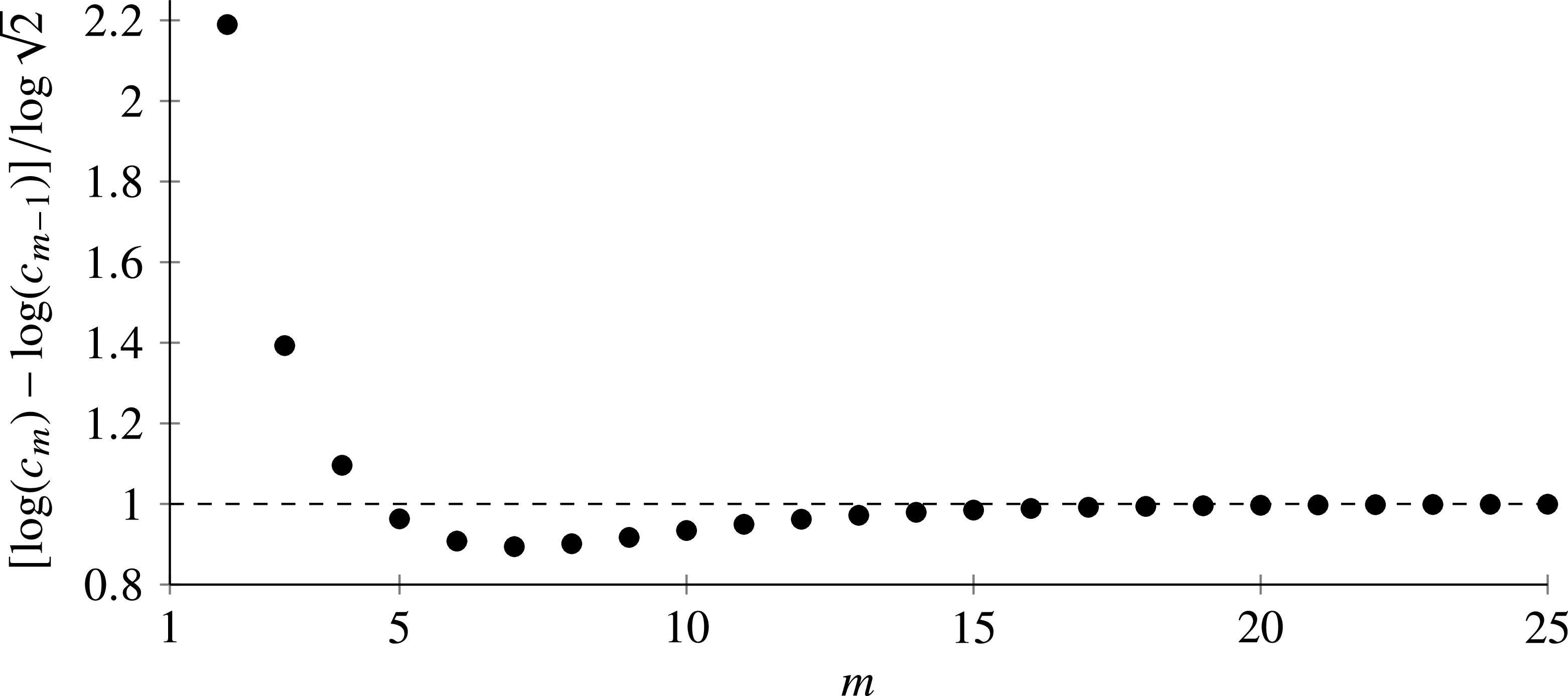
exactly; the quantity
 \begin{equation*} [\!\log\!(c_m) - \log\!(c_{m - 1})]/\log \sqrt{2}\end{equation*}
is shown in Figure 4. Comparing Figure 4 with the bounds provided in Theorem 1.1, it’s clear that the bounds in Theorem 1.1 can be tightened significantly. Based on numerical evidence, we propose the following conjecture.
The values of
 $[\!\log\!(c_m) - \log\!(c_{m - 1})]/\log \sqrt{2}$
provided by computation of the Perron–Frobenius eigenvalue of
 $\mathbf{M}_0$
, where
 $\log \mathbb{E}[X_n^m] \sim c_m \sqrt{n}$
.

Conjecture 6.1. Theorem 1.1 holds with the bounds on
 $c_m$
replaced by the stronger (for large m) bounds
 $\log c_m \in [m \log \sqrt{2},\, m \log \sqrt{2} + 1]$
. Moreover,
 $\log\!(c_m) - \log\!(c_{m - 1}) \to \log \sqrt{2}$
as
 $m \to \infty$
.
Estimating the size of the Perron–Frobenius eigenvalue based on the bounds provided by row and column sums does not appear to be strong enough to obtain this. As observed in [Reference Krasikov, Rodgers and Tripp14], the generalization of the Ulam–Kac adder to (1.4) still admits first and second moments which grow log-asymptotically as
 $\sqrt{n}$
. We therefore propose the following additional conjecture, which can likely be decided with only minor modifications to the arguments in this paper.
Conjecture 6.2. Theorem 1.1 holds for (1.4) with the bounds on
 $c_m$
replaced by
 $[f_1(m, \gamma)$
,
 $f_2(m, \gamma)]$
for suitable functions
 $f_1, f_2$
.
Conjecture 1.2 as well as questions related to the first-passage behavior of the Ulam–Kac adder remain completely open. Many history-dependent random sequences which have been studied recently share the general feature of defining recurrence relations which contain terms of the form
 $X_{U(n)}$
. We considered the case where U(n) is a discrete uniform distribution, but generalizations to non-uniform distributions such as those mentioned in [Reference Krasikov, Rodgers and Tripp14] require further investigation.
Acknowledgements
The author would like to thank Benedek Valkó for providing several very helpful comments on an earlier draft of this paper, as well as Yu-Qiu Zhao for providing a number of references on the asymptotic theory of difference equations. The author would further like to thank the handling editor and anonymous referees for providing a large number of valuable comments, including several simplified arguments and proofs which have been incorporated directly into the text.
Funding information
There are no funding bodies to thank relating to the creation of this article.
Competing interests
There were no competing interests to declare which arose during the preparation or publication process of this article.
Data
The Julia code used to compute the constants
 $c_m$
and to generate the data shown in Figures 2 and 4 is included in the supplementary material.
Supplementary material
The supplementary material for this article can be found at https://doi.org/10.1017/jpr.2026.10136.
 logE[Xn3]/n
 c3

 m=4
 [C1′]7,22
 (q;p)
 [1,1,1]⊃[1,1]⊃[1]
 p7⊃p4⊃p2
 [log(cm)−log(cm−1)]/log2
 M0
 logE[Xnm]∼cmn



