2. Preliminaries

We start with the description of the setting. Let $C[0,\infty)$ denote the space of continuous functions $\omega\,:\, [0,\infty)\mapsto {\mathbb{R}}$ , and let $ \mathcal{C}_t \,:\!= \sigma\{ {\omega}(s)\,:\, s \le t\}$ denote the smallest $\sigma$ -algebra making the coordinate mappings up to time t measurable. Furthermore, let $ \mathcal{C}$ be the smallest $\sigma$ -algebra containing all $\mathcal{C}_t,\, t\geq 0$ . For an interval $I\subset {\mathbb{R}}$ , let ${{(\mathbb{P}_{x}^{X})}_{x\in I}}$ be a family of probability measures defined in the filtered canonical space $\left(C[0,\infty), \mathcal{C}, (\mathcal{C}_t)_{t\geq 0} \right)$ such that, under ${\mathbb{P}}^X_x$ , for a given $x\in I$ the coordinate process $X=(X_t)_{t \ge 0}\,:\!=(\omega_t)_{t \ge 0}$ is a regular diffusion taking values in I and starting from x. Here, X is considered in the sense of Itô and McKean Reference Itô and McKean[8]; see also Reference Borodin and Salminen[2]. A crucial property of X is that there exists a (speed) measure $m^X$ such that the transition probability has a continuous strictly positive density $\left( t,x,y \right)\mapsto {{q}_{t}}\left( x,y \right),t>0,x,y\in I$ with respect to $m^X$ , that is,

(2.1) \begin{equation} {\mathbb{P}}^X_x(X_t\in {\mathrm{d}} y)= q_t(x,y) m^X({\mathrm{d}} y) \label{eqn4} \end{equation}

(see [8, pp. 149 and 157]).

For ${{\left( {{X}_{t}} \right)}_{t\ge 0}},{{X}_{0}}=x$ , as defined above, and $T>0$ , we can construct a new non-homogeneous strong Markov process by conditioning X to be at a given point $y\in I$ at time T. Although the conditioning is generally with respect to a zero set $\{X_T=y\}$ , it can be realized using the Bayes formula and the notion of regular conditional distributions. Another approach is to apply the theory of Doob h-transforms. To explain this briefly, consider X in space–time, i.e. the process $\skew2\bar X=((X_t,t))_{t\geq 0}$ . For $z\in I$ and $t<T$ , introduce the function

\[ h(z,t)\,:\!=h(z,t;\,y,T)\,:\!= q_{T-t}(z,y). \]

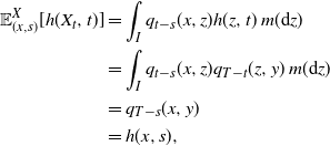
By the Chapman–Kolmogorov equation, for $x\in I$ and $s<t$ we have

\begin{align*} {\mathbb{E}}^X_{(x,s)}[h(X_t,t)]&= \int_I q_{t-s}(x,z)h(z,t)\,m({\mathrm{d}} z)\\ &= \int_Iq_{t-s}(x,z)q_{T-t}(z,y)\,m({\mathrm{d}} z)\\ &= q_{T-s}(x,y)\\ &= h(x,s), \end{align*}

where ${\mathbb{E}}^X_{(x,s)}$ refers to the expectation associated with the space–time process $\skew2\bar X$ initiated from x at time s. Consequently, for $f\in{\cal B}_b(I)$ ( $=$ bounded measurable functions on I) and $s<t<T$ , we may define a non-homogeneous Markov semigroup $ P^{X,h}_{s,t}$ , $0<s<t<T$ , via

(2.2) \begin{equation} P^{X,h}_{s,t}f(x)\,:\!={\mathbb{E}}^X_x\bigg[\:f(X_{t-s})\dfrac{h(X_{t-s},t)}{h(x,s)}\bigg]. \label{eqn5} \end{equation}

The process governed by the probability measure induced by this semigroup is called the X-bridge to y of length T. The notations $X^{x,T,y},\ {\mathbb{P}}^X_{x,T,y}$ , and ${\mathbb{E}}^X_{x,T,y}$ are used for this process, its probability measure, and the expectation, respectively, when the initial state is $x\in I$ . From (2.2) one may deduce the following absolute continuity relation for $A_t\in \mathcal{C}_t,\ t<T$ :

(2.3) \begin{equation} {\mathbb{P}}^X_{x,T,y} (A_t) ={\mathbb{E}}^X_x\bigg[\dfrac{h(X_{t},t)}{h(x,0)}\,;\, A_t\bigg] ={\mathbb{E}}^X_x\bigg[\dfrac{q_{T-t}(X_{t},y)}{q_{T}(x,y)}\,;\, A_t\bigg]. \label{eqn6} \end{equation}

We refer to Chung and Walsh Reference Chung and Walsh[4] for a general discussion of h-transforms, Fitzsimmons, Pitman, and Yor Reference Fitzsimmons, Pitman and Yor[6] (in particular Proposition 1) for general Markovian bridges, and Salminen Reference Salminen[14] for some properties of diffusion bridges.

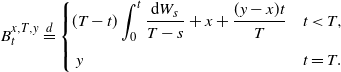
Brownian bridges enjoy several equivalent characterizations in addition to the general h-transform approach. Indeed, a Brownian bridge can be viewed as (i) a Gaussian process, (ii) a deterministic time change with an additional drift of standard Brownian motion, or (iii) as the solution of an SDE; see e.g. [2, p. 66]. In Section 4 we apply (ii) and (iii) in particular. Indeed, (ii) states that

(2.4) $$B_{t}^{x,T,y}\overset{d}{\mathop{=}}\,\left\{ \begin{array}{*{35}{l}} \left( 1-\frac{t}{T} \right){{W}_{{Tt}/{\left( T-t \right)}\;}}+x+\frac{(y-x)t}{T} & t<T, \\ y & t=T, \\ \end{array} \right.$$

where $\stackrel{d}{=} $ means that the processes on the left- and right-hand sides are identical in law, while (iii) says that

(2.5) \begin{align} B^{x,T,y}_t \stackrel{d}{=} \begin{cases} \displaystyle (T-t)\int_0^t \dfrac{{\mathrm{d}} W_s}{T-s} + x +\dfrac{(y-x)t}{T} & t < T , \\[9pt] \ y & t = T. \end{cases} \label{eqn8} \end{align}

Here it is assumed that the canonical filtration ${{({{\mathcal{C}}_{t}})}_{t\ge 0}}$ is augmented with the null sets of $ \mathcal{C}$ with respect to ${\mathbb{P}}_0$ , in order to have the usual conditions satisfied.

3. Main results

3.1. Integral representations for the mean of the first exit time

Let $X=(X_t)_{t\geq 0}$ be a regular diffusion taking values on an interval I, and recall from (2.1) the notation $q_t(x,y)$ for its transition density with respect to the speed measure $m^X$ . For $a<b,\, a,b\in I$ , let $\widehat X$ denote X killed at ${\mathcal{T}}_{(a,b)}$ . Then $\widehat X$ is a regular diffusion on (a,b). 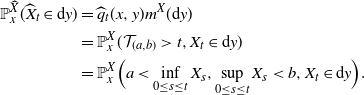The speed measure of $\widehat X$ is $m^X$ , and $\widehat X$ has a continuous strictly positive transition density $\widehat q_t(x,y)$ such that, for $x,y\in(a,b)$ ,

(3.1) \begin{align} {{\mathbb{P}}}^{\widehat X}_x( \widehat X_t \in {\mathrm{d}} y) &= \widehat q_t(x,y) m^X({\mathrm{d}} y) \notag\\ &= {{\mathbb{P}}}^{X}_x( {\mathcal{T}}_{(a,b)}>t, X_t \in {\mathrm{d}} y) \notag \\ &= {{\mathbb{P}}}^{X}_x \Big(a < \inf_{0 \leq s \leq t} X_s, \sup_{0 \leq s \leq t}X_s < b, X_t \in {\mathrm{d}} y\Big). \label{eqn9}\end{align}

This immediately yields the following result.

Proposition 3.1. If ${\mathbb{P}}^X_{x}({\mathcal{T}}_{(a,b)}<\infty)=1$ , i.e. X does not die inside (a,b), we obtain

(3.2) \begin{align} {\mathbb{E}}^X_{x}[{\mathcal{T}}_{(a,b)}] & = \int_{0}^\infty \,{\mathrm{d}} t \int_{a}^{b} m^X({\mathrm{d}} z)\, \widehat q_t(x,z). \label{eqn10} \end{align}

The next proposition will serve as an important tool for the calculations below.

Proposition 3.2. For $x \in (a,b) \subset I$ and $y \in I \backslash (a,b)$ , we have

(3.3) \begin{align} {\mathbb{E}}^X_{x,T,y}[{\mathcal{T}}_{(a,b)}] & = \int_{0}^T \,{\mathrm{d}} t \int_{a}^{b} m^X({\mathrm{d}} z)\, \widehat q_t(x,z) \dfrac{q_{T-t}(z,y)}{q_T(x,y)}. \label{eqn11} \end{align}

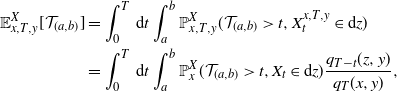
Proof. Since $x\in (a,b)$ and $y \in I \backslash (a,b)$ , we have ${\mathbb{P}}^X_{x,T,y}({\mathcal{T}}_{(a,b)}<T)=1$ . Consider

(3.4) \begin{align} {\mathbb{E}}^X_{x,T,y}[{\mathcal{T}}_{(a,b)}] & = \int_{0}^T \,{\mathrm{d}} t \int_{a}^{b}{\mathbb{P}}^X_{x,T,y}({\mathcal{T}}_{(a,b)}>t,X^{x,T,y}_t\in {\mathrm{d}} z) \notag\\ &= \int_{0}^T \,{\mathrm{d}} t \int_{a}^{b} {{\mathbb{P}}}^X_{x}({\mathcal{T}}_{(a,b)} > t,X_t\in {\mathrm{d}} z) \dfrac{q_{T-t}(z,y)}{q_T(x,y)}, \label{eqn12}\end{align}

where the Markov property and formula (2.2) are used. To get the claimed formula (3.3), it remains to apply (3.1).

3.2. The limit behaviour for regular diffusions

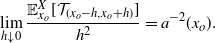
One of our main issues concerns the limiting behaviour of the mean of ${\mathcal{T}}_{ (x-h,x+h )}^X$ as $h\to 0$ for diffusion bridges. For regular diffusions we have the following fairly complete characterization, which has also been proved in Reference Christensen and Lindensjö[3].

Proposition 3.3. Assume that the differential operator associated with the regular diffusion X is given by

\begin{align*} \mathcal{G} u(x)\,:\!= \dfrac{1}{2}a^2(x) u^{\prime\prime}(x) + b(x) u^{\prime}(x), \qquad x \in I, \end{align*}

where $x \mapsto a^2(x) > 0$ and $x \mapsto b(x)$ are continuous in I. Let $x_o \in \mathrm{Int}(I)$ . Then

\begin{align*} \lim_{h \downarrow 0} \dfrac{{\mathbb{E}}_{x_o}^{X}[\mathcal{T}_{(x_o-h,x_o+h)}]}{h^2} = a^{-2}(x_o). \end{align*}

Proof. Recall from [2, part I, chapter II, no. 7, p. 17] that the speed measure $m^X$ and the scale function $s^X$ can be taken to be such that

(3.5) \begin{align} m^{X}({\mathrm{d}} x) = m^X(x) \,{\mathrm{d}} x, \qquad \dfrac{{\mathrm{d}}}{{\mathrm{d}} x}s^X(x) = {\mathrm{e}}^{-B(x)}, \label{eqn13} \end{align}

where

(3.6) \begin{align} m^X(x) = 2a^{-2}(x)\,{\mathrm{e}}^{B(x)}, \qquad B(x) = \int^{x} 2a^{-2}(y) b(y) \,{\mathrm{d}} y. \label{eqn14} \end{align}

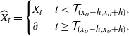
Now consider X initiated at $x_o$ and killed when it leaves the interval $(x_o-h,x_o+h)$ . We let ${{({{\hat{X}}_{t}})}_{t\ge 0}}$ denote this diffusion:

\begin{align*} \widehat{X}_t = \begin{cases} X_t & t < \mathcal{T}_{(x_o-h,x_o+h)},\\ \partial & t \geq \mathcal{T}_{(x_o-h,x_o+h)}, \end{cases} \end{align*}

where $\partial$ is a cemetery point. It is well known (see [2, part I, chapter II, no. 11]) that the 0-resolvent kernel of $\widehat{X}$ is given by

\begin{align*} \widehat{G}_0(x,y) \,:\!= \int_{0}^{\infty} \widehat{q}_t(x,y) \,{\mathrm{d}} t = \begin{cases} \dfrac{(s(x)-s(x_o-h))(s(x_o+h)-s(y))}{s(x_o+h)-s(x_o-h)} & x < y,\\[9pt] \dfrac{(s(y)-s(x_o-h))(s(x_o+h)-s(x))}{s(x_o+h)-s(x_o-h)} & x > y, \end{cases} \end{align*}

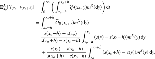
where $s \,:\!= s^X$ and $\widehat{q}_t(x,y)$ is the transition density with respect to the speed measure $m^X$ . Consequently, relation (3.2) implies that

(3.7) \begin{align} {\mathbb{E}}^{X}_{x_o}[\mathcal{T}_{(x_o-h,x_o+h)}] & = \int_0^{\infty} \bigg( \int_{x_o-h}^{x_o+h} \widehat{q}_t(x_o,y) m^X({\mathrm{d}} y) \bigg) \,{\mathrm{d}} t\nonumber\\ & = \int_{x_o-h}^{x_o+h} \widehat{G}_0(x_o,y) m^X({\mathrm{d}} y)\nonumber\\ & = \dfrac{s(x_o{+}h)-s(x_o)}{s(x_o{+}h)-s(x_o{-}h)} \int_{x_o-h}^{x_o} (s(y) - s(x_o{-}h))m^X(y) \,{\mathrm{d}} y\nonumber\\ & \quad\, + \dfrac{s(x_o)-s(x_o{-}h)}{s(x_o{+}h)-s(x_o{-}h)} \int_{x_o}^{x_o+h} (s(x_o{+}h)-s(y)) m^X(y) \,{\mathrm{d}} y. \label{eqn15}\end{align}

Since s is continuously differentiable and $s'(x)>0$ for all x (see (3.5), (3.6)), we have

\begin{align*} \lim_{h \downarrow 0} \dfrac{s(x_o{+}h)-s(x_o)}{s(x_o{+}h)-s(x_o{-}h)} = \lim_{h \downarrow 0} \dfrac{s(x_o)-s(x_o{-}h)}{s(x_o{+}h)-s(x_o{-}h)} = \dfrac{1}{2}, \end{align*}

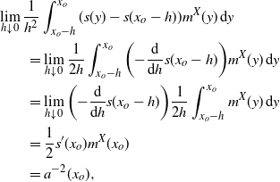
and l’Hôpital’s rule yields

\begin{align*} & \lim_{h \downarrow 0} \dfrac{1}{h^2} \int_{x_o-h}^{x_o} (s(y) - s(x_o-h))m^X(y) \,{\mathrm{d}} y\\ & \qquad = \lim_{h \downarrow 0} \dfrac{1}{2h} \int_{x_o-h}^{x_o} \bigg(\!-\!\dfrac{{\mathrm{d}}}{{\mathrm{d}} h} s(x_o-h) \bigg) m^X(y) \,{\mathrm{d}} y\\ & \qquad = \lim_{h \downarrow 0} \bigg(\!-\!\dfrac{{\mathrm{d}}}{{\mathrm{d}} h} s(x_o-h) \bigg) \dfrac{1}{2h} \int_{x_o-h}^{x_o} m^X(y) \,{\mathrm{d}} y\\ & \qquad = \dfrac{1}{2}s'(x_o)m^X(x_o)\\ & \qquad = a^{-2}(x_o), \end{align*}

where the last equality follows from relations (3.5) and (3.6). Similarly,

\begin{align*} \lim_{h \downarrow 0} \dfrac{1}{h^2} \int_{x_o}^{x_o+h} (s(x_o+h)-s(y))m^X(y) \,{\mathrm{d}} y = a^{-2}(x_o). \end{align*}

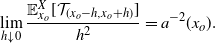
Hence, by (3.7),

\begin{align*} \lim_{h \downarrow 0} \dfrac{{\mathbb{E}}^X_{x_o}[\mathcal{T}_{(x_o-h,x_o+h)}]}{h^2} = a^{-2}(x_o). \end{align*}

3.3. The mean of the first exit time for the Brownian bridge and three-dimensional Bessel bridge

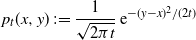
Let

$${{p}_{t}}\left( x,y \right):=\frac{1}{\sqrt{2\pi t}}{{\text{e}}^{{-{{\left( y-x \right)}^{2}}}/{\left( 2t \right)}\;}}$$

denote the transition density of the standard Brownian motion and let

(3.8) \begin{equation} r^{(3)}_t(x,y) \,:\!= \dfrac{y}{x}(p_t(x,y) - p_t(x,-y)), \qquad x,y > 0 \label{eqn16} \end{equation}

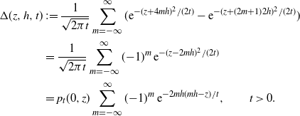
be the transition density of the three-dimensional Bessel process. We also introduce the function

(3.9) $$\begin{array}{*{35}{l}} \Delta \left( z,h,t \right) & :=\frac{1}{\sqrt{2\pi t}}\sum\limits_{m=-\infty }^{\infty }{({{\text{e}}^{-{{{\left( z+4mh \right)}^{2}}}/{\left( 2t \right)}\;}}-{{\text{e}}^{-{{{\left( z+\left( 2m+1 \right)2h \right)}^{2}}}/{\left( 2t \right)}\;}})} \\ {} & =\frac{1}{\sqrt{2\pi t}}\sum\limits_{m=-\infty }^{\infty }{{{(-1)}^{m}}{{\text{e}}^{{-{{\left( z-2mh \right)}^{2}}}/{\left( 2t \right)}\;}}} \\ {} & ={{p}_{t}}\left( 0,z \right)\sum\limits_{m=-\infty }^{\infty }{{{\left( -1 \right)}^{m}}{{\text{e}}^{{-2mh\left( mh-z \right)}/{t}\;}},\qquad t>0.} \\ \end{array}$$

Then, by [2, part II, section 1, 1.15.8 (p. 180)] and (3.9),

(3.10) \begin{align} {\mathbb{P}}_0\Big( \inf_{0 \leq s \leq t} W_s > -h, \sup_{0 \leq s \leq t}W_s < h, W_t \in {\mathrm{d}} z\Big) & = {\mathbb{P}}_0( {\mathcal{T}}_{(\!-\!h,h)} > t, W_t \in {\mathrm{d}} z) \nonumber\\ & =\Delta(z,h,t) \,{\mathrm{d}} z. \label{eqn18}\end{align}

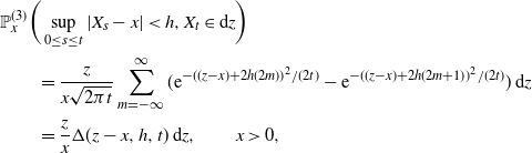
In addition, according to [2, part II, section 5, 1.15.8], for $z \in (x-h,x+h)$ we find that

(3.11) $$\begin{align} & \mathbb{P}_{x}^{\left( 3 \right)}\left( \underset{0\le s\le t}{\mathop{\sup }}\,\left| {{X}_{s}}-x \right|<h,{{X}_{t}}\in \text{d}z \right) \\ & \qquad =\frac{z}{x\sqrt{2\pi t}}\sum\limits_{m=-\infty }^{\infty }{({{\text{e}}^{-{\left( \left( z-x \right)+2h{{\left( 2m \right)}^{2}} \right)}/{\left( 2t \right)}\;}}-{{\text{e}}^{-{{{\left( \left( z-x \right)+2h\left( 2m+1 \right) \right)}^{2}}}/{\left( 2t \right)}\;}})\text{d}z} \\ & \qquad =\frac{z}{x}\Delta \left( z-x,h,t \right)\text{d}z, \qquad x>0, \\ \end{align}$$

where ${\mathbb{P}}^{(3)}$ stands for the probability measure associated with the three-dimensional Bessel process. Finally, let us recall that by [2, part II, section 1, 3.0.6(a)]

(3.12) \begin{align} {\mathbb{P}}_x({\mathcal{T}}_a \in {\mathrm{d}} t,{\mathcal{T}}_a < {\mathcal{T}}_b) = \text{ss}_t(b-x,b-a)\,{\mathrm{d}} t, \qquad a < x < b, \label{eqn20} \end{align}

where the special function $\text{ss}_t$ is given by (see [2, appendix 2, no. 13])

(3.13) $$s{{s}_{t}}\left( a,b \right):=\mathcal{L}_{t,\gamma }^{-1}\left( \frac{\sinh (a\sqrt{2\gamma })}{\sinh (b\sqrt{2\gamma })} \right)=\sum\limits_{m=-\infty }^{\infty }{\frac{b-a+2mb}{\sqrt{2\pi {{t}^{3}}}}{{e}^{{-{{\left( b-a+2mb \right)}^{2}}}/{\left( 2t \right)}\;}}}, \quad a<b,$$

and $\mathcal{L}^{-1}_{t,\gamma}$ denotes the inverse Laplace transform.

Theorem 3.1. (i) bridge-mean For the Brownian bridge with $|y| \geq h$ ,

(3.14) \begin{align} {\mathbb{E}}_{0,T,y}[{\mathcal{T}}_{(\!-\!h,h)}] = \int_{0}^T \int_{-h}^{h} \dfrac{p_{T-t}(z,y)}{p_T(0,y)}\Delta(z,h,t) \,{\mathrm{d}} z \,{\mathrm{d}} t \label{eqn22} \end{align}

and

(3.15) \begin{equation} \lim_{h\downarrow 0} \dfrac{{\mathbb{E}}_{0,T,y}[{\mathcal{T}}_{(\!-\!h,h)}]}{h^2} = 1, \qquad y\neq 0. \label{eqn23} \end{equation}

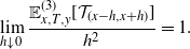
(ii) Bessel-mean For the three-dimensional Bessel bridge with $x>h$ and $y \notin (x-h,x+h)$ ,

\begin{equation*} {\mathbb{E}}^{(3)}_{x,T,y}[{\mathcal{T}}_{(x-h,x+h)}] = \int_{0}^T \int_{-h}^{h} \dfrac{z+x}{x} \Delta(z,h,t)\dfrac{r^{(3)}_{T-t}(z+x,y)}{r^{(3)}_T(x,y)} \,{\mathrm{d}} z \,{\mathrm{d}} t \end{equation*}

and

(3.16) \begin{equation} \lim_{h \downarrow 0} \dfrac{{\mathbb{E}}^{(3)}_{x,T,y}[{\mathcal{T}}_{(x-h,x+h)}]}{h^2} = 1. \label{eqn24} \end{equation}

(iii) If $y \in (\!-\!h,h)$ (or $y \in (x-h,x+h)$ with $x>h$ , $y>0$ ), the mean of the first exit time is infinite for both bridges, that is,

(3.17) \begin{equation} {\mathbb{E}}_{0,T,y}[{\mathcal{T}}_{(\!-\!h,h)}] = {\mathbb{E}}^{(3)}_{x,T,y}[{\mathcal{T}}_{(x-h,x+h)}] = \infty. \label{eqn25} \end{equation}

Proof. (i) According to (3.4), (3.1), and (3.10),

\begin{align*} {\mathbb{E}}_{0,T,y}[{\mathcal{T}}_{(\!-\!h,h)}] = \int_{0}^T \int_{-h}^{h} \dfrac{p_{T-t}(z,y)}{p_T(0,y)}\Delta(z,h,t) \,{\mathrm{d}} z \,{\mathrm{d}} t. \end{align*}

To show (3.15), substitute $z=hu$ and $t=h^2s$ , and note that by the scaling property we have $\Delta(hu,h,h^2 s) h = \Delta(u,1, s)$ , so that

\begin{equation*} {\mathbb{E}}_{0,T,y}[{\mathcal{T}}_{(\!-\!h,h)}] = h^2 \int_{0}^{T/h^2} \int_{-1}^{1} \dfrac{p_{T-h^2s}(hu,y)}{p_T(0,y)}\Delta(u,1, s) \,{\mathrm{d}} u \,{\mathrm{d}} s. \end{equation*}

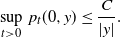
To apply dominated convergence for $h\downarrow 0$ , let y be fixed and assume $h<{\left| y \right|}/{2}\;$ . Then, for any $u \in (\!-\!1,1)$ we have $\left| y-hu \right|>\left| y \right|-h>{\left| y \right|}/{2}\;$ . Moreover, note that for $y\neq0$ there exists a constant $C>0$ such that

(3.18) \begin{equation} \sup_{t>0} \, p_t(0,y)\le \dfrac{C}{|y|}. \label{eqn26} \end{equation}

This implies that

\[ \sup_{u \in (\!-\!1,1), \, s \in (0,T/h^2)} \dfrac{p_{T-h^2s}(hu,y)}{p_T(0,y)} \leq \dfrac{2\, C}{|y|p_T(0,y)}. \]

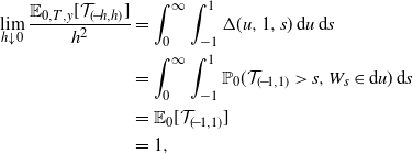
Therefore, as $\left( u,s \right)\mapsto \Delta \left( u,1,s \right)$ is integrable and $\left( u,s,h \right) \mapsto p_{T-h^2s}(hu,y)/p_T\left(0,y \right)$ is bounded on $\left(\!-\!1,1 \right)\times(0,T/h^2) \times \left(0,|y|/2 \right)$ , dominated convergence yields

(3.19) \begin{align} \lim_{h \downarrow 0} \dfrac{{\mathbb{E}}_{0,T,y}[{\mathcal{T}}_{(\!-\!h,h)}]}{h^2} &= \int_{0}^{\infty} \int_{-1}^{1} \Delta(u,1, s) \,{\mathrm{d}} u \,{\mathrm{d}} s \notag\\ &=\int_{0}^{\infty} \int_{-1}^{1} {\mathbb{P}}_0({\mathcal{T}}_{(\!-\!1,1)} >s, W_s \in {\mathrm{d}} u) \,{\mathrm{d}} s \notag \\ &= {\mathbb{E}}_{0} [{\mathcal{T}}_{(\!-\!1,1)}] \notag \\ &= 1, \label{eqn27}\end{align}

where (1.2) is used for the last equality.

(ii) By (3.4), (3.1), and (3.11),

(3.20) \begin{align} {\mathbb{E}}^{(3)}_{x,T,y}[{\mathcal{T}}_{(x{-}h,x{+}h)}] & = \int_{0}^T \int_{x-h}^{x+h} \dfrac{z}{x} \Delta(z-x,h,t) \dfrac{r^{(3)}_{T-t}(z,y)}{r^{(3)}_T(x,y)} \,{\mathrm{d}} z \,{\mathrm{d}} t. \label{eqn28} \end{align}

For the proof of (3.16) we substitute $t=h^2 s$ and $z = hu + x$ and recall that $\Delta (hu, h, h^2 s)h = \Delta(u,1,s)$ , so that

\begin{align*} {\mathbb{E}}^{(3)}_{x,T,y}[{\mathcal{T}}_{(x{-}h,x{+}h)}] & = h^2 \int_{0}^{T/h^2} \int_{-1}^{1} \dfrac{hu+x}{x} \Delta(u,1,s) \dfrac{r^{(3)}_{T-h^2 s}(hu+x,y)}{r^{(3)}_T(x,y)} \,{\mathrm{d}} u \,{\mathrm{d}} s. \end{align*}

Using relation (3.8) yields

\begin{equation*} \bigg| \dfrac{h u + x}{x} \, \dfrac{r^{(3)}_{T-h^2 s}(h u + x,y)}{r^{(3)}_T(x,y)} \bigg| = \bigg| \dfrac{p_{T-h^2 s}(h u + x,y)-p_{T-h^2 s}(h u + x,-y)}{p_T(x,y)-p_T(x,-y)}\bigg|. \end{equation*}

To see that this expression is bounded in $s\in (0, T/h^2)$ and $u \in (\!-\!1,1)$ , note that if $h < |y-x|/2$ with $x>h$ and $y>0$ , then

\[|x-y+hu| > |x-y| - h > |x-y|/2 \quad \text{and} \quad |x+y+hu| > x+y - h > |x-y|/2 ,\]

so that, by (3.18)

\begin{align*} | p_{T-h^2 s}(hu+ x,y)-p_{T-h^2 s}(hu+ x,-y)| \leq \dfrac{C}{|x-y+hu|} + \dfrac{C}{|x+y+hu|} < \dfrac{4C}{|x-y|}. \end{align*}

Hence, dominated convergence gives

\begin{align*} \lim_{h \downarrow 0} \dfrac{{\mathbb{E}}^{(3)}_{x,T,y}[{\mathcal{T}}_{(x{-}h,x{+}h)}]}{h^2} & = \int_{0}^{\infty} \int_{-1}^{1} \Delta(u,1, s) \,{\mathrm{d}} u \,{\mathrm{d}} s =1, \end{align*}

where the last equality was shown in (3.19).

(iii) For a regular diffusion X, (3.17) follows from ${\mathbb{P}}^X_{x,T,y}(\mathcal{T}_{(x-h,x+h)} \ge T)>0$ . To see that this holds, consider

(3.21) \begin{equation} {\mathbb{P}}^X_{x,T,y}({\mathcal{T}}_{(x-h,x+h)} \ge T) = \lim_{\varepsilon \downarrow 0 } \dfrac{ {\mathbb{P}}^X_x({\mathcal{T}}_{(x-h,x+h)} \ge T, y \le X_T \le y+\varepsilon)}{ {\mathbb{P}}^X_x(y \le X_T \le y+\varepsilon)} \label{eqn29} \end{equation}

and

\begin{equation*} {\mathbb{P}}^X_x({\mathcal{T}}_{(x-h,x+h)} \ge T, y \le X_T \le y+\varepsilon) = \int_y^{y+\varepsilon} \widehat q_T(x,z) \,{\mathrm{d}} z, \end{equation*}

where $\widehat q$ is the transition density of X killed at ${\mathcal{T}}_{(x-h,x+h)}$ . By [8, p. 157], the transition density of any regular diffusion is strictly positive. In our case this means

\[\widehat q_T(x,z)> 0 \quad \text{for all } |z|<h. \]

Using l’Hôpital’s rule in (3.21) yields

\begin{equation*} {\mathbb{P}}^X_{x,T,y}({\mathcal{T}}_{(x-h,x+h)} \ge T) = \dfrac{\widehat q_T(x,y)}{q_T(x,y)}>0. \end{equation*}

We also have the following result on convergence in distribution.

Theorem 3.2. For each $y \neq 0$ and $T > 0$ ,

(3.22) \begin{align} \lim_{h \downarrow 0} {\mathbb{E}}_{0,T,y} [{\mathrm{e}}^{-\gamma {\mathcal{T}}_{(\!-\!h,h)}/h^2}] = {\mathbb{E}}_0 [{\mathrm{e}}^{-\gamma {\mathcal{T}}_{(\!-\!1,1)}}], \qquad \gamma > 0{,} \label{eqn30} \end{align}

and, for each $x,y > 0$ ,

\begin{align*} \lim_{h \downarrow 0} {\mathbb{E}}^{(3)}_{x,T,y} [{\mathrm{e}}^{-\gamma {\mathcal{T}}_{(x-h,x+h)}/h^2}] =\lim_{h \downarrow 0} {\mathbb{E}}_{x,T,y} [{\mathrm{e}}^{-\gamma {\mathcal{T}}_{(x-h,x+h)}/h^2}] = {\mathbb{E}}_0 [{\mathrm{e}}^{-\gamma {\mathcal{T}}_{(\!-\!1,1)}}], \qquad \gamma > 0. \end{align*}

Proof. We will sketch the proof of (3.22) since the other result follows similarly. Let

\[{\mathcal{T}}^X_{c} \,:\!= \inf \{ t > 0\colon X_t =c \}\]

denote the first hitting time of c by a continuous process X. Since

\[ {\mathcal{T}}_{(a,b)} = {\mathcal{T}}_{a} \wedge {\mathcal{T}}_{b} = {\mathcal{T}}_{a}{{\bf 1}}_{\{{\mathcal{T}}_{a} < {\mathcal{T}}_b\}} + {\mathcal{T}}_{b}{{\bf 1}}_{\{{\mathcal{T}}_{a} < {\mathcal{T}}_b\}} {,} \]

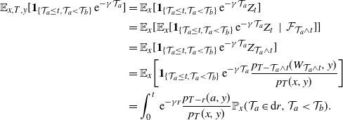
it suffices to consider ${\mathbb{E}}_{x,T,y} [{{\bf 1}}_{\{{{\mathcal{T}}_a < {\mathcal{T}}_b}\}}\,{\mathrm{e}}^{-\gamma {\mathcal{T}}_{a}} ]$ . We recall that by (2.3)

\begin{align*} Z_t(\omega) \,:\!= \dfrac{{\mathrm{d}} {\mathbb{P}}_{x,T,y}}{{\mathrm{d}} {\mathbb{P}}_x} \bigg|_{\mathcal{C}_{t+}}(\omega) = \dfrac{p_{T-t}(\omega(t), y)}{p_T(x,y)},\qquad t < T. \end{align*}

Since $(Z_t)_{t \in [0,T)}$ is a $({\mathbb{P}}_x, (\mathcal{C}_t)_{t \in [0,T)} )$ -martingale and the random variable $ {{\bf 1}}_{\{{ {\mathcal{T}}_a \leq t, {\mathcal{T}}_a < {\mathcal{T}}_b}\}} \,{\mathrm{e}}^{-\gamma {\mathcal{T}}_{a}}$ (with $\gamma>0$ ) is $\mathcal{C}_{{\mathcal{T}}_a \wedge t}$ -measurable, we conclude for $a<x<b$ that

\begin{align*} {\mathbb{E}}_{x,T,y} [{{\bf 1}}_{\{{\mathcal{T}}_a \leq t, {\mathcal{T}}_a < {\mathcal{T}}_b\}}\,{\mathrm{e}}^{-\gamma {\mathcal{T}}_{a}} ] &= {\mathbb{E}}_{x} [{{\bf 1}}_{\{{\mathcal{T}}_a \leq t, {\mathcal{T}}_a < {\mathcal{T}}_b\}} \,{\mathrm{e}}^{-\gamma {\mathcal{T}}_a} Z_t ] \\ &= {\mathbb{E}}_{x} [{{\mathbb{E}}_x [{{\bf 1}}_{\{{\mathcal{T}}_a \leq t, {\mathcal{T}}_a < {\mathcal{T}}_b\}} \,{\mathrm{e}}^{-\gamma {\mathcal{T}}_a} Z_t \mid\mathcal{F}_{{\mathcal{T}}_a \wedge t} ]}] \\ &= {\mathbb{E}}_{x} [{{\bf 1}}_{\{{\mathcal{T}}_a \leq t, {\mathcal{T}}_a < {\mathcal{T}}_b\}} \,{\mathrm{e}}^{-\gamma {\mathcal{T}}_a} Z_{{\mathcal{T}}_a\wedge t} ] \\ &= {\mathbb{E}}_{x}\bigg[{{{\bf 1}}_{\{{\mathcal{T}}_a \leq t, {\mathcal{T}}_a < {\mathcal{T}}_b\}} \,{\mathrm{e}}^{-\gamma {\mathcal{T}}_a}\dfrac{p_{T-{\mathcal{T}}_a\wedge t} ( W_{{\mathcal{T}}_a \wedge t}, y)}{p_T(x,y)}}\bigg] \\ &= \int_{0}^{t} \,{\mathrm{e}}^{-\gamma r} \dfrac{p_{T-r} (a, y)}{p_T(x,y)} {\mathbb{P}}_x({\mathcal{T}}_a \in {\mathrm{d}} r,{\mathcal{T}}_a < {\mathcal{T}}_b ). \end{align*}

Consequently,

\begin{align*} & {\mathbb{E}}_{0,T,y} [{\mathrm{e}}^{-\gamma {\mathcal{T}}_{(\!-\!h,h)}/h^2}]\\ & \quad = \int_{0}^T \,{\mathrm{e}}^{-\gamma r/h^2} \bigg[ \dfrac{p_{T-r} (\!-\!h, y)}{p_T(0,y)} {\mathbb{P}}_0({\mathcal{T}}_{-h} \in {\mathrm{d}} r,{\mathcal{T}}_{-h} < {\mathcal{T}}_h ) + \dfrac{p_{T-r} (h, y)}{p_T(0,y)} {\mathbb{P}}_0({\mathcal{T}}_{h} \in {\mathrm{d}} r,{\mathcal{T}}_{h} < {\mathcal{T}}_{-h})\bigg]. \end{align*}

The result follows by the variable transform $t= r/h^2$ , the scaling property of the Brownian motion and dominated convergence as $h\downarrow 0$ .

Finally we consider the behaviour of the expected hitting time in the case of a three-dimensional Bessel bridge starting at 0.

Theorem 3.3. For the three-dimensional Bessel bridge starting at 0 with $y >h$ ,

(3.23) \begin{align} {\mathbb{E}}^{(3)}_{0,T,y}[{\mathcal{T}}_{h}] & = \int_{0}^T \int_{0}^{h} {\mathbb{P}}^{(3)}_0\bigg(\sup_{0 \leq s \leq t} X_s < h, X_t \in {\mathrm{d}} z\bigg) \dfrac{r^{(3)}_{T-t}(z,y)}{r^{(3)}_T(0,y)}\,{\mathrm{d}} t \label{eqn31} \end{align}

and

\begin{equation*} \lim_{h \downarrow 0} \dfrac{{\mathbb{E}}^{(3)}_{0,T,y}[{\mathcal{T}}_{h}]}{h^2} = \lim_{h \downarrow 0} \dfrac{{\mathbb{E}}^{(3)}_{0}[{\mathcal{T}}_{h}]}{h^2} =\dfrac{1}{3}, \qquad y > 0. \end{equation*}

Proof. The representation (3.23) follows from (3.1) and (3.3), which can be extended to $x=0$ since 0 is an entrance boundary point. Indeed, by [2, part II, section 5, 1.1.8 (p. 435)], for $0< x\vee z<h$ we have

$$\mathbb{P}_{x}^{\left( 3 \right)}\left( \underset{0\le s\le t}{\mathop{\sup }}\,{{X}_{s}}<h,{{X}_{t}}\in \text{d}z \right)=\frac{z}{x\sqrt{2\pi t}}\sum\limits_{m=-\infty }^{\infty }{({{\text{e}}^{{-{{\left( z-x+2mh \right)}^{2}}}/{\left( 2t \right)}\;}}-{{\text{e}}^{{-{{\left( z+x+2mh \right)}^{2}}}/{\left( 2t \right)}\;}})\text{d}z}$$

which implies, as $x \downarrow 0$ ,

\begin{equation*} {\mathbb{P}}^{(3)}_0\bigg(\sup_{0 \leq s \leq t} X_s < h, X_t \in {\mathrm{d}} z\bigg) = 2z \text{ss}_t(h-z,h) \,{\mathrm{d}} z \end{equation*}

with $\text{ss}_t$ as defined in (3.13). Then, relations (3.23) and (3.12) yield

\begin{align*} \lim_{h \downarrow 0} \dfrac{{\mathbb{E}}^{(3)}_{0,T,y}[{\mathcal{T}}_{h}]}{h^2} & = 2 \int_{0}^1 u \int_{0}^{\infty} {\mathbb{P}}_u(\mathcal{T}_0 \in {\mathrm{d}} r, \mathcal{T}_0 < \mathcal{T}_1) \,{\mathrm{d}} u\\ & = 2 \int_{0}^1 u {\mathbb{P}}_u(\mathcal{T}_0 < \mathcal{T}_1) \,{\mathrm{d}} u\\ & = 2 \int_{0}^1 u (1-u) \,{\mathrm{d}} u\\ & = \dfrac{1}{3}. \end{align*}

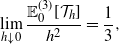
To check that

\[\lim_{h \downarrow 0} \dfrac{{\mathbb{E}}^{(3)}_{0}[{\mathcal{T}}_{h}]}{h^2} =\dfrac{1}{3}{,} \]

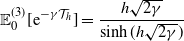
we differentiate the Laplace transform of ${\mathcal{T}}_{h}$ given in [2, part II, section 5, 2.0.1 (p. 469)] as

\[ {\mathbb{E}}^{(3)}_{0}[{\mathrm{e}}^{-\gamma {\mathcal{T}}_{h}}] = \dfrac{h \sqrt{2\gamma}}{\sinh(h\sqrt{2 \gamma}) } \]

with respect to $\gamma$ , and let $\gamma \to 0$ .

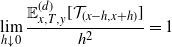
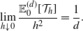
Remark 3.1. We conjecture that for a d-dimensional Bessel bridge starting at $x>0$ , the same limit behaviour

\[ \lim_{h \downarrow 0} \dfrac{{\mathbb{E}}^{(d)}_{x,T,y}[{\mathcal{T}}_{(x-h,x+h)}]}{h^2} = 1 \]

as in Theorem 3.1 holds true. For a d-dimensional Bessel process it can be proved as above in the three-dimensional case that

\[ \lim_{h \downarrow 0} \dfrac{{\mathbb{E}}^{(d)}_{0}[{\mathcal{T}}_{h}]}{h^2} =\dfrac{1}{d}. \]

Hence we conjecture that for a d-dimensional Bessel bridge starting at 0 the limit should also be

\[\lim_{h \downarrow 0} \dfrac{{\mathbb{E}}^{(d)}_{0,T,y}[{\mathcal{T}}_{h}]}{h^2} =\dfrac{1}{d}.\]

3.4. The Kolmogorov distribution function and the mean of the first exit time

A classical result due to Doob Reference Doob[5] is that the distribution of the supremum of the absolute value of the standard Brownian bridge is given by

\begin{equation*} F(h)\,:\!= {\mathbb{P}}_{0,1,0} \bigg(\sup_{0 \leq s \leq 1} |{B_s^{0,1,0}}| \le h \bigg)= \sum_{m=-\infty}^{\infty} (\!-\!1)^m \,{\mathrm{e}}^{-2 m^2 h^2} = \sqrt{2\pi} \Delta(0,h,1), \end{equation*}

where $\Delta$ is as defined in (3.9). The function $h\mapsto F(h),\, h>0$ , is called the Kolmogorov distribution function due to Kolmogorov’s fundamental work Reference Kolmogorov[10] (see also Smirnov Reference Smirnov[16]) on empirical distributions. We refer also to Reference Pitman and Yor[13] and [11, section 5.7]. The main result of this section – Theorem 3.4 – provides representations for the mean of the first exit time of the Brownian bridge and of the three-dimensional Bessel bridge involving the Kolmogorov distribution function.

We now present some formulas related to the Kolmogorov distribution, which we will need later. The following Jacobi theta function identity, an instance of the Poisson summation formula, is stated in [1, equation (2.1)]):

$$\sum\limits_{m=-\infty }^{\infty }{\cos \left( 2m\pi v \right){{\text{e}}^{-{{m}^{2}}{{\pi }^{2}}u}}}=\frac{1}{\sqrt{\pi u}}\sum\limits_{m=-\infty }^{\infty }{{{\text{e}}^{{-{{\left( m+v \right)}^{2}}}/{u}\;}},} \qquad u>0,v\in \mathbb{R}.$$

Setting $u=2x^2/\pi^2$ and $v =1/2$ yields

(3.24) \begin{equation} F(x)=\sum_{m=-\infty}^{\infty} (\!-\!1)^m \,{\mathrm{e}}^{-2 m^2 x^2}= \dfrac{\sqrt{2\pi}}{x} \sum_{k=1}^\infty \exp\bigg(\!-\!\dfrac{(2k-1)^2\pi^2}{8 x^2}\bigg). \label{eqn32} \end{equation}

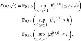
Note also that

\begin{align*} F(h/\sqrt{t}) &= {\mathbb{P}}_{0,1,0} \bigg(\sup_{0 \leq s \leq 1} |{B_s^{0,1 ,0}}| \le h/\sqrt{t} \bigg)\\ &= {\mathbb{P}}_{0,t,0} \bigg( \sup_{0 \leq s \leq 1} |{ B_{ts}^{0,t,0}}| \le h \bigg) \\ &= {\mathbb{P}}_{0,t,0}\bigg( \sup_{0 \leq s \leq t} |{B_s^{0,t ,0}}| \le h\bigg), \end{align*}

where we have used

\[(\sqrt t B_s^{0,1,0})_ {0\leq s\leq 1} \stackrel{d}{=} (B_{st}^{0,t,0})_ {0\leq s\leq 1},\]

which can be seen by applying the scaling property of Brownian motion to the representation (2.4). Consequently,

\begin{equation*} F(h/\sqrt{t}) = {\mathbb{P}}_{0,t,0} ( {\mathcal{T}}_{(\!-\!h,h)}>t )={\mathbb{P}}_{0,t,0} ( {\mathcal{T}}_{(\!-\!h,h)}=\infty ). \end{equation*}

In the following, we will denote the Laplace transform of a function f by

\[\mathcal{L}_{t,\gamma}(\:f(t)) \,:\!= \int_0^\infty \,{\mathrm{e}}^{-\gamma t} f(t) \,{\mathrm{d}} t, \qquad \gamma >0.\]

Note that in this notation the integration variable t is also indicated.

Lemma 3.1. For $|y| \geq h$ ,

(3.25) \begin{align} \int_{0}^T \int_{-h}^{h} p_{T-t}(x,y) \Delta (x,h,t) \,{\mathrm{d}} x \,{\mathrm{d}} t = h \int_{0}^T p_{T-t}(0,y) \Delta (0,h,t)\,{\mathrm{d}} t. \label{eqn33} \end{align}

Proof. We prove Lemma 3.1 by showing that the Laplace transforms of the two sides of (3.25) coincide. Using Fubini’s theorem and the convolution formula, the Laplace transform of the left-hand side of (3.25) is

(3.26) \begin{align} {\mathcal{L}}_{T,\gamma}\bigg(\int_{0}^T \int_{-h}^h p_{T-t}(x,y) \Delta(x,h,t) \,{\mathrm{d}} x \,{\mathrm{d}} t\bigg) = \int_{-h}^h {\mathcal{L}}_{t,\gamma}( p_{t}(x,y) ) {\mathcal{L}}_{t,\gamma} (\Delta(x,h,t)) \,{\mathrm{d}} x. \label{eqn34} \end{align}

To compute the second Laplace transform expression of the right-hand side of (3.26), we use the series representation (3.9). For $x\in (\!-\!h,h)$ ,

$$\left| \sum\limits_{\left| m \right|\ge 2}{{{\left( -1 \right)}^{m}}{{\text{e}}^{{-2mh\left( mh-x \right)}/{t}\;}}} \right|\le {{\sum\limits_{\left| m \right|\ge 2}{\text{e}}}^{{-2mh\left( mh-x \right)}/{t}\;}}\le 2\sum\limits_{m\ge 2}{{{\left( {{\text{e}}^{{-2{{h}^{2}}}/{t}\;}} \right)}^{m}}}\le \frac{2}{1-{{e}^{{-2{{h}^{2}}}/{t}\;}}}.$$

Hence we may interchange the summation and the Laplace transform, and since

\[{\mathcal{L}}_{t,\gamma}(p_{t}(x,z) ) =\dfrac{1}{\sqrt{2 \gamma}} \,{\mathrm{e}}^{- \sqrt{2 \gamma}|z-x|}, \]

we obtain

\begin{align*} \mathcal{L}_{t,\gamma}( \Delta(x,h,t) ) & = {\mathcal{L}}_{t,\gamma} \bigg(\sum_{m=-\infty}^\infty (\!-\!1)^m \,{\mathrm{e}}^{- {2mh(mh-x)}/{t}} \dfrac{ {\mathrm{e}}^{- {x^2}/{2t}}}{\sqrt{2 \pi t}} \bigg) \\ &= \sum_{m=-\infty}^\infty (\!-\!1)^m {\mathcal{L}}_{t,\gamma} ( p_{t}(x,2mh) )\\ &= \dfrac{1}{\sqrt{2\gamma }} \bigg({\mathrm{e}}^{- \sqrt{2 \gamma} |x|} + ({\mathrm{e}}^{ \sqrt{2 \gamma}x} +{\mathrm{e}}^{ -\sqrt{2 \gamma}x})\sum_{m=1}^\infty (\!-\!1)^m \,{\mathrm{e}}^{- \sqrt{2 \gamma}2mh} \bigg)\\ &= {1}/{\bigg[\sqrt{2\gamma} \bigg({\mathrm{e}}^{-\sqrt{2\gamma}|x|} -({\mathrm{e}}^{\sqrt{2\gamma}x} + {\mathrm{e}}^{-\sqrt{2\gamma}x})\dfrac{{\mathrm{e}}^{-\sqrt{2\gamma} 2h}}{1+{\mathrm{e}}^{-\sqrt{2\gamma} 2h}} \bigg)\bigg]}. \end{align*}

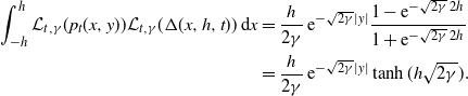
By a straightforward calculation, for the right-hand side of (3.26) we have

(3.27) \begin{align} \int_{-h}^h {\mathcal{L}}_{t,\gamma}(p_{t}(x,y) ){\mathcal{L}}_{t,\gamma}( \Delta(x,h,t) ) \,{\mathrm{d}} x & = \dfrac{h}{2 \gamma} \,{\mathrm{e}}^{- \sqrt{2 \gamma}|y|} \dfrac{1- {\mathrm{e}}^{-\sqrt{2 \gamma} \,2h}}{ 1+ {\mathrm{e}}^{-\sqrt{2 \gamma} \,2h}} \nonumber\\ & = \dfrac{h}{2 \gamma} \,{\mathrm{e}}^{- \sqrt{2 \gamma}|y|} \tanh( h\sqrt{2 \gamma}). \label{eqn35}\end{align}

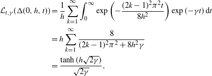
We continue by calculating the Laplace transform of the right-hand side of (3.25). From (3.24),

(3.28) \begin{align} {\mathcal{L}}_{t,\gamma}( \Delta(0,h,t))&= \dfrac{1}{h} \sum_{k=1}^\infty \int_0^\infty \exp\bigg(\!-\!\dfrac{(2k-1)^2\pi^2 t}{8 h^2}\bigg) \exp(\!-\!\gamma t)\,{\mathrm{d}} t \notag \\ &= h \sum_{k=1}^\infty\dfrac{8}{(2k-1)^2\pi^2 + 8 h^2\gamma} \notag\\ &= \dfrac{ \tanh(h\sqrt{2 \gamma})}{\sqrt{2\gamma}}, \label{eqn36}\end{align}

where we have used

\[\tanh\bigg(\dfrac{\pi x}{2} \bigg) = \dfrac{4x}{\pi} \sum_{k=1}^\infty\dfrac{1}{(2k-1)^2 + x^2}, \qquad x \in {\mathbb{R}}\]

(see [7, section 1.421]). By the convolution formula,

(3.29) \begin{align} {\mathcal{L}}_{T,\gamma} \bigg(h \int_{0}^T p_{T-t}(0,y) \Delta(0,h,t) \,{\mathrm{d}} t \bigg) &=h {\mathcal{L}}_{t,\gamma} (p_t(0,y) ){\mathcal{L}}_{t,\gamma} ( \Delta(0,h,t)) \notag \\ &= \dfrac{h}{\sqrt{2 \gamma}} \,{\mathrm{e}}^{- \sqrt{2 \gamma} |y|} \,\, \dfrac{ \tanh( h\sqrt{2 \gamma})}{\sqrt{2 \gamma}}. \label{eqn37}\end{align}

Hence (3.27) and (3.29) coincide, and this finishes the proof of Lemma 3.4.

Theorem 3.4. (i) For the Brownian bridge with $|{y}| \geq h$ ,

(3.30) \begin{align} {\mathbb{E}}_{0,T,y}[{\mathcal{T}}_{(\!-\!h,h)}] &= h \int_0^T \dfrac{ p_{T-t}(0,y)}{p_{T}(0,y)} \Delta(0,h,t) \,{\mathrm{d}} t. \label{eqn38} \end{align}

(ii) For the three-dimensional Bessel bridge with positive $y \notin (x-h,x+h)$ and $x>0$ ,

(3.31) \begin{equation} {\mathbb{E}}^{(3)}_{x,T,y}[{\mathcal{T}}_{(x-h,x+h)}] = h \int_{0}^T \dfrac{r^{(3)}_{T-t}(x,y)}{r^{(3)}_T(x,y)} \Delta(0,h,t) \,{\mathrm{d}} t. \label{eqn39} \end{equation}

Proof. (i) We derive (3.30) from (3.3), (3.1) and Lemma 3.4.

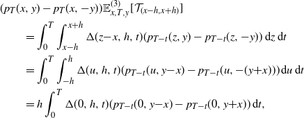
(ii) Recall the relation (3.20). Since, by (3.8),

(3.32) \begin{align} \dfrac{r^{(3)}_{T-t}(z,y)}{r^{(3)}_T(x,y)} = \dfrac{x}{z} \dfrac{p_{T-t}(z,y) - p_{T-t}(z,-y)}{p_T(x,y) - p_T(x,-y)}, \label{eqn40} \end{align}

we have

\begin{align} & (p_T(x,y)-p_T(x,-y)) {\mathbb{E}}^{(3)}_{x,T,y}[{\mathcal{T}}_{(x{-}h,x{+}h)}] \notag\\ & \qquad =\int_{0}^T \int_{x-h}^{x+h} \Delta(z{-}x,h,t) (p_{T-t}(z,y) - p_{T-t}(z,-y)) \,{\mathrm{d}} z \,{\mathrm{d}} t\notag \\ & \qquad = \int_{0}^T\int_{-h}^{h} \Delta(u,h,t)( p_{T-t}(u,y{-}x) - p_{T-t}(u,-(y{+}x))) \,{\mathrm{d}} u \,{\mathrm{d}} t \nonumber\\ & \qquad = h\int_{0}^T \Delta(0,h,t) (p_{T-t}(0,y{-}x) - p_{T-t}(0,y{+}x)) \,{\mathrm{d}} t, \nonumber \end{align}

where the last equality holds by (3.25). Then (3.32) yields (3.31).

Remark 3.2. (i) We have not been able to find a probabilistic explanation for the appearance of the Kolmogorov distribution function in the representations (3.30) and (3.31).

Note that the integrands with respect to t of the expressions in [Theorem 3.1, equation (3.14)] and in [Theorem 3.4, equation (3.30)] do not coincide, that is,

\[ \int_{-h}^h p_{T-t}(z,y) \Delta(z,h,t) \,{\mathrm{d}} z \neq h p_{T-t}(0,y) \Delta(0,h,t).\]

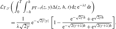
To see this, we can compare the double Laplace transform of

\[ h\, p_{T-t}(0,y) \Delta(0,h,t) \quad \text{and} \quad \int_{-h}^{h} p_{T-t}(z,y) \Delta(z,h,t) \,{\mathrm{d}} z.\]

A computation similar to that in the proof of Lemma 3.1 yields, for $\lambda > 0$ ,

\[ {\mathcal{L}}_{T, \gamma} \bigg( h \int_{0}^T p_{T-t}(0,y) \Delta(0,h,t) \,{\mathrm{e}}^{-\lambda t}\,{\mathrm{d}} t \bigg) = \dfrac{h}{\sqrt{2 \gamma}} \,{\mathrm{e}}^{ - \sqrt{2 \gamma}|y|} \,\, \dfrac{ \tanh( h\sqrt{2 (\gamma+\lambda)})}{\sqrt{2 (\gamma+\lambda)}}. \]

On the other hand, after some calculations,

\begin{align*} & {\mathcal{L}}_{T, \gamma} \bigg(\int_{0}^T \int_{-h}^h p_{T-t}(z,y) \Delta(z,h,t)\,{\mathrm{d}} z \,{\mathrm{e}}^{- \lambda t}\,{\mathrm{d}} t \bigg) \notag \\ & \qquad = \dfrac{1}{ \lambda \sqrt{2 \gamma}} \,{\mathrm{e}}^{- \sqrt{2 \gamma}|y|} \,\, \bigg[ 1- \dfrac{ {\mathrm{e}}^{- \sqrt{2 \gamma}h} + {\mathrm{e}}^{\sqrt{2 \gamma}h} }{ {\mathrm{e}}^{- \sqrt{ 2(\gamma+\lambda)}h} + {\mathrm{e}}^{\sqrt{ 2(\gamma+\lambda)}h} }\bigg]. \end{align*}

(ii) It is also possible to use (3.30) and (3.31) to show (3.15) and (3.16). For example, after the variable transform $t=h^2r$ , we find an integrable majorant and conclude by dominated convergence that

\begin{equation*} h \int_0^T \dfrac{ p_{T-t}(0,y)}{p_{T}(0,y)} \Delta(0,h,t) \,{\mathrm{d}} t \to \int_{0}^{\infty} \Delta(0,1,t) \,{\mathrm{d}} t, \qquad h \downarrow 0. \end{equation*}

Then, by monotone convergence, thanks to relation (3.28) we obtain

\begin{align*} \int_{0}^{\infty} \Delta(0,1,t) \,{\mathrm{d}} t & = \lim_{\gamma \to 0+} \int_{0}^{\infty}\,{\mathrm{e}}^{-\gamma t} \Delta(0,1,t) \,{\mathrm{d}} t = \lim_{\gamma \to 0+} \dfrac{\tanh(\sqrt{2\gamma})}{\sqrt{2 \gamma}} = 1. \end{align*}

We conclude this section by pointing out a connection between the Kolmogorov distribution function and the density of the last visit of 0 by a Brownian motion before ${\mathcal{T}}_{(\!-\!h,h)}$ . This connection was noted by Knight in [9, Corollary 2.1]. Here we provide a different proof of this fact.

Proposition 3.4. When $\widehat W$ is a Brownian motion killed at $\mathcal{T}_{(\!-\!h,h)}$ , then $t\mapsto \left( 1/h \right)\Delta \left( 0,h,t \right)$ is the density of the last passage time $\lambda_0 \,:\!= \sup \{t>0\colon \widehat W_t = 0\}$ .

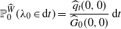
Proof. It is well known that

(3.33) \begin{align} {\mathbb{P}}_0^{\widehat W}(\lambda_0 \in {\mathrm{d}} t) = \dfrac{\widehat q_t(0,0)}{\widehat G_0(0,0)}\,{\mathrm{d}} t \label{eqn41} \end{align}

(see [2, part I, chapter II, no. 20, p. 26]), where

\[\widehat q_t(x,y) = \dfrac{1}{\sqrt{2 \pi t}} \sum_{ m =-\infty}^{\infty} ({{\mathrm{e}}^{-{(x-y+4mh)^2}/{(2t)}} - {\mathrm{e}}^{-{(x+y+(2 m+1)2h)^2}/{(2t)}}}) \]

is the transition density (with respect to the Lebesgue measure) of $\widehat W$ (see [2, part I, appendix I, no. 6, p. 126]), and

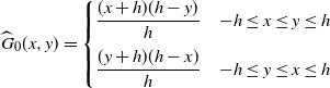\begin{align*} \widehat G_0(x,y) = \begin{cases} {\displaystyle\dfrac{(x+h)(h-y)}{h}} & -h \leq x \leq y \leq h\\[9pt] {\displaystyle \dfrac{(y+h)(h-x)}{h}} & -h \leq y \leq x \leq h \end{cases} \end{align*}

denotes the 0-resolvent kernel (see [2, part I, appendix I, no. 6, p. 126]). Note that $\widehat{q}_t(0,0) = \Delta(0,h,t)$ and $\widehat{G}_0(0,0) = h$ , so from (3.33) we obtain

\begin{align*} {\mathbb{P}}_0^{\widehat W}(\lambda_0 \in {\mathrm{d}} t)/{\mathrm{d}} t = \dfrac{\Delta(0,h,t)}{h}. \end{align*}

4. Application

In this section we apply the previous results and prove in detail an estimate needed in the convergence analysis, presented in Walsh Reference Walsh[17], of a functional of the binomial tree model for a corresponding functional of the Black–Scholes model. This convergence analysis succeeds in identifying the leading constants $C_1,C_2$ appearing in the error expansion

(4.1) \begin{equation} {\mathbb{E}} [g(X^{(n)}_n)- g(X_T)] = C_1 \sqrt{\dfrac{T}{n}} +C_2 \dfrac{T}{n} + {\mathrm{O}}\bigg(\dfrac{1}{n^{3/2}}\bigg), \qquad n \text{ even} \label{eqn42} \end{equation}

(see [17, equation (14)]) in terms of expressions depending on the function g (which is assumed to be exponentially bounded and piecewise twice continuously differentiable). Here $X_t = \sigma W_t$ for $t\ge 0$ and $\left( X_{k}^{\left( n \right)} \right)_{k=0}^{n}$ denotes a symmetric simple random walk with time step $T/n$ and space step size $ \sigma\sqrt{T/n}$ . For simplicity, we will set $\sigma=1$ and hence consider

\[{\mathbb{E}} [g(W^{(n)}_n) - g(W_T)].\]

The central idea of this error analysis is to build the random walk from a given Brownian motion ${{({{W}_{t}})}_{t\ge 0}}$ so that both processes are on the same probability space. Fix $T>0$ and $n \in {\mathbb{N}}$ . For $h\,:\!=\sqrt{T/n}$ , define $\tau_0 \,:\!=0$ and

\begin{equation*} \tau_k \,:\!= \inf\{ t> \tau_{k-1}\colon |W_t-W_{\tau_{k-1}}| = h \}, \qquad k \ge 1. \end{equation*}

Then $\left( {{W}_{{{\tau }_{k}}}}-{{W}_{{{\tau }_{k-1}}}} \right)_{k=1}^{\infty }$ is a sequence of i.i.d. random variables with

\[{\mathbb{P}}( W_{\tau_{k}} -W_{\tau_{k-1}} = h)= {\mathbb{P}}( W_{\tau_{k}} -W_{\tau_{k-1}} = - h)= \dfrac{1}{2}. \]

Let $k_*$ be such that $\tau_{k_*}\le T< \tau_{k_*+1}$ . One central idea to get (4.1) is to split the error into a local part (exploiting the closeness of $W_T$ and $W_{\tau_{k_*+1}}$ ) and a global part (using the binomial distribution), that is,

\[ {\mathbb{E}} [(g(W_T)- g( W_{\tau_{k_*+1}}) ) {{\bf 1}}_{\{ k_* \text{ odd } \}}] + {\mathbb{E}} [ (g( W_{\tau_{k_*+1}})- g( W_{\tau_{n}}) {{\bf 1}}_{\{ k_* \text{ odd } \}}], \]

respectively, while the splitting is done with $W_{\tau_{k_*+2}}$ if $k_* $ is even.

For this, in [17, section 9], where L denotes our $k_* $ , the conditional probability

\begin{equation*} q(x) \,:\!= {\mathbb{P}}( k_* \text{ is even}\mid W_T = x), \qquad x \in {\mathbb{R}} \end{equation*}

is introduced. We want to study and estimate q. The reason for considering only even n and even $k_*+1$ or $k_*+2$ is to avoid even/odd fluctuations known to appear in binomial tree schemes. Note that $ k_*$ is an even number if and only if $W_{\tau_{k_*}}$ is an even multiple of h.

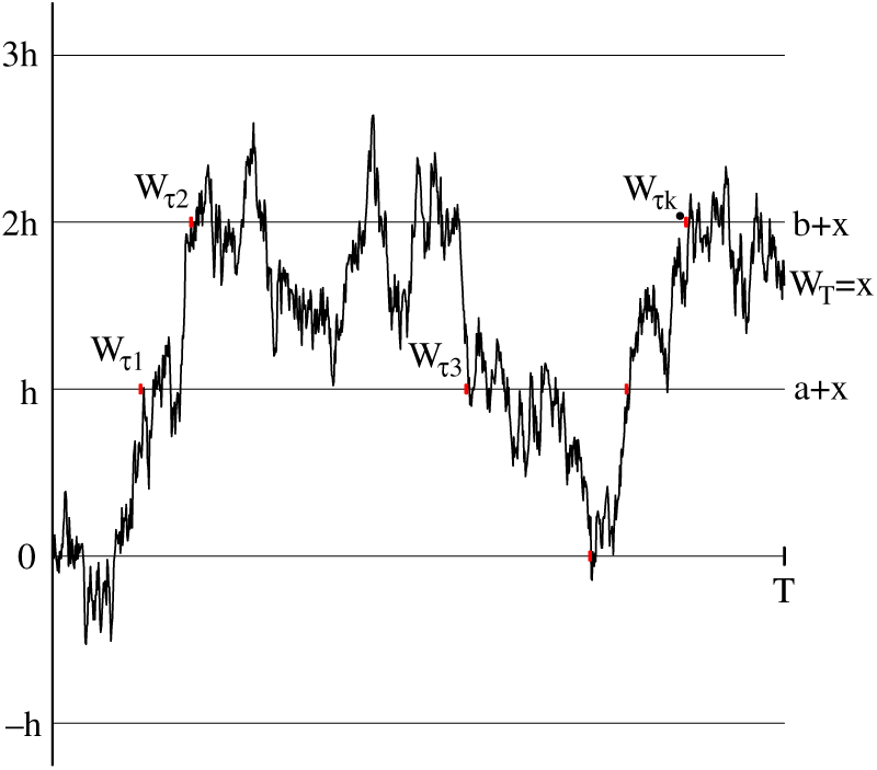
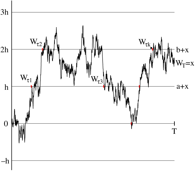
The process ${{\left( {{W}_{t}} \right)}_{0\le t\le T}}$ given $W_0=0, W_T=x$ is identical in law to the bridge ${{\left( B_{t}^{0,T,x} \right)}_{0\le t\le T}}$ . See Figure 1.

Figure 1:

A Brownian motion satisfying $W_0=0, W_T=x$ .

Fix $k \in \mathbb{Z}$ and assume $x \in ((2k-1)h, (2k+1)h)$ . For simplicity, set

(4.2) \begin{equation} \underline{h} \,:\!=(2k-1)h, \qquad \overline{h} \,:\!=(2k+1)h, \qquad h_{e} \,:\!= 2kh \label{eqn43} \end{equation}

for the lower and upper value, and for the ‘even’ midpoint of the interval. Then, given $W_T=x$ , we find that ‘ $k_*$ is even’ is the same as ‘ $W_{\tau_{k_*}}= h_e$ ’. For the time-reversed bridge, i.e. ${{\left( B_{t}^{x,T,0} \right)}_{0\le t\le T}}$ , we get

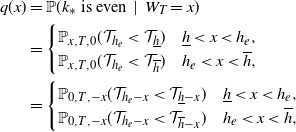\begin{align*} q(x) & = {\mathbb{P}}(k_* \text{ is even}\mid W_T = x)\\ &= \begin{cases} {\mathbb{P}}_{x,T,0}({\mathcal{T}}_{h_e} < {\mathcal{T}}_{\underline{h}}) & \underline{h} <x< h_e,\\ {\mathbb{P}}_{x,T,0}({\mathcal{T}}_{h_e} < {\mathcal{T}}_{\overline{h}}) & h_e < x < \overline{h}, \end{cases} \\ &= \begin{cases} {\mathbb{P}}_{0,T,-x}({\mathcal{T}}_{h_e-x} < {\mathcal{T}}_{\underline{h} -x}) & \underline{h} <x< h_e,\\ {\mathbb{P}}_{0,T,-x}({\mathcal{T}}_{h_e-x} < {\mathcal{T}}_{\overline{h} -x}) & h_e < x < \overline{h}{,} \end{cases} \end{align*}

where ${\mathcal{T}}_y({\omega}) \,:\!= \inf\{t>0\colon \omega(t)=y \}$ for $\omega \in C[0,T]$ . Note that, for any $a < 0 < b$ and $y \notin (a,b)$ ,

\begin{equation*} {\mathbb{E}}_{0,T,y} [B_{{\mathcal{T}}_{(a,b)}}] = a (1-{\mathbb{P}}_{0,T,y}({\mathcal{T}}_b < {\mathcal{T}}_a)) + b \, {\mathbb{P}}_{0,T,y}({\mathcal{T}}_b < {\mathcal{T}}_a), \end{equation*}

and, consequently,

\begin{equation*} {\mathbb{P}}_{0,T,y}({\mathcal{T}}_b < {\mathcal{T}}_a) = \dfrac{-a}{b-a} + \dfrac{ {\mathbb{E}}_{0,T,y} [B_{{\mathcal{T}}_{(a,b)}}]}{b-a}. \end{equation*}

Hence

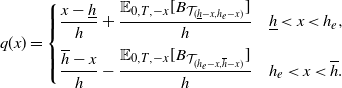(4.3) \begin{align} q(x) = \begin{cases} \dfrac{x-\underline{h} }{h} + \dfrac{ {\mathbb{E}}_{0,T,-x} [B_{{\mathcal{T}}_{( \underline{h} -x, h_e-x )}}]}{h} & \underline{h} <x< h_e, \\[9pt] \dfrac{\overline{h} -x}{h} - \dfrac{ {\mathbb{E}}_{0,T,-x} [B_{{\mathcal{T}}_{(h_e-x, \overline{h}-x )}}]}{h} & h_e < x < \overline{h}. \end{cases} \label{eqn44} \end{align}

Arguing that a Brownian bridge and Brownian motion have similar exit behaviour for small h, Walsh [17, equation (20)] stated that

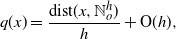(4.4) \begin{equation} q(x) = \dfrac{{\textrm{dist}}(x,{\mathbb{N}}^h_o)}{h} + {\mathrm{O}}(h) , \label{eqn45} \end{equation}

where $x\in {\mathbb{R}}$ , ${\mathbb{N}}^h_o = {\{(2k{+}1)h\colon k \in \mathbb{Z}\}}$ and ${\textrm{dist}}(x,{\mathbb{N}}^h_o) \,:\!= \inf\{|x-y|\colon y\in {\mathbb{N}}^h_o \}$ . Clearly,

\[{\textrm{dist}}(x,{\mathbb{N}}^h_o) \text{ is equal to } x-\underline{h} \,\text{ or }\, \overline{h} -x\ \text{for some } k,\]

so for (4.4) to hold we should have

(4.5) \begin{equation} \bigg|q(x) - \dfrac{{\textrm{dist}}(x,{\mathbb{N}}^h_o)}{h} \bigg| = \bigg| \dfrac{{\mathbb{E}}_{0,T,-x}[B_{{\mathcal{T}}(x)}]}{h} \bigg| = {\mathrm{O}}(h), \label{eqn46} \end{equation}

where (4.2) was used to rewrite ${\mathcal{T}}_{( \underline{h} -x, h_e-x )}$ and ${\mathcal{T}}_{(h_e-x, \overline{h}-x )}$ as

(4.6) \begin{equation} {\mathcal{T}}(x)\,:\!= {\mathcal{T}}_{(kh-x, (k+1)h-x)} \text{ if } x\in (kh, (k+1)h). \label{eqn47} \end{equation}

We will show below that (4.5) is indeed true for a fixed x. However, we will see that this relation does not hold uniformly in x, and therefore it cannot be used to estimate the second term on the right-hand side of (4.11) below. We will estimate that second term in Corollary 4.1 below.

Lemma 4.1. Suppose that $a < 0 < b$ , $y \notin (a,b)$ , $T > 0$ and $h > 0$ . Then

(4.7) \begin{align} | {\mathbb{E}}_{0,T,y} [B_{{\mathcal{T}}_{(a,b)}}] | \le \dfrac{{\mathbb{E}}_{0,T,y}[ {\mathcal{T}}_{(a ,b)}]}{T} (2(|a| \vee b) + |y| + 3\sqrt{2 T}). \label{eqn48} \end{align}

Proof. We use the Markov inequality to deduce

\[ | {\mathbb{E}}_{0,T,y} [ B_{ {\mathcal{T}}_{(a ,b)}} {{\bf 1}}_{\{{\mathcal{T}}_{(a ,b)} > T/2\}} ] | \le (|a| \vee b) {\mathbb{P}}_{0,T,y} ({\mathcal{T}}_{(a ,b)} > T/2) \le \dfrac{2(|a| \vee b)}{T} {\mathbb{E}}_{0,T,y}[ {\mathcal{T}}_{(a ,b)}]. \]

To estimate $ | {\mathbb{E}}_{0,T,y} [ B_{ {\mathcal{T}}_{(a ,b)}} {{\bf 1}}_{\{{\mathcal{T}}_{(a ,b)} \le T/2\}} ] |$ , we use the representation (2.5) for a Brownian bridge:

\[\tilde{B}^{0,T,y}_t\,:\!= (T-t)\int_0^t \dfrac{{\mathrm{d}} W_s}{T-s} + \dfrac{t}{T}y, \quad t \in [0,T), \quad \text{and} \quad \tilde{B}^{0,T,y}_T \,:\!=y.\]

Introducing

\[\tilde{{\mathcal{T}}}\,:\!= \inf\{t\in [0,T]\colon \tilde{B}^{0,T,y}_t \notin (a,b) \}{,}\]

we have

\[ {\mathbb{E}} [\tilde{B}^{0,T,y}_{\tilde{{\mathcal{T}}}} {{\bf 1}}_{\{\tilde{{\mathcal{T}}} \le T/2\}}] = {\mathbb{E}}_{0,T,y} [ B_{ {\mathcal{T}}_{(a ,b)}} {{\bf 1}}_{\{ {\mathcal{T}}_{(a ,b)} \le T/2\}}] \]

and

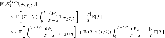\begin{align*} & |{\mathbb{E}} [\tilde{B}^{0,T,y}_{\tilde{{\mathcal{T}}}} {{\bf 1}}_{\{\tilde{{\mathcal{T}}} \le T/2\}}] | \\ &\qquad \le \bigg|{\mathbb{E}} \bigg[(T- \tilde{{\mathcal{T}}}) \int_0^{\tilde{{\mathcal{T}}}} \dfrac{{\mathrm{d}} W_s}{T-s}{{\bf 1}}_{\{\tilde{{\mathcal{T}}} \le T/2\}}\bigg]\bigg| + \dfrac{|y|}{T}{\mathbb{E}} [\tilde{{\mathcal{T}}}] \\ &\qquad \le T \bigg|{\mathbb{E}} \bigg[ \int_0^{\tilde{{\mathcal{T}}} \wedge {T}/{2}} \dfrac{{\mathrm{d}} W_s}{T-s}\,\,{{\bf 1}}_{\{\tilde{{\mathcal{T}}} \le T/2\}}\bigg]\bigg|+ {\mathbb{E}} \bigg|(\tilde{{\mathcal{T}}} \wedge(T/2)) \int_0^{\tilde{{\mathcal{T}}} \wedge {T}/{2}} \dfrac{{\mathrm{d}} W_s}{T-s}\bigg| + \dfrac{|y|}{T}{\mathbb{E}} [\tilde{{\mathcal{T}}}] . \end{align*}

We note that, by the optional stopping theorem,

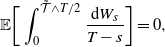\[{\mathbb{E}} \bigg[\int_0^{\tilde{{\mathcal{T}}} \wedge {T}/{2}} \dfrac{{\mathrm{d}} W_s}{T-s}\bigg]=0 {,} \]

so that

\begin{equation*} \bigg|{\mathbb{E}} \bigg[ \int_0^{\tilde{{\mathcal{T}}} \wedge{T}/{2}} \dfrac{{\mathrm{d}} W_s}{T-s} \,\, {{\bf 1}}_{\{\tilde{{\mathcal{T}}} \le T/2\}} \bigg]\bigg| =\bigg|{\mathbb{E}} \bigg[ \int_0^{\tilde{{\mathcal{T}}} \wedge{T}/{2}} \dfrac{{\mathrm{d}} W_s}{T-s} \,\, {{\bf 1}}_{\{\tilde{{\mathcal{T}}} > T/2\}} \bigg]\bigg|. \end{equation*}

Then, by the Cauchy–Schwarz and Markov inequalities,

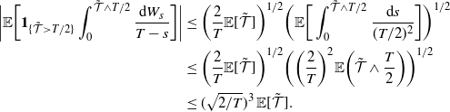\begin{align*} \bigg|{\mathbb{E}} \bigg[ {{\bf 1}}_{\{\tilde{{\mathcal{T}}} > T/2\}} \int_0^{\tilde{{\mathcal{T}}} \wedge{T}/{2}} \dfrac{{\mathrm{d}} W_s}{T-s} \bigg]\bigg| & \le \bigg(\dfrac{2}{T}{\mathbb{E}} [\tilde{{\mathcal{T}}}] \bigg)^{{1}/{2}} \bigg({\mathbb{E}} \bigg[\int_0^{\tilde{{\mathcal{T}}} \wedge{T}/{2}} \dfrac{{\mathrm{d}} s}{(T/2)^2}\bigg] \bigg)^{{1}/{2}} \\ & \le \bigg(\dfrac{2}{T} {\mathbb{E}}[\tilde{{\mathcal{T}}}] \bigg)^{{1}/{2}} \bigg( \bigg(\dfrac{2}{T}\bigg)^2 {\mathbb{E}} \bigg( \tilde{ {\mathcal{T}}} \wedge \dfrac{T}{2} \bigg) \bigg)^{{1}/{2}}\\ & \le (\sqrt{2/T})^3 \, {\mathbb{E}} [\tilde{{\mathcal{T}}}]. \end{align*}

Again by the Cauchy–Schwarz inequality,

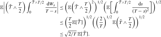\begin{align*} {\mathbb{E}}\bigg| \bigg(\tilde{{\mathcal{T}}} \wedge \dfrac{T}{2} \bigg) \int_0^{\tilde{{\mathcal{T}}} \wedge {T}/{2} } \dfrac{{\mathrm{d}} W_s}{T-s} \bigg| &\le \bigg({\mathbb{E}} \bigg(\tilde{{\mathcal{T}}} \wedge \dfrac{T}{2} \bigg)^2 \bigg)^{{1}/{2}}\bigg({\mathbb{E}} \bigg[\int_0^{\tilde{{\mathcal{T}}} \wedge{T}/{2}} \dfrac{{\mathrm{d}} s}{(T-s)^2}\bigg] \bigg)^{{1}/{2}} \\ & \le \bigg( \dfrac{T}{2} {\mathbb{E}}[\tilde{{\mathcal{T}}}] \bigg)^{{1}/{2}} \bigg( \bigg( \dfrac{2}{T}\bigg)^{{1}/{2}} {\mathbb{E}} \bigg(\tilde{T} \wedge \dfrac{T}{2} \bigg) \bigg)^{{1}/{2}}\\ &\le \sqrt{2/T} \, {\mathbb{E}} [\tilde{{\mathcal{T}}}]. \end{align*}

The above estimates and ${\mathbb{E}}_{0,T,y}[ {\mathcal{T}}_{(a ,b)}] ={\mathbb{E}}[\tilde{{\mathcal{T}}}]$ yield (4.7).

Now we derive estimates for ${\mathbb{E}}_{0,T,y}[ {\mathcal{T}}_{(a ,b)}]$ .

Lemma 4.2. Let $T>0$ be fixed. Suppose that $a < 0 < b$ and $y \notin (a,b)$ .

(i) small-y We have

(4.8) \begin{equation} {\mathbb{E}}_{0,T,y} [{{\mathcal{T}}_{(a, b)}} ] \le \begin{cases} [b(2|a|+y)]\wedge T &\text{if $y \ge b$,} \\ [|a|(2b+|y|)]\wedge T &\text{if $y \le a$.} \end{cases} \label{eqn49} \end{equation}

(ii) large-y For $|y| \ge h$ , define

(4.9) \begin{equation} C(T,h,y)\,:\!= \dfrac{{\mathbb{E}}_{0,T,y} [{\mathcal{T}}_{(\!-\!h,h)}]}{h^2}. \label{eqn50} \end{equation}

Then

\begin{equation*} {\mathbb{E}}_{0,T,y} [{\mathcal{T}}_{(a,b)}] \leq C(b-a)^2 \quad \textrm{if } |{y}| \geq b-a, \end{equation*}

where $C = C(T, b-a, y)$ , and

\[\lim_{b-a \to 0, \, a<0<b} C(T, b-a,y) = 1.\]

Proof. (i) We first assume that $y \ge b$ . Recall the representation (2.4) for a Brownian bridge:

\[\bar B^{0,T,y}_t \,:\!= \bigg(1-\dfrac{t}{T}\bigg)W_{{Tt}/{(T-t)}} + y\dfrac{t}{T}, \quad t \in [0,T) \quad \text{and} \quad \bar B^{0,T,y}_T \,:\!= y. \]

Further, set

\[\bar {\mathcal{T}} \,:\!= \inf \{t \in [0,T]\colon \bar B^{0,T,y}_{t} \notin (a,b)\}.\]

Since by definition ${\mathcal{T}}_{(a,b)} \leq T$ if $y \notin (a,b)$ , we have ${\mathcal{T}}_{(a,b)} \stackrel{d}{=} \bar {\mathcal{T}} \wedge T$ . Setting $u = {Tt}/{(T-t)}$ , $t \in [0,T)$ , $u \geq 0$ , we get

\begin{align*} {\mathbb{E}}_{0,T,y}[{\mathcal{T}}_{(a,b)}] & = {\mathbb{E}}_{0}\bigg[ \inf \bigg\{t \in [0,T]\colon W_{{Tt}/{(T-t)}} \notin \bigg(\dfrac{a - {yt}/{T}}{1-{t}/{T}}, \dfrac{b - {y t}/{T}}{1- {t}/{T}}\bigg) \bigg\} \wedge T \bigg]\\ & = {\mathbb{E}}_0 \bigg[ \inf \bigg\{u \geq 0\colon W_u \notin \bigg(a + (a-y)\dfrac{u}{T}, b+(b-y)\dfrac{u}{T}\bigg) \bigg\} \wedge T \bigg]. \end{align*}

Since $y \geq b$ , for any $u \in [0,T]$ we have

\[ \bigg(a + (a-y)\dfrac{u}{T}, b+(b-y)\dfrac{u}{T}\bigg) \subseteq (2a - y,b) \]

and then, by (1.2),

$${\mathbb{E}}_{0,T,y}[ {\mathcal{T}}_{(a,b)}] \leq {\mathbb{E}}_0 [\!\inf \{u \geq 0\colon W_u \notin (2a-y, b)\} \wedge T ] = {\mathbb{E}}_{0}[{\mathcal{T}}_{(2a-y,b)}] \wedge T \le [b(2|a| + y)] \wedge T.$$

The case $y \le a$ follows similarly.

(ii) For $|{y}| \geq b - a$ we have ${\mathbb{E}}_{0,T,y} [{{\mathcal{T}}_{(a,b)}}] \leq {\mathbb{E}}_{0,T,y} [{{\mathcal{T}}_{(\!-\!(b-a), b-a)}}]. $ Using (4.9) with $h=b-a$ gives

\begin{equation*} {\mathbb{E}}_{0,T,y} [{{\mathcal{T}}_{(\!-\!h,h)}}] = h^2\, C(T, h,y)\quad \text{{for $|y| \ge h$}}, \end{equation*}

and from Theorem 3.1 (i) we find that C(T, h,y) converges to 1 as $h \to 0$ .

Hence, for $x \in (kh, (k+1)h)$ with $k \in \{-1,0\}$ , we get by Lemma 4.2 (i)

\[{\mathbb{E}}_{0,T,-x}[{\mathcal{T}}_{(kh-x, (k+1)h-x)}] \le ch^2.\]

For $x \in (kh, (k+1)h)$ with $k\not \in \{-1,0\}$ , we have $x \notin (\!-\!h,h)$ and $\left(kh-x, (k+1)h-x \right) \subseteq \left(\!-\!h,h \right)$ , so Lemma 4.2 (ii) applies, and we get

\[{\mathbb{E}}_{0,T,-x}[{\mathcal{T}}_{(kh-x, (k+1)h-x)}] \le C(T,h,-x) h^2.\]

Then Lemma 4.1 implies that, for any fixed $x \in{\mathbb{R}}$ ,

\[ {\mathbb{E}}_{0,T,-x}[ B_{{\mathcal{T}}(x)}] = {\mathrm{O}}(h^2).\]

However, this equality does not hold uniformly in x, with the consequence that we cannot use (4.4) in integrals like (4.11) below. For example, for the sequence $x_k \,:\!= (k+0.5)h$ ,

(4.10) \begin{equation} {\mathbb{E}}_{0,T,-x_k}[B_{{\mathcal{T}}(x_k)}] = {\mathbb{E}}_{0,T,-x_k}[ B_{{\mathcal{T}}_{(\!-\!h/2, h/2)} }] \to -h/2, \qquad k\to \infty, \label{eqn51} \end{equation}

which contradicts the claim that $ {\mathbb{E}}_{0,T,-x}[ B_{{\mathcal{T}}(x)}] = {\mathrm{O}}(h^2)$ holds uniformly in x. The limit in (4.10) can be easily seen from the representation

\[ (B^{0,T,-x_k}_t )_{0 \le t \le T} \stackrel{d}{=} \bigg( B^{0,T,0}_t -\dfrac{x_k t}{T} \bigg)_{0 \le t \le T}. \]

For any path $t \mapsto B^{0,T,0}_t(\omega)$ , we can find a sufficiently large $x_k$ , such that the transformed path $t \mapsto B^{0,T,0}_t(\omega) -{x_k t}/{T}$ exits $\left(\!-\!h/2, h/2 \right)$ first at $-h/2$ .

Nevertheless, we can prove the estimates needed in Reference Walsh[17], where q was used inside an integral over the real line. Here we only discuss [17, equation (38)], because the calculations for the other cases where the function q appears are similar. For $\sigma = 1$ and denoting ${\mathbb{N}}^h_e \,:\!= \{{2kh\colon k \in \mathbb{Z}}\}$ , the last term in [17, equation (38)] can be written as

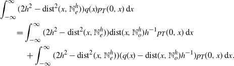(4.11) \begin{align} & \int_{-\infty}^{\infty} ({2h^2 - {\textrm{dist}}^2(x,{\mathbb{N}}^h_e)})q(x) p_T(0,x)\,{\mathrm{d}} x \notag\\ &\qquad = \int_{-\infty}^{\infty} ({2h^2 - {\textrm{dist}}^2(x,{\mathbb{N}}^h_e)}) {\textrm{dist}}(x,{\mathbb{N}}^h_o) h^{-1} p_T(0,x)\,{\mathrm{d}} x \notag\\ &\qquad\quad\, + \int_{-\infty}^{\infty} ({2h^2 - {\textrm{dist}}^2(x,{\mathbb{N}}^h_e)})(q(x)- {\textrm{dist}}(x,{\mathbb{N}}^h_o)h^{-1} ) p_T(0,x)\,{\mathrm{d}} x. \label{eqn52}\end{align}

The calculation for the first integral on the right-hand side is carried out in Reference Walsh[17]. To justify (4.1), it remains to show that the other integral behaves like ${\mathrm{O}}(h^3)$ . Since $ ({2h^2 - {\textrm{dist}}^2(x,{\mathbb{N}}^h_e)}) \le 2 h^2$ and

\[ \bigg|q(x)- \dfrac{{\textrm{dist}}(x,{\mathbb{N}}^h_o)}{h}\bigg| = \dfrac{| {\mathbb{E}}_{0,T,-x} [B_{{\mathcal{T}}(x)}] |}{h} \]

by (4.3) and (4.6), we get the desired estimate from the next corollary.

Corollary 4.1. For $T > 0$ and $h = \sqrt{T/n}$ , there exists a $C = C(T) > 0$ such that

\[ \int_{-\infty}^{\infty} | {\mathbb{E}}_{0,T,-x} [B_{{\mathcal{T}}(x)} ] | p_T(0,x) \,{\mathrm{d}} x \leq C h^2,\]

where ${\mathcal{T}}(x)$ is given in (4.6).

Proof. Since 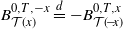$B^{0,T,-x}_{{\mathcal{T}}(x)} \stackrel{d}{=} - B^{0,T,x}_{{\mathcal{T}}(\!-\!x)}$ , it suffices to estimate the integral over $[0,\infty)$ . By (4.7),

\[| {\mathbb{E}}_{0,T,-x} [B_{{\mathcal{T}}(x)}] | \le \dfrac{{\mathbb{E}}_{0,T,-x}[ {\mathcal{T}}(x)]}{T} (2h + |x| + 3\sqrt{2 T}). \]

If $x \in (0, h)$ , then ${\mathcal{T}}(x) = {\mathcal{T}}_{(\!-\!x,h-x)}$ , and estimate (4.8) gives

\begin{align*} {\mathbb{E}}_{0,T,-x}[{\mathcal{T}}(x)] \leq 2 x \bigg({h -x+\dfrac{x}{2}}\bigg) \leq h^2. \end{align*}

For $x \ge h$ ,

\[{\mathbb{E}}_{0,T,-x}[{\mathcal{T}}(x)] \le C(T, h,-x) h^2\]

by Lemma 4.2. From the above estimates we get

(4.12) \begin{align} \int_{0}^h | {\mathbb{E}}_{0,T,-x} [B_{{\mathcal{T}}(x)}]|\, p_T(0,x) \,{\mathrm{d}} x & \leq h^2 \int_0^h \dfrac{2h + x + 3\sqrt{2T}}{T} p_T(0,x) \,{\mathrm{d}} x \leq C(T)h^2, \label{eqn53} \end{align}

and

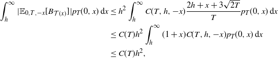(4.13) \begin{align} \int_{h}^{\infty} | {\mathbb{E}}_{0,T,-x} [B_{{\mathcal{T}}(x)}]| p_T(0,x) \,{\mathrm{d}} x &\le h^2 \int_{h}^{\infty} C(T, h,-x) \dfrac{2h + x + 3\sqrt{2T}}{T} p_T(0,x) \,{\mathrm{d}} x\nonumber\\ & \le C(T) h^2 \int_{h}^{\infty} (1+x) C(T,h,-x) p_T(0,x) \,{\mathrm{d}} x \notag \\ & \le C(T)h^2, \label{eqn54}\end{align}

where the constant C(T) varies from line to line. The last inequality in (4.13) can be seen as follows. We use the representation (3.30) for (4.9) (it is also possible to use (??) instead of (3.30)) and substitute $t=h^2 u$ , so that

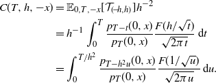\begin{align*} C(T,h,-x) &={\mathbb{E}}_{0,T,-x}[{\mathcal{T}}_{(\!-\!h,h)}] h^{-2} \\ &=h^{-1} \int_0^T \dfrac{ p_{T-t}(0,x)}{p_{T}(0,x)} \dfrac{F(h/\sqrt{t})}{\sqrt{2\pi t}} \,{\mathrm{d}} t \\ &= \int_0^{T/h^2} \dfrac{ p_{T-h^2u}(0,x)}{p_{T}(0,x)} \dfrac{F(1/\sqrt{u})}{\sqrt{2\pi u}} \,{\mathrm{d}} u. \end{align*}

By Fubini’s theorem,

\begin{align*} \int_{0}^{\infty} \dfrac{F(1/\sqrt{u})}{\sqrt{2\pi u}} \int_{h}^{\infty} (1+x) p_{T-h^2u}(0,x){{\bf 1}}_{[0,T/h^2)}(u)\,{\mathrm{d}} x \,{\mathrm{d}} u \leq C(T), \end{align*}

where for the last line we used the fact that

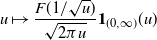\[ u \mapsto \dfrac{F(1/\sqrt{u})}{\sqrt{2\pi u}} {{\bf 1}}_{(0,\infty)}(u) \]

is a density. The claim then follows by (4.12) and (4.13).