2. Anticipative Markov modulated market

As a general setup, we assume that we work in a probability space $(\Omega, \mathcal{F},\mathbb{F},\mathbb{P})$ , where $\mathcal{F}$ is the event sigma-algebra, and $\mathbb{F}=\{\mathcal{F}_t, t\geq0\}$ is an augmented filtration that is generated by the natural filtration of the Brownian motion $W=(W_t, \, 0 \leq{t} \leq{T})$ , and let $T\gt 0$ be the horizon time.

The relation between $\mathbb{F}$ and $\mathbb{F}^\varepsilon$ is unspecified a priori. We assume that an agent can invest in a market composed just by two assets. The first one is risk-free while the second one is a risky asset; their dynamics are given by the SDEs

(2.1) \begin{align} {\mathrm{d}} P_t &= {P_t}\,r_{\varepsilon_t}\, {\mathrm{d}} t , \quad P_0 = 1, \end{align}

(2.2) \begin{align} {\mathrm{d}} S_t &= {S_t}(\eta_{\varepsilon_t}\, {\mathrm{d}} t + \xi_{\varepsilon_t}\, {\mathrm{d}} W_t) ,\quad S_0 = s_0 \gt 0 ,\end{align}

where we are considering the case that the drift, the volatility, and the short interest rate can take only two different values, i.e. $\{\eta_0,\eta_1\}$ , $\{\xi_0,\xi_1\}$ , and $\{r_0,r_1\}$ . We assume that $\xi_0,\,\xi_1,\,r_0,\,r_1\gt 0$ and $\xi_0\neq\xi_1$ . By applying a version of the Itô lemma, we obtain

\[ \ln \dfrac{S_t}{s_0} = \int_0^t \biggl( \eta_{\varepsilon_s}-\dfrac{1}{2}\xi_{\varepsilon_s} \biggr) \,{\mathrm{d}} s +\int_0^t \xi_{\varepsilon_s}\,{\mathrm{d}} W_s ,\quad 0\leq t\leq T .\]

In this case the stochastic integral is not well-defined for any possible $\mathbb{F}^\varepsilon$ , so we need to give the correct interpretation of the stochastic integral according to the measurability assumptions on $\varepsilon$ . We consider the following possibilities.

1. (a) $\mathbb{F}^\varepsilon\subset\mathbb{F}$ . In this case the classical Itô integral is well-defined and we recover a modulated version of the Merton problem, solved in [Reference Bauerle and Rieder8].

2. (b) $\varepsilon\perp W$ . The independence of the processes guarantees that the classical Itô integral is well-defined (see Section 3.3 of [Reference Øksendal29]), but the new source of randomness creates incompleteness. This problem can be considered as a special case of [Reference Karatzas, Lehoczky, Shreve and Xu26] and it has been partially solved in [Reference Ghosh, Goswami and Kumar18] and [Reference Sotomayor and Cadenillas33].

3. (c) $\varepsilon_t\in\mathcal{F}_T$ but $\varepsilon_t\not\in\mathcal{F}_t$ . In this case the process $\varepsilon$ is anticipative and the Itô integral may be not well-defined. Usually in the literature the problem is solved by applying one of the following approaches.

   1. (i) Enlargement of filtrations. We need to derive the semimartingale decomposition of W within the bigger filtration $\mathbb{G}\,:\!=\, \mathbb{F}\vee\mathbb{F}^\varepsilon$ by imposing the so-called Jacod’s hypothesis.

   2. (ii) Anticipative calculus. We extend the framework of the integral to eliminate the need for measurability assumptions. The new types of integrals considered are the forward integral and the Skorokhod integral.

4. (d) $\varepsilon_t\in\mathcal{G}_T\supsetneq\mathcal{F}_T$ but $\varepsilon_t\not\in\mathcal{F}_t$ . The anticipative issue still holds and in addition it is possible that the market is incomplete.

In this paper we solve the problems formulated in (c) and (d) in Sections 3 and 4, respectively. As we will explain, we exploit the properties of the binary state space E by using the enlargement of filtration techniques.

If we let $X^\pi=(X^\pi_t, \, 0 \leq{t} \leq{T})$ denote the wealth of the portfolio of the investor under an admissible strategy $\pi$ , we can write its dynamics as the solution of the following SDE, for $0 \leq t \leq T$ :

\begin{align*}\dfrac{{\mathrm{d}} X_t^{\pi}}{X_t^{\pi}} &= (1-\pi_t)\dfrac{{\mathrm{d}} P_t}{P_t} + \pi_t \dfrac{{\mathrm{d}} S_t}{S_t} ,\quad X_0=x_0 \gt 0 .\end{align*}

Using (2.1), it can be expressed in the following form:

(2.3) \begin{align}{\mathrm{d}} X_t^{\pi} &= (1-\pi_t)X_t^{\pi}r_{\varepsilon_t} \, {\mathrm{d}} t + \pi_t X_t^{\pi}(\eta_{\varepsilon_t} \, {\mathrm{d}} t + \xi_{\varepsilon_t} \, {\mathrm{d}} W_t) ,\quad X_0 = x_0 \gt 0 .\end{align}

Usually it is assumed that the strategy $\pi$ makes optimal use of all information at disposal of the agent at each instant, and in general we are going to assume that the agent’s flow of information, modeled by the filtration $\mathbb{H}=\{\mathcal{H}_t, 0\leq t \leq T\}$ , is possibly larger than filtration $\mathbb{F}$ , i.e. $\mathbb{F} \subset \mathbb{H}$ .

where $\pi_t$ is the proportion of the capital invested in the risky asset at time t.

We define the optimal portfolio $\pi^\mathbb{H} = (\pi^\mathbb{H}_t, \, 0 \leq{t} \leq{T})$ as the solution of the following optimization problem:

(2.4) \begin{align}\mathbb{V}_T^{\mathbb{H}} \,:\!=\, \sup\nolimits_{\pi\in\mathcal{A}({\mathbb{H}})} \mathbb{E}[U(X^{\pi}_{T})] = \mathbb{E}\bigl[U\bigl(X^{\pi^\mathbb{H}}_{T}\bigr)\bigr] .\end{align}

(2.5a) \begin{equation} U'(0) \,:\!=\, \lim_{x\to 0^+}U'(x) = + \infty ,\end{equation}

(2.5b) \begin{equation}U'(+\infty) \,:\!=\, \lim_{x\to\infty}U'(x) = 0 .\end{equation}

We extend the value of the utility function on the negative reals by setting $U(x)=-\infty$ , for $x\lt 0$ . Under the above assumption, the utility function satisfies the relation

(2.6) \begin{equation}U(I(y)) \geq U(x) + y\,(I(y) - x) \quad \text{for all $ x\gt 0,\ y\gt 0$,}\end{equation}

where I is the (continuous, strictly decreasing) inverse of U ^′; see (4.5) in [Reference Karatzas, Lehoczky, Shreve and Xu26].

We will write $\mathbb{G}$ as the minimum filtration which is right-continuous and contains $\mathbb{F}\vee\mathbb{F}^\varepsilon$ . As we consider a discrete-time Markov chain, we assume that it jumps at the set of times $\{t_0,t_1,\ldots,t_n\}$ with $t_n=T$ . Then the enlargement $\mathbb{F}\subset\mathbb{G}= \{\mathcal{G}_t, 0\leq t \leq T\}$ is a sequence of initial enlargements given by

(2.7) \begin{equation} \mathcal{G}_t = \bigcap_{s\gt t}( \mathcal{F}_s \vee \sigma(\varepsilon_{t_0}, \varepsilon_{t_1}, \ldots, \varepsilon_{t_k}) ) ,\quad t_k \leq t \lt t_{k+1} ,\ k\lt n .\end{equation}

So we can reduce it to the framework of initial enlargements in each interval $(t_k,t_{k+1})$ . Note that, as the quadratic variation of S, $\int_0^t S_s^2\xi^2_{\varepsilon_s} \,{\mathrm{d}} s$ , can be observed by the agent, the Markov chain $\varepsilon$ is also seen because $\xi_\cdot$ is bijective. Then the natural information flow of an agent who knows about the modulation of $\varepsilon$ should be $\mathbb{G}$ and the enlargement is justified according to the model given by (2.1).

In addition, Example 2.7 of [Reference Amendinger, Imkeller and Schweizer4] ensures that the binary random variable always satisfies the following Jacod hypothesis.

Assumption 2.3. The conditional distributions $\mathbb{P}(\varepsilon_{t_k}\in\cdot\mid \mathcal{F}_t)$ for $t\in(t_k,t_{k+1})$ a.s. satisfy the following absolute continuity condition with respect to $\mathbb{P}(\varepsilon_{t_k}\in\cdot)$ :

\[\mathbb{P}(\varepsilon_{t_k}\in\cdot\mid \mathcal{F}_t) \ll \mathbb{P}(\varepsilon_{t_k}\in\cdot) .\]

This assumption ensures the existence of a family of jointly measurable processes $p^{e,k}$ defined as

\begin{equation*} p_t^{e,k} = \dfrac{\mathbb{P}( \varepsilon_{t_k} = e \mid \mathcal{F}_t)}{\mathbb{P}(\varepsilon_{t_k} = e)} , \quad e\in\{0,1\} ,\ k\in\{0,1,\ldots,n-1\} ,\ t_k\leq t\lt t_{k+1} .\end{equation*}

The crucial point of the filtration enlargement is to guarantee that the $\mathbb{F}$ -local martingales remain at least $\mathbb{G}$ -semimartingales; this is known in the literature as the ( $\mathcal{H}'$ ) hypothesis. In [Reference Jacod22, Theorem 2.5] it is proved that the former Jacod’s hypothesis implies the ( $\mathcal{H}'$ ) hypothesis. As the process $p^{e,k}=(p^{e,k}_t,t_k\leq t \lt t_{k+1})$ is an $\mathbb{F}$ -martingale for any $e\in \{0,1\}$ (see [Reference Amendinger, Imkeller and Schweizer4, Lemma 2.1]), then $\langle X,p^{e,k}\rangle^{\mathbb{F}}$ is well-defined for any $\mathbb{F}$ -local martingale X. We introduce the notation

\begin{equation*} \langle X,p^{\varepsilon_{t_k},k}\rangle_t^{\mathbb{F}}\,:\!=\, \langle X,p^{\cdot,k}\rangle_t^{\mathbb{F}}\circ \varepsilon_{t_k} ,\quad t_k\leq t \lt t_{k+1} .\end{equation*}

Proposition 2.1. Let $X=(X_t, \, 0 \leq{t} \leq{T})$ be an $\mathbb{F}$ -local martingale and let $\mathbb{G}$ be as in (2.7). Then

(2.8) \begin{equation} \widehat{X}_t = X_t - \int_{t_k}^t \dfrac{{\mathrm{d}}\langle X,p^{\varepsilon_{t_k},k}\rangle_s^\mathbb{F}}{p^{\varepsilon_{t_k},k}_{s-}} ,\quad t_k\leq t \lt t_{k+1} ,\end{equation}

is a $\mathbb{G}$ -local martingale in the interval $[t_k,t_{k+1})$ .

3. Complete market

In order to get the completeness of the market, unless the opposite is stated, in this section we assume that $\varepsilon_{t_k}\in\mathcal{F}_{t_{k+1}}$ , for any $k\lt n$ , so there is no source of randomness in the market other than the one provided by the $\mathbb{F}$ -Brownian motion W. By using Jacod’s hypothesis, we guarantee the $\mathbb{G}$ -semimartingale decomposition of W. A more explicit expression for the integral process appearing in (2.8) can be obtained in the following result. We let $D_\cdot$ denote the generalized Malliavin derivative; we refer to [Reference D’Auria, Di Nunno and Salmeron14] for details on its construction and an example of its application in an optimal portfolio problem for a defaultable risky asset.

Theorem 3.1. If we consider the enlargement defined in (2.7), the $\mathbb{G}$ -adapted process

\begin{align*} \alpha_t^\varepsilon(k) &= (\!-\!1)^{\varepsilon_{t_k}+1}\mathbb{E}\bigl[D_t \varepsilon_{t_k}\mid \mathcal{F}_t\bigr]\dfrac{\varepsilon_{t_k}-\mathbb{E}[\varepsilon_{t_k}\mid \mathcal{F}_t]}{\mathbb{V}[\varepsilon_{t_k}\mid \mathcal{F}_t]}\\ &= (2\varepsilon_{t_k}-1)\dfrac{\mathbb{E}\bigl[D_t \varepsilon_{t_k}\mid \mathcal{F}_t\bigr]}{\mathbb{V}[\varepsilon_{t_k}\mid \mathcal{F}_t]}\int_{t}^{t_{k+1}} \mathbb{E}\bigl[D_s \varepsilon_{t_k}\mid \mathcal{F}_s\bigr]\,{\mathrm{d}} W_s\end{align*}

satisfies that 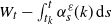$W_t - \int_{t_k}^t\alpha^\varepsilon_s(k) \,{\mathrm{d}} s$ is a $\mathbb{G}$ -Brownian motion for $t_k\leq t \lt t_{k+1}$ .

Proof. The proof follows by applying [Reference D’Auria and Salmeron13, Theorem 4.6] for binary random variables jointly with the Clark–Ocone formula (see e.g. [Reference Di Nunno, Øksendal and Proske15, Theorem 6.35])

(3.1) \begin{align} \varepsilon_{t_k} = \mathbb{E}[ \varepsilon_{t_k} ] + \int_0^{t_{k+1}} \mathbb{E}\bigl[D_t \varepsilon_{t_k}\mid \mathcal{F}_t\bigr] \,{\mathrm{d}} t ,\end{align}

where the Malliavin derivative is considered in the white noise version for any $L^2(\mathbb{P})$ -random variable that is $\mathcal{F}_T$ -measurable.

The process $\alpha^\varepsilon(k)$ is strongly related to the $\mathbb{F}$ -local martingale $p^{e,k}$ . Indeed, in [Reference Baudoin7, Remark 5] we can find the following relationship:

(3.2) \begin{equation} {\mathrm{d}} p_t^{e,k} = p_t^{e,k} \alpha_t^e(k) \,{\mathrm{d}} W_t .\end{equation}

By concatenating the previous theorem and using $\alpha^\varepsilon(k)\in L^2([t_k,t_{k+1}] \,{\mathrm{d}} t\times\mathbb{P},\mathbb{G})$ for any $k\lt n$ , we prove the following result in the whole interval time.

Corollary 3.1. In the context of Theorem 3.1,

\[ \widehat W_t \,:\!=\, W_t - \int_0^t\alpha^\varepsilon_s \,{\mathrm{d}} s ,\quad \alpha^\varepsilon_t \,:\!=\, \sum_{k=0}^{n-1}\mathbf{1}_{\{t_k\leq t \lt t_{k+1}\}}\alpha^\varepsilon_t(k) , \quad 0\leq t \leq T ,\]

is a well-defined $\mathbb{G}$ -Brownian motion in [0, T]; $\alpha^\varepsilon$ is called the information drift.

Proof. By applying Jacod’s hypothesis (see Assumption 2.3 and Theorem 3.1), we know that $\widehat W = (\widehat W_t, \, 0 \leq{t} \lt {T})$ is a $\mathbb{G}$ -Brownian motion with T excluded. Moreover, as we are considering only enlargements with purely atomic random variables, by [Reference Amendinger, Imkeller and Schweizer4, Theorem 4.1] we have

\[ \dfrac{1}{2}\int_0^T\mathbb{E}\bigl[\bigl(\alpha^\varepsilon_t\bigr)^2 \bigr]\,{\mathrm{d}} t = -\sum_{i=1}^{n-1} H(\varepsilon_{t_k}) \lt +\infty , \]

where $H(\varepsilon_{t_k})$ is the entropy operator of the random variable $\varepsilon_{t_k}$ . Then we can apply Theorem 3.2 of [Reference Imkeller20], and we deduce that $\widehat W$ is a $\mathbb{G}$ -Brownian motion with T included.

To make a consistent notation with the continuous-time processes, we sometimes consider $\varepsilon_t \,:\!=\, \varepsilon_{t_k}$ for $t_k\leq t \lt t_{k+1}$ , e.g. in the SDE of the assets. In the next lemma, following [Reference Karatzas, Lehoczky, Shreve and Xu26], we construct a $\mathbb{G}$ -exponential local martingale, usually called a deflator in the literature; see [Reference Aksamit and Jeanblanc1, Section 1.4] or [Reference Fontana16, Definition 3.1]. We will require the definition of the following process:

\begin{equation*} \theta^{\varepsilon}_t \,:\!=\, \dfrac{\eta_{\varepsilon_t} - r_{\varepsilon_t}}{\xi_{\varepsilon_t}}+\alpha_t^\varepsilon ,\quad 0 \leq t \leq T .\end{equation*}

Lemma 3.1. The process $P^{-1}ZS = (P_t^{-1}Z_tS_t,0 \leq t \leq T)$ is a non-negative $\mathbb{G}$ -local martingale, where

\begin{equation*} Z_t = \mathcal{E}_t\biggl(-\int_0^\cdot \theta^{\varepsilon}_s \,{\mathrm{d}} \widehat W_s\biggr),\end{equation*}

with $\mathcal{E}_t(\cdot)$ denoting the Doléans–Dade exponential. Moreover, $P^{-1}Z X^{\pi}$ is also a non-negative $\mathbb{G}$ -local martingale for any $\pi\in\mathcal{A}(\mathbb{G})$ .

In the following theorem we solve the utility maximization problem under the filtration $\mathbb{G}$ in a complete market modulated by $\varepsilon$ . It is one of the main results of the paper; the proof employs techniques similar to those of [Reference Amendinger, Becherer and Schweizer3], [Reference Karatzas, Lehoczky, Shreve and Xu26], and [Reference Pham and Quenez31] in the complete case.

Theorem 3.2. With a utility function satisfying Assumption 2.2, the solution of the optimal portfolio problem is

\begin{align*} \sup\nolimits_{\pi\in\mathcal{A}(\mathbb{G})} \mathbb{E}[U( X^{\pi}_T)] = \mathbb{E}[(U\circ I)(\mathcal{Y}(x_0) P_T^{-1} Z_T)] ,\end{align*}

where $X^\pi$ satisfies (2.3), I is the inverse of U^′, and $\mathcal{Y}(x_0)$ is the measurable function satisfying

\begin{equation*} \mathbb{E}[ P_T^{-1} Z_T I( \mathcal{Y}(x_0) P_T^{-1} Z_T)] = x_0 .\end{equation*}

The optimal portfolio is attained by a strategy $\pi^{\mathbb{G}}\in\mathcal{A}(\mathbb{G})$ , which hedges the random variable $X_T^{\pi^{\mathbb{G}}} = I(\mathcal{Y}(x_0) P_T^{-1} Z_T)$ .

Proof. By the completeness of the market, we know that there exists $\pi\in\mathcal{A}(\mathbb{G})$ such that $X^{\pi}_T = I(\mathcal{Y}(x_0) P_T^{-1} Z_T)$ $\mathbb{P}$ -a.s. By applying [Reference Karatzas, Lehoczky, Shreve and Xu26, Lemma 6.2], the process $P^{-1}ZX^{\pi}$ is a true $\mathbb{G}$ -martingale. Therefore, letting $X^{\widehat\pi}$ denote the wealth process for any strategy $\widehat\pi\in\mathcal{A}(\mathbb{G})$ and using the properties of the utility function (2.6), we get

\[ U\bigl(X_T^{\pi}\bigr) \geq U\bigl(X_T^{\widehat\pi}\bigr) + \mathcal{Y}(x_0)P_T^{-1}Z_T\bigl(X_t^{\pi}-X_T^{\widehat \pi}\bigr) .\]

Taking expectations on both sides, we have

\begin{align*} \mathbb{E}\bigl[ U\bigl(X_T^{\pi}\bigr)\bigr] &\geq \mathbb{E}\bigl[U\bigl(X_T^{\widehat\pi}\bigr)\bigr] + \mathbb{E}\bigl[\mathcal{Y}(x_0) P_T^{-1}Z_T \bigl(X_T^{\pi}-X_T^{\widehat \pi}\bigr)\bigr]\\ &= \mathbb{E}\bigl[U\bigl(X_T^{\widehat\pi}\bigr)\bigr] + \mathbb{E}\bigl[\mathcal{Y}(x_0) P_T^{-1}Z_T \bigl(X_T^{\pi}-X_T^{\widehat \pi}\bigr)\bigr] \\ &\geq \mathbb{E}\bigl[U\bigl(X_T^{\widehat\pi}\bigr)\bigr] + \mathcal{Y}(x_0)\bigl(x_0-\mathbb{E}\bigl[ P_T^{-1}Z_T X_T^{\widehat \pi}\bigr]\bigr)\\ & \geq \mathbb{E}\bigl[U\bigl(X_T^{\widehat\pi}\bigr)\bigr] ,\end{align*}

where in the last step we used the fact that $P^{-1} Z X^{\pi}$ and $P^{-1} ZX^{\widehat\pi}$ are respectively a $\mathbb{G}$ -martingale and a $\mathbb{G}$ -super martingale. Finally, we let $\pi^\mathbb{G}$ denote the optimal strategy.

Remark 3.1. If the information drift $\alpha^\varepsilon$ satisfies Novikov’s condition, that is,

\[ \mathbb{E}\biggl[\exp\biggl(\dfrac{1}{2} \int_0^T\bigl(\alpha^\varepsilon_t\bigr)^2 \,{\mathrm{d}} t\biggr)\biggr]\lt +\infty , \]

then (NFLVR) $_{\mathbb{G}}$ holds true and the deflator defines an equivalent local martingale measure (ELMM); see [Reference Fontana16, Proposition 3.2]. An example of enlargement satisfying this condition can be found in [Reference D’Auria and Salmeron11, Theorem 4.16]. We refer to Theorems 1.7.6.2 and 1.7.6.3 of [Reference Jeanblanc, Yor and Chesney23] for alternative sufficient criteria such as Kazamaki’s condition or the BMO criterion.

In the following result we give the additional logarithmic expected utility of an agent playing with $\mathbb{G}$ versus another who is totally unaware of the existence of such modulation.

Proposition 3.1. If we consider the enlargement $\mathbb{F}\subset\mathbb{G}$ , then the additional expected logarithmic utility is given by

\begin{align*} \mathbb{V}_T^\mathbb{G}-\mathbb{V}_T^\mathbb{F} &= (M_1+M_0)\int_0^T\mathbb{E}[D_t \varepsilon_{t}] \,{\mathrm{d}} t-\sum_{k=0}^{n-1} \sum_{e = 0}^1 \mathbb{P}(\varepsilon_{t_k}=e)\ln \mathbb{P}(\varepsilon_{t_k}=e) ,\end{align*}

where we have defined $M_e\,:\!=\, (\eta_e-r_e)/\xi_e$ , for $e\in E$ .

Proof. As $U(x) = \ln x$ , from Theorem 3.2 we conclude that

\[ X_T^{\pi^{\mathbb{G}}} = x_0P_TZ_T^{-1} ,\quad \pi^\mathbb{G}_t = \dfrac{\theta_t^\varepsilon}{\xi_{\varepsilon_t}} ,\quad 0\leq t \leq T . \]

The gains under the filtration $\mathbb{G}$ at T are

\begin{align*} \mathbb{V}_T^\mathbb{G} &= \mathbb{E}\bigl[\ln X_T^{\pi^{\mathbb{G}}}\bigr]\\ & = \ln x_0 + \int_0^T \mathbb{E}[r_{\varepsilon_t}] \,{\mathrm{d}} t + \mathbb{E}\biggl[\int_0^T \theta_t^\varepsilon \,{\mathrm{d}} \widehat W_t\biggr] + \dfrac{1}{2}\int_0^T \mathbb{E}\bigl[(\theta_t^{\varepsilon})^2\bigr]\,{\mathrm{d}} t\\ & = \ln x_0 + \int_0^T \mathbb{E}[r_{\varepsilon_t}] \,{\mathrm{d}} t + \dfrac{1}{2}\int_0^T \mathbb{E}\biggl[\biggl(\dfrac{\eta_{\varepsilon_t} - r_{\varepsilon_t}}{\xi_{\varepsilon_t}}\biggr)^2+\bigl(\alpha_t^\varepsilon \bigr)^2 + 2\dfrac{\eta_{\varepsilon_t} - r_{\varepsilon_t}}{\xi_{\varepsilon_t}}\alpha_t^\varepsilon \biggr]\,{\mathrm{d}} t\\ & = \mathbb{V}_T^\mathbb{F} + \dfrac{1}{2}\int_0^T \mathbb{E}\bigl[\bigl(\alpha_t^\varepsilon \bigr)^2\bigr]\,{\mathrm{d}} t +\int_0^T \mathbb{E}\biggl[\dfrac{\eta_{\varepsilon_t} - r_{\varepsilon_t}}{\xi_{\varepsilon_t}}\alpha_t^\varepsilon \biggr]\,{\mathrm{d}} t ,\end{align*}

where we used the fact that $\theta^\varepsilon\in L^2({\mathrm{d}} t\times\mathbb{P},\mathbb{G})$ in order to conclude the zero expectation of the Itô integral. In order to rewrite the last term, we consider

\[\dfrac{\eta_{\varepsilon_t}-r_{\varepsilon_t}}{\xi_{\varepsilon_t}} = (M_1-M_0)\varepsilon_{t_k} + M_0 ,\quad t_k\leq t \lt t_{k+1} ,\]

with the previous definition of $M_1,M_0$ . Then we get

where in the third equality we use Theorem 3.1, in the fourth one we use the fact that

\[ (M_1-M_0)\varepsilon_{t_k}(2\varepsilon_{t_k}-1) = (M_1+M_0)\varepsilon_{t_k} - M_0, \]

and by the martingale property we eliminate the $-M_0$ -term. In the fifth equality we use (3.1) and in the eighth we use

\begin{align*} \mathbb{V}[\varepsilon_{t_k}\mid \mathcal{F}_t] &= \mathbb{E}[(\varepsilon_{t_k}-\mathbb{E}[\varepsilon_{t_k}\mid \mathcal{F}_t])^2\mid \mathcal{F}_t]\\ &= \mathbb{E}\biggl[\biggl( \int_{t}^{t_{k+1}} \mathbb{E}[D_s \varepsilon_{t_k}\mid \mathcal{F}_s]\,{\mathrm{d}} W_s \biggr)^2\mid \mathcal{F}_t\biggr]\\ &= \mathbb{E}\biggl[ \int_{t}^{t_{k+1}}( \mathbb{E}[D_s \varepsilon_{t_k}\mid \mathcal{F}_s])^2 \,{\mathrm{d}} s\mid \mathcal{F}_t\biggr] .\end{align*}

The rest of the equalities use basic Itô integral properties. Finally, we compute

\begin{align*} \mathbb{E}\bigl[\bigl(\alpha_t^\varepsilon \bigr)^2\bigr] &= \mathbb{E}\Biggl[\Biggl(\sum_{k=0}^{n-1}\mathbf{1}_{\{t_k\leq t \lt t_{k+1}\}}\alpha^\varepsilon_t(k) \Biggr)^2\Biggr] = \sum_{k=0}^{n-1}\mathbf{1}_{\{t_k\leq t \lt t_{k+1}\}}\mathbb{E}\bigl[\bigl(\alpha^\varepsilon_t(k) \bigr)^2\bigr],\end{align*}

and by applying [Reference Amendinger, Imkeller and Schweizer4, Theorem 4.1], we get the result.

Remark 3.2. Although we assume that $\varepsilon$ must be $\mathcal{F}_T$ -measurable in order to use the Clark–Ocone formula (3.1), in [Reference Fontana17] it was shown that the predictable representation holds in initially enlarged filtrations satisfying Jacod’s hypothesis, so it can be trivially extended to these filtrations by considering the non-anticipative derivative instead of the process $\mathbb{E}[D_t\varepsilon_t\mid \mathcal{F}_t]$ and taking the $\mathcal{F}_t$ -conditional version of [Reference Fontana17, Theorem 2.6]. By using [Reference D’Auria and Salmeron13, Lemma 4.5], the representation

\[ \int_0^T\mathbb{E}[D_t \varepsilon_{t}] \,{\mathrm{d}} t = \sum_{k=0}^{n-1}\mathbb{P}(\varepsilon_{t_k}=1) \int_{t_k}^{t_{k+1}} \mathbb{E}\bigl[\alpha^\varepsilon_t(k)p_t^{\varepsilon,k}\bigr] \,{\mathrm{d}} t \]

also holds.

Proposition 3.2. The optimal strategy $\pi^\mathbb{G}$ , which solves problem (2.4) under logarithmic utility, i.e. $U(x) = \ln x$ , and information flow $\mathbb{G}$ , is given by

(3.3) \begin{equation} \pi^\mathbb{G}_t = \dfrac{\eta_{\varepsilon_t}-r_{\varepsilon_t}}{\xi^2_{\varepsilon_t}} +\dfrac{\alpha^{\varepsilon}_t}{\xi_{\varepsilon_t}} = \sum_{k=0}^{n-1}\mathbf{1}_{\{k\leq t \lt k+1\}}\biggl( \dfrac{\eta_{\varepsilon_{t_k}}-r_{\varepsilon_{t_k}}}{\xi^2_{\varepsilon_{t_k}}} +\dfrac{\alpha^{\varepsilon}_{t_k}(k)}{\xi_{\varepsilon_{t_k}}} \biggr) . \end{equation}

Proof. By applying the Itô lemma to (2.3), we obtain

\[\ln X_T^\pi = \ln x_0 + \int_0^T r_{\varepsilon_s} + \pi_s\biggl(\eta_{\varepsilon_k} - r_{\varepsilon_s} + \xi_{\varepsilon_s}\alpha^\varepsilon_s - \dfrac{1}{2}\xi^2_{\varepsilon_s} \pi_s \biggr) \,{\mathrm{d}} s + \int_0^T \xi_{\varepsilon_s}\pi_s \,{\mathrm{d}} \widehat W_s . \]

As $\widehat W$ is a $\mathbb{G}$ -Brownian motion, the expectation of the utility is reduced to

\[\mathbb{E}\bigl[\ln X_T^\pi\bigr] = \ln x_0 + \int_0^T \mathbb{E}\biggl[r_{\varepsilon_s} + \pi_s\biggl(\eta_{\varepsilon_k} - r_{\varepsilon_s} + \xi_{\varepsilon_s}\alpha^\varepsilon_s - \dfrac{1}{2}\xi^2_{\varepsilon_s} \pi_s \biggr) \biggr] \,{\mathrm{d}} s . \]

Following the lines of [Reference Di Nunno, Øksendal and Proske15, Theorem 16.54], we maximize for each $(s,\omega)\in[0, T]\times\Omega$ the functional

\[ J(\pi) \,:\!=\, r_{\varepsilon_s} + \pi\biggl(\eta_{\varepsilon_s} - r_{\varepsilon_s} + \xi_{\varepsilon_s}\alpha^\varepsilon_s - \dfrac{1}{2}\xi^2_{\varepsilon_s} \pi \biggr) . \]

Then a stationary point of J satisfies $0 = J'(\pi) = \eta_{\varepsilon_s} - r_{\varepsilon_s} + \xi_{\varepsilon_s}\alpha^\varepsilon_s - \xi^2_{\varepsilon_s} \pi ,$ and we obtain the candidate stated in equation (3.3). Since J is concave, the strategy $\pi^\mathbb{G}$ is a maximum of the optimization problem.

Proposition 3.3. The optimal strategy $\pi^\mathbb{G}$ which solves problem (2.4) under CRRA utility, i.e. $U(x) = x^\gamma/\gamma$ with $\gamma \in (0,1)$ , and information flow $\mathbb{G}$ , is given by

(3.4) \begin{equation} \pi^\mathbb{G}_t = \dfrac{\eta_{\varepsilon_t}-r_{\varepsilon_t}}{\xi^2_{\varepsilon_t}} +\dfrac{\alpha^{\varepsilon}_t + \rho_t}{\xi_{\varepsilon_t}} = \sum_{k=0}^{n-1}\mathbf{1}_{\{k\leq t \lt k+1\}}\biggl( \dfrac{\eta_{\varepsilon_{t_k}}-r_{\varepsilon_{t_k}}}{\xi^2_{\varepsilon_{t_k}}} +\dfrac{\alpha^{\varepsilon}_{t_k}(k) + \rho_t}{\xi_{\varepsilon_{t_k}}} \biggr) , \end{equation}

where $\rho$ is the non-anticipative derivative of $M_t \,:\!=\, \mathbb{E}\bigl[ H_T^{{{\gamma}/{(\gamma-1)}}} \mid \mathcal{G}_t \bigr]$ .

Proof. Define the process $H \,:\!=\, P^{-1}Z = (P^{-1}_tZ_t,\, 0\leq t \leq T)$ . From Theorem 3.2, we get $I(y) = y^{{{1}/{(\gamma-1)}}}$ and

\[\mathcal{Y}(x_0) = \bigl(x_0/\mathbb{E}\bigl[H_T^{{{\gamma}/{(\gamma - 1)}}}\bigr]\bigr)^{\gamma - 1},\]

and therefore

\[ X_T^{\pi^\mathbb{G}}= I(\mathcal{Y}(x_0) H_T)= x_0 \, \dfrac{H_T^{{{1}/{(\gamma-1)}}}}{\mathbb{E}\bigl[ H_T^{{{\gamma}/{(\gamma-1)}}} \bigr]} .\]

By the martingale property of $HX^{\pi^\mathbb{G}}$ ,

\begin{align*} X_t^{\pi^\mathbb{G}} &= \dfrac{1}{H_t}\mathbb{E}\bigl[H_TX_T^{\pi^\mathbb{G}} \mid \mathcal{G}_t \bigr] = \dfrac{1}{H_t} \dfrac{x_0}{M_0} \, \mathbb{E}\bigl[ H_T^{{{\gamma}/{(\gamma-1)}}} \mid \mathcal{G}_t \bigr] =\dfrac{x_0}{M_0} \dfrac{M_t}{H_t} ,\end{align*}

where we have defined $M_t \,:\!=\, \mathbb{E}\bigl[ H_T^{{{\gamma}/{(\gamma-1)}}} \mid \mathcal{G}_t \bigr]$ , and so $M_0 = \mathbb{E}\bigl[ H_T^{{{\gamma}/{(\gamma-1)}}} \bigr].$ Since $M_t$ is a $\mathbb{G}$ -martingale, and using Theorem 2.6 in [Reference Fontana17], there exists $\rho = (\rho_t, \, 0 \leq{t} \leq{T})$ adapted such that $ {\mathrm{d}} M_t = M_t \rho_t \, {\mathrm{d}} \widehat{W}_t.$ Applying the Itô lemma to $\log M_t$ , we obtain

\[ {\mathrm{d}} \log M_t = \rho_t \, {\mathrm{d}} \widehat{W}_t - \dfrac{1}{2} \rho_t^2 \, {\mathrm{d}} t . \]

Consider the process $Y = M/H = (M_t/H_t,\, 0\leq t \leq T)$ and compute its dynamics as follows:

\begin{align*} {\mathrm{d}} \log Y_t &= {\mathrm{d}} \log M_t - {\mathrm{d}} \log H_t \\ &= \biggl( \rho_t {\mathrm{d}} \widehat{W}_t - \frac{1}{2}\rho_t^2 {\mathrm{d}} t \biggr) - \biggl( -\biggl( r_t + \dfrac{1}{2}\bigl(\theta^{\varepsilon}_t\bigr)^2 \biggr) \,{\mathrm{d}} t - \theta^\varepsilon_t \,{\mathrm{d}} \widehat{W}_t \biggr)\\ &= \biggl( r_t + \frac{1}{2}\bigl(\theta^{\varepsilon}_t\bigr)^2 - \dfrac{1}{2}\rho_t^2 \biggr) \,{\mathrm{d}} t + \bigl( \rho_t + \theta^\varepsilon_t \bigr) \,{\mathrm{d}} \widehat{W}_t .\end{align*}

So we conclude that the quadratic variation of $\log Y$ is ${\mathrm{d}}\langle \log Y\rangle_t = (\rho_t + \theta^\varepsilon_t)^2 {\mathrm{d}} t$ , and

\[ \dfrac{{\mathrm{d}} Y_t}{Y_t} = {\mathrm{d}} \log Y_t + \dfrac{1}{2} {\mathrm{d}}\langle \log Y\rangle_t = \bigl( r_t + \bigl(\theta^\varepsilon_t\bigr)^2 + \rho_t\theta^\varepsilon_t \bigr) \,{\mathrm{d}} t + \bigl( \rho_t + \theta^\varepsilon_t \bigr) \,{\mathrm{d}} \widehat{W}_t .\]

Since $X_t^{\pi^\mathbb{G}} = \dfrac{x_0}{M_0} Y_t$ ,

(3.5) \begin{equation}\dfrac{{\mathrm{d}} X_t^{\pi^\mathbb{G}}}{X_t^{\pi^\mathbb{G}}} =\bigl( r_t + \bigl(\theta^{\varepsilon}_t\bigr)^2 + \rho_t\theta^\varepsilon_t \bigr) \,{\mathrm{d}} t + \bigl( \rho_t + \theta^\varepsilon_t \bigr) \,{\mathrm{d}} \widehat{W}_t .\end{equation}

Comparing with the wealth dynamics given in (2.3), written in the reference filtration $\mathbb{G}$ according to Corollary 3.1, and matching the coefficient of ${\mathrm{d}} \widehat{W}_t$ , we conclude that $\pi_t^\mathbb{G} \xi_t = \rho_t + \theta^\varepsilon_t$ and therefore we get (3.4). We only need to verify that the drift coefficient matches too. Indeed, from (2.3) we have

\begin{align*}\bigl(1-\pi_t^\mathbb{G}\bigr)r_t+\pi_t^\mathbb{G} \eta_t + \pi_t^\mathbb{G} \xi_t \alpha_t^\varepsilon&= r_t + \biggl( \dfrac{\rho_t}{\xi_t} + \dfrac{\eta_t + \xi_t\alpha_t^\varepsilon - r_t}{\xi_t^2} \biggr)(\eta_t + \xi_t\alpha_t^\varepsilon - r_t) \\ &= r_t + \rho_t \dfrac{\eta_t + \xi_t\alpha_t^\varepsilon- r_t}{\xi_t} + \dfrac{(\eta_t + \xi_t\alpha_t^\varepsilon - r_t)^2}{\xi_t^2} \\ &= r_t + \rho_t\theta^\varepsilon_t + \bigl(\theta^{\varepsilon}_t\bigr)^2 ,\end{align*}

and the last term coincides with the drift given in (3.5).

3.1. Example of increments of W

We define

\[ \varepsilon_{t_k} = \mathbf{1}_{\{W_{t_{k+1}} \gt W_{t_k}\}} ,\quad k\in\{0,1,\ldots,n-1\} .\]

Using the independent increments of W, it can be verified that $\varepsilon$ is a Markov process, and we provide an explicit expression for the information drift in the next proposition.

Proposition 3.4. We have

\[\alpha^e_t(k) \,:\!=\, \dfrac{(\!-\!1)^{1+e}}{\sqrt{t_{k+1}-t}} \dfrac{\Phi'\bigl(\frac{W_{t_k}-W_t}{\sqrt{t_{k+1}-t}}\bigr)}{\mathbb{P}(\varepsilon_{t_k} = e\mid W_t)} ,\quad e\in\{0,1\} ,\ t_k\leq t \lt t_{k+1} ,\]

where

\[\Phi(x)\,:\!=\, \int_{-\infty}^x\frac{\exp(\!-y^2/2)}{\sqrt{2\pi}}\,{\mathrm{d}} y.\]

Proof. The proof follows directly by [Reference D’Auria and Salmeron13, Proposition 4.7].

3.2. Example of running maximum of W

Let $M=(M_t, \, 0 \leq{t} \leq{T})$ be the running maximum of W, that is,

\[M_t\,:\!=\, \sup\nolimits_{0\leq s\leq t} W_s .\]

We use the Markov property of the process $M_t-W_t$ in order to define the following Markov chain $\varepsilon$ :

\begin{equation*} \varepsilon_{t_k} = \mathbf{1}_{ \{M_{t_{k+1}}-W_{t_{k+1}}\gt c \}} ,\quad c\in\mathbb{R}^+ ,\ k\in\{0,1,\ldots,n-1\} .\end{equation*}

As we have seen in Section 3.1, the optimal strategy under logarithmic utility is fully determined by the information drift $\alpha^\varepsilon$ , which is computed in the next proposition.

Proposition 3.5. We have

\[\alpha^e_t(k) \,:\!=\, \dfrac{(\!-\!1)^{1+e}}{\sqrt{t_{k+1}-t}} \dfrac{\Phi'\bigl(\frac{c+M_t-W_t}{\sqrt{t_{k+1}-t}}\bigr) - \Phi'\bigl(\frac{c-M_t+W_t}{\sqrt{t_{k+1}-t}}\bigr)}{\mathbb{P}(\varepsilon_{t_k} = e\mid \mathcal{F}_t)} ,\quad e\in\{0,1\} ,\ t_k\leq t \lt t_{k+1} . \]

Proof. We proceed as before by computing

\begin{equation*} p_t^{1,k} = \dfrac{\mathbb{P}(M_{t_{k+1}}-W_{t_{k+1}} \gt c \mid \mathcal{F}_t)}{\mathbb{P}(M_{t_{k+1}}- W_{t_{k+1}} \gt c)} . \end{equation*}

We study the numerator separately, looking for a more explicit expression. We denote $M_{s,t}\,:\!=\, \sup_{u\in[s,t]} W_u$ and $a\vee b\,:\!=\, \max\{a,b\}$ , so that

\begin{align*}& \mathbb{P}(M_{t_{k+1}}- W_{t_{k+1}} \gt c \mid \mathcal{F}_t)\\ &\quad = \mathbb{P}(M_t\vee M_{t,t_{k+1}}\, -W_{t_{k+1}} \gt c \mid \mathcal{F}_t)\\ &\quad = \mathbb{P}(M_t-W_{t_{k+1}} \gt c ,\, M_t\gt M_{t,t_{k+1}}\mid \mathcal{F}_t)\\ &\quad \quad +\mathbb{P}(M_{t,t_{k+1}}-W_{t_{k+1}} \gt c ,\, M_t\leq M_{t,t_{k+1}}\mid \mathcal{F}_t)\\ &\quad = \mathbb{P}(M_t-W_t-(W_{t_{k+1}}-W_t) \gt c ,\, M_t-W_t\gt M_{t,t_{k+1}}-W_t\mid \mathcal{F}_t)\\ &\quad \quad +\mathbb{P}(M_{t,t_{k+1}}-W_t-(W_{t_{k+1}}-W_t) \gt c ,\, M_t-W_t\leq M_{t,t_{k+1}}-W_t\mid \mathcal{F}_t)\\ &\quad = \mathbb{P}(M_t-W_t-(W_{t_{k+1}}-W_t) \gt c ,\, M_t-W_t\gt M_{t,t_{k+1}}-W_t)\\ &\quad \quad +\mathbb{P}(M_{t,t_{k+1}}-W_t-(W_{t_{k+1}}-W_t) \gt c ,\, M_t-W_t\leq M_{t,t_{k+1}}-W_t) . \end{align*}

We define $K_t=M_t-W_t$ , $X=M_{t,t_{k+1}}-W_t$ , and $Y=W_{t_{k+1}}-W_t$ . In [Reference Karatzas and Shreve25, Proposition 8.1] it is stated that the vector (X, Y) has the following density function:

\[p(x,y,t_{k+1}-t) =\dfrac{2(2x-y)}{\sqrt{2\pi(t_{k+1}-t)^3}} \exp\biggl(-\dfrac{(2x-y)^2}{2(t_{k+1}-t)}\biggr) ,\quad x\gt y\vee 0 . \]

Then

\begin{align*}& \mathbb{P}(M_{t_{k+1}}-W_{t_{k+1}} \gt c \mid \mathcal{F}_t)\\ &\quad = \mathbb{P}(Y \lt {K_t}-c ,\, X\lt{K_t}) + \mathbb{P}(X-Y \gt c ,\, X\geq {K_t})\\ &\quad =\int_0^{K_t}\int_{-\infty}^{{K_t}-c} p(x,y,t_{k+1}-t) \,{\mathrm{d}} y \,{\mathrm{d}} x + \int_{K_t}^{+\infty}\int_{-\infty}^{x-c} p(x,y,t_{k+1}-t) \,{\mathrm{d}} y \,{\mathrm{d}} x\\ &\quad = 2\int_0^{K_t} \dfrac{\Phi'\bigl( \frac{2x-{K_t}+c}{\sqrt{t_{k+1}-t}} \bigr)}{\sqrt{t_{k+1}-t}} \,{\mathrm{d}} x+ 2\int_{K_t}^{+\infty}\dfrac{\Phi'\bigl( \frac{x+c}{\sqrt{t_{k+1}-t}} \bigr)}{\sqrt{t_{k+1}-t}} \,{\mathrm{d}} x \end{align*}

\begin{align*}&\quad = \int_{c-K_t}^{c+K_t} \dfrac{\Phi'\bigl( \frac{z}{\sqrt{t_{k+1}-t}} \bigr)}{\sqrt{t_{k+1}-t}} \,{\mathrm{d}} z+ 2\int_{c+K_t}^{+\infty}\dfrac{\Phi'\bigl( \frac{z}{\sqrt{t_{k+1}-t}} \bigr)}{\sqrt{t_{k+1}-t}} \,{\mathrm{d}} z \\ &\quad = \overline{\Phi}\biggl(\dfrac{c-K_t}{\sqrt{t_{k+1}-t}}\biggr) + \overline{\Phi}\biggl(\dfrac{c+K_t}{\sqrt{t_{k+1}-t}}\biggr) . \end{align*}

By defining $f(t,K_t)\,:\!=\, \mathbb{P}(M_{t_{k+1}}-W_{t_{k+1}} \gt c \mid \mathcal{F}_t)$ , we aim to compute ${\mathrm{d}} f(t,K_t)$ via the Itô lemma. We note that the partial derivatives satisfy

\begin{align*} \dfrac{\partial}{\partial K} \, f(t,K_t) &= \dfrac{1}{\sqrt{t_{k+1}-t}}\Phi'\biggl(\dfrac{c-K_t}{\sqrt{t_{k+1}-t}}\biggr) -\dfrac{1}{\sqrt{t_{k+1}-t}}\Phi'\biggl(\dfrac{c+K_t}{\sqrt{t_{k+1}-t}}\biggr)\\* 0 &= \dfrac{\partial}{\partial t} \, f(t,K_t)+\dfrac{1}{2} \dfrac{\partial^2}{\partial K^2}f(t,K_t) , \end{align*}

and we conclude that

\[ {\mathrm{d}} f(t,K_t) = \dfrac{\partial}{\partial K} \, f(t,K_t) \,{\mathrm{d}} K_t .\]

Note that the process M is increasing only in the set $\{t,\,K_t = 0\}$ , and then we get

\[\frac{\partial}{\partial K} \, f(t,0)\,{\mathrm{d}} M_t = 0.\]

We have proved the following relationship:

\[ {\mathrm{d}} f(t,K_t) = - \dfrac{\partial}{\partial K} \, f(t,K_t) \,{\mathrm{d}} W_t = \dfrac{\Phi'\bigl(\frac{c+K_t}{\sqrt{t_{k+1}-t}}\bigr) - \Phi'\bigl(\frac{c-K_t}{\sqrt{t_{k+1}-t}}\bigr)}{\sqrt{t_{k+1}-t}} \,{\mathrm{d}} W_t . \]

We conclude that

\[ {\mathrm{d}} p_t^{1,k} = p_t^{1,k} \dfrac{\Phi'\bigl(\frac{c+K_t}{\sqrt{t_{k+1}-t}}\bigr) - \Phi'\bigl(\frac{c-K_t}{\sqrt{t_{k+1}-t}}\bigr)}{\sqrt{t_{k+1}-t}\,\mathbb{P}(\varepsilon_{t_k} = 1 \mid \mathcal{F}_t)} \,{\mathrm{d}} W_t \]

and by using (3.2) the result follows when $e=1$ . We repeat the same reasoning when $e=0$ .

3.3. Example with a path-barrier

We consider the enlargement given by the Markov chain

\[ \varepsilon_{t_k} = \mathbf{1}_{\{W_s\leq B_k\, ,\, t_k\leq s \lt t_{k+1}\}} ,\quad k\in\{0,1,\ldots,n-1 \} .\]

We assume that $B_k$ is $\mathcal{F}_{t_k}$ -measurable and it can be different for any k. Then the random variables $\{\varepsilon_{t_k}\}_k$ are independent. This example was introduced in [Reference Baudoin7, Section 3.3], under the name pathwise conditioning.

Proposition 3.6. We have

\[\alpha_t^\varepsilon(k) \,:\!=\, \left\{ \begin{aligned}& -f_{t,t_{k+1}}(B_k) \dfrac{\varepsilon_{t_k}-\mathbb{P}(\varepsilon_{t_k}=1\mid \mathcal{F}_t)} {\mathbb{P}(\varepsilon_{t_k}=1\mid \mathcal{F}_t)\mathbb{P}(\varepsilon_{t_k}=0\mid \mathcal{F}_t)}\ & if\ M_{t_k,t}\leq B_k, \\& 0 & if \ M_{t_k,t} \gt B_k, \end{aligned} \right. \]

where we compute $\mathbb{P}(\varepsilon_{t_k}=0\mid \mathcal{F}_t) = 1 - \mathbb{P}(\varepsilon_{t_k}=1\mid \mathcal{F}_t)$ and

\begin{align*} f_{t,t_{k+1}}(m) &= \dfrac{2}{ \sqrt{t_{k+1}-t}}\Phi'\biggl(\dfrac{m-W_t}{\sqrt{t_{k+1}-t}}\biggr) ,\quad m\geq W_t\\ \mathbb{P}(\varepsilon_{t_k}=1\mid \mathcal{F}_t) &= \mathbf{1}_{\{M_{t_k,t}\leq B_k\}} \int_{W_t}^{B_k} f_{t,t_{k+1}}(m)\,{\mathrm{d}} m . \end{align*}

Proof. We proceed by applying Theorem 3.1. Note that $\varepsilon$ can be expressed in terms of the running maximum of W as $\varepsilon_{t_k} = \mathbf{1}_{\{M_{t_k,t_{k+1}}\leq B_k\}}$ . Then we compute the Malliavin derivative by applying [Reference Bermin9, Corollary 5.3]. As argued in Example 5.3 of [Reference Bermin9], we have

\begin{equation*} D_t \mathbf{1}_{\{M_{t_k,t_{k+1}}\leq B_k\}} = -\delta_{B_k}(M_{t_k,t_{k+1}}) \mathbf{1}_{\{ M_{t_k,t}\leq M_{t,t_{k+1}}\! \}} . \end{equation*}

Then the conditional expectation is computed as

\begin{align*} \mathbb{E}\bigl[D_t \mathbf{1}_{\{M_{t_k,t_{k+1}}\leq B_k\}}\mid \mathcal{F}_t\bigr] &= -\mathbb{E}[\delta_{B_k}(M_{t_k,t_{k+1}}) \mathbf{1}_{\{ M_{t_k,t}\leq M_{t,t_{k+1}} \}}\mid \mathcal{F}_t] \\ &= -\mathbb{E}[\delta_{B_k}(M_{t,t_{k+1}}) \mathbf{1}_{\{ M_{t_k,t}\leq M_{t,t_{k+1}} \}}\mid \mathcal{F}_t]\\ &= -\int_{M_{t_k,t}}^{+\infty} \delta_{B_k}(m) f_{t,t_{k+1}}(m)\,{\mathrm{d}} m \\ &= -\mathbf{1}_{\{M_{t_k,t}\leq B_k\}}\, f_{t,t_{k+1}}(B_k) , \end{align*}

where $f_{t,t_{k+1}}$ is the $\mathcal{F}_t$ -conditional density function of $M_{t,t_{k+1}}$ . To end the example, we compute the conditional probabilities as follows:

\begin{align*} \mathbb{P}(\varepsilon_{t_k}=1\mid \mathcal{F}_t) &= \mathbb{P}(M_{t_k,t_{k+1}}\leq B_k\mid \mathcal{F}_s) \\ &= \mathbb{P}(M_{{t_k},t}\leq B_k, M_{t,t_{k+1}}\leq B_k\mid \mathcal{F}_t)\\ &= \mathbf{1}_{\{M_{{t_k},t}\leq B_k\}}\mathbb{P}( M_{t,t_{k+1}}\leq B_k\mid \mathcal{F}_t)\\ & = \mathbf{1}_{\{M_{{t_k},t}\leq B_k\}} \int_{W_t}^{B_k} f_{t,t_{k+1}}(m) \,{\mathrm{d}} m . \end{align*}

3.4. Example of distorted financial information

We consider a sequence $L_0,L_1,\ldots,L_n$ of $\mathcal{F}_T$ -independent binary random variables with parameters $p_0,p_1,\ldots,p_n$ , and we define the Markov chain

\[ \widetilde\varepsilon_{t_k} = L_k\varepsilon_{t_k} , \quad k\in\{0,1,\ldots,n\} ,\]

where $\varepsilon_{t_k}$ is any of those specified in Sections 3.1, 3.2, and 3.3.

This example may be used to model an insider who possesses partial information about the firm’s performance in the intervals between public disclosure dates, such as the publication of official financial statements. The underlying binary Markov chain represents the evolution of the firm’s latent condition or informational state during these periods, capturing both the intrinsic uncertainty surrounding forthcoming disclosures and possible changes in the economic or operational environment in which the company operates (e.g. favorable or adverse market conditions). The presence of an underlying Markov structure reflects the fact that, although the insider has access to additional information, the timing and impact of public disclosures remain uncertain. The binary variables $\{L_k\}_k$ introduce further noise, accounting for elements beyond the insider’s control, such as imperfect knowledge of how the market will react to the information, inaccuracies in the insider’s signals, or other unobservable factors affecting price formation. In this sense, the model incorporates both informational advantage and informational imprecision. Despite these distortions, the market remains complete, as shown in [Reference Fontana17, Proposition 3.1], which allows us to explicitly analyze how anticipative, partial, or noisy information – typical of insider settings – affects asset dynamics and optimal trading strategies.

Proposition 3.7. We have

\begin{equation*} \widetilde\alpha_t^e(k)=\left\{\begin{aligned}&\dfrac{p_k}{\widetilde p_t^{\, 0,k}}\dfrac{\mathbb{P}(\varepsilon_{t_k} = 0\mid \mathcal{F}_t)}{\mathbb{P}(\, \widetilde\varepsilon_{t_k} = 1)}\alpha^0_t(k), & e = 0 , \\&\alpha_t^1(k) , & e = 1.\end{aligned}\right.\end{equation*}

Proof. We have

\begin{align*} \widetilde p_t^{1,k} &= \dfrac{\mathbb{P}(\, \widetilde\varepsilon_{t_k}= 1\mid \mathcal{F}_t)}{\mathbb{P}(\, \widetilde\varepsilon_{t_k} = 1)} \\ &= \dfrac{\mathbb{E}\bigl[\widetilde\varepsilon_{t_k}\mid \mathcal{F}_t\bigr]}{\mathbb{P}(\, \widetilde\varepsilon_{t_k} = 1)} \\ &= \dfrac{\mathbb{E}\bigl[L_k \varepsilon_{t_k} \mid \mathcal{F}_t\bigr]}{\mathbb{P}(\, \widetilde\varepsilon_{t_k} = 1)} \\ &= \dfrac{\mathbb{E}\bigl[\mathbb{E}\bigl[L_k \varepsilon_{t_k}\mid \mathcal{F}_{t_{k+1}}\bigr]\mid \mathcal{F}_t\bigr]}{\mathbb{P}(\, \widetilde\varepsilon_{t_k} = 1)}\notag \\ &= \dfrac{\mathbb{E}\bigl[\varepsilon_{t_k} \mathbb{E}[L_k ]\mid \mathcal{F}_t\bigr]}{\mathbb{P}(\, \widetilde\varepsilon_{t_k} = 1)}\\ & = p_k \dfrac{\mathbb{E}\bigl[\varepsilon_{t_k} \mid \mathcal{F}_t\bigr]}{\mathbb{P}(\, \widetilde\varepsilon_{t_k} = 1)} \\ &= p_k \dfrac{\mathbb{P}(\varepsilon_{t_k} = 1)}{\mathbb{P}(\, \widetilde\varepsilon_{t_k} = 1)}p_t^{1,k} \\ &= p_t^{1,k} , \end{align*}

We write the differential as ${\mathrm{d}}\, \widetilde p_t^{1,k} = {\mathrm{d}} p_t^{1,k} $ and we immediately have

\begin{equation*} \widetilde\alpha^1_t(k) = \alpha_t^1(k) . \end{equation*}

We conclude that the information of $\{\widetilde\varepsilon_{t_k} = 1\}$ is the same as in $\{\varepsilon_{t_k} = 1\}$ because $\{\widetilde\varepsilon_{t_k} = 1\}\subset\{\varepsilon_{t_k} = 1\}$ . We can then argue in the same way to get $\widetilde\alpha^0_t(k)$ , and we get

\begin{align*} \widetilde p_t^{\, 0,k} &= \dfrac{\mathbb{P}(\, \widetilde\varepsilon_{t_k} = 0\mid \mathcal{F}_t)}{\mathbb{P}(\, \widetilde\varepsilon_{t_k} = 0)}\\& = \dfrac{1-\mathbb{P}(\, \widetilde\varepsilon_{t_k} = 1\mid \mathcal{F}_t)}{\mathbb{P}(\, \widetilde\varepsilon_{t_k} = 1)} \\&= \dfrac{1-p_k\mathbb{P}(\varepsilon_{t_k} = 1\mid \mathcal{F}_t)}{\mathbb{P}(\, \widetilde\varepsilon_{t_k} = 1)}\\ &= \dfrac{1-p_k+p_k\mathbb{P}(\varepsilon_{t_k} = 0\mid \mathcal{F}_t)}{\mathbb{P}(\, \widetilde\varepsilon_{t_k} = 1)}\\ & = \dfrac{1-p_k}{\mathbb{P}(\, \widetilde\varepsilon_{t_k} = 1)} +p_k\dfrac{\mathbb{P}(\varepsilon_{t_k} = 0)}{\mathbb{P}(\, \widetilde\varepsilon_{t_k} = 1)}p_t^{\, 0,k} . \end{align*}

We write the differential as

\[{\mathrm{d}}\, \widetilde p_t^{\, 0,k} = p_k\dfrac{\mathbb{P}(\varepsilon_{t_k} = 0)}{\mathbb{P}(\, \widetilde\varepsilon_{t_k} = 1)}\,{\mathrm{d}} p_t^{\, 0,k}, \]

and we conclude

\begin{align*} \dfrac{{\mathrm{d}}\, \widetilde p_t^{\, 0,k}}{\widetilde p_t^{\, 0,k}} &= p_k\dfrac{\mathbb{P}(\varepsilon_{t_k} = 0)}{\mathbb{P}(\, \widetilde\varepsilon_{t_k} = 1)}\dfrac{{\mathrm{d}} p_t^{\, 0,k}}{\widetilde p_t^{\, 0,k}}\\& = p_k\dfrac{\mathbb{P}(\varepsilon_{t_k} = 0)}{\mathbb{P}(\, \widetilde\varepsilon_{t_k} = 1)}\dfrac{ p_t^{\, 0,k}}{ \widetilde p_t^{\, 0,k}}\dfrac{{\mathrm{d}} p_t^{\, 0,k}}{ p_t^{\, 0,k}}\\& = p_k\dfrac{\mathbb{P}(\varepsilon_{t_k} = 0\mid \mathcal{F}_t)}{\mathbb{P}(\, \widetilde\varepsilon_{t_k} = 1)\widetilde p_t^{\, 0,k}}\dfrac{{\mathrm{d}} p_t^{\, 0,k}}{ p_t^{\, 0,k}} \\ &= p_k\dfrac{\mathbb{P}(\varepsilon_{t_k} = 0\mid \mathcal{F}_t)}{\mathbb{P}(\, \widetilde\varepsilon_{t_k} = 1)\widetilde p_t^{\, 0,k}}\alpha^0_t(k) \,{\mathrm{d}} W_t \\ &\,=\!:\, \widetilde\alpha^0_t(k) \,{\mathrm{d}} W_t . \end{align*}

Let $\widetilde{\mathbb{G}}$ be the filtration enlarged with the Markov chain $\widetilde\varepsilon$ . We aim to compute the additional expected logarithmic utility between $\widetilde{\mathbb{G}}$ and $\mathbb{F}$ . According to Remark 3.2, [Reference Fontana17] ensures the representation of $\widetilde\varepsilon$ , in this case as

\[\widetilde\varepsilon_{t_k} = L_k\mathbb{E}[\varepsilon_{t_k}] + \int_0^{t_{k+1}} L_k \mathbb{E}[D_t \varepsilon_{t_k}\mid \mathcal{F}_t] \,{\mathrm{d}} W_t .\]

We use [Reference Amendinger, Imkeller and Schweizer4, Theorem 4.1.1], together with Proposition 3.1, and we conclude that

\begin{align*} \mathbb{V}_T^{\widetilde{\mathbb{G}}}-\mathbb{V}_T^\mathbb{F} &= (M_1+M_0)p_k\int_0^T\mathbb{E}[D_t \varepsilon_{t}] \,{\mathrm{d}} t-\sum_{k=0}^{n-1}\sum_{e = 0}^1 \mathbb{E}[\mathbb{P}(\, \widetilde\varepsilon_{t_k}=e)\ln \mathbb{P}(\, \widetilde\varepsilon_{t_k}=e)] \\ &\quad +\sum_{k=0}^{n-1}\sum_{e = 0}^1 \mathbb{E}[\mathbb{P}(\, \widetilde\varepsilon_{t_k}=e\mid \mathcal{F}_{t_{k+1}}) \ln \mathbb{P}(\, \widetilde\varepsilon_{t_k}=e\mid \mathcal{F}_{t_{k+1}})] , \end{align*}

without assuming $\varepsilon_{t_k}\in\mathcal{F}_{t_{k+1}}$ for any $k\lt n$ . We rewrite it as

\begin{align*} \mathbb{V}_T^{\widetilde{\mathbb{G}}}- \mathbb{V}_T^\mathbb{F} &= (M_1+M_0)p_k\int_0^T\mathbb{E}[D_t \varepsilon_{t}] \,{\mathrm{d}} t -\sum_{k=0}^{n-1}\sum_{e = 0}^1 \mathbb{P}(\, \widetilde\varepsilon_{t_k}=e)\ln \mathbb{P}( \widetilde\varepsilon_{t_k} =e)\\ &\quad + \sum_{k=0}^{n-1} \mathbb{E}[ \varepsilon_{t_k} p_k \ln\!(\varepsilon_{t_k} p_k) + (1-\varepsilon_{t_k} p_k)\ln\!(1-\varepsilon_{t_k} p_k) ]\\ &= (M_1+M_0)p_k\int_0^T\mathbb{E}[D_t \varepsilon_{t}] \,{\mathrm{d}} t -\sum_{k=0}^{n-1}\sum_{e = 0}^1 \mathbb{P}(\, \widetilde\varepsilon_{t_k}=e)\ln \mathbb{P}(\, \widetilde\varepsilon_{t_k}=e) \\ &\quad +\sum_{k=0}^{n-1} \mathbb{P}(\varepsilon_{t_k}=1) ( p_k\ln p_k + (1-p_k)\ln\!(1-p_k)) . \end{align*}

Finally, we compute the additional expected logarithmic utility between $\mathbb{G}$ and $\widetilde{\mathbb{G}}$ by including $\mathbb{V}_T^\mathbb{G}-\mathbb{V}_T^{\mathbb{F}}$ given by Proposition 3.1:

\begin{align*} \mathbb{V}_T^\mathbb{G} - \mathbb{V}_T^{\widetilde{\mathbb{G}}} &= (M_1+M_0)(1-p_k)\int_0^T\mathbb{E}[D_t \varepsilon_{t}] \,{\mathrm{d}} t\\[-2pt] &\quad - \sum_{k=0}^{n-1}\sum_{e = 0}^1 ( \mathbb{P}(\varepsilon_{t_k}=e)\ln \mathbb{P}(\varepsilon_{t_k}=e) + \mathbb{P}(\, \widetilde\varepsilon_{t_k}=e)\ln \mathbb{P}( \widetilde\varepsilon_{t_k} = e) )\\[-2pt] &\quad -\sum_{k=0}^{n-1} \mathbb{P}(\, \widetilde\varepsilon_{t_k}=1) ( p_k\ln p_k + (1-p_k)\ln\!(1-p_k)) . \end{align*}

4. Incomplete market

In this section we assume that the Markov chain $\varepsilon$ that modulates the market is measurable in a sigma-algebra bigger than $\mathcal{F}_T$ . In particular, the market coefficients are also modulated by a Brownian motion $B=(B_t, \, 0 \leq{t} \leq{T})$ as follows:

\begin{align*} {\mathrm{d}} P_t &= {P_t}\,r_{\varepsilon_t}(B_{\cdot})\, {\mathrm{d}} t , \quad P_0 = 1 \\ {\mathrm{d}} S_t &= {S_t}(\eta_{\varepsilon_t}(B_{\cdot})\, {\mathrm{d}} t + \xi_{\varepsilon_t}(B_{\cdot})\, {\mathrm{d}} W_t) ,\quad S_0 = s_0 \gt 0 .\end{align*}

We assume that W and B are $\mathbb{P}$ -independent and we introduce the natural information flow $\mathbb{E} = \{\mathcal{E}_t, t\geq0\}$ induced by W and B as

\[\mathcal{E}_t = \sigma( (W_s,B_s), 0\leq s \leq t ) .\]

Note that (W, B) has the predictable representation property in the sense that any $(\mathbb{P},\mathbb{E})$ -local martingale $m=(m_t, \, 0 \leq{t} \leq{T})$ can be written as

(4.1) \begin{equation} m_t = m_0 + \int_0^t \varphi_s{\mathrm{d}} W_s + \int_0^t \phi_s {\mathrm{d}} B_s ,\end{equation}

where $\varphi$ , $\phi$ are square-integrable $\mathbb{E}$ -predictable processes. Indeed, for any $F\in\mathcal{E}_T$ -measurable random variable satisfying $F\in L^2(\mathbb{P})$ , the following representation holds:

(4.2) \begin{equation} F = \mathbb{E}[F] + \int_0^T\mathbb{E}[D^{(1)}_sF\mid \mathcal{E}_s] \,{\mathrm{d}} W_s + \int_0^T\mathbb{E}[D^{(2)}_s F\mid \mathcal{E}_s] \,{\mathrm{d}} B_s ,\end{equation}

where $D^{(1)}$ and $D^{(2)}$ represent the Malliavin derivative with respect to W and B respectively; see [Reference Di Nunno, Øksendal and Proske15, Theorem 13.28] for a reference. In this case the discrete time Markov chain satisfies that $\varepsilon_{t_k}$ is $\mathcal{E}_{t_{k+1}}$ -measurable, where $\mathbb{G}$ is the same enlargement as in (2.7). As we maintain the binary state space, Jacod’s hypothesis is still satisfied within the filtration $\mathbb{E}$ . The motivation is given by assuming the existence of an additional source of uncertainty in the information flow. This slight modification induces incompleteness in the market and the computations of Section 3 do not hold.

Proposition 4.1. If we consider the enlargement $\mathbb{E}\subset\mathbb{G}$ , then

\begin{alignat*}{3} \widehat W_t &\,:\!=\, W_t - \int_0^t\alpha^\varepsilon_s \,{\mathrm{d}} s , \quad &\alpha^\varepsilon_t& \,:\!=\, \sum_{k=0}^{n-1}\mathbf{1}_{\{t_k\leq t \lt t_{k+1}\}}\alpha^\varepsilon_t(k) , \quad &\alpha^e_t(k)\,:\!=\, & \dfrac{\mathbb{E}\bigl[D^{(1)}_t\mathbf{1}_{\{\varepsilon_{t_k}=e\}}\mid \mathcal{E}_t\bigr]}{\mathbb{P}(\varepsilon_{t_k}=e\mid \mathcal{E}_t)},\\ \widehat B_t &\,:\!=\, B_t - \int_0^t\gamma^\varepsilon_s \,{\mathrm{d}} s , \quad &\gamma^\varepsilon_t& \,:\!=\, \sum_{k=0}^{n-1}\mathbf{1}_{\{t_k\leq t \lt t_{k+1}\}}\gamma^\varepsilon_t(k) , \quad &\gamma^e_t(k)\,:\!=\, & \dfrac{\mathbb{E}\bigl[D^{(2)}_t\mathbf{1}_{\{\varepsilon_{t_k}=e\}}\mid \mathcal{E}_t\bigr]}{\mathbb{P}(\varepsilon_{t_k}=e\mid \mathcal{E}_t)},\end{alignat*}

where $\widehat W,\,\widehat B$ are $\mathbb{G}$ -Brownian motions in [0, T].

Proof. The result directly follows from Proposition 2.1 and the representation given by (4.2). In particular, we get

\begin{align*} p_t^{e,k} &= \dfrac{\mathbb{P}(\varepsilon_{t_k}=e\mid \mathcal{E}_t)}{\mathbb{P}(\varepsilon_{t_k}=e)}\\ & = \dfrac{\mathbb{E}\bigl[\mathbf{1}_{\{\varepsilon_{t_k}=e\}}\mid \mathcal{E}_t\bigr]}{\mathbb{P}(\varepsilon_{t_k}=e)} \\ &= \dfrac{\mathbb{P}(\varepsilon_{t_k}=e) + \mathbb{E}\bigl[\int_0^T\mathbb{E}\bigl[D^{(1)}_s\mathbf{1}_{\{\varepsilon_{t_k}=e\}}\mid \mathcal{E}_s\bigr] \,{\mathrm{d}} W_s + \int_0^T\mathbb{E}\bigl[D^{(2)}_s\mathbf{1}_{\{\varepsilon_{t_k}=e\}}\mid \mathcal{E}_s\bigr] \,{\mathrm{d}} B_s \mid \mathcal{E}_t\bigr]}{\mathbb{P}(\varepsilon_{t_k}=e)}\\ &= \dfrac{\mathbb{P}(\varepsilon_{t_k}=e) + \int_0^t\mathbb{E}\bigl[D^{(1)}_s\mathbf{1}_{\{\varepsilon_{t_k}=e\}}\mid \mathcal{E}_s\bigr] \,{\mathrm{d}} W_s + \int_0^t\mathbb{E}\bigl[D^{(2)}_s\mathbf{1}_{\{\varepsilon_{t_k}=e\}}\mid \mathcal{E}_s\bigr] \,{\mathrm{d}} B_s }{\mathbb{P}(\varepsilon_{t_k}=e)} .\end{align*}

Then we write the differential form as

\[\dfrac{{\mathrm{d}} p_t^{e,k}}{p_t^{e,k}} = \dfrac{\mathbb{E}\bigl[D^{(1)}_t\mathbf{1}_{\{\varepsilon_{t_k}=e\}}\mid \mathcal{E}_t\bigr]}{\mathbb{P}(\varepsilon_{t_k}=e\mid \mathcal{E}_t)} \,{\mathrm{d}} W_t +\dfrac{\mathbb{E}\bigl[D^{(2)}_t\mathbf{1}_{\{\varepsilon_{t_k}=e\}}\mid \mathcal{E}_t\bigr] }{\mathbb{P}(\varepsilon_{t_k}=e\mid \mathcal{E}_t)} \,{\mathrm{d}} B_t , \]

and by the independence of W and B it follows that $\langle W,B\rangle_s^{\mathbb{E}} = 0$ , and we get the result.

Lemma 4.1. Let $L=(L_t, \, 0 \leq{t} \leq{T})$ be any $(\mathbb{P},\mathbb{G})$ -local martingale with $L_0 = 0$ . Then there exist square-integrable and $\mathbb{G}$ -predictable processes $\lambda$ and $\nu$ such that

\[ L_t = \int_0^t \lambda_s {\mathrm{d}} \widehat W_s + \int_0^t \nu_s {\mathrm{d}} \widehat B_s ,\quad 0 \leq t\leq T . \]

Motivated by Lemma 4.1, we introduce the exponential $(\mathbb{P},\mathbb{G})$ -local martingale

\[ Z^{\lambda,\nu}_t \,:\!=\, \exp\biggl( -\int_0^t \lambda_s {\mathrm{d}} \widehat W_s - \int_0^t \nu_s {\mathrm{d}} \widehat B_s -\dfrac{1}{2}\int_0^t \bigl(\lambda_s^2 + \nu_s^2\bigr) \,{\mathrm{d}} s \biggr) ,\quad 0 \leq t\leq T . \]

Lemma 4.2. The family of processes $\{Z^\nu\}$ with $\nu\in L^2({\mathrm{d}} t\times\mathbb{P},\mathbb{G})$ satisfies that $P^{-1}Z^\nu S$ and $P^{-1}Z^\nu X^{\pi}$ are non-negative $\mathbb{G}$ -local martingales, where we define

\[ Z^{\nu}_t \,:\!=\, \exp\biggl( -\int_0^t \theta^\varepsilon_s \,{\mathrm{d}} \widehat W_s - \int_0^t \nu_s \,{\mathrm{d}} B_s -\dfrac{1}{2}\int_0^t \bigl(\theta^\varepsilon_s\bigr)^2 + \nu_s^2\, {\mathrm{d}} s \biggr) ,\quad 0 \leq t\leq T . \]

Proof. By using Itô calculus, we get

\begin{align*} Z^{\lambda,\nu}_tP_t^{-1}S_t &= S_0\exp\biggl\{\int_0^t \biggl( \eta_s(B_\cdot) - r_s(B_\cdot) - \dfrac{1}{2}\xi_s^2(B_\cdot) + \xi_s(B_\cdot)\alpha_s^\varepsilon -\dfrac{1}{2}\bigl(\lambda_s^2+\nu_s^2\bigr)\biggr) \,{\mathrm{d}} s \\ &\quad +\int_0^t (\xi_s(B_\cdot) - \lambda_s ) \,{\mathrm{d}} \widehat W_s -\int_0^t \nu_s \,{\mathrm{d}} B_s \biggr\} ,\end{align*}

then we differentiate in the Itô sense,

\begin{align*} \dfrac{{\mathrm{d}}\bigl(Z^{\lambda,\nu}_tP_t^{-1}S_t\bigr)}{Z^{\lambda,\nu}_tP_t^{-1}S_t} &= \xi_t(B_\cdot)\biggl( \dfrac{\eta_t(B_\cdot) - r_t(B_\cdot)}{\xi_t(B_\cdot)} +\alpha_t^\varepsilon - \lambda_t\biggr) \,{\mathrm{d}} t + (\xi_t(B_\cdot) - \lambda_t ) \,{\mathrm{d}} \widehat W_t - \nu_t \,{\mathrm{d}} B_t .\end{align*}

By imposing the condition that the drift part is null, we obtain $\lambda_t=\theta^\varepsilon_t$ .

The Inada conditions (2.5) ensure that the function I is such that $I(0+\!) = \infty$ and $I(\infty) = 0$ . We define

\[ \widehat U (y) \,:\!=\, \max_{x \gt 0} \{U(x) - xy\} = U(I(y)) - yI(y) ,\quad 0 \lt y \lt +\infty ,\]

and formulate some assumptions appearing in [Reference Karatzas, Lehoczky, Shreve and Xu26] (see also [Reference Pham and Quenez31]). The first one excludes logarithmic utility, but in this case the optimization problem can be solved explicitly.

So the dual problem of (2.4) is stated as follows:

(4.3) \begin{equation} \widetilde{V}(y) \,:\!=\, \inf_{\nu} \mathbb{E}\bigl[\widetilde{U}\bigl(y P_T^{-1}Z_T^\nu\bigr)\bigr] .\end{equation}

Finally, we introduce the following family of random variables:

(4.4) \begin{equation} \xi^{\nu}(x_0) \,:\!=\, I\bigl( \mathcal{Y}^\nu(x_0) P^{-1}_T Z^\nu_T \bigr) ,\quad \nu\in L^2({\mathrm{d}} t\times\mathbb{P},\mathbb{G}) ,\end{equation}

where $\mathcal{Y}^\nu(x_0)$ satisfies

(4.5) \begin{equation} \mathbb{E}\bigl[ P_T^{-1} Z^\nu_T I\bigl( \mathcal{Y}^\nu(x_0) P_T^{-1} Z^\nu_T\bigr)\bigr] = x_0 .\end{equation}

The following result, proved in [Reference Karatzas, Lehoczky, Shreve and Xu26], gives the existence of a deflator under which the contingent claim (4.4) is hedgeable and the expectation is preserved.

Proposition 4.2. Under Assumption 4.1, there exists $\lambda$ such that for any $\nu$

\begin{equation*} \mathbb{E}\bigl[P_T^{-1}Z_T^\nu \xi^{\lambda}({x_0})\bigr] \leq x_0 = \mathbb{E}\bigl[P_T^{-1}Z_T^{\lambda}\xi^{\lambda}(x_0)\bigr] .\end{equation*}

Moreover, the random variable $\xi^{\lambda}(x_0)$ is hedgeable and $\lambda$ is the solution of problem (4.3) with parameter $\mathcal{Y}^\lambda(x_0)$ .

Theorem 4.1. The solution of the optimal portfolio problem is

\begin{align*} \mathrm{ess\,sup\,}_{\pi\in\mathcal{A}(\mathbb{G})} \mathbb{E}[U( X^{\pi}_T)] = \mathbb{E}[U(\xi^\lambda(x_0))] ,\end{align*}

where $X^\pi$ satisfies (2.3). The optimal portfolio is attained by a strategy $\pi^{\mathbb{G}}\in\mathcal{A}(\mathbb{G})$ which hedges the random variable $\xi^\lambda(x_0) = I\bigl(\mathcal{Y}^\lambda(x_0) P_T^{-1} Z^\lambda_T\bigr)$ , where $\lambda$ is defined in Proposition 4.2.

Example 4.1. We define

\[ \varepsilon_{t_k} = \mathbf{1}_{\{W_{t_{k+1}} \gt W_{t_k}\}}\mathbf{1}_{\{B_{t_{k+1}} \gt B_{t_k}\}} ,\quad k\in\{0,1,\ldots,n-1\} .\]

We aim to compute the information drifts of W and B using Proposition 4.1. We proceed as follows:

\begin{align*} \alpha^1_t(k)&= \dfrac{\mathbb{E}\bigl[D^{(1)}_t\varepsilon_{t_k}\mid \mathcal{E}_t\bigr]}{\mathbb{P}(\varepsilon_{t_k}=1\mid \mathcal{E}_t)}\\ & = \dfrac{\mathbb{E}\bigl[\mathbf{1}_{\{B_{t_{k+1}} \gt B_{t_k}\}}D^{(1)}_t\mathbf{1}_{\{W_{t_{k+1}} \gt W_{t_k}\}} \mid \mathcal{E}_t\bigr]}{\mathbb{P}(\varepsilon_{t_k}=1\mid \mathcal{E}_t)}\\ &= \dfrac{\mathbb{E}\bigl[\mathbf{1}_{\{B_{t_{k+1}} \gt B_{t_k}\}}\delta_{W_{t_k}}(W_{t_{k+1}}) \mid \mathcal{E}_t\bigr]}{\mathbb{P}(\varepsilon_{t_k}=1\mid \mathcal{E}_t)}\\ & = \dfrac{\mathbb{E}\bigl[\mathbb{E}\bigl[\mathbf{1}_{\{B_{t_{k+1}} \gt B_{t_k}\}}\delta_{W_{t_k}}(W_{t_{k+1}}) \mid \mathcal{E}_t\vee\mathcal{F}_{t_{k+1}}\bigr] \mid \mathcal{E}_t\bigr]}{\mathbb{P}(\varepsilon_{t_k}=1\mid \mathcal{E}_t)} \\ &= \dfrac{\mathbb{E}\bigl[\delta_{W_{t_k}}(W_{t_{k+1}})\mathbb{E}\bigl[\mathbf{1}_{\{B_{t_{k+1}} \gt B_{t_k}\}} \mid \mathcal{E}_t\bigr]\mid \mathcal{E}_t\bigr]}{\mathbb{P}(\varepsilon_{t_k}=1\mid \mathcal{E}_t)}\\ & = \overline\Phi\biggl(\dfrac{B_{t_k}-B_t}{\sqrt{t_{k+1}-t}}\biggr)\dfrac{1}{\sqrt{t_{k+1}-t}}\dfrac{\Phi'\bigl(\frac{W_{t_k}-W_t}{\sqrt{t_{k+1}-t}}\bigr)}{\mathbb{P}(\varepsilon_{t_k}=1\mid \mathcal{E}_t)}. \end{align*}

Similarly, we compute

\begin{equation*} \gamma^1_t(k)= \dfrac{\mathbb{E}\bigl[D^{(2)}_t\varepsilon_{t_k}\mid \mathcal{E}_t\bigr]}{\mathbb{P}(\varepsilon_{t_k}=1\mid \mathcal{E}_t)} = \overline\Phi\biggl(\dfrac{W_{t_k}-W_t}{\sqrt{t_{k+1}-t}}\biggr)\dfrac{1}{\sqrt{t_{k+1}-t}}\dfrac{\Phi'\bigl(\frac{B_{t_k}-B_t}{\sqrt{t_{k+1}-t}}\bigr)}{\mathbb{P}(\varepsilon_{t_k}=1\mid \mathcal{E}_t)} .\end{equation*}

As we have pointed out, logarithmic utility does not satisfy Assumption 4.1. However, we can maximize handling with the good properties of the logarithmic utility, as in Section 3.1. We conclude that the optimal strategy is

\begin{equation*} \pi^\mathbb{G}_t = \dfrac{\eta_{\varepsilon_t}}{\xi^2_{\varepsilon_t}} +\dfrac{\alpha^{\varepsilon}_t}{\xi_{\varepsilon_t}} = \sum_{k=0}^{n-1}\mathbf{1}_{\{k\leq t \lt k+1\}}\biggl( \dfrac{\eta_{\varepsilon_{t_k}}}{\xi^2_{\varepsilon_{t_k}}} +\dfrac{\alpha^{\varepsilon}_{t_k}(k)}{\xi_{\varepsilon_{t_k}}} \biggr) ,\end{equation*}

which depends only on $\alpha^{\varepsilon}_t(k)$ and not on $\gamma^{\varepsilon}_t(k)$ .