1 Introduction
The basic model of a random graph is the Erdős–Rényi model
$G(n, p)$
 , which is a graph with vertex set
$[n]:=\{1, 2, \ldots , n\}$
 , where each edge
$(i, j)$
 is present independently with probability
$p \in [0, 1]$
 , for
$1 \leq i < j \leq n$
 . This model forms the foundation of random graph theory and network analysis, and its properties have been extensively studied. In this article, we consider multiplex networks, which consist of multiple graphs defined on a common set of nodes. In such networks, the edges of each graph (referred to as the layers of the multiplex) represent different types of interactions. For example, in social networks, the different layers can correspond to types of relationships (such as friendship, collaboration, or family ties) or modes of communication (such as email, phone, or message) [Reference Fienberg, Meyer and Wasserman14, Reference Padgett and Ansell28, Reference Pattison and Wasserman30, Reference Wasserman and Faust36]; in transportation networks, layers represent different modes of transportation [Reference Bergermann and Stoll5, Reference Cardillo, Gómez-Gardenes, Zanin, Romance, Papo, del Pozo and Boccaletti9, Reference Oliveira, Carpi and Atman27, Reference Strano, Shai, Dobson and Barthelemy35] (also known as multi-mode graphs [Reference Kirkpatrick and Williams21]); and in biological networks, such as those describing connections in the nervous system, layers may represent synaptic (chemical) or electrical links between neurons [Reference Bentley, Branicky, Barnes, Chew, Yemini, Bullmore, Vértes and Schafer4]; to name a few. The study of multiplex networks has been growing rapidly in recent years, with applications appearing across a wide range of disciplines (see the monographs [Reference Bianconi6, Reference Cozzo, De Arruda, Rodrigues and Moreno12, Reference Kiani, Gomez-Cabrero and Bianconi20] and the references therein).
A basic model of a random multiplex is the correlated Erdős–Rényi model. In this model, each layer marginally follows the classical (single layer) Erdős–Rényi model, while the edges across the layers are dependent. We define this model formally below, considering two layers for simplicity. For this, we need to introduce a few notations. A multiplex with two layers will be denoted by
$\boldsymbol {G} = (V(\boldsymbol {G}), G^{(1)}, G^{(2)})$
 , where
$V(\boldsymbol {G})$
 is the common vertex set and
$G^{(1)} = (V(\boldsymbol G), E(G^{(1)}))$
 and
$G^{(2)} = (V(\boldsymbol G), E(G^{(2)}))$
 are the two layers, which are two simple graphs with vertex set
$V(\boldsymbol G)$
 and edge sets
$E(G^{(1)})$
 and
$E(G^{(2)})$
 , respectively. The union of the edge sets across the two layers will be denoted by
$E(\boldsymbol {G})= E(G^{(1)}) \cup E(G^{(2)})$
 .
Definition 1.1 In the correlated Erdős–Rényi model, a random multiplex
$\boldsymbol G_n := ([n], G_n^{(1)}, G_n^{(2)})$
 is generated as follows: Let
$(a_{ij}^{(1)}, a_{ij}^{(2)})_{1 \leq i < j \leq n}$
 be an i.i.d. collection of pairs of correlated Bernoulli random variables distributed as

where

Then, for
$1 \leq i < j \leq n$
 , the edge
$(i,j)$
 is included in the two layers as follows:
-
• if $a_{ij}^{(1)} = 1$
 and
$a_{ij}^{(2)} = 0$
, then
$(i, j) \in E(G_n^{(1)})$
and
$(i, j) \notin E(G_n^{(2)})$
;
-
• if $a_{ij}^{(1)} = 0$
and
$a_{ij}^{(2)} = 1$
, then
$(i, j) \notin E(G_n^{(1)})$
and
$(i, j) \in E(G_n^{(2)})$
; -
• if $a_{ij}^{(1)} = a_{ij}^{(2)} = 1$
, then
$(i, j) \in E(G_n^{(1)}) \cap E(G_n^{(2)})$
; -
• if $a_{ij}^{(1)} = a_{ij}^{(2)} = 0$
, then
$(i, j) \notin E(G_n^{(1)}) \cup E(G_n^{(2)})$
.


(Note that the graphs
$G_n^{(1)}$
 and
$G_n^{(2)}$
 are marginally distributed as Erdős–Rényi models
$G(n, p_1)$
 and
$G(n, p_2)$
 , respectively, and the edges appear in both layers with probability
$p_{12}$
 .) We write
$\boldsymbol G_n\sim G(n,p_1,p_2,p_{12})$
 for a random multiplex generated as above and refer to
$G(n,p_1,p_2,p_{12})$
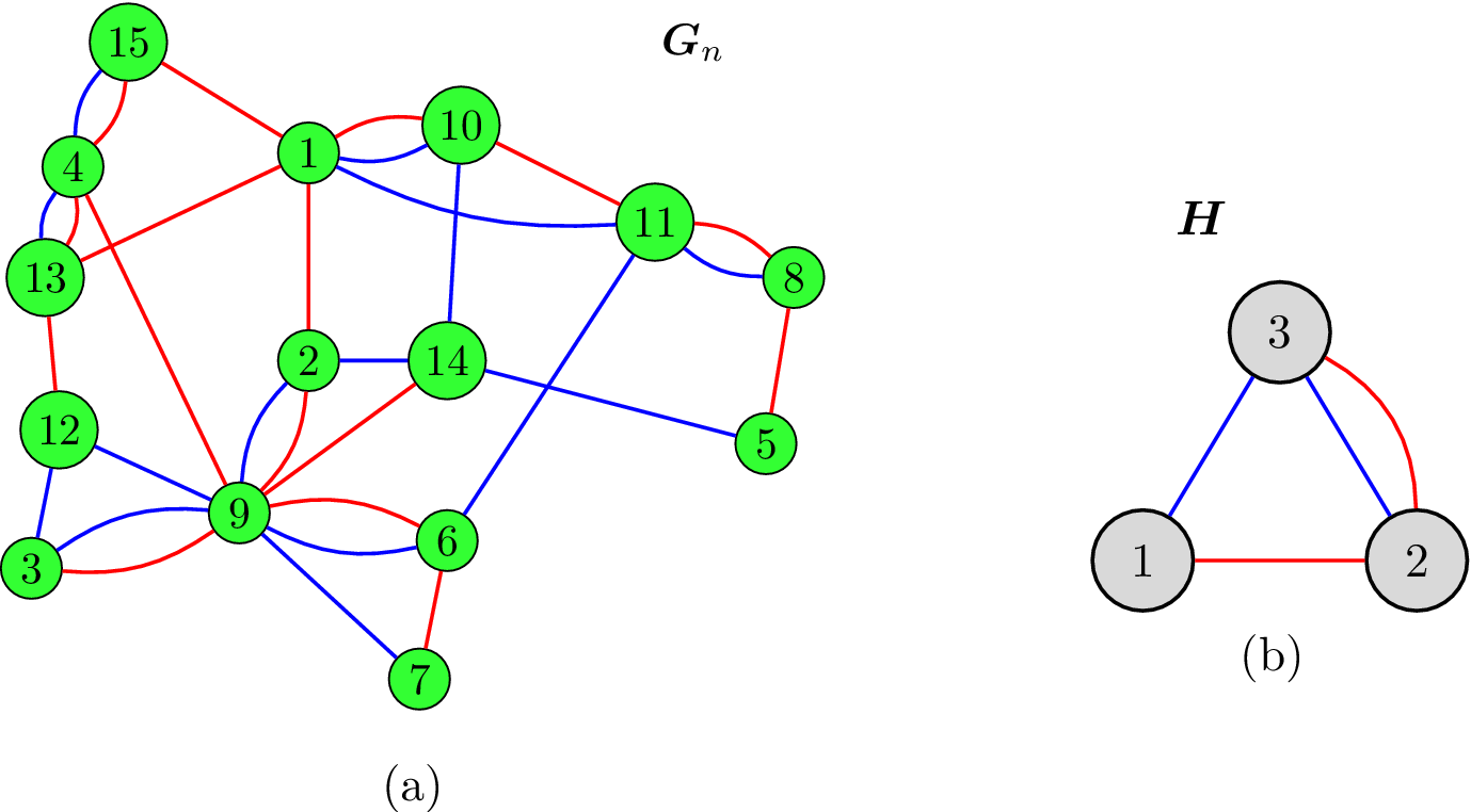
 as the correlated Erdős–Rényi multiplex model. Figure 1(a) shows a sample from the correlated Erdős–Rényi model with
$n=15$
 and
$p_1=p_2=0.15$
 ,
$p_{12}=0.05$
 .
(a) A sample
$\boldsymbol {G}_n$
 from the correlated Erdős–Rényi multiplex with
$n=15$
 and
$p_1=p_2=0.15$
 , and
$p_{12}=0.05$
 . The edges in layer
$1$
 are colored blue, while those in layer
$2$
 are colored red. (b) A fixed multiplex
$\boldsymbol {H}$
 on three vertices.
$X(\boldsymbol H, \boldsymbol G_n)$
 counts the number of copies of
$\boldsymbol H$
 in
$\boldsymbol G_n$
 (see (2.1) for the formal definition).

Figure 1 Long description
The diagram consists of two panels labeled a and b.
Panel a, labeled G sub n, displays a complex network of 15 green circular nodes numbered 1 through 15. The nodes are interconnected by two types of edges. Blue edges represent layer 1 and red edges represent layer 2. Some node pairs are connected by a single blue edge, some by a single red edge, and others by both a blue and a red edge, creating parallel curved paths between them. For example, nodes 9 and 6 are connected by both a blue and a red edge, while nodes 15 and 1 are connected only by a red edge.
Panel b, labeled H, displays a smaller triangular multiplex graph with three gray circular nodes numbered 1, 2, and 3. Node 1 is at the bottom left, node 2 is at the bottom right, and node 3 is at the top center. The connections are as follows. A single blue edge connects nodes 1 and 3. A single red edge connects nodes 1 and 2. Nodes 2 and 3 are connected by both a blue edge and a red edge.
The correlated Erdős–Rényi model initially appeared in a different guise in the context of network de-anonymization [Reference Pedarsani and Grossglauser31]. Recently, this has been adopted as the canonical model in random graph matching and related problems (see [Reference Barak, Chou, Lei, Schramm and Sheng2, Reference Huang and Yang16, Reference Lyzinski, Fishkind, Fiori, Vogelstein, Priebe and Sapiro22–Reference Mao, Wu, Xu and Yu25], among several others). In this context, a prototypical statistical question is to detect whether two networks are edge-correlated through some latent vertex correspondence. Test statistics for such problems often involve the covariance between subgraph count statistics across the two networks [Reference Barak, Chou, Lei, Schramm and Sheng2, Reference Huang and Yang16, Reference Mao, Wu, Xu and Yu25]. Analyzing these quantities requires understanding the asymptotic properties of counts of two overlapping subgraphs defined on a shared set of nodes, which naturally connects to the study of submultiplexes within a multiplex network.
Motivated by the above problems and the growing need for the multiplex framework in modeling large-scale complex systems, in this article, we aim to understand the asymptotic behavior of submultiplexes. Analogous to the role of subgraphs (motifs) in single-layer networks, submultiplexes are key local features that capture important structural properties in multiplex networks. Focusing on the correlated Erdős–Rényi model, we begin by deriving the threshold for the emergence (containment) of a fixed submultiplex
$\boldsymbol H$
 in a realization of the random multiplex
$\boldsymbol G_n \sim G(n, p_1, p_2, p_{12})$
 . Specifically, we determine the precise threshold condition under which
$X(\boldsymbol H, \boldsymbol G_n)$
 , the number of copies of
$\boldsymbol H$
 in
$\boldsymbol G_n$
 (see Section 2.1 for the formal definition and Figure 1 for an illustration), converges in probability to zero or to infinity. The threshold condition corresponds to a minimization problem that is determined by the submultiplexes of
$\boldsymbol {H}$
 with the smallest expected number of copies. By parametrizing the model so that the connection probabilities
$p_1, p_2, p_{12}$
 decay polynomially, we show that the satisfiability region, that is, the regime where
$\boldsymbol {G}_n$
 contains many copies of
$\boldsymbol H$
 , is a polyhedral subset of
$\mathbb R^3$
 . Next, we show that whenever
$\boldsymbol G_n$
 contains many copies of
$\boldsymbol H$
 , that is, for all parameter values in the satisfiability region,
$X(\boldsymbol H, \boldsymbol G_n)$
 is asymptotically normal after appropriate normalization. Additionally, our result provides an explicit convergence rate for this normal approximation in the Wasserstein distance (see Theorem 2.6). We next analyze the regime in which the parameter values lie on the boundary of the satisfiability region (the threshold surface). At such boundary points, the asymptotic behavior of
$X(\boldsymbol H, \boldsymbol G_n)$
 depends on the structure of the minimizers of the threshold condition. If the set of minimizers contains
$\boldsymbol H$
 itself (in which case, we say
$\boldsymbol H$
 is balanced for that parameter value), then the distribution of
$X(\boldsymbol H, \boldsymbol G_n)$
 depends on whether this minimizer is unique. In the strictly balanced case, where the minimizer is achieved uniquely at
$\boldsymbol H$
 , we show that
$X(\boldsymbol H, \boldsymbol G_n)$
 converges in distribution to a Poisson, under an additional nondegeneracy condition (see Theorem 2.8). On the other hand, if all minimizers occur at proper submultiplexes of
$\boldsymbol H$
 , then an appropriate rescaling reduces the problem to the balanced case (see Theorem 2.10). Together, these results develop an analogous theory for small submultiplexes in the correlated multiplex model, paralleling the classical results on small subgraphs in Erdős–Rényi random graphs. Finally, in Section 7, we list a few questions and directions for future research.
Asymptotic Notation: Throughout the article, we will use the following asymptotic notations: For two sequences
$a_n$
 and
$b_n$
 , we will write
$a_n \lesssim b_n$
 if for all n large enough
$a_n \leq C _1 b_n$
 , for some constant
$C_1> 0$
 . Similarly,
$a_n \gtrsim b_n$
 will mean
$a_n \geq C_2 b_n$
 and
$a_n \asymp b_n$
 will mean
$C_2 b_n \leq a_n \leq C_1 b_n$
 , for n large enough and constants
$C_1, C_2> 0$
 . Subscripts in the above notation, for example,
$\lesssim _{\square }$
 and
$\asymp _{\square }$
 denote that the hidden constants may depend on the subscripted parameters. Moreover,
$a_n \ll b_n$
 ,
$a_n\gg b_n$
 , and
$a_n \sim b_n$
 mean
$a_n/b_n \rightarrow 0$
 ,
$a_n/b_n \rightarrow \infty $
 ,
$a_n/b_n \rightarrow 1$
 , as
$n \rightarrow \infty $
 .
2 Statements of results
2.1 Thresholds for submultiplex containment
Thresholds for the emergence of fixed subgraphs in the random graph
$G(n, p)$
 were among the first problems studied by Erdős and Rényi in their fundamental paper [Reference Erdős and Rényi13]. Bollobás [Reference Bollobás7] resolved this problem in its full generality a few years later, and this is now a textbook result in random graph theory (see, e.g., [Reference Janson, Łuczak and Ruciński18, Chapter 3]). Our first aim in this article is to derive the analogous result for submultiplexes in the correlated Erdős–Rényi multiplex model. We begin by formalizing the notion of containment in a multiplex network. For two multiplexes
$\boldsymbol F= (V(\boldsymbol F), F^{(1)}, F^{(2)}) $
 and
$\boldsymbol G = (V(\boldsymbol G), G^{(1)}, G^{(2)}) $
 , we write
$\boldsymbol F\subseteq \boldsymbol G$
 and say that
$\boldsymbol F$
 is a submultiplex of
$\boldsymbol G$
 if
$V(\boldsymbol F)\subseteq V(\boldsymbol G)$
 and
$E(F^{(i)})\subseteq E(G^{(i)})$
 , for
$i \in \{1, 2\}$
 . Given a fixed multiplex
$\boldsymbol H = (V(\boldsymbol {H}), H^{(1)}, H^{(2)})$
 and an injective map
$\phi : V(\boldsymbol H) \rightarrow [n]$
 , denote by
$\boldsymbol H_{\phi }$
 the image multiplex with vertex set
$\phi (V(\boldsymbol {H}))$
 and edge sets
$\phi (E(H^{(i)})) = \{(\phi (u), \phi (v)): (u, v) \in E(H^{(i)}) \}$
 , for
$i \in \{1, 2\}$
 . Then the number of (unlabeled) copies of
$\boldsymbol H$
 in
$\boldsymbol G_n = ([n], G_n^{(1)}, G_n^{(2)}) \sim G(n, p_1, p_2, p_{12})$
 , generated from the correlated Erdős–Rényi model as in Definition 1.1, is defined as

where
$\mathcal C_n(\boldsymbol H) := \left \{ \boldsymbol H_{\phi }: \phi : V(\boldsymbol H) \rightarrow [n] \text { is injective} \right \}$
 . The following result gives the threshold for the emergence of
$\boldsymbol {H}$
 in
$G(n, p_1, p_2, p_{12})$
 . Throughout, we are going to assume
$p_1, p_2$
 (and as a result,
$p_{12}$
 ) are bounded away from 1.
Theorem 2.1 Suppose
$\boldsymbol H = (V(\boldsymbol {H}), H^{(1)}, H^{(2)})$
 is a fixed multiplex with at least one edge (i.e.,
$|E(\boldsymbol {H})| \geq 1$
 ). Then for
$X(\boldsymbol {H}, \boldsymbol G_n)$
 as defined above, the following holds:

where

The proof of Theorem 2.1 relies on standard applications of the first and second moment methods (see Section 3). From the proof, it will be evident that

In other words, the threshold for the emergence of a fixed submultiplex is determined by the rarest (in terms of expected number of copies) submultiplex of
$\boldsymbol {H}$
 . The same phenomenon determines the threshold for the appearance of any fixed subgraph in an Erdős–Rényi random graph (see [Reference Janson, Łuczak and Ruciński18, Theorem 3.4]).
Remark 2.2 One can recover the threshold for subgraphs in Erdős–Rényi random graphs by considering one of the layers in
$\boldsymbol {H}$
 to be empty. Specifically, if
$H^{(2)}$
 is the empty graph and
$H^{(1)}= H = (V(H), E(H))$
 is a fixed simple graph, then (2.3) simplifies to

In this case, the condition
$\Phi _{H} \gg 1$
 is equivalent to
$ n p_1^{m_H} \gg 1 $
 , where

This matches the threshold for the emergence of H in the Erdős–Rényi graph
$G(n, p_1)$
 (see [Reference Janson, Łuczak and Ruciński18, Theorem 3.4]). If the maximum in (2.4) is attained by H itself, that is,
$m(H)=\frac {|E(H)|}{|V(H)|}$
 , then H is said to be a balanced graph. Otherwise, H is said to be an unbalanced graph. Moreover, if the maximum in (2.4) is uniquely attained at H, then H is called a strictly balanced graph.
To better visualize the phase transition in Theorem 2.1, it is instructive to parametrize the probabilities as

The conditions in (1.1) impose the following restrictions on the values of
$\theta _1, \theta _2, \theta _{12}$
 :

Then (2.2) implies

where

with the minimum taken over all submultiplexes
$\boldsymbol {F} = (V(\boldsymbol {F}), F^{(1)}, F^{(2)}) \subseteq \boldsymbol {H}$
 . Note that condition
$\Delta _{\boldsymbol H}> 0$
 is equivalent to the condition for all
$\boldsymbol {F} \subseteq \boldsymbol {H}$
 with
$|E(\boldsymbol F)| \geq 1$
 ,

This defines an open halfspace in
$\mathbb R^3$
 that contains the origin. Hence, the parameter values for which the count of
$\boldsymbol {H}$
 in
$\boldsymbol G_n$
 diverges, are given by (recall (2.6)):

is formed by the intersection of finitely many halfspaces. Hence, it is a (possibly unbounded) convex polyhedral region contained in the open positive orthant of
$\mathbb {R}^3$
 . We will refer to this region as the satisfiability region for
$\boldsymbol {H}$
 . Note that the satisfiability region
$\partial _{\boldsymbol H}^+ $
 is determined by two types of linear constraints:
-
• Constraints of the form (2.8) which are open halfspaces in $\mathbb {R}^3$
. These will be referred to as the main constraints. -
• The feasibility constraint $\theta _{12} \geq \max \{\theta _1, \theta _2\}$
, which is the intersection of the closed halfspaces
$\theta _{12} \geq \theta _1$
and
$\theta _{12} \geq \theta _2$
. (The
$\theta _1, \theta _2, \theta _{12}> 0 $
are also feasibility constraints, which are enforced by considering the positive orthant of
$\mathbb {R}^3$
.)


Hence, a boundary piece of
$\partial _{\boldsymbol H}^+$
 may or may not be included in the region, depending on whether it arises from a strict main constraint or a non-strict feasibility constraint. The unsatisfiability region

consists of the parameter values for which there are asymptotically no copies of
$\boldsymbol {H}$
 in
$\boldsymbol G_n$
 . These two regions are separated by the threshold surface

which forms a polyhedral surface in
$\mathbb R^3$
 . The submultiplexes of
$\boldsymbol H$
 which determine the condition
$\Delta _{\boldsymbol H} = 0$
 will play an important role in our analysis. This is formalized in the following definition.
Definition 2.1 Fix a multiplex
$\boldsymbol H =(V(\boldsymbol H), H^{(1)}, H^{(2)})$
 and a point
$\boldsymbol \theta = (\theta _1, \theta _2, \theta _{12}) \in \partial _{\boldsymbol H}$
 . A submultiplex
$\boldsymbol F =(V(\boldsymbol F), F^{(1)}, F^{(2)}) \subseteq \boldsymbol H$
 , with
$|E(\boldsymbol F)| \geq 1$
 , is said to be
$\boldsymbol \theta $
 -extremal, if
$\ell _{\boldsymbol F}(\boldsymbol \theta ) = 0$
 (recall (2.8)).
To illustrate the ideas described above, we consider the following examples.
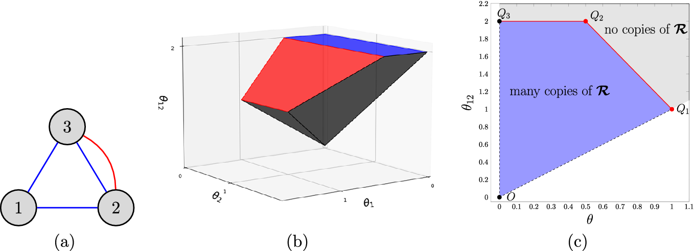
Example 2.3 Consider the edge-triangle multiplex as shown in Figure 2(a):

with
$E(\mathcal {R}^{(1)})= \{(1, 2), (2, 3), (1, 3)\}$
 , which corresponds to the triangle in layer 1 with edges colored in blue, and
$E(\mathcal {R}^{(2)}) = \{(2, 3)\}$
 , which corresponds to the edge in layer 2 colored in red. In this case, the main constraints determining the boundary of the region
$\partial _{\boldsymbol {\mathcal {R}}}^{+}$
 are:
-
• $2 \theta _1 + \theta _{12} < 3 $
: This corresponds to taking
$\boldsymbol F = \boldsymbol {\mathcal {R}}$
in (2.8). -
• $\theta _{12} < 2$
: This corresponds to taking
$\boldsymbol F = \boldsymbol {\mathcal {O}} := (\{2, 3\}, \mathcal {O}^{(1)}, \mathcal {O}^{(2)})$
, where
$\mathcal {O}^{(1)}$
and
$\mathcal {O}^{(2)}$
are both the single edge
$(2,3)$
.Figure 2(a) The edge-triangle multiplex $\boldsymbol {\mathcal {R}}$
defined in (2.9), (b) the full phase diagram in 3D, and (c) the 2D phase diagram assuming
$\theta _1=\theta _2= \theta $
.Figure 2 Long description
The figure consists of three panels labeled a, b, and c.
* Panel a is a network diagram with three nodes labeled 1, 2, and 3 arranged in a triangle. Blue straight lines connect all three nodes. A red curved line also connects nodes 2 and 3, representing a multiplex edge.
* Panel b is a three-dimensional plot with axes labeled theta sub 1, theta sub 2, and theta sub 1 2. It shows a complex geometric solid with red, blue, and dark gray faces representing a phase space volume.
* Panel c is a two-dimensional line graph. The x-axis is labeled theta and the y-axis is labeled theta sub 1 2. A blue-shaded polygonal region is bounded by points O at (0,0), Q sub 1 at (1,1), Q sub 2 at (0.5,2), and Q sub 3 at (0,2). The region inside the polygon is labeled many copies of R. The area outside the polygon, shaded in light gray, is labeled no copies of R. A solid red line connects Q sub 3 to Q sub 2 and Q sub 2 to Q sub 1. Dashed blue and black lines form the other boundaries of the blue region.


In addition one has the feasibility constraint
$\max \{\theta _1, \theta _2\} \leq \theta _{12}$
 . These together generate the three-dimensional satisfiability region shown in Figure 2(b): The red plane corresponds to the equation
$2 \theta _1 + \theta _{12} =3 $
 , the blue plane corresponds to
$\theta _{12} = 2$
 , and the black planes correspond to
$\max \{\theta _1, \theta _2\} = \theta _{12}$
 . In Figure 2(c), we show the two-dimensional slice of this region, where
$\theta _1=\theta _2= \theta $
 (this corresponds to the case where the graphs in the marginal layers have the same distribution). Then,
$\partial _{\boldsymbol {\mathcal {R}}}^+$
 is the two-dimensional region:

This is the blue polygonal region together with the blue line segment
$(O, Q_1)$
 (excluding the origin O and the point
$Q_1$
 ) shown in Figure 2(c). The threshold curve
$\partial _{\boldsymbol {\mathcal {R}}}$
 is the red polyline segment
$[Q_1, Q_2, Q_3)$
 (including the points
$Q_1$
 and
$Q_2$
 and excluding the point
$Q_3$
 ), and the unsatisfiability region
$\partial _{\boldsymbol {\mathcal {R}}}^{-}$
 is shown in gray in Figure 2(c). Note that for all points
$\boldsymbol \theta = (\theta , \theta _{12})$
 on the open segment
$(Q_1, Q_2)$
 ,
$\boldsymbol {\mathcal {R}}$
 is the unique
$\boldsymbol \theta $
 -extremal multiplex. On the other hand, for all points on the open segment
$(Q_2, Q_3)$
 , the multiplex
$\boldsymbol {\mathcal {O}}$
 defined above is the unique
$\boldsymbol \theta $
 -extremal multiplex. Also, at the point
$Q_2$
 , both
$\boldsymbol {\mathcal {R}}$
 and
$\boldsymbol {\mathcal {O}}$
 are
$\boldsymbol \theta $
 -extremal. Furthermore, at the point
$Q_1$
 , there are three
$\boldsymbol \theta $
 -extremal multiplexes: the original multiplex
$\boldsymbol {\mathcal {R}}$
 , the graph
$R^{(1)}$
 (which is the blue-colored triangle in layer 1), and the cross layer triangle on the vertices
$\{1,2, 3\}$
 formed by the blue edges
$\{(1, 2), (1, 3)\}$
 in layer 1 and the red edge
$(2, 3)$
 in layer 2.
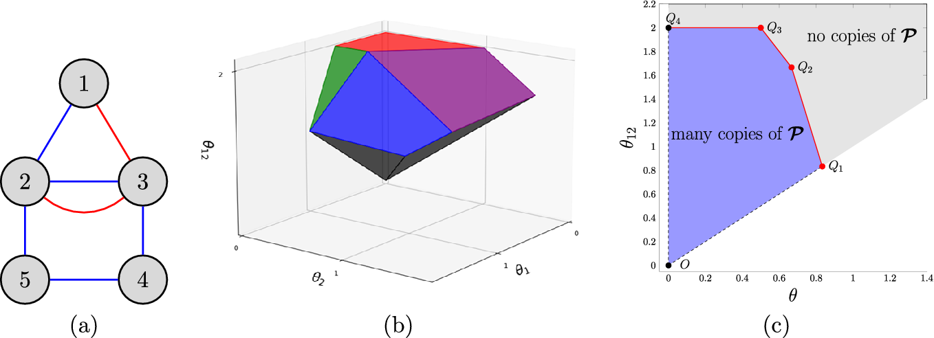
Example 2.4 Consider the multiplex shown in Figure 3(a):

where
$E(\mathcal {P}^{(1)}) = \{(1, 2), (2, 3), (2, 5), (3, 4), (4, 5)\}$
 , which is the graph in layer 1 with edges colored in blue, and
$E(\mathcal {P}^{(2)}) = \{(2, 3), (1, 3) \}$
 , which is the graph in layer 2 with edges colored in red.
(a) The multiplex
$\boldsymbol {\mathcal {P}}$
 defined in (2.10), (b) the full phase diagram in 3D, and (c) the 2D phase diagram assuming
$\theta _1=\theta _2= \theta $
 .

Figure 3 Long description
Panel a is a network graph with five numbered nodes. Node 1 is at the top, connected to nodes 2 and 3. Node 2 is connected to nodes 3 and 5. Node 3 is connected to node 4. Node 5 is connected to node 4. Edges are colored blue and red. Panel b is a 3D plot with axes theta sub 1, theta sub 2, and theta sub 1 2. It displays a complex 3D polytope with facets colored in green, red, blue, purple, and black. Panel c is a 2D graph with theta on the x-axis and theta sub 1 2 on the y-axis. A blue shaded region is bounded by points O at 0,0, Q sub 1, Q sub 2, Q sub 3, and Q sub 4. The blue region is labeled many copies of P. A gray shaded region to the right is labeled no copies of P. The boundary between the regions is marked with red line segments connecting the Q points.
The satisfiability region for this multiplex is shown in Figure 3(b), and the two-dimensional slice, where
$\theta _1=\theta _2= \theta $
 is shown in Figure 3(c). In this case, the satisfiability region
$\partial _{\boldsymbol {\mathcal {P}}}^+$
 is the blue polygonal region together with the blue line segment
$(O, Q_1)$
 (excluding the origin O and the point
$Q_1$
 ) as shown in Figure 3(c). The boundary curve
$\partial _{\boldsymbol {\mathcal {P}}}$
 is the red polyline segment
$[Q_1, Q_2, Q_3, Q_4)$
 (including the points
$Q_1$
 ,
$Q_2$
 , and
$Q_3$
 and excluding the point
$Q_4$
 ), and
$\partial _{\boldsymbol {\mathcal {P}}}^{-}$
 is the gray region in Figure 3(c). In this case, the
$\boldsymbol \theta $
 -extremal multiplexes on the boundary are:
-
• on the open line segment $(Q_1,Q_2)$
,
$\boldsymbol {\mathcal {P}}$
is uniquely
$\boldsymbol \theta $
-extremal; -
• on $(Q_2,Q_3)$
, the submultiplex induced on the vertices
$\{1, 2, 3\}$
is uniquely
$\boldsymbol \theta $
-extremal; -
• on $(Q_3,Q_4)$
, the submultiplex induced on the vertices
$\{2, 3\}$
(which is isomorphic to the multiplex
$\boldsymbol {\mathcal {O}}$
defined in Example 2.3) is uniquely
$\boldsymbol \theta $
-extremal.


Moreover, at the point
$Q_2$
 , both
$\boldsymbol {\mathcal {P}}$
 and the submultiplex induced on the vertices
$\{1, 2, 3\}$
 are
$\boldsymbol \theta $
 -extremal. Similarly, at
$Q_3$
 , both the submultiplexes induced on the vertices
$\{1, 2, 3\}$
 and
$\{2,3\}$
 are
$\boldsymbol \theta $
 -extremal. Furthermore, at
$Q_1$
 , there are three distinct
$\boldsymbol \theta $
 -extremal submultiplexes: the original multiplex
$\boldsymbol {\mathcal {P}}$
 and two non-induced submultiplexes
$\tilde {\boldsymbol {\mathcal {P}}}$
 and
$\boldsymbol {\mathcal {P}}'$
 defined as follows:
$\tilde {\boldsymbol {\mathcal {P}}} = \left (\{1,2,3,4,5\}, E(\mathcal {P}^{(1)}), \{(1,3)\}\right )$
 and
$\boldsymbol {\mathcal {P}}' = \left (\{1,2,3,4,5\}, E(\mathcal {P}^{(1)})\setminus \{(2,3)\}, E(\mathcal {P}^{(2)})\right )$
 .
Remark 2.5 (Boundedness of
$\partial _{\boldsymbol H}^+$
)

Note that the threshold for the existence of a single edge in the Erdős–Rényi model
$G(n, p_1)$
 is
$n^2 p_1 \gtrsim 1$
 . Hence, whenever the multiplex
$\boldsymbol H$
 has an edge that belongs to both the layers, one must have
$n^2p_{12} \gtrsim 1$
 for
$\boldsymbol H$
 to appear in
$G(n, p_1, p_2, p_{12})$
 . In the parametrization (2.5), this means
$\theta _{12} \leq 2$
 and, by the feasibility constraint,
$\max \{\theta _1, \theta _2\} \leq 2$
 . Hence, the satisfiability region
$\Delta _{\boldsymbol {H}}$
 will be a bounded polyhedral region whenever
$\boldsymbol {H}$
 has an edge that belongs to both layers.
2.2 Asymptotic normality in the satisfiability region
Once the threshold for the emergence of a multiplex
$\boldsymbol {H}$
 is obtained, the next natural question is to determine the limiting distribution of
$X(\boldsymbol {H}, \boldsymbol G_n)$
 in the satisfiability region (where
$\boldsymbol {G}_n$
 contains a diverging number of copies of
$\boldsymbol {H}$
 ). For the Erdős–Rényi random graph
$G(n, p_1)$
 , it is well known that the number of copies of a fixed subgraph H is asymptotically normal, whenever
$G_n$
 contains a diverging number of copies of H (which corresponds to the condition
$n p_1^{m_H} \gg 1$
 ) [Reference Barbour, Karoński and Ruciński3, Reference Janson17, Reference Nowicki26, Reference Ruciński33] (see [Reference Janson, Łuczak and Ruciński18, Chapter 6] for a comprehensive discussion). In this section, we will derive the analogous result for submultiplexes, under the parametrization (2.5).
To state the result, recall the definition of the Wasserstein distance between two random variables X and Z, to be denoted by
$d_{\mathrm {Wass}}(X, Z)$
 , from [Reference Chen, Goldstein and Shao11, Chapter 4]. Define

The following theorem establishes the asymptotic normality of
$Z(\boldsymbol H, \boldsymbol G_n)$
 with a rate of convergence in terms of the Wasserstein distance.
Theorem 2.6 Suppose
$\boldsymbol H = (V(\boldsymbol {H}), H^{(1)}, H^{(2)})$
 is a fixed multiplex with at least one edge. Then, with the parametrization (2.5), the following holds:

where
$\Delta _{\boldsymbol H}(\boldsymbol \theta )$
 is defined in (2.7). This implies that
$Z(\boldsymbol H, \boldsymbol G_n) \stackrel {D} \rightarrow N(0, 1)$
 , whenever
$\Delta _{\boldsymbol H}(\boldsymbol \theta )> 0$
 .
The proof of Theorem 2.6 is given in Section 4. The proof uses Stein’s method based on dependency graphs, which bounds the distance to normality in the Wasserstein distance. This result shows that the number of copies of any submultiplex
$\boldsymbol H$
 in the correlated Erdős–Rényi random multiplex
$\boldsymbol {G}_n$
 is asymptotically normal, for all parameter values for which the count of
$\boldsymbol H$
 in
$\boldsymbol G_n$
 diverges in probability, in the parametrization (2.5). This is depicted by the colored polyhedral regions in Figures 2 and 3 for their respective examples.
2.3 Distribution on the boundary surface
In this section, we consider the regime where
$\Phi _{\boldsymbol H} \asymp 1$
 (or in the parametrization (2.5),
$\Delta _{\boldsymbol H} = 0$
 ). This is the boundary between the regimes in which the probability of containing
$\boldsymbol H$
 in
$\boldsymbol {G}_n$
 tends to
$0$
 and
$1$
 , respectively. Deriving the distribution of
$X (\boldsymbol H, \boldsymbol G_n)$
 in this regime is an intriguing problem. To motivate our results, let us begin by recalling the analogous results for the Erdős–Rényi model
$G(n, p_1)$
 when
$p_1$
 is at the threshold (for a particular subgraph H). More precisely, consider a fixed subgraph H and
$G_n \sim G(n, p_1)$
 , such that
$n p_1^{m(H)} \rightarrow c \in (0, \infty )$
 satisfies the threshold condition (recall the definition of
$m(H)$
 from (2.4)). Then,
$X(H, G_n)$
 has the following properties:
-
(P1) If H is strictly balanced (recall Remark 2.2), then $X(H, G_n)$
converges to a Poisson distribution (see [Reference Janson, Łuczak and Ruciński18, Theorem 3.19]). -
(P2) If H is unbalanced, then $\mathbb {E}[X(H, G_n)] \gg 1$
at the threshold. In this case, there is a deterministic sequence
$a_n(H) \gg 1$
such that the asymptotic distribution of
$\frac {X(H, G_n)}{a_n(H) }$
coincides with that of
$X(H', G_n)$
, for a certain balanced subgraph
$H'$
of H. Hence, the problem reduces to the balanced case (see [Reference Ruciński34, Section 4] for details). -
(P3) If H is balanced, but not strictly balanced, then the limiting distribution of $X(H, G_n)$
can, in principle, be described (using the notion of grading [Reference Bollobás and Wierman8]), but it has no universal compact form. In particular, it depends on the structure and the number of subgraphs that maximize (2.4) (see [Reference Janson, Łuczak and Ruciński18, Section 3.3] for examples).


Our goal in this section is to derive analogous results for submultiplexes in the correlated Erdős–Rényi model. The first step toward this is to define the notion of balance in the multiplex setting. Note that since we have a threshold surface, the definition of balance will depend on which parameter value on the surface is chosen. For this, recall the definition of
$\ell _{\boldsymbol {F}}(\cdot )$
 from (2.8).
Definition 2.2 Fix a multiplex
$\boldsymbol H =(V(\boldsymbol H), H^{(1)}, H^{(2)})$
 and a point
$\boldsymbol \theta = (\theta _1, \theta _2, \theta _{12}) \in \partial _{\boldsymbol H}$
 . Then
$\boldsymbol H$
 is said to be
$\boldsymbol \theta $
 -balanced if
$\ell _{\boldsymbol H}(\boldsymbol \theta ) = 0$
 and

If the inequality in (2.13) is strict, then
$\boldsymbol H$
 is said to be strictly
$\boldsymbol \theta $
 -balanced. Furthermore, if
$\ell _{\boldsymbol H}(\boldsymbol \theta )> 0$
 and
$\ell _{\boldsymbol F}(\boldsymbol \theta ) = 0$
 , for some submultiplex
$\boldsymbol F \subset \boldsymbol H$
 , with
$|E(\boldsymbol F)| \geq 1$
 , then
$\boldsymbol H$
 is said to be
$\boldsymbol \theta $
 -unbalanced.
Remark 2.7 Note that
$\boldsymbol H$
 is
$\boldsymbol \theta $
 -balanced if and only if
$\boldsymbol H$
 is
$\boldsymbol \theta $
 -extremal (recall Definition 2.1).
We begin with the case when
$\boldsymbol {H}$
 is strictly
$\boldsymbol \theta $
 -balanced. Let
$\mathrm {Aut}(\boldsymbol H)$
 denote the collection of all permutations of
$V(\boldsymbol H)$
 that preserve the edge sets in both layers. Then we have the following result, which is proved in Section 5.
Theorem 2.8 Fix a multiplex
$\boldsymbol H =(V(\boldsymbol H), H^{(1)}, H^{(2)})$
 and a point
$\boldsymbol \theta = (\theta _1, \theta _2, \theta _{12}) \in \partial _{\boldsymbol H}$
 such that
$\boldsymbol {H}$
 is strictly
$\boldsymbol \theta $
 -balanced and
$\theta _{12}> \max \{\theta _1, \theta _2\}$
 . Then

Remark 2.9 The condition
$\theta _{12}>\max \{\theta _1,\theta _2\}$
 cannot, in general, be omitted if one wishes to obtain a Poisson limit. To see this, consider the multiplex
$\boldsymbol H = (\{1,2,3\}, H^{(1)}, H^{(2)} )$
 , where
$E(H^{(1)})=\left \{ (1,2) \right \}$
 and
$E(H^{(2)})=\left \{ (1,3) \right \}$
 . Thus,
$\boldsymbol H$
 consists of a two-edge path whose two edges belong to different layers. Suppose that
$\theta _1=\theta _2=\theta _{12}=\frac {3}{2}.$
 In this case,
$\boldsymbol H$
 is strictly
$\boldsymbol \theta $
 -balanced and the two layers of
$\boldsymbol G_n$
 coincide almost surely. Let
$Y_n$
 denote the number of copies of the two-edge path
$P_3$
 in the common graph
$G_n^{(1)}=G_n^{(2)} \sim G(n,n^{-\frac {3}{2}})$
 . Each copy of
$P_3$
 gives rise to exactly two distinct copies of
$\boldsymbol H$
 in
$\boldsymbol G_n$
 , corresponding to the two possible assignments of its two edges to the two layers. Therefore,
$X(\boldsymbol H,\boldsymbol G_n)=2Y_n$
 . Since
$P_3$
 is strictly balanced and
$\mathbb E[Y_n] \rightarrow \frac {1}{2}$
 , it follows from [Reference Janson, Łuczak and Ruciński18, Theorem 3.19] that
$Y_n\xrightarrow {D}\text {Pois}(\frac {1}{2})$
 . Hence,
$X(\boldsymbol H,\boldsymbol G_n) \stackrel {D} \rightarrow 2 \mathrm {Pois}(\frac {1}{2})$
 , which is a scaled Poisson distribution.
Next, we consider the case where
$\boldsymbol H$
 is
$\boldsymbol {\theta }$
 -unbalanced. In this case, we can rescale
$X(\boldsymbol {H}, \boldsymbol G_n)$
 such that its asymptotic distribution coincides with that of a
$\boldsymbol {\theta }$
 -balanced submultiplex of
$\boldsymbol {H}$
 . Toward this, we need a few definitions: To begin with, fix a point
$\boldsymbol \theta = (\theta _1, \theta _2, \theta _{12}) \in \partial _{\boldsymbol H}$
 and recall the notion of
$\boldsymbol \theta $
 -extremal from Definition 2.1. Denote the collection of
$\boldsymbol \theta $
 -extremal submultiplexes of
$\boldsymbol H$
 as
$\mathcal {A}_{\boldsymbol H}(\boldsymbol \theta )$
 . The core of
$\boldsymbol H$
 is defined as the largest
$\boldsymbol \theta $
 -extremal submultiplex of
$\boldsymbol H$
 , that is, the unique maximum element in
$\mathcal {A}_{\boldsymbol H}(\boldsymbol \theta )$
 in terms of multiplex containment (which is well defined by Lemma 6.1).Footnote
1
We also require the notion of an extension of a multiplex. Let
$\boldsymbol F\subseteq \boldsymbol H$
 be a fixed multiplex, and let
$\boldsymbol F'$
 be a copy of
$\boldsymbol F$
 . An extension of
$\boldsymbol F'$
 to
$\boldsymbol H$
 is a copy
$\boldsymbol H'$
 of
$\boldsymbol H$
 such that
$\boldsymbol F'\subseteq \boldsymbol H'$
 . Given a fixed copy
$\overline {\boldsymbol H}'$
 of the core
$\overline {\boldsymbol H}$
 , let
$\mathcal {E}_n(\overline {\boldsymbol H}';\overline {\boldsymbol H},\boldsymbol H)$
 denote the number of distinct copies
$\boldsymbol H'$
 of
$\boldsymbol H$
 satisfying
$\overline {\boldsymbol H}'\subseteq \boldsymbol H' \subseteq \boldsymbol G_n\cup \overline {\boldsymbol H}'$
 . By exchangeability, the distribution of this random variable does not depend on the particular copy
$\overline {\boldsymbol H}'$
 . We therefore write
$\mathcal {E}_n(\overline {\boldsymbol H},\boldsymbol H)$
 for a random variable having this common distribution.
Theorem 2.10 Fix a multiplex
$\boldsymbol H =(V(\boldsymbol H), H^{(1)}, H^{(2)})$
 and a point
$\boldsymbol \theta = (\theta _1, \theta _2, \theta _{12}) \in \partial _{\boldsymbol H}$
 . Then, with the parametrization (2.5),

The proof of Theorem 2.10 is given in Section 6. A main technical step in the proof is to show that the core
$\overline {\boldsymbol H}$
 is well defined. The challenge here is that, unlike in the case of graphs (single-layer networks), the notions of balanced/extremal depend on the parameter value
$\boldsymbol \theta \in \partial _{\boldsymbol H}$
 . The key observation here is that
$\ell _{\boldsymbol F}(\boldsymbol \theta )$
 is modular (see (6.2) for the definition), for
$\boldsymbol \theta \in \partial _{\boldsymbol H}$
 , as
$\boldsymbol F$
 ranges over the set of
$\boldsymbol \theta $
 -extremal multiplexes. Using this, we can establish that the core is well defined. Then by estimating the number of extensions of a planted core together with a second-moment argument, the result in (2.14) follows.
Remark 2.11 Note that Theorem 2.10 holds irrespective of whether
$\boldsymbol {H}$
 is
$\boldsymbol {\theta }$
 -balanced or
$\boldsymbol {\theta }$
 -unbalanced.
-
• When $\boldsymbol {H}$
is
$\boldsymbol {\theta }$
-balanced, then
$\overline {\boldsymbol {H}} = \boldsymbol {H}$
and
$\mathcal {E}_n(\overline {\boldsymbol {H}}', \boldsymbol {H}) = \mathcal {E}_n(\boldsymbol {H}', \boldsymbol {H}) = 1$
, for any copy
$\boldsymbol {H}'$
of
$\boldsymbol {H}$
. Hence, in this case, (2.14) holds trivially. -
• When $\boldsymbol {H}$
is
$\boldsymbol {\theta }$
-unbalanced, then
$\overline {\boldsymbol {H}} \subset \boldsymbol {H}$
and
$\mathbb {E}[X(\boldsymbol H, \boldsymbol G_n)] \gg 1$
. In this case, (2.14) shows that the asymptotic distribution of
$\frac {X(\boldsymbol H, \boldsymbol G_n)}{\mathbb {E}[\mathcal {E}_n(\overline {\boldsymbol {H}}, \boldsymbol {H})]}$
is the same as that of
$X(\overline {\boldsymbol H}, \boldsymbol G_n)$
. Since
$\boldsymbol \theta \in \partial _{\boldsymbol H}$
and
$\overline {\boldsymbol {H}}$
is
$\boldsymbol {\theta }$
-extremal, we also have
$\boldsymbol \theta \in \partial _{\overline {\boldsymbol H}}$
and
$\overline {\boldsymbol {H}}$
is
$\boldsymbol {\theta }$
-balanced. Hence, (2.14) reduces the problem to the balanced case.


A useful special case is when
$\boldsymbol H =(V(\boldsymbol H), H^{(1)}, H^{(2)})$
 is
$\boldsymbol {\theta }$
 -unbalanced such that
$|\mathcal A_{\boldsymbol H}(\boldsymbol \theta )| = 1$
 , that is, there is a unique
$\boldsymbol \theta $
 -extremal submultiplex (which is not
$\boldsymbol H$
 itself). Then the core
$\overline {\boldsymbol {H}}$
 is strictly
$\boldsymbol {\theta }$
 -balanced and invoking Theorems 2.8 and 2.10, we have the following result.
Corollary 2.12 Fix a multiplex
$\boldsymbol H =(V(\boldsymbol H), H^{(1)}, H^{(2)})$
 and a point
$\boldsymbol \theta = (\theta _1, \theta _2, \theta _{12}) \in \partial _{\boldsymbol H}$
 such that
$\theta _{12}> \max \{\theta _1, \theta _2\}$
 and
$|\mathcal A_{\boldsymbol H}(\boldsymbol \theta )| = 1$
 . Then,

To illustrate the above results, let us return to the edge-triangle multiplex from Example 2.3.
Example 2.13 (Example 2.3 continued)
Recall the edge-triangle multiplex
$\boldsymbol {\mathcal {R}}$
 from (2.9). Assume that
$\theta _1=\theta _2=\theta $
 . Note that
$|\mathrm {Aut}(\boldsymbol {\mathcal {R}})|=2$
 . In this case, the threshold curve
$\partial _{\boldsymbol {\mathcal {R}}}$
 is the red polyline segment
$[Q_1, Q_2, Q_3)$
 (including the point
$Q_1$
 and excluding the point
$Q_3$
 ) as shown in Figure 2(c). Depending on the location of the point
$\boldsymbol \theta = (\theta , \theta _{12})$
 on this polyline segment, we have the following cases:
-
• $\boldsymbol \theta $
lies on the open segment
$(Q_1, Q_2)$
. Here,
$\boldsymbol {\mathcal {R}}$
is the unique
$\boldsymbol \theta $
-extremal multiplex. Hence, on this line segment,
$\boldsymbol {\mathcal {R}}$
is strictly
$\boldsymbol \theta $
-balanced and Theorem 2.8 implies $$ \begin{align*}X(\boldsymbol{\mathcal{R}}, \boldsymbol G_n) \stackrel{D} \rightarrow \mathrm{Pois}(\tfrac{1}{2}).\end{align*} $$
-
• $\boldsymbol \theta $
lies on the open segment
$(Q_2, Q_3) = \{(\theta , 2) : 0 < \theta < \tfrac {1}{2} \}$
. Here, the multiplex
$\boldsymbol {\mathcal {O}}$
defined in Example 2.3 is the unique
$\boldsymbol \theta $
-extremal submultiplex. Hence, on this line segment,
$\boldsymbol {\mathcal {R}}$
is
$\boldsymbol \theta $
-unbalanced with
$|\mathcal A_{\boldsymbol {\mathcal {R}}}(\boldsymbol \theta )| = 1$
, which means Corollary 2.12 can be applied. For this, we need to compute
$\mathbb {E}[\mathcal {E}_n(\overline {\boldsymbol {\mathcal {R}}}, \boldsymbol {\mathcal {R}})]$
. To this end, without loss of generality, assume that a copy of the multiplex
$\boldsymbol {\mathcal {O}}$
is planted on the vertices
$\{1, 2\}$
of
$\boldsymbol G_n$
. To extend this copy of
$\boldsymbol {\mathcal {O}}$
to a copy of
$\boldsymbol {\mathcal {R}}$
, we need to choose another vertex
$v \in [n]\backslash \{1, 2\}$
(for which we have
$(n-2)$
choices) and ensure that the edges
$(1, v)$
and
$(2, v)$
are present in the first layer of
$\boldsymbol {G}_n$
(which has probability
$p_{1}^2 = n^{-2\theta }$
). Hence,
$\mathbb {E}[\mathcal {E}_n(\overline {\boldsymbol {\mathcal {R}}}, \boldsymbol {\mathcal {R}})] \sim n^{1-2 \theta }$
. Hence, applying Corollary 2.12 gives $$ \begin{align*} \frac{X(\boldsymbol{\mathcal{R}}, \boldsymbol G_n)}{n^{1-2 \theta}} \xrightarrow{D} \mathrm{Pois}\left(\tfrac{1}{ 2 }\right). \end{align*} $$
-
• Next, suppose $\boldsymbol \theta = Q_2 = (\frac {1}{2}, 2)$
. In this case, both
$\boldsymbol {\mathcal {R}}$
and
$\boldsymbol {\mathcal {O}}$
are
$\boldsymbol \theta $
-extremal. This means at this point
$\boldsymbol {\mathcal {R}}$
is
$\boldsymbol \theta $
-balanced, but not strictly
$\boldsymbol \theta $
-balanced. This setting is not covered by the general results discussed above. In fact, in this case, the asymptotic distribution of
$X(\boldsymbol {\mathcal {R}}, \boldsymbol G_n)$
is not Poisson. By a direct calculation, it can be shown that $$ \begin{align*} X(\boldsymbol{\mathcal{R}}, \boldsymbol G_n) \xrightarrow{D} \sum_{i=1}^Z Z_i , \end{align*} $$where $Z \sim \mathrm {Pois}(\frac {1}{2})$
and independently
$Z_1, Z_2, \ldots $
are i.i.d.
$\mathrm {Pois}(1)$
random variables. The idea behind this is as follows: Note that
$\theta _{12} = 2$
implies
$p_{12} = \frac {1}{n^2}$
. This means the asymptotic distribution of
$X(\boldsymbol {\mathcal {O}}, \boldsymbol {G}_n)$
is
$\mathrm {Pois}(\frac {1}{2})$
. Moreover, each copy of the multiplex
$\boldsymbol {\mathcal {O}}$
in
$\boldsymbol {G}_n$
has asymptotically
$\mathrm {Pois}(1)$
number of common neighbors in layer 1 of
$\boldsymbol G_n$
(since
$\theta = \frac {1}{2}$
means
$p_1 = \frac {1}{\sqrt n}$
), each of which forms a copy of
$\boldsymbol {\mathcal {R}}$
in
$\boldsymbol {G}_n$
.
-
• The remaining case is $\boldsymbol \theta = Q_1 = (1, 1)$
. In this case, recall from Example 2.3 that there are three
$\boldsymbol \theta $
-extremal submultiplexes (one of which is
$\boldsymbol {\mathcal {R}}$
itself). This means, at this point,
$\boldsymbol {\mathcal {R}}$
is
$\boldsymbol \theta $
-balanced, but not strictly
$\boldsymbol \theta $
-balanced, as in the previous case. Note that this corresponds to the parameter values
$p_1=p_2= p_{12} = \frac {1}{n}$
, that is, the layers of
$\boldsymbol G_n$
are perfectly correlated. Hence, given a triangle in layer 1 of
$\boldsymbol G_n$
, there are three ways to choose the red edge in layer 2 of
$\boldsymbol G_n$
(refer to Figure 2(a)) to obtain a copy of
$\boldsymbol {\mathcal {R}}$
in
$\boldsymbol G_n$
. This implies $$ \begin{align*}X(\boldsymbol{\mathcal{R}}, G_n) = 3 X(R^{(1)}, G_n^{(1)}) \stackrel{D} \rightarrow 3 \mathrm{Pois}(\tfrac{1}{6}) ,\end{align*} $$since the number of triangles in $G(n, p_1)$
when
$np_1 \rightarrow 1$
, converges to
$\mathrm {Pois}(\frac {1}{6})$
(see [Reference Janson17, Theorem 3.19]).


3 Proof of Theorem 2.1
Let
$\boldsymbol G_n = ([n], G_n^{(1)}, G_n^{(2)}) \sim G(n, p_1, p_2, p_{12})$
 be a sample from the correlated Erdős–Rényi model as in Definition 1.1. Fix a multiplex
$\boldsymbol H = (V(\boldsymbol {H}), H^{(1)}, H^{(2)})$
 with at least one edge. Recalling (2.1), note that if
$\mathcal {H}_n=\{\boldsymbol H_1,\,\boldsymbol H_2,\,\ldots ,\, \boldsymbol H_M\}$
 is the collection of all copies of
$\boldsymbol H$
 in the complete multiplex
$\boldsymbol {K}_n$
 with vertex set
$[n]$
 , where
$M = X(\boldsymbol {H}, \boldsymbol {K}_n)$
 , then

With this representation, in the following lemma, we compute the asymptotic orders of the mean and the variance of
$X(\boldsymbol {H}, \boldsymbol {G}_n)$
 . For this, it is convenient to define, for a multiplex
$\boldsymbol H = (V(\boldsymbol H), H^{(1)}, H^{(2)})$
 ,

Lemma 3.1 For any multiplex
$\boldsymbol H = (V(\boldsymbol {H}), H^{(1)}, H^{(2)})$
 with at least one edge,

Furthermore,

Further, under the parametrization (2.5), one has the following:

Proof From (3.1), we have

since
$X(\boldsymbol {H}, \boldsymbol {K}_n) \asymp _{\boldsymbol H} n^{|V(\boldsymbol H)|}$
 .
Next, we compute
$\mathrm {Var} \left [X(\boldsymbol {H}, \boldsymbol {G}_n) \right ]$
 . From (3.1),

For
$\boldsymbol H_s, \boldsymbol H_t \in \mathcal H_n$
 , assume
$\boldsymbol {H}_s=(V(\boldsymbol H_s), H_s^{(1)},H_s^{(2)})$
 and
$\boldsymbol {H}_t=(V(\boldsymbol H_t), H_t^{(1)},H_t^{(2)})$
 . Let
$\boldsymbol {J}=\boldsymbol {H}_s\cup \boldsymbol {H}_t$
 . Then,

Now, for notational convenience, let
$A_s:=E(H_s^{(1)})$
 ,
$B_s:=E(H_s^{(2)})$
 ,
$A_t:=E(H_t^{(1)})$
 , and
$B_t:=E(H_t^{(2)})$
 . Then the (one-sided) overlap multiplex
$\boldsymbol F_{s, t}= (V(\boldsymbol F_{s, t}), F_{s, t}^{(1)},F_{s, t}^{(2)})$
 is defined as follows:
$V(\boldsymbol F_{s, t}):=V(\boldsymbol H_s)\cap V(\boldsymbol H_t)$
 , and
$ E(F_{s, t}^{(1)}) := A_s\cap (A_t\cup B_t) \text { and } E(F_{s, t}^{(2)}) := B_s\cap (A_t\cup B_t)$
 . Thus,
$\boldsymbol F_{s, t}$
 retains every underlying edge of
$\boldsymbol H_s$
 that is also used by
$\boldsymbol H_t$
 , while preserving its original layer type in
$\boldsymbol H_s$
 . In particular,
$\boldsymbol F_{s, t} \subseteq \boldsymbol H_s$
 , and, hence, it is isomorphic to a submultiplex of
$\boldsymbol H$
 . (Note that, since
$\boldsymbol F_{s, t}$
 is one-sided,
$\boldsymbol F_{s, t} \ne \boldsymbol F_{t, s} $
 , in general, although the following argument would work with
$F_{t, s} $
 as well.) We now claim that

To prove this, define
$D_{s,t}^{(1)}:=B_s\cap (A_t\setminus B_t)$
 and
$D_{s,t}^{(2)}:=A_s\cap (B_t\setminus A_t)$
 . Then, a set-theoretic calculation gives

where the last step uses
$p_{12} \leq \min \{p_1, p_2\}$
 . Combining the above proves (3.8).
Furthermore,
$\mathbb P\left (\boldsymbol H_s\subseteq \boldsymbol G_n\right )^2= \lambda _{p_1,p_2,p_{12}}(\boldsymbol H)^2$
 . Therefore,

For every fixed submultiplex
$\boldsymbol F\subseteq \boldsymbol H$
 , the number of ordered pairs
$(\boldsymbol H_s,\boldsymbol H_t)$
 such that
$\boldsymbol F_{s, t}\cong \boldsymbol F$
 is at most
$\lesssim _{\boldsymbol H} n^{2|V(\boldsymbol H)|-|V(\boldsymbol F)|}$
 . Combining this with (3.6) and (3.9), the result in (3.3) follows.
To prove (3.4), we have to show the corresponding lower bound also holds, under the parametrization (2.5). To begin with, for
$U \subset V(\boldsymbol H)$
 , denote by
$\boldsymbol H[U]$
 the submultiplex of
$\boldsymbol H$
 induced on the set of vertices U. Then

Further, using
$p_{12}\leq \min \{p_1,p_2\}\leq 1$
 gives
$ n^{|V(\boldsymbol F)|}\lambda _{p_1, p_2, p_{12}}(\boldsymbol F) \geq $
 $ n^{|V(\boldsymbol F)|} \lambda _{p_1, p_2, p_{12}} (\boldsymbol H[V(\boldsymbol F)])$
 . Since
$\boldsymbol H$
 is fixed, there are only
$\lesssim _{\boldsymbol H} 1$
 submultiplexes with a prescribed vertex set. Hence,

Now, fix
$U\subseteq V(\boldsymbol H)$
 and denote by
$\tilde {\mathcal P}_U$
 , the collection of ordered pairs of injective maps
$\varphi _s,\varphi _t:V(\boldsymbol H)\longrightarrow [n]$
 , satisfying
$\varphi _s|_U=\varphi _t|_U$
 and
$\varphi _s(V(\boldsymbol H))\cap \varphi _t(V(\boldsymbol H)) =\varphi _s(U)=\varphi _t(U)$
 . Define
$\mathcal P_U$
 to be the collection of ordered pairs of copies
$\left (\boldsymbol H_{\varphi _s},\boldsymbol H_{\varphi _t}\right )$
 arising from pairs
$(\varphi _s, \varphi _t)\in \tilde {\mathcal P}_U$
 . Note that for every
$(\boldsymbol H_s, \boldsymbol H_t) \in \mathcal P_U$
 , the common edges of
$\boldsymbol H_s$
 and
$\boldsymbol H_t$
 are precisely the edges of
$\boldsymbol H[U]$
 , with the same layer types in the two copies. Consequently,

Since
$\boldsymbol H[U]$
 contains an edge, under the scaling (2.5), it follows that
$\lambda _{p_1, p_2, p_{12}} (\boldsymbol H[U]) \ll 1$
 . Combining this with the bound
$|\mathcal P_U| \asymp _{\boldsymbol H} n^{2 |V(\boldsymbol H)|-|U|}$
 gives

Note that a fixed ordered pair of copies can belong to
$\mathcal P_U$
 for at most
$\lesssim _{\boldsymbol H} 1$
 choices of U. Consequently, after dividing by this bounded multiplicity, if necessary, the LHS of (3.11) is bounded above by a constant multiple of the sum of the positive covariance terms in the variance expansion. Further, the contribution from the negative covariance terms is negligible relative to (3.11) under (2.5). Hence, from (3.10) and (3.11), the required lower bound in (3.4) follows.
With the above lemma, we can complete the proof of Theorem 2.1. First, suppose
$\Phi _{\boldsymbol H} \ll 1$
 . Let
$\boldsymbol {F}$
 be a submultiplex where the minimum for
$\Phi _{\boldsymbol H}$
 is attained (recall (2.3)). Then, from (3.2),

This proves the 0-statement in Theorem 2.1.
Next, suppose
$\Phi _{\boldsymbol {H}} \gg 1$
 . Then, by Lemma 3.1,

This means,
$\frac {X(\boldsymbol H, \boldsymbol G_n)}{\mathbb {E}[X(\boldsymbol H, \boldsymbol G_n)]} \stackrel {P} \rightarrow 1$
 , which implies
$X(\boldsymbol {H}, \boldsymbol {G}_n) \stackrel {P} \rightarrow \infty $
 , since
${\mathbb {E}[X(\boldsymbol H,G_n)] \kern1.3pt{\rightarrow}\kern1.3pt \infty }$
 , whenever
$\Phi _{\boldsymbol H} \gg 1$
 . This completes the proof of Theorem 2.1.
4 Proof of Theorem 2.6
The proof of Theorem 2.6 will use Stein’s method based on dependency graphs. We begin by defining the notion of a dependency graph.
Definition 4.1 (Dependency graph)
Let
$\{X_v\}_{v\in V}$
 be a family of random variables (defined on some common probability space) indexed by a finite set V. Then a graph
$\mathcal G$
 with vertex set V is said to be a dependency graph for the collection
$\{X_v\}$
 if the following holds: For any two subsets of vertices
$A, B \subseteq V$
 such that there is no edge in
$\mathcal {G}$
 from any vertex in A to any vertex in B, the collections of random variables
$\{X_v\}_{v\in A}$
 and
$\{X_v\}_{v\in B}$
 are independent.
For a dependency graph
$\mathcal G$
 and
$u \in V$
 , denote by
$\overline {N}_{\mathcal {G}}(u)$
 , the set of neighbors of u in
$\mathcal {G}$
 and u itself. Also, denote
$\overline {N}_{\mathcal {G}}(u,\,v):=\overline {N}_{\mathcal {G}}(u)\cup \overline {N}_{\mathcal {G}}(v).$
 We will use the following version of Stein’s method based on dependency graph.
Theorem 4.1 [Reference Janson, Łuczak and Ruciński18, Theorem 6.33]
Suppose
$\{X_v\}_{v\in V}$
 be a family of random variables with dependency graph
$\mathcal {G}$
 . Assume
$\mathbb {E}[X_v]=0$
 , for all
$v\in V.$
 Let
$W=\frac {1}{\sigma }\sum _{v\in V}X_v$
 , where
$\sigma ^2=\mathrm {Var}[\sum _{v\in V}X_v]$
 . Assume, for all
$u,\,v\in V,$
 the following bounds hold:

Then, for
$Z \sim N(0, 1)$
 ,
$d_{\mathrm {Wass}}(W, Z)\lesssim \frac {RQ^2}{\sigma ^3}$
 .
With the above preparations, we can now proceed with the proof of Theorem 2.6. As before, let
$\mathcal {H}_n=\{\boldsymbol H_1,\,\boldsymbol H_2,\,\ldots ,\, \boldsymbol H_M\}$
 be the collection of all copies of
$\boldsymbol H$
 in
$\boldsymbol {K}_n$
 , where
$M = X(\boldsymbol {H}, \boldsymbol {K}_n)$
 . For
$1\le s \le M$
 , define
$I_s:=\boldsymbol {1}\{ \boldsymbol H_s \subseteq \boldsymbol G_n\}$
 and

where
$\mu = \lambda _{p_1, p_2, p_{12}}(\boldsymbol H)$
 (recall (3.5)). Define
$\sigma ^2= \mathrm {Var}[X(\boldsymbol H,\, \boldsymbol G_n)]$
 . Recalling (2.12), note that
$Z(\boldsymbol H, \boldsymbol G_n) = \frac {1}{\sigma } \sum _{s=1}^{M}X_s$
 . Construct a dependency graph
$\mathcal G$
 of the collection of random variables
$\{X_s : \boldsymbol H_s \in \mathcal {H}_n\}$
 on the vertex set
$\{1,\,2,\,\ldots ,\,M\}$
 as follows: Connect the edge
$(s,\,t)$
 , for
$1 \leq s < t \leq M$
 in
$\mathcal {G}$
 whenever
$|E(\boldsymbol H_s)\cap E(\boldsymbol H_t)| \geq 1$
 . (Recall that for any multiplex
$\boldsymbol H = (V(\boldsymbol H), H^{(1)}, H^{(2)})$
 ,
$E(\boldsymbol H):=E(H^{(1)})\cup E(H^{(2)}$
 .)
To apply Theorem 4.1, first note that
$\mathbb {E}|X_s| = 2\mu (1-\mu ) \leq 2 \mu $
 . Hence,
$R_n := \sum _{s=1}^M\mathbb {E}|X_s| \lesssim _{\boldsymbol H} M\mu = \mathbb {E}[X(\boldsymbol H,\boldsymbol G_n)],$
 where the last step follows from (3.5). Next, fix
$s, t \in \{1, 2, \ldots , M\}$
 . For
$w\in \overline N_{\mathcal G}(s,t)$
 , define the (one-sided) overlap multiplex
$\boldsymbol H_{w, \{s,t\} }= (V(\boldsymbol H_{w, \{s,t\} }), H_{w, \{s,t\} }^{(1)}, H_{w, \{s,t\} }^{(2)} )$
 as:
$V(\boldsymbol H_{w, \{s,t\} }):= V(\boldsymbol H_w)\cap (V(\boldsymbol H_s)\cup V(\boldsymbol H_t) )$
 and
$E(H_{w, \{s,t\} }^{(1)})\ {:=}\ E(H_w^{(1)})\ {\cap}\ ( E(\boldsymbol H_s)\ {\cup}\ E(\boldsymbol H_t) )$
 and
$E(H_{w, \{s,t\} }^{(2)})\ {:=} E(H_w^{(2)})\cap ( E(\boldsymbol H_s)\cup E(\boldsymbol H_t) )$
 . Note that
$\boldsymbol H_{w, \{s,t\} }\subseteq \boldsymbol H_w$
 . Further, since
$w\in \overline N_{\mathcal G}(s,t)$
 ,
$|E(\boldsymbol H_{w, \{s,t\} })|\geq 1$
 . Let
$\mathcal A_{w, \{s,t\}}$
 denote the event that all edge requirements of
$\boldsymbol H_w$
 whose underlying vertex pairs lie outside
$E(\boldsymbol H_s)\cup E(\boldsymbol H_t)$
 are satisfied. Then
$\{\boldsymbol H_w\subseteq \boldsymbol G_n\} \subseteq \mathcal A_{w, \{s,t\}}$
 . Note that the event
$\mathcal A_{w, \{s,t\}}$
 depends only on the edge vectors outside
$E(\boldsymbol H_s)\cup E(\boldsymbol H_t)$
 . Hence,

Then recalling that
$\mu = \lambda _{p_1, p_2, p_{12}}(\boldsymbol H)$
 ,
$X_w = I_w - \mu $
 , and using
$|X_w| \leq I_w + \mu $
 ,

For every fixed submultiplex
$\boldsymbol F\subseteq \boldsymbol H$
 , the number of copies
$\boldsymbol H_w$
 satisfying
$\boldsymbol H_{w, \{s,t\} }\cong \boldsymbol F$
 is
$\lesssim _{\boldsymbol H} n^{|V(\boldsymbol H)|-|V(\boldsymbol F)|}$
 . Therefore, uniformly in
$s,t$
 ,

where the last step uses (3.5). Now, recall from (3.4) that
$ \sigma ^2 = \mathrm {Var} [ X( \boldsymbol {H}, \boldsymbol G_n)] \asymp _{\boldsymbol H} \frac { (\mathbb {E} [X(\boldsymbol H, \boldsymbol G_n)])^2}{ \Phi _{\boldsymbol {H}}}$
 , under the parametrization (2.5). Combining the above with Theorem 4.1 gives the result in (2.12), as required.
5 Proof of Theorem 2.8
We will prove Theorem 2.8 using the Stein–Chen method for Poisson approximation based on dependency graphs.
Theorem 5.1 [Reference Chatterjee, Diaconis and Meckes10, Theorem 15]
Suppose
$\{X_\alpha :\alpha \in A\}$
 be collection of Bernoulli random variables and
$X:=\sum _{\alpha \in A} X_\alpha $
 . Let
$\mathcal G$
 be a dependency graph for this collection. Then, with
$\lambda :=\mathbb E[X]$
 , the following holds:

where

(Here,
$d_{\mathrm {TV}}$
 denotes the total variation distance between two random variables.)
As in the proof of Theorem 2.6, define
$I_s:=\boldsymbol {1}\{ \boldsymbol H_s \subseteq \boldsymbol G_n\}$
 , for
$1 \leq s \leq M$
 . Recall, from (3.5), that
$\mu := \mathbb E[I_s] = \lambda _{p_1,p_2,p_{12}}(\boldsymbol H)= n^{- |V(\boldsymbol H)|}, $
 where the last equality uses
$\ell _{\boldsymbol H}(\boldsymbol \theta )=0$
 , since
$\boldsymbol H$
 is
$\boldsymbol \theta $
 -balanced. This implies that
$\lambda := \mathbb E[X(\boldsymbol H,\boldsymbol G_n)] \rightarrow \frac {1}{|\mathrm {Aut}(\boldsymbol H)|}$
 . Construct a dependency graph
$\mathcal G$
 of the collection of random variables
$\{I_s : 1 \leq s \leq M \}$
 , as in the proof of Theorem 2.6.
To apply Theorem 5.1, first note that, for any
$1 \leq s \leq M$
 , one has
$|\overline {N}_{\mathcal {G}}(s)| \lesssim _{\boldsymbol H} n^{|V(\boldsymbol H)|-2}$
 . Then, since
$M \asymp _{\boldsymbol H} n^{|V(\boldsymbol H)|}$
 ,

It remains to estimate
$B_2$
 . For this, fix two distinct adjacent copies
$\boldsymbol H_s$
 and
$\boldsymbol H_t$
 in the dependency graph and denote by
$F_{\{s, t\}}$
 the (one-sided) overlap multiplex as defined in the proof of Lemma 3.1. Then from (3.8),

We now consider the following two cases.
Case
$1$
 :
$\boldsymbol F_{\{s, t\}}$
 is a proper submultiplex of
$\boldsymbol H$
 . In this case, the number of ordered pairs
$(s, t)$
 satisfying
$\boldsymbol F_{\{s, t\}}\cong \boldsymbol F$
 is at most
$\lesssim _{\boldsymbol H} n^{2 |V(\boldsymbol H)|-|V(\boldsymbol F)|}$
 . Therefore, using (5.2), the total contribution to
$B_2$
 of all such pairs is at most

where the last step follows by noting that
$\ell _{\boldsymbol F}(\boldsymbol \theta )>0$
 for every proper submultiplex
$\boldsymbol F\subsetneq \boldsymbol H$
 containing an edge, since
$\boldsymbol H$
 is strictly
$\boldsymbol \theta $
 -balanced.
Case
$2$
 :
$\boldsymbol F_{\{s, t\}}\cong \boldsymbol H$
 . In this case, the two copies have the same vertex set and the same underlying edge support, but since
$s\neq t$
 , their layer assignments cannot be identical. This means that relative to one of the two copies, the joint occurrence requires an additional layer on at least one underlying edge. Consequently, for at least one underlying edge, the joint occurrence of the two copies incurs an additional factor of either
$p_{12}/p_1$
 or
$p_{12}/p_2$
 relative to the occurrence probability of one copy. This implies,
$\mathbb P(I_s=I_t=1) \leq \mu n^{-\eta }$
 , where
$\eta = \min \left \{ \theta _{12}-\theta _1,\, \theta _{12}-\theta _2 \right \}>0$
 , by assumption. Moreover, for each
$1\leq s\leq M$
 , there are only
$\lesssim _{\boldsymbol H} 1 $
 choices of t, having the same vertex set and underlying edge support as
$\boldsymbol H_s$
 . Therefore, the total contribution to
$B_2$
 in this case is at most

Combining (5.1), (5.3), and (5.4) with Theorem 5.1, the result in Theorem 2.8 follows.
6 Proof of Theorem 2.10
Fix a point
$\boldsymbol \theta = (\theta _1, \theta _2, \theta _{12}) \in \partial _{\boldsymbol H}$
 . Recall that,
$\mathcal {A}_{\boldsymbol H}(\boldsymbol \theta )$
 denotes the collection of
$\boldsymbol \theta $
 -extremal submultiplexes of
$\boldsymbol H$
 . We begin by showing that the core
$\overline {\boldsymbol {H}}$
 of
$\boldsymbol {H}$
 , which is the maximal element of
$\mathcal {A}_{\boldsymbol H}(\boldsymbol \theta )$
 under containment, is well defined. Toward this, we need the notion of completion of a multiplex. Throughout, whenever we consider a submultiplex
$\boldsymbol F$
 of
$\boldsymbol H$
 , we will implicitly assume that
$|E(\boldsymbol F)| \geq 1$
 .
Definition 6.1 Let
$\boldsymbol F \subseteq \boldsymbol H$
 be a submultiplex. Define the completion
$\hat {\boldsymbol F} = (V(\boldsymbol F), \hat {F}^{(1)}, \hat {F}^{(2)}), $
 of
$\boldsymbol F = (V(\boldsymbol F), F^{(1)}, F^{(2)})$
 as the multiplex withFootnote
2

for
$i \in \{1, 2\}$
 . If
$\boldsymbol F=\hat {\boldsymbol F}$
 , then we call the submultiplex complete.
With this definition, we can show that the core of
$\boldsymbol H$
 is well defined.
Lemma 6.1 If
$ \boldsymbol {Q}, \boldsymbol {R} \in \mathcal {A}_{\boldsymbol H}(\boldsymbol \theta )$
 , then
$\hat { \boldsymbol {Q}}\cup \hat { \boldsymbol {R}} \in \mathcal {A}_{\boldsymbol H}(\boldsymbol \theta )$
 . Consequently, the maximum element in
$\mathcal {A}_{\boldsymbol H}(\boldsymbol \theta )$
 and the core
$\overline {\boldsymbol H}$
 is well defined.
Proof We begin with the following fact (which is proved later in Section 6.1):

Hence, without loss of generality, we may assume that
$ \boldsymbol {Q} = \hat { \boldsymbol {Q}}$
 and
$ \boldsymbol {R} = \hat { \boldsymbol {R}}$
 . Now, recall the definition of the function
$\ell _{\boldsymbol F}(\boldsymbol \theta )$
 from (2.8). The key observation is that the function
$\ell _{\boldsymbol F}(\boldsymbol \theta )$
 is modular, that is,

for
$ \boldsymbol {Q}, \boldsymbol {R} \in \mathcal {A}_{\boldsymbol H}(\boldsymbol \theta ) $
 which are both complete. We prove this fact in Section 6.2 below. This implies, since
$\ell _{\boldsymbol {Q}}(\boldsymbol {\theta }) = \ell _{\boldsymbol {R}}(\boldsymbol {\theta }) = 0$
 (recall
$\boldsymbol {Q}\ and\ \boldsymbol {R}$
 are
$\boldsymbol \theta $
 -extremal),

Also, since
$\boldsymbol \theta \in \partial _{\boldsymbol H}$
 , we have
$\ell _{\boldsymbol {F}}(\boldsymbol {\theta }) \geq 0$
 for all submultiplexes
$\boldsymbol F \subseteq \boldsymbol H$
 . This means,
$\ell _{\boldsymbol {Q}\cap \boldsymbol {R}}(\boldsymbol {\theta }) \geq 0$
 and
$\ell _{\boldsymbol {Q}\cup \boldsymbol {R}}(\boldsymbol {\theta }) \geq 0$
 , since
$\boldsymbol {Q}\ and\ \boldsymbol {R}$
 are both submultiplexes of
$\boldsymbol {H}$
 . Hence, (6.3) can hold only if
$\ell _{\boldsymbol {Q}\cup \boldsymbol {R}}(\boldsymbol {\theta }) = 0$
 , which means
$\boldsymbol {Q}\cup \boldsymbol {R}$
 is a
$\boldsymbol \theta $
 -extremal submultiplex of
$\boldsymbol H$
 .
6.1 Proof of (6.1)
We begin with the following lemma.
Lemma 6.2 Fix a multiplex
$\boldsymbol F_1 = (V(\boldsymbol F_1), F_1^{(1)}, F_1^{(2)})$
 . Define
$\boldsymbol F_2=\boldsymbol F_1\cup \boldsymbol {\mathcal {O}}_{(u, v)}$
 , where
$\boldsymbol {\mathcal {O}}_{(u, v)}$
 is a multiplex with vertex set
$\{u, v\} \subseteq V(\boldsymbol F_1)$
 with the edge
$(u, v) $
 present in both layers. Then
$\ell _{\boldsymbol F_1}(\boldsymbol \theta )\geq \ell _{\boldsymbol F_2}(\boldsymbol \theta )$
 , for
$\boldsymbol \theta \in \Theta $
 .
Proof If
$(u,v) \in E(F_1^{(1)}) \cap E(F_1^{(2)})$
 , then
$\boldsymbol F_1=\boldsymbol F_2$
 and
$\ell _{\boldsymbol F_1}(\boldsymbol \theta )= \ell _{\boldsymbol F_2}(\boldsymbol \theta )$
 . Otherwise, there are the following three possibilities:
-
(1) $(u,v)\notin E(F_1^{(1)})\cup E(F_1^{(2)})$
: Then, as
$\theta _{12}> 0 $
, $$ \begin{align*} \ell_{\boldsymbol F_2}(\boldsymbol \theta) =|V(\boldsymbol{F_1})| &- \theta_1 |E(F_1^{(1)})\setminus E(F_1^{(2)})| - \theta_2 |E(F_1^{(2)})\setminus E(F_1^{(1)})| \\ & - \theta_{12} (|E(F_1^{(1)})\cap E(F_1^{(2)})|+1) < \ell_{\boldsymbol{F_1}}(\boldsymbol \theta). \end{align*} $$
-
(2) $(u,v)\in E(F_1^{(1)})\setminus E(F_1^{(2)})$
: Then, as
$\theta _{12}\geq \theta _1$
, $$ \begin{align*} \ell_{\boldsymbol F_2}(\boldsymbol \theta) =|V(\boldsymbol{F_1})| &- \theta_1 (|E(F_1^{(1)}) \setminus E(F_1^{(2)})| -1) - \theta_2 |E(F_1^{(2)})\setminus E(F_1^{(1)})| \\ & - \theta_{12} (|E(F_1^{(1)})\cap E(F_1^{(2)})|+1) \leq\ell_{\boldsymbol F_1}(\boldsymbol \theta). \end{align*} $$
-
(3) $(u,v)\in E(F_1^{(2)})\setminus E(F_1^{(1)})$
: Then, as
$\theta _{12}\geq \theta _2$
, $$ \begin{align*} \ell_{\boldsymbol F_2}(\boldsymbol \theta) = |V(\boldsymbol{F_1})| &- \theta_1 |E(F_1^{(1)})\setminus E(F_1^{(2)})| - \theta_2 (|E(F_1^{(2)})\setminus E(F_1^{(1)})|-1) \\ & - \theta_{12} (|E(F_1^{(1)})\cap E(F_1^{(2)})|+1) \leq \ell_{\boldsymbol F_1}(\boldsymbol \theta). \end{align*} $$


This completes the proof of Lemma 6.2.
Now, suppose
$\boldsymbol F \in \mathcal {A}_{\boldsymbol H}(\boldsymbol \theta )$
 and
$\hat {\boldsymbol F}$
 is the completion of
$\boldsymbol F$
 . This means, by Lemma 6.2,
$0 \leq \ell _{\hat {\boldsymbol F}}(\boldsymbol \theta )\leq \ell _{\boldsymbol F}(\boldsymbol \theta ) = 0$
 . Hence,
$\ell _{\hat {\boldsymbol F}}(\boldsymbol \theta ) = 0$
 , that is,
$\hat {\boldsymbol F} \in \mathcal {A}_{\boldsymbol H}(\boldsymbol \theta )$
 .
6.2 Proof of (6.2)
Let
$\boldsymbol Q = (V(\boldsymbol Q), Q^{(1)}, Q^{(2)}) \text { and } \boldsymbol R = (V(\boldsymbol R), R^{(1)}, R^{(2)})$
 be two complete submultiplexes in
$\mathcal {A}_{\boldsymbol H}(\boldsymbol \theta )$
 . Observe that both sides of (6.2) are linear functions of
$\theta _1, \theta _2, \theta _{12}$
 . To begin with, observe that
$ |V( \boldsymbol {Q} \cup \boldsymbol {R})| = |V( \boldsymbol {Q})| + |V(\boldsymbol {R})| - |V( \boldsymbol {Q} \cap \boldsymbol {R})|$
 . Hence, the constant terms on both sides of (6.2) are equal. Next, consider the coefficients of
$\theta _1$
 on both sides of (6.2). To this end, note that

Observe, if
$(u,v) \in E(Q^{(1)}) \cap E(Q^{(2)})^{c}$
 , then
$(u,v)$
 is an edge only in layer 1 of
$ \boldsymbol {Q}$
 . Therefore, by completeness of
$ \boldsymbol {Q}$
 ,
$(u,v)$
 can only be an edge in one layer of
$\boldsymbol H$
 . This means
$(u,v) \in E(R^{(2)})^c$
 . Thus,
$E(Q^{(1)}) \cap E(Q^{(2)})^{c} \cap E(R^{(2)})^{c} = E(Q^{(1)}) \cap E(Q^{(2)})^{c}$
 . Similarly,
$E(R^{(1)}) \cap E(Q^{(2)})^{c} \cap E(R^{(2)})^{c} = E(R^{(1)}) \cap E(R^{(2)})^{c}$
 . Combining the above gives

Hence,

Note that

We will show that the inclusion in the other direction also holds. For this, suppose

Then
$(u,v)\in E(Q^{(1)})\cap E(R^{(1)})$
 and
$(u,v)\in E(Q^{(2)})^c \cup E(R^{(2)})^c$
 . Hence, there are two possibilities:
-
• $(u,v)\notin E(Q^{(2)})$
. This means
$(u,v) \in E(Q^{(1)}) \setminus E(Q^{(2)})$
. Also, by completeness of
$ \boldsymbol {Q}$
,
$(u,v)\notin E(H^{(2)})$
, and, as a result,
$(u,v) \notin E(R^{(2)})$
. This shows
$(u,v) \in E(R^{(1)}) \setminus E(R^{(2)})$
. Hence,
$(u,v) \in (E(Q^{(1)}) \setminus E(Q^{(2)})) \cap (E(R^{(1)}) \setminus E(R^{(2)}))$
. -
• $(u,v)\notin E(R^{(2)})$
. In this case, similarly, it can be shown that
$(u,v) \in (E(Q^{(1)}) \setminus $
$E(Q^{(2)})) \cap (E(R^{(1)}) \setminus E(R^{(2)}))$
.


Hence, combining the above shows

Therefore, from (6.4),

This shows that the coefficients of
$\theta _1$
 on both sides of (6.2) are equal. Similarly, it can be shown that the coefficients of
$\theta _2$
 on both sides of (6.2) are equal. Finally, consider the coefficients
$\theta _{12}$
 on both sides of (6.2). This gives

Note that

Clearly, the RHS is contained in the LHS. Now, suppose
$(u, v) \in (E(Q^{(1)}) \cap E(R^{(2)})) \setminus ( E(Q^{(1)}) \cap E(Q^{(2)}) )$
 . This means
$(u, v) \in (E(Q^{(1)}) \cap E(R^{(2)}))$
 and
$ (u, v) \notin E(Q^{(2)})$
 . Then by completeness of
$ \boldsymbol {Q}$
 ,
$ (u, v) \notin E(H^{(2)})$
 , and as a result,
$(u, v) \notin E(R^{(2)})$
 , which is a contradiction. Hence,
$(E(Q^{(1)}) \cap E(R^{(2)})) \setminus ( E(Q^{(1)}) \cap E(Q^{(2)}) ) = \emptyset $
 , and (6.6) holds. Similarly,

Combining (6.5)–(6.7) gives
$(E(Q^{(1)}) \cup E(R^{(1)})) \cap (E(Q^{(2)}) \cup E(R^{(2)})) =$
 $(E(Q^{(1)}) \cap E(Q^{(2)}) ) \cup (E(R^{(1)}) \cap E(R^{(2)}) )$
 . Hence,

This shows that the coefficients of
$\theta _{12}$
 on both sides of (6.2) are equal.
6.3 Completing the Proof of Theorem 2.10
Note that since
$\overline {\boldsymbol H }$
 is the core,
$\ell _{\overline {\boldsymbol H }}(\boldsymbol \theta ) = 0$
 . We begin by stating some consequences of the definition of the core.
-
• By (6.1), the completion $\hat {\overline {\boldsymbol H}}$
is also
$\boldsymbol \theta $
-extremal. Since
${\overline {\boldsymbol H}}$
is the maximum
$\boldsymbol \theta $
-extremal submultiplex of
$\boldsymbol H$
and
${\overline {\boldsymbol H}}\subseteq \hat {\overline {\boldsymbol H}}$
, it follows that
$\hat {\overline {\boldsymbol H}}={\overline {\boldsymbol H}}$
. Thus, the core is complete. -
• Moreover, ${\overline {\boldsymbol H}}$
is the unique copy of its isomorphism type contained in
$\boldsymbol H$
. Indeed, suppose that
$\boldsymbol F\subseteq \boldsymbol H$
and
$\boldsymbol F\cong {\overline {\boldsymbol H}}$
. Then
$\ell _{\boldsymbol F}(\boldsymbol \theta )=0$
, so
$\boldsymbol F$
is
$\boldsymbol \theta $
-extremal. Since
${\overline {\boldsymbol H}}$
is the maximum extremal submultiplex,
$\boldsymbol F\subseteq {\overline {\boldsymbol H}}$
. The multiplexes
$\boldsymbol F$
and
${\overline {\boldsymbol H}}$
are isomorphic, and therefore have the same number of vertices and the same edge counts in both layers. Hence, the containment
$\boldsymbol F\subseteq {\overline {\boldsymbol H}}$
forces
$\boldsymbol F={\overline {\boldsymbol H}}$
. Consequently, every distinct image copy of
$\boldsymbol H$
contains exactly one distinct image copy of
${\overline {\boldsymbol H}}$
. -
• If ${\overline {\boldsymbol H}}=\boldsymbol H$
, then
$\mathcal {E}_n({\overline {\boldsymbol H}},\boldsymbol H)=1$
almost surely, and the quantity in (2.14) is identically zero. We may therefore assume that
${\overline {\boldsymbol H}}\subsetneq \boldsymbol H$
.


To proceed, fix a copy
$\overline {\boldsymbol H}'$
 of
${\overline {\boldsymbol H}}$
 in the complete multiplex
$\boldsymbol K_n$
 . Let
$\mathcal N_n(\overline {\boldsymbol H}')$
 denote the collection of all distinct copies
$\boldsymbol {H}'$
 of
$\boldsymbol H$
 in
$\boldsymbol K_n$
 satisfying
$\overline {\boldsymbol H}'\subseteq \boldsymbol {H}'$
 . For
$\boldsymbol {H}'\in \mathcal N_n(\overline {\boldsymbol H}')$
 , define

Then
$Z_{\overline {\boldsymbol H}'}$
 has the same distribution as
$\mathcal {E}_n({\overline {\boldsymbol H}},\boldsymbol H)$
 . By exchangeability, this distribution does not depend on the particular copy
$\overline {\boldsymbol H}'$
 . Also, let
$\mathcal C_n({\overline {\boldsymbol H}})$
 be the collection of distinct copies of the core in
$\boldsymbol K_n$
 . Note that on the event
$\{ \overline {\boldsymbol H}'\subseteq \boldsymbol G_n \}$
 , one has
${\boldsymbol G_n\cup \overline {\boldsymbol H}'=\boldsymbol G_n}$
 . Hence,
$\boldsymbol 1\{ \overline {\boldsymbol H}'\subseteq \boldsymbol G_n \}Z_{\overline {\boldsymbol H}'}$
 counts the copies of
$\boldsymbol H$
 occurring in
$\boldsymbol G_n$
 that contain the particular core copy
$\overline {\boldsymbol H}'$
 . Since every copy of
$\boldsymbol H$
 contains exactly one copy of
${\overline {\boldsymbol H}}$
 ,

and
$X({\overline {\boldsymbol H}},\boldsymbol G_n) = \sum _{\overline {\boldsymbol H}'\in \mathcal C_n({\overline {\boldsymbol H}})} \boldsymbol 1\{ \overline {\boldsymbol H}'\subseteq \boldsymbol G_n \}$
 . Note that the random variables
$\boldsymbol 1\{\overline {\boldsymbol H}'\subseteq \boldsymbol G_n \}$
 and
$Z_{\overline {\boldsymbol H}'}$
 are independent. This is because,
$\boldsymbol 1\{ \overline {\boldsymbol H}'\subseteq \boldsymbol G_n\}$
 depends only on the edge vectors corresponding to the underlying edges of
$\overline {\boldsymbol H}'$
 . Also, since
${\overline {\boldsymbol H}}$
 is complete, an extension does not impose an additional layer requirement on any of these underlying edges. After the edges of
$\overline {\boldsymbol H}'$
 have been planted,
$Z_{\overline {\boldsymbol H}'}$
 therefore depends only on edge vectors indexed by underlying pairs outside
$E(\overline {\boldsymbol H}')$
 . Hence, using (6.8), the triangle inequality, independence, and the Cauchy–Schwarz inequality, we obtain

Note that
$\mathbb E[X({\overline {\boldsymbol H}},\boldsymbol G_n)] \asymp _{\boldsymbol H} n^{|V(\overline {\boldsymbol H})|} \lambda _{p_1, p_2, p_{12}}({\overline {\boldsymbol H}}) = n^{\ell _{{\overline {\boldsymbol H}}}(\boldsymbol \theta )} = 1$
 . Hence, to show (2.14), it suffices to prove that

6.3.1 Proof of (6.10)
Since the core is complete, an extension of
$\overline {\boldsymbol H}'$
 does not require an additional layer on any underlying edge already used by
$\overline {\boldsymbol H}'$
 . Hence, for every
$\boldsymbol {H}'\in \mathcal N_n(\overline {\boldsymbol H}')$
 ,
$\mathbb P(Y_{\boldsymbol {H}'}=1) = \frac {\lambda _{p_1, p_2, p_{12}}(\boldsymbol H)} {\lambda _{p_1, p_2, p_{12}}({\overline {\boldsymbol H}})}$
 . Furthermore,
$|\mathcal N_n(\overline {\boldsymbol H}')|\asymp _{\boldsymbol H} n^{|V(\boldsymbol H)|-|V(\overline {\boldsymbol H})}$
 . Hence, it follows that

We now compute the variance of
$Z_{\overline {\boldsymbol H}'}$
 . For this, for an extension
$\boldsymbol {H}'$
 , define its residual underlying edge support by
$S(\boldsymbol {H}') := E(\boldsymbol {H}')\setminus E(\overline {\boldsymbol H}')$
 . For two extensions
$\boldsymbol {H}',\boldsymbol H"$
 , if
$S(\boldsymbol {H}')\cap S(\boldsymbol H")=\varnothing $
 , then
$Y_{\boldsymbol {H}'}$
 and
$Y_{\boldsymbol H"}$
 depend on disjoint collections of independent edge vectors and are therefore independent. For two extensions
$\boldsymbol {H}',\boldsymbol H"$
 satisfying
$S(\boldsymbol {H}')\cap S(\boldsymbol H")\neq \varnothing $
 , define the (one-sided) overlap multiplex
$\boldsymbol F_{\boldsymbol {H}', \boldsymbol H"}$
 by
$V(\boldsymbol F_{\boldsymbol {H}', \boldsymbol H"}):= V(\boldsymbol {H}')\cap V(\boldsymbol H")$
 , and, for
$i\in \{1,2\}$
 ,

An argument similar to the one used in (3.8) gives

For every fixed isomorphism type
$\boldsymbol F$
 arising in this way, the number of ordered pairs
$(\boldsymbol {H}',\boldsymbol H")$
 satisfying
$\boldsymbol F_{\boldsymbol {H}', \boldsymbol H"}\cong \boldsymbol F$
 is at most
$\lesssim _{\boldsymbol H} n^{2(|V(\boldsymbol H)| - |V(\overline {\boldsymbol H})| )-(|V(\boldsymbol F)| - |V(\overline {\boldsymbol H})|)}$
 . Let
$\mathcal F$
 be the finite collection of isomorphism types of submultiplexes of
$\boldsymbol H$
 that properly contain a copy of
${\overline {\boldsymbol H}}$
 and can arise as such an overlap. Then, using
$\mathrm {Cov}[Y_{\boldsymbol {H}'},Y_{\boldsymbol H"}] \leq \mathbb P(Y_{\boldsymbol {H}'}=Y_{\boldsymbol H"}=1)$
 , (6.11) and (6.12) gives

since
$\ell _{\boldsymbol F}(\boldsymbol \theta )> 0$
 , for all
$\boldsymbol F\in \mathcal F$
 , by the maximality of the core. This proves (6.10).
7 Discussion and future directions
In this article, we have initiated the study of thresholds for submultiplexes and their fluctuations in correlated multiplex networks. Although we have considered only two layers for simplicity, most of the results can be naturally extended to more than two layers. Since the key ideas remain the same, we have chosen to present our results for the two-layer case to keep the exposition accessible. Multiplex networks can also be viewed within the broader framework of colored or weighted graphs (see [Reference Abraham, Delmas and Weibel1, Reference Ganguly and Bhattacharya15, Reference Zucal37] and the references therein). This suggests potential connections to broader topics in combinatorics and opens up possibilities for many natural generalizations that merit further investigation.
The following are a few more possible directions for further developing the study of submultiplexes in correlated networks:
-
• In this article, we have derived the threshold for the emergence of a “small” (fixed size) multiplex in the correlated Erdős–Rényi multiplex model. However, sometimes one is also interested in “large” submultiplexes that grow with the size of the network. In the context of random graphs, there are many celebrated results identifying thresholds for various types of large subgraphs, particularly for spanning structures, such as Hamiltonian cycles and perfect matchings (see the survey [Reference Perkins32]). Determining the corresponding thresholds for analogous global structures in the multiplex setting could be an interesting future direction. In this context, it might also be worth exploring the implications of the celebrated Kahn–Kalai conjecture [Reference Kahn and Kalai19] (and the recent breakthrough [Reference Park and Pham29]) in the multiplex/colored graph setting.
-
• Another direction would be to study the geometric properties of the satisfiability region. For example, given a submultiplex $\boldsymbol {H}$
, it would be interesting to investigate how the number of edges or vertices (extreme points) of
$\partial _{\boldsymbol H}$
depends on the structure of
$\boldsymbol {H}$
.


Acknowledgements
This work was carried out in part during the Workshop on the Mathematical Foundations of Network Models and their Applications, held as part of the BIRS–CMI pilot program organized by Louigi Addario-Berry, Siva Athreya, Shankar Bhamidi, Serte Donderwinkel, and Soumik Pal. The workshop took place at the Chennai Mathematical Institute (CMI) from December 15–20, 2024 and was preceded by a Research School held from December 9–13, 2024. The events were supported by Banff International Research Station (BIRS), Chennai Mathematical Institute (CMI), and the National Board for Higher Mathematics (NBHM). The authors thank the organizers for their inspirational leadership and hospitality. The authors also thank Siva Athreya for many useful discussions. The authors are also indebted to an anonymous referee for their careful comments, which improved the quality and the presentation of the article.