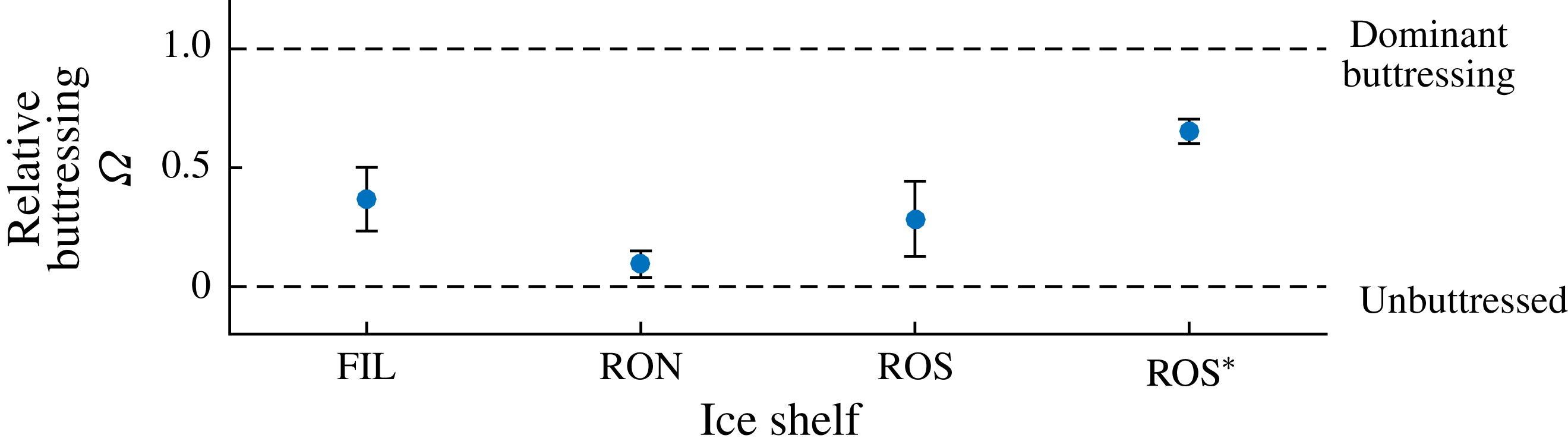
1 Introduction
Understanding the mechanics of marine ice sheets – those that lie predominantly submerged in the ocean – is vitally important if we are to predict contributions to future sea level with any confidence. The West Antarctic Ice Sheet (WAIS) is a continent-scale marine ice sheet that sits on bedrock at an average depth of one kilometre below sea level (Bamber et al. Reference Bamber, Riva, Vermeersen and LeBrocq2009). The total or partial collapse of the WAIS as a consequence of its detachment from the bedrock under buoyancy has the potential to outstrip other contributions to global sea-level rise over the course of the next few centuries (Hanna et al. Reference Hanna, Navarro, Pattyn, Domingues, Fettweis, Ivins, Nicholls, Ritz, Smith, Tulaczyk, Whitehouse and Zwally2013). Recent unprecedented thinning and retreat of its constituent Pine Island and Thwaites Glaciers may be independently contributing as much as 6 % of the present total rate of global sea-level rise. However, the future contributions of the WAIS are uncertain owing to significant challenges in characterising and parametrising the phenomena controlling its evolution. A potentially dominant phenomenon is an effect of the peripheral floating regions of the ice sheet – the ice shelves – in creating a buttress that protects the considerably larger grounded interior against surging outwards into the ocean. The role of this effect in controlling the future of the WAIS is presently an open question. This paper and its companion will explore the influence of lateral stresses and ice-shelf buttressing, and elucidate the critical conditions under which it protects a marine ice sheet from triggering runaway buoyancy-driven collapse.
Concerns over the essential stability of the WAIS are rooted in the hypothesis of the marine ice sheet instability (MISI). Simply put, a grounding-line retreat driven by buoyancy has the potential to manifest rapidly and with irreversible change, particularly for regions where the underlying bedrock slopes upwards in the direction of flow (a positive slope) (Weertman Reference Weertman1974; Thomas & Bentley Reference Thomas and Bentley1978). The runaway retreat of a grounding line underlying the MISI principle can be motivated on the basis of an increasing relationship between the grounding-line thickness and the rate of thinning of ice at the grounding line. Much of the bedrock underlying the WAIS deepens towards the centre of the continent owing to isostatic depression, creating prevailing regions of positive bed slope. If a grounding line retreats on a positive bed slope then, since it moves into deeper water, the larger buoyancy forces act to stimulate a yet faster retreat, producing a positive feedback. The potential for this positive feedback has led to the hypothesis that regions of the WAIS may collapse rapidly across parametric ‘tipping points’. It has been suggested that ice-shelf buttressing may be necessary to suppress a potential full-scale or regional collapse of the WAIS (Hughes Reference Hughes1981; Stuiver et al. Reference Stuiver, Denton, Hughes and Fastook1981).
The viscous creep of marine ice sheets can be modelled using a system of thin-film viscous flow equations known as the shallow-stream or shallow-shelf approximation (SSA). The equations describe the interactions between gravitational stresses, basal drag stresses and extensional (stretching) stresses under a shear-thinning flow model (e.g. Morland Reference Morland1987; MacAyeal Reference MacAyeal1989). In situations where the ice shelf undergoes unconfined, horizontally one-dimensional flow, these equations predict that the hydrostatic pressure of the ocean simply transmits directly through the ice shelf to the grounding line (MacAyeal & Barcilon Reference MacAyeal and Barcilon1988; Chugunov & Wilchinsky Reference Chugunov and Wilchinsky1996; Wilchinsky & Chugunov Reference Wilchinsky and Chugunov2000; Schoof Reference Schoof2007a ,Reference Schoof b ; Robison, Huppert & Worster Reference Robison, Huppert and Worster2010; Tsai, Stewart & Thompson Reference Tsai, Stewart and Thompson2015). The removal of a one-dimensional ice shelf thus has no influence on the dynamics of the grounding line. The only resistance to flow across the grounding line in this case stems from the longitudinal extensional (stretching) stresses associated with the non-Newtonian creep of ice near the front of the grounded region. In light of this simplification, it follows that the rate of extension, and hence the rate of thinning, at an unbuttressed grounding line is controlled by the hydrostatic pressure drop between the front of the grounded region and the ocean in front of it, indicating the potential for runaway feedback between thinning and retreat on a positive bed slope. This mechanism can be embodied within a relationship between the flux and thickness at an unbuttressed grounding line derived from a scaling analysis of the steady-state equations (e.g. Chugunov & Wilchinsky Reference Chugunov and Wilchinsky1996; Wilchinsky & Chugunov Reference Wilchinsky and Chugunov2000; Schoof Reference Schoof2007a ,Reference Schoof b ). By applying this flux relationship in the context of a time-dependent marine ice sheet under suitable approximations (Schoof Reference Schoof2007a ,Reference Schoof b ), it can be argued that the retreat of the grounding line on a positive bed slope increases the flux across the grounding line, consistent with a mechanism of positive feedback between increasing flux and grounding-line retreat. Grounding lines can therefore transition to positive-feedback retreat, leading to rapid and potentially permanent changes in grounding-line positions (Schoof Reference Schoof2007a ).
However, observational evidence and the results of numerical simulations have indicated that a number of properties of one-dimensional flow do not hold as a consequence of two-dimensional stresses generated by lateral contact. A significant proportion of the ice shelves surrounding Antarctica are confined by rock or near-stationary ice, resulting in lateral-drag forces, which accumulate to generate a buttressing force that provides a direct resistive force, additional to the extensional stress, that suppresses flow across the grounding line. The effect was demonstrated by the significant accelerations of feeding ice streams following the collapse of the Larson B Ice Shelf (Rignot et al. Reference Rignot, Casassa, Gogineni, Krabill, Rivera and Thomas2004; Scambos et al. Reference Scambos, Bohlander, Shuman and Skvarca2004), accelerations which are also illustrated by simulations of this configuration (de Rydt et al. Reference de Rydt, Gudmundsson, Rott and Bamber2015). Two-dimensional modelling of the SSA equations (e.g. MacAyeal Reference MacAyeal1989; Goldberg, Holland & Schoof Reference Goldberg, Holland and Schoof2009; Gagliardini et al. Reference Gagliardini, Durand, Zwinger, Hindmarsh and Meur2010; Gudmundsson et al. Reference Gudmundsson, Krug, Durand, Favier and Gagliardini2012; Gudmundsson Reference Gudmundsson2013; Favier et al. Reference Favier, Durand, Cornford, Gudmundsson, Gagliardini, Gillet-Chaulet and Brocq2014) has indicated the significance of a buttressing ice shelf and, in turn, the melting and calving rates that control its magnitude. An interesting conclusion is that buttressing can allow a grounding line to settle stably on a positive bed slope (Goldberg et al. Reference Goldberg, Holland and Schoof2009; Gudmundsson et al. Reference Gudmundsson, Krug, Durand, Favier and Gagliardini2012), deviating qualitatively from one-dimensional predictions. Idealised radially flowing marine ice sheets, in which buttressing is generated by viscous hoop stresses, also leads to stabilisation on non-negative slopes (Pegler & Worster Reference Pegler and Worster2012, Reference Pegler and Worster2013).
The effects of ice-shelf buttressing from lateral stresses can also be encapsulated within so-called flow-line models, which form a mathematically one-dimensional system of equations in which lateral drag stresses are incorporated in the form of a Navier-type drag law (e.g. van der Veen Reference van der Veen1999; Dupont & Alley Reference Dupont and Alley2005; Nick et al. Reference Nick, van der Veen, Vieli and Benn2010; Hindmarsh Reference Hindmarsh2012; Pegler et al. Reference Pegler, Kowal, Hasenclever and Worster2013; Walker et al. Reference Walker, Holland, Parizek, Alley, Nowicki and Jenkins2013; Kowal, Pegler & Worster Reference Kowal, Pegler and Worster2016; Pegler Reference Pegler2016; Schoof, Davis & Popa Reference Schoof, Davis and Popa2017). The model incorporates the effect of lateral stresses within a framework that yields considerably faster numerical implementation than the full SSA equations, eases the physical interpretation of results and creates analytical and asymptotic inroads. The development of analytical inroads has been demonstrated in the context of a steady-state ice shelf (Pegler Reference Pegler2016), where it is determined that the floating component can be integrated to yield exact or asymptotic solutions describing the structure of a buttressing ice shelf. Across the spectrum of relative buttressing strength, the solutions were determined to undergo a transition from the broadly concave solution describing a non-buttressing ice shelf (van der Veen Reference van der Veen1983), which has no sensitivity to its downstream calving position, to a regime containing a prevailing internal section of relatively milder slope that is controlled to leading order by the calving position. The connection between the prevailing internal region and the grounding line takes place through a short transitional boundary layer in which the divergence of extensional stresses attains magnitudes several orders larger than elsewhere in the ice sheet as the flow adjusts to the lateral-stress-dominated regime. The boundary layer is distinct from the extensional boundary layer of the kind discussed in the context of the grounded region upstream of the grounding line (cf. Schoof Reference Schoof2007b ) and involves considerably larger gradients in extensional stresses. For a narrow geometry, a more reduced, nonlinear diffusive form of a flow-line model of a marine ice sheet can be formulated (Pegler et al. Reference Pegler, Kowal, Hasenclever and Worster2013) in which buttressing provides the dominant resistance to flow across the grounding line and the migration of the grounding line is controlled by the time-dependent evolution of the ice shelf. Since the rate of thickening of the ice shelf is independent of the basal slope, it is clear from the perspective of this reduced model that the possibility of a grounding line to form a stable steady state does not depend on the local basal gradient. Across the spectrum of aspect ratios, there is thus a complete switch in the control of a grounding line from being insensitive to the ice shelf to being entirely controlled by it. In a recent study, Schoof et al. (Reference Schoof, Davis and Popa2017) consider a flow-line model in which the control of a grounding line is examined subject to two alternative calving laws different to the case of a direct imposition (e.g. Goldberg et al. Reference Goldberg, Holland and Schoof2009; Gudmundsson et al. Reference Gudmundsson, Krug, Durand, Favier and Gagliardini2012). This includes a consideration of the case of a tidewater glacier with no ice-shelf buttressing but with lateral stresses in the grounded region, which are found to affect the relationship between thickness and flux at the grounding line. The second is the situation where an ice shelf forms and calves under a hydrofracture model (Nick et al. Reference Nick, van der Veen, Vieli and Benn2010), which, for steady-state analysis, can be reduced to the imposition of a calving thickness. The results show that a stable grounding line is possible in this case on a retrograde slope despite the loss of a necessary relationship between grounding-line retreat and increasing buttressing.
The present study extends the analytical results for steady-state solutions and buttressing forces given by Pegler (Reference Pegler2016) to the context of a full ice-sheet model and explores the dominant flow balances, regimes and ice-sheet flow structures that arise. The aim is to investigate the variation in these properties across the spectrum of relative buttressing strength bridging the unbuttressed limit (Schoof Reference Schoof2007b ) to the limit of strong buttressing (Pegler et al. Reference Pegler, Kowal, Hasenclever and Worster2013). An overarching objective is to clarify the fundamental switches in dynamical characteristics and parameter controls resulting from the introduction of lateral stresses. By incorporating the buttressing stress resulting from the steady-state integration (Pegler Reference Pegler2016), an algebraic equation for buttressed grounding lines is obtained that allows for a rapid determination of steady states without the need for any consideration of a differential equation. These results differ in methodology from the kind of analysis based on direct numerical solution of a flow-line model (e.g. Dupont & Alley Reference Dupont and Alley2005; Nick et al. Reference Nick, van der Veen, Vieli and Benn2010; Pegler et al. Reference Pegler, Kowal, Hasenclever and Worster2013; Walker et al. Reference Walker, Holland, Parizek, Alley, Nowicki and Jenkins2013; Schoof et al. Reference Schoof, Davis and Popa2017). Relationships between the force balances and the asymptotic structure of the ice shelf are investigated, with the finding that buttressing is linked to three specific thicknesses defining the structure of the ice shelf: the grounding-line thickness, the calving thickness and the thickness in front of the input boundary layer of the ice shelf. It is shown that the grounding line can be set directly by the prevailing profile of the ice shelf (Pegler Reference Pegler2016), elucidating a complete switch in the mechanical role of the ice shelf between weak and strong buttressing from having no control to having a completely independent control of the grounding line. It will be explained why lateral stresses specifically in ice shelves – even if orders of magnitude smaller than resistive stresses in the grounded region – have such a major role in maintaining ice-sheet stability. The flow-line predictions and the reduced analytical predictions are benchmarked against direct numerical simulations of the full two-dimensional SSA equations (Gudmundsson et al. Reference Gudmundsson, Krug, Durand, Favier and Gagliardini2012), with limitations discussed. The configurations are also shown to partition between consistent steady-state solutions with a continuously floating ice shelf (for which the reduced analytical theory applies) and those where lateral stresses in the ice shelf are sufficient to induce it to reground downstream of the primary grounding line. The generation and sustainment of ice rises is thus linked to the sustainment of lateral stresses. The critical prediction of regrounding can result in considerably greater buttressing than the direct non-local integration of lateral stresses along the ice shelf, and is shown to produce a rich variety of additional steady-state solutions than predicted by the simplest forms of the analytical theory. The potential for lateral stresses to eliminate hysteresis effects is discussed.
I begin in § 2 by developing the quasi-two-dimensional marine ice sheet model from first principles, corroborating its predictions against full SSA equations and discussing its limitations. An overview of the time-dependent phenomena is provided in § 3. This is followed in § 4 with a development of the reduced analytical descriptions of steady-state grounding-line forces, and a discussion of the fundamental differences between unbuttressed and buttressed grounding-line dynamics. Section 5 details the effects of lateral stresses on the structure of a marine ice sheet. Section 6 discusses the concurrent phenomenon of ‘secondary grounding’ whereby lateral stresses induce further contacts between an ice shelf and the bedrock. The theory is demonstrated in § 7 for an illustrative nonlinear bedrock topography. The implications of the results to the geophysical context are described in § 8. The key conclusions are summarised in § 9.
2 Theoretical development
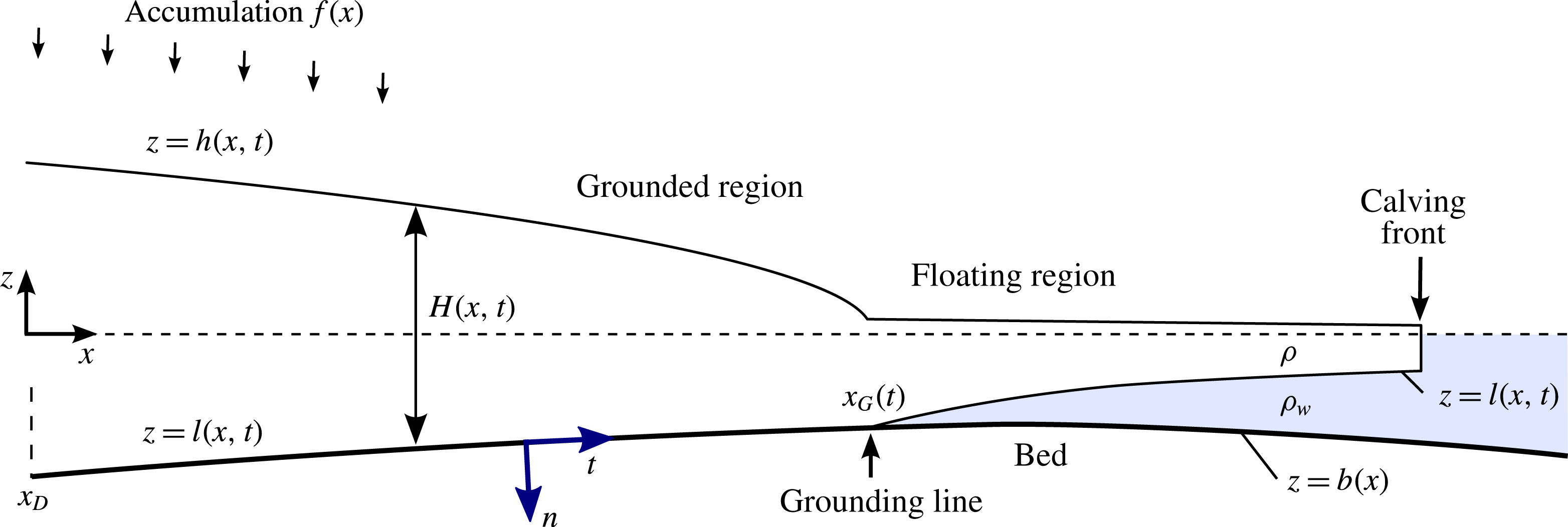
Consider a marine ice sheet comprising a viscous, incompressible fluid layer (ice) of density
 $\unicode[STIX]{x1D70C}$
flowing over a rigid bed
 $z=b(x)$
and lying submerged in an effectively inviscid fluid (the ocean) of larger density
 $\unicode[STIX]{x1D70C}_{w}$
and upper surface
 $z=0$
(figure 1). The domain of the ice sheet is assumed to extend from a line symmetry or ice divide at
 $x_{D}$
to a termination or calving front
 $x_{C}$
. The ice sheet has a free upper surface
 $z=h(x,t)$
and a partially floating, partially grounded lower surface
 $z=l(x,t)$
. Let the vertical thickness distribution of the ice sheet be denoted
 $H(x,t)\equiv h(x,t)-l(x,t)$
. A marine ice sheet comprises two regions: the upstream grounded region, wherein
 $l=b$
, and the downstream ice shelf or floating region, wherein
 $l>b$
. The grounded and floating regions connect at the grounding line
 $x=x_{G}(t)$
.
Schematic cross-section of a marine ice sheet.
Plans showing (a) an ice shelf calving exterior to its region of confinement, and (b) interior to it. The grounding line is illustrated by a solid red curve. In (a), lateral stresses terminate at the detachment points of the ice shelf near the channel mouth. For this case, the detachment point determines where condition (2.15) is applied. For (b), equation (2.15) is imposed directly at the calving front itself.
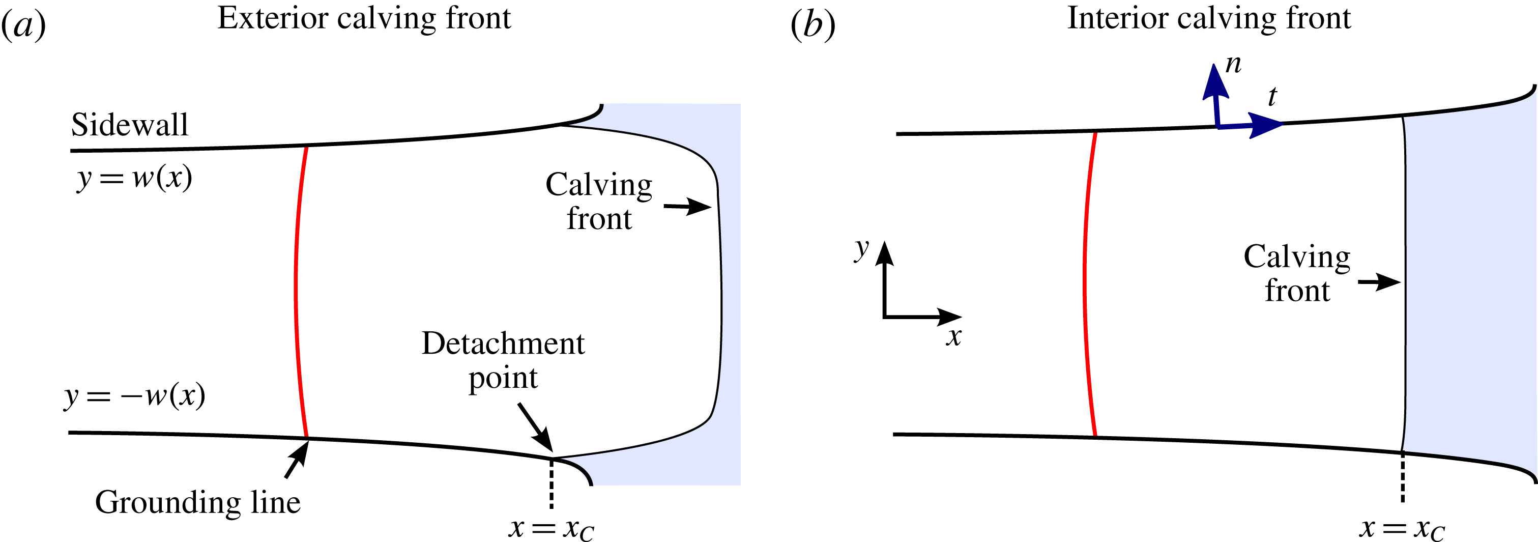
The flow is confined laterally between margins along
 $y=\pm w(x)$
, representing either rock or near-stationary grounded ice, as illustrated in the planform schematics of figure 2. The calving front (terminus) of the ice shelf can either lie exterior to the confining region (figure 2
a) or interior to it (figure 2
b). In the former case, the ice shelf fills the channel fully and detaches from the boundaries at or near the channel exit, as is characteristic of some ice shelves (e.g. the Amery Ice Shelf). For the case of interior calving, the ice shelf instead calves without detaching, a feature characteristic of Pine Island Glacier, for example. Interior and exterior calving introduce slightly different modelling considerations, which will be detailed in § 2.1.
The equations of momentum and mass conservation governing the viscous flow are
 $$\begin{eqnarray}\displaystyle \unicode[STIX]{x1D735}\boldsymbol{\cdot }\unicode[STIX]{x1D748}-\unicode[STIX]{x1D70C}g\hat{\boldsymbol{z}}=\mathbf{0},\quad \unicode[STIX]{x1D735}\boldsymbol{\cdot }\boldsymbol{u}=0, & & \displaystyle\end{eqnarray}$$
where
 $\unicode[STIX]{x1D735}$
is the gradient operator,
 $\boldsymbol{u}(\boldsymbol{x},t)$
is the three-dimensional velocity of the flow,
 $\unicode[STIX]{x1D748}\equiv -p\unicode[STIX]{x1D644}+\unicode[STIX]{x1D749}$
is the stress tensor,
 $p$
is the pressure,
 $\unicode[STIX]{x1D749}=2\unicode[STIX]{x1D707}\unicode[STIX]{x1D65A}$
is the deviatoric stress tensor,
 $\unicode[STIX]{x1D707}(\boldsymbol{x},t)$
is the effective viscosity,
 $\unicode[STIX]{x1D65A}\equiv (1/2)[\unicode[STIX]{x1D735}\boldsymbol{u}+(\unicode[STIX]{x1D735}\boldsymbol{u})^{\text{T}}]$
is the strain-rate tensor,
 $\hat{\boldsymbol{z}}$
is the vertical unit vector and
 $g$
is the gravitational strength. In accordance with Glen’s law, I allow for a viscous power-law fluid defined by the relationship for the effective viscosity
 $$\begin{eqnarray}\unicode[STIX]{x1D707}=\unicode[STIX]{x1D707}_{0}\left({\textstyle \frac{1}{2}}\unicode[STIX]{x1D65A}\boldsymbol{ : }\unicode[STIX]{x1D65A}\right)^{[(1/n)-1]/2}\equiv \unicode[STIX]{x1D707}_{0}\left({\textstyle \frac{1}{2}}\unicode[STIX]{x1D65A}\boldsymbol{ : }\unicode[STIX]{x1D65A}\right)^{(m-1)/2},\end{eqnarray}$$
where
 $\unicode[STIX]{x1D707}_{0}$
is the coefficient of viscosity,
 $n$
the power-law exponent and
 $m\equiv 1/n$
(Cuffey & Paterson Reference Cuffey and Paterson2010). For glacial flow, the shear-thinning case
 $n=3$
[
 $m=1/3$
] is most commonly assumed, and
 $\unicode[STIX]{x1D707}_{0}\sim 10^{8}~\text{Pa}~\text{s}^{1/n}$
is representative.
The zero-stress condition along the free top surface of the ice sheet is given by
 $$\begin{eqnarray}\boldsymbol{n}\boldsymbol{\cdot }\unicode[STIX]{x1D748}=\mathbf{0}\quad \text{on }z=h(x,t),\end{eqnarray}$$
where
 $\boldsymbol{n}$
is the unit outward normal to the surface.
The base of the ice sheet is subject to different conditions depending on whether it is grounded or floating. In the grounded region, I apply the Weertman drag law (a nonlinear Navier condition),
 $$\begin{eqnarray}\boldsymbol{t}\boldsymbol{\cdot }\unicode[STIX]{x1D748}\boldsymbol{\cdot }\boldsymbol{n}=\unicode[STIX]{x1D70F}_{b}(\boldsymbol{t}\boldsymbol{\cdot }\boldsymbol{u})=C_{-}(\boldsymbol{t}\boldsymbol{\cdot }\boldsymbol{u})^{m_{-}}\quad \text{on }z=l(x,t)=b(x),\end{eqnarray}$$
where
 $\boldsymbol{t}$
and
 $\boldsymbol{n}$
are the unit tangent and normal to the lower surface,
 $C_{-}$
is the basal-drag coefficient and
 $m_{-}$
is the basal drag-law exponent. Models of this kind are standard in ice-sheet simulation, and aim to parametrise processes of glacial slip, such as regelation and sliding over rough bedrock (Weertman Reference Weertman1957; Lliboutry Reference Lliboutry1987; Gudmundsson Reference Gudmundsson1997). It is usual to identify the slip-law exponent with the rheological exponent,
 $m_{-}=m$
, which is the case commonly applied in modelling the water-lubricated ice streams that typically feed ice shelves. Here, I will focus the examples on cases where
 $m_{-}=m$
and
 $C_{-}$
is uniform. Drag coefficients of
 $C_{-}=10^{5}{-}10^{6}~\text{Pa}~(\text{m}~\text{s}^{-1})^{-m_{-}}$
are representative (Cuffey & Paterson Reference Cuffey and Paterson2010). These drag coefficients are sufficiently small that the velocity profile of an ice stream is free of vertical shear to leading order (
 $\boldsymbol{u}\approx \boldsymbol{u}(x,y,t)$
only).
The floating region has a free lower boundary, which differs mechanically from the grounded region in being both geometrically unconstrained and subject to negligible tangential stresses from the ocean below it. Assuming a purely hydrostatic ocean pressure,
 $p_{w}=-\unicode[STIX]{x1D70C}_{w}gz$
, I impose continuity of stress along the base of the floating region with
 $$\begin{eqnarray}\boldsymbol{n}\boldsymbol{\cdot }\unicode[STIX]{x1D748}=-p_{w}\boldsymbol{n}=\unicode[STIX]{x1D70C}_{w}gl\boldsymbol{n}\quad \text{on }z=l(x,t)>b(x).\end{eqnarray}$$
The new effects explored in this paper stem from the drag forces exerted by the lateral margins,
 $y=\pm w(x)$
. Velocimetric observations (Rignot, Mouginot & Scheuchl Reference Rignot, Mouginot and Scheuchl2011) indicate that a no-slip condition,
 $\boldsymbol{u}=\mathbf{0}$
, may be the most widely relevant condition at ice-shelf margins. However, localised softening or damage may in principle lead to more slip-like behaviour in ice streams and ice shelves. For any of these cases, a drag law of the form
 $$\begin{eqnarray}\boldsymbol{t}\boldsymbol{\cdot }\unicode[STIX]{x1D748}\boldsymbol{\cdot }\boldsymbol{n}=\unicode[STIX]{x1D70F}_{s}\quad \text{on }y=\pm w(x)\end{eqnarray}$$
can be proposed, where
 $\unicode[STIX]{x1D70F}_{s}$
is the lateral stress. A specific model for
 $\unicode[STIX]{x1D70F}_{s}$
will be discussed below. Some previous modelling studies (e.g. MacAyeal Reference MacAyeal1989) prescribe
 $\unicode[STIX]{x1D70F}_{s}$
directly, but this does not describe the viscous resistance to shearing of the flow consistently.
Assuming sufficiently weak basal drag, equation (2.1a,b ) can be depth integrated to yield a simplified system of thin-film viscous flow equations commonly referred to as the ‘shallow-stream’ or ‘shallow-shelf’ approximation (SSA), which are provided in the supplementary document (https://doi.org/10.1017/jfm.2018.741) (see DiPietro & Cox (Reference DiPietro and Cox1979), MacAyeal (Reference MacAyeal1989) or Pegler & Worster (Reference Pegler and Worster2012) for alternative derivations of these equations).
The first of two thin-flow simplifications underlying this model is that the leading-order vertical stress is hydrostatic,
 $\unicode[STIX]{x1D70E}_{zz}=\unicode[STIX]{x1D70C}g(h-z)$
. Under this approximation, the height in floating regions conforms to Archimedes’ principle of flotation,
 $h=(\unicode[STIX]{x0394}\unicode[STIX]{x1D70C}/\unicode[STIX]{x1D70C}_{w})H$
. For the grounded region, the trivial relationship of
 $h=b+H$
applies instead. The thickness and upper-surface height can generally be related by the conditional expression
 $$\begin{eqnarray}h=\left\{\begin{array}{@{}ll@{}}b+H & \text{if }H>d(x)\quad (\text{grounded region}),\\ (\unicode[STIX]{x0394}\unicode[STIX]{x1D70C}/\unicode[STIX]{x1D70C}_{w})H & \text{if }H<d(x)\quad (\text{floating region}).\end{array}\right.\end{eqnarray}$$
The function
 $d(x)\equiv -(\unicode[STIX]{x1D70C}_{w}/\unicode[STIX]{x1D70C})b(x)$
is referred to as the flotation profile. A grounding line
 $x_{G}(t)$
occurs where the ice thickness
 $H(x,t)$
and flotation profile
 $d(x)$
coincide, giving the flotation condition
 $$\begin{eqnarray}H(x_{G},t)=d(x_{G})\equiv -(\unicode[STIX]{x1D70C}_{w}/\unicode[STIX]{x1D70C})b(x_{G}).\end{eqnarray}$$
The second simplification is the depth- and width-integrated form of the longitudinal,
 $x$
-component of the Stokes’ equation (2.1a
), which I write as
 $$\begin{eqnarray}\underbrace{\frac{\unicode[STIX]{x2202}}{\unicode[STIX]{x2202}x}\left(4wH\unicode[STIX]{x1D707}\frac{\unicode[STIX]{x2202}u}{\unicode[STIX]{x2202}x}\right)}_{\substack{ \text{Extensional} \\ \text{stress}}}-\underbrace{\frac{}{}H\unicode[STIX]{x1D70F}_{s}(u)}_{\substack{ \text{Lateral} \\ \text{stress}}}-\underbrace{\frac{}{}w\unicode[STIX]{x1D70F}_{b}(u)}_{\substack{ \text{Basal} \\ \text{stress}}}=\underbrace{\unicode[STIX]{x1D70C}gwH\frac{\unicode[STIX]{x2202}h}{\unicode[STIX]{x2202}x}}_{\substack{ \text{Gravitational} \\ \text{force}}},\end{eqnarray}$$
where the effective viscosity
 $\unicode[STIX]{x1D707}=\unicode[STIX]{x1D707}_{0}|\unicode[STIX]{x2202}u/\unicode[STIX]{x2202}x|^{m-1}$
. This equation is equivalent to the one-dimensional form of a standard ice-stream model (e.g. Muszynski & Birchfield Reference Muszynski and Birchfield1987; MacAyeal Reference MacAyeal1989), except augmented to include the drag force owing to lateral stresses
 $\unicode[STIX]{x1D70F}_{s}$
.
The direct incorporation of basal stress
 $\unicode[STIX]{x1D70F}_{b}$
within the one-dimensional extensional flow model (2.9) can be justified formally on the basis of a leading-order vertical plug flow arising from sufficient basal lubrication. By analogy, the direct incorporation of lateral stress
 $\unicode[STIX]{x1D70F}_{s}$
within (2.9) could be justified, at least mathematically, on the basis of an assumption that lateral stresses are much smaller than the stress associated with shearing transversely across the channel, i.e.
 $$\begin{eqnarray}\unicode[STIX]{x1D70F}_{s}\ll \unicode[STIX]{x1D70F}_{s}^{shear}\equiv \unicode[STIX]{x1D707}_{0}(w^{-1}u)^{m},\end{eqnarray}$$
where
 $\unicode[STIX]{x1D70F}_{s}^{shear}$
is the intrinsic scale of transverse shear stress that would arise for a condition of no lateral slip. In this limit of weak lateral drag, the flow is transversely plug-like to leading order. While considerable softening of ice (e.g. by viscous heating) may theoretically allow for this limit, I anticipate that the more broadly relevant case for an ice shelf is a no-slip condition. However, this entails
 $\unicode[STIX]{x1D70F}_{s}\sim \unicode[STIX]{x1D70F}_{s}^{shear}$
, and thus does not satisfy any asymptotic condition that might allow for the incorporation of the lateral stress
 $\unicode[STIX]{x1D70F}_{s}$
into the width-integrated formulation (2.9) to be justified in any general asymptotic limiting sense. In principle, all components of the horizontal stress tensor may become important in either the stress divergence or the determination of the effective viscosity
 $\unicode[STIX]{x1D707}$
through different regions of the flow. On this basis, it might be anticipated that explicit two-dimensional modelling is necessarily in order to accommodate the effects of zero lateral slip in marine ice sheets (e.g. Gudmundsson et al.
Reference Gudmundsson, Krug, Durand, Favier and Gagliardini2012). Nevertheless, it will be demonstrated below that the shear stress for no lateral slip can, under situations to be discussed, be modelled accurately by applying the heuristic shear-drag parametrisation
 $$\begin{eqnarray}\displaystyle \unicode[STIX]{x1D70F}_{s}=\unicode[STIX]{x1D707}_{0}(\unicode[STIX]{x1D706}_{+}^{-1}\bar{u})^{m}\equiv C_{+}\bar{u}^{m}\quad \text{where}~\unicode[STIX]{x1D706}_{+}=\unicode[STIX]{x1D706}_{+}^{soft}+\frac{w}{2^{n-1}(n+2)} & & \displaystyle\end{eqnarray}$$
is an ‘effective slip length’ representing the sum of a ‘softening slip length’
 $\unicode[STIX]{x1D706}_{+}^{soft}$
and a cross-channel average slip associated with a local approximation of plane (two-dimensional) Poiseuille flow (Pegler Reference Pegler2016). Here, the overbar denotes the width average
 $$\begin{eqnarray}\bar{u}(x,t)\equiv \frac{1}{2w}\int _{-w}^{w}u(x,y,t)\,\text{d}y.\end{eqnarray}$$
The term
 $\unicode[STIX]{x1D706}_{+}^{soft}$
is included here to represent a possible effect of lateral softening and will be neglected henceforth. A similar expression to (2.11) based on centreline velocity is used by Hindmarsh (Reference Hindmarsh2012) for the purpose of a scaling analysis with a different prefactor. While appropriate for
 $u$
interpreted as the centreline velocity and sufficient for the scaling analysis, the form given there leads to an inconsistency with the width-integrated mass-conservation equation (2.18) that does not arise with the prefactor of (2.11b
). The shear-drag parametrisation (2.11) is applied here as an explicit closure condition within the context of solving a full mathematical model, and will be benchmarked against the full SSA model. The model formed by combining (2.9) and the parametrisation (2.11) will be referred to as the quasi-two-dimensional (Q2D) model.
As noted above, the model of (2.11) is not based on any asymptotic approximation. The relationship depends in particular on neglecting the longitudinal extensional stress in formulating (2.11) despite its retainment in the force-balance equation (2.9). For
 $n\neq 1$
, the model also depends on the neglect of transverse shear stress in the expression for the effective viscosity
 $\unicode[STIX]{x1D707}$
in the term representing the divergence of extensional stresses, namely, the first term of (2.9). Despite the neglect of these contributions, the model does, by design, consistently recover both the purely extensional (wide) and the transverse-shear-dominated (narrow) limits (Pegler Reference Pegler2016). However, an ice shelf will naturally undergo transitional balances involving mixtures of these stresses, particularly in the immediate front of a grounding line (Pegler Reference Pegler2016). It is possible, at least in principle, for the model to be less accurate in such regions. In order to reveal any significant disparities, I conducted a series of numerical benchmarks against the full, unsimplified two-dimensional thin-flow (SSA) equations for
 $n=3$
applied across a wide spectrum of planform aspect ratios and compared the results with the predictions of the Q2D model defined by (2.9) and (2.11). As reported in the supplementary document, excellent agreement is generally found across the complete range of aspect ratios. The best relative agreement occurs for wide embayments and a slight discrepancy applies for the narrow limit. Just two localised regions of the flow exhibit minor discrepancies. One is the so-called input boundary layer of the ice shelf immediately in front of the grounding line (Pegler Reference Pegler2016). The other is near the calving front, where the corner singularity at the margins causes the transverse velocity to become large. It should be noted that the comparisons provided in the supplementary results focus on the case of a uniform width. It is likely that abrupt transitions from narrow ice streams to wide ice shelves will involve additional stresses not described by the Q2D model. Subject to this caveat and others summarised in § 8.3, the analytical framework provided by (2.9) and (2.11) provides a good description of the dynamics of outlet systems spanning narrow to wide embayments.
For small lateral softening,
 $\unicode[STIX]{x1D706}_{+}^{soft}\ll w$
, the effective slip length
 $\unicode[STIX]{x1D706}_{+}$
defined by (2.11b
) is a scaled surrogate for the channel half-width
 $w$
. For example,
 $n=3$
yields
 $\unicode[STIX]{x1D706}_{+}\approx w/20$
. For representative values of
 $w=20$
–200 km,
 $\unicode[STIX]{x1D706}_{+}\approx 1$
–10 km. The associated effective lateral-drag coefficient
 $C_{+}=10^{6}{-}10^{7}~\text{Pa}~(\text{m}~\text{s}^{-1})^{-m}$
is much larger than the upper bound of the typical values of the basal-drag coefficient given above. Therefore, as expected, the lateral condition in an ice shelf generates more shear (i.e. is ‘harder’) than the basal condition in the grounded ice stream. The relative significance of basal stress compared to lateral drag, as described by (2.9), is measured by the ratio of the width-integrated basal drag
 $2w\unicode[STIX]{x1D70F}_{b}$
to the sum of the two depth-integrated lateral-drag stresses from the margins,
 $2H\unicode[STIX]{x1D70F}_{s}$
, namely,
 $$\begin{eqnarray}\displaystyle R\equiv \frac{2w\unicode[STIX]{x1D70F}_{b}}{2H\unicode[STIX]{x1D70F}_{s}}=\frac{wC_{-}}{HC_{+}}=\left\{\begin{array}{@{}ll@{}}1{-}100 & \text{if }H>d(x)\quad (\text{grounded region}),\\ 0 & \text{if }H<d(x)\quad (\text{floating region}).\end{array}\right. & & \displaystyle\end{eqnarray}$$
It should be noted that the basal stress is modelled using a prescribed drag coefficient
 $C_{-}$
, while the lateral stresses in the ice shelf, being shear dominated, is controlled geometrically by the half width,
 $\unicode[STIX]{x1D706}_{+}\propto w$
. The dimensionless basal strength
 $R$
thus involves a mixture of the transverse aspect ratio and the ratio of drag coefficients. In view of the considerable lubrication typical at the base of an ice stream, it is possible for the overall effect of lateral stresses to be comparable to that of basal stress despite the much shorter length scale (the glacier’s height) over which they are applied compared to the basal stress. The estimates of
 $R$
in the grounded regions (2.13a
) follow from the ranges of values of
 $C_{-}$
and
 $C_{+}$
given above and typical thickness scales of
 $H\sim 10^{2}$
–
 $10^{3}$
m. The prediction that
 $R\gtrsim 1$
indicates that the overall effect of basal drag in the ice stream is comparable to or larger than the lateral drag. It is important to note that, irrespective of the relative magnitude of lateral stress in the grounded region, the lateral stresses in the ice shelf have a central role in ice-sheet stability. This is because the force against which they compete for significance is not the basal stress but the extensional stress resisting flow across the grounding line (the only resistance to flow across the grounding line in the absence of buttressing). The magnitude of the extensional stress can become readily matched and/or exceeded by the buttressing force generated by lateral stresses through the length of the ice shelf. A sufficient resistance to flow across a grounding line forms an independent necessary condition for maintaining a large ice sheet. Thus, in providing a potentially dominant contribution to this resistance, lateral stresses exerted in the ice shelf, even if relatively small compared to the lateral and basal stresses upstream of the grounding line or exerted over a relatively short ice shelf, have the potential to dominate control of the large-scale mass balance.
Using (2.5) and (2.6) to substitute for the drag laws
 $\unicode[STIX]{x1D70F}_{b}(u)$
and
 $\unicode[STIX]{x1D70F}_{s}(u)$
in (2.9), dropping the overbars and using (2.7) to substitute for the surface height
 $h$
in favour of the thickness
 $H$
, I obtain
 $$\begin{eqnarray}\displaystyle 4\frac{\unicode[STIX]{x2202}}{\unicode[STIX]{x2202}x}\left(\unicode[STIX]{x1D707}wH\frac{\unicode[STIX]{x2202}u}{\unicode[STIX]{x2202}x}\right)=\left\{\begin{array}{@{}ll@{}}\displaystyle (C_{-}w+C_{+}H)u^{m}+\unicode[STIX]{x1D70C}gwH\left(\frac{\unicode[STIX]{x2202}H}{\unicode[STIX]{x2202}x}+\frac{\text{d}b}{\text{d}x}\right) & \text{if }H>d(x),\\ \displaystyle C_{+}Hu^{m}+\unicode[STIX]{x1D70C}g^{\prime }wH\frac{\unicode[STIX]{x2202}H}{\unicode[STIX]{x2202}x} & \text{if }H<d(x),\end{array}\right. & & \displaystyle\end{eqnarray}$$
where
 $g^{\prime }\equiv (\unicode[STIX]{x1D70C}_{w}-\unicode[STIX]{x1D70C})g/\unicode[STIX]{x1D70C}_{w}$
is a reduced gravity. Equation (2.14) is a generalisation of one-dimensional ice-sheet models to allow for lateral drag (
 $C_{+}=0$
recovers the unbuttressed case). As discussed above, the key new effects stem from the lateral stress exerted in the floating component, given by the first term on the right-hand side of (2.14b
).
2.1 Dynamic condition at the calving front or detachment location
Whether the calving front of the ice shelf lies exterior to its embayment (exterior calving) or interior to it (interior calving), the lateral stresses will cease to be exerted beyond a position denoted
 $x_{C}$
. These two situations are illustrated respectively in figure 2(a,b). Exterior calving characterises the Amery Ice Shelf, for example. Interior calving characterises the Ross and Filchner–Ronne ice shelves. For exterior calving, I identify
 $x_{C}$
as the position of detachment of the ice shelf from the lateral boundaries (a position coincident with the mouth of an outlet channel, as illustrated by experiments in Pegler Reference Pegler2016). For interior calving, I identify
 $x_{C}$
as the calving front itself.
At
 $x_{C}$
, I impose the stress condition
 $$\begin{eqnarray}\unicode[STIX]{x1D707}\frac{\unicode[STIX]{x2202}u}{\unicode[STIX]{x2202}x}=\frac{\unicode[STIX]{x1D70C}g^{\prime }}{8}H\quad \text{at }x=x_{C}.\end{eqnarray}$$
For interior calving,
 $x_{C}$
depends on the calving processes that control the calving position. By treating
 $x_{C}$
as a parameter (cf. Gudmundsson et al.
Reference Gudmundsson, Krug, Durand, Favier and Gagliardini2012), my analysis will determine the regimes that arise as a consequence of any specified calving position
 $x_{C}$
. An alternative calving model, such as a condition based on a prescribed calving thickness (Schoof et al.
Reference Schoof, Davis and Popa2017) can be specified by replacing the imposition of
 $x_{C}$
by the implicit condition
 $H(x_{C})=H_{C}$
, where
 $x_{C}$
is then treated as an unknown and
 $H_{C}$
is a prescribed parameter. In my illustrative examples, I will initialise the system with no ice shelf and allow it to develop to an imposed calving position
 $x_{C}$
. During the development of the ice shelf, it will be assumed that calving does not occur. The front of the ice shelf
 $x_{N}(t)$
is then propagated according to
 ${\dot{x}}_{N}=u(x_{N},t)$
for
 $x_{N}(t)<x_{C}$
.
At the ice divide, I impose the symmetry conditions
 $$\begin{eqnarray}\displaystyle \unicode[STIX]{x1D70F}_{xx} & = & \displaystyle \unicode[STIX]{x1D707}\frac{\unicode[STIX]{x2202}u}{\unicode[STIX]{x2202}x}=0\quad \text{at }x=x_{D},\end{eqnarray}$$
 $$\begin{eqnarray}\displaystyle Hu & = & \displaystyle 0\hspace{44.39996pt}\text{at }x=x_{D},\end{eqnarray}$$
representing a no-stress and no-flux condition, respectively.
Schematic of a marine ice sheet at large scales, illustrating the ice divide
 $x_{D}$
and the grounding line
 $x_{G}$
. The schematic illustrates the truncation of the domain at a position close to the grounding line
 $x_{0}$
, which underlies the steady-state simplification represented by (2.21).

2.2 Flow evolution and input specifications
The evolution of the thickness is described by the mass-conservation equation
 $$\begin{eqnarray}\frac{\unicode[STIX]{x2202}H}{\unicode[STIX]{x2202}t}+\frac{1}{w}\frac{\unicode[STIX]{x2202}}{\unicode[STIX]{x2202}x}(wHu)=f(x,t),\end{eqnarray}$$
where
 $f(x,t)$
is the net ice accumulation per unit width (snowfall accumulation minus melting). For the main illustrative examples of this paper, I will specify a localised input concentrated at the ice divide,
 $$\begin{eqnarray}f(x)=2Q\unicode[STIX]{x1D6FF}(x-x_{D}),\end{eqnarray}$$
where
 $\unicode[STIX]{x1D6FF}$
is the Dirac delta function (cf. Nowicki & Wingham Reference Nowicki and Wingham2008; Katz & Worster Reference Katz and Worster2010; Robison et al.
Reference Robison, Huppert and Worster2010; Pegler & Worster Reference Pegler and Worster2012, Reference Pegler and Worster2013; Pegler et al.
Reference Pegler, Kowal, Hasenclever and Worster2013; Kowal et al.
Reference Kowal, Pegler and Worster2016; Pegler Reference Pegler2016). Ice sheets are typically fed in a distributed manner across their full extent,
 $f(x)\neq 0$
. However, the case (2.19) is useful within the context of illustrative examples because it confers the advantage of maintaining a specified control condition of the input flux. The examples will thereby be distilled to illustrate the effects of lateral stresses. The assumptions of a uniform basal-drag coefficient
 $C_{-}$
and flow width
 $w$
will be made likewise for distilling the illustrative examples to the effects of interest. An example of a distributed accumulation field
 $f(x)\neq 0$
will be provided in the supplementary examples of Pegler (Reference Pegler2018). With (2.19) imposed, equation (2.17) can be replaced by
 $Hu=Q$
at
 $x=x_{D+}$
, where the plus subscript denotes approach from the positive
 $x$
direction.
2.3 Steady-state reductions
By integrating the steady-state form of (2.18) and applying (2.17), we can determine the integral expression for the volumetric flux of ice per unit width in steady state,
 $$\begin{eqnarray}q(x)=Hu=\frac{1}{w(x_{G})}\int _{x_{D}}^{x_{G}}w(x^{\prime })f(x^{\prime })\,\text{d}x^{\prime }.\end{eqnarray}$$
The approximation of a nearly constant channel width,
 $w^{\prime }(x)=0,$
will be applied henceforth, but can be reinstated within the general balance equation developed for
 $w^{\prime }(x)\ll 1$
. The theoretical development of § 4 will be conducted in two stages: the first will involve a determination of the depth-integrated extensional resistive stresses associated with the steady states of the grounded region. The second will address the steady-state forces exerted by the floating region. For the latter, the full distribution field
 $f(x)$
can be incorporated directly into an expression for the buttressing force determined in § 4.2. For steady-state analysis of the flow in the grounded region, it is possible to focus on a demarked region of the ice sheet nearer the grounding line through which the variation in the flux (2.20) can be neglected to leading order. Let
 $x_{0}=x_{G}-{\mathcal{L}}$
denote the left-hand edge of a truncated numerical domain. The integral defining the flux (2.20) across the interval
 $[x_{0},x_{G}]$
can be split according to
 $$\begin{eqnarray}\displaystyle q(x)=\int _{x_{D}}^{x_{G}}f(x^{\prime })\,\text{d}x^{\prime }-\int _{x_{G}-x}^{x_{G}}f(x^{\prime })\,\text{d}x^{\prime }=q(x_{G})+O(f{\mathcal{L}}). & & \displaystyle\end{eqnarray}$$
Thus, if
 ${\mathcal{L}}$
is much less than the length scale of the ice sheet as a whole,
 ${\mathcal{L}}\ll (x_{G}-x_{D})$
, the flux across the demarked region
 $[x_{0},x_{G}]$
can be approximated as equal to
 $q(x_{G})$
. For the analysis of steady-state regimes and balances, one can therefore specialise to a domain closer to the grounding line,
 $[x_{0},x_{G}]$
, and apply a condition of uniform flux,
 $q_{0}=q(x_{0})$
, to leading order, where
 $x_{0}$
is chosen to be an order of
 ${\mathcal{L}}$
upstream of the grounding line. It should be noted that this option to specialise to a demarked region of the ice sheet nearer the grounding line is only generally applicable for steady states. A resolution of the transient evolution of the ice sheet depends on a consideration of the flow evolution across the full domain spanning ice divide to terminus. Thus, for the illustrative examples shown in this paper and the companion, where time-dependent solutions will be used to verify the steady-state results and their stability properties, a demarcation will not be used and the numerical domain will be specified as the full ice sheet,
 $[x_{D},x_{C}]$
. However, the possibility to demarcate in steady states to excellent approximation will be implicit in applying the steady-state analytical results of § 4.1 for situations involving a sheet-wide distributed accumulation. A similar approximation of neglecting accumulation was used in describing a quasi-steady inner region of the grounded ice sheet near the grounding line (Schoof Reference Schoof2007b
), and can be interpreted as a boundary-layer property. It should be noted that this property of neglecting small increases in flux near the grounding line is conceptually distinct from a boundary-layer property of there existing a region through which the terms in the governing equation (2.9) change their order of magnitude. The existence of a boundary layer of this second kind will be scrutinised in § 4.1.2.
2.4 Dimensionless model system
By forming scaling relationships between the extensional stress, basal stress and gravitational forces in the equation governing the grounded region (2.14a
), and the flux scale
 $hu\sim Q$
specified by (2.19), I determine the intrinsic scales of thickness and horizontal length given by
 $$\begin{eqnarray}\displaystyle {\mathcal{H}}\equiv \left[\unicode[STIX]{x1D707}_{0}C_{-}^{m}\left(\frac{Q^{m}}{\unicode[STIX]{x1D70C}g}\right)^{m+1}\right]^{1/k_{m}},\quad {\mathcal{L}}\equiv \left[\frac{\unicode[STIX]{x1D707}_{0}^{m+2}Q^{m}}{\unicode[STIX]{x1D70C}g\,C_{-}^{m+1}}\right]^{1/k_{m}}, & & \displaystyle\end{eqnarray}$$
respectively, where
 $k_{m}\equiv (m+1)(m+2)-1$
. I also define the associated velocity and time scales,
 ${\mathcal{U}}\equiv Q/{\mathcal{H}}$
and
 ${\mathcal{T}}\equiv {\mathcal{L}}/{\mathcal{U}}$
. These scales are intrinsic to regions of the flow in which the stresses due to extension, basal drag and gravity are mutually comparable.
The mathematical specification also depends on the bed profile
 $b(x)$
appearing in (2.14a
). The dynamics will primarily be illustrated using a linear bed specified by
 $b(x)=b_{0}+ax$
, where
 $|b_{0}|$
is the depth of the ocean at the calving position and
 $a$
is the basal slope.
I use (2.22) to define dimensionless variables by
 $$\begin{eqnarray}(H,b)\equiv {\mathcal{H}}(\tilde{H},\tilde{b}),\quad u\equiv {\mathcal{U}}\tilde{u} ,\quad x\equiv {\mathcal{L}}\tilde{x},\quad t\equiv {\mathcal{T}}\,\tilde{t}.\end{eqnarray}$$
On dropping the tildes, the governing equation (2.14) becomes
 $$\begin{eqnarray}\displaystyle 4\frac{\unicode[STIX]{x2202}}{\unicode[STIX]{x2202}x}\left(\unicode[STIX]{x1D707}H\frac{\unicode[STIX]{x2202}u}{\unicode[STIX]{x2202}x}\right) & = & \displaystyle \left\{\begin{array}{@{}ll@{}}\displaystyle (1+SH)u^{m}+H\left(\frac{\unicode[STIX]{x2202}H}{\unicode[STIX]{x2202}x}+\frac{\text{d}b}{\text{d}x}\right) & \text{if }H>d(x),\\ \displaystyle SHu^{m}+\unicode[STIX]{x1D6FF}\,H\frac{\unicode[STIX]{x2202}H}{\unicode[STIX]{x2202}x} & \text{if }H<d(x),\end{array}\right.\end{eqnarray}$$
where
 $\unicode[STIX]{x1D707}=|\unicode[STIX]{x2202}u/\unicode[STIX]{x2202}x|^{m-1}$
,
 $\unicode[STIX]{x1D6FF}\equiv g^{\prime }/g\approx 0.1$
. The key dimensionless parameter is the dimensionless lateral shear drag coefficient
 $$\begin{eqnarray}\displaystyle S\equiv \frac{{\mathcal{H}}C_{+}}{wC_{-}}\equiv c\left(\frac{{\mathcal{L}}}{w}\right)^{(m+1)}, & & \displaystyle\end{eqnarray}$$
where
 $c\equiv 2(1+n/2)^{1/n}$
. The parameter
 $S$
sets the significance of lateral-drag stresses, with
 $S=0$
reducing the model to the one-dimensional, unbuttressed case. The parameter is affected by the channel half-width
 $w$
and bridges weak to strong lateral stresses. For the representative values of
 $C_{-}$
and
 $C_{+}$
given above and fluxes of
 $Q\sim 10^{-3}$
–
 $10^{-2}~\text{m}^{2}~\text{s}^{-1}$
, I estimate
 $S=0$
–
 $10^{-2}$
. The value of
 $S$
is small because the ratio of depth-integrated lateral drag to width-integrated basal drag is typically small. As noted above, lateral stresses in the ice shelf nonetheless have a major effect on the large-scale dynamics because of its specialised role in resisting flow across the grounding line: without it, the resistance to flow across the grounding line is exclusively reliant on the resistance to extensional stretching.
The input symmetry conditions at the ice divide, equations (2.16) and (2.17), and the stress condition of (2.15) become
 $$\begin{eqnarray}\displaystyle u & = & \displaystyle 0\hspace{21.60004pt}\text{at }x=x_{D},\end{eqnarray}$$
 $$\begin{eqnarray}\displaystyle \unicode[STIX]{x1D707}\frac{\unicode[STIX]{x2202}u}{\unicode[STIX]{x2202}x} & = & \displaystyle 0\hspace{21.60004pt}\text{at }x=x_{D},\end{eqnarray}$$
 $$\begin{eqnarray}\displaystyle \unicode[STIX]{x1D707}\frac{\unicode[STIX]{x2202}u}{\unicode[STIX]{x2202}x} & = & \displaystyle \frac{\unicode[STIX]{x1D6FF}}{8}H\quad \text{at }x=x_{C}.\end{eqnarray}$$
The evolution equation (2.18) becomes
 $$\begin{eqnarray}\displaystyle \frac{\unicode[STIX]{x2202}H}{\unicode[STIX]{x2202}t}=-\frac{\unicode[STIX]{x2202}}{\unicode[STIX]{x2202}x}(Hu)+F(x,t), & & \displaystyle\end{eqnarray}$$
where
 $F(x,t)\equiv {\mathcal{L}}f(x,t)/Q$
is the dimensionless net accumulation.
Two further dimensionless parameters specify the linear bed profile,
 $$\begin{eqnarray}\displaystyle b(x)=-\unicode[STIX]{x1D6FD}+\unicode[STIX]{x1D6FC}x,\quad \text{where}~\unicode[STIX]{x1D6FC}\equiv ({\mathcal{L}}/{\mathcal{H}})a,\unicode[STIX]{x1D6FD}\equiv -b_{0}/{\mathcal{H}}, & & \displaystyle\end{eqnarray}$$
are a scaled bed slope and dimensionless terminal ocean depth, respectively. By considering sections of data for the depth of the Antarctic bedrock below sea level (Fretwell et al.
Reference Fretwell and Pritchard2013), I estimate
 $|\unicode[STIX]{x1D6FC}|\approx 10^{-1}{-}10^{-3}$
and
 $\unicode[STIX]{x1D6FD}=O(10)$
.
For the choice of distribution (2.19),
 $F=0$
and (2.26) can be replaced by
 $$\begin{eqnarray}Hu=1\quad \text{at }x=x_{D+}.\end{eqnarray}$$
Evolutions of a marine ice sheet as described by the numerical integration of (2.24)–(2.29) for Newtonian rheology
 $n=1$
and
 $x_{D}=-800$
. Case (a) represents a negative bed slope
 $\unicode[STIX]{x1D6FC}=-2\times 10^{-3}$
, a terminal ocean depth
 $\unicode[STIX]{x1D6FD}=2.8$
and a non-buttressing ice shelf,
 $S=0$
. Case (b) represents the same geometry but with a positive lateral-drag coefficient,
 $S=2\times 10^{-3}$
, producing a buttressing ice shelf. Case (c) shows a positive bed slope
 $\unicode[STIX]{x1D6FC}=2\times 10^{-3}$
and
 $\unicode[STIX]{x1D6FD}=1.4$
for an unconfined ice shelf,
 $S=0$
. Case (d) shows the corresponding buttressed case with
 $S=2\times 10^{-3}$
. In each panel, the dashed curve shows the initial state. The profiles are shown at times
 $t=10^{3},2\times 10^{3},4\times 10^{3},8\times 10^{3}$
and
 $16\times 10^{3}$
. The stable steady states in (a) and (b) and the front section of the unstable steady state in case (c), as predicted by (3.1a,b
)–(3.2a,b
), are shown as dotted blue curves. No steady state exists in case (d) because of the invalidation of the only candidate steady state by secondary grounding, resulting in unconditional advance of the grounding line (a phenomenon to be discussed in § 6 and Pegler (Reference Pegler2018)). The right-hand plots show the grounding-line evolutions
 $x_{G}(t)$
, with the asymptotic steady states shown as horizontal dashed lines. In case (c), the evolution of
 $x_{G}(t)$
for a second solution initiated downstream of the unstable steady state is shown as a thinner curve. A blow-up showing the early-time retreat of the grounding line while the ice shelf forms is shown in case (d).

3 Phenomena
As a preliminary overview of the kinds of time-dependent evolutions that arise, I present a series of numerical solutions of the initial-value problem (2.24)–(2.29). The phenomena are illustrated in this section using Newtonian rheology,
 $n=1$
, ice-divide position
 $x_{D}=-800$
and calving position
 $x_{C}=0$
. A numerical scheme was employed in which the thickness
 $H(x,t)$
is represented nodally on an irregularly spaced grid. At each time step, equation (2.24) is first integrated subject to (2.26)–(2.28) for
 $u$
using finite differences. In order to discretise the differentials to second-order accuracy for the irregularly spaced grid, quadratic interpolants were used. The forwards time stepping was conducted using a Lagrangian approach of evolving each node
 $x_{i}(t)$
time-dependently with the velocity field
 ${\dot{x}}_{i}=u(x_{i},t)$
and evolving the thickness at each node
 $H_{i}(t)$
using the material form of (2.29), namely,
 ${\dot{H}}_{i}=DH/Dt=-H\unicode[STIX]{x2202}u/\unicode[STIX]{x2202}x$
. The advantage of this approach is that it avoids the numerical instability inherent in attempting to integrate (2.29a
) using a fixed grid.
A suite of four solutions illustrating the key phenomena is shown in figure 4. As a benchmark, panel (a) illustrates the evolution of a marine ice sheet for no lateral stress
 $S=0$
(producing a non-buttressing ice shelf) and a negative bed slope. Here, I have chosen
 $\unicode[STIX]{x1D6FC}=-2\times 10^{-3}$
and
 $\unicode[STIX]{x1D6FD}=2.8$
, but the solution captures the general behaviour. The flow is initialised from a purely grounded state indicated by a dashed curve, with grounding line at
 $x_{G}(0)=-700$
. The right-hand panel shows the evolution of the grounding line,
 $x_{G}(t)$
. The ice sheet evolves towards a steady state shown as a dashed blue curve. The solution illustrates the concave profile of the ice shelf characteristic of a one-dimensional extensional flow and the approach towards a stable steady state.
The steady state can be determined directly by substituting the condition of uniform flux
 $H=1/u$
into (2.24) to yield the steady-state equation
 $$\begin{eqnarray}\displaystyle 4(\unicode[STIX]{x1D707}u^{-1}u^{\prime })^{\prime } & = & \displaystyle \left\{\begin{array}{@{}ll@{}}\displaystyle (S+u)u^{m-1}+u^{-1}(-u^{\prime }+b^{\prime }) & \text{if }u^{-1}>d(x),\\ \displaystyle Su^{m-1}-\unicode[STIX]{x1D6FF}\,u^{-3}u^{\prime } & \text{if }u^{-1}<d(x),\end{array}\right.\end{eqnarray}$$
where
 $\unicode[STIX]{x1D707}=|u^{\prime }|^{m-1}$
. The steady-state forms of (2.17) and (2.28) are
 $$\begin{eqnarray}\displaystyle [u^{-(m+3)}(u^{\prime }+b^{\prime }u^{2})]_{x=x_{D}}=1,\quad \unicode[STIX]{x1D707}u^{\prime }(x_{C}) & =(\unicode[STIX]{x1D6FF}/8)u(x_{C})^{-1}. & \displaystyle\end{eqnarray}$$
Equations (3.1)–(3.2) were solved numerically by shooting using the Matlab routine ode15s and treating the input thickness
 $H(x_{D})$
as a bisected iteration variable. The bisection was continued until (3.2b
) is adequately satisfied. The steady state is shown as a dashed blue curve for the example of figure 4(a) and confirms the long-term convergence of the time-dependent numerical solution.
I now introduce lateral stresses. Panel (b) shows the solution for the equivalent geometry as case (a) except with the positive lateral-drag parameter
 $S=2\times 10^{-3}$
. The grounding line is found to advance and settle towards a steady position
 $x_{G}\approx -120$
further downstream than in case (a). The shelf develops a relatively shorter, thicker, and approximately wedge-shaped profile. The later-time profile of the shelf contains a short region of relatively rapid spatial change in front of the grounding line, representing the input transitional boundary layer (Pegler Reference Pegler2016). The general structural characteristics of the ice shelf thus differ from the non-buttressing ice shelf in case (a) and produces a more advanced grounding line.
Panels (c) and (d) show examples of a positive (reverse) bed slope, which introduces the interesting possibility of a runaway grounding-line retreat. The unbuttressed case is shown first in (c). Here, I set
 $\unicode[STIX]{x1D6FC}=2\times 10^{-3}$
, reference depth
 $\unicode[STIX]{x1D6FD}=1.4$
and initial grounding-line position
 $x_{G}(0)=-380$
. In this case, the grounding line retreats continuously from its starting position. As shown by the inset of (b), the rate of retreat accelerates with time, ultimately culminating in complete detachment of the ice sheet from the bed. The calculation was terminated once the grounding line coincides with the ice divide,
 $x_{G}=x_{D}$
, at
 $t\approx 9\times 10^{3}$
. A second solution initiated slightly further downstream,
 $x_{G}(0)=-340$
, instead advances continuously forwards, as shown by the dotted curve in the right-hand plot of (c). The computation was terminated once
 $x_{G}=x_{C}$
. If calving were to persist at
 $x_{C}$
subsequently, then the flow would continue to evolve towards a steady state with a terminal position at
 $x=x_{C}$
and a terminal thickness larger than the flotation thickness, forming a so-called tidewater glacier. The results here demonstrate the runaway retreat and ultimate collapse of an unbuttressed marine ice sheet on a positive bed slope, and its strong sensitivity to initial conditions.
Panel (d) shows the equivalent parameters to the calculation above except with the positive drag parameter
 $S=2\times 10^{-3}$
. To best illustrate the evolution, I initiated the grounding line further upstream than case (c) at
 $x_{G}(0)=-700$
. Similarly to case (c), the grounding line initially retreats, as shown by the right-hand plot of (d). At
 $t\approx 250$
, the retreat ceases and the grounding line reverses direction. Its advance continues all the way to the channel exit
 $x_{G}=0$
, at which time (
 $t\approx 9700$
), I terminated the computation with the conclusion that the ice sheet is secure. The stark contrast between the final state obtained here and that of the unbuttressed case (c) illustrates the potential for even slight lateral stresses (
 $S\lll 1$
) to stabilise an ice sheet in situations that would otherwise readily destabilise. In fact, there is no steady-state solution to the equations in case (d). The reason for this is that the ice-shelf profile necessary to sustain the only candidate steady state would penetrate the bedrock. This invalidation represents a distinct physical effect induced by lateral stresses – additional to ice-shelf buttressing per se – referred to as secondary grounding, which will be detailed in § 6 and its implications for grounding-line dynamics discussed further as a component of Pegler (Reference Pegler2018).
4 The general grounding-line balance equation
This section develops a reduced analytical theory describing the steady-state grounding-line positions for a given configuration. Conducting a definite integral of (2.24b
) over the interval
 $[x_{G},x_{C}]$
and applying the frontal stress boundary condition (2.28), I obtain
 $$\begin{eqnarray}4\unicode[STIX]{x1D707}H\frac{\unicode[STIX]{x2202}u}{\unicode[STIX]{x2202}x}+\int _{x_{G}(t)}^{x_{C}}H\unicode[STIX]{x1D70F}_{s}(u)\,\text{d}x=\frac{1}{2}\unicode[STIX]{x1D6FF}H^{2}\quad \text{at }x=x_{G}(t).\end{eqnarray}$$
The left-hand side represents the sum of two distinct stresses that resist flow across the grounding line. The first is the depth-integrated viscous resistance to longitudinal extension at the grounding line. The second is the horizontal integral of the lateral stresses along the ice shelf (cf. Thomas Reference Thomas1973), referred to as the buttressing force. For a one-dimensional marine ice sheet,
 $\unicode[STIX]{x1D70F}_{s}\equiv 0$
and (4.1) reduces to a stress condition of equivalent form to the frontal stress condition of the ice shelf (2.28). In this case, the condition at the grounding line is the same as that which would apply if calving occurred immediately at the grounding line (
 $x_{C}=x_{G}$
) because a one-dimensional ice shelf simply transmits the hydrostatic pressure of the ocean through to the grounding line. The collapse of a one-dimensional ice shelf thus has no effect on the grounded region or the grounding line (e.g. MacAyeal & Barcilon Reference MacAyeal and Barcilon1988).
In steady state, the resistive stresses on the right-hand side of (4.1) can be expressed in terms of analytical functions of the grounding-line position
 $x_{G}$
. This will be demonstrated in the subsequent analysis, which will reduce (4.1) to an algebraic equation for
 $x_{G}$
,
 $$\begin{eqnarray}E[d(x_{G})]+B[x_{G},x_{C}]={\textstyle \frac{1}{2}}\unicode[STIX]{x1D6FF}d(x_{G})^{2},\end{eqnarray}$$
where
 $E$
and
 $B$
are referred to as the steady-state extensional-resistance function and the buttressing resistance function, respectively. As a guide, I have here provided a preliminary indication of the primary dependences of these functions on the grounding-line position
 $x_{G}$
, calving position
 $x_{C}$
and grounding-line thickness
 $d(x_{G})$
, which will be determined in the analysis.
4.1 The extensional-resistance function
 $E$

For an unbuttressed marine ice sheet, the only resistance to flow across the grounding line is the stress due to longitudinal extension
 $E$
. In physical terms, the balancing of the depth-integrated hydrostatic pressure between the front of the grounded region and the hydrostatic pressure of the ocean is given by the viscous resistance to stretching the flow over a region very close to the front of the grounded region. For no ice-shelf buttressing, the flow across the grounding line is entirely resisted by the rate of stretching in this short section of the ice sheet. Similarly to a thread of honey falling from a spoon, the basal drag just upstream of this region acts to pin the ice to the bedrock. The control of the flow rate in front of the pinning point is then predominantly controlled by the resistance to extension. An unbuttressed steady-state grounding-line balance arises where the extensional resistance in this localised region balances the driving hydrostatic-pressure discontinuity between the ice sheet and the ocean, as represented by the right-hand side of (4.2). In considering how the extensional stress is generally controlled in steady-state balances, it is helpful to note first that the grounded region always assumes the same steady-state shape for any given value of
 $n$
(at least for the general situation representing the limits of
 $\unicode[STIX]{x1D6FC}\ll 1$
and
 $S\ll 1$
, which I will assume for the time being). The only degrees of freedom for variation in the grounded profile are the thickness at which it is truncated (i.e. the location of the grounding line), and the degree of horizontal translation, which are set by the stress condition (2.28) and the flotation condition,
 $H(x_{G},t)=d(x_{G})$
. A general relationship between the local extensional resistance
 $E$
and the ice-sheet thickness – applicable at any position in the grounded ice sheet including the grounding line – can be derived from a consideration of this ‘universal’ shape of the grounded region.
In order to determine this universal profile for
 $n=1$
for
 $S\ll 1$
and
 $b^{\prime }\ll 1$
, I integrate (3.1) forwards from an arbitrary thickness
 $H=H_{\infty }$
, chosen as
 $10$
. This forwards-marching integration attracts rapidly to the universal profile for any upstream condition on
 $H^{\prime }$
(
 $H^{\prime }=0$
suffices, for example). The solution for
 $\unicode[STIX]{x1D6FC}=0$
, which is representative of shallow slopes,
 $\unicode[STIX]{x1D6FC}=|b^{\prime }|\ll 1$
, is shown in figure 5. The extensional resistance
 $E$
occurring at any given position in the steady state can now be ‘read off’ from this universal profile and related to the local thickness. To this end, I write
 $E$
as
 $$\begin{eqnarray}E[H(x)]=4\unicode[STIX]{x1D707}H\frac{\unicode[STIX]{x2202}u}{\unicode[STIX]{x2202}x}=-4\unicode[STIX]{x1D707}H^{-1}\frac{\text{d}H}{\text{d}x}=-4\unicode[STIX]{x1D707}H^{-1}\unicode[STIX]{x1D701}(H),\end{eqnarray}$$
where I have used the steady-state condition
 $u=1/H$
, and
 $\unicode[STIX]{x1D701}(H)=\text{d}H/\text{d}x(x)$
is the relationship between the thickness gradient and thickness determined from the universal profile. Using the relationship of
 $\unicode[STIX]{x1D701}(H)$
obtained above, I determine the extensional-resistance function
 $E=E[d(x_{G})]$
shown as a solid black curve in figure 6. This function can be interpreted as a database that returns the extensional stress at the grounding line for a steady state with any given grounding-line thickness
 $d(x_{G})$
. Its decrease with
 $d$
is consistent with the rate of extension of the ice sheet increasing as one move downstream. Each value of
 $n$
has a different extensional resistance function
 $E[d(x_{G})]$
. A more general expression for
 $E$
that includes a dependence on local basal slope and general
 $n$
is obtained in appendix A.
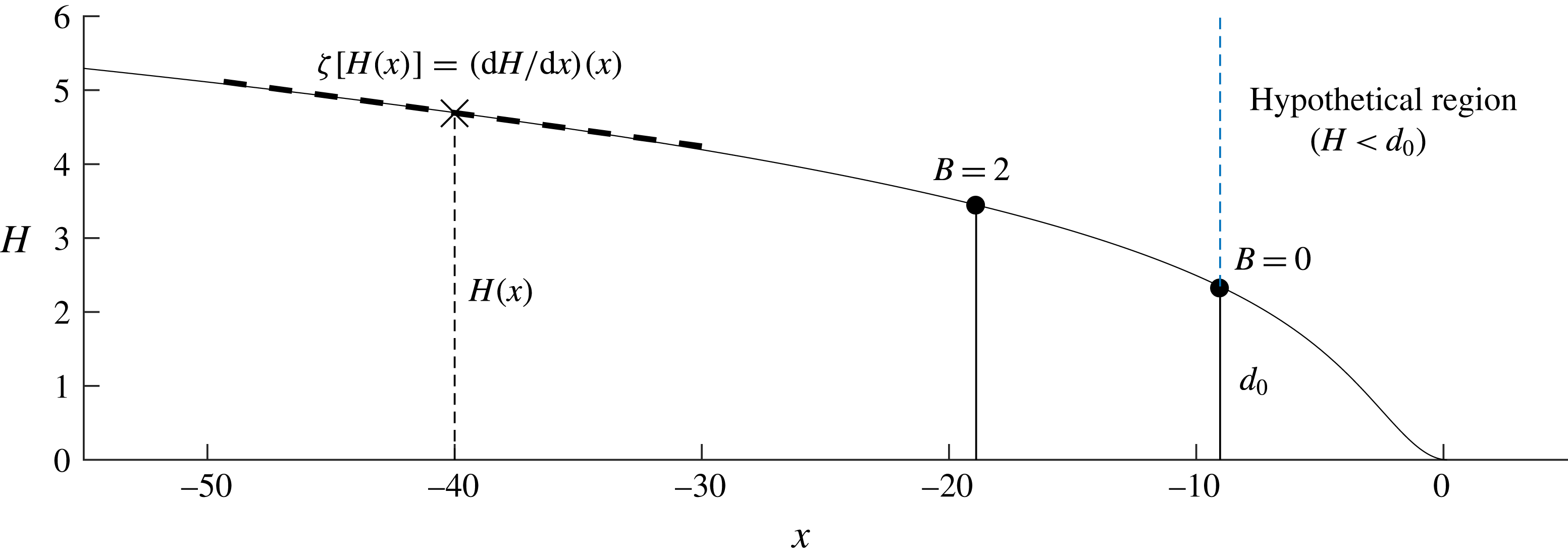
The universal solution describing the thickness profile of the grounded region of the ice sheet. The grounded region of a marine ice sheet will be described by this solution subject to horizontal translation and truncation at a certain thickness controlled by the buttressing force. The leading-order solution for
 $n=1$
and shallow bed slopes
 $|b^{\prime }|\ll 1$
is illustrated here. It is obtained by solving (3.1) numerically by marching forwards until
 $H=0$
, a location set here as the reference position
 $x=0$
. The minimum thickness of truncation in the unbuttressed case occurs at thickness
 $d_{0}\approx 2.345$
, which is illustrated by a vertical dashed line (the region to right of this line is therefore impossible to arise in steady states). The truncating position for a buttressing force
 $B=2$
is also illustrated, corresponding to the case of figure 6. The solution is used to determine the general relationship between the thickness and the thickness gradient,
 $\unicode[STIX]{x1D701}[H(x)]=\text{d}H/\text{d}x(x)$
, of a steady grounded region, and, in turn, the extensional-resistance function (4.3).
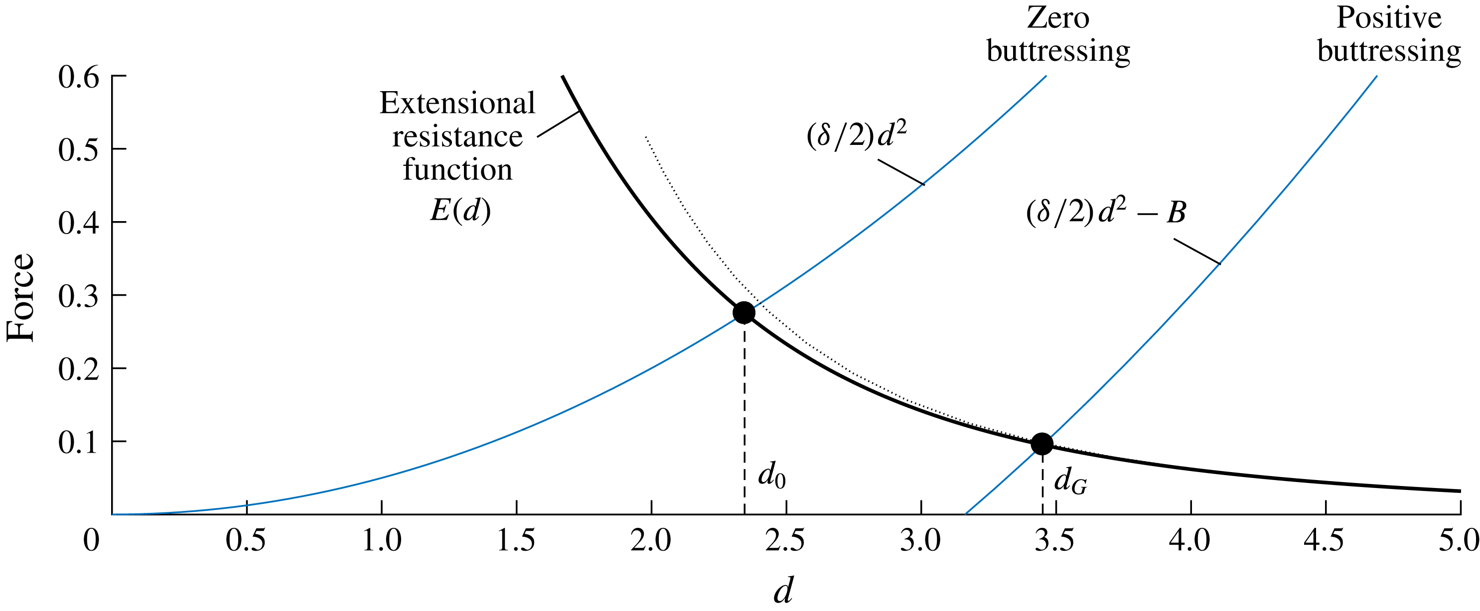
The extensional-resistance function
 $E(d)$
as a function of grounding-line thickness
 $d$
for
 $n=1$
, as calculated in § 4.1 (the solid black curve). Its analytical approximation (4.9) is shown as a dotted black curve. Its intersection with
 $(\unicode[STIX]{x1D6FF}/2)d^{2}-B$
yields the unbuttressed steady-state grounding-line thickness
 $d_{G}=d_{0}\approx 2.345$
for
 $B=0$
and the larger balancing value
 $d_{G}\approx 3.45>d_{0}$
for
 $B=2$
.
With
 $E(d)$
determined, one can explore the predictions of the grounding-line balance (4.2) for different levels of buttressing
 $B$
. For zero buttressing,
 $B=0$
, equation (4.2) simplifies to
 $$\begin{eqnarray}E(d)={\textstyle \frac{1}{2}}\unicode[STIX]{x1D6FF}d^{2}.\end{eqnarray}$$
In this special situation, all the steady-state grounding-line forces depend purely on the grounding-line thickness
 $d$
. Therefore, there is a special balancing value of
 $d$
given by the solution of the algebraic equation (4.4). The individual variations of the sides of the balance as functions of
 $d$
are shown in figure 6, where
 $(\unicode[STIX]{x1D6FF}/2)d^{2}$
is shown as a blue curve and
 $E(d)$
as a black curve. Their intersection yields the critical balancing value
 $d_{G}=d_{0}\approx 2.345$
for
 $n=1$
, which universally describes the steady thickness at an unbuttressed grounding line (for
 $S\ll 1$
and
 $b^{\prime }\ll 1$
). The dimensional expression of this result, namely
 $d/{\mathcal{H}}=d_{0}$
, represents the scaling between grounding-line flux
 $Q$
and thickness
 $d_{G}$
given by Schoof (Reference Schoof2007b
). For the bed profile (2.30), the solution of
 $d(x_{G})=d_{0}$
is given by
 $x_{G}=[\unicode[STIX]{x1D6FD}-(1-\unicode[STIX]{x1D6FF})d_{0}]/\unicode[STIX]{x1D6FC}$
, which is within 1 % of the numerically determined grounding-line position for the examples of figure 4(a,c). The ‘universal profile’ derived above applies for
 $|b^{\prime }|\ll 1$
and
 $S\ll 1$
. The estimates given in § 2.4 indicate that these parameter limits may be broadly relevant to many geophysical settings. Nevertheless, the analysis above can be repeated for
 $\unicode[STIX]{x1D6FC},S\neq 0$
to yield a more general form of the extensional-resistance function
 $E[d(x),\unicode[STIX]{x1D6FC},S]$
that can differ from
 $E[d(x),0,0]$
. For example, the first-order correction to the unbuttressed balance
 $E[d(x),\unicode[STIX]{x1D6FC},0]=(\unicode[STIX]{x1D6FF}/2)d^{2}$
for
 $n=1$
yields
 $d_{G}(\unicode[STIX]{x1D6FC})\sim d_{0}+2.78\,\unicode[STIX]{x1D6FC}$
, for
 $\unicode[STIX]{x1D6FC}\rightarrow 0$
. This represents a correction to the prefactor of the grounding-line flux formula of Schoof (Reference Schoof2007b
) owing to the local basal slope. For
 $|\unicode[STIX]{x1D6FC}|=|b^{\prime }|\lesssim 10^{-2}$
, the case
 $E[d(x),0,0]$
shown in figure 6 provides an excellent approximation.
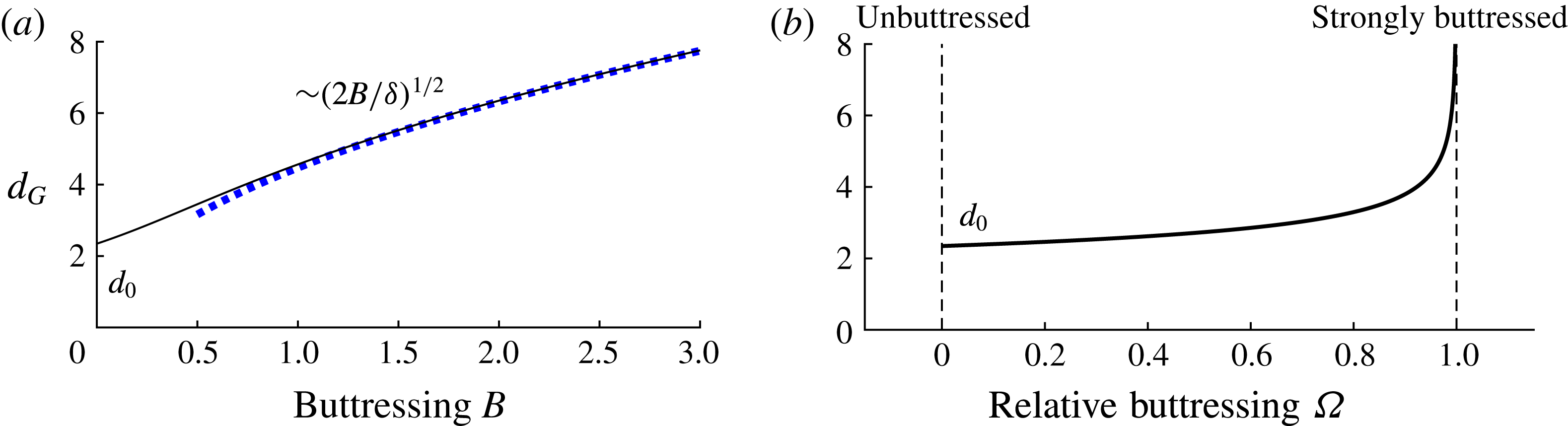
Panel (a) shows the general relationship for
 $n=1$
between the balancing steady-state grounding-line thickness
 $d_{G}$
and the applied buttressing force
 $B$
, as described by the algebraic equation (4.5a
) in which the extensional-resistance function
 $E(d)$
is represented using its numerical solution obtained in § 4.1. The plot shows the increase of the grounding-line thickness
 $d_{G}$
from the special unbuttressed thickness
 $d_{0}$
given by the solution of (4.4). The simplified relationship implied by the strong-buttressing limit of (4.6) is shown as a dashed blue curve. Panel (b) shows the corresponding relationship between the relative buttressing
 $\unicode[STIX]{x1D6FA}$
defined by (4.5b
) and
 $d_{G}$
.
We can deduce some essential effects of ice-shelf buttressing by considering the function
 $E(d)$
in conjunction with the steady-state grounding-line balance equation (4.2) with (for now) a specified buttressing force
 $B$
,
 $$\begin{eqnarray}\displaystyle E(d)+B={\textstyle \frac{1}{2}}\unicode[STIX]{x1D6FF}d^{2}\quad \text{or}\quad \frac{E(d)}{{\textstyle \frac{1}{2}}\unicode[STIX]{x1D6FF}d^{2}}+\underbrace{\frac{B}{{\textstyle \frac{1}{2}}\unicode[STIX]{x1D6FF}d^{2}}}_{\unicode[STIX]{x1D6FA}}=1, & & \displaystyle\end{eqnarray}$$
where
 $\unicode[STIX]{x1D6FA}$
is referred to as the relative buttressing. Application of a numerical root finder to (4.5a
) yields the general relationship between the grounding-line thickness
 $d_{G}$
and the buttressing force
 $B$
for
 $n=1$
shown as a solid curve in figure 7(a). The plot illustrates the increase of the grounding-line thickness
 $d_{G}$
from the unbuttressed value
 $d_{0}$
as the buttressing force
 $B$
is increased.
For sufficiently strong buttressing, equation (4.5a ) predicts a dominant grounding-line balance between the buttressing force and buoyancy alone, namely,
 $$\begin{eqnarray}B\approx {\textstyle \frac{1}{2}}\unicode[STIX]{x1D6FF}d^{2}.\end{eqnarray}$$
This balance represents the strong-buttressing control of a grounding line underlying the reduced nonlinear diffusive flow-line model of Pegler et al. (Reference Pegler, Kowal, Hasenclever and Worster2013). This balance represents a fundamentally different mode of grounding-line control compared to the unbuttressed balance (4.4). A simplified interpretation of the nature of this control as stemming directly from the structure of the ice shelf will be reserved for § 4.3. It follows that there is a complete transition from the ice shelf playing no role whatsoever for a one-dimensional marine ice sheet to playing a potentially completely dominant role for two-dimensional dynamics.
A key question for marine ice sheet dynamics is the proportion of the driving buoyancy drop
 $(\unicode[STIX]{x1D6FF}/2)d^{2}$
that is balanced by buttressing, as measured by
 $\unicode[STIX]{x1D6FA}$
. The general relationship between
 $\unicode[STIX]{x1D6FA}$
and
 $d_{G}$
, as derived from the relationship between
 $B$
and
 $d_{G}$
determined numerically above, is plotted in figure 7(b). The parameter
 $\unicode[STIX]{x1D6FA}$
describes a spectrum of balances bridging two limits: weak buttressing,
 $\unicode[STIX]{x1D6FA}\approx 0$
to strong buttressing
 $\unicode[STIX]{x1D6FA}\approx 1$
. It is related to a quantity
 $\unicode[STIX]{x1D6E9}\equiv (1-\unicode[STIX]{x1D6FA})$
used in the literature to impose a buttressing force as a multiplicative reduction of the driving buoyancy force [
 $E(d)=(\unicode[STIX]{x1D6E9}\unicode[STIX]{x1D6FF}/2)d^{2}$
] (e.g. Dupont & Alley Reference Dupont and Alley2005). The relationship of figure 7(b) gives a prediction for
 $\unicode[STIX]{x1D6FA}$
in terms of the dimensionless grounding-line thickness
 $d_{G}$
. In this case, for
 ${>}$
90 % of the resistance to flow across the grounding line to stem from extension,
 $d_{G}$
must lie in the narrow range
 $d_{0}=2.35<d_{G}<2.40$
. For
 ${>}$
90 % to stem from buttressing,
 $d_{G}>3.8$
.
4.1.1 The force-balance structure
Let the four forces comprising the governing force-balance equation be denoted according to
 $$\begin{eqnarray}\underbrace{4(H\unicode[STIX]{x1D707}u_{x})_{x}}_{E_{x}}-H\unicode[STIX]{x1D70F}_{s}-\unicode[STIX]{x1D70F}_{b}=\underbrace{Hh_{x}}_{G_{x}}.\end{eqnarray}$$
This section will focus on discussing the force balance specifically in the grounded region and hence
 $\unicode[STIX]{x1D70F}_{s}$
will be set as zero for the time being (its effects on force-balance structure are reserved for § 5). The three remaining forces are plotted for the final steady state for the unbuttressed example (
 $\unicode[STIX]{x1D70F}_{s}\equiv 0$
) shown earlier in figure 4(a). Here, the divergence of the depth-integrated extensional stress
 $E_{x}$
is shown as a solid curve, the basal stress
 $\unicode[STIX]{x1D70F}_{b}$
is shown as a dashed curve and the gravitational term
 $G_{x}$
as a dotted curve. Upstream, the divergence of extensional stresses
 $E_{x}$
is small and hence the flow is dominated by a balance between the total drag and gravity,
 $\unicode[STIX]{x1D70F}_{b}\sim G_{x}$
, for which (2.24a
) reduces to the simplified flow equation
 $$\begin{eqnarray}\unicode[STIX]{x1D70F}_{b}\approx -H\frac{\unicode[STIX]{x2202}h}{\unicode[STIX]{x2202}x}.\end{eqnarray}$$
This drag-dominated balance is mathematically similar to the balance associated with the shallow-ice-approximation, which refers specifically to a leading-order balance between vertical shear stresses and gravity (Fowler & Larson Reference Fowler and Larson1978; Cuffey & Paterson Reference Cuffey and Paterson2010). Towards the grounding line,
 $E_{x}$
increases very slightly, but remains small. Therefore the approximation of (4.8) holds all the way up to and including the grounding line. Across the grounding line, basal stress vanishes abruptly,
 $\unicode[STIX]{x1D70F}_{b}\equiv 0$
and
 $E_{x}\equiv G_{x}$
for
 $x>x_{G}$
. The steady-state grounding-line position
 $x_{G}$
is set by where the extensional stress
 $E$
balances the buoyancy force in accordance with (4.4). It is therefore interesting that its divergence
 $E_{x}$
remains uniformly small throughout the grounded region. As a consequence, there is no boundary layer through which the basal-drag-dominated approximation of (4.8) breaks down. The lack of this boundary layer can be attributed to the smallness of the dimensionless density difference
 $\unicode[STIX]{x1D6FF}\approx 0.1$
, which appears as a prefactor to the gravitational term in (2.28) but not in (2.24a
). As a consequence,
 $E_{x}=O(\unicode[STIX]{x1D6FF}E)$
at the location where the grounding-line balance of (2.28) is satisfied, and is therefore small. By rewriting (2.28) as
 $H=8\unicode[STIX]{x1D6FF}^{-1}\unicode[STIX]{x1D707}\unicode[STIX]{x2202}u/\unicode[STIX]{x2202}x$
, it is explicitly seen that (2.28) is attained for a relatively larger thickness
 $H$
as
 $\unicode[STIX]{x1D6FF}\rightarrow 0$
. In other words, the universal profile of the grounded region shown in figure 5 is truncated further upstream for smaller
 $\unicode[STIX]{x1D6FF}$
. The geophysical value of
 $\unicode[STIX]{x1D6FF}=0.1$
is sufficiently small that the grounding line occurs at a thickness where
 $E_{x}$
is still small (the value of
 $E_{x}$
only becomes important in the ‘hypothetical region’ residing to the right of the vertical dashed line in figure 5). The limit of
 $\unicode[STIX]{x1D6FF}\rightarrow 0$
thus represents an asymptotic condition under which the basal-drag-dominated zone can be matched to the extensional ice shelf formally, and to excellent approximation, using a direct patching condition. In this regard, there is no boundary layer through which terms in the governing equation (2.14a
) change their order of magnitude. It should be emphasised that the notion of an extensional boundary layer discussed here is conceptually distinct from the notion of a boundary layer described in § 2.3, which is used only to neglect accumulation near the grounding line.
The profiles of forces comprising the force-balance equation (4.7) along the length of an unbuttressed marine ice sheet,
 $S=0$
. The divergence of extensional stresses
 $E_{x}$
is shown as solid black curve, basal stress
 $\unicode[STIX]{x1D70F}_{b}$
is shown as a dotted blue curve and gravity
 $G_{x}$
is shown as a dashed black curve. Panel (a) illustrates the satisfaction of the basal-drag-dominated balance (
 $\unicode[STIX]{x1D70F}_{b}\approx G_{x}$
) given by (4.8) for
 $x<x_{G}$
. The enlargement of (b) shows the jump to an extension-dominated ice shelf (
 $E_{x}\equiv G_{x}$
).
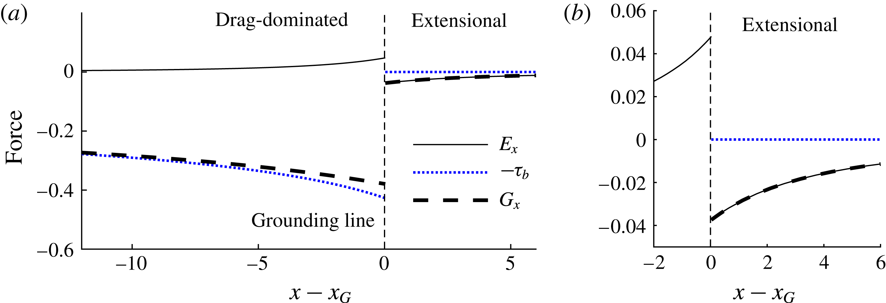
It will be verified later in § 5.1 that the force balance throughout the grounded region is qualitatively similar with buttressing. Indeed, buttressing strengthens the drag-dominated approximation (4.8) even more because it causes the universal profile to be truncated at a yet thicker grounding line
 $d_{G}>d_{0}$
, as illustrated for
 $B=2$
in figure 5. However, lateral stresses fundamentally complicate the force-balance structure of the ice shelf (Pegler Reference Pegler2016), an aspect reserved for § 5.
4.1.2 Analytical approximation for
$E$

By using (4.8) to evaluate the thickness-gradient function
 $\unicode[STIX]{x1D701}(H)$
in (4.3), one obtains the analytical approximation for the extensional-resistance function
 $$\begin{eqnarray}E(d)\approx 4d^{-3},\end{eqnarray}$$
given here for
 $n=1$
. This approximation is plotted alongside the numerical solution in figure 6 as a dotted curve. The generalisation of this result to other values of
 $n$
, and an effect of local slope
 $b^{\prime }$
, is obtained in appendix A. The approximation provides an excellent representation of the numerically determined curve. To illustrate its accuracy, note that a substitution of (4.9) into (4.4) and rearrangement for
 $d_{0}$
yields
 $d_{0}\approx (8/\unicode[STIX]{x1D6FF})^{1/5}$
, which is within 15 % of the exact value. The corresponding result for
 $n=3$
is within a mere 0.1 % of the exact result (see appendix A). Thus, the neglect of the divergence of extensional stresses, which is responsible for long-range communication of forces in the grounded region of an ice sheet, has practically no effect on the predictions of the SSA model (at least for steady or near-steady grounding-line balances).
4.2 The buttressing resistance function
$B$

This section determines the steady-state buttressing force
 $B$
in terms of the parameters specifying the ice-shelf dynamics. In steady state, the integral form of the buttressing force defined in (4.1) is given by
 $$\begin{eqnarray}B[x_{G},x_{C},d_{G}]=\int _{x_{G}}^{x_{C}}H\unicode[STIX]{x1D70F}_{s}(u)\,\text{d}x=S\int _{x_{G}}^{x_{C}}Hu^{m}\,\text{d}x,\end{eqnarray}$$
where
 $u(x)$
is the solution to the steady-state system describing the ice shelf (3.1b
) integrated subject to a ‘prescribed’ grounding-line thickness
 $d_{G}$
and the frontal stress condition (3.2a
), namely,
 $$\begin{eqnarray}\displaystyle u(x_{G})=d_{G}^{-1},\quad u^{\prime }(x_{C})=[\unicode[STIX]{x1D6FF}/8u(x_{C})]^{1/m}. & & \displaystyle\end{eqnarray}$$
The system defined by (3.1) and (4.11a,b
) depends on
 $x_{G}$
,
 $x_{C}$
and
 $d_{G}$
, and hence the steady-state buttressing force (4.10) is a function of these variables alone. The function
 $B[x_{G},x_{C},d_{G}]$
can be interpreted as a ‘database’ giving the steady-state buttressing force for any given
 $x_{G}$
,
 $x_{C}$
and
 $d_{G}$
. A similar method of constructing database functions for steady-state buttressing forces was developed for a radially spreading ice shelf (Pegler & Worster Reference Pegler and Worster2012, Reference Pegler and Worster2013), for which a reduction to an algebraic system analogous to (4.2) was obtained.
The translational invariance of the system defined by (3.1) and (4.11a,b
) implies that the dependences of
 $B$
on
 $x_{G}$
and
 $x_{C}$
can be combined into a single dependence on shelf length,
 $L\equiv x_{C}-x_{G}$
. Integrating (3.1b
) subject to (4.11a,b
) numerically using a scheme similar to that described earlier in the text below (3.1) and evaluating the integral of (4.10) using quadrature over a range of
 $L$
, I determine the general relationship between
 $B$
and shelf length
 $L$
for two illustrative fixed values of
 $d_{G}=4$
and 16 in figure 9. The numerical similarity of the two curves indicates a very weak dependence of buttressing on grounding-line thickness
 $d_{G}$
. In other words, for each value of
 $n$
, there is a near-universal relationship between buttressing and shelf length spanning fully the limit of a short, weakly buttressing ice shelf to a long, strongly buttressing ice shelf.
The relationship between the buttressing force (4.10) and shelf length
 $L\equiv x_{C}-x_{G}$
for grounding-line thicknesses of
 $d_{G}=4$
(solid) and 16 (dashed) and power-law exponent
 $n=3$
obtained by repeatedly solving (3.1) and (4.11) numerically and evaluating the integral in (4.10) using quadrature. The analytical approximation (4.13) is shown as a dotted blue curve, illustrating its excellent representation of the buttressing force.
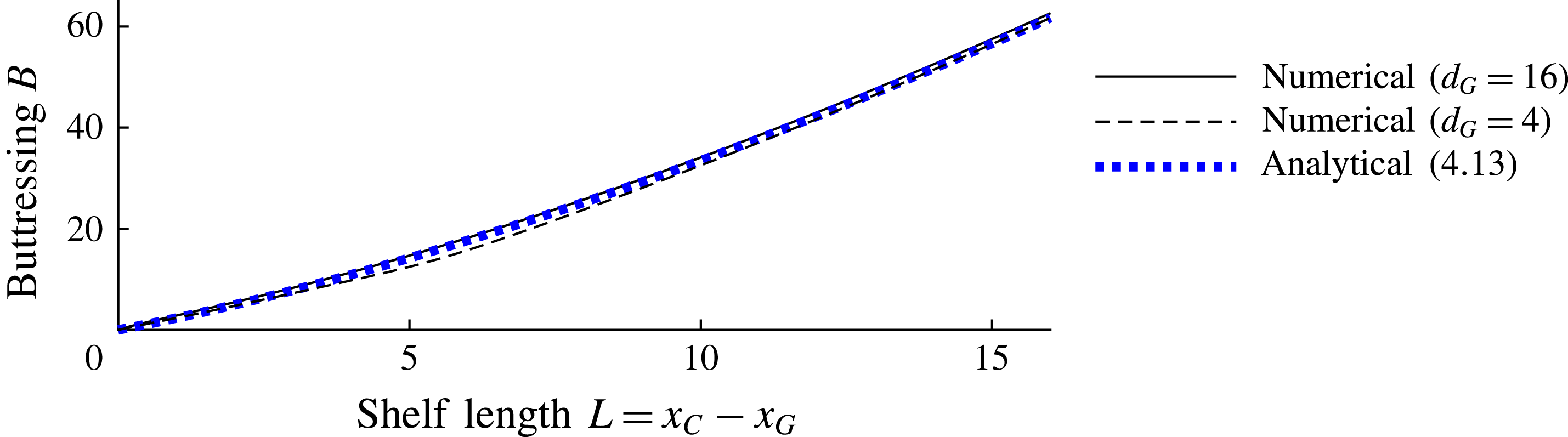
For
 $n=1$
, equation (4.10) can be integrated directly to give (Pegler Reference Pegler2016)
 $$\begin{eqnarray}B=S(x_{C}-x_{G}),\end{eqnarray}$$
showing that, for linear rheology, the buttressing force is directly proportional to the length of the ice shelf. The possibility of this simple integration applies uniquely for
 $n=1$
because the integrand of (4.10) is uniformly proportional to the width-averaged flux
 $Hu=1$
. Expression (4.12) implies that there is no dependence of the steady-state buttressing force for
 $n=1$
on the grounding-line thickness
 $d_{G}$
.
For
 $n>1$
, one can develop the generalised analytical approximation
 $$\begin{eqnarray}B\approx \frac{\unicode[STIX]{x1D6FF}}{2}\left\{\left[\frac{NS}{\unicode[STIX]{x1D6FF}}(x_{C}-x_{G})+H_{C}^{N}\right]^{2/N}-H_{C}^{2}\right\},\end{eqnarray}$$
where
 $N\equiv (n+1)/n$
,
 $H_{C}\approx 8^{1/N^{2}}\unicode[STIX]{x1D702}$
is the calving thickness and
 $\unicode[STIX]{x1D702}\equiv \unicode[STIX]{x1D6FF}^{-1/N}S^{1/nN^{2}}$
. This excellent approximation follows from substitution of the analytical solution for the prevailing interior of the ice shelf derived in Pegler (Reference Pegler2016) into the buttressing integral (4.10), as detailed in appendix A. The result of (4.13) is shown as a dotted blue curve in figure 9 and closely approximates the two numerical curves. The lack of a dependence of (4.13) on
 $d_{G}$
corroborates the very weak dependence of the numerical solutions on
 $d_{G}$
. The weak dependence occurs because
 $d_{G}$
only affects flow in the transitional boundary layer in front of the grounding line, which provides a relatively small contribution to the buttressing integral (4.10). For
 $n>1$
, equation (4.13) shows that a shear-thinning rheology causes
 $B$
to depend nonlinearly on the shelf length
 $(x_{C}-x_{G})$
and introduces a dependence on the calving thickness
 $H_{C}$
(a known quantity that is determined as part of the analytical solution of the universal profile (A 4)).
Panels (a–c) illustrate the profile of the marine ice sheet as the dimensionless lateral-drag coefficient
 $S$
is increased through 0,
 $2\times 10^{-3}$
and
 $10^{-2}$
, respectively, for topography defined by
 $\unicode[STIX]{x1D6FC}=-2\times 10^{-3}$
and
 $\unicode[STIX]{x1D6FD}=2.8$
. The plot illustrates the change in form of the ice sheet from zero buttressing to positive buttressing. Panel (d) shows the corresponding grounding-line position
 $x_{G}$
across this range. The strong-buttressing prediction of (4.6) is shown as a curve of blue circles. Panel (e) shows the corresponding variation of the relative buttressing parameter
 $\unicode[STIX]{x1D6FA}$
defined by (4.5). The threshold (4.15) for large
 $S$
is shown as a horizontal dashed line.
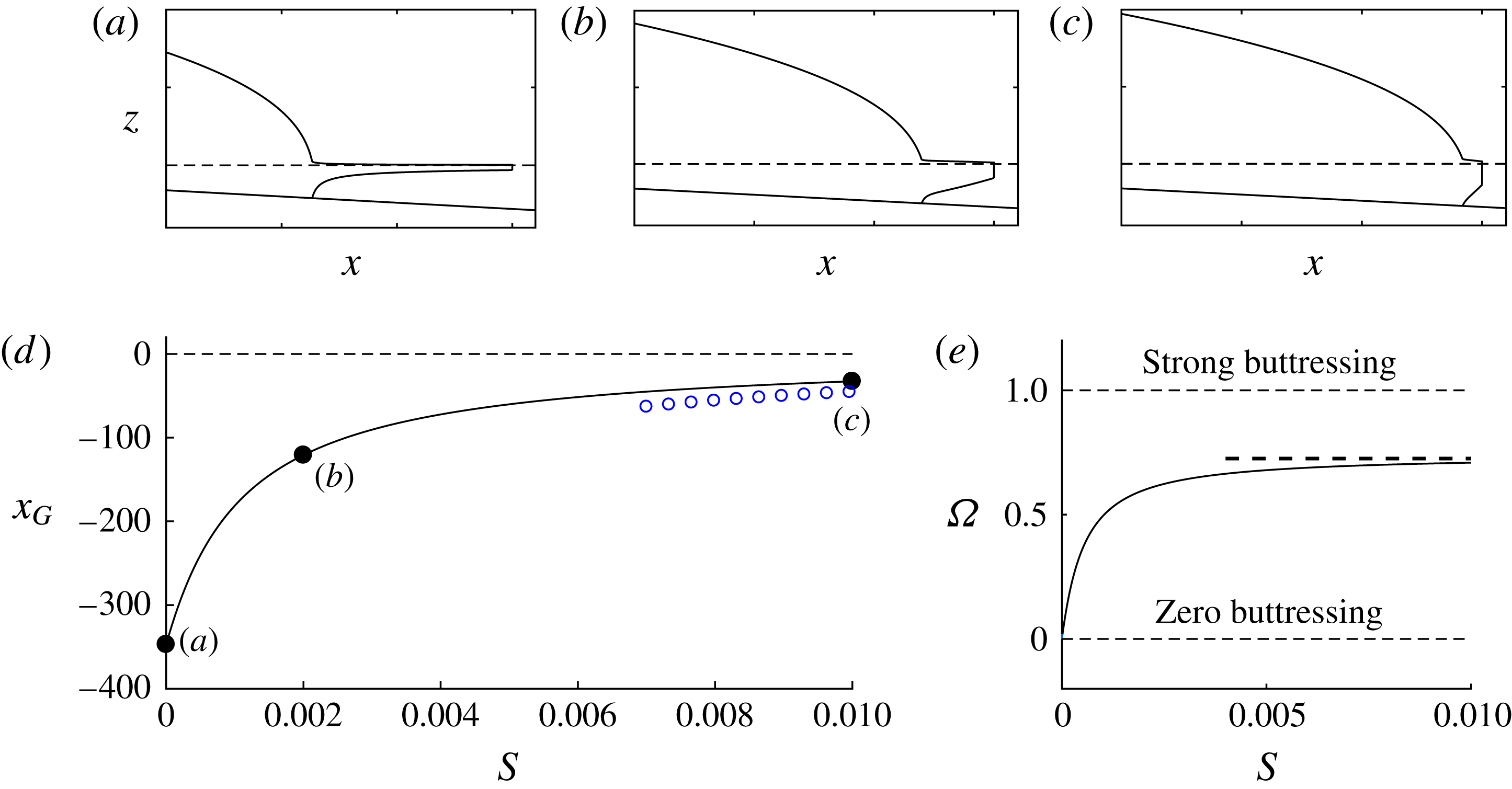
Net accumulation in the ice shelf has a direct dynamical effect via its control of ice-shelf buttressing. By integrating the steady-state form of (2.18), one obtains the non-uniform flux per unit width
 $q(x)=Hu=1+\int _{x_{G}}^{x}F(x^{\prime })\,\text{d}x$
. With this, the generalisation of (4.13), derived in appendix A, is
 $$\begin{eqnarray}B\approx \frac{\unicode[STIX]{x1D6FF}}{2}\left\{\left[\frac{N}{\unicode[STIX]{x1D6FF}}\int _{x_{G}}^{x_{C}}Sq(x^{\prime })^{(1/n)}\,\text{d}x^{\prime }+H_{C}^{N}\right]^{2/N}-H_{C}^{2}\right\},\end{eqnarray}$$
which relates the distribution of melting
 $F(x)$
to the buttressing force. This expression embodies the key link between the oceanographic control of melting (e.g. Jenkins Reference Jenkins1991) and glacial dynamics. The result shows that buttressing generally depends on the integral of the flux along the ice shelf
 $q(x)$
. An interesting implication is that melting near the grounding line, which can be the most significant along the ice shelf, has a larger effect on the buttressing than melting further downstream because of the longer region over which it reduces the flux of the ice shelf.
4.3 Dynamical variation across the spectrum of relative buttressing strength
When the function (4.12) (or one of its generalisations, (4.13) or (4.14)) is incorporated into (4.2) along with
 $E[d(x)]$
, the full equation provides a closed algebraic equation for the position of steady-state grounding lines
 $x_{G}$
. The equation bridges the complete spectrum connecting unbuttressed to strongly buttressed grounding lines. This equation incorporates ice-shelf buttressing predictively, contrasting with a direct prescription of
 $\unicode[STIX]{x1D6E9}$
(e.g. Dupont & Alley Reference Dupont and Alley2005).
To demonstrate the application of the balance equation (4.2), I solve it for
 $x_{G}$
for the illustrative example of the negative slope
 $\unicode[STIX]{x1D6FC}=-2\times 10^{-3}$
and reference ocean depth
 $\unicode[STIX]{x1D6FD}=2.8$
. The predicted grounding-line position
 $x_{G}$
is plotted as a function of the dimensionless lateral-drag coefficient
 $S$
in figure 10(d), showing the positioning of the grounding line in deeper water for larger
 $S$
. Panels (a–c) illustrate the flow profile of a marine ice sheet as
 $S$
is increased, showing the transition from the broadly concave ice-shelf profile of a non-buttressing ice shelf (van der Veen Reference van der Veen1983) to the more wedge-shaped profile of a buttressing ice shelf (Pegler Reference Pegler2016). The corresponding relative buttressing
 $\unicode[STIX]{x1D6FA}$
is shown in figure 10(b). The plot shows a sharp increase in the relative buttressing with
 $S$
towards the regime of strong buttressing. As
 $S$
is increased,
 $\unicode[STIX]{x1D6FA}$
asymptotes towards the value 0.7 shown as a horizontal dashed line. Perhaps surprisingly, this value is less than unity. This upper bound on the relative buttressing arises because the buttressing cannot balance the hydrostatic pressure drop between the calving front and the ocean immediately in front of it. This property will be discussed further in the text below (5.4). The asymptotic value of
 $\unicode[STIX]{x1D6FA}$
is obtained by substituting the flotation depth of the ocean at the calving front,
 $d_{C}\equiv \unicode[STIX]{x1D6FD}/(1-\unicode[STIX]{x1D6FF})$
, into (4.5b
) to determine that
 $$\begin{eqnarray}\unicode[STIX]{x1D6FA}\leqslant \unicode[STIX]{x1D6FA}_{C}=1-\frac{E(d_{C})}{{\textstyle \frac{1}{2}}\unicode[STIX]{x1D6FF}d_{C}^{2}}.\end{eqnarray}$$
For
 $\unicode[STIX]{x1D6FD}=2.8$
,
 $\unicode[STIX]{x1D6FA}_{C}\approx 0.7$
, in agreement with the asymptotic behaviour of
 $\unicode[STIX]{x1D6FA}$
determined numerically. The large-
 $S$
solution can be approximated by the strong-buttressing limiting balance of (4.6), which is shown as a curve of blue circles in figure 10(d).
As
 $S$
is increased, there is a fundamental switch in the dominant forces controlling the grounding line. To illustrate this, I express the limiting end-member balances predicted by (4.2) in their dimensional forms. For
 $n=1$
, these are given by
 $$\begin{eqnarray}\displaystyle \left.\begin{array}{@{}c@{}}E(d)=\displaystyle \frac{4\unicode[STIX]{x1D707}_{0}Q^{2}C_{-}}{\unicode[STIX]{x1D70C}gd(x)^{3}}\sim \displaystyle \frac{\unicode[STIX]{x1D70C}g^{\prime }d(x)^{2}}{2}\quad (\unicode[STIX]{x1D6FA}=0),\\ B(x_{C}-x_{G})=\displaystyle \frac{3\unicode[STIX]{x1D707}_{0}Q}{w^{2}}(x_{C}-x_{G})\sim \displaystyle \frac{\unicode[STIX]{x1D70C}g^{\prime }d(x)^{2}}{2}\quad (\unicode[STIX]{x1D6FA}\approx 1).\end{array}\right\} & & \displaystyle\end{eqnarray}$$
The extension-dominated unbuttressed balance of (4.16a
) recovers the expression for
 $Q$
as a function of grounding-line thickness
 $d$
given by Schoof (Reference Schoof2007b
). This first result shows that an unbuttressed grounding-line position is influenced by the viscosity of the ice
 $\unicode[STIX]{x1D707}_{0}$
and the basal-drag coefficient
 $C_{-}$
. In this case, the balance can be interpreted as an expression for the grounding-line thickness, as represented by the special dimensionless thickness
 $d_{0}$
discussed above. The pure dependence of (4.16a
) on the single dependent variable
 $d(x)$
is consistent with the simplified situation of an unbuttressed grounding being controlled directly by the local grounding-line thickness. The strong-buttressing expression of (4.16b
) represents a completely different physical control of the grounding-line position dominated instead by the ice-shelf dynamics. This includes an inherent dependence on the calving position
 $x_{C}$
and width of the ice shelf
 $w$
, and a loss of dependence on the basal drag coefficient
 $C_{-}$
. Thus, there is a full switch in dynamical control from the calving position playing no role whatsoever for a one-dimensional or non-buttressing marine ice sheet to playing a dominant control under the effect of even relatively weak lateral stresses on the ice shelf.
It should be noted that the application of the augmented expression for grounding-line flux in a form that incorporates the multiplicative reduction in the hydrostatic-pressure drop owing to buttressing
 $\unicode[STIX]{x1D6E9}$
(Schoof Reference Schoof2007b
), and used in simulations (e.g. DeConto & Pollard Reference DeConto and Pollard2016), becomes degenerate for sufficiently strong buttressing. The general balance equation in the form (4.2) will seamlessly incorporate both unbuttressed and strongly buttressed situations.
Suites of steady-state profiles of a marine ice sheet for (a) zero lateral stress,
 $S=0$
, and (b) a positive lateral stress,
 $S=2\times 10^{-3}$
shown as the calving position
 $x_{C}$
is varied. The plot illustrates the complete independence of the grounding line from the calving position
 $x_{C}$
for case (a) and the considerable sensitivity to it in case (b). Overlaid as a red dotted curve in (b) is a solution with the same parameters as the case
 $x_{C}=400$
but with the basal stress set identically equal to zero to leave just the lateral drag, illustrating the effective independence of the grounding line from the nature of the drag force in the grounded region.
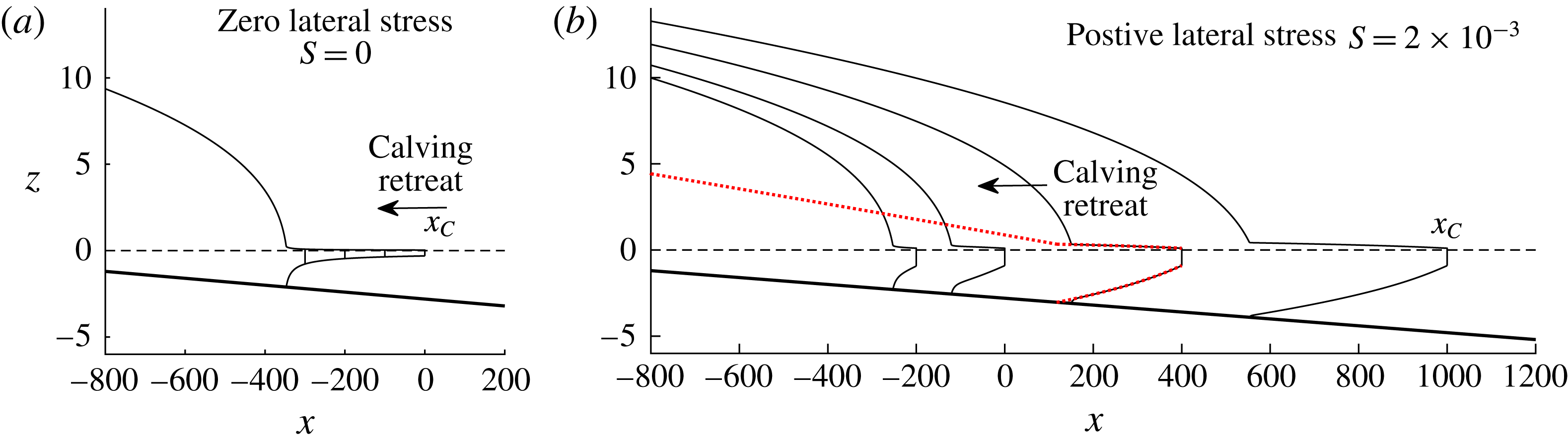
The key switch in parametric dependence from the ice shelf playing a non-existent role to a dominant role is illustrated explicitly by the variation of the steady-state solutions for a selection of calving positions
 $x_{C}$
shown in figure 11 for (a)
 $S=0$
and (b)
 $S=2\times 10^{-3}$
. For the unbuttressed case (a), there is no change in the grounding-line position
 $x_{G}$
. In the buttressing case (b), a considerable change in grounding-line position occurs. As the calving position is varied, the change in grounding-line position is in fact larger than the change in the ice-shelf length. In this same plot, I illustrate as a red dotted curve a solution in which the basal stress, given by the third term in (3.1a
) is set identically equal to zero for the case
 $x_{C}=400$
. The grounding-line position is essentially unaffected despite the complete removal of basal stress. The grounding line is therefore being controlled completely by the ice shelf.
5 Marine ice sheet structure
Analysis of the solutions of the floating component of the Q2D model (Pegler Reference Pegler2016) shows that the form of a buttressing ice shelf differs from the broad concave profile of a non-buttressing ice shelf (e.g. van der Veen Reference van der Veen1983) in containing a short region of rapid thinning in front of the grounding line connected to a prevailing region of relatively mild slope leading to the calving front. This section will review this structure and draw connections between certain variables defining the structure of an ice shelf and the relative strength of buttressing that it generates.
5.1 Effect of lateral stresses on the structure of the ice sheet
To illustrate the force-balance structure with lateral stresses, I show the profiles of the four individual forces comprising the continuum balance (4.7) for the illustrative case of
 $S=2\times 10^{-3}$
in figure 12, where the lateral stress
 $\unicode[STIX]{x1D70F}_{s}$
is indicated by a red dashed curve, which is horizontal for
 $x>x_{G}$
. In common with the unbuttressed case shown earlier in figure 8, the grounded region is basal-drag-dominated, with the divergence of extensional stress
 $E_{x}$
being negligible along its full length. However, the ice shelf forms two distinct regions: the ‘input boundary layer’ in which extensional stresses are important and the prevailing ‘universal profile’ of the ice shelf further downstream (Pegler Reference Pegler2016) in which the transverse shear stresses provide the dominant resistance to flow.
Panel (a) shows the numerical solution for
 $\unicode[STIX]{x1D6FD}=2.8$
,
 $\unicode[STIX]{x1D6FC}=2\times 10^{-3}$
and
 $S=2\times 10^{-3}$
, and illustrates the three-component structure of a buttressed marine ice sheet. The profiles of forces, as defined in (4.7), are shown in (b). Here, the divergence of extensional stresses
 $E_{x}$
is shown as solid black curve, basal stress
 $\unicode[STIX]{x1D70F}_{b}$
is shown as a dotted blue curve, the dimensionless depth-integrated lateral stress
 $H\unicode[STIX]{x1D70F}_{s}$
is shown as a dotted red curve and the gravitational force
 $G_{x}$
is shown as a dashed black curve. The plots illustrate the basal-drag-dominated grounded balance (
 $\unicode[STIX]{x1D70F}_{b}\approx G_{x}$
), the extensional inlet boundary layer in front of the grounding line,
 $x_{G}<x<x_{G}+\unicode[STIX]{x1D6E5}$
, and the lateral-drag-dominated region downstream (
 $H\unicode[STIX]{x1D70F}_{s}\approx G_{x}$
). The enlargement given in (c) shows the extensional balance (
 $E_{x}\approx G_{x}$
) in the inlet boundary layer.
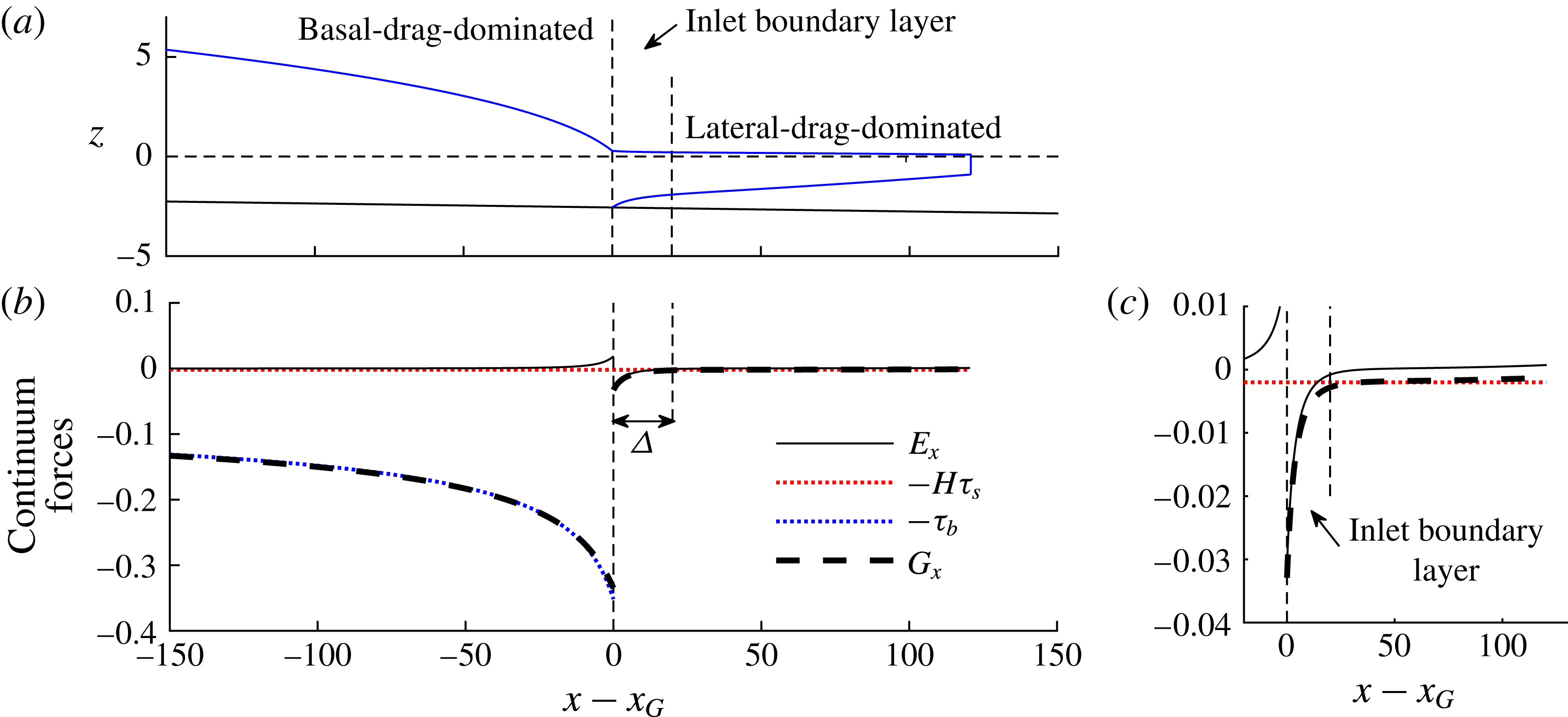
To analyse this asymptotic structure, I first recall the general analytical solution describing the confined ice shelf for
 $n=1$
given by solving (3.1) subject to (4.11a,b
), namely,
 $$\begin{eqnarray}H(x)=\unicode[STIX]{x1D702}\left[\text{e}^{\tilde{x}^{2}/4}\left(\tilde{d}_{G}^{-2}\text{e}^{-\tilde{x}_{G}/4}+\frac{1}{2}\int _{-\tilde{x}/2}^{-\tilde{x}_{G}/2}\text{e}^{-\unicode[STIX]{x1D709}^{2}}\,\text{d}\unicode[STIX]{x1D709}\right)\right]^{-1/2},\end{eqnarray}$$
where
 $\unicode[STIX]{x1D702}\equiv (S/\unicode[STIX]{x1D6FF}^{2})^{1/4}$
,
 $(\tilde{x},\tilde{x}_{G})\equiv S^{1/2}(x,x_{G})$
,
 $\tilde{d}_{G}\equiv \unicode[STIX]{x1D702}^{-1}d_{G}$
(Pegler Reference Pegler2016). The solution (5.1) is illustrated for two shelf lengths
 $L=100$
and 500 in figure 13(b,c). The solution for
 $L=100$
clearly illustrates the inlet boundary layer of rapid thinning. The prevailing downstream region is independent of the grounding-line thickness
 $d_{G}$
and dominantly controlled by the calving position
 $x_{C}$
. By considering the asymptotic structure of (5.1), one can determine the solution for the prevailing downstream region,
 $$\begin{eqnarray}H_{U}(x)=\unicode[STIX]{x1D702}\left[{\textstyle \frac{1}{4}}\sqrt{\unicode[STIX]{x03C0}}\,\text{erfcx}\,(-{\textstyle \frac{1}{2}}\tilde{x})\right]^{-1/2}\quad (\unicode[STIX]{x1D6E5}\lesssim x\leqslant x_{C}),\end{eqnarray}$$
where
 $\text{erfcx}\,\unicode[STIX]{x1D701}\equiv \text{e}^{\unicode[STIX]{x1D701}^{2}}(1-\text{erf}\,\unicode[STIX]{x1D701})$
and
 $\unicode[STIX]{x1D6E5}$
is the length of the inlet boundary layer, which varies depending on the solution (Pegler Reference Pegler2016). The downstream solution (5.2) is shown as a dashed blue curve in figure 13(b,c) and is confirmed to describe the prevailing shape. The corresponding analytical result for power-law fluid (Pegler Reference Pegler2016) is reviewed in appendix A. If the ‘matching thickness’ of the universal profile (5.2) extrapolated to the grounding line, namely
 $H_{+}\equiv H_{U}(x_{G})$
, is less than the grounding-line thickness,
 $H_{+}<d_{G}$
, then the flow through the inlet boundary layer is characterised by thinning and acceleration. This situation, referred to as ‘over-thick’, corresponds to the profile of an ice shelf typically observed in nature. On this basis, it was hypothesised in Pegler (Reference Pegler2016) that the predictions of a full marine ice sheet model for steady-state balances should only produce this situation. If instead,
 $H_{+}>d_{G}$
, then the inlet involves thickening and deceleration, and was referred to as ‘under-thick’. An under-thick input is a theoretical possibility only if one has full control over the specification of the inlet thickness and position, and may never arise in the glaciological context. However, for input configurations involving the direct input at an imposed position or along a back wall, an under-thick flow is possible; this situation was observed in the laboratory experiments of Pegler (Reference Pegler2016) and may occur in float-glass manufacture.
Panel (a) shows the steady-state grounding-line thickness
 $d_{G}$
as a function of the shelf length
 $L=x_{C}-x_{G}$
for
 $S=2\times 10^{-3}$
, compared alongside the value of the universal profile (5.2) extrapolated to the input
 $H_{+}\equiv H_{U}(x_{G})$
. It is found that
 $d_{G}>H_{+}$
, implying that only over-thick regimes of input occur for marine ice sheets. The vertical dashed line indicates the characteristic length
 $2S^{-1/2}\approx 44$
above which the distinction between the universal profile and the inlet boundary layer is clearly developed. The inset shows the relative buttressing parameter
 $\unicode[STIX]{x1D6FA}$
defined by (4.5) plotted as a function of shelf length and the associated approximation based on (5.4). Panels (b,c) show the analytical solution (5.1) (solid black curve) and the universal profile (5.2) (dashed, blue curves) for
 $L=100$
and 500, respectively.
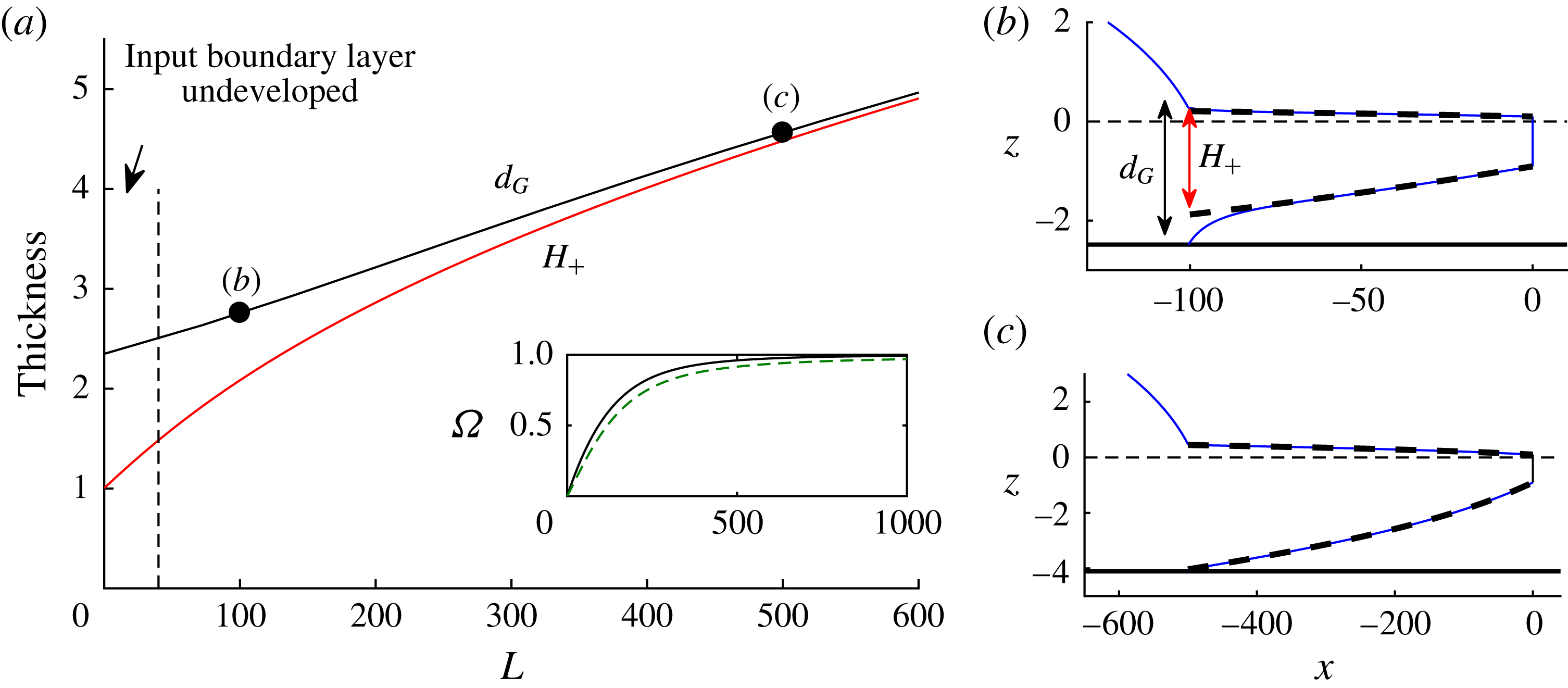
To illustrate the variation in the ice-shelf structure as the shelf length
 $L$
is increased from zero, I show the grounding-line thickness
 $d_{G}$
predicted by the grounding-line balance equation (4.2) alongside the matching thickness
 $H_{+}$
predicted by (5.2) against
 $L$
for
 $S=2\times 10^{-3}$
in figure 13(a). The results show that
 $d_{G}>H_{+}$
, confirming the hypothesis that only over-thick input boundary layers can arise in the glacial context (at least in steady state). It should be noted that the inlet boundary layer is clearly defined only for a sufficiently long ice shelf,
 $L\gtrsim S^{-1/2}\hat{L}\approx 44$
, a value indicated by the vertical dashed line in figure 13(a) (this corresponds to the length of the ice shelf being greater than approximately one third of its width). For sufficiently large
 $L$
, figure 13(a) shows that the extrapolated and grounding-line thicknesses become similar,
 $H_{+}\approx d_{G}$
. The grounding line then occurs to excellent approximation where (5.2) intersects the bedrock, as illustrated in figure 13(c), implying that the grounding line is being controlled independently by the lateral-drag-dominated section of the ice shelf (cf. Pegler et al.
Reference Pegler, Kowal, Hasenclever and Worster2013).
5.2 Relationship between the buttressing force and the structure of the ice shelf
Analogously to the simplifications arising from the basal-drag-dominated approximation in the grounded region (4.8), analytical results can be determined using the uniform smallness of
 $E_{x}$
throughout the component of the ice shelf downstream of the inlet boundary layer. Similarly to that case, the divergence of extensional stresses
 $E_{x}$
remains small throughout the flow downstream of the input boundary layer, as shown in figure 12. It was noted in § 4.1.2 that this could be justified on the basis of the smallness of
 $\unicode[STIX]{x1D6FF}$
. However, in the purely floating context there is no parameter limit analogous to
 $\unicode[STIX]{x1D6FF}\rightarrow 0$
to justify the uniform smallness of
 $E_{x}$
. Despite this, the numerical value of
 $E_{x}\approx 10^{-2}E$
at
 $x=x_{C}$
for
 $n=3$
, is verifiably small (in a sense, ‘
 $\unicode[STIX]{x1D6FF}=1$
’ is small enough). Thus, the analytical approximations for the universal profiles resulting from the neglect of
 $E_{x}$
, as derived in Pegler (Reference Pegler2016) and reviewed by (A 4) in appendix A, provide practically exact descriptions of the prevailing region of the ice shelf downstream of the inlet boundary layer (there is a maximum error of just 2 %).
The neglect of
 $E_{x}$
in (2.24b
) yields the lateral-drag-dominated flow approximation
 $$\begin{eqnarray}\unicode[STIX]{x1D70F}_{s}\approx -\unicode[STIX]{x1D6FF}H^{\prime },\end{eqnarray}$$
which is the floating analogue of (4.8). Since this approximation applies uniformly downstream of the inlet boundary layer (Pegler Reference Pegler2016), one can evaluate (4.13) as
 $$\begin{eqnarray}B\approx \int _{x_{G}+\unicode[STIX]{x1D6E5}}^{x_{C}}H\unicode[STIX]{x1D70F}_{s}\,\text{d}x\approx \left[-\frac{1}{2}\unicode[STIX]{x1D6FF}H^{2}\right]_{x_{G}+\unicode[STIX]{x1D6E5}}^{x_{C}}\approx \frac{1}{2}\unicode[STIX]{x1D6FF}[H_{U}(x_{G})]^{2}-\frac{1}{2}\unicode[STIX]{x1D6FF}H_{C}^{2}\end{eqnarray}$$
on neglecting the contribution over
 $[x_{G},x_{G}+\unicode[STIX]{x1D6E5}]$
. The result of (5.4) shows that the buttressing force can be related straightforwardly to the difference in depth-integrated hydrostatic pressure between the ends of the lateral-drag-dominated region of the ice shelf. The function
 $H_{U}(x)$
used to determine these thicknesses is given by the analytical solution for the drag-dominated region (A 4). The implied relative buttressing,
 $\unicode[STIX]{x1D6FA}=d_{G}^{-2}(H_{+}^{2}-H_{C}^{2})$
, where
 $H_{+}\equiv H_{U}(x_{G})$
is illustrated by the green dashed curve in the inset of figure 13(a) and provides an excellent approximation. The result shows that the relative significance of buttressing can be linked to the three thicknesses
 $d_{G}$
,
 $H_{+}$
and
 $H_{C}$
defining the ice-shelf structure. In addition to providing an insightful representation of the buttressing force, equation (5.4) also provides a helpful analytical shorthand for the evaluation of
 $B$
once
 $H_{U}(x)$
has been determined (this was employed in evaluating (5.4), as discussed in appendix A). The effects of rheology, calving position and flux variations due to melting all encapsulate within the solution for
 $H_{U}(x)$
given analytically by (A 4). A simple physical interpretation of the effect of the first term on the right-hand side of (5.4) is that the thickness at the start of the lateral-drag-dominated region,
 $H_{U}$
‘blocks’ a certain proportion of the driving buoyancy force at the grounding line,
 $(\unicode[STIX]{x1D6FF}/2)d_{G}^{2}$
. In a sense, the residual between the driving hydrostatic stress and the ‘blocking thickness’
 $H_{U}$
represents the remaining effective hydrostatic-pressure drop available to drive flow across the grounding line. The second term in (5.4) represents a further negative contribution to the buttressing stemming from the hydrostatic-pressure drop at the calving front. This term can be interpreted as a contribution to the overall depth-integrated pressure drop that remains unresisted by the lateral stresses in the ice shelf. Thus, in view of the fact that the blocking thickness cannot exceed the grounding-line thickness,
 $H_{U}<d_{G}$
, and a calving front
 $H_{C}$
typically has an appreciable non-zero thickness (in accordance with observations and the analytical result of (A 4)), it follows that a buttressing force can never fully balance the hydrostatic-pressure drop at the grounding line completely.
6 Secondary grounding
An assumption underlying the results of (4.12)–(4.14) is that the ice shelf forms a region of continuous flotation along a single continuous interval between the grounding line and the calving front. This assumption is implicit in the integration of (2.14b
) leading to (4.1) and (4.2). However, it is possible that a solution to (4.2) predicts an ice shelf that penetrates the bedrock, leading to an unphysical solution and a breakdown of (4.1). Figure 14 shows a suite of steady-state solutions for
 $n=1$
with increasing lateral drag
 $S$
obtained by solving (3.1b
) subject to the condition (4.2) with the buttressing force (4.12). For cases (a) and (b), the solutions involve a single, continuous interval of flotation. Therefore, they are consistent with the use of (4.12). However, for case (c), the ice shelf penetrates the bedrock, implying that the solution is invalid. This phenomenon of ‘secondary grounding’ is a distinct mechanical effect induced by lateral stresses additional to the generation of ice-shelf buttressing per se.
The steady-state solution predicted by solving the steady-state equation (3.1) subject to the stress condition (4.2) with the buttressing force (4.13) for
 $n=1$
. The dimensionless coefficient of lateral drag is (a)
 $S=0$
, (b)
 $S=5\times 10^{-4}$
and (c)
 $S=10^{-3}$
, and the topography has the positive bed slope
 $\unicode[STIX]{x1D6FC}=2\times 10^{-3}$
and
 $\unicode[STIX]{x1D6FD}=1.4$
. Cases (a) and (b) provide consistent solutions. However, case (c) is invalidated by the ice shelf penetrating the bedrock. This situation exhibits type-I secondary grounding, as per the definitions of (6.1).
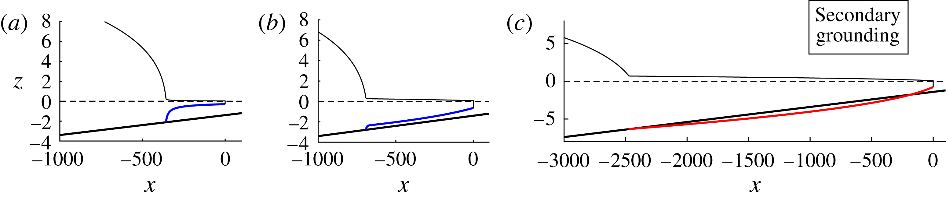
Schematics illustrating the two types of secondary grounding that invalidates a possible steady-state grounding-line position on the basis that the ice shelf necessary to sustain it would penetrate the bedrock, corresponding to one of conditions (6.1a,b ) being satisfied. (a) Type I, where the predicted profile penetrates the bed immediately in front of the grounding line. (b) Type II, where the predicted profile instead penetrates the bed some distance downstream of the grounding line.
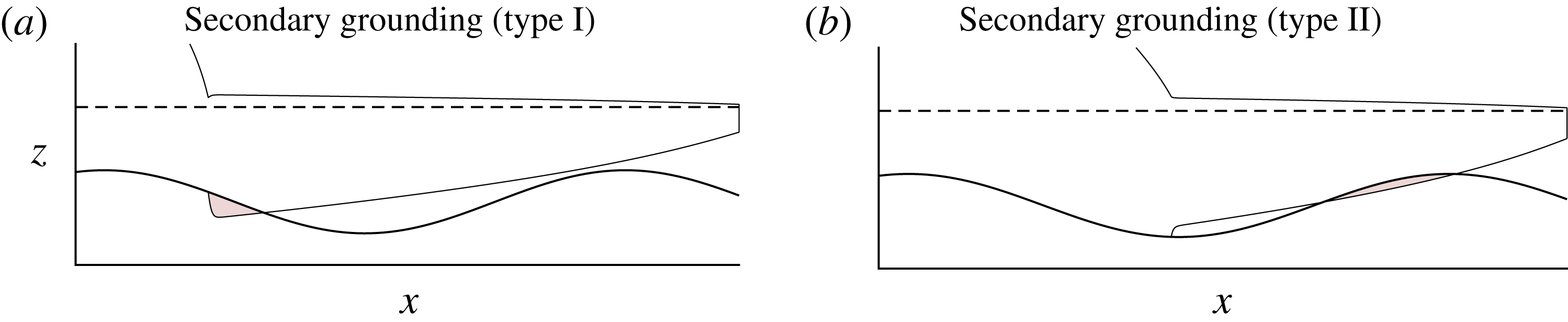
In figure 15, I illustrate the two different types of secondary grounding that are theoretically possible. Panel (a) shows type I, in which the steady ice-shelf profile (5.1) is predicted to penetrate the bed immediately at the grounding line. Panel (b) shows type II, where penetration instead occurs further downstream. Mathematically, the two types occur if
 $$\begin{eqnarray}\displaystyle \left.\begin{array}{@{}cl@{}}H^{\prime }(x_{G})>d^{\prime }(x_{G}) & \text{(type I)},\\ \left.\begin{array}{@{}c@{}}H^{\prime }(x_{G})<d^{\prime }(x_{G}),\\ \text{and }H(x)>d(x)\;\text{for some }x>x_{G}\end{array}\right\} & \text{(type II)},\end{array}\right\} & & \displaystyle\end{eqnarray}$$
where
 $H$
is the thickness profile of the ice shelf resulting from the assumption of continuous flotation. It should be noted that type-II secondary grounding forms a necessary condition for the formation of a so-called ice rise or rumple, which is a localised region of the ice shelf that contacts the bedrock downstream of the primary grounding line. However, it is not a sufficient condition because the resulting (typically considerable) increase in the buttressing force resulting from a basal contact of the ice shelf will result in a more advanced steady-state grounding line. The advancement of the grounding line resulting from this additional buttressing can close the gap upstream of the position of secondary basal contact where (6.1b
) is satisfied, implying that an ice rise does not necessarily form in steady state despite the prediction of type-II secondary grounding.
The inducement of type-I secondary grounding (6.1a ) can result in a special form of grounding-line advancement in which the ice shelf ‘regrounds’ continuously in front of the present grounding line. This mode of grounding-line advancement differs from the more typical mode of migration controlled by thickening of the ice sheet on the grounded side of the grounding line. It can also result in the formation of an extended grounding region, an aspect reserved for dedicated treatment as part of the companion paper (Pegler Reference Pegler2018).
The steady-state grounding-line position
 $x_{G}$
as a function of
 $S$
for (a)
 $\unicode[STIX]{x1D6FC}=-2\times 10^{-3}$
and
 $\unicode[STIX]{x1D6FD}=2.8$
, and (b)
 $\unicode[STIX]{x1D6FC}=2\times 10^{-3}$
and
 $\unicode[STIX]{x1D6FD}=1.4$
. The grounding-line positions for which the steady-state solution results in secondary grounding (SG) is shown by the blue shading in each case. These regions were determined using the method of finding the steady-state solutions subject to the critical cotangency condition (6.2) described in § 6. Type-I secondary grounding (6.1a
) is shown as a lighter shade and type-II (6.1b
) is shown by the darker shade. In case (b), there is a critical value
 $S_{\ast }\approx 6.9\times 10^{-4}$
, for which no steady state exists for all
 $S>S_{\ast }$
because of its invalidation by secondary grounding.
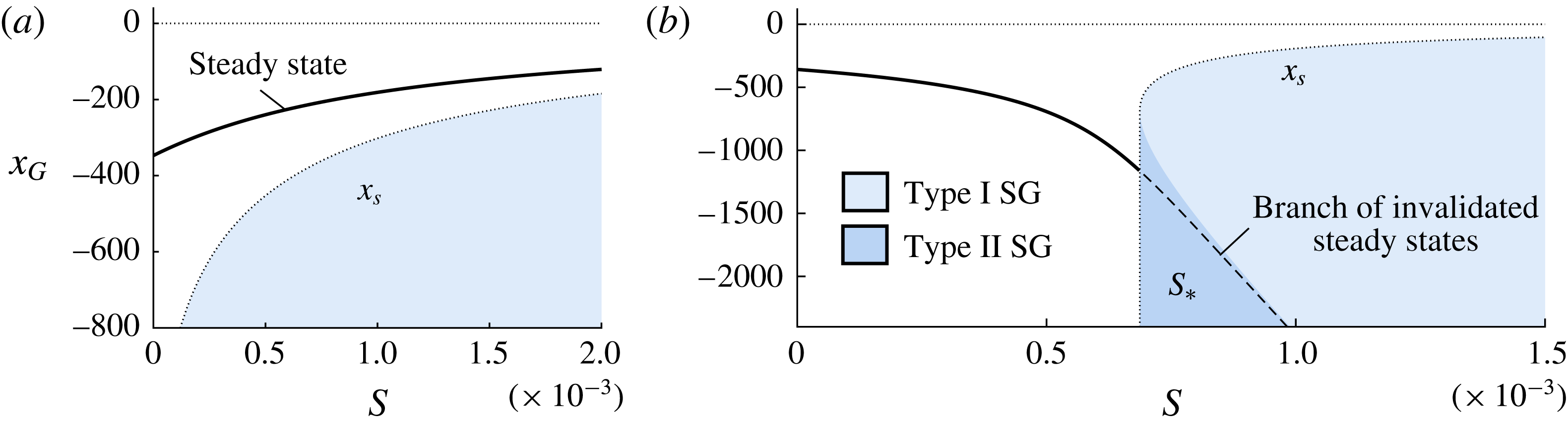
The critical regions of the space
 $(S,x_{G})$
where secondary grounding occurs can be examined by first determining the ‘locus’ over this space for which the ice shelf is critically cotangent with the bedrock at the grounding line,
 $$\begin{eqnarray}\displaystyle H(x_{S})=d(x_{S}),\quad \text{and}\quad H^{\prime }(x_{S})=d^{\prime }(x_{S}). & & \displaystyle\end{eqnarray}$$
The curve of
 $x_{S}(S)$
provides both the boundary of the region for which secondary grounding occurs as well as the boundary of the critical switch from type I to type II. The curve of
 $x_{S}(S)$
is generally multi-valued and hence it is easier to specify
 $x_{G}=x_{S}$
and determine the critical drag parameter
 $S(x_{S})$
for which (6.2a,b
) are mutually satisfied. For general
 $n$
, this curve can be determined numerically by solving (3.1b
) subject to (6.2a,b
) and iterating
 $S$
bisectively until (3.2b
) is adequately satisfied. For
 $n=1$
, this curve can instead be obtained analytically by using the first-integral of (3.1b
), namely,
 $$\begin{eqnarray}4Hu^{\prime }+S(x_{C}-x)={\textstyle \frac{1}{2}}\unicode[STIX]{x1D6FF}H^{2}\end{eqnarray}$$
(Pegler Reference Pegler2016). Using the steady-state expression for the derivative,
 $u^{\prime }=-H^{-2}H^{\prime }$
, substituting the cotangency conditions of (6.2a,b
) directly into (6.3) and rearranging, I obtain
 $S(x_{S})=((1/2)d^{2}+4d^{3}d^{\prime })/(x_{C}-x_{S})$
. The implied regions for which type-I and type-II secondary grounding occur are shown by the lighter and darker shaded regions in figure 16, respectively.
For the negative sloped example of figure 16(a),
 $x_{S}<x_{G}$
, and hence secondary grounding does not interfere with the validity of any steady states. For the positive-slope case of figure 16(b), satisfaction of (6.1a,b
) occurs only for
 $S>S_{\ast }$
, where
 $S_{\ast }=S_{\ast }(\unicode[STIX]{x1D6FC},\unicode[STIX]{x1D6FD})\approx 6.9\times 10^{-4}$
is a critical drag parameter. The sharp ‘switch-on’ of secondary grounding at
 $S_{\ast }$
abruptly removes a significant branch of consistent steady-state grounding-line positions. These invalidated steady states are indicated by a dashed curve in figure 16(b). This invalidation explains the lack of any steady state in the numerical example of figure 4(d), for which
 $S=2\times 10^{-3}$
is greater than
 $S_{\ast }$
. The critical inducement of secondary grounding by lateral stresses produces a distinct process of grounding-line control that is additional to the direct effect of ice-shelf buttressing generated by the integral of lateral stresses. The implications of this phenomenon for marine ice sheet structure, grounding-line migration, and the suppression of otherwise destabilising grounding-line retreat will be addressed as part of the companion paper (Pegler Reference Pegler2018).
7 Illustrating the determination of ice-sheet balances
The two mechanically distinct effects of lateral stresses described in this paper are, first, its direct generation of ice-shelf buttressing and, second, its inducement of secondary grounding. The analyses of §§ 4 and 6 addressed these effects individually. In order to determine the consistent steady-state grounding-line positions for a given topography, it is necessary to consider these phenomena in tandem. This section brings the different mathematical machineries used to analyse these two phenomena together in application to establishing the consistent balances possible for an illustrative nonlinear bedrock topography. For demonstration, I consider
 $n=3$
and a basal topography with a double bump defined by
 $$\begin{eqnarray}b(x)=\text{e}^{-\unicode[STIX]{x1D709}^{2}}(\unicode[STIX]{x1D6FC}\unicode[STIX]{x1D709}^{2}+\unicode[STIX]{x1D6FE}\unicode[STIX]{x1D709})-\unicode[STIX]{x1D6FD},\quad \text{where}~\unicode[STIX]{x1D709}\equiv (x/k)-\unicode[STIX]{x1D709}_{0},\end{eqnarray}$$
 $\unicode[STIX]{x1D6FC}=4\text{e}$
,
 $\unicode[STIX]{x1D6FD}=9$
,
 $\unicode[STIX]{x1D6FE}=-1$
,
 $k=10^{3}$
and
 $\unicode[STIX]{x1D709}_{0}=3$
, which is illustrated in figure 17(b).
Panel (a) shows the steady-state grounding-line positions
 $x_{G}$
predicted by (4.2) for the nonlinear bed topography (7.1) and the rheological exponent
 $n=3$
as a function of drag parameter
 $S$
. The regions in which secondary grounding (SG) invalidates the consistency of a steady state are shown by the blue shaded regions; type I and type II are shown by the lighter and darker shades, respectively. The steady states invalidated by secondary grounding are shown as dotted curves. The solution to the full system (3.1), (3.2) reveals additional steady-state branches shown as red curves. Panel (b) shows the bed topography (7.1) and its intersections with the horizontal line
 $z=-d_{0}(1-\unicode[STIX]{x1D6FF})$
(dashed) producing the four steady states possible for zero buttressing,
 $S=0$
. Panel (c) shows the state involving a secondary contact with the bedrock, corresponding to the position of the blue circle in (a).
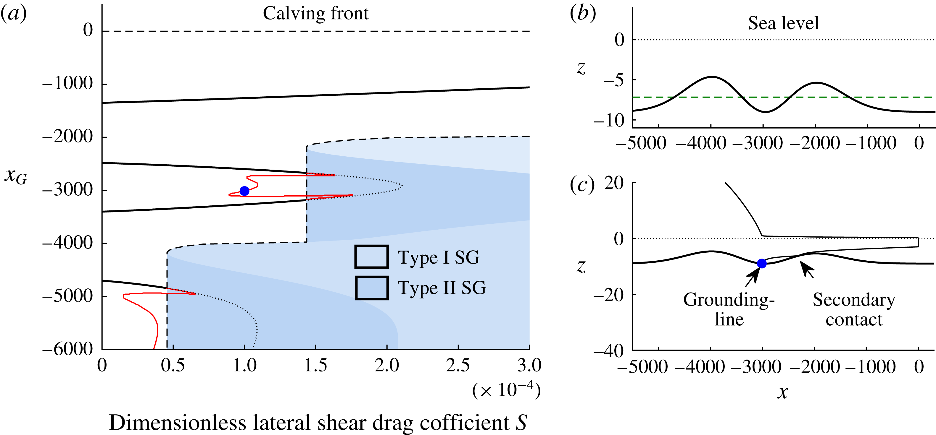
7.1 Steady states and the removal of hysteresis
The first step is to determine the solutions to the grounding-line equation (4.2) with the expressions for the extensional-resistance function (A 1) and the buttressing function (4.13), for
 $x_{G}$
. Solving this algebraic equation using a numerical root finder, I obtain the steady-state grounding-line position
 $x_{G}$
as a function of
 $S$
shown as a thick solid curve in figure 17(a). With the candidate steady states determined, the second step is to determine which are rendered inconsistent by secondary grounding. To determine the locus of critical grounding-line positions for which secondary grounding occurs, I apply the numerical method outlined below (6.1). The grounding-line positions that would be affected by secondary grounded are overlaid on figure 17(a) in blue, with types I and II shown by the lighter and darker shades, respectively. The invalidated steady states are shown as dotted curves extended into the blue region.
For the unconfined case,
 $S=0$
, equation (4.2) reduces to
 $d(x)=d_{0}=7.96$
. The solutions to this equation represent the intersections between
 $b(x)$
and the line
 $z=-d_{0}(1-\unicode[STIX]{x1D6FF})$
, shown in figure 17(b). There are a total of four such states. As
 $S$
is increased, the first effect of lateral stresses is to cause the unbuttressed steady states on positive bed slopes to move backwards and those on negative bed slopes to move forwards. Another effect is to introduce a fifth steady state far upstream (not shown). At certain critical values of
 $S$
, certain pairs of steady states meet and ‘annihilate’ one another. The annihilations represent saddle-node bifurcations, which are a feature of dynamical systems with multiple steady states. The solutions near the bifurcation points in this example are invalidated by type-II secondary grounding causing an intersection between the ice shelf and one of the topographic maxima. The invalidations occur sharply at critical values given by
 $S=4.6\times 10^{-5}$
and
 $S=1.4\times 10^{-4}$
. For values of
 $S>1.4\times 10^{-4}$
, there is just one steady state remaining.
The existence of multiple steady states (there can be a total of five in the example above) implies the possibility for hysteresis effects, where the system will be attracted to a different state depending on its initial condition. For example, if a change in climate were to induce a reduction in ice flux
 $Q$
, a grounding-line retreat can be stimulated. If the flux were to reinstate in future then, if the grounding line has migrated upstream of an unstable steady state, then it will not return to its former state. Instead, it will continue to retreat upstream, potentially leading to either irreversible runaway retreat or stabilisation towards a new position further upstream. The steady-state plot of figure 17 shows that, with just one stable state remaining for
 $S>1.4\times 10^{-4}$
, lateral stresses have the effect of removing the possibility for hysteresis. Above this value, the system converges unconditionally towards this stable steady state. Above this threshold, the possibility for hysteresis has been eliminated. A general analysis of the conditions necessary to maintain the global stability of a marine ice sheet under the effects of ice-shelf buttressing and secondary grounding forms the subject of the companion paper (Pegler Reference Pegler2018).
7.2 Steady secondary contact
An ice rise or rumple represents a localised region of contact between an ice shelf and the bedrock downstream of the primary grounding line. The position of the primary grounding line and the ice rumple for such a state are not predicted by (4.1) because of the underlying assumption that the ice shelf forms a single region of flotation. To inspect the possibility of states that sustain a region of secondary grounding in steady state, I conducted a comprehensive search of the solutions to the full steady-state equation (3.1). This was achieved using a method of shooting over the thickness upstream, and iterating it bisectively until the frontal stress condition (3.2) is adequately satisfied. Unlike the solutions based on (4.2) alone, this general method of solution describes several additional solutions involving two disjoint regions of flotation. The additional branches of steady states are shown as red curves in figure 17(a). The additional solutions initially appear to continue the branch of solutions of the steady states with a fully floating ice shelf for values of
 $S$
above the critical values at which secondary grounding switches on, before abruptly turning back at saddle-node bifurcations. New solutions involving a secondary contact can occur for values of
 $S$
both above the threshold at which secondary grounding is predicted and below it. The profile of such a state, occurring at the blue circle in figure 17(a), is shown in figure 17(c). The solution exhibits a brief ‘glancing’ contact with the bedrock, which can be interpreted as an ice rumple. Thus, multiple additional steady states can be produced by allowing for a secondary contact. As shown in figure 17(c), the contacts create a sharp jump in the thickness gradient of the ice shelf between the start and end of the secondary region of contact, implying a considerable impact of the contact on the morphology of the ice shelf. This includes a considerable thickening of the region of the ice shelf between the point of secondary contact and the grounding line. Assuming an alternating pattern between stable and unstable states, I anticipate that a subset of these additional states are stable and the others unstable. By contributing to a larger interior thickness, lateral stresses can thus induce the development of an ice rise or rumple. A dedicated analysis could be conducted to investigate the local stability of these additional states and is left for future consideration.
8 Geophysical discussion and model applicability
This section discusses the physical implications of lateral stresses within the geophysical context and summarises the limitations of the model.
8.1 The variation in parametric control of the grounding line
In order to visualise the new parametric dependences introduced by lateral stresses in the general balance equation (4.2), it is insightful to express it in its dimensional form. With the power-law results of (A 2) and (4.14) incorporated, this equation reads
 $$\begin{eqnarray}\underbrace{4\left[\frac{(MQ)^{n+1}C_{-}^{n}}{\unicode[STIX]{x1D707}_{0}^{n}}H_{G}^{(n^{2}-3n-1)}\right]^{1/n^{2}}}_{\text{Extensional resistance}}+\underbrace{\frac{\unicode[STIX]{x1D6FF}}{2}\left(\frac{M^{\prime }Q}{\unicode[STIX]{x1D6EC}}\right)^{2/n+1}\hat{B}\left(\frac{x_{G}}{\unicode[STIX]{x1D6EC}},\frac{x_{C}}{\unicode[STIX]{x1D6EC}}\right)}_{\text{Ice\text{-}shelf buttressing resistance}}=\frac{\unicode[STIX]{x1D6FF}}{2}H_{G}^{2},\end{eqnarray}$$
where
 $H_{G}\equiv d(x_{G})$
is the grounding-line thickness,
 $M\equiv (\unicode[STIX]{x1D707}_{0}/\unicode[STIX]{x1D70C}g)^{n}$
,
 $M^{\prime }\equiv (\unicode[STIX]{x1D707}_{0}/\unicode[STIX]{x1D70C}g^{\prime })^{n}$
,
 $\hat{B}$
is the dimensionless form of the buttressing force given by (4.13) or (4.14), which depends purely on the geometrical specification of the ice shelf, and
 $\unicode[STIX]{x1D6EC}\equiv (\unicode[STIX]{x1D706}_{+}w^{n})^{1/(n+1)}$
is a length formed from the channel half-width
 $w$
. For negligible softening and
 $n=3$
, for example,
 $\unicode[STIX]{x1D6EC}=0.47\,w$
. Equation (8.1) shows that the extensional resistance and ice-shelf buttressing forces depend individually on the grounding-line flux
 $Q$
. Therefore, the relationship between
 $Q$
and thickness
 $H_{G}$
depends on the solution of the implicit algebraic equation (8.1). With
 $Q=q(x_{G})$
represented in terms of the grounding-line position using (2.20) and
 $H_{G}=d(x_{G})$
equated to the bedrock flotation profile, equation (8.1) forms an algebraic equation that can be solved directly for the steady-state grounding-line position
 $x_{G}$
.
For zero buttressing,
 $B=0$
, equation (8.1) can be rearranged to give
 $$\begin{eqnarray}Q\approx \frac{1}{M}\left[\left(\displaystyle \frac{\unicode[STIX]{x1D6FF}}{8}\right)^{n^{2}}\left(\frac{\unicode[STIX]{x1D707}_{0}}{C_{-}}\right)^{n}H_{G}^{(n^{2}+3n+1)}\right]^{1/(n+1)}\quad \text{(unbuttressed)},\end{eqnarray}$$
which recovers the unbuttressed relationship for grounding-line flux for a sliding ice stream (Schoof Reference Schoof2007b ). In the opposing limit of strong buttressing, equation (8.1) predicts the distinct expression
 $$\begin{eqnarray}Q\approx \frac{\unicode[STIX]{x1D6EC}^{n+1}}{M^{\prime }(Nl)^{n}}H_{G}^{n+1}\quad \text{(strongly buttressed)},\end{eqnarray}$$
where
 $N\equiv (n+1)/n$
and
 $l\equiv x_{C}-x_{G}$
is the shelf length. For the purpose of illustrating the new parameter dependences arising for strong buttressing mathematically, I have here neglected the contributions to
 $\hat{B}$
due to
 $H_{C}$
(though it should be noted that this is not a good approximation in general and can be straightforwardly retained). The result of (8.3) illustrates that the calving position
 $x_{C}$
, as contained in the shelf length
 $l$
, and the half-width of the ice shelf,
 $w\propto \unicode[STIX]{x1D6EC}$
become central controls. Further, the absence of
 $C_{-}$
in (8.3) shows that basal conditions have no important effect on the dynamics of a sufficiently buttressed grounding line, thus confirming the control illustrated earlier in figure 11.
The removal of a dependence of the grounding line on the basal stress clarifies that the control of a marine ice sheet is based on two distinct physical processes: one is the control of the grounding-line position; the other is the control of the degree of ‘pile-up’ upstream of that position. Importantly, the physics controlling these independent processes result in two necessary physical conditions for maintaining a large marine ice sheet: one is to support a sufficiently advanced grounding line; the other is to sustain a sufficient drag on flow in the grounded region. The failure of either one of these physical constraints can form a ‘weak link’ that is sufficient for collapse of a marine ice sheet. It might be anticipated that the maintenance of an advanced grounding line is the weakest of these two links for sustaining the WAIS. The split in necessary physical conditions for maintaining a marine ice sheet explains why lateral stresses in an ice shelf are so much more important than those in the grounded region. Since ice-shelf buttressing directly provides an independent control of the grounding line, with a magnitude of force that can readily exceed the extensional resistance to flow across a grounding line relied upon in the absence of buttressing, it has a direct impact on the sustainment of the first of these weak-link conditions (the sustainment of an advanced grounding line). Lateral stresses in the grounded region, by contrast, only significantly influence the second necessary condition representing the sustainment of a thick and steep ice sheet upstream of the grounding line. This separation of physical controls explains why the maintenance of a stable marine ice sheet can be dictated by the sustainment of ice-shelf buttressing.

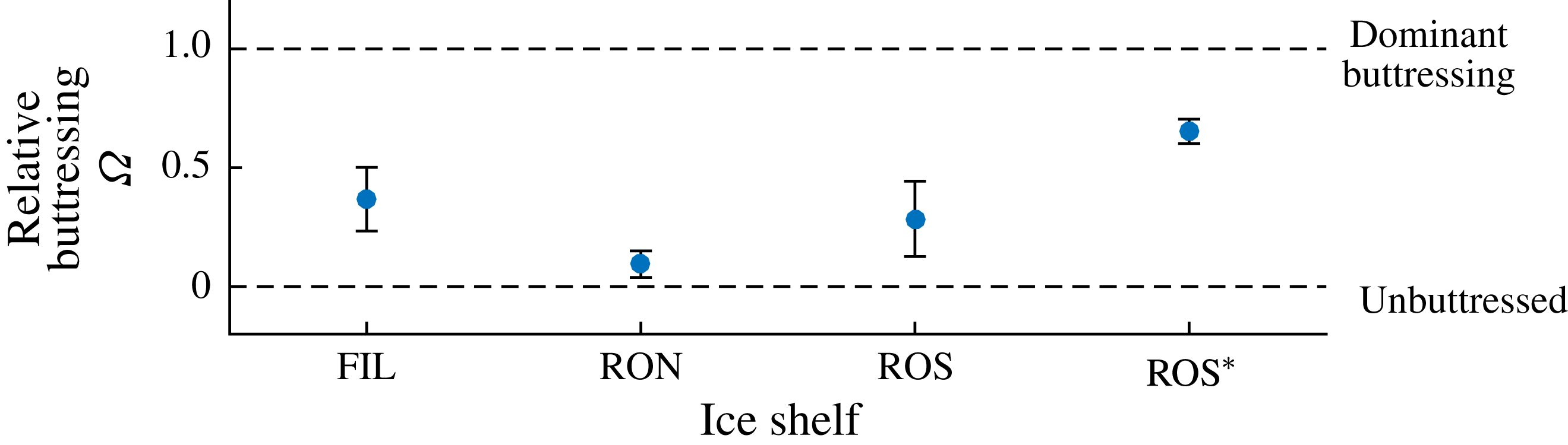
Estimates of the thickness at the grounding line
 $d$
, distance between grounding line and calving front
 $l$
, ice-shelf width
 $w$
and volumetric flux per unit width
 $Q$
for five ice-shelf regions. The given ranges for
 $d_{G}$
and
 $w$
encompass variations in values for a given ice shelf. The relative buttressing parameter
 $\unicode[STIX]{x1D6FA}$
evaluated using (8.4) is listed in the final column.

8.2 Assessing the significance of ice-shelf buttressing
To indicate the locations of a selection of ice shelves on the spectrum of relative buttressing strength, I evaluate the parameter
 $\unicode[STIX]{x1D6FA}$
, defined by (4.5). Using the analytical result of (4.13) for power-law fluid and negligible net accumulation,
 $\unicode[STIX]{x1D6FA}$
can be evaluated as
 $$\begin{eqnarray}\unicode[STIX]{x1D6FA}\equiv \frac{B}{{\textstyle \frac{1}{2}}\unicode[STIX]{x1D70C}g^{\prime }d_{G}^{2}}=\frac{1}{d_{G}^{2}}\left[\left(\frac{\unicode[STIX]{x1D707}_{0}}{\unicode[STIX]{x1D70C}g^{\prime }}\right)^{n}\frac{Q}{\unicode[STIX]{x1D6EC}}\right]^{2/(n+1)}\left[\left(H_{C}^{N}+\frac{Nl}{\unicode[STIX]{x1D6EC}}\right)^{2/N}-H_{C}^{2}\right].\end{eqnarray}$$
The relative buttressing
 $\unicode[STIX]{x1D6FA}$
is evaluated for a selection of ice-shelf systems listed in table 1. The main central component of the Ross ice shelf is considered separately to its smaller, channelised component east of Roosevelt Island (denoted ROS
 $^{\ast }$
). The predicted
 $\unicode[STIX]{x1D6FA}$
are listed in the final column and plotted in figure 18. Significant variations in its value are apparent. The smallest
 $\unicode[STIX]{x1D6FA}$
applies to the Ronne ice shelf, with
 ${<}$
15 % of its resistance stemming from buttressing. This may be attributable to its considerable width, which reduces the transverse shear stresses. The largest
 $\unicode[STIX]{x1D6FA}$
applies to the confined region of the Ross ice shelf for which 65 % of grounding-line resistance is predicted to stem from buttressing.
8.3 Applicability
On the basis of the numerical comparisons given in the supplementary document, it is likely that the model describes a large range of marine ice sheet configurations from those channelised in fjords in addition to larger, broader ice shelves. However, a number of caveats should be noted. Primary anticipated limitations include: the existence of islands or ice rises, which will change the buttressing forces generated by the ice shelf; the more complex two-dimensional flow that may be generated by strongly localised ice-stream inputs, which can be more typical for large ice shelves; and the effects of significant transverse variations in basal conditions. A limitation of the steady-state results, as represented by the general balance equation (8.1), is their accuracy if the ice shelf or grounding line are sufficiently unsteady.
The examples of this study have focused on certain specialised situations. These include the assumption of a localised input directly at the ice divide specified by (2.19), and the assumption of a uniform basal coefficient of drag and flow width. These assumptions have been made for the sake of illustrating the results and can all be relaxed within the steady-state framework developed, which is more versatile than the specifications considered in these examples. The framework can also accommodate more complex rheological specifications, basal conditions and calving laws. With these generalisations, the framework provides an efficient complement to direct numerical analysis, with the numerical saving affording scope for thorough exploration of scenarios and sensitivity analysis in case studies.
9 Conclusions
This paper has explored the effects of lateral stresses on the dynamics of marine ice sheets. The primary result is an analytical toolkit for determining steady-state grounding-line positions, which affords excellent agreement with the predictions of full horizontally two-dimensional numerical simulation with a numerical expense that is many orders of magnitude smaller. The analysis elucidates the steady-state regimes of grounding-line control, and its relationship to ice-sheet flow and force-balance structure, across a complete spectrum of relative buttressing strength. The possibility for dominant control of the grounding line by the ice shelf was determined even when lateral stresses are considerably weaker than the resistive stresses exerted upstream of the grounding line. A distinct secondary mechanism of grounding-line control by lateral stresses via its inducement of further basal contacts between an ice shelf and the bedrock was also demonstrated. This effect was shown to provide a further mechanism for the stabilisation of a grounding line that is entirely additional to the effect of the ice-shelf buttressing generated already by the lateral stresses without basal contact. The results provide essential groundwork necessary to understand the conditions for tipping to and recovery from marine ice sheet instability, which forms the subject of the companion paper (Pegler Reference Pegler2018).
The reduced equation for steady-state grounding lines (8.1) incorporates the buttressing force and extensional stresses resisting flow at the grounding line simultaneously using universal analytical expressions of grounding-line thickness and shelf length, respectively. Analysis of the solutions shows that lateral stresses fundamentally alter the characteristics of grounding-line control from an extension-dominated balance for weak buttressing to a buttressing-dominated balance. For sufficient buttressing, the extensional dynamics that dominates the resistance across an unbuttressed grounding line can become negligible. There is therefore a complete transition in dynamical control from the ice shelf playing no role in unbuttressed dynamics to a completely dominant role for even a relatively short confined ice shelf. The approximate position of a steady-state grounding line can lie close to the location where the interior lateral-drag-dominated region of the ice shelf intersects the bedrock on extrapolation, implying that the control of the grounding line is being dominated independently by the profile of the ice shelf. There is then no relationship between the control of the grounding line and the mechanics of the grounded region other than the flux of mass across the grounding line. Basal lubrication can completely lose its effect on the grounding line for sufficient buttressing, with the potential for the grounding line to be completely unchanged even when basal stresses are entirely removed (see figure 11). From the perspective of the ice sheet as a whole, lateral stresses on the ice shelf can thereby largely independently set the position and ice-sheet thickness at the grounding line, with the role of basal stress, and the lateral stresses exerted on the grounded region, being primarily to control the degree of thickening of the ice sheet as one moves upstream of the grounding line.
As lateral stresses are incorporated, the ice-shelf structure transitions from the classical extension-dominated concave solution (van der Veen Reference van der Veen1983) towards the regime involving a wedge-shaped lateral-drag-dominated solution connected to the grounding line through an inlet boundary layer involving significant extension (Pegler Reference Pegler2016). The characteristics of this structure arise even when ice-shelf buttressing is present but not necessarily the dominant resistance to flow across the grounding line. A parameter
 $\unicode[STIX]{x1D6FA}$
was formulated to measure the relative significance of ice-shelf buttressing as a proportion of the total resistance to grounding-line flow (with the rest provided by the extensional viscous stress). The value of the relative buttressing was determined to be related in a simple way to features of the ice-shelf structure via an expression (5.4) involving the grounding-line thickness, the calving-front thickness and the thickness just downstream of the input boundary layer.
The second main result was to determine a distinct effect of lateral stresses of inducing an ice shelf to make further basal contacts downstream of the grounding line. This phenomenon of ‘secondary grounding’ invalidates the steady-state grounding-line positions that are otherwise consistent with the grounding-line balance equation applicable for an ice shelf with a single region of continuous flotation (8.1). There is therefore a sharp switch-on of differing stability properties subject to the satisfaction of a critical condition. Despite it not necessarily requiring strong buttressing to arise, the controlling influence of secondary grounding is, like the lateral-stress-dominated regime, determined independently by the dynamics of the ice shelf. The implications of this mechanism for suppressing the unstable retreat of grounding lines will form an aspect explored in the companion paper.
By combining the predictions of the grounding-line balance equation with conditions for secondary grounding, the positions of consistent steady states for a generic one-dimensional topography are determined. For an example nonlinear bedrock, it was shown that steady-state branches of the stability diagram progressively disappear as lateral stresses are incorporated. The steady states can disappear either at saddle-node bifurcations or at the ‘switch-on’ of secondary grounding. The possibility of secondary grounding downstream was found to produce multiple additional steady states involving a brief ‘glancing’ contact with the bedrock in the manner of an ice rise. Under this effect, a rich variety of additional steady-state regimes are revealed. For sufficiently large lateral stresses, only one steady state survives. In this case, the ice sheet can be expected to approach this steady state unconditionally, with the possibility of irreparable hysteresis effects, of the kind identified previously in the context of unbuttressed grounding-line dynamics, being eliminated. The critical loss of a steady state dependent on buttressing following parametric variation is generally more likely to result in the crossing of a globally unique tipping point, indicating that an abrupt and permanent switch to large-scale collapse may be more likely for a buttressing-controlled tipping point than an unbuttressed tipping point, where restabilisation upstream may be more likely.
By considering the relative buttressing
 $\unicode[STIX]{x1D6FA}$
in the context of a selection of ice-shelf systems, it was found that they generally lie intermediate to the end members of the spectrum of relative buttressing strength. A majority contribution from buttressing arises for the channelised section of the Ross ice shelf, but considerably weaker relative buttressing is predicted for the Ronne ice shelf. These estimates indicate that the controls provided by ice-shelf buttressing are likely to be of broad importance to the geophysical context.
By considering the stability of a marine ice sheet in terms of two physically distinct necessary conditions – one based on grounding-line control, the other based on the degree of ‘pile-up’ upstream of that position – it can be explained why even slight lateral contact of an ice shelf introduces a leading control of the large-scale stability and mass balance of a marine ice sheet. From the perspective of the entire ice sheet, the drag stresses owing to lateral stresses on the ice shelf are generally much smaller in magnitude compared to those exerted by basal drag along the grounded interior of the ice sheet and, moreover, are likely to constitute a tiny contribution to the total drag exerted through the length of the ice sheet. However, by virtue of its exertion at the grounding line and direct resistance to flow across it, it is readily possible, despite their small magnitude overall, for lateral stresses on an ice shelf to impact the large-scale stability of the ice sheet. The reason is that the resistive force provided by ice-shelf buttressing can readily exceed the relatively weak extensional stress that would provide the only resistance to flow across the grounding line in its absence. The simple structural link between the drag-dominated profile of the ice shelf and the grounding line determined in § 5 clarifies this emergent control. Variations in external parameters associated with ice-shelf preservation, such as the control of its calving position, basal melting and lateral conditions are thus likely to constitute leading-order processes governing large-scale marine ice sheet dynamics and stability. Understanding the details of these processes and resolving them accurately within models is thus vital if we are to predict future sea levels and the potential for collapse of the West Antarctic Ice Sheet with confidence.
Acknowledgements
I am grateful to B. Minchew, A. Robel and G. Worster for helpful comments and discussions on this work. I am also grateful for the work of three anonymous referees whose comments led to significant improvement of the paper. I thank H. Gudmundsson for developing and providing his finite-element solver Úa which I used to benchmark the predictions of the theory, as presented in the supplementary document.
Supplementary material
Supplementary material is available at https://doi.org/10.1017/jfm.2018.741.
Appendix A. Analytical descriptions of steady grounding-line forces
This appendix develops generalisations of the analytical forms of the ‘database functions’
 $E(d)$
and
 $B(x_{G},x_{C})$
, defined by (4.3) and (4.10), respectively. The results yield the general equation (8.1).
A.1 The generalised extensional-resistance function
To extend the approach of § 4.1 to
 $n\neq 1$
, I first determine the universal shape profile of the grounded region by numerically integrating (3.1) forwards subject to an arbitrary upstream thickness. The resulting profile is used to construct the gradient function
 $\unicode[STIX]{x1D701}(H)$
and, in turn, the extensional-resistance function
 $E(d)$
using (4.3). With
 $E(d)$
in hand for
 $n=3$
, the special unbuttressed dimensionless grounding-line thickness
 $d_{0}\approx 7.96$
is determined by solving
 $E(d)=(\unicode[STIX]{x1D6FF}/2)d^{2}$
using a numerical root finder.
To develop an almost exact analytical approximation for
 $E(d)$
, I follow § 4.1.2 and approximate the flow in the grounded region using a drag-dominated balance to obtain
 $D(u)\equiv \unicode[STIX]{x1D70F}_{b}(u)+H\unicode[STIX]{x1D70F}_{s}(u)=-H(H^{\prime }+b^{\prime })$
, where
 $D(u)$
is used to represent the combined drag on the flow in the grounded region owing to both basal and lateral drag. Using this expression to substitute for
 $H^{\prime }$
in (4.3), with
 $\unicode[STIX]{x1D707}=(-H^{-2}H^{\prime })^{(1/n)-1}$
, I obtain
 $$\begin{eqnarray}\displaystyle E & {\approx} & \displaystyle 4d^{(n-2)/n}\left(b^{\prime }+\frac{D(u)}{d}\right)^{1/n}\end{eqnarray}$$
 $$\begin{eqnarray}\displaystyle & {\approx} & \displaystyle 4d^{(n^{2}-3n-1)/n^{2}},\end{eqnarray}$$
where
 $u=1/d$
and the second result is the reduced form of (A 1) applicable for sufficiently small
 $b^{\prime }$
(for which the expression is reduced to a pure function of grounding-line thickness
 $E(d)$
) and for negligible contributions to the total drag in the grounded region owing to lateral stresses,
 $D(u)\approx \unicode[STIX]{x1D70F}_{b}(u)=d^{-1/n}$
. By comparing the result of (A 2) with my numerically determined version of
 $E(d)$
, I obtain excellent agreement for all
 $d\geqslant d_{0}$
. The largest error occurs for the unbuttressed balancing thickness
 $d_{0}$
, namely,
 $d=d_{0}\approx (8/\unicode[STIX]{x1D6FF})^{r}$
, where
 $r\equiv n(n+1)/(n^{2}+3n+1)$
. This ‘worst-case’ error is within just 0.1 % of the numerically determined value, indicating that the analytical prediction given by (A 1) can be treated as a practically exact general approximation.
A.2 The generalised buttressing force with melting
The analytical approximation for the buttressing force is obtained by substituting an analytical solution for the prevailing region of the ice shelf downstream of the inlet boundary layer (Pegler Reference Pegler2016) into the buttressing integral (4.10). First recall the lateral-drag-dominated flow approximation (5.3), which for power-law fluid reads
 $$\begin{eqnarray}\unicode[STIX]{x1D70F}_{s}(u)=S[q(x)/H]^{(1/n)}=\unicode[STIX]{x1D6FF}H^{\prime }.\end{eqnarray}$$
Here I have allowed for a spatially varying flux
 $q(x)=\int _{x_{0}}^{x_{D}}F(x^{\prime })\,\text{d}x^{\prime }$
in order to incorporate the effect of distributed melting along the underside of the ice shelf. Integration of (A 3) subject to the frontal stress condition (3.2b
) yields the general solution describing the prevailing region of the ice shelf downstream of the inlet boundary layer,
 $$\begin{eqnarray}H_{U}=\left(\frac{N}{\unicode[STIX]{x1D6FF}}\int _{x}^{x_{C}}Sq(x^{\prime })^{(1/n)}\,\text{d}x^{\prime }+H_{C}^{N}\right)^{1/N},\end{eqnarray}$$
where
 $N\equiv (n+1)/n$
and
 $H_{C}=[8q(x_{C})]^{1/N^{2}}$
. Using (A 4) to evaluate
 $H(x)$
and
 $u(x)=q(x)/H(x)$
in (4.10), one obtains the result of (4.14). As a shorthand for this calculation, one can use the expression (5.4) with (A 4) used to evaluate
 $H_{U}(x_{G})$
.