 M¯2(Pn,d)
 M2wt
 M2div
 M~2div
 M¯2(Pn,d)





1. Introduction
Moduli problems are of central importance in algebraic geometry. Among them, the moduli spaces
 $\overline {M}_{g,k}({\mathbb P}^n,d)$
of genus
 $g$
degree
 $d$
stable maps into projective space with
 $k$
marked points are particularly important. For example, the Gromov–Witten theory is an intersection theory on these fundamental moduli spaces (introduced and constructed in [Reference KontsevichKon95, Reference AlexeevAle94, Reference Fulton and PandharipandeFP96]).
This article focuses on the deep geometry of the moduli space
 $\overline {M}_{g,k}({\mathbb P}^n,d)$
. By Murphy’s law of Vakil ([Reference VakilVak06]), the moduli space
 $\overline {M}_{g,k}({\mathbb P}^n,d)$
is arbitrarily singular: every singularity of finite type over
 $\mathbb{Z}$
appears for some
 $n$
,
 $g$
, and
 $d$
. The resolution of singularity is arguably one of the hardest problems in algebraic geometry ([Reference HironakaHir64a, Reference HironakaHir64b, Reference de JongdJ96, Reference Abramovich, Temkin and WlodarczykATW20, Reference McQuillanMcQ20], etc.). Several moduli problems offer platforms for geometric solutions, and
 $\overline {M}_{g,k}({\mathbb P}^n,d)$
is one of these (and this is the pivotal motivation for one of us to study the moduli
 $\overline {M}_{g,k}({\mathbb P}^n,d)$
). A canonical resolution of
 $\overline {M}_{g,k}({\mathbb P}^n,d)$
is also desirable for applications computing Gromov–Witten (GW) invariants, even though these invariants can be introduced without using any resolution ([Reference Behrend and FantechiBF97] and [Reference Li and TianLT98]). When the genus
 $g$
is
 $0$
, the moduli space
 $\overline {M}_{0,k}({\mathbb P}^n,d)$
is smooth. For
 $g=1$
, the moduli space
 $\overline {M}_{1,k}({\mathbb P}^n,d)$
is singular and the resolution of the main component of
 $\overline {M}_{1,k}({\mathbb P}^n,d)$
was constructed by Vakil and Zinger in [Reference Vakil and ZingerVZ08]. This was followed by an algebraic approach to the entire moduli space
 $\overline {M}_{1}({\mathbb P}^n,d)$
(without marked points) by Hu and Li [Reference Hu and LiHL10].
Our current article begins to treat the more difficult cases of general genera. We start with the moduli space
 $\overline {M}_2({\mathbb P}^n,d)$
; for conciseness and without loss of generality in terms of singularity, we still work with curves without marked points. The goal of this paper is to geometrically describe a canonical sequence of blowups of
 $\overline {M}_2({\mathbb P}^n,d)$
such that the resulting stack admits only normal crossing singularities and each of its irreducible components is smooth. This is the best that one can hope for as far as smoothness is concerned.
In previous works [Reference Hu and LiHL11, Reference Hu and NiuHN21], the first and third named authors proved that the blowup stacks constructed in both [Reference Hu and LiHL10] and the present article admit modular interpretations: they parameterize certain geometric objects. This perspective has the advantage of being more amenable to generalization to higher genus.
Although not a primary motivation of this series of works, the smooth blowup of
 $\overline {M}_2({\mathbb P}^n,d)$
obtained in this paper can be used, for instance, to prove the ‘hyperplane’ property of the GW invariants of quintic Calabi–Yau threefolds conjectured in [Reference Li and ZingerLZ09] (along with other possible calculations). Further, the method provided in this paper may be helpful for the resolution of other singular moduli used in the recent papers describing progress in mirror symmetry.
To state our main results, consider the smooth Artin stack
 $\mathfrak{M}_2^{{\rm div}}$
(written as
 $\mathfrak D_2$
in [Reference Hu and NiuHN21]) consisting of pre-stable pairs
 $\big (C, D\big )$
where
 $C$
are connected genus 2 nodal curves and
 $D \subset C$
are simple divisors away from the nodes of
 $C$
. A pair
 $(C,D)$
is pre-stable if any smooth rational component of
 $C$
missing the divisor
 $D$
has at least three nodes.
To resolve
 $\overline {M}_2({\mathbb P}^n,d)$
, we construct a sequence of smooth blowups of
 $\mathfrak{M}_2^{{\rm div}}$
, then pull back this sequence to
 $\overline {M}_2({\mathbb P}^n,d)$
. The process would be more straightforward if there existed a natural global morphism from
 $\overline {M}_2({\mathbb P}^n,d)$
to
 $\mathfrak{M}_2^{{\rm div}}$
. Fortunately, although such a global morphism is not available, a rich supply of local morphisms suffices for our purpose.
For every
 $[C,u] \in \overline {M}_2(\mathbb P^n,d)$
, we have
 $\big (C,u^{-1}(H)\big ) \in \mathfrak{M}_2^{{\rm div}}$
for a generic hyperplane
 $H \subset \mathbb P^n$
. Let
 $\breve {\mathbb P}^n = \textrm {Gr}(n,n+1)$
be the space of the hyperplanes of
 $\mathbb P^n$
. Then, for every neighborhood
 $U \subset \overline {M}_2(\mathbb P^n,d)$
of
 $[C,u]$
, we set
 \begin{align} {\bf H}_U:= \big \{H \in \breve {\mathbb P}^n\,:\, \big (C', (u')^{-1}(H)\big ) \in \mathfrak{M}_2^{{\rm div}}\, \forall \,[C',u'] \in U\big \}, \end{align}
which is nonempty as long as
 $U$
is small. Each
 $H \in {\bf H}_U$
gives rise to a morphism
 \begin{align} f_{U,H}:\, U\longrightarrow \mathfrak{M}_2^{{\rm div}}, \quad [C,u]\mapsto \big (C, u^{-1}(H)\big ). \end{align}
We denote by
 \begin{align} \pi : {\mathcal X} \longrightarrow \overline {M}_2({\mathbb P}^n,d),\quad \mathfrak{f}: {\mathcal X} \longrightarrow {\mathbb P}^n \end{align}
the universal family of the moduli
 $\overline {M}_2({\mathbb P}^n,d)$
. The main technical goal of this article is to locally diagonalize the derived objects
 ${\bf R} \pi _* \mathfrak{f}^* {\mathscr O}_{{\mathbb P}^n}(k)$
,
 $k \ge 1$
, in the sense of Definition 2.7.
Theorem 1.1.
There exist a sequence of blowups
 $\widetilde {\mathfrak{M}}_2^{{\rm div}} \longrightarrow \mathfrak{M}_2^{{\rm div}}$
, a Deligne–Mumford stack
 $\widetilde {M}_2(\mathbb P^n,d)$
, and a morphism
 $\widetilde {M}_2(\mathbb P^n,d) \longrightarrow \overline {M}_2(\mathbb P^n,d)$
such that for every small open
 $U \subset \overline {M}_2(\mathbb P^n,d)$
and every
 $H \in {\bf H}_U$
, there exists a commutative diagram

where the horizontal arrow is an isomorphism (of stacks over
 $U$
), and the other two arrows are natural morphisms.
Moreover, the pullback of the derived object
 ${\bf R} \pi _* \mathfrak{f}^* {\mathscr O}_{{\mathbb P}^n}(1)$
to
 $\widetilde {M}_2(\mathbb P^n,d)$
becomes locally diagonalizable. For every integer
 $k \gt 1$
, the pullback of the derived object
 ${\bf R} \pi _* \mathfrak{f}^* {\mathscr O}_{{\mathbb P}^n}(k)$
to the main component
 $\widetilde {M}_2(\mathbb P^n,d)^{\textrm {mc}}$
of
 $\widetilde {M}_2(\mathbb P^n,d)$
is also locally diagonalizable.
Here, the main components
 \begin{align*}\overline {M}_2({\mathbb P}^n,d)^{\textrm {mc}}\subset \overline {M}_2({\mathbb P}^n,d) \quad \textrm {and}\quad \widetilde {M}_2(\mathbb P^n,d)^{\textrm {mc}}\subset \widetilde {M}_2(\mathbb P^n,d)\end{align*}
are, respectively, the irreducible components whose general points are stable maps with smooth domain curves.
The stack
 $\widetilde {M}_2(\mathbb P^n,d)$
is obtained by gluing
 $U \times _{f_{U,H};\,\mathfrak{M}_2^{{\rm div}}} \widetilde {\mathfrak{M}}_2^{{\rm div}}$
for all small open
 $U$
and
 $H \in {\bf H}_U$
. For the precise construction of
 $\widetilde {M}_2(\mathbb P^n,d)$
, see Corollary 5.3.
The case of Theorem 1.1 when
 $k=1$
leads to the following conclusion.
Corollary 1.2.
 $\widetilde {M}_2({\mathbb P}^n,d)$
has smooth irreducible components and, at worst, normal crossing singularities. For
 $d \gt 2$
, the main component is of the expected dimension
 $d(n+1) - n+3$
.
Theorem 1.1 and Corollary 1.2 are proved in Section 5; see Corollary 5.3, Proposition 5.5, and Theorem 5.4. Theorem 1.1 also gives rise to the following statement on the desingularization of the sheaves
 $\pi _\ast \mathfrak{f}^*{\mathscr O}_{{\mathbb P}^n}(k)$
. This is proved in Corollary 5.6.
Corollary 1.3.
Let
 $(\widetilde {\pi }^{\textrm {mc}}, \widetilde {\mathfrak{f}}^{\textrm {mc}})$
be the pullback to
 $\widetilde {M}_2(\mathbb P^n,d)^{\textrm {mc}}$
of the universal family
 $(\pi , \mathfrak{f})$
. Then the direct image sheaf
 $(\widetilde {\pi }^{\textrm {mc}})_{\ast } (\widetilde {\mathfrak{f}}^{\textrm {mc}})^* {\mathscr O}_{{\mathbb P}^n}(k)$
is locally free for all
 $k \ge 1$
. It is of rank
 $kd - 1$
if
 $d \gt 2$
.
As a by-product of the construction of
 $\widetilde {\mathfrak{M}}_2^{{\rm div}}$
, in Proposition 5.7 we construct a Deligne–Mumford stack
 $\widetilde {M}_2(\mathbb P^n,d;k)$
for every integer
 $k \gt 1$
in a manner similar to
 $\widetilde {M}_2(\mathbb P^n,d)$
. The stacks
 $\widetilde {M}_2(\mathbb P^n,d;k)$
, although they are less smooth than
 $\widetilde {M}_2(\mathbb P^n,d)$
, behave more nicely as far as the local diagonalizability of the pullback of the derived object
 ${\bf R} \pi _* \mathfrak{f}^* {\mathscr O}_{{\mathbb P}^n}(k)$
is concerned. The following statement is a recapitulation of Proposition 5.7.
Theorem 1.4.
For every integer
 $k \gt 1$
, the pullback of
 ${\bf R} \pi _* \mathfrak{f}^* {\mathscr O}_{{\mathbb P}^n}(k)$
to
 $\widetilde {M}_2(\mathbb P^n,d;k)$
becomes locally diagonalizable. Moreover, for every irreducible component
 $N$
of
 $\widetilde {M}_2(\mathbb P^n,d;k)$
, with
 $(\widetilde {\pi }_N, \widetilde {\mathfrak{f}}_N)$
denoting the pullback to
 $N$
of the universal family (
1.3
), the direct image sheaf
 $(\widetilde {\pi }_N)_{\ast } (\widetilde {\mathfrak{f}}_N)^* {\mathscr O}_{{\mathbb P}^n}(k)$
is locally free. It is of rank
 $kd - 1$
if
 $d \gt 2$
and the general points of
 $N$
have smooth domain curves.
Our approach to
 $\widetilde {\mathfrak{M}}_2^{{\rm div}}/\mathfrak{M}_2^{{\rm div}}$
improves the technique of [Reference Hu and LiHL10] and combines with the idea of the derived modular. To explain this, notice that the stack
 $\mathfrak{M}_2^{{\rm div}}$
is equipped with a universal curve
 $\rho : {\mathcal C} \to \mathfrak{M}_2^{{\rm div}}$
as well as a universal divisor
 ${\mathcal D} \subset {\mathcal C}$
. We study the parallel diagonalization problem of the derived object
 $\rho _* {\mathscr O}_{\mathcal C}({\mathcal D})$
. Locally over a smooth chart
 $\mathcal V$
of
 $\mathfrak{M}_2^{{\rm div}}$
, the object
 $\rho _* {\mathscr O}_{\mathcal C}({\mathcal D})|_{\mathcal V}$
can be represented by a two-term structural homomorphism
 \begin{align} \varphi : {\mathscr O}_{\mathcal V}^{\oplus m+1} \longrightarrow {\mathscr O}_{\mathcal V}^{\oplus 2}, \end{align}
where
 $m$
is the degree of
 $\mathcal D$
. Throughout this article,
 $m$
can be any positive integer; it corresponds to the case of
 $\pi _*\mathfrak{f}^* {\mathscr O}_{{\mathbb P}^n}(k)$
when
 $m=kd$
.
We provide a detailed analysis of this homomorphism in terms of local modular parameters in Section 2 (and later in Section 4). The analysis of
 $\varphi$
, summarized in Proposition 2.22, guides our construction of the modular blowups in Section 3. The goal is to find global smooth blowups of
 $\mathfrak{M}_2^{{\rm div}}$
such that all the pullback of (1.4) can be diagonalized everywhere, locally. As proved in Section 5, this implies Theorem 1.1 as well as Corollaries 1.2 and 1.3. The procedure involves three rounds, the first and the last of which contain several phases. When the degree
 $d$
is fixed, each round or phase consists of finitely many steps. For conciseness, we hereafter write
 \begin{align} \mathsf r_i,\quad \mathsf p_j,\quad \mathsf s_\ell \end{align}
respectively, for the
 $i$
th round, the
 $j$
th phase, and the
 $\ell$
th step, whenever applicable.
The first round (
 $\mathsf r_1$
) of the modular blowups.

Figure 1. Long description
A diagram illustrating the phases and steps of modular blowups in algebraic geometry. The diagram is organized into five phases, each containing multiple steps. Each phase is labeled with a specific identifier and contains a series of boxes connected by arrows, indicating the progression from one step to the next. The boxes contain various symbols and shapes, representing different elements or states in the modular blowup process. The arrows indicate the directional flow of the process, showing how each step transitions to the next. The weights of the elements are indicated by different shades of gray, with lighter shades representing lower weights and darker shades representing higher weights. The diagram provides a visual representation of the complex relationships and transformations involved in modular blowups, highlighting the structured and sequential nature of the process.
We point out here that, in order to locally diagonalize
 ${\bf R} \pi _* \mathfrak{f}^* {\mathscr O}_{{\mathbb P}^n}(k)$
with
 $k \ge 2$
,
 $(\mathsf r_1\mathsf p_5)$
and
 $(\mathsf r_3\mathsf p_4)$
can be omitted; to locally diagonalize
 ${\bf R} \pi _* \mathfrak{f}^* {\mathscr O}_{{\mathbb P}^n}(k)$
with
 $k \ge 3$
,
 $(\mathsf r_3\mathsf p_3)$
can be omitted as well.
Many sequences of our blowups are performed in the Artin stack
 $\mathfrak{M}_2^{\textrm {wt}}$
of stable weighted curves of genus 2 (i.e. genus 2 nodal curves whose irreducible components are decorated by weights in
 $\mathbb{Z}_{\ge 0}$
, satisfying a certain stability condition; cf. Section 2.1), which comes equipped with the morphisms
 \begin{align} & \mathfrak{M}_2^{{\rm div}} \longrightarrow \mathfrak{M}_2^{\textrm {wt}}, \quad (C,D) \mapsto \big (C, c_1(D)\big ),\nonumber \\ & \varrho : \overline {M}_2({\mathbb P}^n,d) \longrightarrow \mathfrak{M}_2^{\textrm {wt}}, \quad [C,u]\mapsto \big (C, c_1(u^*{\mathscr O}_{{\mathbb P}^n}(1))\big ), \end{align}
where, for every small open
 $U \subset \overline {M}_2({\mathbb P}^n,d)$
and
 $H \in {\bf H}_U$
, the composition of the natural inclusion
 $U \to \overline {M}_2({\mathbb P}^n,d)$
and the latter morphism factors through (1.2) and the former morphism. Each blowup
 $\widetilde {\mathfrak{M}}' \to \mathfrak{M}_2^{\textrm {wt}}$
determines the blowup
 $\mathfrak{M}_2^{{\rm div}} \times _{\mathfrak{M}_2^{\textrm {wt}}}\widetilde {\mathfrak{M}}'$
of
 $\mathfrak{M}_2^{{\rm div}}$
.
1.1 The first round of blowups
 $(\mathsf r_1)$

We first blow up
 $\mathfrak{M}_2^{\textrm {wt}}$
successively along the proper transforms of the substacks that are illustrated in Figure 1 and precisely described in Section 3.1. This round consists of five phases of sequential blowups: the phases are classified by the types of the cores of curves (i.e. the smallest subcurve of genus 2; cf. Definition 2.1) in the corresponding centers as well as the distribution of weights (see Figure 1). Within each given phase, the blowup centers are classified by the number of rational tails attached to the cores (also see Figure 1).
Here, we comment that in
 $(\mathsf r_1\mathsf p_5$
), we treat the case when the core of a curve has weight 1, even though this does not correspond to any point on the main component
 $\overline {M}_2({\mathbb P}^n,d)^{\textrm {mc}}$
. The reason is twofold. First, the structural homomorphism (1.4) is not diagonalized near the corresponding points of
 $\mathfrak{M}_2^{{\rm div}}$
. Since we have reduced the problem of resolving
 $\overline {M}_2({\mathbb P}^n,d)$
to locally diagonalizing (1.4), we shall not specify which points of
 $\mathfrak{M}_2^{{\rm div}}$
miss the image of
 $\overline {M}_2({\mathbb P}^n,d)$
or its main component under (1.2). Second, the underlying weighted curves of the blowup center of
 $(\mathsf r_1\mathsf p_5)$
correspond to some boundary components of
 $\overline {M}_2({\mathbb P}^n,d)$
. As presented in Corollary 1.2, we aim to resolve the entire moduli so that all the components are smooth and meet transversely.
When
 $(\mathsf r_1)$
terminates, we denote the final stack by
 $\widetilde {\mathfrak{M}}^{\mathsf r_1}$
. Every point of
 $\mathfrak{M}_2^{\textrm {wt}}$
has a neighborhood
 $\mathcal V$
such that the pullback
 $\widetilde {\varphi }^{\mathsf r_1}$
of the structural homomorphism
 $\varphi$
of (1.4) to
 $\widetilde {{\mathcal V}}^{\mathsf r_1}={\mathcal V}\times _{{\mathfrak{M}_2^{\textrm {wt}}}}\widetilde {\mathfrak{M}}^{\mathsf r_1}$
has one row that contains an element that divides all other entries of
 $\widetilde {\varphi }^{\mathsf r_1}$
in that row (in such a case, we say that this row is locally ‘diagonalized’). However,
 $\widetilde {\varphi }^{\mathsf r_1}|_{\widetilde {{\mathcal V}}^{\mathsf r_1}}$
may not be locally diagonalizable (cf. Definition 2.6) because of the existence of (1) some distinctive directions in the exceptional divisors obtained in
 $(\mathsf r_1)$
; and/or (2) the Weierstrass and conjugate points on the smallest subcurves of genus 2.
The second round of blowups,
 $(\mathsf r_2)$
, solves the former case; the third round of blowups,
 $(\mathsf r_3)$
, solves the latter.
1.2 The second round of blowups
$(\mathsf r_2)$

After the first round is done, one of the two rows, say, the first row, of the structural homomorphism
 $\varphi$
can be locally ‘diagonalized’, as explained above. We then turn our attention to the second row. In the second row, on any affine chart, some terms of the proper transform of
 $\varphi$
may acquire exceptional parameters. Note that locally, the blowup centers in the first round are always some intersections of the (local) divisors corresponding to the loci where nodes are not smoothed (we may call them nodal divisors). The blowup centers in the second round are similar in the sense that, locally, they are always some intersections of the proper transforms of the exceptional divisors created in (
 $\mathsf r_1\mathsf p_1$
) as well as the proper transforms of nodal divisors. In particular, the blowup centers
 $X_{i,j}$
in the second round are always contained in the exceptional divisors of (
 $\mathsf r_1\mathsf p_1$
), as illustrated in Figure 2. However, locally, the process in
 $(\mathsf r_2)$
is parallel to that in
 $(\mathsf r_1)$
; the difference is just that some exceptional parameters in
 $(\mathsf r_2)$
will take the roles of node-smoothing parameters in
 $(\mathsf r_1)$
. In this narrow sense, we may say that the second round of blowups is in essence totally analogous to the first round. The blowup centers
 $X_{i,j}$
in
 $(\mathsf r_2)$
are defined in Section 3.2, specifically in (3.17).
The second round
 $(\mathsf r_2)$
of the modular blowups.

On
 $\widetilde {\mathfrak{M}}^{\mathsf r_1}$
, let
 ${\mathcal E}_k$
be the proper transform of the exceptional divisor created in the
 $k$
th step of
 $(\mathsf r_1\mathsf p_1)$
, which may meet the proper transforms of some nodal divisors. Locally, each connected component of
 $X_{k,k'}$
is the intersection of
 ${\mathcal E}_k$
with (the proper transforms of) some
 $k' - 1$
many nodal divisors. Then
 \begin{align*}\widetilde {\mathfrak{M}}^{\mathsf r_2} \longrightarrow \widetilde {\mathfrak{M}}^{\mathsf r_1}\end{align*}
decomposes as the sequential blowups along the proper transforms of
 $\{X_{k,k'}\}$
, with respect to the lexicographic order on
 $(k,k')$
so that the order on
 $k'$
is the usual order of natural numbers, whereas that on
 $k$
is the reverse order of natural numbers; cf. Figure 2.
After the second round,
 $(\mathsf r_2)$
, the only obstacle to the pullback of
 $\varphi$
being locally diagonalizable is the existence of the Weierstrass and conjugate points. These will be dealt with in the next (i.e. the last) round of blowups.
1.3 The third round of blowups
$(\mathsf r_3)$

There are four phases of sequential blowups in this round.
The blowup centers in the first phase
 $(\mathsf r_3\mathsf p_1)$
locally lie in the proper transforms of intersections of exceptional divisors of
 $(\mathsf r_1\mathsf p_1)$
and some nodal divisors. Each of such intersections, after
 $(\mathsf r_2)$
, gives rise to two distinctive directions in the corresponding exceptional divisor of
 $(\mathsf r_1\mathsf p_1)$
. For the underlying curve of a general point of the blowup center of any step in
 $(\mathsf r_3\mathsf p_1)$
, its core is of weight zero, and there are two rational tails attached to conjugate points of the core that correspond to the two aforementioned distinctive directions.
The blowup centers in the second phase
 $(\mathsf r_3\mathsf p_2)$
locally lie in the proper transforms of intersections of exceptional divisors of
 $(\mathsf r_2)$
and some nodal divisors. Each of such intersections gives rise to a distinctive direction in the corresponding exceptional divisor of
 $(\mathsf r_2)$
. For the underlying curve of a general point of the blowup center of any step in
 $(\mathsf r_3\mathsf p_2)$
, its core is of weight zero, and there is a rational tail attached to a Weierstrass point of the core that corresponds to the aforementioned distinctive direction.
All the previous blowups are performed over the base stack
 $\mathfrak{M}_2^{\textrm {wt}}$
. The remaining blowups are to be performed over the base stack
 $\mathfrak{M}_2^{{\rm div}}$
.
The general points of the blowup centers in the third phase
 $(\mathsf r_3\mathsf p_3)$
are related to the pairs
 $(C, D)$
such that the core
 $F$
of each
 $C$
is smooth and satisfies the condition that
 $D \cap F$
consists of two conjugate points. More precisely, let
 ${\mathcal H}_k$
(
 $k \ge 0$
) be the closed substack of
 $\mathfrak{M}_2^{{\rm div}}$
whose general points are the pairs
 $(C,D)$
such that there are
 $k$
rational tails attached to the smooth core
 $F$
, satisfying the condition that
 $D \cap F$
consists of two conjugate points. We blow up the stack
 $\mathfrak{M}_2^{{\rm div}} \times _{\mathfrak{M}_2^{\textrm {wt}}} \widetilde {\mathfrak{M}}^{\mathsf r_3\mathsf p_2}$
along the proper transforms of
 ${\mathcal H}_0 \times _{\mathfrak{M}_2^{\textrm {wt}}} \widetilde {\mathfrak{M}}^{\mathsf r_3\mathsf p_2}, \ldots , {\mathcal H}_k \times _{\mathfrak{M}_2^{\textrm {wt}}} \widetilde {\mathfrak{M}}^{\mathsf r_3\mathsf p_2}, \ldots$
and obtain
 $\widetilde {\mathfrak{M}}^{\mathsf r_3\mathsf p_3}$
.
The blowup centers in the fourth phase
 $(\mathsf r_3\mathsf p_4)$
locally lie in the proper transforms of intersections of exceptional divisors of
 $(\mathsf r_1\mathsf p_5)$
and some nodal divisors. Each of such intersections gives rise to a distinctive direction in the corresponding exceptional divisor of
 $(\mathsf r_1\mathsf p_5)$
. For the underlying point
 $(C,D)$
of a general point of the blowup center of any step in
 $(\mathsf r_3\mathsf p_4)$
, its core
 $F$
contains exactly one point of
 $D$
, and this point is conjugate to a point of the core where a rational tail is attached; this tail corresponds to the distinctive direction of the exceptional divisor mentioned above. We remark that
 $(\mathsf r_3\mathsf p_4)$
solely treats the boundary components of
 $\overline {M}_2({\mathbb P}^n,d)$
, just as in
 $(\mathsf r_1\mathsf p_5)$
.
A set of examples that illustrate the above blowups is given in Section 3.6.
The key fact to verify is that the pullback of
 $\varphi$
becomes locally diagonalizable when
 $(\mathsf r_3)$
terminates; see Proposition 4.1. To this end, it is crucial to understand how each round or phase of (the globally defined) modular blowups affects the moduli space locally, so as to study the local behavior of the structural homomorphism
 $\varphi$
in Section 4.
Once Proposition 4.1 is established in Section 4, we apply the techniques in [Reference Hu and LiHL10] and [Reference Hu and NiuHN21] to obtain the local structure of
 $\widetilde {M}_2({\mathbb P}^n,d)$
in Section 5.
Throughout the paper, we work over
 $\mathbb C$
.
1.4 Related works
Using logarithmic geometry and Gorenstein curves, Battistella and Carocci in [Reference Bainbridge, Chen, Gendron, Grushevsky and MöllerBCG+18], construct a desingularization of the main component of
 ${\overline {M}}_2(\mathbb P^n,d)$
. Related work on desingularizations of sheaves and reduced GW invariants can be found in [Reference Rabano, Mann, Manolache and PicciottoRMM+26] by Rabano, Mann, Manolache, and Picciotto. In [Reference Lee, Li and OhLLO24], Lee, Li, and Oh construct the analogous desingularization and prove the quantum Lefschetz property for the moduli genus 2 stable quasimaps.
2. Local defining equations of
$\overline {M}_2({\mathbb P}^n,d)$

In this section, we study in detail the local defining equations of
 $\overline {M}_2({\mathbb P}^n,d)$
. Our resolution process is guided by these local defining equations. Some crucial examples will be provided to illustrate the simple ideas before introducing the heavy machinery.
As explained in [Reference Hu and LiHL10], the local structure of
 $\overline {M}_2({\mathbb P}^n,d)$
, or indeed of
 $\overline {M}_g({\mathbb P}^n,d)$
for any
 $g$
, is governed by the derived object
 ${\bf R}\pi _*\mathfrak{f}^* {\mathscr O}_{{\mathbb P}^n}(1)$
. Our aim of this section is twofold: (1) to describe
 ${\bf R}\pi _*\mathfrak{f}^* {\mathscr O}_{{\mathbb P}^n}(k)$
as explicitly as possible; and (2) to explain how to locally diagonalize (in the sense of Definition 2.7) the object
 ${\bf R}\pi _*\mathfrak{f}^* {\mathscr O}_{{\mathbb P}^n}(k)$
, the
 $k=1$
case of which will imply a desingularization of
 $\overline {M}_2({\mathbb P}^n,d)$
, as desired.
The local defining equations of
 $\overline {M}_2({\mathbb P}^n,d)$
are summarized in Proposition 2.22.
2.1 Basic setup
For the aforesaid purpose, we consider two stacks throughout this paper:
 $\mathfrak{M}_2^{\textrm {wt}}$
and
 $\mathfrak{M}_2^{{\rm div}}$
.
First, let
 $\mathfrak{M}_2^{\textrm {wt}}$
be the Artin stack of stable pairs
 $(C,\textbf {w})$
of genus 2 nodal curves
 $C$
with non-negative weights
 $\textbf {w} \in H^2(C,\mathbb Z)$
, meaning that
 $\textbf {w}(\Sigma ) \ge 0$
for all irreducible components
 $\Sigma$
of
 $C$
. Here
 $(C,{\bf w})$
is said to be stable if every rational irreducible component of weight 0 contains at least three nodal points; cf. [Reference Hu and LiHL10, Section 2.1]. The stability requirement guarantees that each connected component of
 $\mathfrak{M}_2^{\textrm {wt}}$
, determined by the total weight on the curve, is of finite type.
Next, let
 $\mathfrak{M}_2^{{\rm div}}$
be the Artin stack of stable pairs
 $(C,D)$
where
 $C$
are genus 2 nodal curves and
 $D \subset C$
are simple and effective divisors on
 $C$
away from nodes. Here
 $(C,D)$
is said to be pre-stable if every rational irreducible component disjoint from
 $D$
contains at least three nodal points; cf. [Reference Hu and LiHL10, Section 2.3]. The stability requirement guarantees that each connected component of
 $\mathfrak{M}_2^{{\rm div}}$
, determined by the degree of
 $D$
, is also of finite type.
Between the above two stacks, there is a morphism
 \begin{align} \mathfrak{M}^{{\rm div}}_2\longrightarrow {\mathfrak{M}_2^{\textrm {wt}}},\quad & (C,D)\mapsto \big (C,c_1(D)\big ). \end{align}
We point out that this is a smooth morphism.
In studying
 $\overline {M}_2({\mathbb P}^n,d)$
(along with
 $\pi _*\mathfrak{f}^* {\mathscr O}_{{\mathbb P}^n}(k)$
), we cover it by sufficiently small étale opens
 $\{U \to \overline {M}_2({\mathbb P}^n,d)\}$
such that for each
 $U \in \{U\}$
, the set
 ${\bf H}_U$
as in (1.1) is nonempty. We pick an affine étale
 $\{{\mathcal V}\to \mathfrak{M}_2^{{\rm div}}\}$
such that for each
 $U \in \{U\}$
and
 $H \in {\bf H}_U$
, the morphism
 \begin{align*} f_{U,H}:\, U\longrightarrow \mathfrak{M}_2^{{\rm div}},\quad [C,u]\mapsto \big (C,u^{-1}(H)\big ) \end{align*}
introduced in (1.2) factors through
 $U\to {\mathcal V}$
for some
 ${\mathcal V} \in \{{\mathcal V}\}$
. This way, we cover
 $\overline {M}_2({\mathbb P}^n,d)$
by the charts
 $\{U/{\mathcal V}\}$
.
Using the (local) morphism (1.2), it suffices to study a parallel problem on
 $\mathfrak{M}_2^{{\rm div}}$
. That is, for a fixed
 $(C,D)\in \mathfrak{M}^{{\rm div}}_2$
lying over
 $(C,{\bf w}) \in {\mathfrak{M}_2^{\textrm {wt}}}$
with
 $\deg D=m$
for some positive integer
 $m$
, we pick an affine smooth chart
 ${\mathcal V}\to \mathfrak{M}^{{\rm div}}_2$
containing
 $(C,D)$
. Here,
 $m$
can be any positive integer; it corresponds to the case of
 $\textbf {R}\pi _*\mathfrak{f}^* {\mathscr O}_{{\mathbb P}^n}(k)$
when
 $m=dk$
.
Let
 $ \rho : {\mathcal C} \to {\mathcal V}$
and
 ${\mathcal D} \subset {\mathcal C}$
be the universal family on
 $\mathcal V$
. We find disjoint sections
 ${\mathcal A}_1, {\mathcal A}_2, {\mathcal B}$
of
 ${\mathcal C}/{\mathcal V}$
, disjoint from
 $\mathcal D$
, called the auxiliary divisors. We list this package as
 \begin{align} \rho : {\mathcal C}\to {\mathcal V} \, (\to \mathfrak{M}_2^{{\rm div}}), \quad {\mathcal D}\subset {\mathcal C}; \quad {\rm plus}\ {\mathcal A}={\mathcal A}_1 + {\mathcal A}_2, \, {\mathcal B}\subset {\mathcal C}. \end{align}
Let
 \begin{align*}{\mathscr L}={\mathscr O}_{\mathcal C} ({\mathcal D}),\quad {\mathscr M} ={\mathscr O}_{\mathcal C}({\mathcal A}-{\mathcal B}),\quad {\rm and}\quad {\mathscr O}_{\mathcal A}({\mathcal A})={\mathscr O}_{\mathcal V}({\mathcal A})\otimes _{{\mathscr O}_{\mathcal C}}{\mathscr O}_{\mathcal A}. \end{align*}
Note that
 ${\mathscr L}({\mathcal A}-{\mathcal B})={\mathscr M}({\mathcal D})$
. We consider the two-term complex
 \begin{align} \rho _* {\mathscr L}({\mathcal A}) \longrightarrow \rho _* {\mathscr O}_{\mathcal A}({\mathcal A}) \end{align}
via the evaluation homomorphism. These data will be fixed throughout the paper.
Definition 2.1. Let
 $C$
be a nodal curve. We call a node
 $q$
(respectively, an irreducible component
 $C'$
) of
 $C$
separating if
 $C\backslash q$
(respectively,
 $C\backslash C'$
) is disconnected. We call other nodes (respectively, irreducible components) of
 $C$
non-separating. A curve
 $C$
is said to be separable (respectively, inseparable) if it contains at least one separating node (respectively, contains no separating node). A genus 1 inseparable component of
 $C$
is a subcurve of
 $C$
that is itself an inseparable curve of (arithmetic) genus 1. If
 $C$
is of positive (arithmetic) genus
 $g$
, we call the smallest connected genus
 $g$
subcurve
 $F$
of
 $C$
the core of
 $C$
. Removing
 $F$
from
 $C$
results in disjoint connected trees of rational curves, called the tails of
 $C$
. Each tail is attached to the core
 $F$
at a separating node, called a pivotal node.
We remark that it is possible that a non-separating node of
 $C$
is a separating node of a subcurve of
 $C$
, and hence for a genus 1 inseparable component
 $C'$
of
 $C$
, its nodes must be non-separating in
 $C'$
. It may also be worth pointing out here that an inseparable
 $F$
can be reducible: an example is a smooth rational curve attached to two distinct points of a smooth genus 1 curve.
Assumption 2.2.
Possibly after an étale base change and shrinking
 $\mathcal V$
, we assume:
-
(A)
$a_i={\mathcal A}_i\cap C$
and
$b={\mathcal B}\cap C$
lie in the core
$F$
of
$C$
and are in general position; if
$F$
is separable, then
$a_1$
and
$a_2$
lie on different genus 1 inseparable components of
$F$
; -
(B)
${\mathcal D}={\mathcal D}_1+\cdots +{\mathcal D}_m$
is a union of
$m$
disjoint sections
${\mathcal D}_i$
of
${\mathcal C}\to {\mathcal V}$
; and
-
(C) assumptions ( A ) and ( B ) hold for all fibers of
${\mathcal C}\to {\mathcal V}$
.


We emphasize that the general position requirement in Assumption (A) implies that none of
 $a_1$
,
 $a_2$
, and
 $b$
are Weierstrass points in the sense of Definition 2.12, and that any two of these three points are not conjugate in the sense of Definition 2.11. In particular,
 $a_1$
,
 $a_2$
, and
 $b$
cannot be on any non-separating bridge (should one exist; see Definition 2.9 for terminology), because by Proposition 2.19(4) (in Section 2.5), any point on a non-separating bridge is a Weierstrass point.
The lemma below follows from direct verification.


2.2 The first reduction
The standard inclusion
 ${\mathscr O}_{{\mathcal C}}\subset {\mathscr O}_{{\mathcal C}}({\mathcal D})$
determines the obvious section
 $1\in \Gamma (\rho _{\ast }{\mathscr L})$
. For other sections, let
 ${\mathscr M}= {\mathscr O}_{{\mathcal C}}({\mathcal A}-{\mathcal B})$
and consider the inclusion
 \begin{align*} {\mathscr M} ({\mathcal D}_i)={\mathscr O}_{{\mathcal C}}({\mathcal D}_i+{\mathcal A}-{\mathcal B})\,{\mathop {\longrightarrow }\limits ^{\subset }}\, {\mathscr M} ({\mathcal D}) ={\mathscr O}_{{\mathcal C}}({\mathcal D}+{\mathcal A}-{\mathcal B}), \end{align*}
and the induced inclusions
 \begin{align*}\eta _i: \rho _*{\mathscr M}({\mathcal D}_i) \,{\mathop {\longrightarrow }\limits ^{\subset }}\, \rho _*{\mathscr M} ({\mathcal D}). \end{align*}
Because of Assumption 2.2, the above terms are locally free. By the Riemann–Roch Theorem,
 $\rho _{\ast }{\mathscr M} ({\mathcal D}_i)$
is invertible and
 $\rho _{\ast }{\mathscr M} ({\mathcal D})$
has rank
 $m$
. Let
 \begin{align} \varphi : \rho _{\ast }{\mathscr M} ({\mathcal D})\longrightarrow \rho _{\ast }{\mathscr O}_{{\mathcal A}}({\mathcal A})\quad {\rm and}\quad \varphi _i: \rho _{\ast }{\mathscr M} ({\mathcal D}_i)\longrightarrow \rho _{\ast } {\mathscr O}_{{\mathcal A}}({\mathcal A}) \end{align}
be the evaluation homomorphisms; then
 $\varphi _i = \varphi \circ \eta _i$
. We denote their sum by
 \begin{align*} (\eta _i)& : \oplus _{i=1}^m \rho _*{\mathscr M} ({\mathcal D}_i)\longrightarrow \rho _*{\mathscr M} ({\mathcal D}),\\ (\varphi _i)& : \oplus _{i=1}^m\rho _{\ast }{\mathscr M} ({\mathcal D}_i)\longrightarrow \rho _{\ast }{\mathscr O}_{{\mathcal A}}({\mathcal A}). \end{align*}
Lemma 2.4.
We have: (1).
 $\rho _{\ast }{\mathscr L}\cong {\mathscr O}_{\mathcal V}\oplus \rho _{\ast } {\mathscr L}(-{\mathcal B})$
; (2).
 $\rho _{\ast }{\mathscr L}(-{\mathcal B})\cong \ker \varphi$
; (3).
 $(\eta _i)$
is an isomorphism; and (4).
 $(\varphi _i)=\varphi \circ (\eta _i)$
.
Consequently,
 \begin{align*}\rho _{\ast }{\mathscr L}\cong {\mathscr O}_{\mathcal V}\oplus \ker \{(\varphi _i)\}. \end{align*}
Proof. The proofs of (1) and (2) are the same as for the genus 1 case, [Reference Hu and LiHL10, Lemma 4.10]; we omit the details. The proof of (3) is also similar. We now give details on it. Since both
 $\rho _*{\mathscr M} ({\mathcal D}_i)$
and
 $\rho _*{\mathscr M} ({\mathcal D})$
are locally free, we only need to show that for any closed
 $z\in {\mathcal V}$
,
 $\oplus _{i=1}^m \rho _*{\mathscr M} ({\mathcal D}_i)|_z\to \rho _*{\mathscr M} ({\mathcal D})|_z$
is an isomorphism. By base change, it suffices to show that the tautological homomorphism
 \begin{align*}\bigoplus _{i=1}^m \eta _{i}(z):\bigoplus _{i=1}^m H^0\bigl ( {\mathscr O}_{{\mathcal C}_z}({\mathcal D}_i+{\mathcal A}-{\mathcal B})\bigr ) \,{\mathop {\longrightarrow }\limits ^{}}\, H^0\bigl ({\mathscr O}_{{\mathcal C}_z}({\mathcal D}+{\mathcal A}-{\mathcal B})\bigr ) \end{align*}
is an isomorphism. Because both sides are of the same dimension, it suffices to show that it is injective. For this, we look at the composite of
 $\oplus \eta _i(z)$
with the restriction
 \begin{align*}\phi _j(z):H^0\bigl ( {\mathcal C}_z,{\mathscr O}_{{\mathcal C}_{{z}}}({\mathcal D}+{\mathcal A}-{\mathcal B})\bigr ) \longrightarrow H^0\bigl ({\mathcal C}_z\cap {\mathcal D}_j, {\mathscr O}_{{\mathcal C}_z\cap {\mathcal D}_j}({\mathcal D}+{\mathcal A}-{\mathcal B})\bigr ).\end{align*}
For any
 $i$
, when
 $i=j$
,
 $\phi _j(z)\circ \eta _i(z)$
is an isomorphism for all the points
 $z \in {\mathcal V}$
, and when
 $i\ne j$
,
 $\phi _j(z)\circ \eta _i(z)=0$
holds for a general point
 $z \in {\mathcal V}$
and hence also holds for all the points. Thus, if
 $(\oplus _{i=1}^m\eta _i(z))(\oplus v_i) =\oplus _{i=1}^m\eta _i(z)(v_i)=0$
where
 $v_i \in H^0\big ( {\mathscr O}_{{\mathcal C}_z}({\mathcal D}_i+{\mathcal A}-{\mathcal B})\big )$
, then
 $\oplus _{i=1}^m \phi _j(z)\circ \eta _i(z)( v_i)=\phi _j(z)\circ \eta _j(z)( v_j)=0$
. Hence,
 $v_j=0$
for all
 $1 \le j \le m$
. This shows that
 $\oplus _{i=1}^m\eta _i(z)$
is injective. Item (4) is a tautology. This proves the lemma.
This proves that the homomorphism
 $\varphi$
in (2.4) is equivalent to the homomorphism
 $(\varphi _i)$
, via the isomorphism
 $(\eta _i)$
.
We will call either
 $\varphi$
or
 $(\varphi _i)$
a structural homomorphism. Note that each
 $\varphi _i$
has the form
 \begin{align} \varphi _i = \varphi _{i}^1 \oplus \varphi _{i}^2: \rho _*{\mathscr M} ({\mathcal D}_i)\longrightarrow \rho _* {\mathscr O}_{{\mathcal A}_1} ({\mathcal A}_1) \oplus \rho _* {\mathscr O}_{{\mathcal A}_2} ({\mathcal A}_2). \end{align}
These homomorphisms will be our focus in this section.
2.3 Local open immersions
To obtain local equations of
 $\overline {M}_2({\mathbb P}^n,d)$
, we consider the case of
 $\pi _*\mathfrak{f}^* {\mathscr O}_{{\mathbb P}^n}(1)$
, and let
 $m=d$
. Then, as in Section 2.1, we cover
 $\overline {M}_2({\mathbb P}^n,d)$
by charts
 $\{U/{\mathcal V}\}$
. Let
 ${\mathscr E}_{{\mathcal V}}$
be the total space of the vector bundle
 $\rho _* {\mathscr L}({\mathcal A})^{\oplus n}$
and let
 \begin{align*}p: {\mathscr E}_{{\mathcal V}} \to {\mathcal V}\end{align*}
be the projection. We also set
 \begin{align*}\rho _* ({\mathscr L}({\mathcal A})^{\oplus n}|_{\mathcal A})=\rho _* ({\mathscr L}({\mathcal A})^{\oplus n}|_{{\mathcal A}_1}) \oplus \rho _* ({\mathscr L}({\mathcal A})^{\oplus n}|_{{\mathcal A}_2}).\end{align*}
Then the tautological restriction homomorphism
 \begin{align} {\rm rest}: \rho _* {\mathscr L}({\mathcal A})^{\oplus n}\longrightarrow \rho _* ({\mathscr L}({\mathcal A})^{\oplus n}|_{\mathcal A}) \end{align}
lifts to a section
 \begin{align} \Phi \in \Gamma ({\mathscr E}_{{\mathcal V}},\; p^*\rho _* ({\mathscr L}({\mathcal A})^{\oplus n}|_{{\mathcal A}})). \end{align}
By choosing a suitable trivialization, the homomorphism ‘rest’ of (2.6) can be identified with the homomorphism
 \begin{align} (0 \oplus \varphi )^{\oplus n}: ({\mathscr O}_{\mathcal V} \oplus \rho _*{\mathscr M}({\mathcal D}))^{\oplus n} \longrightarrow (\rho _* {\mathscr O}_{{\mathcal A}}({\mathcal A}))^{\oplus n}, \end{align}
where
 $\varphi$
is the structural homomorphism in (2.4). Then, the section
 $\Phi$
of (2.7) is the lift of
 $(0 \oplus \varphi )^{\oplus n}$
in (2.8).
Theorem 2.5.
Let
 ${\mathcal U}= {\mathcal V} \times _{\mathfrak{M}_2^{{\rm div}};f_{U,H}} U$
. Then there is a canonical open immersion
 \begin{align} {\mathcal U} \longrightarrow \;\textrm {(} \Phi=0 \textrm {)} \subset {\mathscr E}_{{\mathcal V}}. \end{align}
Proof. This theorem is the natural extension of [Reference Hu and LiHL10, Theorem 2.17]; the proof is also parallel.
In what follows, we will focus on the structures of the objects
 \begin{align*} \varphi : \rho _{\ast }{\mathscr M} ({\mathcal D})\longrightarrow \rho _{\ast }{\mathscr O}_{{\mathcal A}}({\mathcal A}). \end{align*}
We begin with the notion of locally diagonalizable derived objects, as introduced in [Reference Hu and LiHL10]. This is key to this article.
2.4 Locally diagonalizable homomorphisms
Let
 $\varphi : {\mathscr E}_1\to {\mathscr E}_2$
be a homomorphism of locally free sheaves of
 ${\mathscr O}_U$
-modules on a Deligne-Mumford (DM) stack
 $U$
.
Definition 2.6. We say
 $\varphi$
is diagonalizable if there are integers
 $r$
,
 $l_1$
and
 $l_2\in \mathbb{Z}_{\ge 0}$
,
 $p_i\in \Gamma ({\mathscr O}_U)$
such that the ideals
 $(p_{i}) \supset ( p_{i+1})$
, and isomorphisms
 ${\mathscr E}_i\cong {\mathscr O}_U^{\oplus r}\oplus {\mathscr O}_U^{\oplus l_i}$
such that
 \begin{align*}\varphi ={\rm diag}[p_1,\ldots , p_r]\oplus 0: {\mathscr O}_U^{\oplus r}\oplus {\mathscr O}_U^{\oplus l_1}\longrightarrow {\mathscr O}_U^{\oplus r}\oplus {\mathscr O}_U^{\oplus l_2}, \end{align*}
where
 ${\rm diag}[p_1,\ldots , p_r]: {\mathscr O}_U^{\oplus r}\to {\mathscr O}_U^{\oplus r}$
is the diagonal homomorphism and
 $0: {\mathscr O}_U^{\oplus l_1}\to {\mathscr O}_U^{\oplus l_2}$
is the zero homomorphism. We say
 $\varphi$
is locally diagonalizable if there is an étale cover
 $U_\alpha$
of
 $U$
such that
 $\varphi$
is diagonalizable over
 $U_\alpha$
.
Definition 2.7. Let
 $\bf E$
be a perfect derived object on a DM stack
 $M$
. We say
 $\bf E$
is locally diagonalizable if there is an étale cover
 $\{U\}$
of
 $M$
such that
 $\textbf {E}|_U$
is quasi-isomorphic to
 $[\varphi : {\mathscr E}_1\to {\mathscr E}_2]$
, where
 ${\mathscr E}_1$
and
 ${\mathscr E}_2$
are locally free sheaves and
 $\varphi$
is diagonalizable.
Using [Reference Hu and LiHL10, Proposition 3.2] (the universality of diagonalization), one can check directly that the definition does not depend on the local representation of the object
 $\bf E$
. Here it is worth pointing out that in Definition 2.6, if the requirement
 $(p_{i+1}) \subset ( p_{i})$
is removed, then the ‘diagonalization’ thus defined is not a property of the derived object but merely a property of a presentation of the object
 $\bf E$
.
The following result is a conclusion of [Reference Hu and LiHL10, Corollary 4.4]. It is needed to deduce Corollary 1.3 from Theorem 1.1 in Section 1.
Proposition 2.8 [Reference Hu and LiHL10]. Let
 $M$
and
 $\widetilde {M}$
be two DM stacks and
 $\bf E$
be a perfect derived object on
 $M$
. Assume there is a birational morphism
 $\psi :\widetilde {M} \to M$
such that the pullback of
 $\bf E$
is locally diagonalizable in the sense of Definition
2.6
. Then, for any irreducible component
 $N$
of
 $\widetilde {M}$
endowed with the reduced stack structure,
 ${\mathscr H}^0\big (L\psi ^*\textbf {E}|_N\big )$
is locally free.
As local diagonalization is functorial, a local diagonalization of
 ${\bf R} \rho _* {\mathscr O}_{\mathcal C} ({\mathcal D})$
will imply a resolution of
 $\overline {M}_2({\mathbb P}^n,d)$
. The remainder of Section 2 is devoted to a detailed analysis of the local structures of the object
 ${\bf R} \rho _* {\mathscr O}_{\mathcal C} ({\mathcal D})$
.
2.5 Notation on nodal curves and the initial forms of structural homomorphisms
By the deformation theory of nodal curves, for each node
 $q\in C$
there is a regular function
 $\zeta _q\in \Gamma ({\mathscr O}_{\mathcal V})$
such that
 $\{\zeta _q=0\}$
is the locus where the node
 $q$
is not smoothed; the divisor
 $(\zeta _q=0)$
is smooth. We will refer to
 $\zeta _q$
as a modular parameter or a node-smoothing parameter.
To proceed, we follow the notation and terminology of nodal curves in Definition 2.1. Let
 $C$
be a nodal curve of genus 2. We denote by
 $N(C)$
the set of the nodes of
 $C$
. A node
 $q \in N(C)$
is called a core node if it is a node (i.e. a singular point) of the core
 $F$
of
 $C$
; in particular, any pivotal node cannot be a core node.
We say a separating node
 $q$
separates (or lies between) two smooth points
 $\delta$
and
 $\delta '$
of
 $C$
if
 $\delta$
and
 $\delta '$
lie in different connected components of
 $C\backslash \{q\}$
. If we replace
 $\delta '$
by a connected subcurve
 $C'$
of
 $C$
, we say
 $q$
lies between
 $\delta$
and
 $C'$
if
 $\delta '$
and
 $C'\backslash \{q\}$
lie in different connected components of
 $C\backslash \{q\}$
. We denote by
 \begin{align*} N_{[\delta ,\delta ']}\quad \big (\textrm {respectively}\,N_{[\delta ,C']}\big ) \end{align*}
the set of the separating nodes lying between
 $\delta$
and
 $\delta '$
(respectively,
 $C'$
). In particular, for
 $C' = F$
, we write
 \begin{align*} N_{[\delta ]}:=N_{[\delta ,F]}. \end{align*}
Below, we introduce an important type of rational subcurve of the core
 $F$
of
 $C$
.
Definition 2.9. If
 $F$
is a union of two connected subcurves,
 $\textrm {B}$
of arithmetic genus 0 and
 $F_1$
of arithmetic genus 1, such that
 $\textrm {B}$
and
 $F_1$
do not share any common irreducible component, then we call
 $\textrm {B}$
a non-separating bridge of
 $C$
. In other words,
 $\textrm {B}$
is a non-separating bridge if there exist two non-separating core nodes
 $\mathfrak{p}$
and
 $\mathfrak q$
such that
 \begin{align*} F= \textrm {B}\cup F_1,\quad \textrm {B}\cap F_1=\{\mathfrak{p},\mathfrak q\},\quad p_a(\textrm {B})=0,\quad p_a(F_1)=1, \end{align*}
where
 $p_a$
denotes the arithmetic genus.
If
 $F$
is a union of three connected subcurves,
 $\textrm {B}$
of arithmetic genus 0, and
 $F_1$
and
 $F_2$
both of arithmetic genus 1, such that any two of
 $\textrm {B}$
,
 $F_1$
and
 $F_2$
do not share any common irreducible component, then we call
 $\textrm {B}$
a separating bridge of
 $C$
. In other words,
 $\textrm {B}$
is a separating bridge if there exist two separating core nodes
 $\mathfrak{p}$
and
 $\mathfrak q$
such that
 \begin{align*} F= \textrm {B}\cup F_1\cup F_2,\quad \textrm {B}\cap F_1=\{\mathfrak{p}\},\quad \textrm {B}\cap F_2=\{\mathfrak q\},\quad p_a(\textrm {B})=0,\quad p_a(F_1)=p_a(F_2)=1 \end{align*}
(which implies
 $F_1 \cap F_2 = \emptyset$
because
 $p_a(F)=2$
).
A bridge, non-separating or separating, is maximal if it is not a strict subset of any other bridge.
When we need to, we denote a bridge
 $\textrm {B}$
by
 $\textrm {B}[\mathfrak{p},\mathfrak q]$
to emphasize the two nodes.
It is straightforward to show that all the core nodes meeting a non-separating (respectively, separating) bridge
 $\textrm {B}[\mathfrak{p},\mathfrak q]$
, including
 $\mathfrak{p}$
and
 $\mathfrak q$
, are non-separating (respectively, separating). By the topology of nodal curves, a genus 2 nodal curve
 $C$
may contain at most three non-separating bridges, or at most one separating bridge. Indeed, if
 $C$
contains three non-separating bridges, then it cannot have any separating bridge; if
 $C$
contains a separating bridge, then it may contain at most two non-separating bridges.
For example, the shaded component of the leftmost picture in the third row (respectively, the second row) of Figure 1 is a non-separating bridge (respectively, a separating bridge).
If there exists a non-separating bridge
 $B = \textrm {B}[\mathfrak{p},\mathfrak q]$
on
 $F$
, then for every smooth point
 $\delta \in B$
, we define
 \begin{align} N_{[\delta ,\mathfrak{p}]}\quad \big (\textrm {respectively}\,N_{[\delta ,\mathfrak q]}\big ) \end{align}
to be set of all the core nodes of
 $B$
between
 $\delta$
and
 $\mathfrak{p}$
(respectively,
 $\mathfrak q$
), including
 $\mathfrak{p}$
(respectively,
 $\mathfrak q$
). We emphasize that both
 $N_{[\delta ,\mathfrak{p}]}$
and
 $N_{[\delta ,\mathfrak q]}$
are nonempty as long as
 $B$
exists, because
 $\mathfrak{p} \in N_{[\delta ,\mathfrak{p}]}$
and
 $\mathfrak q \in N_{[\delta ,\mathfrak q]}$
.
If
 $T$
is a tail and
 $\delta , \delta ' \in T$
, then among all the nodes of
 $N_{[\delta ]} \cap N_{[\delta ']}$
, i.e. all the common nodes lying between
 $\delta$
and
 $F$
as well as between
 $\delta '$
and
 $F$
, we denote by
 $\delta \wedge \delta '$
the one that is the farthest from
 $F$
. In other words,
 $\delta \wedge \delta '$
is the node satisfying
 \begin{align} N_{[\delta \wedge \delta ']}= N_{[\delta ]}\cap N_{[\delta ']}; \end{align}
in particular,
 $\delta \wedge \delta '$
cannot be any core node. If
 $\delta$
and
 $\delta '$
are on different tails, or at least one of them is on the core, we define
 $N_{[\delta \wedge \delta ']} := \emptyset$
, which is in accordance with (2.11). However,
 $\delta \wedge \delta '$
is not defined in these cases.
Next, consider the family
 ${\mathcal C}\to {\mathcal V}$
with
 $C={\mathcal C}\times _{{\mathcal V}}0$
the central fiber mentioned before. For
 $1\le i \le m$
and
 $1 \le s \le 2$
, let
 \begin{align*}\delta _i = {\mathcal D}_i \cap C \quad {\rm and}\quad a_s = {\mathcal A}_s \cap C.\end{align*}
For smooth points
 $\delta ,\delta ' \in C$
, we define
 \begin{align} \zeta _{[\delta , \delta ']}=\prod _{q\in N_{[\delta , \delta ']}}\zeta _q\quad {\rm and}\quad \zeta _{[\delta ]}=\prod _{q\in N_{[\delta ]}}\zeta _q. \end{align}
If there exists a non-separating bridge
 $B = \textrm {B}[\mathfrak{p},\mathfrak q]$
on
 $F$
, then for every smooth point
 $\delta \in B$
, we set
 \begin{align} \zeta _{[\delta , \mathfrak{p}]}=\prod _{q\in N_{[\delta , \mathfrak{p}]}}\zeta _q \quad {\rm and}\quad \zeta _{[\delta , \mathfrak q]}=\prod _{q\in N_{[\delta , \mathfrak q]}}\zeta _q. \end{align}
In the case that
 $N_{[\delta , \delta ']}$
(respectively,
 $N_{[\delta ]}$
,
 $N_{[\delta ,\mathfrak{p}]}$
,
 $N_{[\delta ,\mathfrak{p}]}$
) is empty, we set
 $\zeta _{[\delta , y]}$
(respectively,
 $\zeta _{[\delta ]}$
,
 $\zeta _{[\delta , \mathfrak{p}]}$
,
 $\zeta _{[\delta , \mathfrak q]}$
) to be 1. Similarly, if
 $\delta \wedge \delta '$
does not exist (i.e.
 $N_{[\delta \wedge \delta ']} = \emptyset$
), we set
 $\zeta _{[\delta \wedge \delta ']} = 1$
.
The above notation on nodal curves is illustrated in Figure 3.
We fix the trivializations
 \begin{align} \rho _*{\mathscr M} ({\mathcal D}_i) \cong {\mathscr O}_{\mathcal V},\quad \rho _* {\mathscr O}_{{\mathcal A}_s}({\mathcal A}_s)\cong {\mathscr O}_{\mathcal V};\quad 1 \le i \le m ,\quad 1 \le s \le 2, \end{align}
and the induced trivialization
 $\rho _* {\mathscr O}_{\mathcal A}({\mathcal A})\cong {\mathscr O}_{\mathcal V}^{\oplus 2}$
, throughout this section, unless stated otherwise.
Proposition 2.10. After fixing ( 2.14 ), the evaluation homomorphism
 \begin{align} \varphi _{si }: \rho _* {\mathscr M} ({\mathcal D}_i) \longrightarrow \rho _* {\mathscr O}_{{\mathcal A}_s}({\mathcal A}_s) \end{align}
is given by the multiplication
 \begin{align*}\varphi _{si}= c_{si}\cdot \zeta _{[\delta _i,a_s]}\ : {\mathscr O}_{\mathcal V}\longrightarrow {\mathscr O}_{\mathcal V}, \quad c_{si}\in \Gamma ({\mathscr O}_{\mathcal V}^\ast ). \end{align*}
Proof. The proof is parallel to that of [Reference Hori, Katz, Klemm, Pandharipande, Thomas, Vafa, Vakil and ZaslowHKK+03, Proposition 4.13] and is thus omitted.
By abuse of notation, we still denote by
 $\varphi$
the
 $2 \times m$
matrix
 $(c_{si}\cdot \zeta _{[\delta _i,a_s]} )$
with entries as in (2.15) and still call it the structural homomorphism when the context is clear.
2.6 Conjugate and Weierstrass loci
In the genus 1 case, the analogue of Proposition 2.10 contains all the necessary data for locally diagonalizing the structural homomorphism in the sense of Definition 2.6. In the genus 2 case, however, Proposition 2.10 alone is not sufficient for studying the
 $2 \times 2$
minors of
 $\varphi$
, which is crucial in diagonalizing
 $\varphi$
. To this end, we need to first study the loci of
 $\mathfrak{M}^{{\rm div}}_{2}$
consisting of
 $(C,D)$
when some points of
 $D$
are in the special positions of
 $C$
. For conciseness, in this subsection we deal with the loci of
 $\bigsqcup _{\ell \gt 0}\overline {{\mathcal M}}_{2,\ell }$
rather than
 $\mathfrak{M}^{{\rm div}}_{2}$
, because locally neither the order of the marked points nor the subtle difference in the stability conditions of the two stacks affects the local equations of the conjugate or Weierstrass loci; see Remark 2.21 for more detail.
Definition 2.11. Two distinct points
 $\delta _1$
and
 $\delta _2$
on a smooth genus 2 curve
 $C$
are said to be conjugate if
 \begin{align*} h^0\big (C,{\mathscr O}_C(\delta _1+\delta _2)\big )=2\quad \big (\textrm {or equivalently,}\ h^0\big (C,\omega _C(-\delta _1 - \delta _2)\big )=1\big ). \end{align*}
We denote by
 $\mathcal K$
the locus of smooth genus 2 curves with a pair of conjugate marked points and by
 $\overline {{\mathcal K}}$
the closure of
 $\mathcal K$
in
 $\overline {{\mathcal M}}_{2,2}$
. For every two-marked stable curve
 $(C,\delta _1,\delta _2) \in \overline {{\mathcal K}}$
, we say the marked points
 $\delta _1$
and
 $\delta _2$
are conjugate.
Definition 2.12. A point
 $\delta$
on a smooth genus 2 curve
 $C$
is called a Weierstrass point if
 \begin{align*} h^0\big (C,{\mathscr O}_C(2\delta )\big )=2,\quad \big (\textrm {or equivalently,}\ h^0\big (C,\omega _C(-2\delta )\big )=1\big ). \end{align*}
We denote by
 ${\mathcal W} \subset {\mathcal M}_{2,1}$
the locus of smooth genus 2 curves with one marked Weierstrass point and by
 $\overline {{\mathcal W}}$
the closure of
 $\mathcal W$
in
 $\overline {{\mathcal M}}_{2,1}$
. For every one-marked stable curve
 $(C,\delta ) \in \overline {{\mathcal W}}$
, we call the marked point
 $\delta$
a Weierstrass point.
When more marked points are involved, we define conjugacy and Weierstrassness via pullbacks with respect to the forgetful morphisms.
Concretely, for
 $1 \le i,j \le \ell$
with
 $i \ne j$
, we set
 $\overline {{\mathcal K}}_{\ell ;i,j} \subset \overline {{\mathcal M}}_{2,\ell }$
to be the pullback of
 $\overline {{\mathcal K}}$
in
 $\overline {{\mathcal M}}_{2,\ell }$
via the forgetful morphism that forgets all but the
 $i$
th and
 $j$
th marked points. If
 $x = (C,\delta _1,\ldots ,\delta _\ell ) \in \overline {{\mathcal K}}_{\ell ;i,j}$
, we say that
 $\delta _i$
and
 $\delta _j$
are conjugate.
Similarly, for
 $1 \le i \le \ell$
, let
 $\overline {{\mathcal W}}_{\ell ;i} \subset \overline {{\mathcal M}}_{2,\ell }$
be the pullback of
 $\overline {{\mathcal W}}$
in
 $\overline {{\mathcal M}}_{2,\ell }$
via the forgetful morphism that forgets all but the
 $i$
th marked point. If
 $x = (C,\delta _1,\ldots ,\delta _\ell ) \in \overline {{\mathcal W}}_{\ell ;i}$
, we say that
 $\delta _i$
is Weierstrass.
The main goal of Section 2.6 is to study the local equations of
 $\overline {{\mathcal K}}_{\ell ;i,j}$
and
 $\overline {{\mathcal W}}_{\ell ;i}.$
We begin with
 $\overline {{\mathcal K}}$
and
 $\overline {{\mathcal W}}$
.
2.6.1 Local equations of
$\overline {{\mathcal K}}$
and
$\overline {{\mathcal W}}$


Recall that the Hodge bundle
 $\Omega {\mathcal M}_{2,\ell }$
is a rank 2 vector bundle over
 ${\mathcal M}_{2,\ell }$
whose fiber over every
 $(C,\delta _1,\ldots ,\delta _\ell ) \in {\mathcal M}_{2,\ell }$
consists of holomorphic Abelian differentials
 $\eta$
on
 $C$
. Following [Reference Battistella and CarocciBC23],
 $\overline {{\mathcal K}}$
and
 $\overline {{\mathcal W}}$
can be interpreted as the incidence variety compactifications of certain strata of the projectivized Hodge bundles
 $\mathbb P\Omega {\mathcal M}_{2,2}$
and
 $\mathbb P\Omega {\mathcal M}_{2,1}$
, respectively.
More precisely, let
 $\Omega {\mathcal M}_{2,2}(1,1)$
be the stratum of
 $\Omega {\mathcal M}_{2,2}$
consisting of all
 $(C,\delta _1,\delta _2,\eta )$
satisfying the condition that
 $\eta$
has simple zeros at
 $\delta _1$
and
 $\delta _2$
. Similarly, let
 $\Omega {\mathcal M}_{2,1}(2)$
be the stratum of
 $\Omega {\mathcal M}_{2,1}$
consisting of all
 $(C,\delta _1,\eta )$
satisfying the condition that
 $\eta$
has a zero of order 2 at
 $\delta _1$
. Then, by forgetting the differentials, it is straightforward that
 $\mathbb P\Omega {\mathcal M}_{2,2}(1,1)$
and
 $\mathbb P\Omega {\mathcal M}_{2,1}(2)$
are isomorphic to
 $\mathcal K$
and
 $\mathcal W$
, respectively. Let
 $\mathbb P\Omega \overline {{\mathcal M}}_{2,2}^{\textrm {inc}}(1,1)$
and
 $\mathbb P\Omega \overline {{\mathcal M}}_{2,1}^{\textrm {inc}}(2)$
be the incidence variety compactifications of
 $\mathbb P\Omega {\mathcal M}_{2,2}(1,1)$
and
 $\mathbb P\Omega {\mathcal M}_{2,1}(2)$
, respectively, in the sense of [Reference Battistella and CarocciBC23, Theorem 1.3]. Then, by [Reference Battistella and CarocciBC23, Corollary 1.4], the projections by forgetting the differentials induce surjections
 \begin{align} \mathbb P\Omega \overline {{\mathcal M}}_{2,2}^{\textrm {inc}}(1,1)\longrightarrow \overline {{\mathcal K}}\quad \textrm {and}\quad \mathbb P\Omega \overline {{\mathcal M}}_{2,1}^{\textrm {inc}}(2)\longrightarrow \overline {{\mathcal W}}, \end{align}
respectively. These surjections lead to the following lemmas on the possible locations of conjugate and Weierstrass points on a genus 2 stable curve with marked points.
For convenience, for every point
 $\delta \in C$
, hereafter we write
 \begin{align} \langle {\delta }\rangle :=\, \begin{cases} \delta , & \textrm {if}\,\delta \,{\rm is\,on\,the\,core\,of}\,C,\\ {\rm the\,pivotal\,node\,of\,the\,tail\,containing}\,\delta , & {\rm if}\,\delta \, {\rm is\,on\,a\,tail\,of}\,C; {}\end{cases} \end{align}
see Figure 3 for an illustration.
An example of the notation on nodal curves.

Figure 3. Long description
A diagram illustrating the notation on nodal curves with labeled nodes and relationships. Panel A: A simple diagram showing three interconnected circles labeled B, p, and q. Panel B: A complex diagram with multiple nodes and relationships. Core nodes are labeled s, p, d, g, q. Separating nodes are labeled s, c, f, h, i, j, k, l. Non-separating nodes are labeled p, d, g, q. The diagram includes various intersections and relationships between these nodes, such as δ1 ∧ δ2 = k, δ1 ∧ δ9 = j, δ1 ∧ δ7 = δ1 ∧ δ8 = h, and ζ[δ1 ∧ δ3] = 1. Specific neighborhoods are also defined, such as N[δ1] = {h, j, k}, N[δ1, δ5] = {h, j, k, s, f}, N[z<δ5>, p] = {p, d}, N[z<δ5>, q] = {q, g}, N[z<δ6>, p] = {p, d, g}, and N[z<δ6>, q] = {q}.
Lemma 2.13.
Given
 $(C,\delta ) \in \overline {{\mathcal M}}_{2,1}$
, if
 $\delta$
is on a non-separating bridge, then
 $(C,\delta ) \in \overline {{\mathcal W}}$
; if
 $\delta$
is on a separating bridge, then
 $(C,\delta ) \notin \overline {{\mathcal W}}$
.
Proof. The statements follow directly from the proof of [Reference Battistella and CarocciBC23, Proposition 3.12], where the boundary components of
 $\mathbb P\Omega \overline {{\mathcal M}}_{2,1}^{\textrm {inc}}(2)$
are described explicitly.
Lemma 2.14.
Given
 $(C,\delta _1,\delta _2) \in \overline {{\mathcal M}}_{2,2}$
, we have the following:
-
• Assume
$\delta _1$
is on a tail, which implies
$\delta _2$
is on the same tail by stability. Then
$(C,\delta _1,\delta _2) \in \overline {{\mathcal K}}$
if and only if
$\langle {\delta _1}\rangle$
(
$= \langle {\delta _2}\rangle$
) is a Weierstrass point of the core
$F$
of
$C$
. -
• Assume
$\delta _1$
is on the core
$F$
, which implies
$\delta _2 \in F$
by stability.
-
– Assume in addition that
$\delta _1$
is on a maximal non-separating bridge
$\textrm {B}$
. Then
$(C,\delta _1,\delta _2) \in \overline {{\mathcal K}}$
if and only if
$\delta _2 \in \textrm {B}$
. -
– Assume in addition that
$\delta _1$
is not on any non-separating bridge.
-
* If
$\delta _1$
is a Weierstrass point, then
$(C,\delta _1,\delta _2) \notin \overline {{\mathcal K}}$
. -
* If
$\delta _1$
is not a Weierstrass point, then there exists a unique smooth point
$\delta _1^\vee \in C$
such that
$(C,\delta _1,\delta _2) \in \overline {{\mathcal K}}$
if and only if
$\delta _2 = \delta _1^\vee$
. Moreover, if
$\delta _1$
is on a genus 1 inseparable component
$C'$
of
$C$
, then
$\delta _2 \in C'$
as well; if
$\delta _1$
is on a separating bridge (of
$F$
), then
$\delta _1$
and
$\delta _2$
are on the same smooth rational subcurve.
-
-


Proof. Consider the first case when
 $\delta _1$
and
 $\delta _2$
are on a tail
 $R$
, which implies that
 $R$
is smooth. In this case, we further assume that
 $F$
is smooth; the sub-case when
 $F$
is singular follows from the closedness of
 $\overline {{\mathcal K}}$
and
 $\overline {{\mathcal W}}$
. By (2.16), we see that
 $(C,\delta _1,\delta _2) \in \overline {{\mathcal K}}$
if and only if there exists a pointed stable differential of type
 $(1,1)$
over
 $(C,\delta _1,\delta _2)$
satisfying the conditions in [Reference Battistella and CarocciBC23, Theorem 1.3]. Notice that on
 $R$
, to scaling, there uniquely exists a (non-zero) meromorphic differential with simple zeros at
 $\delta _1$
and
 $\delta _2$
, as well as a pole at
 $q := \langle {\delta _1}\rangle$
whose order and residue are, respectively,
 $-4$
and 0. Analyzing the five conditions of [Reference Battistella and CarocciBC23, Definitions 1.1 & 1.2], we conclude that
 $(C,\delta _1,\delta _2) \in \overline {{\mathcal K}}$
if and only if there exists a (non-zero) holomorphic differential on
 $F$
with a zero of order 2 at
 $q$
(because
 $F$
is assumed to be smooth), i.e.
 $h^0(F,K_F - 2q)=1$
, which is equivalent to
 $(F,q) \in \overline {{\mathcal W}}$
.
Consider the second case when
 $\delta _1 \in F$
is a on a maximal non-separating bridge
 $\textrm {B} = \textrm {B}[\mathfrak{p},\mathfrak q]$
. Let
 $\widehat {T}$
be the (connected) genus 1 subcurve of
 $F$
that meets
 $\textrm {B}$
at
 $\mathfrak{p}$
and
 $\mathfrak q$
.
-
• If
$\delta _2 \in \textrm {B}$
, to show
$(C,\delta _1,\delta _2) \in \overline {{\mathcal K}}$
, we only need to consider the situation when
$\textrm {B}$
and
$\widehat {T}$
are smooth (because of the closedness of
$\overline {{\mathcal K}}$
); see Graph (a) of Figure 4 for illustration. In this situation, notice that there exists a (non-zero) meromorphic differential on
$\textrm {B}$
with simple zeros at
$\delta _1$
and
$\delta _2$
as well as poles of order 2 at
$\mathfrak{p}$
and
$\mathfrak q$
, whose total residue on
$\textrm {B}$
is 0. Also notice that every (non-zero) holomorphic differential on
$\widehat {T}$
has no zeros. Then, by [Reference Battistella and CarocciBC23, Theorem 1.3], we have
$(C,\delta _1,\delta _2) \in \overline {{\mathcal K}}$
. -
• If
$\delta _2 \notin \textrm {B}$
, let
$T'$
be the (unique) genus 1 inseparable subcurve of
$\widehat {T}$
. Notice that every element of
$H^0(C,\omega _C(-\delta _1))$
, which is of rank 1, vanishes identically on
$C\backslash T'$
. In addition, observe that for every level graph
$\overline {\Gamma }$
(in the sense of [Reference Battistella and CarocciBC23, Section 1.5]) whose maxima are the irreducible components of
$T'$
, every twisted differential
$\eta$
compatible with
$\overline {\Gamma }$
(in the sense of [Reference Battistella and CarocciBC23, Definitions 1.1 & 1.2]) that has a simple zero at
$\delta _1$
must have another simple zero on
$\textrm {B}$
. This implies
$\eta (\delta _2) \ne 0$
, so by [Reference Battistella and CarocciBC23, Theorem 1.3], we have
$(C,\delta _1,\delta _2) \notin \overline {{\mathcal K}}$
.


The statements when
 $\delta _1 \in F$
is not on any non-separating bridge can be proved by applying [Reference Battistella and CarocciBC23, Theorem 1.3] analogously (on a case-by-case basis). We omit further details.
 $(\widehat {C},\widehat {\delta }_1,\widehat {\delta }_2) \in \overline {{\mathcal K}}$
whose marked points are on a non-separating bridge.

It is well known that
 $\mathcal W$
is a smooth Cartier divisor of
 ${\mathcal M}_{2,1}$
; see [Reference CukiermanCuk89, Proposition 3.2.1], for example. In addition, the restriction to
 $\mathcal K$
of the forgetful morphism
 ${\mathcal M}_{2,2} \longrightarrow {\mathcal M}_{2,1}$
that forgets the second marked point is an isomorphism to
 ${\mathcal M}_{2,1}\backslash {\mathcal W}$
, so
 $\mathcal K$
is a smooth Cartier divisor of
 ${\mathcal M}_{2,2}$
. Below, we show that the same result holds for
 $\overline {{\mathcal K}} \subset \overline {{\mathcal M}}_{2,2}$
and
 $\overline {{\mathcal W}} \subset \overline {{\mathcal M}}_{2,1}$
as well.
Proposition 2.15.
 $\overline {{\mathcal K}}$
is a smooth Cartier divisor of
 $\overline {{\mathcal M}}_{2,2}$
.
Proof. Let
 $Z \subset \overline {{\mathcal K}}$
be the substack consisting of
 $(C,\delta _1,\delta _2) \in \overline {{\mathcal K}}$
so that there exists a non-separating bridge of (the core of)
 $C$
containing
 $\langle {\delta _1}\rangle$
and
 $\langle {\delta _2}\rangle$
. Similarly, let
 $Z' \subset \overline {{\mathcal W}}$
be the substack consisting of
 $(C,\delta _1) \in \overline {{\mathcal W}}$
so that
 $\delta _1$
is on a non-separating bridge. Then, by Lemmas 2.13 and 2.14,
 \begin{align*} Z\simeq \overline {{\mathcal M}}_{1,2} \times \overline {{\mathcal M}}_{0,4}\quad \textrm {and}\quad Z'\simeq \overline {{\mathcal M}}_{1,2} \times \overline {{\mathcal M}}_{0,3}, \end{align*}
so both
 $Z$
and
 $Z'$
are closed.
Graph (a) of Figure 4 shows a general point of
 $Z$
. When one of the marked points approaches a node or the other marked point, we obtain Graph (b) or Graph (c) of Figure 4. In addition, the genus 1 subcurve
 $\widehat {T}$
in the first row of Figure 4 may be nodal; in particular,
 $\widehat {T}$
may even contain a separating node, as shown in the second row of Figure 4.
By Lemma 2.14, the restriction to
 $\overline {{\mathcal K}}$
of the forgetful morphism
 $\overline {{\mathcal M}}_{2,2} \longrightarrow \overline {{\mathcal M}}_{2,1}$
that forgets the second marked point, still denoted by
 \begin{align*}\widehat {{\rm pr\,} }:\overline {{\mathcal K}}\longrightarrow \overline {{\mathcal M}}_{2,1},\end{align*}
restricts to an isomorphism of the open substacks
 \begin{align*} \overline {{\mathcal K}}\backslash Z\longrightarrow \overline {{\mathcal M}}_{2,1}\backslash Z'. \end{align*}
Hence
 $\overline {{\mathcal K}}\backslash Z$
is smooth and of codimension 1 in
 $\overline {{\mathcal M}}_{2,2}\backslash Z$
. Therefore, to establish Proposition 2.15, it suffices to fix an arbitrary point
 \begin{align*}\widehat {x}=(\widehat {C},\widehat {\delta }_{1},\widehat {\delta }_{2})\in Z\end{align*}
as well as a small affine smooth chart
 ${\mathcal V} \longrightarrow \overline {{\mathcal M}}_{2,2}$
of
 $x$
, and show that
 $\overline {{\mathcal K}} \cap {\mathcal V}$
is a smooth Cartier divisor of
 $\mathcal V$
.
Below, we prove this by analyzing
 $\kappa \in \Gamma ({\mathscr O}_{\mathcal V})$
with
 \begin{align} \overline {{\mathcal K}}\cap {\mathcal V}=\{\kappa=0\}. \end{align}
To this end, we denote by
 $\textrm {B}[\mathfrak{p},\mathfrak q]$
the maximal non-separating bridge of
 $\widehat {C}$
containing
 $\langle {\widehat {\delta }_{1}}\rangle$
and
 $\langle {\widehat {\delta }_{2}}\rangle$
, and by
 $\widehat {T}$
the genus 1 connected subcurve of
 $\widehat {C}$
meeting
 $\textrm {B}[\mathfrak{p},\mathfrak q]$
at
 $\mathfrak{p}$
and
 $\mathfrak q$
; see Figure 4. Observe that
 \begin{align*} Z\cap {\mathcal V}=\{\zeta _{\mathfrak{p}} = \zeta _{\mathfrak q} = 0\}. \end{align*}
This implies that
 $\kappa=0$
whenever
 $\zeta _{\mathfrak{p}} = \zeta _{\mathfrak q} = 0$
, so there exist
 $f,g \in \Gamma ({\mathscr O}_{{\mathcal V}})$
such that
 \begin{align} \kappa =f\zeta _{\mathfrak{p}}+g\zeta _{\mathfrak q}. \end{align}
We aim to show that both
 $f$
and
 $g$
are invertible. By symmetry, we only need to show that either of them is invertible. The proof of this is divided into six cases as per Figure 4.
Case (a). In this case, we assume that
 $\widehat {x}$
is given by Graph (a) of Figure 4, where
 $\widehat {T}$
may have (up to two) non-separating nodes. Recall that the Hodge bundle
 $\Omega {\mathcal M}_{2,2}$
extends over
 $\overline {{\mathcal M}}_{2,2}$
as a rank 2 vector bundle
 $\Omega \overline {{\mathcal M}}_{2,2}$
, whose fiber over every
 $(C,\delta _1,\delta _2) \in \overline {{\mathcal M}}_{2,2}$
parameterizes meromorphic differentials
 $\eta$
of
 $C$
that have, at worst, simple poles at the nodes of
 $C$
with opposite residues on the two branches of each node (i.e. the fiber is
 $H^0(C,\omega _C)$
).
Since the chart
 $\mathcal V$
containing
 $\widehat {x}$
is assumed to be small, the marked points are not on a tail or a separating bridge for any point of
 $\mathcal V$
. Therefore, for every point
 $(C,\delta _1,\delta _2) \in {\mathcal V}$
,
 $\{\eta \in H^0(C,\omega _C):\eta |_{\delta _1} = 0\}$
is always of rank 1. In other words,
 \begin{align*} \mathfrak L_1/{\mathcal V}:= \big \{(C,\delta _1,\delta _2,\eta )\in \Omega \overline {{\mathcal M}}_{2,2}/{\mathcal V}:\, \eta |_{\delta _1} = 0\big \} \end{align*}
is a line bundle. We choose a nowhere vanishing section
 $\mathfrak h_1$
of
 $\mathfrak L_1/{\mathcal V}$
. In addition, let
 $L_2/\overline {{\mathcal M}}_{2,2}$
be the universal tangent line bundle at the second marked point. We choose a nowhere vanishing section
 $h_2$
of
 $L_2/{\mathcal V}$
. They together give rise to a regular function
 $\gamma \in \Gamma ({\mathscr O}_{\mathcal V})$
as follows:
 \begin{align} \gamma (C,\delta _1,\delta _2)=\mathfrak h_1(C,\delta _1,\delta _2)|_{\delta _2}\otimes h_2(C,\delta _1,\delta _2)\quad \forall \,(C,\delta _1,\delta _2) \in {\mathcal V}. \end{align}
Here,
 $T_{\delta _2}^*C \otimes T_{\delta _2}C$
is canonically identified with
 $\mathbb C$
.
With
 $\kappa$
as in (2.19), we claim that
 \begin{align} \gamma /\kappa \in \Gamma ({\mathscr O}_{\mathcal V}). \end{align}
Indeed, for every
 \begin{align*} x=(C,\delta _1,\delta _2)\in \overline {{\mathcal K}}\cap \big ({\mathcal V}\big \backslash \{\zeta _{\mathfrak{p}} \cdot \zeta _{\mathfrak{q}} = 0\}\big ), \end{align*}
by Definition 2.11, we have
 $\mathfrak h_1(x)|_{\delta _2} = 0$
, so
 $\gamma /\kappa$
is regular on
 ${\mathcal V}\big \backslash \{\zeta _{\mathfrak{p}} \cdot \zeta _{\mathfrak{q}} = 0\}$
. Moreover, shrinking
 $\mathcal V$
if necessary, we have
 \begin{align*} \overline {{\mathcal K}}\cap {\mathcal V}\cap \big (\{\zeta _{\mathfrak{p}} \ne 0,\zeta _{\mathfrak q} = 0\} \cup \{\zeta _{\mathfrak q} \ne 0,\zeta _{\mathfrak{p}} = 0\}\big )=\emptyset ,\end{align*}
for otherwise, without loss of generality we suppose that there exists a sequence of elements of
 $\overline {{\mathcal K}} \cap \{\zeta _{\mathfrak{p}} \ne 0,\,\zeta _{\mathfrak q} = 0\}$
approaching to
 $\widehat {x}$
. Then, by [Reference Battistella and CarocciBC23, Theorem 1.3],
 $H^0(\widehat {T},\omega _{\widehat {T}})$
must have a nonzero element vanishing at
 $\mathfrak{p}$
. As this is impossible, we see that
 $\gamma /\kappa$
is regular on the complement of the codimension 2 substack
 $Z \cap {\mathcal V}$
, and hence on the entire
 $\mathcal V$
by Hartogs’ Lemma.
Next, we construct a morphism of a small disk
 $D \longrightarrow {\mathcal V}$
whose image contains
 $\widehat {x}$
, and analyze the vanishing order of the pullback of
 $\gamma$
at the center of
 $D$
. More precisely, we write
 \begin{align*} \widehat {\eta }^+:=\mathfrak h_1(\widehat {x})\quad \big (\in H^0\big (\widehat {C},\omega _{\widehat {C}}\big )\backslash \{0\}\big ). \end{align*}
Then
 $\widehat {\eta }^+$
vanishes identically 0 on
 $\textrm {B}[\mathfrak{p},\mathfrak q]$
, which in Case (a) is a smooth rational subcurve of
 $C$
, denoted by
 $\widehat {R}$
. On the genus 1 inseparable component
 $\widehat {T}$
, the restriction of
 $\widehat {\eta }^+$
is holomorphic, hence does not have any zero. Next, we choose another
 \begin{align*} \widehat {\xi }\in H^0\big (\widehat {C},\omega _{\widehat {C}}\big ) \quad \textrm {s.t.}\quad H^0\big (\widehat {C},\omega _{\widehat {C}}\big )=\textrm {span}\big \{\widehat {\eta }^+,\,\widehat {\xi }\big \}.\end{align*}
Then,
 $\widehat {\xi }$
does not have any zero on
 $\widehat {R}$
. Moreover,
 $\widehat {\xi }$
has simple poles at
 $\mathfrak{p}$
and
 $\mathfrak q$
, such that on both
 $\widehat {T}$
and
 $\widehat {R}$
, the residues of
 $\widehat {\xi }$
sum up to 0. Finally, there exists a unique
 \begin{align*} \widehat {\eta }^{\,-}\in H^0\big (\widehat {R}, K_{\widehat {R}} + 2\mathfrak{p}\big )\quad \textrm {s.t.}\quad \big (\widehat {\eta }^{\,-} + \widehat {\xi }\big )|_{\widehat {\delta }_{1}} = 0.\end{align*}
Notice that
 $\big (\widehat {\eta }^{\,-} + \widehat {\xi }\big )|_{\widehat {R}}$
does not have any other zero on
 $\widehat {R}$
, because its only poles are
 $\mathfrak{p}$
(of order 2) and
 $\mathfrak q$
(of order 1). Consequently, we have
 \begin{align} (\widehat {\eta }^{\,-} +\widehat {\xi }\,)|_{\widehat {\delta }_{2}}\ne 0. \end{align}
Next, we smooth out
 $\mathfrak{p}$
while keeping the node
 $\mathfrak q$
, and apply [Reference Battistella and CarocciBC23, Theorem 4.5 (Higher-order Plumbing)]. Concretely, we take
 $D$
to be a small disk. By taking
 \begin{align*} \eta _t^+ =\widehat {\eta }^+ +t\widehat {\xi },\quad \eta _t^- = t\big (\widehat {\eta }^{\,-} +\widehat {\xi }\big ),\quad t \in D, \end{align*}
in [Reference Battistella and CarocciBC23, Theorem 4.5], we obtain a family of stable curves with two marked points
 \begin{align*}x_t=\big (C_t,\delta _{1;t},\delta _{2;t}\big ),\quad t \in D\end{align*}
satisfying:
-
• (the central fiber):
$x_0=\widehat {x}$
$\big ( = (\widehat {C},\widehat {\delta }_1,\widehat {\delta }_2)\big )$
; -
• (the nodes):
$\zeta _{\mathfrak{p}}(x_t) \ne 0$
for all
$t \in D\backslash \{0\}$
, and
$\zeta _{\mathfrak{q}}(x_t)=0$
for all
$t \in D$
; and -
• (the vanishing order of
$\gamma (x_t)$
): there exists
$u \in \Gamma ({\mathscr O}^*_D)$
such that for every
$t \in D,$
\begin{align*} \gamma (x_t)= t\cdot u(t)\cdot \big ((\widehat {\eta }^{\,-} +\widehat {\xi }\,)\big |_{\widehat {\delta }_{2}}\otimes h_2(\widehat {x})\big ). \end{align*}


Thus, on the one hand, by (2.22),
 $\gamma (x_t)/t$
is invertible on
 $D$
. On the other hand, shrinking
 $D$
if necessary, we see there exist unique integers
 $\widehat {n} \ge 1$
and
 $\widehat {m} \ge 0$
such that
 $\zeta _{\mathfrak{p}}(x_t)/t^{\widehat {n}}$
and
 $f(x_t)/t^{\widehat {m}}$
are both invertible on
 $D$
, where
 $f$
is as in (2.19). Taking
 $\zeta _{\mathfrak q}(x_t)=0$
for all
 $t \in D$
into consideration, we conclude from (2.19) and (2.21) that
 \begin{align*} \gamma (x_t)/t^{\widehat {n}+\widehat {m}}= \big (\gamma (x_t)/\kappa (x_t)\big )\cdot \big (f(x_t)/t^{\widehat {m}}\big )\cdot \big (\zeta _{\mathfrak{p}}(x_t)/t^{\widehat {n}}\big ) \ \in \ \Gamma ({\mathscr O}_D). \end{align*}
Therefore,
 $\widehat {n} = 1$
and
 $\widehat {m} = 0$
. In particular, we have
 $f(\widehat {x}) \ne 0$
, i.e.
 $f$
is invertible on the small chart
 $\mathcal V$
. This completes the proof in Case (a).
Case (b). In this case, we assume that
 $\widehat {x}$
is given by Graph (b) of Figure 4, where
 $\widehat {T}$
is separable and may have (at most) one non-separating node. The stability of
 $\widehat {x}$
implies that the separating node of
 $\widehat {T}$
is unique, and we denote this by
 $\mathfrak s$
. Let
 $\widehat {T}'$
and
 $\widehat {T}''$
be the two genus 1 inseparable components of
 $\widehat {C}$
satisfying
 \begin{align*}\widehat {T}' \cap \widehat {T}''=\{\mathfrak s\}\quad \textrm {and}\quad \widehat {\delta }_1,\widehat {\delta }_2\in \widehat {T}''.\end{align*}
Then
 $\widehat {T}''$
consists of two smooth rational subcurves
 $\widehat {R}$
and
 $\widehat {R}_{\mathfrak{s}}$
such that
 \begin{align*} \widehat {R}=\textrm {B}[\mathfrak{p},\mathfrak q]\quad \textrm {and}\quad \mathfrak s\in \widehat {R}_{\mathfrak{s}}. \end{align*}
The construction of the line bundle
 $\mathfrak L_1/{\mathcal V}$
of Case (a) is still valid in Case (b), so we define
 $\gamma \in \Gamma ({\mathscr O}_{\mathcal V})$
in the same way as in (2.20). Notice that for every
 $x = (C,\delta _1,\delta _2) \in \{\zeta _{\mathfrak{s}} = 0\}$
,
 $\mathfrak h_1(x)$
vanishes identically on the genus 1 inseparable component of
 $C$
that contains
 $\delta _1$
and
 $\delta _2$
, and hence
 $\gamma$
vanishes along
 $\{\zeta _{\mathfrak{s}} = 0\}$
, i.e.
 \begin{align*} \gamma /\zeta _{\mathfrak{s}} \in \Gamma ({\mathscr O}_{\mathcal V}). \end{align*}
Moreover, with
 $\kappa$
as in (2.19), we claim that
 \begin{align} \gamma \big /\big (\zeta _{\mathfrak{s}} \cdot \kappa \big )\in \Gamma ({\mathscr O}_{\mathcal V}). \end{align}
Indeed, Case (a) implies that
 $\gamma /(\zeta _{\mathfrak{s}}\kappa )$
is regular on
 ${\mathcal V}\backslash \{\zeta _{\mathfrak{s}} = 0\}$
. Moreover, for a general point
 $y \in \{\zeta _{\mathfrak{s}} = 0\}$
, the two marked points of
 $y$
are not conjugate, by Lemma 2.14, hence
 $\kappa (y) \ne 0$
, which means that
 $\gamma /(\zeta _{\mathfrak{s}}\kappa )$
is also regular near every general point of
 $\{\zeta _{\mathfrak{s}} = 0\}$
. By Hartogs’ Lemma, we obtain (2.23).
Next, we choose the meromorphic differentials
 $\widehat {\eta }^+$
,
 $\widehat {\xi }$
, and
 $\widehat {\eta }^{\,-}$
in the same way as in Case (a). In particular, (2.22) still holds. In Case (b),
 $\widehat {\eta }^+$
vanishes identically on
 $\widehat {R}_{\mathfrak{s}}$
. We choose
 \begin{align*} \widehat {\eta }_{\mathfrak{s}}\in H^0\big (\widehat {R}_{\mathfrak{s}},K_{\widehat {R}_{\mathfrak{s}}} + 2\mathfrak s\big )\big \backslash \{0\}, \end{align*}
which is unique up to scaling.
Next, we smooth out
 $\mathfrak s$
and
 $\mathfrak{p}$
while keeping the node
 $\mathfrak q$
, and apply the Higher-order Plumbing theorem of [Reference Battistella and CarocciBC23] as in Case (a). Let
 $D$
be a small disk. In [Reference Battistella and CarocciBC23, Theorem 4.5], we take
 \begin{align*} \eta _t^+ =\widehat {\eta }^+,\quad \eta _t^- = t\big (\widehat {\eta }_{\mathfrak{s}} +t\widehat {\xi }\big ),\quad t \in D \end{align*}
for the node
 $\mathfrak s$
, and
 \begin{align*} \ \eta _t^+ = t\big (\widehat {\eta }_{\mathfrak{s}} +t\widehat {\xi }\big ),\quad \eta _t^- = t^2\big (\widehat {\eta }^{\,-} +\widehat {\xi }\big ),\quad t \in D \end{align*}
for the node
 $\mathfrak{p}$
. Then, [Reference Battistella and CarocciBC23, Theorem 4.5] gives rise to a family of stable curves with two marked points
 \begin{align*}x_t=(C_t,\delta _{1;t},\delta _{2;t}),\quad t \in D\end{align*}
over a small disk
 $D$
, satisfying:
-
• (the central fiber):
$x_0=\widehat {x}$
$\big ( = (\widehat {C},\widehat {\delta }_1,\widehat {\delta }_2)\big )$
; -
• (the nodes):
$\zeta _{\mathfrak{s}}(x_t) \ne 0$
and
$\zeta _{\mathfrak{p}}(x_t) \ne 0$
for all
$t \in D\backslash \{0\}$
, and
$\zeta _{\mathfrak{q}}(x_t)=0$
for all
$t \in D$
; and -
• (the vanishing order of
$\gamma (x_t)$
): there exists
$u \in \Gamma ({\mathscr O}^*_D)$
such that for every
$t \in D,$
\begin{align*} \gamma (x_t)= t^2\cdot u(t)\cdot \big ((\widehat {\eta }^{\,-} +\widehat {\xi })|_{\widehat {\delta }_{2}}\otimes h_2(\widehat {x})\big ). \end{align*}


Thus, on the one hand, by (2.22),
 $\gamma (x_t)/t^2$
is invertible on
 $D$
. On the other hand, shrinking
 $D$
if necessary, we see there exist unique integers
 $\widehat {k} \ge 1$
,
 $\widehat {n} \ge 1$
, and
 $\widehat {m} \ge 0$
such that
 $\zeta _{\mathfrak s}(x_t)/t^{\widehat {k}}$
,
 $\zeta _{\mathfrak{p}}(x_t)/t^{\widehat {n}}$
, and
 $f(x_t)/t^{\widehat {m}}$
are all invertible on
 $D$
, where
 $f$
is as in (2.19). Taking into consideration that
 $\zeta _{\mathfrak q}(x_t)=0$
for all
 $t \in D$
, we conclude from (2.19) and (2.23) that
 \begin{align*} \gamma (x_t)/t^{\widehat {k}+\widehat {n}+\widehat {m}}= (\gamma (x_t)\big /\big (\zeta _{\mathfrak s}(x_t)\kappa (x_t)\big )) \cdot \big (\zeta _{\mathfrak s}(x_t)/t^{\widehat {k}}\big )\cdot \big (f(x_t)/t^{\widehat {m}}\big )\cdot \big (\zeta _{\mathfrak{p}}(x_t)/t^{\widehat {n}}\big ) \,\in \, \Gamma ({\mathscr O}_D). \end{align*}
Therefore,
 $\widehat {k} = \widehat {n} = 1$
and
 $\widehat {m} = 0$
. As in Case (a), this implies that
 $f$
is invertible on the small chart
 $\mathcal V$
and completes the proof of Case (b).
Cases (c) and (d). In Case (c) (respectively, Case (d)), we assume that
 $\widehat {x}$
is given by Graph (c) (respectively, Graph (d)) of Figure 4, where
 $\widehat {T}$
may contain non-separating nodes (respectively,
 $\widehat {T}$
is separable and may have a non-separating node). The proof of Case (c) (respectively, Case (d)) is indeed parallel to that of Case (a) (respectively, Case (b)), except that
 $\textrm {B}[\mathfrak{p},\mathfrak q]$
consists of two rational subcurves
 $\widehat {R}_1$
and
 $\widehat {R}_2$
respectively containing
 $\widehat {\delta }_1$
and
 $\widehat {\delta }_2$
. Without loss of generality we assume
 $\mathfrak{p} \in \widehat {R}_1$
and
 $\mathfrak q \in \widehat {R}_2$
.
In either case, we copy the construction of the line bundle
 $\mathfrak L_1$
and the 1-forms
 $\widehat {\eta }^+$
and
 $\widehat {\xi }$
verbatim, and define
 $\widehat {\eta }^{\,-}$
likewise on
 $\widehat {R}_1$
. In addition, in Case (d), we choose
 $\widehat {\eta }_{\mathfrak{s}}$
on
 $\widehat {R}_{\mathfrak{s}}$
as in Case (b). Then, in Case (c) (respectively, Case (d)), we still have (2.22), and hence [Reference Battistella and CarocciBC23, Theorem 4.5] still gives rise to a family
 $\{x_t\} \subset {\mathcal V}$
satisfying the same properties as in Case (a) (respectively, Case (b)). Hence the argument in Case (a) (respectively, Case (b)) still applies to Case (c) (respectively, Case (d)).
Case (e). In this case, we assume that
 $\widehat {x}$
is given by Graph (e) of Figure 4, where
 $\widehat {T}$
may have non-separating nodes. In particular,
 $\widehat {\delta }_1$
and
 $\widehat {\delta }_2$
are on a smooth tail
 $\widehat {R}_{\mathfrak r}$
that attaches to
 $\widehat {R} := \textrm {B}[\mathfrak{p},\mathfrak q]$
at the node
 $\mathfrak r$
.
On the small chart
 $\mathcal V$
containing
 $\widehat {x}$
,
 \begin{align*} \mathfrak L_1'/{\mathcal V}:= \big \{(C,\delta _1,\delta _2,\eta )\in \Omega \overline {{\mathcal M}}_{2,2}|_{{\mathcal V}}:\, \eta |_{\langle {\delta _1}\rangle } = 0\big \} \end{align*}
is a line bundle, on which we choose a nowhere vanishing section
 $\mathfrak h_1'$
. Let
 $L_2/{\mathcal V}$
still be the universal tangent line bundle at the second marked point, on which we choose a nowhere vanishing section
 $h_2$
.
Consider the regular function
 $\gamma ^{\,\prime } \in \Gamma ({\mathscr O}_{\mathcal V})$
given by
 \begin{align*} \gamma ^{\,\prime }(C,\delta _1,\delta _2)=\mathfrak h_1'(C,\delta _1,\delta _2)|_{\delta _2}\otimes h_2(C,\delta _1,\delta _2)\quad \forall \,(C,\delta _1,\delta _2) \in {\mathcal V}. \end{align*}
First, we claim that
 \begin{align} \gamma :=\gamma ^{\,\prime }\big /\zeta _{\mathfrak r}^2\in \Gamma ({\mathscr O}_{\mathcal V}), \end{align}
where
 $\zeta _{\mathfrak r}$
is a node-smoothing parameter corresponding to the node
 $\mathfrak r$
. To see this, we denote by
 $\Delta _{12} \subset \overline {{\mathcal M}}_{2,2}$
the (divisorial) boundary component of
 $\overline {{\mathcal M}}_{2,2}$
when
 $\delta _1$
and
 $\delta _2$
are on the same tail. Locally, we have
 $\Delta _{12} \cap {\mathcal V} = \{\zeta _{\mathfrak r} = 0\}.$
Note that
 \begin{align*}L_2\simeq \widehat {{\rm pr\,} }_2^*L\otimes {\mathscr O}(-\Delta _{12}),\end{align*}
where
 $\widehat {{\rm pr\,} }_2 :\overline {{\mathcal M}}_{2,2} \longrightarrow \overline {{\mathcal M}}_{2,1}$
denotes the forgetful morphism that forgets the first marked point, and
 $L/\overline {{\mathcal M}}_{2,1}$
is the universal tangent line bundle at the unique marked point. Taking into consideration the fact that
 $\mathfrak h_1'(C,\delta _1,\delta _2)|_{\langle {\delta _2}\rangle }$
vanishes on
 $\Delta _{12} \cap {\mathcal V}$
(which follows immediately from the definition of
 $\mathfrak L_1'$
), we see that the vanishing order of
 $\gamma ^{\,\prime }$
along
 $\Delta _{12} \cap {\mathcal V}$
is at least 2, and thus we obtain (2.24).
Next, we claim that this defined
 $\gamma$
vanishes on
 $\overline {{\mathcal K}}$
; in other words, with
 $\kappa$
as in (2.19), we have
 \begin{align} \gamma ^{\,\prime }\big /\big (\zeta _{\mathfrak r}^2 \cdot \kappa \big )\in \Gamma ({\mathscr O}_{\mathcal V}). \end{align}
To see this, first observe that Case (a) implies that
 $\gamma /\kappa$
is regular on
 ${\mathcal V}\backslash \Delta _{12}$
. In addition, for a general point
 $y \in \Delta _{12} \cap {\mathcal V}$
, the node
 $\mathfrak r$
is not a Weierstrass point on the core of
 $F$
. Hence, by Lemma 2.14,
 $\kappa (y) \ne 0$
, which means that
 $\gamma /\kappa$
is regular near every general point of
 $\Delta _{12} \cap {\mathcal V}$
. Once again by Hartogs’ Lemma, we obtain (2.25).
Parallel to Case (a), we set
 \begin{align*} \widehat {\eta }^+:=\mathfrak h_1'(\widehat {x})\quad \big (\in H^0\big (\widehat {C},\omega _{\widehat {C}}\big )\backslash \{0\}\big ) \end{align*}
and take
 $\widehat {\xi }$
and
 $\widehat {\eta }^{\,-}$
in the same way as in Case (a). In addition, we take
 $\widehat {\eta }_{\mathfrak r}$
to be a (unique up to scaling) nonzero meromorphic differential on
 $\widehat {R}_{\mathfrak r}$
whose only pole and zero are an order 3 pole at
 $\mathfrak r$
and a simple zero at
 $\widehat {\delta }_1$
, respectively. In particular,
 \begin{align} \widehat {\eta }_{\mathfrak r}|_{\widehat {\delta }_2}\ne 0. \end{align}
Next, we smooth out
 $\mathfrak{p}$
and
 $\mathfrak r$
while keeping the node
 $\mathfrak q$
, and apply the Higher-order Plumbing theorem of [Reference Battistella and CarocciBC23] again. Let
 $D$
be a small disk. In [Reference Battistella and CarocciBC23, Theorem 4.5], we take
 \begin{align*} \eta _t^+ =\widehat {\eta }^+ + t\widehat {\xi },\quad \eta _t^- = t\big (\widehat {\eta }^{\,-} +\widehat {\xi }\big ),\quad t \in D \end{align*}
for the node
 $\mathfrak{p}$
, and
 \begin{align*} \eta _t^+ = t\big (\widehat {\eta }^{\,-} +\widehat {\xi }\big ),\quad \eta _t^- = t^3\widehat {\eta }_{\mathfrak r},\quad t \in D \end{align*}
for the node
 $\mathfrak r$
. Then, [Reference Battistella and CarocciBC23, Theorem 4.5] gives rise to a family of stable curves with two marked points
 \begin{align*}x_t=(C_t,\delta _{1;t},\delta _{2;t}),\quad t \in D\end{align*}
over a small disk
 $D$
, satisfying:
-
• (the central fiber):
$x_0=\widehat {x}$
$\big ( = (\widehat {C},\widehat {\delta }_1,\widehat {\delta }_2)\big )$
; -
• (the nodes):
$\zeta _{\mathfrak{p}}(x_t) \ne 0$
and
$\zeta _{\mathfrak r}(x_t) \ne 0$
for all
$t \in D\backslash \{0\}$
, and
$\zeta _{\mathfrak{q}}(x_t)=0$
for all
$t \in D$
; and -
• (the vanishing order of
$\gamma ^{\,\prime }(x_t)$
): there exists
$u \in \Gamma ({\mathscr O}^*_D)$
such that for every
$t \in D,$
\begin{align*} \gamma ^{\,\prime }(x_t)= t^3\cdot u(t)\cdot \big (\widehat {\eta }_{\mathfrak r}|_{\widehat {\delta }_{2}}\otimes h_2(\widehat {x})\big ). \end{align*}


Thus, on the one hand, by (2.26),
 $\gamma ^{\,\prime }(x_t)/t^3$
is invertible on
 $D$
. On the other hand, shrinking
 $D$
if necessary, we see there exist unique integers
 $\widehat {n} \ge 1$
,
 $\widehat {k} \ge 1$
, and
 $\widehat {m} \ge 0$
such that
 $\zeta _{\mathfrak{p}}(x_t)/t^{\widehat {n}}$
,
 $\zeta _{\mathfrak r}(x_t)/t^{\widehat {k}}$
, and
 $f(x_t)/t^{\widehat {m}}$
are all invertible on
 $D$
, where
 $f$
is as in (2.19). Taking into consideration that
 $\zeta _{\mathfrak q}(x_t)=0$
for all
 $t \in D$
, we conclude from (2.19) and (2.25) that
 \begin{align*} \gamma ^{\,\prime }(x_t)/t^{2\widehat {k}+\widehat {n}+\widehat {m}}= (\gamma ^{\,\prime }(x_t)/(\zeta^2_{\mathfrak r}(x_t)\kappa (x_t))) \cdot \big (\zeta _{\mathfrak r}(x_t)/t^{\widehat {k}}\big )^2\cdot \big (f(x_t)/t^{\widehat {m}}\big )\cdot \big (\zeta _{\mathfrak{p}}(x_t)/t^{\widehat {n}}\big ) \,\in \, \Gamma ({\mathscr O}_D). \end{align*}
Therefore,
 $\widehat {k} = \widehat {n} = 1$
and
 $\widehat {m} = 0$
. As in Case (a), this implies that
 $f$
is invertible on the small chart
 $\mathcal V$
and completes the proof of Case (e).
Case (f). In this case, we assume that
 $\widehat {x}$
is given by Graph (f) of Figure 4, where
 $\widehat {T}$
is separable and may have a non-separating node.
The proof of this case simply combines the arguments used in Cases (b) and (e). Specifically, we construct the line bundle
 $\mathfrak L_1'/{\mathcal V}$
and the regular function
 $\gamma ^{\,\prime }$
as in Case (e), and observe that
 \begin{align*} \gamma ^{\,\prime }\big /\big (\zeta _{\mathfrak r}^2 \cdot \zeta _{\mathfrak{s}} \cdot \kappa \big )\in \Gamma ({\mathscr O}_{\mathcal V}), \end{align*}
where
 $\mathfrak s$
denotes the separating node of the core and
 $\mathfrak r$
denotes the pivotal node where the tail attaches to the core. Then, we choose the meromorphic differentials
 $\widehat {\eta }^+$
,
 $\widehat {\xi }$
,
 $\widehat {\eta }^{\,-}$
and
 $\widehat {\eta }_{\mathfrak r}$
as in Case (e), as well as
 $\widehat {\eta }_{\mathfrak{s}}$
as in Case (b). Once again, we smooth out
 $\mathfrak s$
,
 $\mathfrak{p}$
and
 $\mathfrak r$
while keeping the node
 $\mathfrak q$
, and apply [Reference Battistella and CarocciBC23, Theorem 4.5] to obtain a family
 $\{x_t\} \subset {\mathcal V}$
with
 $x_0 = \widehat {x}$
such that
 $\gamma ^{\,\prime }(x_t)/t^4$
is invertible, which implies that
 $f(x_t)$
is invertible. We omit further details.
Corollary 2.16.
 $\overline {{\mathcal W}}$
is a smooth Cartier divisor of
 $\overline {{\mathcal M}}_{2,1}$
.
Proof. Observe that the first statement of Lemma 2.14 implies an inclusion
 \begin{align*} \overline {{\mathcal W}}\simeq \overline {{\mathcal W}}\times \overline {{\mathcal M}}_{0,3}\hookrightarrow \overline {{\mathcal K}} \end{align*}
by identifying the unique marked point of
 $\overline {{\mathcal W}}$
with the first marked point of
 $\overline {{\mathcal M}}_{0,3}$
. Given
 $x = (C,\delta _1) \in \overline {{\mathcal W}}$
, we denote by
 $\widehat {x} = (\widehat {C},\widehat {\delta }_1,\widehat {\delta }_2)$
its image in
 $\overline {{\mathcal K}}$
, and by
 $\mathfrak r$
the node where the unique tail attaches to the core
 $\widehat {F}$
. On a small affine smooth chart
 ${\mathcal V} \longrightarrow \overline {{\mathcal M}}_{2,2}$
containing
 $\widehat {x}$
, the image of
 $\overline {{\mathcal W}}$
under the above inclusion can be written as
 \begin{align} \big \{\zeta _{\mathfrak r}=\kappa=0\big \}, \end{align}
where
 $\kappa$
is the local parameter satisfying
 $\overline {{\mathcal K}} \cap {\mathcal V} = \{\kappa=0\}$
.
Let
 $Z \subset \overline {{\mathcal K}}$
be the closed substack of
 $\overline {{\mathcal K}}$
as in the beginning of the proof of Proposition 2.15.
If
 $\widehat {x} \in \overline {{\mathcal K}}\backslash Z$
, then
 $\mathfrak r$
is a Weierstrass point of
 $\widehat {F}$
away from any separating or non-separating bridge, and hence is a branch point of the hyperelliptic admissible cover. Therefore, at
 $\widehat {x}$
, the normal direction to
 $\{\kappa=0\}$
is given by changing the position of
 $\mathfrak r$
on
 $\widehat {F}$
, which is transverse to the smoothing of the nodes of
 $\widehat {C}$
. Hence
 $\{\kappa \} \sqcup \{\zeta _q:q \in N(\widehat {C})\}$
forms a subset of a system of local parameters on
 $\mathcal V$
. This implies that (2.27) is smooth on
 $\mathcal V$
.
If
 $\widehat {x} \in Z$
, let
 $\mathfrak{p}$
and
 $\mathfrak q$
be the core nodes of
 $\widehat {C}$
determining the (maximal) non-separating bridge containing
 $\mathfrak r$
. By (2.19),
 $\kappa = f\zeta _{\mathfrak{p}} + g\zeta _{\mathfrak q}$
for some units
 $f$
and
 $g$
on
 $\mathcal V$
. Since the node-smoothing parameters
 $\zeta _{\mathfrak{p}}$
,
 $\zeta _{\mathfrak{q}}$
and
 $\zeta _{\mathfrak r}$
form a subset of a system of local parameters on
 $\mathcal V$
, we conclude that (2.27) is smooth on
 $\mathcal V$
.
2.6.2 Local equations of
$\overline {{\mathcal K}}_{\ell ;i,j}$
and
$\overline {{\mathcal W}}_{\ell ;i}$


We are ready to present the local equations of
 $\overline {{\mathcal K}}_{\ell ;i,j}$
and and
 $\overline {{\mathcal W}}_{\ell ;i}$
.
Proposition 2.17.
Let
 $1 \le i,j \le \ell$
with
 $i \ne j$
,
 $x = (C,\delta _1,\ldots ,\delta _\ell ) \in \overline {{\mathcal M}}_{2,\ell }$
, and
 ${\mathcal V} \longrightarrow \overline {{\mathcal M}}_{2,\ell }$
be a sufficiently small smooth chart containing
 $x$
. Let
 $\{\zeta _q:q \in N(C)\}$
be a set of node-smoothing parameters (corresponding to all the nodes of
 $C$
) on
 $\mathcal V$
as in Section
2.5
, and
 $\langle {\delta _i}\rangle \in F$
be as in (
2.17
) for all
 $i$
. Then we have the following statements.
-
(i) There exists
$\kappa \in \Gamma ({\mathscr O}_{\mathcal V})$
such that
In other words,
\begin{align*}\overline {{\mathcal K}}_{\ell ;i,j}\cap {\mathcal V}=(\kappa=0).\end{align*}
$\overline {{\mathcal K}}_{\ell ;i,j}$
is a Cartier divisor of
$\overline {{\mathcal M}}_{2,\ell }$
.
-
(ii) If
$x \in \overline {{\mathcal K}}_{\ell ;i,j}$
and
$\langle {\delta _i}\rangle$
and
$\langle {\delta _j}\rangle$
do not lie on any non-separating bridge, then
$\overline {{\mathcal K}}_{\ell ;i,j}$
is smooth at
$x$
. In this case,
$\{\kappa \} \sqcup \{\zeta _q:q\in N(C)\}$
forms a subset of a system of local parameters on
$\mathcal V$
. -
(iii) If
$\langle {\delta _i}\rangle$
lies on a maximal non-separating bridge
$\textrm {B}[\mathfrak{p},\mathfrak q]$
, then
$x \in \overline {{\mathcal K}}_{\ell ;i,j}$
if and only if
$\langle {\delta _j}\rangle$
lies on
$\textrm {B}[\mathfrak{p},\mathfrak q]$
. Moreover, if
$\langle {\delta _i}\rangle , \langle {\delta _j}\rangle \in \textrm {B}[\mathfrak{p},\mathfrak q]$
, then by taking two arbitrary smooth points
$z_{\langle {\delta _i}\rangle },z_{\langle {\delta _j}\rangle } \in \textrm {B}[\mathfrak{p},\mathfrak q]$
that are sufficiently close to
$\langle {\delta _i}\rangle$
and
$\langle {\delta _j}\rangle$
, respectively, there then exist
$f,g \in \Gamma ({\mathscr O}^*_{\mathcal V})$
such that
\begin{align*} \kappa = f\cdot \prod _{q\in N_{[z_{\langle {\delta _i}\rangle },\mathfrak{p}]}\cap N_{[z_{\langle {\delta _j}\rangle },\mathfrak{p}]}} \zeta _q \ \ +\ g\cdot \prod _{q\in N_{[z_{\langle {\delta _i}\rangle },\mathfrak q]}\cap N_{[z_{\langle {\delta _j}\rangle },\mathfrak q]}} \zeta _q. \end{align*}


We remark that in the above identity, the indices of the products of the
 $\zeta _q$
only involve the core nodes on
 $\textrm {B}[\mathfrak{p},\mathfrak q]$
; see (2.10) for the definition and Figure 3 for an illustration. We further point out that the reason for using
 $z_{\langle {\delta _i}\rangle }$
instead of
 $\langle {\delta _i}\rangle$
in
 $N_{[z_{\langle {\delta _i}\rangle },\,\mathfrak{p}]}$
and
 $N_{[z_{\langle {\delta _i}\rangle },\,\mathfrak q]}$
is to make it clear that
 $\zeta _{\langle {\delta _i}\rangle }$
does not divide either of the products when
 $\langle {\delta _i}\rangle$
is a pivotal node.
When
 $\langle {\delta _i}\rangle$
and
 $\langle {\delta _j}\rangle$
lie on a maximal non-separating bridge
 $\textrm {B}[\mathfrak{p},\mathfrak q]$
, Proposition 2.17 implies that
 $\overline {{\mathcal K}}_{\ell ;i,j}$
is singular unless there exists a smooth rational subcurve of
 $\textrm {B}[\mathfrak{p},\mathfrak q]$
containing at least one of
 $\langle {\delta _i}\rangle$
and
 $\langle {\delta _j}\rangle$
, as well as at least one of
 $\mathfrak{p}$
and
 $\mathfrak q$
. For instance, assume the maximal non-separating bridge
 $\textrm {B}[\mathfrak{p},\mathfrak q]$
consists of one smooth rational subcurve. Then there exist
 $f,g \in \Gamma ({\mathscr O}^*_{\mathcal V})$
such that
 \begin{align*} \overline {{\mathcal K}}_{\ell ;i,j}\cap {\mathcal V}=\big \{ f\zeta _{\mathfrak{p}}+g\zeta _{\mathfrak q}=0 \big \}, \end{align*}
which implies that
 $\overline {{\mathcal K}}_{\ell ;i,j}$
is smooth at
 $x$
. Consider another example. Assume that
 $\textrm {B}[\mathfrak{p},\mathfrak q]$
consists of three smooth rational subcurves
 $R_a$
,
 $R_b$
and
 $R_c$
with
 $\mathfrak{p} \in R_a$
,
 $\mathfrak q \in R_c$
, and
 $\langle {\delta _i}\rangle ,\langle {\delta _j}\rangle \in R_b$
. We write
 $q_a = R_a \cap R_b$
and
 $q_b = R_b \cap R_c$
. Then, there exist
 $f,g \in \Gamma ({\mathscr O}^*_{\mathcal V})$
such that
 \begin{align*} \overline {{\mathcal K}}_{\ell ;i,j}\cap {\mathcal V}=\big \{ f\zeta _{q_a}\zeta _{\mathfrak{p}}+g \zeta _{q_b}\zeta _{\mathfrak q}= 0 \big \}. \end{align*}
Hence, in this case,
 $\overline {{\mathcal K}}_{\ell ;i,j}$
is singular at
 $x$
.
To prove Proposition 2.17, we need the following local property of the forgetful maps. Consider the forgetful map
 $\widehat {{\rm pr\,} } :\overline {{\mathcal M}}_{2,\ell } \longrightarrow \overline {{\mathcal M}}_{2,\ell -1}$
that forgets the last marked point. Given
 $\widehat {x} = (\widehat {C},\widehat {\delta }_1,\ldots ,\widehat {\delta }_\ell )$
, we write
 $\widehat {{\rm pr\,} }(\widehat {x}) = (\widehat {C}',\widehat {\delta }_1',\ldots ,\widehat {\delta }_{\ell -1}')$
. Since
 $\widehat {{\rm pr\,} }$
can be identified with the universal curve
 $\overline {{\mathcal C}}_{2,\ell -1} \longrightarrow \overline {{\mathcal M}}_{2,\ell -1}$
, the
 $\ell$
-marked curve
 $\widehat {x}$
can be identified with a pair
 $(\widehat {{\rm pr\,} }(\widehat {x}),\widehat {\delta }_\ell ')$
, where
 $\widehat {\delta }_\ell '$
can be either a smooth point or a node of
 $\widehat {C}'$
. We take smooth charts
 $\widehat {{\mathcal U}} \longrightarrow \overline {{\mathcal M}}_{2,\ell }$
and
 $\widehat {{\mathcal V}} \longrightarrow \overline {{\mathcal M}}_{2,\ell -1}$
centered at
 $\widehat {x}$
and
 $\widehat {{\rm pr\,} }(\widehat {x})$
, respectively.
Lemma 2.18.
Shrinking
 $\widehat {{\mathcal U}}$
and
 $\widehat {{\mathcal V}}$
if necessary, we have the following.
-
• If
$\widehat {\delta }_\ell '$
is a smooth point of
$\widehat {C}'$
, every subset
$\textsf S$
of a system of local parameters on
$\widehat {{\mathcal V}}$
pulls back to a subset of a system of local parameters on
$\widehat {{\mathcal U}}$
via
$\widehat {{\rm pr\,} }$
. -
• If
$\widehat {\delta }_\ell '$
is a node
$q$
of
$\widehat {C}'$
, then
$\widehat {\delta }_\ell$
is the marked point on a smooth rational component of
$\widehat {C}$
that contains exactly two nodal points
$q_1$
and
$q_2$
. With
$\zeta _q$
denoting the node-smoothing parameter of the node
$q$
, if
$\textsf S \sqcup \{\zeta _q\}$
is a subset of a system of local parameters on
$\widehat {{\mathcal V}}$
, then
$\widetilde {\textsf S} \sqcup \{\zeta _{q_1},\zeta _{q_2}\}$
forms a subset of a system of local parameters of
$\widehat {{\mathcal U}}$
, where
$\widetilde {\textsf S}$
is the pullback of
$\textsf S$
via
$\widehat {{\rm pr\,} }$
. In addition,
$\zeta _q$
pulls back to
$\zeta _{q_1}\zeta _{q_2}$
up to a unit.


The statements of Lemma 2.18 are standard in the deformation theory of nodal curves with marked points, and hence the proof is omitted.
Proof of Proposition
2.17. Part (i) holds because
 $\overline {{\mathcal K}}$
is a Cartier divisor of
 $\overline {{\mathcal M}}_{2,2}$
by Proposition 2.15.
To verify part (ii), we denote by
 $\overline {x} = (\overline {C},\overline {\delta }_i,\overline {\delta }_j) \in \overline {{\mathcal K}}$
the image of
 $x$
by forgetting all but the
 $i$
th and
 $j$
th marked points. Let
 $\overline {{\mathcal V}} \subset \overline {{\mathcal M}}_{2,1}$
be a small affine smooth chart centered at
 $\overline {x}$
. By the smoothness of
 $\overline {{\mathcal K}}$
(proved in Proposition 2.15), there exists a local parameter
 $\overline {\kappa }$
on
 $\overline {{\mathcal V}}$
such that
 \begin{align*} \overline {{\mathcal K}}\cap \overline {{\mathcal V}}=\{\overline {\kappa } = 0\}. \end{align*}
If
 $\overline {\delta }_i$
(hence
 $\overline {\delta }_j$
) is on the core and not on any non-separating bridge, then by Lemma 2.14, for every
 $(C',\delta _1',\delta _2') \in \{\overline {\kappa } = 0\}$
, the location of
 $\delta _2'$
on
 $C'$
is determined by
 $\delta _1'$
. Therefore, at
 $\overline {x}$
, the normal direction to
 $\{\overline {\kappa } = 0\}$
is given by changing the position of
 $\overline {\delta }_j$
on
 $\overline {C}$
, which is transverse to the smoothing of the nodes of
 $\overline {C}$
. Consequently,
 $\{\overline {\kappa }\} \sqcup \{\zeta _q:q \in N(\overline {C})\}$
forms a subset of a system of local parameters on
 $\overline {{\mathcal V}}$
. Applying Lemma 2.18 inductively, we see that
 $\overline {\kappa }$
pulls back to a local parameter
 $\kappa$
on
 $\mathcal V$
, satisfying
 \begin{align*} \overline {{\mathcal K}}_{\ell ;i,j}\cap {\mathcal V}=\{\kappa=0\}. \end{align*}
In addition, Lemma 2.18 implies that
 $\{\kappa \} \sqcup \{\zeta _q:q \in N(C)\}$
is a subset of a system of local parameters on
 $\mathcal V$
.
If
 $\overline {\delta }_i$
and
 $\overline {\delta }_j$
are on the same tail
 $R$
that meets the core
 $\overline {F}$
of
 $\overline {C}$
at a pivotal node
 $\mathfrak r$
, and
 $\mathfrak r$
is not on any non-separating bridge, then, as shown in the proof of Corollary 2.16,
 $\{\overline {\kappa }\} \sqcup \{\zeta _q:q \in N(\overline {C})\}$
still forms a subset of a system of local parameters on
 $\overline {{\mathcal V}}$
, and hence the argument from the previous paragraph applies to this case verbatim.
To verify part (iii), we denote by
 $\overline {x} = (\overline {C},\overline {\delta }_i,\overline {\delta }_j) \in \overline {{\mathcal M}}_{2,2}$
the image of
 $x$
by forgetting all but the
 $i$
th and
 $j$
th marked points. Let
 $\overline {{\mathcal V}} \subset \overline {{\mathcal M}}_{2,1}$
be a small affine smooth chart centered at
 $\overline {x}$
. Assume that
 $\langle {\overline {\delta }_i}\rangle$
is on a maximal non-separating bridge
 $\textrm {B}[\overline {\mathfrak{p}},\overline {\mathfrak q}]$
of
 $\overline {C}$
. Then by Lemmas 2.14 and 2.13, we see that
 $\overline {x} \in \overline {{\mathcal K}}$
if and only if
 $\langle {\overline {\delta }_j}\rangle \in \textrm {B}[\overline {\mathfrak{p}},\overline {\mathfrak q}]$
. Moreover, let
 $\zeta _{\overline {\mathfrak{p}}}$
and
 $\zeta _{\overline {\mathfrak q}}$
be node-smoothing parameters on
 $\overline {{\mathcal V}}$
corresponding to
 $\overline {\mathfrak{p}}$
and
 $\overline {\mathfrak q}$
, respectively. Then, by the proof of Proposition 2.15 (cf. (2.19)), there exist invertible functions
 $f$
and
 $g$
on
 $\overline {{\mathcal V}}$
such that
 \begin{align*} \overline {\kappa }=f\zeta _{\overline {\mathfrak{p}}}+g\zeta _{\overline {\mathfrak q}}. \end{align*}
Applying Lemma 2.18 inductively, we see that
 $\zeta _{\overline {\mathfrak{p}}}$
and
 $\zeta _{\overline {\mathfrak q}}$
pull back to
 \begin{align*}\prod _{q\in N_{[z_{\langle {\delta _i}\rangle },\mathfrak{p}]}\cap N_{[z_{\langle {\delta _j}\rangle },\mathfrak{p}]}} \zeta _q \quad \textrm {and}\quad \prod _{q\in N_{[z_{\langle {\delta _i}\rangle },\mathfrak q]}\cap N_{[z_{\langle {\delta _j}\rangle },\mathfrak q]}} \zeta _q, \end{align*}
respectively, each up to a unit. This completes part (iii).
Proposition 2.19.
Let
 $1 \le i \le \ell$
,
 $x = (C,\delta _1,\ldots ,\delta _\ell ) \in \overline {{\mathcal M}}_{2,\ell }$
, and
 ${\mathcal V} \longrightarrow \overline {{\mathcal M}}_{2,\ell }$
be a sufficiently small smooth chart containing
 $x$
. Let
 $\{\zeta _q:q \in N(C)\}$
be a set of node-smoothing parameters (corresponding to all the nodes of
 $C$
) on
 $\mathcal V$
as in Section
2.5
. Then we have the following.
-
(1) There exists
$\kappa \in \Gamma ({\mathscr O}_{\mathcal V})$
such that
In other words,
\begin{align*}\overline {{\mathcal W}}_{\ell ;i}\cap {\mathcal V}=(\kappa=0).\end{align*}
$\overline {{\mathcal W}}_{\ell ;i}$
is a Cartier divisor of
$\overline {{\mathcal M}}_{2,\ell }$
.
-
(2) If
$\delta _i$
is on a separating bridge of the core of
$C$
, then
$x \not \in \overline {{\mathcal W}}_{\ell ;i}$
. In other words, a Weierstrass marked point cannot be on any separating bridge (of the core).
-
(3) Assume that
$x \in \overline {{\mathcal W}}_{\ell ;i}$
, and
$\langle {\delta _i}\rangle$
as in (
2.17
) does not lie on any non-separating bridge. Then,
$\overline {{\mathcal W}}_{\ell ;i}$
is smooth at
$x$
. In this case,
$\{\kappa \} \sqcup \{\zeta _q:q \in N(C)\}$
forms a subset of a system of local parameters on
$\mathcal V$
. -
(4) If
$\langle {\delta _i}\rangle$
lies on a maximal non-separating bridge
$\textrm {B}[\mathfrak{p},\mathfrak q]$
, then
$x \in \overline {{\mathcal W}}_{\ell ;i}$
. In this case, with
$z_{\langle {\delta _i}\rangle }$
denoting a smooth point on
$\textrm {B}[\mathfrak{p},\mathfrak q]$
that is sufficiently close to
$\langle {\delta _i}\rangle$
, there exist
$f,g \in \Gamma ({\mathscr O}^*_{\mathcal V})$
such that
\begin{align*} \kappa = f\zeta _{[z_{\langle {\delta _i}\rangle },\,\mathfrak{p}]}+g\zeta _{[z_{\langle {\delta _i}\rangle },\,\mathfrak q]}. \end{align*}


Proof. Part (2) follows from Lemma 2.13. The proof of the remaining statements of Proposition 2.19 is parallel to that of Proposition 2.17, and hence is omitted.
We conclude this subsection with a relation between the
 $\overline {{\mathcal W}}_{\ell ;i}$
and the
 $\overline {{\mathcal K}}_{\ell ;i,j}$
.
Lemma 2.20.
Let
 $1 \le i,j \le \ell$
,
 $i \ne j$
, and
 $x = (C,\delta _1,\ldots ,\delta _\ell ) \in \overline {{\mathcal M}}_{2,\ell }$
. If
 $\delta _i,\delta _j$
are on the same (rational) tail, then
 \begin{align*} x\in \overline {{\mathcal K}}_{\ell ;i,j} \quad \Longleftrightarrow \quad x\in \overline {{\mathcal W}}_{\ell ;i} \quad \Longleftrightarrow \quad x\in \overline {{\mathcal W}}_{\ell ;j}. \end{align*}
Proof. The statements follow from the first statement of Lemma 2.14 via pullback.
Remark 2.21. As mentioned at the beginning of this subsection, all the statements for
 $\overline {{\mathcal W}}_{\ell ;i}$
and
 $\overline {{\mathcal K}}_{\ell ;i,j}$
can be applied to
 $\mathfrak{M}^{{\rm div}}_2$
verbatim.
More precisely, a point
 $(C,D) \in \mathfrak{M}^{{\rm div}}_{2}$
is allowed to have smooth (tail) rational subcurves that each contain exactly one nodal point of
 $C$
and exactly one element of
 $D$
and hence may not be stable curves with marked points. By writing
 $D = \{\delta _1,\ldots ,\delta _m\}$
(recall that
 $D$
is simple and effective), without loss of generality we assume that there exists
 $\ell \le m$
such that each
 $\delta _i$
,
 $1 \le i \le \ell$
, is on a smooth rational subcurve
 $R_i$
that contains exactly one nodal point
 $q_i$
of
 $C$
and satisfies
 $D \cap R_i = \{\delta _i\}$
. We denote by
 $(\overline {C},\overline {D} = \{\overline {\delta }_1,\ldots ,\overline {\delta }_m\})$
the image of
 $(C,D)$
in
 $\overline {{\mathcal M}}_{2,m}$
after applying stabilization. Then the aforementioned subcurves
 $R_i$
are all contracted in
 $(\overline {C},\overline {D})$
.
For distinct
 $1 \le j,k \le m$
, we say that
 $\delta _j$
is Weierstrass (respectively,
 $\delta _j$
and
 $\delta _k$
are conjugate) if
 $\overline {\delta }_j$
is too (respectively,
 $\overline {\delta }_j$
and
 $\overline {\delta }_k$
are too). It is straightforward that Propositions 2.17 and 2.19 and Lemma 2.20 still hold for
 $\mathfrak{M}^{{\rm div}}_2$
; cf. the proof of [Reference Hu and NiuHN21, Lemma 4.2] for details.
In the remainder of this paper, when a property for the Weierstrass or conjugate loci on
 $\mathfrak{M}^{{\rm div}}_2$
is presented (e.g. in Corollary 2.31 or Proposition 2.22 (SH3
)), it suffices to prove the same property on
 $\overline {{\mathcal M}}_{2,m}$
.
2.7 Structural homomorphisms: general results
At this stage, we are ready to present the general results on the structural homomorphism
 \begin{align*} \varphi :\; \rho _*{\mathscr M}({\mathcal D})\; \big (=\rho _*{\mathscr O}_{\mathcal C}({\mathcal D}+{\mathcal A}-{\mathcal B})\big ) \longrightarrow \rho _*{\mathscr O}_{\mathcal A}({\mathcal A}) \end{align*}
in Proposition 2.22. This key proposition, along with Proposition 2.17, contains everything we need for diagonalizing
 $\varphi$
(considered as a
 $2 \times m$
matrix): its entries,
 $2 \times 2$
minors, and the relations between them.
We continue with the notation from previous subsections of Section 2. We still fix an arbitrary point of
 $\mathfrak{M}_2^{{\rm div}}$
and an affine smooth chart containing it:
 \begin{align*} z_0=\big (C,\,D=\delta _1+\cdots +\delta _m\big )\in {\mathcal V}\subset \mathfrak{M}_2^{{\rm div}}.\end{align*}
We always assume that
 $\mathcal V$
is sufficiently small. Recall that the zero locus of
 $\kappa _{ij} \in \Gamma ({\mathscr O}_{\mathcal V})$
consists of
 $z \in {\mathcal V}$
with
 ${\mathcal D}_i(z)$
and
 ${\mathcal D}_j(z)$
being a pair of conjugate points on
 ${\mathcal C}_z$
. Also recall that
 $\delta _i \wedge \delta _j$
refers to the node in (2.12), which intuitively is a node between the core
 $F$
of
 $C$
and both
 $\delta _i$
and
 $\delta _j$
, and is the ‘farthest away’ from the core among all such nodes. Finally, for each
 $\delta _i$
, recall that
 $\langle {\delta _i}\rangle$
is the ‘projection’ of
 $\delta _i$
onto the core
 $F$
of
 $C$
, as in (2.17).
Proposition 2.22. With notation as above, we have the following.
-
(SH1) Under a suitable trivialization of
$\rho _{\ast }{\mathscr M}({\mathcal D})$
and
$\rho _{\ast }{\mathscr O}_{\mathcal A}({\mathcal A})$
,
$\varphi$
takes the form
\begin{align*} \varphi =\left [\begin{matrix} c_{11}\zeta _{[\delta _1,a_1]}\;\;\;\; & c_{12}\zeta _{[\delta _2,a_1]}\;\;\;\; & \cdots\;\;\;\; & c_{1i}\zeta _{[\delta _i,a_1]}\;\;\;\; & \cdots \\ c_{21}\zeta _{[\delta _1,a_2]}\;\;\;\; & c_{22}\zeta _{[\delta _2,a_2]}\;\;\;\; & \cdots\;\;\;\; & c_{2i}\zeta _{[\delta _i,a_2]}\;\;\;\; & \cdots \end{matrix}\right ]\!. \end{align*}
-
(SH2) For any distinct
$1 \le i,j \le m$
, there exists
$u \in \Gamma ({\mathscr O}_{\mathcal V}^*)$
such that the determinant
$\theta _{ij} := \det \left [\begin{matrix} c_{1i} & c_{1j}\\ c_{2i} & c_{2j}\end{matrix}\right ]$
satisfies
\begin{align*} \theta _{ij}=u\cdot \kappa _{ij}\cdot \zeta _{[\delta _i\wedge \delta _j]}. \end{align*}
-
(SH3) For any pairwise distinct
$1 \le i,j,k \le m$
, there exist
$v \in \Gamma ({\mathscr O}_{\mathcal V}^*)$
and
$w \in \Gamma ({\mathscr O}_{\mathcal V})$
such that
and the following holds.
\begin{align*} \kappa _{ik}=v\cdot \kappa _{ij}+w, \end{align*}
-
• If
$\langle {\delta _i}\rangle$
,
$\langle {\delta _j}\rangle$
and
$\langle {\delta _k}\rangle$
all lie on a maximal non-separating bridge
$\textrm {B}[\mathfrak{p},\mathfrak q]$
of the core of
$C$
, let
$x_{i}$
and
$x_j$
be smooth points on the core
$F$
that are sufficiently close to
$\langle {\delta _i}\rangle$
and
$\langle {\delta _j}\rangle$
, respectively. Then, there exist
$f, g \in \Gamma ({\mathscr O}^*_{\mathcal V})$
and
$f',g' \in \Gamma ({\mathscr O}_{\mathcal V})$
such that
moreover,
\begin{align*} \kappa _{ij} & =f\cdot \prod _{q\in N_{[x_i,\mathfrak{p}]}\cap N_{[x_j,\mathfrak{p}]}} \zeta _q \ \ +\ g\cdot \prod _{q\in N_{[x_i,\mathfrak q]}\cap N_{[x_j,\mathfrak q]}} \zeta _q, \\ w & =f'\cdot \prod _{q\in N_{[\delta _j,\mathfrak{p}]}\cap N_{[\delta _k,\mathfrak{p}]}} \zeta _q \ \ +\ g'\cdot \prod _{q\in N_{[\delta _j,\mathfrak q]}\cap N_{[\delta _k,\mathfrak q]}} \zeta _q; \end{align*}
$\det \left [\begin{matrix} f & f'\\ g & g' \end{matrix}\right ] \in \Gamma ({\mathscr O}^*_{\mathcal V})$
.
-
• Otherwise, there exists
$u' \in \Gamma ({\mathscr O}^*_{\mathcal V})$
such that
$w=u'\cdot \zeta _{[\delta _j\wedge \delta _k]}$
.
-


Here, (SH1
) is a restatement of Proposition 2.10. To establish (SH2
) and (SH3
), we shall first analyze the entries and
 $2 \times 2$
minors of
 $\varphi$
along a maximal chain of smooth rational subcurves on a given tail in Sections 2.8 and 2.9, respectively; we will then complete the proof of Proposition 2.22 in Section 2.10.
Before delving into the technical proofs in Sections 2.8–2.10, we present a simple application of Proposition 2.22 in this subsection, which reveals where
 $\overline {M}_2(\mathbb P^n,d)$
is smooth. We follow the notation in Section 2.3.
Proposition 2.23.
Assume
 $(C,D) \in \mathfrak{M}_2^{{\rm div}}$
satisfies one of the following:
-
• the core
$F$
of
$C$
is inseparable and
$D \cap F$
contains a pair of non-conjugate points; or
-
•
$F$
is separable, and hence contains two genus 1 inseparable components
$F_1$
and
$F_2$
(see Definition 2.1
), and
$D \cap F_i \ne \emptyset$
for
$i=1,2$
.


Then by shrinking
 $\mathcal V$
if necessary, we see that
 ${\mathcal U} = {\mathcal V} \times _{\mathfrak{M}_{2}^{{\rm div}}} U$
is smooth. In particular, the main component of
 $\overline {M}_2({\mathbb P}^n,d)$
is generically smooth. When
 $d \gt 2$
, the main component is also of the expected dimension.
Proof. We can trivialize
 $ \rho _*{\mathscr M}({\mathcal D})$
and
 $ \rho _* {\mathscr O}_{{\mathcal A}}({\mathcal A})$
so that
 \begin{align*}{\mathscr E}_{\mathcal V} \cong {\mathcal V} \times ({\mathbb A}^{d+1})^n.\end{align*}
Let
 $w_j^i \in {\mathbb A}^{ 1}$
for all
 $1 \le i \le n$
and
 $0 \le j \le d$
. Recall that by (2.8), the homomorphism ‘rest’ of (2.6) can be identified with the homomorphism
 \begin{align*}(0 \oplus \varphi )^{\oplus n}: ({\mathscr O}_{\mathcal V} \oplus \rho _*{\mathscr M}({\mathcal D}))^{\oplus n} \longrightarrow (\rho _* {\mathscr O}_{{\mathcal A}}({\mathcal A}))^{\oplus n}. \end{align*}
Suppose
 $F$
is inseparable and
 $D \cap F$
contains a pair of non-conjugate points. By Proposition 2.22 (SH1
) and (SH2
), we can trivialize
 $ \rho _*{\mathscr M}({\mathcal D})$
and
 $\rho _* {\mathscr O}_{{\mathcal A}}({\mathcal A})$
differently if necessary so that
 $0 \oplus \varphi$
can be represented by
 \begin{align*}0\oplus \varphi =[0, I_2, 0 \cdots , 0].\end{align*}
Suppose
 $F$
contains two genus 1 inseparable components
 $F_1$
and
 $F_2$
, and
 $D \cap F_i \ne \emptyset$
for
 $i=1,2$
. Without loss of generality we assume
 \begin{align*} \delta _1,\,a_1\in F_1,\quad \delta _2,\,a_2\in F_2. \end{align*}
Therefore,
 $\zeta _{[\delta _1,a_1]} = \zeta _{[\delta _2,a_2]} = 1$
(see the sentence below (2.12)), whereas
 $\zeta _{[\delta _1,a_2]}$
and
 $\zeta _{[\delta _2,a_1]}$
vanish at
 $(C,D)$
. By Proposition 2.22 (SH1
),
 $0 \oplus \varphi$
can thus be represented by
 \begin{align*}0\oplus \varphi =[0, I_2, 0 \cdots , 0].\end{align*}
Hence, in either case, the equation
 $\Phi=0$
is equivalent to the following equations
 \begin{align} w_1^i = w_2^i=0 \quad \hbox{for all $1 \le i \le n$}, \end{align}
which obviously implies that
 $\mathcal U$
is isomorphic to an open subset of
 ${\mathcal V} \times ({\mathbb A}^{d-1})^n$
. Note that
 $\dim ({\mathcal V} \times ({\mathbb A}^{d-1})^n)=3 + d + (d-1)n = d(n+1) -n+3$
, which is the expected dimension of
 $\overline {M}_2({\mathbb P}^n,d)$
when
 $d \gt 2$
. The assertion then follows.
All the sequential blowups in Section 3 will be performed over the loci of
 $\mathfrak{M}_2^{\textrm {wt}}$
or
 $\mathfrak{M}_2^{{\rm div}}$
outside the images of the loci described in Proposition 2.23 under the morphism
 $\overline {M}_2({\mathbb P}^n,d) \longrightarrow \mathfrak{M}_2^{\textrm {wt}}$
as in (1.6) and the local morphisms
 $\overline {M}_2({\mathbb P}^n,d) \supset U \longrightarrow \mathfrak{M}_2^{{\rm div}}$
as in (1.2).
2.8 Structural homomorhpisms: applying semi-stabilization
In this subsection, we aim to extract information about the matrix (2.15) of the homomorphism
 $\varphi$
. The main result of this subsection, Proposition 2.27, provides a strengthened form (compared with Proposition 2.10) of each row of the restriction
 $\varphi _{\le r}$
of the homomorphism
 $\varphi$
. This is the first step towards the proof of Proposition 2.22.
We fix
 $(C,D) \in \mathfrak{M}_2^{{\rm div}}$
and an affine smooth chart
 ${\mathcal V}\longrightarrow \mathfrak{M}_2^{{\rm div}}$
containing
 $(C,D)$
. We also fix a rational tail
 $T$
of
 $C$
. We focus on a maximal chain
 $R \subset {T}$
of smooth rational subcurves
 \begin{align*}R=R_1 \cup \cdots \cup R_h\end{align*}
of
 $C$
attached to a smooth point of the core
 $F \subset C$
. Recall that a bridge is always a part of the core
 $F$
of
 $C$
, whilst a rational tail meets the core
 $F$
only at one point (indeed a pivotal node) as in the definition. In particular, the chain
 $R$
is not contained in any bridge.
We fix some notation. First, we index the irreducible components of
 $R$
so that
 $R_1$
is attached to
 $F$
, and
 $R_{{\mu }+1}$
is attached to
 $R_{\mu }$
. Let
 \begin{align} q_1=F\cap R_1,\quad q_{{\mu }+1}=R_{\mu }\cap R_{{\mu }+1}\quad \forall \,1 \le {\mu } \le h - 1. \end{align}
In particular, the node
 $q_1$
is a pivotal node.
Next, recall that
 $D$
is simple and effective. We fix a sub-divisor of
 $D$
(i.e. a subset of
 $D$
):
 \begin{align*} \{\delta _1,\ldots ,\delta _r\} \subset D. \end{align*}
Since
 $\deg D=m$
, we have
 $1 \le r \le m$
. Throughout this subsection, we assume that
 \begin{equation} \begin{split} & \{\delta _1, \ldots ,\delta _r\}\subset R,\\ & \{\delta _1, \ldots ,\delta _{r_1}\}\subset R_1,\quad \{\delta _{r_1+1},\ldots ,\delta _{r_1+r_2}\}\subset R_2,\ \ \ldots ,\\ & \{\delta _{r_1+\cdots +r_{h-1}+1}, \ldots ,\delta _{r_1+\cdots +r_{h-1}+r_h} = \delta _r\}\subset R_h. \end{split} \end{equation}
This implies that
 $r = r_1 + \cdots + r_h$
. We emphasize that every
 $r_\mu$
is possibly zero. Intuitively, the assumption (2.30) means that
 $\{\delta _1, \ldots ,\delta _r\}$
is a subset of
 $D \cap R$
, and the larger the index of an element of this subset is, the ‘farther away’ it is from the core
 $F$
.
Let
 \begin{equation} \begin{aligned} &\qquad\qquad\quad e :\{1,\ldots , r\}\longrightarrow \{1,\ldots ,h\} \\& e(i)=\mu \;\; {\rm \ if\ } \delta _i \in R_\mu {\rm \ for\ some\ } 1\le \mu \le h, \;\; \forall \;1 \le i \le r. \end{aligned} \end{equation}
Thus,
 \begin{align} \delta _i \in R_{e(i)}\ \ \forall \,1 \le i \le r\quad \textrm {and}\quad e(i)\le e(j)\ \ \forall \,1 \le i \lt j \le r. \end{align}
We denote by
 \begin{align} \varphi _{\le r}: \bigoplus _{1\le i \le r} \rho _* {\mathscr M} ({\mathcal D}_i) \longrightarrow \rho _* {\mathscr O}_{\mathcal A}({\mathcal A}) \end{align}
the restriction homomorphism.
Remark 2.24. To avoid possible confusion, we mention firmly here that we typically index a member of
 $D$
or
 $\mathcal D$
by an integer
 $1\le i$
(or
 $j$
)
 $\le m$
, e.g.
 $\delta _i$
or
 ${\mathcal D}_j$
; we typically index a member of the nodes on
 $R$
or its corresponding smooth rational component by an integer
 $1 \le \mu \le h$
, e.g.
 $q_\mu$
or
 $R_\mu$
.
Recall that the modular parameter associated with the node
 $q_{\mu }$
is denoted by
 $\zeta _{q_{\mu }}$
for all
 $1 \le \mu \le h$
. Since
 $q_{\mu }$
is separating,
 \begin{align*}{\mathcal C}\times _{\mathcal V}(\zeta _{q_{\mu }}=0)={\mathcal G}_{\mu }\cup {{\mathcal R}_{\ge {\mu }}} \end{align*}
is a union of two families of nodal curves over
 $(\zeta _{q_{\mu }} = 0)$
intersecting at (i.e. glued along) a section of nodes
 \begin{align*} \Sigma _{\mu }={\mathcal G}_{\mu }\cap {{\mathcal R}_{\ge {\mu }}} \quad \textrm {with}\quad \Sigma _{\mu }\cap C=q_{\mu },\quad {\mathcal R}_{\ge {\mu }}\cap C \supset R_{\mu }\cup \cdots \cup R_h. \end{align*}
In other words,
 ${\mathcal G}_\mu \cap C$
and
 ${\mathcal R}_{\ge \mu } \cap C$
are the two components obtained by normalizing
 $C$
at the node
 $q_\mu$
, and
 ${\mathcal R}_{\ge \mu }$
is the component that, before the normalization, is contained in the tail
 $T$
.
Let
 $\mathfrak{M}_{2,{\rm ss}}$
be the Artin stack of semi-stable genus 2 nodal curves. (A nodal curve is semi-stable if its smooth rational subcurves contain at least two nodes of the nodal curve.) By (successively) contracting rational subcurves that contain only one node of the ambient curves, we obtain a semi-stabilization
 $\mathfrak{M}_2^{{\rm div}}\longrightarrow \mathfrak{M}_{2,{\rm ss}}$
. Possibly after shrinking and base changing
 $\mathcal V$
, we can assume that there is a smooth chart
 $\underline {{\mathcal V}}\to \mathfrak{M}_{2,{\rm ss}}$
with
 ${\mathcal Y}\to \underline {{\mathcal V}}$
its universal family so that the composite
 ${\mathcal V}\to \mathfrak{M}_{2}^{{\rm div}}\to \mathfrak{M}_{2,{\rm ss}}$
factors through a morphism
 $g: {\mathcal V} \to \underline {{\mathcal V}}$
together with a semi-stable contraction
 $\widetilde {g}$
as shown in (2.34).

Note that
 $\widetilde {g}$
contracts all rational tails of the curves in the family
 ${\mathcal C}\to {\mathcal V}$
. Let
 $ \overline {{\mathcal D}}_i=\widetilde {g}({\mathcal D}_i)$
, which is a family of smooth divisors of
 $\overline {{\mathcal C}}\to {\mathcal V}$
, and let
 \begin{align*} {{{\mathcal D}_{[j]}}=\sum _{i=1}^j {\mathcal D}_i}\subset {\mathcal C}, \quad {\overline {{\mathcal D}}_{[j]}}=\sum _{i=1}^j \overline {{\mathcal D}}_i\subset \overline {{\mathcal C}}\quad \forall \,1\le j\le r. \end{align*}
Let
 $\bar \rho : \overline {{\mathcal C}} = {\mathcal Y} \times _{\underline {{\mathcal V}}} {\mathcal V}\to {\mathcal V}$
be the projection to the second component. By construction, the divisors
 ${\mathcal R}_{\ge 1},\ldots ,{\mathcal R}_{\ge h}$
are contracted under the morphism
 $\widetilde {g}$
, and
 \begin{align*} \widetilde {g}^{-1}(\overline {{\mathcal D}}_i)=\sum _{\mu=1}^{e(i)}{\mathcal R}_{\ge \mu }+{\mathcal D}_i, \end{align*}
where
 $e$
is the index function (2.31).
Recall that each
 $r_\mu \ge 0$
is the number of points in
 $R_\mu \cap D$
, and satisfies
 $\sum _{\mu=1}^h {r_\mu } = r$
. For convenience, we set
 \begin{align*}r_{[\mu ]}:=r_1+\cdots +r_\mu \quad \forall \,1\le \mu \le h,\quad r_{[0]}:=0.\end{align*}
For every
 $1 \le j \le r$
, let
 \begin{align} {\mathcal R}_{[j]}= \sum _{i=1}^j\sum _{\mu=1}^{e(i)}{\mathcal R}_{\ge \mu } = \sum _{\mu=1}^{e(j)}\big (j-r_{[\mu -1]}\big ){\mathcal R}_{\ge \mu }. \end{align}
As a particular case, we write
 \begin{align*}{\mathcal R}:={\mathcal R}_{[r]}\quad \bigg (=\sum _{\mu=1}^h (r_\mu +\cdots + r_h) {\mathcal R}_{\ge \mu }\bigg ).\end{align*}
Then, one calculates that for each
 $1 \le i \le r$
,
 \begin{align} \widetilde {g}^\ast {\mathscr O}_{\overline {{\mathcal C}}}({\overline {{\mathcal D}}_{[i]}}+\overline {{\mathcal A}}-\overline {{\mathcal B}})={\mathscr O}_{{\mathcal C}}({\mathcal R}_{[i]}+{{\mathcal D}_{[i]}}+{\mathcal A}-{\mathcal B}). \end{align}
Thus, we have
 \begin{align} \rho _{\ast } {\mathscr O}_{{\mathcal C}}({{\mathcal D}_{[i]}}+{\mathcal A}-{\mathcal B})\,{\mathop {\longrightarrow }\limits ^{\subset }}\, \rho _{\ast } {\mathscr O}_{{\mathcal C}}({\mathcal R}_{[i]}+{{\mathcal D}_{[i]}}+{\mathcal A}-{\mathcal B})=\bar \rho _{\ast } {\mathscr O}_{\overline {{\mathcal C}}}({\overline {{\mathcal D}}_{[i]}}+\overline {{\mathcal A}}-\overline {{\mathcal B}}). \end{align}
Here the identity follows from combining (2.36) and the identities
 \begin{align*}\rho _{\ast } \widetilde {g}^\ast {\mathscr O}_{\overline {{\mathcal C}}}({\overline {{\mathcal D}}_{[i]}}+\overline {{\mathcal A}}-\overline {{\mathcal B}})= \bar \rho _{\ast } \widetilde {g}_{\ast } \widetilde {g}^\ast {\mathscr O}_{\overline {{\mathcal C}}}({\overline {{\mathcal D}}_{[i]}}+\overline {{\mathcal A}}-\overline {{\mathcal B}})=\bar \rho _{\ast } {\mathscr O}_{\overline {{\mathcal C}}}({\overline {{\mathcal D}}_{[i]}}+\overline {{\mathcal A}}-\overline {{\mathcal B}}), \end{align*}
where the last equality holds since both
 $\mathcal C$
and
 $\overline {{\mathcal C}}$
are smooth and
 $\widetilde {g}: {\mathcal C}\to \overline {{\mathcal C}}$
is a proper divisorial contraction.
For convenience, we denote
 \begin{align} \textbf {M}_j:= \Gamma \big (\rho _{\ast } {\mathscr O}_{{\mathcal C}}({{\mathcal D}_{[j]}}+{\mathcal A}-{\mathcal B})\big )\ \subset \ \overline {\textbf {M}}_j:=\Gamma \big (\bar \rho _{\ast } {\mathscr O}_{\overline {{\mathcal C}}}({\overline {{\mathcal D}}_{[j]}}+\overline {{\mathcal A}}-\overline {{\mathcal B}})\big ), \quad \forall \,1 \le j \le r. \end{align}
In particular, we write
 \begin{align*} \textbf {M}=\textbf {M}_r,\quad \overline {\textbf {M}}=\overline {\textbf {M}}_r. \end{align*}
As before, we write
 $a_s=F\cap {\mathcal A}_s$
,
 $a=a_1+a_2$
, and
 $b=F\cap {\mathcal B}$
. Since they are in general position (see Assumption 2.2), we have
 \begin{align*} H^1\big ({\mathscr O}_F(\delta _1+\cdots +\delta _j+a-b)\big )=0\quad \textrm {and}\quad H^1\big ({\mathscr O}_F(jq_1+a-b)\big )=0\quad \forall \,1 \le j \le r, \end{align*}
where
 $q_1$
is as in (2.29). Thus, for every
 $1 \le j \le r$
,
 $\textbf {M}_j$
and
 $\overline {\textbf {M}}_j$
are both free
 $\Gamma ({\mathscr O}_{\mathcal V})$
-module of rank
 $j$
.
The main goal of Section 2.8 is to find a basis of
 $\bf M$
as in Lemma 2.26 below. To this end, we begin with a basis of
 $\overline {\textbf {M}}$
. We start with the point
 $(C,D) \in {\mathcal V}$
. Since
 $a$
and
 $b$
are in general positions, by a simple vanishing argument, we see that
 $ H^0({\mathscr O}_F(a-b)) = H^1({\mathscr O}_F(a-b))=0$
. Hence, the restriction homomorphism
 \begin{align} H^0\big ({\mathscr O}_F(r q_1 +a-b)\big ) \longrightarrow H^0\big ({\mathscr O}_F(r q_1 ) |_{r q_1}\big ) \end{align}
is an isomorphism. Moreover, for every
 $1 \le j \le r$
, since
 $H^1({\mathscr O}_F(jq_1 + a - b))=0$
, we have the short exact sequence
 \begin{align} 0\to H^0\big ({\mathscr O}_F(jq_1 + a - b)\big ) \to H^0\big ({\mathscr O}_F(rq_1 + a - b)\big ) \to H^0\big ({\mathscr O}_F(rq_1 + a - b)|_{(r-j)q_1}\big ) \to 0. \end{align}
This determines a complete flag
 \begin{align*} 0=H^0\big ({\mathscr O}_F(a - b)\big ) \subset H^0\big ({\mathscr O}_F(q_1 + a - b)\big ) \subset H^0\big ({\mathscr O}_F(2q_1 + a - b)\big ) \subset \cdots \subset H^0\big ({\mathscr O}_F(rq_1 + a - b)\big ). \end{align*}
By choosing
 \begin{align*} s_i\in H^0\big ({\mathscr O}_F(iq_1 + a - b)\big )\big \backslash H^0\big ({\mathscr O}_F((i - 1)q_1 + a - b)\big )\quad \forall \,1 \le i \le r, \end{align*}
it is routine to show they form a basis
 \begin{align*}s_1, \,\ldots , s_r\end{align*}
of the vector space
 $H^0\big ({\mathscr O}_F(rq_1 + a - b)\big )$
, satisfying, for every
 $1 \le j \le r$
:
-
•
$s_j$
, as an element of
$H^0\big ({\mathscr O}_F(rq_1 + a - b)\big )$
, has vanishing order
$(r - j)$
at
$q_1$
; and -
•
$s_1,\ldots ,s_j$
forms a basis of
$H^0\big ({\mathscr O}_F(jq_1 + a - b)\big )$
.


Remark 2.25. Notice that for every
 $1 \le i \le j \le r$
,
 $s_i$
, as an element of
 $H^0\big ({\mathscr O}_F(jq_1 + a - b)\big )$
, has vanishing order
 $(j - i)$
at
 $q_1$
. Therefore, when studying the vanishing order of a given element (e.g.
 $s_i$
), we need to specify the module (e.g.
 $H^0({\mathscr O}_F(jq_1 + a - b))$
versus
 $H^0({\mathscr O}_F(rq_1 + a - b))$
) containing it. The same remark applies to the extensions of
 $s_1,\ldots ,s_r$
to
 $\mathcal V$
as follows.
Next, for any
 $1 \le \mu \le h$
, let
 ${\mathcal H}_\mu =(\zeta _{q_\mu }=0)\subset {\mathcal V}$
and
 ${\mathcal H}=\bigcup _{\mu=1}^h {\mathcal H}_\mu$
. Let
 \begin{align*}\bar \rho _{\mathcal H}: \overline {{\mathcal C}}_{\mathcal H}:= \overline {{\mathcal C}}\times _{\mathcal V}{\mathcal H}\longrightarrow {\mathcal H} \end{align*}
be the projection and
 $\bar \Sigma _\mu =\widetilde {g}(\Sigma _\mu )$
, where
 $\Sigma _\mu ={\mathcal G}_\mu \cap {{\mathcal R}_{\ge \mu }}$
. For the same reason as earlier,
 $\overline {\textbf {M}}_{\mathcal H}:= \Gamma \big ((\bar \rho _{\mathcal H})_{\ast }\bigl ( {\mathscr O}_{\overline {{\mathcal C}}_{\mathcal H}}({\overline {{\mathcal D}}_{[r]}}+\overline {{\mathcal A}}-\overline {{\mathcal B}})\bigr )\big )$
is a free
 $\Gamma ({\mathscr O}_{{\mathcal H}})$
-module and has a basis
 $\bar S_{{\mathcal H},1},\ldots ,\bar S_{{\mathcal H}, r}$
extending the basis
 $s_1,\ldots ,s_r$
, satisfying, for every
 $1 \le j \le r$
:
-
•
$\bar S_{{\mathcal H}, j}$
, as an element of
$\overline {\textbf {M}}_{\mathcal H}$
, has vanishing order
$(r - j)$
along
$\bar \Sigma _{\mu }$
for all
$1 \le \mu \le e(j)$
; and -
•
$\bar S_{{\mathcal H},1},\ldots ,\bar S_{{\mathcal H}, j}$
forms a basis of
$\Gamma \big ((\bar \rho _{\mathcal H})_{\ast }\bigl ( {\mathscr O}_{\overline {{\mathcal C}}_{\mathcal H}}({\overline {{\mathcal D}}_{[j]}}+\overline {{\mathcal A}}-\overline {{\mathcal B}})\bigr )\big )$
.


By shrinking
 $\mathcal V$
if necessary, we can extend
 $\bar S_{{\mathcal H},i}$
to
 $\bar S_i\in \overline {\textbf {M}}$
so that each
 $\overline {\textbf {M}}_j$
of (2.38), as a free
 $\Gamma ({\mathscr O}_{\mathcal V})$
-module, is generated freely by
 $\bar S_1,\ldots ,\bar S_j$
. Thus, by (2.37), this implies that
 $\widetilde {g}^\ast \bar S_1,\ldots ,\widetilde {g}^\ast \bar S_j$
freely generate the free
 $\Gamma ({\mathscr O}_{\mathcal V})$
-module
 $\Gamma (\rho _{\ast }{\mathscr O}_{\mathcal C}({\mathcal R}_{[j]}+{{\mathcal D}_{[j]}}+{\mathcal A}-{\mathcal B}))$
for all
 $1 \le j \le r$
.
Lemma 2.26. Let
 \begin{align*} \zeta _{[ [\delta _i] ]}=\prod _{\ell=1}^i\zeta _{[\delta _\ell ]},\quad S_i=\zeta _{[ [{\delta _i}] ]}\cdot \widetilde {g}^\ast \bar S_i,\quad 1 \le i\le r. \end{align*}
Then, each
 $\textbf {M}_j$
of (
2.38
) is a free
 $\Gamma ({\mathscr O}_{\mathcal V})$
-module of rank
 $j$
generated by
 $S_1,\ldots , S_j$
. In particular,
 $\textbf {M}$
(
 $= \textbf {M}_r$
) is a free
 $\Gamma ({\mathscr O}_{\mathcal V})$
-module of rank
 $r$
generated by
 $S_1,\ldots , S_r$
.
Proof. Throughout this proof, we fix an arbitrary
 $1 \le j \le r$
.
Since
 $\textbf {M}_j$
is a free
 $\Gamma ({\mathscr O}_{\mathcal V})$
-module of rank
 $j$
, it suffices to prove:
-
(1)
$S_1,\ldots , S_j$
lie in
$\textbf {M}_j$
; and -
(2)
$\textbf {M}_j$
is generated by
$S_1,\ldots , S_j$
.


(1) For every
 $1 \le i \le j$
, we show
 $S_i \in \textbf {M}_j$
. Since
 $\textbf {M}_i$
is naturally included in
 $\textbf {M}_j$
, it suffices to show that
 $S_i \in \textbf {M}_i$
. By (2.37), this is equivalent to showing
 \begin{align} S_i|_{{\mathcal R}_{[i]}}=0\in \Gamma \big (\rho _{\ast }{\mathscr O}_{{\mathcal R}_{[i]}}({\mathcal R}_{[i]}+{{\mathcal D}_{[i]}}+{\mathcal A}-{\mathcal B})\big ). \end{align}
To establish (2.41), recall that, for every
 $1 \le \mu \le e(i)$
,
 $\zeta _{[ [\delta _i] ]}=\prod _{\ell=1}^i \zeta _{[\delta _\ell ]}$
and
 $r_{[\mu -1]} = \sum _{\nu=1}^{\mu -1}r_\nu$
(which is 0 if
 $\mu=1$
). Thus,
 $\rho ^*\zeta _{[ [\delta _i] ]}$
has vanishing order
 \begin{align} \#\{1\le \ell \le i:e(\ell )\ge \mu \}= i-r_{[\mu -1]}\quad \textrm {along}\,{\mathcal R}_{\ge \mu }. \end{align}
In addition, by Remark 2.25 and our choice of the vanishing order of
 $\bar S_i$
along
 $\bar \Sigma _{\mu }$
, we see that
 $\widetilde {g}^\ast \bar S_i$
, as an element of
 $\Gamma (\rho _{\ast }{\mathscr O}_{\mathcal C}({\mathcal R}_{[i]}+{{\mathcal D}_{[i]}}+{\mathcal A}-{\mathcal B}))$
, has vanishing order
 $0$
along
 ${\mathcal R}_{\ge \mu }$
for all
 $1 \le \mu \le e(i)$
. Therefore,
 $S_i=\zeta _{[ [\delta _i] ]}\cdot \widetilde {g}^\ast \bar S_i$
, as an element of
 $\Gamma (\rho _{\ast }{\mathscr O}_{\mathcal C}({\mathcal R}_{[i]}+{{\mathcal D}_{[i]}}+{\mathcal A}-{\mathcal B}))$
, has vanishing order
 $\big (i-r_{[\mu -1]}\big )$
along
 ${\mathcal R}_{\ge \mu }$
for all
 $1 \le \mu \le e(i)$
. Taking (2.35) into consideration, we obtain (2.41).
(2) We now prove that
 $\textbf {M}_j$
is generated by
 $S_1,\ldots ,S_j$
. Take an arbitrary
 $S' \in \textbf {M}_j$
, which is identified with its image in
 $\Gamma (\rho _{\ast }{\mathscr O}_{{\mathcal C}}({\mathcal R}_{[j]}+{{\mathcal D}_{[j]}}+{\mathcal A}-{\mathcal B}))$
via the inclusion in (2.37). Using the identity in (2.37) and the fact that
 $\overline {\textbf {M}}_j$
is a free
 $\Gamma ({\mathscr O}_{\mathcal V})$
-module freely generated by
 $\bar S_1,\ldots ,\bar S_j$
,
 $S'$
can be uniquely expressed as a linear combination
 \begin{align} S'=f_1\cdot \widetilde {g}^\ast \bar S_1+\cdots + f_j\cdot \widetilde {g}^\ast \bar S_j, \quad f_i\in \Gamma ({\mathscr O}_{\mathcal V}). \end{align}
(Here, some
 $f_i$
are allowed to be zero.) Since
 $S_i = \zeta _{[ [{\delta _i}] ]} \cdot \widetilde {g}^\ast \bar S_i$
for every
 $1 \le i \le j$
, part (2) will follow from Claim A below.
Claim A. For every
 $1 \le i \le j$
,
 $f_i/\zeta _{[ [{\delta _i}] ]}$
is regular over
 $\mathcal V$
.
To establish Claim A, notice that for every
 $1 \le i \le j$
,
 $\zeta _{[ [{\delta _i}] ]}$
only vanishes along
 $\bigcup _{\mu=1}^{e(i)}{\mathcal H}_{\mu }$
, and hence we analyze the vanishing order of
 $f_i$
along these
 ${\mathcal H}_{\mu }$
. The goal is to show that the vanishing order of
 $\rho ^*f_i$
along each
 ${\mathcal R}_{\ge \mu }$
is at least
 $i-r_{[\mu -1]}$
, which is the vanishing order of
 $\rho ^*\zeta _{[ [{\delta _i}] ]}$
along
 ${\mathcal R}_{\ge \mu }$
(see (2.42)). As the analysis is local, we will localize
 $\mathcal C$
at
 ${\mathcal R}_{\ge \mu }$
(respectively,
 $\mathcal V$
at
 ${\mathcal H}_\mu$
) for each
 $1 \le \mu \le e(i)$
. Below are some necessary setups.
For every
 $1 \le \mu \le h$
, let
 ${\mathcal U}_{\mu } \subset {\mathcal C}$
be an affine open subset that contains the generic point
 $\xi _\mu$
of
 ${\mathcal R}_{\ge \mu }$
. Let
 $u_{\mu }\in \Gamma ({\mathscr O}_{{\mathcal U}_{\mu }})$
be such that
 ${{\mathcal R}_{\ge \mu }}\cap {\mathcal U}_{\mu }=(u_{\mu }=0)\subset {\mathcal U}_{\mu }$
. Since
 ${{\mathcal R}_{\ge \mu }}\to {\mathcal H}_{\mu }$
is a family of rational curves and has general fibers isomorphic to
 $\mathbb P^1$
, we can find a rational function
 $v_{\mu }$
on
 ${\mathcal U}_{\mu }\cap {{\mathcal R}_{\ge \mu }}$
so that
 $v_{\mu }$
restricted to general fibers of
 ${{\mathcal R}_{\ge \mu }}\cap {\mathcal U}_{\mu }\to {\mathcal H}_{\mu }$
are birational maps to
 ${\mathbb A}^{ 1}$
. We next let
 $\xi _{\mu }'$
be the generic point of
 $\bar \Sigma _{\mu }$
. Since
 $\widetilde {g}(\xi _{\mu })=\xi _{\mu }'$
, the field
 $K_{\mu }={\mathscr O}_{\xi _{\mu }}$
contains
 $K_{\mu }'={\mathscr O}_{\xi _{\mu }'}$
as its subfield. Because of our choice of
 $v_{\mu }$
, we have
 $K_{\mu }=K_{\mu }'(v_{\mu })$
.
Let
 $\hat {\mathscr O}_{{\mathcal U}_{\mu }}$
be the formal completion of
 ${\mathscr O}_{{\mathcal U}_{\mu }}$
along
 $\xi _{\mu }$
. Then
 $\hat {\mathscr O}_{{\mathcal U}_{\mu }}=K_{\mu }[ [ \hat u_{\mu }] ]$
, where
 $\hat u_{\mu }$
is the image of
 $u_{\mu }$
in
 $\hat {\mathscr O}_{{\mathcal U}_{\mu }}$
. For any
 $f\in \Gamma ({\mathscr O}_{\mathcal V})$
, we denote by
 $\hat f$
its image in
 $\hat {\mathscr O}_{{\mathcal U}_{\mu }}$
via the pullback
 ${\mathscr O}_{\mathcal V}\to {\mathscr O}_{{\mathcal U}_{\mu }}$
and the completion map. In this way, we obtain
 \begin{align*} \Gamma ({\mathscr O}_{\mathcal V})\longrightarrow \hat {\mathscr O}_{{\mathcal U}_{\mu }},\quad f\mapsto \hat f. \end{align*}
We next pick an open
 ${\mathcal U}_{\mu }'\subset \overline {{\mathcal C}}$
that contains the generic point
 $\xi _{\mu }'$
of
 $\bar \Sigma _{\mu }$
. By shrinking
 ${\mathcal U}_{\mu }$
if necessary, we can assume
 $\widetilde {g}({\mathcal U}_{\mu })\subset {\mathcal U}_{\mu }'$
.
For every
 $1 \le i \le j$
and
 $1 \le \mu \le e(i)$
, fix a trivialization
 ${\mathscr O}_{{\mathcal U}_{\mu }'}({\overline {{\mathcal D}}_{[i]}}+\overline {{\mathcal A}}-\overline {{\mathcal B}})\cong {\mathscr O}_{{\mathcal U}_{\mu }'}$
, and form the induced trivialization
 \begin{align} {\mathscr O}_{{\mathcal U}_{\mu }}({\mathcal R}_{[i]}+{{\mathcal D}_{[i]}}+{\mathcal A}-{\mathcal B})\cong \widetilde {g}^\ast {\mathscr O}_{{\mathcal U}_{\mu }'}({\overline {{\mathcal D}}_{[i]}}+\overline {{\mathcal A}}-\overline {{\mathcal B}}) \cong {\mathscr O}_{{\mathcal U}_{\mu }}. \end{align}
Using this trivialization, we can identify any section in
 $\Gamma ({\mathscr O}_{{\mathcal U}_{\mu }}({\mathcal R}_{[i]}+{\overline {{\mathcal D}}_{[i]}}+\overline {{\mathcal A}}-\overline {{\mathcal B}}))$
with a regular function in
 $\Gamma ({\mathscr O}_{{\mathcal U}_{\mu }})$
, thus obtaining its image in
 $\hat {\mathscr O}_{{\mathcal U}_{\mu }}$
. Thus, this process provides
 \begin{align*} \Gamma ({\mathscr O}_{{\mathcal U}_{\mu }}({\mathcal R}_{[i]}+ {{\mathcal D}_{[i]}}+{\mathcal A}-{\mathcal B}))\longrightarrow {\mathscr O}_{{\mathcal U}_{\mu }}({\mathcal R}_{[i]}+{{{\mathcal D}_{[i]}}+{\mathcal A}-{\mathcal B}})\otimes _{{\mathscr O}_{{\mathcal U}_{\mu }}} \hat {\mathscr O}_{{\mathcal U}_{\mu }}\cong \hat {\mathscr O}_{{\mathcal U}_{\mu }}, \quad S\mapsto [S]. \end{align*}
For
 $1 \le i \le j$
and
 $1 \le \mu \le e(i)$
as above, by Remark 2.25 and our choice of the vanishing order of
 $\bar S_i$
along
 $\bar \Sigma _{\mu }$
, we see that
 $\widetilde {g}^\ast \bar S_i|{{\mathcal U}_{\mu }}$
, as an element of
 $\Gamma (\rho _{\ast }{\mathscr O}_{{\mathcal U}_\mu }({\mathcal R}_{[j]}+{{\mathcal D}_{[j]}}+{\mathcal A}-{\mathcal B}))$
, has vanishing order
 $(j - i)$
along
 ${\mathcal R}_{\ge \mu }$
. So, there exists (nonzero)
 $\lambda _i \in \hat {\mathscr O}_{{\mathcal U}_{\mu }} = K_{\mu }[ [ \hat u_{\mu }] ]$
such that
 \begin{align} [\widetilde {g}^\ast \bar S_i]=\lambda _i\, (\hat u_{\mu })^{j-i}\quad \textrm {and}\quad \hat u_{\mu }\not \mid \lambda _i. \end{align}
Now back to (2.43). Since
 $S' \in \textbf {M}_j$
,
 $S'|_{{\mathcal R}_{[j]}} = 0$
. In particular,
 $(u_{\mu })^{j- r_{[\mu -1]}}$
divides
 $S'|_{{\mathcal U}_{\mu }}$
for all
 $1 \le \mu \le e(j)$
. To establish Claim A, we need the following claim.
Claim B. For every
 $1 \le i \le j$
, every
 $1 \le \mu \le e(i)$
, and every positive integer
 $\alpha$
,
 $u^\alpha _{\mu }$
divides
 $S'|_{{\mathcal U}_{\mu }}$
if and only if
 $(\rho ^*f_i) |_{{\mathcal U}_{\mu }}$
has vanishing order at least
 $\max (0,\alpha - (j - i))$
along
 ${\mathcal R}_{\ge \mu }$
.
The ‘if’ direction of Claim B holds because each
 $f_i\cdot \widetilde {g}^\ast \bar S_i$
, as an element of
 $\Gamma (\rho _{\ast }{\mathscr O}_{\mathcal C}({\mathcal R}_{[j]}+{{\mathcal D}_{[j]}}+{\mathcal A}-{\mathcal B}))$
, has vanishing order
 \begin{align*} \max \big (0,\alpha - (j - i)\big )+(j - i) \ge \alpha - (j - i)+(j - i) =\alpha \end{align*}
along
 ${\mathcal R}_{\ge \mu }$
for any
 $1 \le \mu \le e(i)$
.
Next, we prove the ‘only if’ part of Claim B. Taking their respective images in
 $\hat {\mathscr O}_{{\mathcal U}_{\mu }}$
,
 $u^\alpha _{\mu }$
dividing
 $S'|_{{\mathcal U}_{\mu }}$
implies that
 \begin{align} (\hat u_{\mu })^\alpha \quad {\rm divides}\quad [S']=\hat f_1\cdot [\widetilde {g}^\ast \bar S_1]+\cdots +\hat f_j\cdot [\widetilde {g}^\ast \bar S_j]\in K_{\mu }[ [\hat u_{\mu }] ]. \end{align}
By replacing
 $v_{\mu }$
by
 $v_{\mu }^{-1}$
if necessary, we can assume that
 $\hat \zeta _{q_{\mu }}=c_{\mu } \hat u_{\mu }v_{\mu }$
, where
 $\zeta _{q_{\mu }} \in \Gamma ({\mathscr O}_{\mathcal V})$
is the modular parameter corresponding to the node
 $q_{\mu }$
,
 $\hat \zeta _{q_{\mu }}$
is its image in
 $\hat {\mathscr O}_{{\mathcal U}_{\mu }}$
, and
 $c_{\mu }\ne 0\in K'_{\mu }$
. Let
 $\alpha _i$
be the order by which
 $f_i$
is divisible by
 $\zeta _{q_{\mu }}$
; in other words,
 \begin{align*} f_i\big /\zeta _{q_{\mu }}^{\alpha _i}\in \Gamma ({\mathscr O}_{\mathcal V})\quad \textrm {and}\quad f_i\big /\zeta _{q_{\mu }}^{\alpha _i+1}\notin \Gamma ({\mathscr O}_{\mathcal V}). \end{align*}
Then,
 $\hat f_i=c_i'(\hat \zeta _{q_{\mu }})^{\alpha _i}$
, where
 $c_i'\ne 0\in K'_{\mu }$
. (The case
 $f_i=0$
is trivially true and is ignored.)
By (2.45), we see that (2.46) translates to the statement that
 $(\hat u_{\mu })^\alpha$
divides
 \begin{align*}\sum _{i=1}^j \hat f_i\cdot [\widetilde {g}^\ast \bar S_i]=\sum _{i=1}^j c_i'(c_{\mu }\hat u_{\mu } v_{\mu })^{\alpha _i}\cdot \lambda _i (\hat u_{\mu })^{j-i} =\sum _{k\ge 0} v_{\mu }^k\sum _{1\le i\le j\,\textrm {s.t.}\,\alpha _i=k} (c_i' (c_{\mu })^{k}\lambda _i)(\hat u_{\mu })^{k+j-i} \end{align*}
in
 $K_{\mu }[ [\hat u_{\mu }] ]=K_{\mu }'(v_{\mu })[ [{\hat u_{\mu }}] ]$
. As
 $\hat u_{\mu }$
does not divide
 $c_i' (c_{\mu })^{k}\lambda _i$
, this divisibility holds if and only if
 $(\hat u_{\mu })^\alpha$
divides each individual
 $v_{\mu }^k(\hat u_{\mu })^{k+j-i}$
, which holds if and only if
 $\alpha \le \alpha _i + j - i$
for each
 $i$
where
 $f_i \ne 0$
. This completes the ‘only if’ part, so Claim B is proved.
We continue to prove Claim A. For every
 $1 \le i \le j$
and
 $1 \le \mu \le e(i)$
, recall that we have shown that
 $(u_{\mu })^{j- r_{[\mu -1]}}$
divides
 $S'|_{{\mathcal U}_{\mu }}$
. By applying Claim B to
 $\alpha =j - r_{[\mu -1]}$
, we conclude that
 \begin{align*}\alpha _i\geq \big (j- r_{[\mu -1]}\big )-(j - i)\,=\,i- r_{[\mu -1]}. \end{align*}
This shows that
 $f_i/\zeta _{[ [\delta _i] ]}$
, which is a meromorphic function on
 $\mathcal V$
, is regular over an open subset of
 $\mathcal V$
containing the generic point of
 ${\mathcal H}_{\mu }$
, for any
 $1 \le {\mu } \le e(i)$
. Since
 $f_i/\zeta _{[ [\delta _i] ]}$
is regular over
 ${\mathcal V}-\bigcup _{\mu=1}^{e(i)} {\mathcal H}_{\mu }$
and regular at the generic point of
 ${\mathcal H}_{\mu }$
for all
 $1 \le {\mu } \le e(i)$
, by Hartogs’ Lemma it is regular over
 $\mathcal V$
. This proves Claim A, hence completes part (2) and thus the entire proof of Lemma 2.26.
We are ready to present a strengthened form of the restriction homomorphism
 \begin{align*} \varphi _{\le r}: \bigoplus _{1\le i \le r} \rho _* {\mathscr M} ({\mathcal D}_i) \longrightarrow \rho _* {\mathscr O}_{\mathcal A}({\mathcal A}) \end{align*}
given in (2.33). By Proposition 2.10, possibly under basis changes of
 $\textbf {M}$
and (2.14), we see that
 $\varphi _{\le r}$
takes the form
 \begin{align} A=\left [\begin{matrix} c_{11} \zeta _{[\delta _1,a_1]}\;\;\;\; & c_{12} \zeta _{[\delta _2,a_1]}\;\;\;\; & c_{13} \zeta _{[\delta _3,a_1]}& \quad \cdots \\ c_{21} \zeta _{[\delta _1,a_2]}\;\;\;\; & c_{22} \zeta _{[\delta _2,a_2]}\;\;\;\; & c_{23}\zeta _{[\delta _3,a_2]} & \quad \cdots \\ \end{matrix} \right ]\!, \end{align}
with
 $c_{ij} \in \Gamma ({\mathscr O}^*_{\mathcal V})$
.
Proposition 2.27.
Assume
 $\delta _1,\ldots ,\delta _r$
are on
 $R$
and ordered according to (
2.30
). After choosing a suitable trivialization
 \begin{align*}\bigoplus _{1\le i\le r} \rho _* {\mathscr M} ({\mathcal D}_i) \cong {\mathscr O}_{\mathcal V}^{\,\oplus \,r} \quad \textrm {and}\quad \rho _*{\mathscr O}_{{\mathcal A}_s}({\mathcal A}_s)\cong {\mathscr O}_{\mathcal V},\quad s=1,2, \end{align*}
the restriction homomorphism
 $\varphi _{\le r}$
also takes the form
 \begin{align} \varphi _{\le r}= \left [\begin{matrix} \widehat {c}_{11} \zeta _{[\delta _1,a_1]}\;\;\;\; & \widehat {c}_{12} \zeta _{[\delta _1,a_1]}\zeta _{[\delta _2]}\;\;\;\; & \widehat {c}_{13}\zeta _{[\delta _1,a_1]}\zeta _{[\delta _2]}\zeta _{[\delta _3]}& \quad\cdots \\ \widehat {c}_{21} \zeta _{[\delta _1,a_2]}\;\;\;\; & \widehat {c}_{22}\zeta _{[\delta _1,a_2]}\zeta _{[\delta _2]}\;\;\;\; & \widehat {c}_{23}\zeta _{[\delta _1,a_2]}\zeta _{[\delta _2]}\zeta _{[\delta _3]}& \quad\cdots \\ \end{matrix} \right ] \end{align}
where
 $\widehat {c}_{11} =c _{11}, \widehat {c}_{21} = c_{21} \in \Gamma ({\mathscr O}_{\mathcal V}^*),$
and
 $\widehat {c}_{ij} \in \Gamma ({\mathscr O}_{\mathcal V}), \forall \; j \gt 1$
.
Proof. We follow the notation of Lemma 2.26. Let
 \begin{align*}b_{ij}= \bar S_j|_{\bar {\mathcal A}_i} \in \Gamma \big (\rho _* {\mathscr O}_{{\mathcal A}_i}({\mathcal A}_i)\big ) \cong \Gamma ({\mathscr O}_{\mathcal V}).\end{align*}
Then under
 $\{S_1, \cdots , S_r\}$
and (2.14),
 $ \varphi ^R$
takes the form
 \begin{align} B=\left [\begin{matrix} b_{11} \zeta _{[\delta _1]}& b_{12} \zeta _{[\delta _1]}\zeta _{[\delta _2]}\;\;\;\; & b_{13}\zeta _{[\delta _1]}\zeta _{[\delta _2]}\zeta _{[\delta _3]}& \quad\cdots \\ b_{21} \zeta _{[\delta _1]}& b_{22}\zeta _{[\delta _1]}\zeta _{[\delta _2]}\;\;\;\; & b_{23}\zeta _{[\delta _1]}\zeta _{[\delta _2]}\zeta _{[\delta _3]}& \quad\cdots \\ \end{matrix} \right ]\!. \end{align}
Therefore,
 $B=A(\mu _{ij})$
for a matrix
 $(\mu _{ij}) \in GL(r,{\mathscr O}_{\mathcal V})$
.
Moreover, the choices of the sections
 $S_i$
,
 $1 \le i \le r$
, in Lemma 2.26 imply that
 $(\mu _{ij})$
is upper triangular, because with
 $\sigma _1,\ldots ,\sigma _r$
denoting a basis of
 $\bf M$
that gives rise to the matrix
 $A$
(i.e. each
 $\sigma _i$
is a nonzero element of
 $\Gamma (\rho _*{\mathscr O}_{\mathcal C}({\mathcal D}_{i} + {\mathcal A} - {\mathcal B}))$
), we conclude from Lemma 2.26 that for each
 $1 \le j \le r$
, both
 $\sigma _1,\ldots ,\sigma _j$
and
 $S_1,\ldots ,S_j$
are bases of
 $\textbf {M}_j = \Gamma \big (\rho _*{\mathscr O}_{\mathcal C}({\mathcal D}_{[j]} + {\mathcal A} - {\mathcal B})\big )$
. Multiplying each
 $b_{ij}$
by a unit if necessary, we may further assume that the entries on the diagonal of
 $(\mu _{ij})$
are all 1.
Let
 $x_{q_1} \in F$
be a smooth point of the curve
 $C$
that is sufficiently close to the node
 $q_1$
. Since
 $\zeta _{[x_{q_1},a_1]}$
divides the first row of (2.47), it divides the first row of (2.49) as well. Since
 $\zeta _{[x_{q_1},a_1]}$
is coprime with
 $\zeta _{[\delta _j]}$
for all
 $1 \le j \le r$
, we conclude that
 $\zeta _{[x_{q_1},a_1]}$
divides
 $b_{1j}$
, thus
 $b_{1j} = \widehat {c}_{1j} \zeta _{[x_{q_1},a_1]}$
for some
 $\widehat {c}_{1j} \in \Gamma ({\mathscr O}^*_{\mathcal V})$
.
Similar arguments can be applied to the second row, so we obtain
 \begin{align} b_{sj} = \widehat {c}_{sj} \zeta _{[x_{q_1},a_s]} \quad \forall \ s=1,2,\ \ 1 \le j \le r. \end{align}
Note that
 $\zeta _{[\delta _j,a_s]} = \zeta _{[x_{q_1},a_s]} \zeta _{[\delta _j]}$
. This brings both rows of (2.49) to the desired form.
It remains to check
 $\widehat {c}_{11}$
and
 $\widehat {c}_{21}$
. Let
 $(\nu _{ij})=(\mu _{ij})^{-1}$
. Then
 $(\nu _{ij})$
is also upper triangular with all diagonal entries equal to 1, and for
 $s=1,2$
and
 $1 \le i \le r$
, we have
 \begin{align} c_{si} \zeta _{[\delta _i,a_s]} = \nu _{1i} \widehat {c}_{s1} \zeta _{[\delta _1,a_s]} + \nu _{2i} \widehat {c}_{s2} \zeta _{[\delta _1,a_s]} \zeta _{[\delta _2]}+\cdots + \nu _{ii}\widehat {c}_{si} \zeta _{[\delta _1,a_s]} \zeta _{[\delta _2]} \cdots \zeta _{[\delta _i]}. \end{align}
Hence for
 $s=1,2$
, we have
 $c_{s1}= \nu _{11} \cdot \widehat {c}_{s1} =\widehat {c}_{s1}$
and
 $\widehat {c}_{s1} \in \Gamma ({\mathscr O}_{\mathcal V}^*)$
.
2.9 Structural homomorphisms:
$2\times 2$
minors

We continue with the notation of Section 2.8. For conciseness, we let
 \begin{align*} z_0=(C,D)\in {\mathcal V}\subset \mathfrak{M}_2^{{\rm div}}\end{align*}
and always assume that
 $\mathcal V$
is sufficiently small. In this subsection, we still focus on
 $\delta _i$
,
 $1 \le i \le r$
, that are on a maximal chain of tail rational subcurves
 $R$
, attached to the core
 $F$
of
 $C$
at the node
 $q_1$
.
Below we analyze the
 $2 \times 2$
minors of
 $\varphi _{\le r}$
, which is the second step towards the proof of Proposition 2.22.
For
 $s=1,2$
and
 $1 \le i \le r$
, let
 $c_{si}$
and
 $\widehat {c}_{si}$
be as in (2.47) and (2.48), respectively. For
 $1 \le i \lt j \le r$
, we set
 \begin{align} \theta _{ij}= \det \left [\begin{matrix} c_{1i}\;\;\;\; & c_{1j} \\ c_{2i}\;\;\;\; & c_{2j} \end{matrix} \right ]\!, \quad \widehat {\theta }_{ij}= \det \left [\begin{matrix} \widehat {c}_{1i}\;\;\;\; & \widehat {c}_{1j} \\ \widehat {c}_{2i}\;\;\;\; & \widehat {c}_{2j} \end{matrix} \right ] \quad \in \Gamma ({\mathscr O}_{\mathcal V}) . \end{align}
For distinct
 $1 \le i , j \le r$
, let
 ${\mathcal K}_{ij} \subset \mathfrak{M}_2^{{\rm div}}$
be the locus of points
 $z$
such that
 ${\mathcal D}_i(z)$
(
 $= {\mathcal D}_i \cap {\mathcal C}_z$
) and
 ${\mathcal D}_j(z)$
(
 $= {\mathcal D}_j \cap {\mathcal C}_z$
) are a pair of conjugate points. By Proposition 2.17,
 ${\mathcal K}_{ij}$
is a Cartier divisor locally given by
 $\kappa _{ij} = 0$
for some
 $\kappa _{ij}\in \Gamma ({\mathscr O}_{\mathcal V})$
. All possible expressions of
 $\kappa _{ij}$
are listed in Proposition 2.17.
Proposition 2.28. With notation as above, we have:
-
(R 1) there exists
$u \in \Gamma ({\mathscr O}^*_{\mathcal V})$
such that
\begin{align*} \theta _{12}= \zeta _{[\delta _1]}\cdot \widehat {\theta }_{12} \quad \textrm {and}\quad \widehat {\theta }_{12}=u\cdot \kappa _{12};\end{align*}
-
(R 2) there exists
$v \in \Gamma ({\mathscr O}_{\mathcal V})$
such that
\begin{align*} \theta _{13}= \zeta _{[\delta _1]}\zeta _{[\delta _2]} \widehat {\theta }_{13}+v \cdot \theta _{12};\end{align*}
-
(R 3) if
$q_1$
is not on any non-separating bridge of
$C$
, then
or equivalently,
\begin{align*} {\rm rank\,} \left [\begin{matrix} \widehat {c}_{11}\;\;\;\; & \widehat {c}_{12}\;\;\;\; & \widehat {c}_{13} \\ \widehat {c}_{21}\;\;\;\; & \widehat {c}_{22}\;\;\;\; & \widehat {c}_{23}\end{matrix} \right ](z_0)=2,\end{align*}
$\widehat {\theta }_{13}$
is invertible along
${\mathcal K}_{12}$
; and
-
(R 4) if
$q_1$
is on a maximal non-separating bridge
$\textrm {B}[\mathfrak{p},\mathfrak q]$
of
$C$
, with
$x_{q_1} \in F$
denoting a smooth point of the core
$F$
that is sufficiently close to the node
$q_1$
, then there exist
$f_2, g_2 \in \Gamma ({\mathscr O}^*_{\mathcal V})$
and
$f_3, g_3 \in \Gamma ({\mathscr O}_{\mathcal V})$
such that
\begin{align*} \widehat {\theta }_{12}=f_2\zeta _{[x_{q_1},\mathfrak{p}]} + g_2\zeta _{[x_{q_1},\mathfrak q]},\quad \widehat {\theta }_{13}=f_3\zeta _{[x_{q_1},\mathfrak{p}]} + g_3\zeta _{[x_{q_1},\mathfrak q]},\quad \det \left [ \begin{matrix} f_2\;\;\;\; & f_3\\ g_2\;\;\;\; & g_3 \end{matrix} \right ]\in \Gamma ({\mathscr O}^*_{\mathcal V}). \end{align*}


To establish Proposition 2.28, we need the following lemma.
Lemma 2.29. With notation as in Proposition 2.28 , we have the following.
-
(1) If the core
$F$
of the curve
$C$
contains at most one node and that node, if it exists, is non-separating, then:
-
(1.a)
$\widehat {\theta }_{12} (z_0)=0$
if and only if
$q_1$
is Weierstrass, or equivalently, if and only if
$\delta _1$
and
$\delta _2$
are conjugate; -
(1.b)
$ {\rm rank\,} \left [\begin{matrix} \widehat {c}_{11} & \widehat {c}_{12}& \widehat {c}_{13} \\ \widehat {c}_{21} & \widehat {c}_{22} & \widehat {c}_{23}\end{matrix} \right ](z_0)=2$
.
-
-
(2) For any
$z \in {\mathcal V}$
such that
${\mathcal C}_z$
contains at most one node and that node, if it exists, is non-separating:
-
(2.a)
$\theta _{12}(z)=0$
if and only if
$z \in {\mathcal K}_{12} \cap {\mathcal V}$
, that is,
${\mathcal D}_1(z)$
and
${\mathcal D}_2(z)$
are a pair of conjugate points; -
(2.b)
$ {\rm rank\,} \left [\begin{matrix} c_{11} & c_{12} & c_{13} \\ c_{21} & c_{22} & c_{23}\end{matrix} \right ](z)=2$
.
-
-
(3)
$\theta _{12}$
vanishes to the first order along
${\mathcal K}_{12} \cap {\mathcal V}$
. -
(4) For any
$z \in {\mathcal V}$
such that
${\mathcal C}_z$
consists of two smooth genus 1 subcurves attached at a (separating) node:
-
(4.a) if
$z \not \in {\mathcal K}_{12}$
, then
$\theta _{12}(z) \ne 0$
; -
(4.b) if
$z \in {\mathcal K}_{12}$
, then
$\theta _{13}(z) \ne 0$
.
-


Proof. We continue to use the notation of Section 2.8.
(1.a) Since
 $s_1, s_2 \in H^0({\mathscr O}_F(rq_1+a-b))$
have vanishing order
 $r-1$
and
 $r-2$
respectively at
 $q_1$
, one verifies directly that the image of
 $H^0({\mathscr O}_F(2q_1+a-b))$
in
 $H^0({\mathscr O}_F(rq_1+a-b))$
(via the inclusion) is the subspace spanned by
 $s_1$
and
 $s_2$
. By identifying the image of
 $H^0({\mathscr O}_F(2q_1+a-b))$
with this subspace, we obtain a homomorphism
 \begin{align*} & H^0({\mathscr O}_F(2q_1+a-b)) \xrightarrow {s_{12}} {\bf k}^2,\quad \textrm {where} \\ & s_{12}= \left [\begin{matrix} s_1(a_1)\;\;\;\; & s_2(a_1) \\ s_1(a_2)\;\;\;\; & s_2(a_2) \end{matrix} \right ] =\left [\begin{matrix} \widehat {c}_{11}\;\;\;\; & \widehat {c}_{12} \\ \widehat {c}_{21}\;\;\;\; & \widehat {c}_{22} \end{matrix} \right ](z_0). \end{align*}
The last equality above holds because
 $F$
is assumed to be inseparable. Thus, the matrix
 $\left [\begin{matrix} \widehat {c}_{11} & \widehat {c}_{12} \\ \widehat {c}_{21} & \widehat {c}_{22} \end{matrix} \right ](z_0)$
is of rank 1 if and only if
 $h^0({\mathscr O}_F(2q_1-b))=1$
. Since
 $b$
is a general point, the evaluation homomorphism at the point
 $b$
,
 $H^0({\mathscr O}_F(2q_1)) \to {\bf k}$
, is surjective. By the exact sequence
 \begin{align*} 0 \longrightarrow H^0({\mathscr O}_F(2q_1-b)) \longrightarrow H^0({\mathscr O}_F(2q_1)) \longrightarrow {\bf k} \longrightarrow 0, \end{align*}
 $h^0({\mathscr O}_F(2q_1-b))=1$
is equivalent to
 $h^0({\mathscr O}_F(2q_1))=2$
, which is further equivalent to the fact that
 $q_1$
is a Weierstrass point because
 $F$
is either smooth or has exactly one self-intersection and no other nodes; see the proof of [Reference Battistella and CarocciBC23, Proposition 3.12] for the details of the latter case. Thus,
 $\widehat {\theta }_{12}(z_0)=0$
if and only if
 $q_1$
is Weierstrass, which by Lemma 2.20 is equivalent to
 $\delta _1$
and
 $\delta _2$
being conjugate. This proves part (1.a).
(1.b) Likewise, one sees that the natural image of
 $H^0({\mathscr O}_F(3q_1+a-b))$
in
 $H^0({\mathscr O}_F(rq_1+a-b))$
is the subspace spanned by
 $s_1, s_2$
and
 $s_3$
. Assume
 $ {\rm rank\,} \left [\begin{matrix} \widehat {c}_{11} & \widehat {c}_{12}& \widehat {c}_{13} \\ \widehat {c}_{21} & \widehat {c}_{22} & \widehat {c}_{23}\end{matrix} \right ](z_0) \le 1$
. By arguments similar to the ones used in (1.a), we obtain that
 $h^0({\mathscr O}_F(3q_1-b))\ge 2$
, and consequently
 $h^0({\mathscr O}_F(3q_1))\ge 3$
, which is impossible by Riemann–Roch because
 $F$
is either smooth or has exactly one self-intersection and no other nodes. This completes the proof of part (1.b).
(2) Let
 $z \in {\mathcal V}$
be such that the curve
 ${\mathcal C}_z$
is either smooth or has exactly one self-intersection and no other nodes. Then, the evaluation homomorphisms are given by
 \begin{align*} & H^0({\mathscr O}_{{\mathcal C}_z}( {\mathcal D}_1(z)+{\mathcal D}_2 (z)+{\mathcal A}(z)-{\mathcal B}(z))) \xrightarrow {\Theta _{12}(z)} {\bf k}^2,\\ & H^0({\mathscr O}_{{\mathcal C}_z}( {\mathcal D}_1(z)+{\mathcal D}_2(z)+{\mathcal D}_3 (z)+{\mathcal A}(z)-{\mathcal B}(z))) \xrightarrow {\Theta _{13}(z)} {\bf k}^2,\\ & \textrm {where}\quad \Theta _{12}(z)=\left [\begin{matrix} c_{11}\;\;\;\; & c_{12} \\ c_{21}\;\;\;\; & c_{22} \end{matrix} \right ]({z}),\quad \Theta _{13}(z)=\left [\begin{matrix} c_{11}\;\;\;\; & c_{12}\;\;\;\; & c_{13} \\ c_{21}\;\;\;\; & c_{22}\;\;\;\; & c_{23} \end{matrix} \right ]({z}), \end{align*}
respectively. Thus,
 \begin{align*} \theta _{12} (z)=0\quad & \Longleftrightarrow \quad \textrm {rank}\,\Theta _{12}(z)=1\\ & \Longleftrightarrow \quad h^0({\mathscr O}_{{\mathcal C}_z}({\mathcal D}_1(z)+{\mathcal D}_2(z)-{\mathcal B}(z)))=1;\\ \textrm {rank}\,\Theta _{13}(z)\le 1\quad & \Longleftrightarrow \quad h^0({\mathscr O}_{{\mathcal C}_z}({\mathcal D}_1(z)+{\mathcal D}_2(z)+{\mathcal D}_3(z)-{\mathcal B}(z)))\ge 2. \end{align*}
Since
 ${\mathcal B}(z)$
is a general point on the curve
 ${\mathcal C}_z$
, the evaluation homomorphism at the point
 ${\mathcal B}(z)$
,
 $H^0({\mathscr O}_{{\mathcal C}_z}({\mathcal D}_1(z)+{\mathcal D}_2(z))) \to {\bf k}$
, is surjective. By the exact sequence
 \begin{align*} 0 \to H^0({\mathscr O}_{{\mathcal C}_z}({\mathcal D}_1(z) + {\mathcal D}_2(z) - {\mathcal B}(z))) \to H^0({\mathscr O}_{{\mathcal C}_z}({\mathcal D}_1(z) + {\mathcal D}_2(z))) \to {\bf k} \to 0, \end{align*}
we see that
 $h^0({\mathscr O}_{{\mathcal C}_z}({\mathcal D}_1(z)+{\mathcal D}_2(z)-{\mathcal B}(z)))=1$
if and only if
 $h^0({\mathscr O}_{{\mathcal C}_z}({\mathcal D}_1(z)+{\mathcal D}_2(z))=2$
, which is equivalent to the statement that
 ${\mathcal D}_1(z)$
and
 ${\mathcal D}_2(z)$
are a pair of conjugate points, for the same reason as in the proof of part (1.a).
Similarly,
 $h^0({\mathscr O}_{{\mathcal C}_z}({\mathcal D}_1(z)+{\mathcal D}_2(z)+{\mathcal D}_3(z)-{\mathcal B}(z)))\ge 2$
if and only if
 $h^0({\mathscr O}_{{\mathcal C}_z}({\mathcal D}_1(z)+{\mathcal D}_2(z)+{\mathcal D}_3(z))\ge 3$
, which is impossible for the same reason as in the proof of part (1.b). This proves part (2).
(3) By part (2),
 $\theta _{12}/\kappa _{12}$
is regular on the open subset of
 $\mathcal V$
consisting of
 $z \in {\mathcal V}$
such that
 ${\mathcal C}_z$
is smooth. Notice that Proposition 2.17 implies that
 $\kappa _{12}$
is irreducible and coprime to any node-smoothing parameter, so
 $\theta _{12}/\kappa _{12}$
is regular on the entire
 $\mathcal V$
. To show part (3), it thus suffices to prove that
 $\theta _{12}$
vanishes at the point
 $z$
to the first order for any
 $z \in {\mathcal K}_{12}\cap {\mathcal V}$
such that
 ${\mathcal C}_z$
is smooth.
Let
 $\Delta \subset {\mathcal V}$
be a small curve through
 $z$
, meeting
 ${\mathcal K}_{12}\cap {\mathcal V}$
transversely at
 $z$
. Let
 ${\mathcal C}_\Delta ={\mathcal C}\times _{\mathcal V} \Delta$
,
 ${\mathcal D}_{\Delta ,i}={\mathcal D}_i \times _{\mathcal V} \Delta$
for
 $i=1,2$
,
 ${\mathcal A}_\Delta ={\mathcal A}\times _{\mathcal V} \Delta$
, and
 ${\mathcal B}_\Delta ={\mathcal B}\times _{\mathcal V} \Delta$
. Then, we obtain the evaluation homomorphism
 \begin{align*} & \rho _{\ast } {\mathscr O}_{{\mathcal C}_\Delta }({\mathcal D}_{\Delta ,1}+{\mathcal D}_{\Delta ,2}+{\mathcal A}_\Delta -{\mathcal B}_\Delta ) \xrightarrow {\Theta _{12}|_\Delta } \rho _{\ast } {\mathscr O}_{{\mathcal A}_\Delta }({\mathcal A}_\Delta ),\\ & \textrm {where}\quad \Theta _{12}|_\Delta = \left .\left [\begin{matrix} c_{11}\;\;\;\; & c_{12} \\ c_{21}\;\;\;\; & c_{22} \end{matrix} \right ]\right |_\Delta\!. \end{align*}
By long exact sequence of cohomology and Riemann–Roch, the co-kernel of
 $\Theta _{12}|_\Delta$
is a skyscraper sheaf with one-dimensional stalk at
 $z$
. This implies that
 $\theta _{12}|_\Delta$
vanishes at the point
 $z$
to the first order, hence
 $\theta _{12}$
vanishes along
 ${\mathcal K}_{12}$
to the first order.
(4) The proofs of (4.a) and (4.b) are both similar to that of part (3). Given
 $z \in {\mathcal V}$
such that
 ${\mathcal C}_z$
consists of two smooth genus 1 subcurves attached at a node
 $q(z)$
, The node-smoothing parameter on
 $\mathcal V$
corresponding to
 $q(z)$
is denoted by
 $\zeta _q$
.
(4.a) Assume that
 $z \not \in {\mathcal K}_{12}$
. Let
 $\Delta \subset {\mathcal V}$
be a small curve through
 $z$
and disjoint from
 ${\mathcal K}_{12}$
, meeting
 $(\zeta _q=0)$
transversely at
 $z$
. Mimicking the proof of part (3), we define
 ${\mathcal C}_\Delta$
,
 ${\mathcal D}_{\Delta ,1}$
,
 ${\mathcal D}_{\Delta ,2}$
,
 ${\mathcal A}_\Delta$
, and
 ${\mathcal B}_\Delta$
likewise. Then, we obtain the evaluation homomorphism
 \begin{align*} & \rho _{\ast } {\mathscr O}_{{\mathcal C}_\Delta }({\mathcal D}_{\Delta ,1}+{\mathcal D}_{\Delta ,2}+{\mathcal A}_\Delta -{\mathcal B}_\Delta ) \xrightarrow {\widetilde {\Theta }_{12}|_\Delta }\rho _{\ast } {\mathscr O}_{{\mathcal A}_\Delta }({\mathcal A}_\Delta ),\\ & \textrm {where}\quad \widetilde {\Theta }_{12}|_\Delta = \left .\left [\begin{matrix} c_{11}\;\;\;\; & c_{12} \\ c_{21}\zeta _q\;\;\;\; & c_{22}\zeta _q \end{matrix} \right ]\right |_\Delta\!; \end{align*}
see Proposition 2.10 for the factor
 $\zeta _q$
in the second row of
 $\widetilde {\Theta }_{12}|_\Delta$
. By long exact sequence of cohomology and Riemann–Roch, the co-kernel of
 $\widetilde {\Theta }_{12}|_\Delta$
is still a skyscraper sheaf with one-dimensional stalk at
 $z$
. This implies that
 $\det \widetilde {\Theta }_{12}|_\Delta$
vanishes at the point
 $z$
to the first order, and hence
 $\det \widetilde {\Theta }_{12}$
vanishes along
 $(\zeta _q=0)$
to the first order. Notice that
 $\det \widetilde {\Theta }_{12}=\zeta _q\theta _{12}$
, which implies that
 $\theta _{12}$
is invertible on a neighborhood of
 $z$
.
(4.b) Assume that
 $z \in {\mathcal K}_{12}$
. Since
 $q(z)$
is the only node of
 ${\mathcal C}_z$
, we see from Proposition 2.17 that near
 $z$
the locus
 ${\mathcal K}_{12}$
is a smooth Cartier divisor, meeting
 $(\zeta _q=0)$
transversely at
 $z$
. We can thus take
 $\Delta \subset {\mathcal K}_{12}$
to be a small curve through
 $z$
, meeting
 $(\zeta _q=0)$
transversely at
 $z$
. Let
 ${\mathcal C}_\Delta$
,
 ${\mathcal D}_{\Delta ,1}$
,
 ${\mathcal D}_{\Delta ,2}$
,
 ${\mathcal D}_{\Delta ,3}$
,
 ${\mathcal A}_\Delta$
, and
 ${\mathcal B}_\Delta$
be analogous to part (4.a). Then, we obtain the evaluation homomorphism
 \begin{align*} & \rho _{\ast } {\mathscr O}_{{\mathcal C}_\Delta }({\mathcal D}_{\Delta ,1}+{\mathcal D}_{\Delta ,2}+{\mathcal D}_{\Delta ,3}+{\mathcal A}_\Delta -{\mathcal B}_\Delta ) \xrightarrow { \widetilde {\Theta }_{13}|_\Delta } \rho _{\ast } {\mathscr O}_{{\mathcal A}_\Delta }({\mathcal A}_\Delta ),\\ & \textrm {where}\quad \widetilde {\Theta }_{13}|_\Delta = \left .\left [\begin{matrix} c_{11}\;\;\;\; & c_{12}\;\;\;\; & c_{13} \\ c_{21}\zeta _q\;\;\;\; & c_{22}\zeta _q\;\;\;\; & c_{23}\zeta _q \end{matrix} \right ]\right |_\Delta\!; \end{align*}
once again see Proposition 2.10 for the factor
 $\zeta _q$
in the second row of
 $\widetilde {\Theta }_{13}|_\Delta$
. By long exact sequence of cohomology and Riemann–Roch, the co-kernel of
 $\widetilde {\Theta }_{13}|_\Delta$
is still a skyscraper sheaf with one-dimensional stalk at
 $z$
.
Meanwhile, note that after an elementary row operation,
 $\widetilde {\Theta }_{13}|_\Delta$
can be rewritten as
 \begin{align*} \left .\left [\begin{matrix} c_{11}\;\;\;\; & c_{12}\;\;\;\; & c_{13} \\ 0\;\;\;\; & \theta _{12}\zeta _q\;\;\;\; & \theta _{13}\zeta _q \end{matrix} \right ]\right |_\Delta\!. \end{align*}
By part (3) and the assumption that
 $\Delta \subset {\mathcal K}_{12}$
, we have that
 $\theta _{12}|_\Delta$
is identically zero. Taking into account that
 $c_{11}$
is invertible, we conclude that the entry
 $\theta _{13}\zeta _q|_\Delta$
vanishes at the point
 $z$
to the first order, and hence
 $\theta _{13}\zeta _q$
vanishes along
 $(\zeta _q=0)$
to the first order, which implies that
 $\theta _{13}$
is invertible on a neighborhood of
 $z$
.
Proof of Proposition
2.28. (R1
) Taking
 $i=2$
in (2.51), we have
 \begin{align*} c_{s2} \zeta _{[\delta _2,a_s]} = \nu _{12} \widehat {c}_{s1} \zeta _{[\delta _1,a_s]} + \widehat {c}_{s2} \zeta _{[\delta _1,a_s]} \zeta _{[\delta _2]}= \nu _{12} \widehat {c}_{s1} \zeta _{[\delta _1,a_s]} + \widehat {c}_{s2} \zeta _{[\delta _2,a_s]} \zeta _{[\delta _1]}. \end{align*}
The last equality holds because
 $\zeta _{[\delta _2,a_s]} = \zeta _{[\delta _1,a_2]}\zeta _{[\delta _2,\delta _1]}$
and
 $\zeta _{[\delta _2]} = \zeta _{[\delta _1]}\zeta _{[\delta _2,\delta _1]}$
. Consequently, we have
 \begin{align*} c_{s2}= \zeta _{[\delta _1]}\widehat {c}_{s2}+ \frac {\nu _{12}}{\zeta _{[\delta _1,\delta _2]}}\widehat {c}_{s1}= \zeta _{[\delta _1]}\widehat {c}_{s2}+ \frac {\nu _{12}}{\zeta _{[\delta _1,\delta _2]}} c_{s1},\quad s=1,2. \end{align*}
The last equality holds because
 $\widehat {c}_{s1} = c_{s1}$
,
 $s=1,2$
, by Proposition 2.27. Then, by computing
 $\theta _{12}$
using the above, we obtain
 $\theta _{12} = \zeta _{[\delta _1]}\widehat {\theta }_{12}$
.
To show
 $\widehat {\theta }_{12}/\kappa _{12} \in \Gamma ({\mathscr O}^*_{\mathcal V})$
, we observe that Lemma 2.29 (3) implies that
 $\theta _{12}/\kappa _{12}$
is regular on
 $\mathcal V$
. In other words,
 $\zeta _{[\delta _1]}\widehat {\theta }_{12}/\kappa _{12}$
is regular on
 $\mathcal V$
. However,
 $\zeta _{[\delta _1]}$
and
 $\kappa _{12}$
are coprime, and hence we can write
 $\widehat {\theta }_{12} = u \cdot \kappa _{12}$
for some
 $u \in \Gamma ({\mathscr O}_{\mathcal V})$
.
To show that
 $u \in \Gamma ({\mathscr O}^*_{\mathcal V})$
, we fix
 $z \in {\mathcal V}$
. If
 ${\mathcal C}_z$
contains at most one node and that node, if it exists, is non-separating, then Lemma 2.29 (2) implies that
 $u(z)=0$
can possibly be true only if
 $z \in {\mathcal K}_{12}$
. If
 ${\mathcal C}_z$
contains one separating node
 $q(z)$
and no other nodes, there are two possibilities: either the core
 $F_z$
of
 ${\mathcal C}_z$
is smooth, or
 ${\mathcal C}_z$
consists of two smooth genus 1 subcurves attached at
 $q(z)$
. By Lemma 2.29 (1.a) and (4.a), we always conclude that
 $u(z)$
can possibly be 0 only if
 $z \in {\mathcal K}_{12}$
.
In sum, let
 ${\mathcal Z} \subset {\mathcal V}$
consist of all
 $z \in {\mathcal V}$
satisfying the requirement that
 ${\mathcal C}_z$
contains at least two nodes. The above paragraph ensures that
 \begin{align*} u(z)\ne 0\quad \forall \,z\in {\mathcal V}\backslash ({\mathcal K}_{12}\cup {\mathcal Z}). \end{align*}
Since
 $\mathcal Z$
is of codimension 2 and
 $\kappa _{12}$
is irreducible, we have that
 $\widehat {\theta }_{12} = \widetilde {u}\cdot \kappa _{12}^\ell$
for some
 $\widetilde {u} \in \Gamma ({\mathscr O}_{\mathcal V}^*)$
and
 $\ell \in \mathbb Z_{\gt 0}$
. By Lemma 2.29 (3), we then see that
 $\ell=1$
. This completes the proof of part (R1
).
(R2
) Taking
 $i=1,2,3$
in (2.51) and considering (2.32), we see that
 \begin{align*} c_{s3} & = \zeta _{[\delta _1]}\zeta _{[\delta _2]}\widehat {c}_{s3}+ \frac {\nu _{23}\zeta _{[\delta _1]}}{\zeta _{[\delta _2,\delta _3]}}\widehat {c}_{s2}+ \frac {\nu _{13}}{\zeta _{[\delta _1,\delta _3]}}\widehat {c}_{s1} \\ & = \zeta _{[\delta _1]}\zeta _{[\delta _2]}\widehat {c}_{s3}+ \frac {\nu _{23}\zeta _{[\delta _1]}}{\zeta _{[\delta _2,\delta _3]}}\widehat {c}_{s2}+ \frac {\nu _{13}}{\zeta _{[\delta _1,\delta _3]}}c_{s1},\quad s=1,2. \end{align*}
The last equality above holds because
 $\widehat {c}_{11} = c_{11}$
and
 $\widehat {c}_{11} = c_{11}$
; cf. Proposition 2.27. Therefore,
 \begin{align*}\theta _{13}= \zeta _{[\delta _1]}\zeta _{[\delta _2]} \widehat {\theta }_{13}+\frac {\nu _{23}\zeta _{[\delta _1]}}{\zeta _{[\delta _2,\delta _3]}}\widehat {\theta }_{12}= \zeta _{[\delta _1]}\zeta _{[\delta _2]} \widehat {\theta }_{13}+\frac {\nu _{23}}{\zeta _{[\delta _2,\delta _3]}}\theta _{12}.\end{align*}
The last equality above follows from part (R1 ).
Note that
 $\zeta _{[\delta _1]}\kappa _{12}$
, which equals
 $\theta _{12}$
up to a unit by part (R1
), and
 $\zeta _{[\delta _2,\delta _3]}$
are coprime, hence
 $\nu _{23}/\zeta _{[\delta _2,\delta _3]} \in \Gamma ({\mathscr O}_{\mathcal V})$
. This proves part (R2
).
(R3 ) To see that the two statements of (R3 ) are equivalent, just observe that
 \begin{align*} {\rm rank\,}\left [ \begin{matrix} \widehat {c}_{11}\;\;\;\; & \widehat {c}_{12}\;\;\;\; & \widehat {c}_{13}\\ \widehat {c}_{21}\;\;\;\; & \widehat {c}_{22}\;\;\;\; & \widehat {c}_{23} \end{matrix}\right ](z) & = {\rm rank\,}\left [ \begin{matrix} \widehat {c}_{11}\;\;\;\; & \widehat {c}_{12}\;\;\;\; & \widehat {c}_{13}\\ 0\;\;\;\; & \widehat {\theta }_{12}\;\;\;\; & \widehat {\theta }_{13} \end{matrix}\right ](z)\\ & = {\rm rank\,}\left [ \begin{matrix} \widehat {c}_{11}\;\;\;\; & \widehat {c}_{12}\;\;\;\; & \widehat {c}_{13}\\ 0\;\;\;\; & \kappa _{12}\;\;\;\; & \widehat {\theta }_{13} \end{matrix}\right ](z). \end{align*}
The last equality above follows from part (R1 ).
When
 $q_1$
is not on any non-separating bridge of
 $C$
, we conclude from Proposition 2.17 that
 ${\mathcal K}_{12} \cap {\mathcal V}$
is a smooth Cartier divisor of
 $\mathcal V$
(recall that
 $\mathcal V$
is assumed to be sufficiently small). Our goal is to show that
 $\widehat {\theta }_{13}(z) \ne 0$
for all
 $z \in {\mathcal K}_{12} \cap {\mathcal V}$
. Below we fix
 $z \in {\mathcal K}_{12} \cap {\mathcal V}$
.
If
 ${\mathcal C}_z$
is either smooth or contains exactly one node and that node is non-separating, we consider the evaluation homomorphism of
 $H^0\big ({\mathscr O}_{{\mathcal C}_z}({\mathcal D}_1(z) + {\mathcal D}_2(z) + {\mathcal D}_3(z)+{\mathcal A}(z) - {\mathcal B}(z)))$
to
 ${\bf k}^2$
. Following an argument parallel to the proof of Lemma 2.29(1.b), we conclude that
 \begin{align*}{\rm rank\,}\left [ \begin{matrix} c_{11}\;\;\;\; & c_{12}\;\;\;\; & c_{13}\\ c_{21}\;\;\;\; & c_{22}\;\;\;\; & c_{23} \end{matrix}\right ](z)= {\rm rank\,}\left [ \begin{matrix} c_{11}\;\;\;\; & c_{12}\;\;\;\; & c_{13}\\ 0\;\;\;\; & \theta _{12}\;\;\;\; & \theta _{13} \end{matrix}\right ](z)=2. \end{align*}
Since
 $\kappa _{12}(z)=0$
, we have
 $\theta _{12}(z)=0$
and thus
 $\theta _{13}(z) \ne 0$
. Taking part (R2
) into account, we see that
 $\widehat {\theta }_{13}(z) \ne 0$
.
If
 ${\mathcal C}_z$
contains exactly one node
 $q(z)$
and that node is separating, once again there are two possibilities: either the core
 $F_z$
of
 ${\mathcal C}_z$
is smooth, or
 ${\mathcal C}_z$
consists of two smooth genus 1 subcurves attached at
 $q(z)$
. In the former case,
 $\widehat {\theta }_{13}(z) \ne 0$
because of Lemma 2.29 (1.b). In the latter case, Lemma 2.29 (4.b) implies that
 $\theta _{13}(z) \ne 0$
, which by part (R2
) further implies
 $\widehat {\theta }_{13}(z) \ne 0$
.
In sum, let
 ${\mathcal Z} \subset {\mathcal V}$
consist of all
 $z \in {\mathcal V}$
such that
 ${\mathcal C}_z$
contains at least two nodes. The previous two paragraphs ensure that
 \begin{align*} \widehat {\theta }_{13}(z)\ne 0\quad \forall \,z\in {\mathcal K}_{12}\backslash {\mathcal Z}. \end{align*}
Since
 $\kappa _{12}$
is coprime to any node-smoothing parameter, we see that
 ${\mathcal Z} \cap {\mathcal K}_{12}$
is of codimension 2 in
 ${\mathcal K}_{12}$
, hence
 $\widehat {\theta }_{13}$
is invertible on
 ${\mathcal K}_{12}$
. This establishes part (R3
).
(R4
) Assume
 $q_1$
is on a maximal non-separating bridge
 $\textrm {B}[\mathfrak{p},\mathfrak q]$
. By part (R1
), there exists
 $u \in \Gamma ({\mathscr O}_{\mathcal V}^*)$
such that
 $\widehat {\theta }_{12} = u\cdot \kappa _{12}$
. Since
 $\langle {\delta _1}\rangle = \langle {\delta _2}\rangle = q_1$
in this case, we choose a smooth point
 $x_{q_1} \in \textrm {B}[\mathfrak{p},\mathfrak q]$
near
 $q_1$
and conclude from Proposition 2.17(iii) that there exist
 $f_2,g_2 \in \Gamma ({\mathscr O}_{\mathcal V}^*)$
such that
 \begin{align} \widehat {\theta }_{12}= f_2\zeta _{[x_{q_1},\mathfrak{p}]}+g_2\zeta _{[x_{q_1},\mathfrak q]}. \end{align}
Below, we show the remaining statements of part (R4 ) in the following steps.
-
(
$\textrm {R}_4$
.a) We first show that (R4
) can be reduced to the case when
$\textrm {B}[\mathfrak{p},\mathfrak q]$
is smooth. -
(
$\textrm {R}_4$
.b) Under the assumption that
$\textrm {B}[\mathfrak{p},\mathfrak q]$
is smooth, we then show that
$\widehat {\theta }_{13} = u'\widehat {\theta }_{12} + v'\zeta _{\mathfrak{p}}$
for some
$u' \in \Gamma ({\mathscr O}^*_{\mathcal V})$
and
$v' \in \Gamma ({\mathscr O}_{\mathcal V})$
. -
(
$\textrm {R}_4$
.c) Finally, we show that
$v'$
in (R4.b) is invertible.


The above three steps together imply (R4 ).
(R4.a) Let
 $C_1 \subset \textrm {B}[\mathfrak{p},\mathfrak q]$
be the irreducible component containing
 $q_1$
. Reordering the points of
 $D = \delta _1 + \cdots +\delta _m$
if necessary, we assume that
 $\delta _{\ell+1},\ldots ,\delta _m$
, for some
 $r \le \ell \le m$
, are all the points of
 $D$
such that either they themselves or the pivotal nodes of the rational tails containing them lie on
 $\textrm {B}[\mathfrak{p},\mathfrak q]\backslash C_1$
. If
 $m = \ell$
, then the stability of
 $(C,D)$
implies that
 $\textrm {B}[\mathfrak{p},\mathfrak q] = C_1$
, so we assume
 $m \gt \ell$
below.
Shrinking
 $\mathcal V$
if necessary, we can find a small chart
 $\overline {{\mathcal V}}$
of
 $\mathfrak{M}_2^{{\rm div}}(m - 1)$
, the connected component of
 $\mathfrak{M}_2^{{\rm div}}$
whose divisors are of degree
 $m - 1$
, such that the forgetful morphism
 $\varpi :{\mathcal V} \longrightarrow \overline {{\mathcal V}}$
that forgets the last marked point (corresponding to
 $\delta _m$
) is well defined. With
 $\overline {\rho } :\overline {{\mathcal C}}\to \overline {{\mathcal V}}$
denoting the universal family, and
 $\overline {{\mathcal D}} \subset \overline {{\mathcal C}}$
denoting the tautological divisor, the forgetful morphism
 $\varpi$
leads to a contraction
 $\widetilde {\varpi }: {\mathcal C} \longrightarrow \overline {{\mathcal C}}$
so that the following diagram commutes.

By writing
 $\overline {{\mathcal D}}_i = \widetilde {\varpi }({\mathcal D}_i)$
for all
 $1 \le i \le \ell$
, the tautological divisor
 $\overline {{\mathcal D}} \subset \overline {{\mathcal C}}$
can then be written as
 $\overline {{\mathcal D}}=\overline {{\mathcal D}}_1+\cdots +\overline {{\mathcal D}}_\ell .$
Since none of
 ${\mathcal D}_1,\ldots ,{\mathcal D}_r$
,
 $\mathcal A$
, or
 $\mathcal B$
meets the contracted locus of
 $\widetilde {\varpi }$
, we have
 \begin{align*}\widetilde {\varpi }^{-1}(\overline {{\mathcal D}}_{i}) = {\mathcal D}_{i}\ \ \forall \,1 \le i \le r,\quad \widetilde {\varpi }^{-1}(\overline {{\mathcal A}}) = {\mathcal A},\quad \textrm {and}\quad \widetilde {\varpi }^{-1}(\overline {{\mathcal B}}) = {\mathcal B}. \end{align*}
Hence
 \begin{align*} \widetilde {\varpi }^\ast {\mathscr O}_{\overline {{\mathcal C}}}({\overline {{\mathcal D}}_{i}} + \overline {{\mathcal A}} - \overline {{\mathcal B}})={\mathscr O}_{{\mathcal C}}({{\mathcal D}_{i}} + {\mathcal A} - {\mathcal B})\ \ \forall \,1 \le i \le r,\quad \widetilde {\varpi }^\ast {\mathscr O}_{\overline {{\mathcal A}}}(\overline {{\mathcal A}})={\mathscr O}_{{\mathcal A}}({\mathcal A}). \end{align*}
Therefore,
 \begin{align*} & \rho _{\ast } {\mathscr O}_{{\mathcal C}}({{\mathcal D}_{i}}+{\mathcal A}-{\mathcal B})= \rho _{\ast } \widetilde {\varpi }^\ast {\mathscr O}_{\overline {{\mathcal C}}}(\overline {{\mathcal D}}_{i}+\overline {{\mathcal A}}-\overline {{\mathcal B}})= \varpi ^\ast \overline {\rho }_{\ast } {\mathscr O}_{\overline {{\mathcal C}}}(\overline {{\mathcal D}}_{i}+\overline {{\mathcal A}}-\overline {{\mathcal B}}),\\ & \rho _{\ast } {\mathscr O}_{{\mathcal A}}({\mathcal A})= \rho _{\ast }\widetilde {\varpi }^\ast {\mathscr O}_{\overline {{\mathcal A}}}(\overline {{\mathcal A}})= \varpi ^\ast \overline {\rho }_{\ast } {\mathscr O}_{\overline {{\mathcal A}}}(\overline {{\mathcal A}}), \end{align*}
where the last equality of each line follows from direct computation (for instance, see [Reference Schnürer and SoergelSS16, Theorem 4.4]) since
 $\rho$
and
 $\overline {\rho }$
are both separated and locally proper. Consequently, the restriction homomorphism on the target
 \begin{align*} {\overline \varphi }_{\le r}:\bigoplus _{1\le i\le r} \overline {\rho }_*{\mathscr O}_{\overline {{\mathcal C}}}(\overline {{\mathcal D}}_i + \overline {{\mathcal A}} - \overline {{\mathcal B}}) \longrightarrow \overline {\rho }_*{\mathscr O}_{\overline {{\mathcal A}}}(\overline {{\mathcal A}}) \end{align*}
exactly pulls back to the restriction homomorphism on the source
 \begin{align*} \varphi _{\le r}:\bigoplus _{1\le i\le r} \rho _*{\mathscr O}_{{\mathcal C}}({\mathcal D}_i + {\mathcal A} - {\mathcal B}) \longrightarrow \rho _*{\mathscr O}_{{\mathcal A}}({\mathcal A}). \end{align*}
Then, we apply the above forgetful morphism inductively so as to drop all the marked points labeled by
 $\ell+1,\ldots ,m$
(corresponding to
 $\delta _{\ell+1},\ldots ,\delta _{m}$
), so, in particular,
 $\textrm {B}[\mathfrak{p},\mathfrak q]\backslash C_1$
is contracted. Slightly abusing the notation, we still denote by
 ${\overline \varphi }_{\le r}$
the resulting restriction homomorphism. If the statements of part (R4
) hold for
 ${\overline \varphi }_{\le r}$
, then by applying Lemma 2.18 inductively, we see that the statements of part (R4
) hold for the original
 $\varphi _{\le r}$
.
(R4.b) Assume
 $B[\mathfrak{p},\mathfrak q]$
is smooth. Then (2.53) can be rewritten as
 \begin{align} \widehat {\theta }_{12}=f_2\zeta _{\mathfrak{p}}+g_2\zeta _{\mathfrak{q}}. \end{align}
With
 $\varphi _i$
as in (2.4), we consider
 $\varphi _1 \oplus \varphi _3$
. On the one hand, the determinant
 $\theta _{13}$
remains unchanged because the
 $c_{si}$
are determined by Proposition 2.10 (hence independent of the choice of the
 $S_i$
in Lemma 2.26); on the other hand, by applying part (R1
) of Proposition 2.28 to
 $\varphi _1 \oplus \varphi _3$
, we observe that
 $\theta _{13}$
should take the same form as
 $\theta _{12}$
does in
 $\varphi _{\le r}$
, so, in particular, it contains
 $\kappa _{13}$
as a factor. Thus by Proposition 2.17, one can write
 \begin{align} \theta _{13}=f'\zeta _{\mathfrak{p}}+g'\zeta _{\mathfrak{q}} \end{align}
for some
 $f',g' \in \Gamma ({\mathscr O}_{\mathcal V})$
. Then, by (R2
) and the fact that the node-smoothing parameters are independent, we have
 \begin{align*} \widehat {\theta }_{13}=f_3\zeta _{\mathfrak{p}}+g_3\zeta _{\mathfrak{q}} \end{align*}
for some
 $f_3,g_3 \in \Gamma ({\mathscr O}_{\mathcal V})$
. By setting
 \begin{align*}\eta :=\det \left [\begin{matrix} f_3\;\;\;\; & g_3\\ f_2\;\;\;\; & g_2 \end{matrix}\right ]\!,\end{align*}
we can further write
 $\widehat {\theta }_{13}$
as
 \begin{align} \widehat {\theta }_{13}=\frac {\eta }{g_2}\zeta _{\mathfrak{p}}+\frac {g_3}{g_2}\widehat {\theta }_{12}. \end{align}
(R4.c) It suffices to show that
 $\eta (z_0) \ne 0$
because
 $\mathcal V$
is assumed small. Consider the locus
 \begin{align*}{\mathcal Z}:=(\zeta _{q_1}= 0,\,\kappa _{12}= 0)\quad \subset {\mathcal V},\end{align*}
which is smooth and contains
 $z_0$
. Indeed, we claim that
 $\eta |_{\mathcal Z}$
is nowhere zero.
To establish the above claim, consider the sub-locus
 ${\mathcal Z}' \subset {\mathcal Z}$
consisting of
 $z \in {\mathcal Z}$
such that the core
 $F_z$
of
 ${\mathcal C}_z$
contains at most one node. Then,
 $F_z$
does not have any non-separating bridge (so without loss of generality we assume
 $\zeta _{\mathfrak{p}}(z) \ne 0$
), and the marked points corresponding to
 $\delta _1, \ldots ,\delta _r$
are on a rational tail whose pivotal node (corresponding to
 $q_1$
) is a Weierstrass point on
 $F_z$
. By (R3
) and (2.57), we have
 $\eta (z) \ne 0$
. Therefore,
 $\eta |_{\mathcal Z}$
is nowhere zero outside the codimension 2 subset
 ${\mathcal Z}\backslash {\mathcal Z}'$
, hence is nowhere zero.
We conclude this subsection with the following implications for the relations between
 $\kappa _{12}$
,
 $\kappa _{13}$
and
 $\kappa _{23}$
, provided
 $\{\delta _1,\delta _2,\delta _3\}$
is on a chain
 $R$
of tail rational subcurves of the center
 $z_0 = (C,D)$
of
 $\mathcal V$
, ordered according to (2.30).
Lemma 2.30.
With notation as in Proposition
2.28
, there exist
 $v \in \Gamma ({\mathscr O}_{\mathcal V}^*)$
and
 $w \in \Gamma ({\mathscr O}_{\mathcal V})$
such that
 \begin{align*} \kappa _{13}=v\cdot \kappa _{12}+w, \end{align*}
and the following hold.
-
(a) If
$q_1$
does not lie on any non-separating bridge of the core of
$C$
, then there exists
$u \in \Gamma ({\mathscr O}^*_{\mathcal V})$
such that
$w=u\cdot \zeta _{[\delta _2]}$
. -
(b) If
$q_1$
lies on a maximal non-separating bridge
$\textrm {B}[\mathfrak{p},\mathfrak q]$
of the core
$F$
of
$C$
, let
$x_{q_1} \in F$
be an arbitrary smooth point that is sufficiently close to the node
$q_1$
. Then, there exist
$f, g \in \Gamma ({\mathscr O}^*_{\mathcal V})$
and
$f', g' \in \Gamma ({\mathscr O}_{\mathcal V})$
so that
moreover,
\begin{align*} \kappa _{12} & =f\zeta _{[x_{q_1},\mathfrak{p}]}+g\zeta _{[x_{q_1},\mathfrak q]},\quad w=f'\cdot \prod _{q\in N_{[\delta _2,\mathfrak{p}]}} \zeta _q \ +\ g'\cdot \prod _{q\in N_{[\delta _2,\mathfrak q]}} \zeta _q; \end{align*}
$\det \left [\begin{matrix} f & f'\\ g & g' \end{matrix}\right ] \in \Gamma ({\mathscr O}^*_{\mathcal V})$
.


Proof. Without loss of generality we assume that
 $\zeta _{[q_1,a_1]}$
divides
 $\zeta _{[q_1,a_2]}$
evenly in this proof. Moreover, we assume that
 $z_0 \in {\mathcal K}_{12}$
and consequently
 $z_0 \in {\mathcal K}_{13}$
(i.e.
 $\kappa _{12}(z_0) = \kappa _{13}(z_0)=0$
), for otherwise we may shrink
 $\mathcal V$
if necessary so that
 $\kappa _{12}$
and
 $\kappa _{13}$
are both units on
 $\mathcal V$
, thus all statements of the corollary trivially hold.
We first fix the trivialization
 $\rho _{\ast }{\mathscr O}_{{\mathcal A}_s}({\mathcal A}_s)\cong {\mathscr O}_{\mathcal V}$
,
 $s=1,2$
. Taking
 $r=2$
in Proposition 2.28 and choosing a suitable trivialization
 $\rho _{\ast }{\mathcal M}({\mathcal D}_1)\oplus \rho _{\ast }{\mathcal M}({\mathcal D}_2)\cong {\mathscr O}_{\mathcal V}^{\oplus 2}$
so that the first component of
 ${\mathscr O}_{\mathcal V}^{\oplus 2}$
corresponds to
 $\rho _{\ast }{\mathcal M}({\mathcal D}_1)$
, we have
 \begin{align*} \varphi _{\le 2}= \left [ \begin{matrix} \widehat {c}_{11}\zeta _{[\delta _1,a_1]}\;\;\;\; & 0\\ \widehat {c}_{21}\zeta _{[\delta _1,a_2]}\;\;\;\; & \kappa _{12}\zeta _{[\delta _1,a_2]}\zeta _{[\delta _2]} \end{matrix}\right ] :\rho _{\ast }{\mathcal M}({\mathcal D}_1)\oplus \rho _{\ast }{\mathcal M}({\mathcal D}_2)\longrightarrow \rho _{\ast }{\mathscr O}_{{\mathcal A}}({\mathcal A}). \end{align*}
Similarly, by applying Proposition 2.28 to
 $\{\delta _1,\delta _3\}$
(i.e. dropping
 $\delta _2$
and all
 $\delta _j$
with
 $j \gt 3$
) and choosing a suitable trivialization
 $\rho _{\ast }{\mathcal M}({\mathcal D}_1)\oplus \rho _{\ast }{\mathcal M}({\mathcal D}_3)\cong {\mathscr O}_{\mathcal V}^{\oplus 2}$
so that the first component of
 ${\mathscr O}_{\mathcal V}^{\oplus 2}$
corresponds to
 $\rho _{\ast }{\mathcal M}({\mathcal D}_1)$
, we can write the restriction of the structural homomorphism as
 \begin{align*} \varphi _{1,3}= \left [ \begin{matrix} \widehat {c}_{11}\zeta _{[\delta _1,a_1]}\;\;\;\; & 0\\ \widehat {c}_{21}\zeta _{[\delta _1,a_2]}\;\;\;\; & \kappa _{13}\zeta _{[\delta _1,a_2]}\zeta _{[\delta _3]} \end{matrix}\right ] :\rho _{\ast }{\mathcal M}({\mathcal D}_1)\oplus \rho _{\ast }{\mathcal M}({\mathcal D}_3)\longrightarrow \rho _{\ast }{\mathscr O}_{{\mathcal A}}({\mathcal A}). \end{align*}
We emphasize that the coefficients
 $\widehat {c}_{11}$
and
 $\widehat {c}_{21}$
in
 $\varphi _{1,3}$
are the same as those in
 $\varphi _{\le 2}$
. Therefore, one can choose a suitable trivialization
 $\bigoplus _{i=1}^3\rho _{\ast }{\mathcal M}({\mathcal D}_i)\cong {\mathscr O}_{\mathcal V}^{\oplus 3}$
and
 $\rho _{\ast }{\mathscr O}_{{\mathcal A}}({\mathcal A})\cong {\mathscr O}_{\mathcal V}^{\oplus 2}$
so that
 \begin{align*} & \varphi _{\le 3}: \bigoplus _{1\le i\le 3}\rho _{\ast }{\mathcal M}({\mathcal D}_i)\longrightarrow \rho _{\ast }{\mathscr O}_{{\mathcal A}}({\mathcal A}),\\ & \varphi _{\le 3}= \left [ \begin{matrix} \widehat {c}_{11}\zeta _{[\delta _1,a_1]}\;\;\;\; & 0\;\;\;\; & 0\\ 0\;\;\;\; & \kappa _{12}\zeta _{[\delta _1,a_2]}\zeta _{[\delta _2]}\;\;\;\; & \kappa _{13}\zeta _{[\delta _1,a_2]}\zeta _{[\delta _3]} \end{matrix}\right ]\!. \end{align*}
Alternatively, we can take
 $r=2$
in Proposition 2.28 and choose a suitable trivialization
 $\bigoplus _{i=1}^3\rho _{\ast }{\mathcal M}({\mathcal D}_i)\cong {\mathscr O}_{\mathcal V}^{\oplus 3}$
and
 $\rho _{\ast }{\mathscr O}_{{\mathcal A}}({\mathcal A})\cong {\mathscr O}_{\mathcal V}^{\oplus 2}$
so that
 \begin{align*} & \varphi _{\le 3}: \bigoplus _{1\le i\le 3}\rho _{\ast }{\mathcal M}({\mathcal D}_i)\longrightarrow \rho _{\ast }{\mathscr O}_{{\mathcal A}}({\mathcal A}),\\ & \varphi _{\le 3}= \left [ \begin{matrix} \widehat {c}_{11}\zeta _{[\delta _1,a_1]}\;\;\;\; & 0\;\;\;\; & 0\\ 0\;\;\;\; & \kappa _{12}\zeta _{[\delta _1,a_2]}\zeta _{[\delta _2]}\;\;\;\; & \widehat {\theta }_{13}\zeta _{[\delta _1,a_2]}\zeta _{[\delta _2]}\zeta _{[\delta _3]} \end{matrix}\right ]\!. \end{align*}
The above two expressions of
 $\varphi _{\le 3}$
together imply that there exist
 $v' \in \Gamma ({\mathscr O}_{\mathcal V})$
and
 $u' \in \Gamma ({\mathscr O}^*_{\mathcal V})$
such that
 \begin{align*} \kappa _{13}\zeta _{[\delta _1,a_2]}\zeta _{[\delta _3]}= v'\cdot \kappa _{12}\zeta _{[\delta _1,a_2]}\zeta _{[\delta _2]}+ u'\cdot \widehat {\theta }_{13}\zeta _{[\delta _1,a_2]}\zeta _{[\delta _2]}\zeta _{[\delta _3]}. \end{align*}
By Proposition 2.17,
 $\kappa _{12}$
is coprime with
 $\zeta _q$
for any
 $q \in N_{[\delta _2,\delta _3]}$
regardless of the position of the pivotal node
 $q_1$
. Taking into account that the node-smoothing parameters are independent, we conclude that
 \begin{align} v:=\frac {v'}{\zeta _{[\delta _2,\delta _3]}}\in \Gamma ({\mathscr O}_{\mathcal V})\quad \textrm {and}\quad \kappa _{13}= v\cdot \kappa _{12}+ u'\cdot \widehat {\theta }_{13}\zeta _{[\delta _2]}. \end{align}
If
 $q_1$
does not lie on any non-separating bridge, then part (R3
) of Proposition 2.28 implies that
 $\widehat {\theta }_{13}$
is invertible. Hence by writing
 $u = u' \cdot \widehat {\theta }_{13} \in \Gamma ({\mathscr O}^*_{\mathcal V})$
, we have
 $\kappa _{13} = v \cdot \kappa _{12} + u \cdot \zeta _{[\delta _2]}$
. Moreover, Proposition 2.17 implies
 $\kappa _{12}$
and
 $\kappa _{13}$
, as well as their pullbacks under any forgetful morphism, are always smooth local parameters, hence
 $v$
must be invertible. This completes the proof of part (a).
If
 $q_1$
is on a maximal non-separating bridge
 $\textrm {B}[\mathfrak{p},\mathfrak q]$
, then part (R3
) of Proposition 2.28 implies that
 \begin{align*} & \kappa _{12}=f \cdot \zeta _{[x_{q_1},\mathfrak{p}]}+g \cdot \zeta _{[x_{q_1},\mathfrak q]},\quad \widehat {\theta }_{13}=f' \cdot \zeta _{[x_{q_1},\mathfrak{p}]}+g' \cdot \zeta _{[x_{q_1},\mathfrak q]},\\ & \det \left [\begin{matrix} f\;\;\;\; & f'\\ g\;\;\;\; & g' \end{matrix}\right ]\in \Gamma ({\mathscr O}^*_{\mathcal V}). \end{align*}
Hence, by (2.58), we have
 \begin{align*} & \kappa _{13}= v \cdot f \cdot \zeta _{[x_{q_1},\mathfrak{p}]}+ v \cdot g \cdot \zeta _{[x_{q_1},\mathfrak q]}+ u'\cdot f' \cdot \zeta _{[\delta _2,\mathfrak{p}]}+ u'\cdot g' \cdot \zeta _{[\delta _2,\mathfrak q]},\\ & \det \left [\begin{matrix} f\;\;\;\; & u' \cdot f'\\ g\;\;\;\; & u' \cdot g' \end{matrix}\right ]\in \Gamma ({\mathscr O}^*_{\mathcal V}). \end{align*}
Finally, by applying Proposition 2.17 to
 $\kappa _{13}$
, we see that
 $v$
must be invertible. This completes the proof of part (b).
Lemma 2.30 reveals the relation between
 $\kappa _{12}$
and
 $\kappa _{13}$
, provided
 $\{\delta _1,\delta _2,\delta _3\}$
is on a chain
 $R$
of tail rational subcurves, ordered according to (2.30). Indeed, analogous relations between
 $\kappa _{12}$
and
 $\kappa _{23}$
and between
 $\kappa _{13}$
and
 $\kappa _{23}$
also hold. These relations are summarized below.
Recall that for any smooth points
 $\delta _i$
and
 $\delta _j$
on
 $R$
,
 $\delta _i \wedge \delta _j$
refers to the node in (2.12); intuitively it is a node between the core and both
 $\delta _i$
and
 $\delta _j$
, and is the ‘farthest away’ from the core among all such nodes.
Corollary 2.31.
With notation as in Proposition
2.28
, let
 $(i,j,k)$
be an arbitrary permutation of
 $\{1,2,3\}$
. There then exist
 $v \in \Gamma ({\mathscr O}_{\mathcal V}^*)$
and
 $g \in \Gamma ({\mathscr O}_{\mathcal V})$
so that
 \begin{align*} \kappa _{ik}=v\cdot \kappa _{ij}+w, \end{align*}
and the following holds.
-
• If
$q_1$
does not lie on any non-separating bridge of the core of
$C$
, then there exists
$u \in \Gamma ({\mathscr O}^*_{\mathcal V})$
such that
$w=u\cdot \zeta _{[\delta _j\wedge \delta _k]}$
. -
• If
$q_1$
lies on a maximal non-separating bridge
$\textrm {B}[\mathfrak{p},\mathfrak q]$
of the core
$F$
of
$C$
, let
$x_{q_1} \in F$
be an arbitrary smooth point that is sufficiently close to the node
$q_1$
. Then, there exist
$f, g \in \Gamma ({\mathscr O}^*_{\mathcal V})$
and
$f',g' \in \Gamma ({\mathscr O}_{\mathcal V})$
so that
moreover,
\begin{align*} \kappa _{ij} & =f\cdot \prod _{q\in N_{[x_{q_1},\mathfrak{p}]}} \zeta _q \ \ +\ g\cdot \prod _{q\in N_{[x_{q_1},\mathfrak q]}} \zeta _q, \\ w & =f'\cdot \prod _{q\in N_{[\delta _j,\mathfrak{p}]}\cap N_{[\delta _k,\mathfrak{p}]}} \zeta _q \ \ +\ g'\cdot \prod _{q\in N_{[\delta _j,\mathfrak q]}\cap N_{[\delta _k,\mathfrak q]}} \zeta _q; \end{align*}
$\det \left [\begin{matrix} f & f'\\ g & g' \end{matrix}\right ] \in \Gamma ({\mathscr O}^*_{\mathcal V})$
.


Proof. Since
 $\kappa _{ij} = \kappa _{ji}$
for all
 $1 \le i,j \le r$
, it suffices to show Corollary 2.31 for the permutations
 $(1,2,3)$
,
 $(2,3,1)$
and
 $(3,1,2)$
. In addition, the
 $(i,j,k) = (1,2,3)$
case is covered in Lemma 2.30.
If
 $(i,j,k) = (2,3,1)$
(i.e. to find the relations between
 $\kappa _{12}$
and
 $\kappa _{23}$
), notice that by applying Proposition 2.28 to
 $\{\delta _2,\delta _3\}$
(i.e. dropping
 $\delta _1$
and all
 $\delta _j$
with
 $j \gt 3$
) and choosing a suitable trivialization
 $\rho _{\ast }{\mathcal M}({\mathcal D}_2)\oplus \rho _{\ast }{\mathcal M}({\mathcal D}_3)\cong {\mathscr O}_{\mathcal V}^{\oplus 2}$
so that the first component of
 ${\mathscr O}_{\mathcal V}^{\oplus 2}$
corresponds to
 $\rho _{\ast }{\mathcal M}({\mathcal D}_2)$
, we can write the restriction of the structural homomorphism as
 \begin{align*} \varphi _{2,3}= \left [ \begin{matrix} c_{12}\zeta _{[\delta _2,a_1]}\;\;\;\; & 0\\ c_{22}\zeta _{[\delta _2,a_2]}\;\;\;\; & \kappa _{23}\zeta _{[\delta _2,a_2]}\zeta _{[\delta _3]} \end{matrix}\right ] :\rho _{\ast }{\mathcal M}({\mathcal D}_2)\oplus \rho _{\ast }{\mathcal M}({\mathcal D}_3)\longrightarrow \rho _{\ast }{\mathscr O}_{{\mathcal A}}({\mathcal A}). \end{align*}
The coefficients
 $c_{12}$
and
 $c_{12}$
in
 $\varphi _{2,3}$
are the same as in Proposition 2.10. Therefore, one can choose a suitable trivialization
 $\bigoplus _{i=1}^3\rho _{\ast }{\mathcal M}({\mathcal D}_i)\cong {\mathscr O}_{\mathcal V}^{\oplus 3}$
and
 $\rho _{\ast }{\mathscr O}_{{\mathcal A}}({\mathcal A})\cong {\mathscr O}_{\mathcal V}^{\oplus 2}$
so that
 \begin{align*} & \varphi _{\le 3}: \bigoplus _{1\le i\le 3}\rho _{\ast }{\mathcal M}({\mathcal D}_i)\longrightarrow \rho _{\ast }{\mathscr O}_{{\mathcal A}}({\mathcal A}),\\ & \varphi _{\le 3}= \left [ \begin{matrix} \widehat {c}_{11}\zeta _{[\delta _1,a_1]}\;\;\;\; & 0\;\;\;\; & 0\\ 0\;\;\;\; & \kappa _{12}\zeta _{[\delta _1,a_2]}\zeta _{[\delta _2]}\;\;\;\; & \kappa _{23}\zeta _{[\delta _2,a_2]}\zeta _{[\delta _3]} \end{matrix}\right ]\!. \end{align*}
Parallel to (2.58), we can find
 $v \in \Gamma ({\mathscr O}_{\mathcal V})$
and
 $u' \in \Gamma ({\mathscr O}^*_{\mathcal V})$
so that
 \begin{align*} \kappa _{23}= v\cdot \kappa _{12}+ u'\cdot \widehat {\theta }_{13}\zeta _{[\delta _1]}. \end{align*}
The remainder of the proof of the
 $(i,j,k) = (2,3,1)$
case is analogous to the proof of Lemma 2.30 after (2.58), hence is omitted.
If
 $(i,j,k) = (3,1,2)$
(i.e. to find the relations between
 $\kappa _{13}$
and
 $\kappa _{23}$
), we observe that it suffices to verify the statements after forgetting all the marked points except
 $\delta _1,$
 $\delta _2$
and
 $\delta _3$
. (Recall that locally we identify
 $\mathcal V$
with a smooth chart of
 $\overline {{\mathcal M}}_{2,m}$
.) Then the fact that the
 $\kappa _{ij}$
are defined via pullbacks and Lemma 2.18 lead to the statements for the
 $(i,j,k) = (3,1,2)$
case.
To show the
 $(i,j,k) = (3,1,2)$
case after forgetting all the marked points except
 $\delta _1,$
 $\delta _2$
and
 $\delta _3$
, just notice that under the forgetful map, either the images of
 $\delta _1,$
 $\delta _2$
and
 $\delta _3$
are on a smooth rational subcurve
 $C'$
, or the images of
 $\delta _2$
and
 $\delta _3$
are on a smooth rational subcurve
 $C'$
, which attaches to another smooth rational subcurve
 $C''$
that contains the image of
 $\delta _1$
and attaches to the core at a pivotal node. In either case, however, the symmetry between
 $\delta _2$
and
 $\delta _3$
, as well as the statements for
 $\kappa _{12}$
and
 $\kappa _{23}$
that have already been established, give rise to the relations between
 $\kappa _{13}$
and
 $\kappa _{23}$
.
2.10 Proof of Proposition 2.22
In this subsection, we complete the proof of Proposition 2.22 using Propositions 2.27 and 2.28 and Corollary 2.31.
(SH1 ) is a restatement of Proposition 2.10.
To show (SH1
), we divide the arguments into three cases, depending on the location of
 $\delta _i$
and
 $\delta _j$
.
Case (2.a):
 $\delta _i$
and
 $\delta _j$
belong to a chain of tail rational subcurves. This case simply follows from replacing
 $\delta _1$
and
 $\delta _2$
by
 $\delta _i$
and
 $\delta _j$
in Proposition 2.28 (R1
).
Case (2.b):
 $\delta _i$
and
 $\delta _j$
belong to the same tail, but lie on different maximal chains of tail rational subcurves.
We write the maximal chains as
 \begin{align*} R^i:=R^i_1\cup \cdots \cup R^i_{h_i}\quad \textrm {and}\quad R^j:=R^j_1\cup \cdots \cup R^j_{h_j}, \end{align*}
respectively, with their rational subcurves being ordered in the same way as in Section 2.8. Obviously,
 $R^i_1 = R^j_1$
. Let
 \begin{align*} \widehat {\mu }:=\max \{\mu \in \mathbb Z_{\gt 0}:\; 1 \le \mu \le \min \{h_i,h_j\},\,R^i_\mu = R^j_\mu \}, \quad q_{\widehat {\mu }}:=q^i_{\widehat {\mu }}=q^j_{\widehat {\mu }}, \end{align*}
where the nodes
 $q^i_{\widehat {\mu }}$
and
 $q^j_{\widehat {\mu }}$
are as in (2.29). It is straightforward that
 $q_{\widehat {\mu }} = \delta _i \wedge \delta _j$
.
Next, we apply an argument parallel to the proof of Proposition 2.28 (R4 ). Without loss of generality we assume that
 \begin{align*} D\cap (R^i_{\widehat {\mu }}\cup R^i_{\widehat {\mu }+1}\cup \cdots \cup R^i_{h_i}) =\delta _i+\big (\delta _{\ell+1}+\delta _{\ell+2}+\cdots +\delta _m\big ) \end{align*}
for some
 $\ell$
satisfying
 $\max \{i,j\} \le \ell \le m$
. We then forget the marked points
 $\delta _{\ell+1},\ldots ,\delta _m$
, take stabilization, and define the points
 $\big (\overline {C}(z),\overline {D}(z)\big ) \in \mathfrak{M}^{{\rm div}}_2$
, the universal family
 $\overline {\rho }:\overline {{\mathcal C}} \to \overline {{\mathcal V}}$
, the tautological divisor
 $\overline {{\mathcal D}} \subset \overline {{\mathcal C}}$
, the forgetful map
 $\varpi :{\mathcal V} \to \overline {{\mathcal V}}$
, and the contraction
 $\widetilde {\varpi }:{\mathcal C} \to \overline {{\mathcal C}}$
analogously so that (2.54) commutes.
In the current scenario, notice that we still have
 \begin{align*} \varpi ^{-1}(\overline {{\mathcal D}}_k)={\mathcal D}_k\ \ \forall \,1 \le k \le \ell ,\quad \varpi ^{-1}(\overline {{\mathcal A}})={\mathcal A},\quad \textrm {and}\quad \varpi ^{-1}(\overline {{\mathcal B}})={\mathcal B}. \end{align*}
As in the proof of Proposition 2.28 (R4
), we conclude that
 $\overline {\varphi }_{\le \ell }$
pulls back to
 $\varphi _{\le \ell }$
. In particular,
 $\overline {\theta }_{ij}$
pulls back to
 $\theta _{ij}$
.
Meanwhile, observe that on
 $\overline {C}(z_0)$
, the rational subcurves of the maximal chain
 $R^j$
are not contracted by
 $\widetilde {\varpi }$
, and the images
 $\overline {\delta }_i$
and
 $\overline {\delta }_j$
of
 $\delta _i$
and
 $\delta _j$
both belong to this chain. So by replacing
 $\varphi _{\le r}$
,
 $\delta _1$
, and
 $\delta _2$
in Proposition 2.28 with
 $\overline {\varphi }_{\le \ell }$
,
 $\overline {\delta }_i$
, and
 $\overline {\delta }_j$
, respectively, we have
 \begin{align*}\overline {\theta }_{ij}=\overline {u}\cdot \zeta _{[\overline {\delta }_i]}\cdot \overline {\kappa }_{ij} =\overline {u}\cdot \zeta _{[q_{\widehat {\mu }}]}\cdot \overline {\kappa }_{ij} \quad \textrm {with}\quad \overline {u}\in \Gamma ({\mathscr O}^*_{\overline {{\mathcal V}}}).\end{align*}
Since
 $\zeta _{[q_{\widehat {\mu }}]}$
and
 $\overline {\kappa }_{ij}$
pull back to
 $\zeta _{[\delta _i\wedge \delta _j]}$
and
 $\kappa _{ij}$
, respectively, Case (2.b) of (SH2
) is thus established.
Case (2.c): either
 $\delta _i$
and
 $\delta _j$
belong to different tails, or at least one of them is on the core of
 $C$
. In this case, notice that
 $\zeta _{[\delta _i\wedge \delta _j]}$
is set to be 1 (see the sentence below (2.11)). Also notice that the statements (2.a), (3), and (4.a) of Lemma 2.29 remain valid by replacing
 $\delta _1$
and
 $\delta _j$
with
 $\delta _i$
and
 $\delta _j$
, whereas (1.a) can be replaced by the following:
 $\theta _{ij}(z_0)=0$
if and only if
 $\delta _i$
and
 $\delta _j$
are conjugate. Mimicking the proof of Proposition 2.28(R1
), we then observe that
 $\theta _{ij}$
still takes the form
 $u \cdot \kappa _{ij}$
for some
 $u \in \Gamma ({\mathscr O}_{\mathcal V})$
, and such
 $u$
is still nowhere vanishing on
 $\mathcal V$
except possibly on a codimension 2 subset, hence
 $u$
is invertible. This completes the proof of (SH2
).
To establish the statements in (SH3
), first observe that if one of
 $\kappa _{ik}$
and
 $\kappa _{ij}$
is invertible on
 $\mathcal V$
, then
 $\langle {\delta _i}\rangle$
,
 $\langle {\delta _j}\rangle$
, and
 $\langle {\delta _k}\rangle$
cannot be on a common non-separating bridge, so one can always choose invertible functions
 $v$
and
 $u'$
on
 $\mathcal V$
such that
 \begin{align*} \kappa _{ik}=v\cdot \kappa _{ij}+u'\cdot \zeta _{[\delta _j\wedge \delta _k]} \end{align*}
holds. So hereafter we assume
 \begin{align} \kappa _{ik}(z_0)=\kappa _{ij}(z_0)=0. \end{align}
Moreover, since
 $\overline {{\mathcal K}}_{ik}$
and
 $\overline {{\mathcal K}}_{ij}$
are defined using pullbacks via the forgetful morphisms, it suffices to justify (SH3
) by forgetting all the remaining elements of
 $D$
(recall we consider
 $D$
as a finite set of points). In other words, we assume
 \begin{align*} D=\{\delta _i,\delta _j,\delta _k\} \end{align*}
and treat
 $(C,D)$
as a point in
 $\overline {{\mathcal M}}_{2,3}$
.
Below we divide the argument into five cases.
Case (3.a):
 $\delta _i$
,
 $\delta _j$
and
 $\delta _k$
belong to the same tail. Notice that in this scenario, there exists a (unique) maximal chain of tail rational subcurves containing these three points. This case simply follows from replacing
 $\delta _1$
,
 $\delta _2$
and
 $\delta _3$
by
 $\delta _i$
,
 $\delta _j$
and
 $\delta _k$
in Corollary 2.31.
Case (3.b):
 $\delta _k$
is on the core
 $F$
of
 $C$
, whereas
 $\delta _i$
and
 $\delta _j$
belong to the same tail. In this scenario, we have
 \begin{align*} \delta _k=\langle {\delta _k}\rangle \quad \textrm {and}\quad \langle {\delta _i}\rangle =\langle {\delta _j}\rangle \ =:q_i. \end{align*}
Let
 $x_i \in F$
be a smooth point that is sufficiently close to the node
 $q_i$
. Notice that the assumption (2.59) only holds when
 $q_i$
and
 $\delta _k$
are on a maximal non-separating bridge, denoted by
 $\textrm {B}[\mathfrak{p},\mathfrak q]$
. Notice that
 $\textrm {B}[\mathfrak{p},\mathfrak q]$
consists of either one or two (rational) subcurves.
If
 $\textrm {B}[\mathfrak{p},\mathfrak q]$
consists of two rational subcurves
 $R_{\mathfrak{p}}$
and
 $R_{\mathfrak{q}}$
, respectively containing
 $\mathfrak{p}$
and
 $\mathfrak q$
, we denote by
 $\mathfrak n$
the node
 $R_{\mathfrak{p}} \cap R_{\mathfrak{q}}$
. Without loss of generality we assume
 $\delta _k \in R_{\mathfrak{p}}$
and
 $q_i \in R_{\mathfrak{q}}$
. Then by Proposition 2.17, there exist
 $f,g,\widetilde {f},\widetilde {g} \in \Gamma ({\mathscr O}^*_{\mathcal V})$
such that
 \begin{align*} \kappa _{ij}=f\zeta _{\mathfrak{n}}\zeta _{\mathfrak{p}}+g\zeta _{\mathfrak{q}},\quad \kappa _{ik}=\widetilde {f}\zeta _{\mathfrak{p}}+\widetilde {g}\zeta _{\mathfrak{q}}. \end{align*}
Therefore,
 \begin{align*} \kappa _{ik}=\tfrac {\widetilde {g}}{g}\kappa _{ij}+ f'\cdot \zeta _{\mathfrak{q}},\quad \textrm {where}\;\, f':=\widetilde {f}-\tfrac {f\cdot \widetilde {g}}{g}\zeta _{\mathfrak n}. \end{align*}
Since
 $\widetilde {f}$
is invertible,
 $\zeta _{\mathfrak n}(z_0)=0$
and
 $\mathcal V$
is sufficiently small, we see that
 $w = f' \cdot \zeta _{\mathfrak{p}}+ 0 \cdot \zeta _{\mathfrak{q}}$
,
 $f'$
is invertible, and so is
 $\det \left [\begin{matrix} f & f'\\ g & 0 \end{matrix}\right ]$
.
If
 $\textrm {B}[\mathfrak{p},\mathfrak q]$
consists of only one rational subcurve
 $R_0$
(thus
 $\mathfrak{p}, \mathfrak q, q_i \in R_0$
), there exist
 $f,g,\widetilde {f},\widetilde {g} \in \Gamma ({\mathscr O}^*_{\mathcal V})$
such that
 \begin{align*} \kappa _{ij}=f\zeta _{\mathfrak{p}}+g\zeta _{\mathfrak{q}},\quad \kappa _{ik}=\widetilde {f}\zeta _{\mathfrak{p}}+\widetilde {g}\zeta _{\mathfrak{q}}. \end{align*}
Therefore,
 \begin{align*} \kappa _{ik}=\tfrac {\widetilde {g}}{g}\kappa _{ij}+ f'\cdot \zeta _{\mathfrak{q}},\quad \textrm {where}\;\, f':=\widetilde {f}-\tfrac {f\cdot \widetilde {g}}{g}. \end{align*}
It remains to show that
 $f'$
is invertible.
To this end, we mimic the last two paragraphs of the proof of Proposition 2.28 (R4
). More precisely, by Proposition 2.17,
 ${\mathcal K}_{ij}$
is still a smooth Cartier divisor of
 $\mathcal V$
, so we can take a small curve
 $\Delta \subset {\mathcal K}_{ij}$
through
 $z_0$
, meeting
 $(\zeta _{\mathfrak{q}} = 0)$
(and hence
 $(\zeta _{\mathfrak{p}} = 0)$
because of the expression of
 $\kappa _{ij}$
above) transversely at
 $z_0$
so that the node
 $q_i$
is not smoothed out along
 $\Delta$
. Let
 ${\mathcal C}_\Delta$
,
 ${\mathcal Q}_{\Delta ,i}$
,
 ${\mathcal D}_{\Delta ,k}$
,
 ${\mathcal A}_\Delta$
, and
 ${\mathcal B}_\Delta$
be the analogues of those in the proof of Proposition 2.28 (R4
).
If the core
 $F$
is inseparable, then we obtain the evaluation homomorphism
 \begin{align*} & \rho _{\ast } {\mathscr O}_{{\mathcal C}_\Delta }(2{\mathcal Q}_{\Delta ,i}+{\mathcal D}_{\Delta ,k}+{\mathcal A}_\Delta -{\mathcal B}_\Delta ) \xrightarrow {\Theta _{i,k}|_\Delta } \rho _{\ast } {\mathscr O}_{{\mathcal A}_\Delta }({\mathcal A}_\Delta ),\\ & \textrm {where}\;\, \Theta _{i,k}|_\Delta = \left .\left [\begin{matrix} c_{1i}\;\;\;\; & \widehat {c}_{1j}\;\;\;\; & c_{1k} \\ c_{2i}\;\;\;\; & \widehat {c}_{2j}\;\;\;\; & c_{2k} \end{matrix} \right ]\right |_\Delta\!. \end{align*}
which after an elementary row operation can be rewritten as
 \begin{align*} \left .\left [\begin{matrix} c_{11}\;\;\;\; & \widehat {c}_{12}\;\;\;\; & c_{13} \\ 0\;\;\;\; & 0\;\;\;\; & f'\zeta _{\mathfrak{q}} \end{matrix} \right ]\right |_\Delta\!. \end{align*}
Following the argument in the penultimate paragraph of Proposition 2.28 (R4
), we see that
 $f'\zeta _{\mathfrak{q}}|_\Delta$
vanishes at
 $z_0$
to the first order, hence
 $f'(z_0) \ne 0$
and
 $f'$
is invertible on
 $\mathcal V$
(which is assumed small).
If the core
 $F$
contains a separating node, we consider the locus
 ${\mathcal Z}:=(\zeta _{q_i} = \kappa _{ij} = 0)$
, which is smooth and contains
 $z_0$
. From the last paragraph we see that
 $f'(z) \ne 0$
for all
 $z \in {\mathcal Z}$
for which the core of
 ${\mathcal C}_z$
is inseparable. For any
 $z \in {\mathcal Z}$
for which the core of
 ${\mathcal C}_z$
contains only one node and that node is separating,
 ${\mathcal Q}_i(z)$
is a Weierstrass point by Lemma 2.20, so
 ${\mathcal D}_k(z)$
cannot be conjugate to
 ${\mathcal D}_i(z)$
. Thus,
 $\kappa _{ik}(z) \ne 0$
, so
 $f'(z) \ne 0$
. This implies that
 $f'$
is nowhere zero on
 $\mathcal Z$
except possibly on a codimension 2 subset of
 $\mathcal Z$
, hence is invertible on
 $\mathcal Z$
and thus on
 $\mathcal V$
. This completes the proof of Case (3.b).
Case (3.c):
 $\delta _j$
is on the core
 $F$
of
 $C$
, whereas
 $\delta _i$
and
 $\delta _k$
belong to the same tail. This case is parallel to Case (3.b) because of the symmetry between
 $\delta _j$
and
 $\delta _k$
in the statements of (SH3
).
Case (3.d):
 $\delta _i$
is on the core
 $F$
of
 $C$
, whereas
 $\delta _j$
and
 $\delta _k$
belong to the same tail. In this case, notice that
 \begin{align*} \delta _i=\langle {\delta _i}\rangle \quad \textrm {and}\quad \langle {\delta _j}\rangle =\langle {\delta _k}\rangle \ =:q_j. \end{align*}
Let
 $x_j \in F$
be a smooth point sufficiently close to the node
 $q_j$
.
-
• If
$\delta _i$
and
$q_j$
are on a maximal non-separating bridge
$\textrm {B}[\mathfrak{p},\mathfrak q]$
, then by Proposition 2.17, there exist
$f,g,\widetilde {f},\widetilde {g} \in \Gamma ({\mathscr O}^*_{\mathcal V})$
such that(2.60)regardless of the number of irreducible components of
\begin{align} \kappa _{ij}= f\zeta _{\mathfrak{p}}+g\zeta _{\mathfrak{q}},\quad \kappa _{ik}= \widetilde {f}\zeta _{\mathfrak{p}}+\widetilde {g}\zeta _{\mathfrak{q}}, \end{align}
$\textrm {B}[\mathfrak{p},\mathfrak q]$
. Mimicking the
$(i,j,k) = (2,3,1)$
case of the proof of Corollary 2.31, we apply (SH2
) and choose a suitable trivialization of
$\rho _{\ast }{\mathcal M}({\mathcal D}_i) \oplus \rho _{\ast }{\mathcal M}({\mathcal D}_j) \oplus \rho _{\ast }{\mathcal M}({\mathcal D}_k)$
and
$\rho _{\ast }{\mathscr O}_{{\mathcal A}}({\mathcal A})$
so that the structural homomorphismcan be written as
\begin{align*} & \varphi :\; \rho _{\ast }{\mathcal M}({\mathcal D}_i)\oplus \rho _{\ast }{\mathcal M}({\mathcal D}_j)\oplus \rho _{\ast }{\mathcal M}({\mathcal D}_k)\longrightarrow \rho _{\ast }{\mathscr O}_{{\mathcal A}}({\mathcal A}), \end{align*}
Alternatively, still by (SH2 ), we can choose a different trivialization so that
\begin{align*} & \varphi = \left [ \begin{matrix} c_{1i}\zeta _{[\delta _i,a_1]}\;\;\;\; & 0\;\;\;\; & 0\\ 0\;\;\;\; & \kappa _{ij}\zeta _{[\delta _j,a_2]}\;\;\;\; & \kappa _{jk}\zeta _{q_j}\zeta _{[\delta _k,a_2]} \end{matrix}\right ]\!. \end{align*}
$\varphi$
takes the formIn addition, we have
\begin{align*} \varphi = \left [ \begin{matrix} c_{1i}\zeta _{[\delta _i,a_1]}\;\;\;\; & 0\;\;\;\; & 0\\ 0\;\;\;\; & \kappa _{ij}\zeta _{[\delta _j,a_2]}\;\;\;\; & \kappa _{ik}\zeta _{[\delta _k,a_2]} \end{matrix}\right ]\!. \end{align*}
$\zeta _{[\delta _j,a_2]} = \zeta _{[\delta _k,a_2]}$
. Consequently, there exist
$\nu \in \Gamma ({\mathscr O}_{\mathcal V})$
and
$\lambda \in \Gamma ({\mathscr O}^*_{\mathcal V})$
such that(2.61)By (2.60) and the fact that
\begin{align} \kappa _{ik}= \lambda \cdot \zeta _{q_j}\kappa _{jk}+\nu \cdot \kappa _{ij}. \end{align}
$\zeta _{q_j}(z_0)=0$
, we see that
$\nu \in \Gamma ({\mathscr O}^*_{\mathcal V})$
. Moreover, Case (3.b) above implies there exist
$\lambda ',\nu ' \in \Gamma ({\mathscr O}^*_{\mathcal V})$
such thatCombining the above two equalities, we conclude that there exist
\begin{align*} \kappa _{jk}=\lambda '\kappa _{ik}+\nu '\zeta _{\mathfrak{q}}. \end{align*}
$v,g' \in \Gamma ({\mathscr O}^*_{\mathcal V})$
such that
\begin{align*} \kappa _{ik}=v\cdot \kappa _{ij}+g'\zeta _{q_j}\zeta _{\mathfrak{q}}. \end{align*}
-
• If
$\delta _i$
is not on any non-separating bridge, then the assumption (2.59) implies that
$q_j$
is not on any non-separating bridge either, which further implies
$\kappa _{jk}(z_0) \ne 0$
. Therefore, (2.61) takes a simpler form:for some
\begin{align*} \kappa _{ik}=\lambda \cdot \zeta _{q_j}+\nu \cdot \kappa _{ij} \end{align*}
$\lambda \in \Gamma ({\mathscr O}^*_{\mathcal V})$
and
$\nu \in \Gamma ({\mathscr O}_{\mathcal V})$
. The symmetry between
$\delta _j$
and
$\delta _k$
in Case (3.b) also guarantees that
$\nu \in \Gamma ({\mathscr O}^*_{\mathcal V})$
.


Case (3.e):
 $\delta _i$
,
 $\delta _j$
and
 $\delta _k$
are all on the core
 $F$
of
 $C$
. In this scenario, we have
 \begin{align*} \delta _i=\langle {\delta _i}\rangle ,\quad \delta _j=\langle {\delta _j}\rangle ,\quad \delta _k=\langle {\delta _k}\rangle . \end{align*}
Once again the assumption (2.59) only holds when the three points are on a common maximal non-separating bridge
 $\textrm {B}[\mathfrak{p},\mathfrak q]$
. Depending on the number of the smooth rational subcurve(s) of
 $\textrm {B}[\mathfrak{p},\mathfrak q]$
and the distribution of
 $\delta _i$
,
 $\delta _j$
and
 $\delta _k$
, the proof of Case (3.e) is analogous to, but simpler than, the proof of either Case (3.b) or Case (3.d). We omit further details.
3. Sequential modular blowups of
$\mathfrak{M}_2^{\textrm {wt}}$
and
$\mathfrak{M}_2^{{\rm div}}$


The key idea for resolving
 $\overline {M}_2({\mathbb P}^n,d)$
is to globally blow up
 $\mathfrak{M}_2^{{\rm div}}$
to obtain
 $\widetilde {\mathfrak{M}}_2^{{\rm div}}$
so that the derived object
 $\textbf {R} \pi _*\mathfrak{f}^* {\mathscr O}_{{\mathbb P}^n}(k)$
becomes locally diagonalizable in the sense of Definition 2.7 upon pulling back to any
 \begin{align*}\widetilde {{\mathcal U}}_{U,H}:=U\times _{f_{U,H};\,\mathfrak{M}_2^{{\rm div}}} \widetilde {\mathfrak{M}}_2^{{\rm div}}.\end{align*}
The fact that these
 $\widetilde {{\mathcal U}}_{U,H}$
glue to form
 $\widetilde M_2({\mathbb P}^n,d)/\overline {M}_2({\mathbb P}^n,d)$
is relatively straightforward, and this will be handled in Section 5. As soon as the global sequential blowups of
 $\mathfrak{M}_2^{{\rm div}}$
are rigorously described, the verification of the local diagonalizability of the object
 $\textbf {R} \pi _*\mathfrak{f}^* {\mathscr O}_{{\mathbb P}^n}(k)$
, or, equivalently, the diagonalizability of the structural homomorphisms
 $\varphi$
, is local.
As mentioned in the introduction, there are three rounds of sequential blowups, denoted by
 $(\mathsf r_1), (\mathsf r_2)$
, and
 $(\mathsf r_3)$
. The first and third rounds each contain several phases, which are written as
 $(\mathsf r_i\mathsf p_j)$
.
The first two rounds
 $(\mathsf r_1)$
and
 $(\mathsf r_2)$
, as well as the first two phases
 $(\mathsf r_3\mathsf p_1)$
and
 $(\mathsf r_3\mathsf p_2)$
of the third round, can be introduced and performed on
 $\mathfrak{M}_2^{\textrm {wt}}$
. After
 $(\mathsf r_3\mathsf p_2)$
, we pull them back to
 $\mathfrak{M}_2^{{\rm div}}$
, and then describe the remaining phases of the sequential blowups.
The global blowup process is guided by the desire to make the local structural homomorphism
 \begin{align} \varphi =\left [\begin{matrix} c_{11}\zeta _{[\delta _1,a_1]}\;\;\;\; & c_{12}\zeta _{[\delta _2,a_1]}\;\;\;\; & \cdots\;\;\;\; & c_{1i}\zeta _{[\delta _i,a_1]}\;\;\;\; & \cdots \\ c_{21}\zeta _{[\delta _1,a_2]}\;\;\;\; & c_{22}\zeta _{[\delta _2,a_2]}\;\;\;\; & \cdots\;\;\;\; & c_{2i}\zeta _{[\delta _i,a_2]}\;\;\;\; & \cdots \end{matrix}\right ]\!. \end{align}
as in Proposition 2.22 (SH1 ) diagonalizable in the sense of Definition 2.6.
We focus first on one of the two rows of
 $\varphi$
, although any blowup will inevitably affect the other row, but in any case, the purpose of the first round
 $(\mathsf r_1)$
of blowups is to make one row, say the first row, diagonalized. This is parallel to the blowups in [Reference Vakil and ZingerVZ08] and [Reference Hu and LiHL10], although the blowup centers are somewhat more involved. Then, the task in the remaining rounds of the sequential blowups is to make the other (say, the second) row and hence the matrix (3.1) diagonalized.
More precisely, when
 $(\mathsf r_1)$
terminates, we denote the final stack by
 $\widetilde {\mathfrak{M}}^{\mathsf r_1}$
. Every point of
 $\mathfrak{M}_2^{\textrm {wt}}$
has a neighborhood
 $\mathcal V$
so that the pullback
 $\widetilde {\varphi }^{\mathsf r_1}$
of (3.1) to
 $\widetilde {{\mathcal V}}^{\mathsf r_1}={\mathcal V}\times _{{\mathfrak{M}_2^{\textrm {wt}}}}\widetilde {\mathfrak{M}}^{\mathsf r_1}$
has one row that contains an element that divides all the other entries of
 $\widetilde {\varphi }^{\mathsf r_1}$
. However,
 $\widetilde {\varphi }^{\mathsf r_1}|_{\widetilde {{\mathcal V}}^{\mathsf r_1}}$
may not be locally diagonalizable (cf. Definition 2.6) because of the existence of (1) some distinctive directions in the exceptional divisors obtained in
 $(\mathsf r_1)$
; and/or (2) the Weierstrass and conjugate points of genus 2 curves.
The second round,
 $(\mathsf r_2)$
, solves the former case; the third round,
 $(\mathsf r_3)$
, solves the latter. In the following subsections, we precisely describe the three rounds of sequential blowups.
Remark 3.1. As mentioned in Section 1, throughout this paper, we fix an arbitrary positive integer
 $m$
. For any point
 $(C, {\bf w}) \in \mathfrak{M}_2^{\textrm {wt}}$
,
 $m$
corresponds to the total weight of
 $(C, {\bf w})$
; for any point
 $(C, D) \in \mathfrak{M}^{{\rm div}}_2$
,
 $m=\deg D$
. Further, when applying to
 $\textbf {R}\pi _*\mathfrak{f}^* {\mathscr O}_{{\mathbb P}^n}(k)$
over
 $\overline {M}_2({\mathbb P}^n,d)$
,
 $m=kd$
.
In Section 3, we describe the global blowup centers of
 $\widetilde {\mathfrak{M}}_2^{{\rm div}}/\mathfrak{M}_2^{{\rm div}}$
phase by phase. Later in Section 4, we will show that each step of each phase is a smooth blowup, on a case-by-case basis.
3.1 The first round
$(\mathsf r_1)$

The blowup centers in
 $(\mathsf r_1)$
are the closures of the following strata
 \begin{align} \mathfrak{M}_{(1,k)},\, \mathfrak{M}_{(2,k)},\, \mathfrak{M}_{(3,k)},\, \mathfrak{M}_{(4,k)},\, \mathfrak{M}_{(5,k)},\quad k \in \mathbb Z_{\gt 0}, \end{align}
of
 $\mathfrak{M}_2^{\textrm {wt}}$
. Recall that we denote by
 $F$
the core of a curve
 $C$
. For each
 $k$
:
-
•
$(C,\textbf {w}) \in \mathfrak{M}_{(1,k)}$
if
$F$
is a smooth genus 2 curve of weight 0 and the tails of
$C$
are
$k$
smooth rational curves of positive weights; -
•
$(C,\textbf {w}) \in \mathfrak{M}_{(2,k)}$
if
$F$
consists of two smooth genus 1 curves of weight 0 and one smooth rational curve of positive weight, and the tails of
$C$
are
$(k - 1)$
smooth rational curves of positive weights; -
•
$(C,\textbf {w}) \in \mathfrak{M}_{(3,k)}$
if
$F$
consists of one smooth genus 1 curve of weight 0 and one smooth rational curve of positive weight, and the tails of
$C$
are
$(k - 1)$
smooth rational curves of positive weights; -
•
$(C,\textbf {w}) \in \mathfrak{M}_{(4,k)}$
if
$F$
consists of one smooth genus 1 curve of weight 0 and one smooth genus 1 curve of positive weight, and the tails of
$C$
are
$(k - 1)$
smooth rational curves of positive weights; and -
•
$(C,\textbf {w}) \in \mathfrak{M}_{(5,k)}$
if
$F$
is a smooth genus 2 curve of weight 1 and the tails of
$C$
are
$k$
smooth rational curves of positive weights.


In Figure 1, we illustrate
 $\mathfrak{M}_{(i,k)}$
with
 $k \le 3$
. An unshaded irreducible component indicates that the weight is 0.
The closure
 $\overline {\mathfrak{M}}_{(i,k)}$
of
 $\mathfrak{M}_{(i,k)}$
in
 $\mathfrak{M}_2^{\textrm {wt}}$
can be described as the images of natural node-identifying surjective immersions from smooth domains. Given a finite set
 $S$
, let
 $\overline {{\mathcal M}}_{g;S}$
be the moduli space of genus
 $g$
stable curves whose marked points are indexed by
 $S$
. Let
 \begin{align*}{\mathfrak{M}}_{g,S}^{\textrm {wt}}\end{align*}
be the Artin stack of stable pairs
 $(C,\textbf {w})$
of genus
 $g$
nodal curves
 $C$
whose marked points are indexed by
 $S$
and weights
 $\textbf {w} \in H^2(C;\mathbb Z)$
satisfying
 $\textbf {w}(\Sigma ) \ge 0$
for all irreducible
 $\Sigma \subset C$
. Here
 $(C,\textbf {w})$
is said to be stable if any smooth rational (respectively, genus 1) irreducible component of weight 0 contains at least three (respectively, one) nodal and/or marked points. In particular,
 $\mathfrak{M}_2^{\textrm {wt}} = \mathfrak{M}^{\textrm {wt}}_{2,\emptyset }$
. Each connected component
 \begin{align*}{\mathfrak{M}}_{g,S}^{\textrm {wt}}(\ell )\end{align*}
of
 ${\mathfrak{M}}_{g,S}^{\textrm {wt}}$
is determined by the total weight
 $\ell$
of any element.
For conciseness, throughout this article, we write
 \begin{align} [{k}]:=[1,k]\cap \mathbb Z\quad \forall \,k\in \mathbb Z_{\gt 0}. \end{align}
With the notation as above, we define
 \begin{align*} \begin{split} \widehat {\mathfrak{M}}_{(1,k)} & := \overline {{\mathcal M}}_{2,k}\times \prod _{i=1}^k{\mathfrak{M}}_{0,\{i\}}^{\textrm {wt}}, \\ \widehat {\mathfrak{M}}_{(2,k)} & := \bigsqcup _{\ell=1}^k\Bigg ( \overline {{\mathcal M}}_{1,[{\ell -1}]\sqcup \{k+1\}}\times \overline {{\mathcal M}}_{1,([{k}]\backslash [{\ell }])\sqcup \{k+2\}}\times {\mathfrak{M}}_{0,\{k+1,k+2\}}^{\textrm {wt}}\times \prod _{i\in [{k}]\backslash \{\ell \}} {\mathfrak{M}}_{0,\{i\}}^{\textrm {wt}}\Bigg ), \\ \widehat {\mathfrak{M}}_{(3,k)} & := \overline {{\mathcal M}}_{1,k+1} \times {\mathfrak{M}}_{0,\{k,k+1\}}^{\textrm {wt}} \times \prod _{i=1}^{k-1}{\mathfrak{M}}_{0,\{i\}}^{\textrm {wt}}, \\ \widehat {\mathfrak{M}}_{(4,k)} & := \overline {{\mathcal M}}_{1,k} \times {\mathfrak{M}}_{1,\{k\}}^{\textrm {wt}} \times \prod _{i=1}^{k-1}{\mathfrak{M}}_{0,\{i\}}^{\textrm {wt}}, \\ \widehat {\mathfrak{M}}_{(5,k)} & := {\mathfrak{M}}_{2,[{k}]}^{\textrm {wt}}(1)\times \prod _{i=1}^k{\mathfrak{M}}_{0,\{i\}}^{\textrm {wt}}. \end{split} \end{align*}
Here, each
 $\{i\}$
is the set with
 $i$
as its unique element; it does not mean
 $i$
unordered marked points. For each
 $(i,k) \in {[{5}]} \times \mathbb{Z}_{\gt 0}$
, there is a natural node-identifying immersion
 \begin{align} \iota _{(i,k)}: \widehat {\mathfrak{M}}_{(i,k)}\longrightarrow \overline {\mathfrak{M}}_{(i,k)} \subset \mathfrak{M}_2^{\textrm {wt}} \end{align}
obtained by identifying the marked points that share the same index. Such
 $\iota _{(i,k)}$
is surjective onto
 $\overline {\mathfrak{M}}_{(i,k)}$
and descends to the quotient
 \begin{align} { \overline {\iota }}_{(i,k)}:\, \widehat {\mathfrak{M}}_{(i,k)}/S_{(i,k)} \longrightarrow \overline {\mathfrak{M}}_{(i,k)} \subset \mathfrak{M}_2^{\textrm {wt}}, \end{align}
where
 $S_{(i,k)}$
is the symmetric group of the dual graph of
 $\mathfrak{M}_{(i,k)}$
. Notice that
 $\overline {\iota }_{(i,k)}$
is generally not an isomorphism to its image; cf. [Reference Vakil and ZingerVZ08, Figure 3] with the genus 1 component replaced by a genus 2 curve, as well as the example at the end of Example 4.11. Thus
 $\overline {\mathfrak{M}}_{(i,k)}$
is generally not smooth.
Let
 \begin{equation} \begin{split} \overline {\mathfrak{M}}_{(i)}:= \bigcup _{k\ge 1}\overline {\mathfrak{M}}_{(i,k)}, \quad & \mathfrak{M}_{(i)}^{\textrm {mn}}:= \overline {\mathfrak{M}}_{(i)}\big \backslash \Bigg ( \bigcup _{h=1}^{i-1}\overline {\mathfrak{M}}_{(h)} \Bigg ),\,\, 1 \le i \le 4; \quad \mathfrak{M}^{\textrm {mn}}:= \mathfrak{M}_2^{\textrm {wt}}\,\big \backslash \Bigg (\bigcup _{i=1}^4\overline {\mathfrak{M}}_{(i)}\Bigg ). \end{split} \end{equation}
In particular,
 $\mathfrak{M}_{(1)}^{\textrm {mn}} = \overline {\mathfrak{M}}_{(1)}$
. Notice that
 $\overline {\mathfrak{M}}_{(i,k)} \cap \mathfrak{M}_{(j,\ell )} = \emptyset$
whenever
 $(j,\ell ) \gt (i,k)$
(with respect to the lexicographical order), so for each
 $1 \le i \le 4$
, we have
 $\mathfrak{M}^{\textrm {mn}}_{(i)} \supset \bigsqcup _{k\ge 1}\mathfrak{M}_{(i,k)}$
. Then we obtain a partition of
 $\mathfrak{M}_2^{\textrm {wt}}$
:
 \begin{align*} \mathfrak{M}_2^{\textrm {wt}}=\mathfrak{M}_{(1)}^{\textrm {mn}}\sqcup \mathfrak{M}_{(2)}^{\textrm {mn}}\sqcup \mathfrak{M}_{(3)}^{\textrm {mn}}\sqcup \mathfrak{M}_{(4)}^{\textrm {mn}}\sqcup \mathfrak{M}^{\textrm {mn}}. \end{align*}
In particular,
 $\mathfrak{M}_{(5,k)} \subset \mathfrak{M}^{\textrm {mn}}$
for all
 $k \ge 1$
.
In (
 $\mathsf r_1$
), we blow up
 $\mathfrak{M}_2^{\textrm {wt}}$
along (the proper transforms of)
 $\overline {\mathfrak{M}}_{(i,k)}$
with respect to the lexicographical order and obtain
 \begin{align*}\widetilde {\mathfrak{M}}^{\mathsf r_1} \longrightarrow \mathfrak{M}_2^{\textrm {wt}}.\end{align*}
More concretely, we start with
 $\widetilde {\mathfrak{M}}^{\mathsf r_1\mathsf p_1\mathsf s_0}=\mathfrak{M}_2^{\textrm {wt}}$
. Inductively, suppose that
 $\widetilde {\mathfrak{M}}^{\mathsf r_1\mathsf p_i\mathsf s_{k-1}}$
is constructed for some
 $i, k \gt 0$
; we then take
 \begin{align*}\widetilde {\mathfrak{M}}^{\mathsf r_1\mathsf p_i\mathsf s_k} \longrightarrow \widetilde {\mathfrak{M}}^{\mathsf r_1\mathsf p_i\mathsf s_{k-1}}\end{align*}
to be the blowup of
 $\widetilde {\mathfrak{M}}^{\mathsf r_1\mathsf p_i\mathsf s_{k-1}}$
along the proper transform of
 $\overline {\mathfrak{M}}_{(i,k)}$
. We call
 $\widetilde {\mathfrak{M}}^{\mathsf r_1\mathsf p_i\mathsf s_k}$
the resulting blowup stack in Round 1
 $(\mathsf r_1)$
, Phase
 $i$
 $(\mathsf p_i)$
, and Step
 $k$
 $(\mathsf s_k)$
. Here, to reconcile the notation, for
 $i \gt 1$
, we set
 $\widetilde {\mathfrak{M}}^{\mathsf r_1\mathsf p_i\mathsf s_{0}}$
to be the stack obtained when Phase
 $i - 1$
is complete.
Recall that the connected components of
 $\mathfrak{M}_2^{\textrm {wt}}$
are determined by the total weights of the curves, thus the stability of
 $\mathfrak{M}_2^{\textrm {wt}}$
(cf. Section 2.1) implies that the process of sequential blowups
 $(\mathsf r_1)$
terminates after finitely many steps.
Remark 3.2 (The order of the blowups in (
 $\mathsf r_1$
)). The reason we choose the blowup centers of (
 $\mathsf r_1$
) to be the proper transforms of
 $\overline {\mathfrak{M}}_{(i,k)}$
is based on the way the node-smoothing parameters appear in the structural homomorphism (3.1). As mentioned earlier in this subsection,
 $\overline {\mathfrak{M}}_{(i,k)}$
are generally not smooth in
 $\mathfrak{M}_2^{\textrm {wt}}$
. The order of the blowups is thus chosen so that, in each step, we always have a smooth blowup on which the pullbacks of (3.1) can be systematically analyzed.
As mentioned at the beginning of Section 3, we will prove the smoothness of the blowups of (
 $\mathsf r_1$
) in Section 4. Here, we provide the general idea; see Example 3.4 below for a concrete example.
Within each phase of (
 $\mathsf r_1$
), the order of the blowups resembles that in [Reference Vakil and ZingerVZ08] and [Reference Hu and LiHL10]. The order among the phases of (
 $\mathsf r_1$
) is based on the following observations.
-
• First, observe that
(3.7)hence (
\begin{align} \overline {\mathfrak{M}}_{(2)} \cap \overline {\mathfrak{M}}_{(3)}\subset \overline {\mathfrak{M}}_{(1)}, \end{align}
$\mathsf r_1\mathsf p_1$
) should be performed before (
$\mathsf r_1\mathsf p_2$
) and (
$\mathsf r_1\mathsf p_3$
). When (
$\mathsf r_1\mathsf p_1$
) terminates, the proper transforms of
$\overline {\mathfrak{M}}_{(2)}$
and
$\overline {\mathfrak{M}}_{(3)}$
are disjoint. It then makes no difference if we perform (
$\mathsf r_1\mathsf p_3$
) prior to (
$\mathsf r_1\mathsf p_2$
).
-
• Next, note that
In particular, some singularities of
\begin{align*} \overline {\mathfrak{M}}_{(2)}\subset \overline {\mathfrak{M}}_{(4)}. \end{align*}
$\overline {\mathfrak{M}}_{(4)}$
are contained in
$\overline {\mathfrak{M}}_{(2)}$
; for instance,
$\overline {\mathfrak{M}}_{(4,1)}$
has a normal crossing singularity at a general point of
$\overline {\mathfrak{M}}_{(2,1)}$
, so (
$\mathsf r_1\mathsf p_2$
) should be carried out prior to (
$\mathsf r_1\mathsf p_4$
).
-
• Similarly, (
$\mathsf r_1\mathsf p_5$
) should be performed after
$(\mathsf r_1\mathsf p_1)$
. For instance,
$\overline {\mathfrak{M}}_{(5,1)}$
contains a general point of
$\overline {\mathfrak{M}}_{(1,2)}$
whose tails are both of weight 1 as a normal crossing singularity. -
• It is worth mentioning that it is feasible to put (
$\mathsf r_1\mathsf p_4$
) before (
$\mathsf r_1\mathsf p_3$
), which is indeed the order chosen in [Reference Hu and NiuHN21], although the resulting resolution of
$\overline {M}_2(\mathbb P^n,d)$
will be different from the one constructed in this paper. It is also possible to perform
$(\mathsf r_1\mathsf p_5)$
before any
$(\mathsf r_1\mathsf p_i)$
,
$2 \le i \le 4$
, and obtain a different resolution of
$\overline {M}_2(\mathbb P^n,d)$
.


Remark 3.3 (The reason for (
 $\mathsf r_1\mathsf p_5$
)). As mentioned in the introduction, the last phase of the first round,
 $(\mathsf r_1\mathsf p_5)$
, is solely to treat the boundary components of
 $\overline {M}_2({\mathbb P}^n,d)$
. As all the modular blowups are performed on
 $\mathfrak{M}_2^{\textrm {wt}}$
and
 $\mathfrak{M}_2^{{\rm div}}$
, more or less, we are forced to include the loci whose general points have smooth core subcurves of weight 1, even though the images of the primary component of
 $\overline {M}_2({\mathbb P}^n,d)$
, under either the morphism
 $\overline {M}_2({\mathbb P}^n,d) \longrightarrow \mathfrak{M}_2^{\textrm {wt}}$
as in (1.6) or the local morphisms
 $\overline {M}_2({\mathbb P}^n,d) \supset U \longrightarrow \mathfrak{M}_2^{{\rm div}}$
as in (1.2), miss such loci.
The following example suggests how the various
 $\overline {\mathfrak{M}}_{(i,k)}$
intersect, and how the blowups of (
 $\mathsf r_1$
) affect them locally.
An example of the intersection of various
 $\overline {\mathfrak{M}}_{(i,k)}$
.

Example 3.4. Let
 $x = (C,\textbf w) \in \mathfrak{M}_2^{\textrm {wt}}$
be as in Figure 5, where the shaded components are of positive weight, and the unshaded ones are of weight 0. One can check directly that
 \begin{align*} x\in \overline {\mathfrak{M}}_{(1,3)}\cap \overline {\mathfrak{M}}_{(2,3)}\cap \overline {\mathfrak{M}}_{(3,3)}\cap \overline {\mathfrak{M}}_{(4,2)}\cap \overline {\mathfrak{M}}_{(4,3)}; \end{align*}
see Figure 1 for an illustration of the
 $\overline {\mathfrak{M}}_{(i,k)}$
above. In fact, if any of the shaded components is of weight 1, then
 $x \in \overline {\mathfrak{M}}_{(5,2)}$
as well; for simplicity, we assume that no component is of weight 1 in this example.
Let
 ${\mathcal V} \longrightarrow \mathfrak{M}_2^{\textrm {wt}}$
be a sufficiently small smooth chart containing
 $x$
, and
 $\zeta _e$
,
 $e = a,b,c,p,q,r,s$
, be the corresponding node-smoothing parameters. Then,
 \begin{align*} & \overline {\mathfrak{M}}_{(1,3)}\cap {\mathcal V}= \{\zeta _a = \zeta _b = \zeta _c=0\},\quad \overline {\mathfrak{M}}_{(2,3)}\cap {\mathcal V}= \{\zeta _p = \zeta _q = \zeta _a = \zeta _c=0\},\\ & \overline {\mathfrak{M}}_{(3,3)}\cap {\mathcal V}= \{\zeta _r = \zeta _s = \zeta _a = \zeta _b=0\},\quad \overline {\mathfrak{M}}_{(4,2)}\cap {\mathcal V}= \{\zeta _p = \zeta _a=0\}\cup \{\zeta _q = \zeta _c=0\},\\ & \overline {\mathfrak{M}}_{(4,3)}\cap {\mathcal V}= \{\zeta _q = \zeta _a = \zeta _b=0\}\cup \{\zeta _p = \zeta _b = \zeta _c=0\}; \end{align*}
any other
 $\overline {\mathfrak{M}}_{(i,k)}$
does not meet
 $x$
, and hence is disjoint from
 $\mathcal V$
(because
 $\mathcal V$
is assumed small). By direct computation, we obtain
 \begin{align*} \big (\overline {\mathfrak{M}}_{(2,3)} \cap \overline {\mathfrak{M}}_{(3,3)} \cap {\mathcal V}\big )\subset \big (\overline {\mathfrak{M}}_{(1,3)} \cap {\mathcal V}\big ),\quad \big (\overline {\mathfrak{M}}_{(2,3)} \cap {\mathcal V}\big ) \subset \big (\overline {\mathfrak{M}}_{(4,2)} \cap {\mathcal V}\big ). \end{align*}
Moreover:
-
• after blowing up
$\mathcal V$
along
$\overline {\mathfrak{M}}_{(1,3)} \cap {\mathcal V}$
, the proper transforms of
$\overline {\mathfrak{M}}_{(2,3)} \cap {\mathcal V}$
and
$\overline {\mathfrak{M}}_{(2,3)} \cap {\mathcal V}$
become disjoint; -
• after blowing up
$\mathcal V$
along
$\overline {\mathfrak{M}}_{(1,3)} \cap {\mathcal V}$
, then along the proper transform of
$\overline {\mathfrak{M}}_{(2,3)} \cap {\mathcal V}$
, the proper transforms of the two irreducible components of
$\overline {\mathfrak{M}}_{(4,2)} \cap {\mathcal V}$
become disjoint, and hence the proper transform of
$\overline {\mathfrak{M}}_{(4,2)} \cap {\mathcal V}$
becomes smooth; and -
• after blowing up
$\mathcal V$
along
$\overline {\mathfrak{M}}_{(1,3)} \cap {\mathcal V}$
, the proper transforms of the two irreducible components of
$\overline {\mathfrak{M}}_{(4,3)} \cap {\mathcal V}$
become disjoint, and hence the proper transform of
$\overline {\mathfrak{M}}_{(4,3)} \cap {\mathcal V}$
becomes smooth.


3.2 The second round
$(\mathsf r_2)$

In this subsection, we describe the blowups of
 $(\mathsf r_2)$
, whose blowup centers lie in the proper transforms of the exceptional divisors obtained in
 $(\mathsf r_1\mathsf p_1)$
. Therefore, we start with analyzing these exceptional divisors. The key observation is that in any step (
 $\mathsf r_1\mathsf p_1\mathsf s_{k}$
) of (
 $\mathsf r_1\mathsf p_1$
), the blowup center
 $\overline {\mathfrak{M}}_{(1,k)}^{\mathsf r_1\mathsf p_1\mathsf s_{k-1}}$
, which is the proper transform of
 $\overline {\mathfrak{M}}_{(1,k)}$
in
 $\widetilde {\mathfrak{M}}^{\mathsf r_1\mathsf p_1\mathsf s_{k-1}}$
, has its normal bundle equal to a direct sum of
 $k$
line bundles, with each corresponding to the smoothing of the corresponding node.
To proceed, we use the following terminology from [Reference Vakil and ZingerVZ08, Section 3.1]. For an arbitrary stack
 $\overline {\mathfrak{M}}$
, denote by
 $TC\overline {\mathfrak{M}}$
its tangent cone, which may be related to the intrinsic normal cone of Behrend and Fantechi [Reference Behrend and FantechiBF97]. If
 $X$
is a smooth stack, a morphism
 $\iota _X :X \longrightarrow \overline {\mathfrak{M}}$
is an immersion if its differential
 \begin{align*} \rm d\iota _X:\, TX\longrightarrow \iota _X^*TC\overline {\mathfrak{M}} \end{align*}
is injective at every point of
 $X$
. Let
 \begin{align*} {\mathcal N}_{\iota _X}:= \iota _X^*TC\overline {\mathfrak{M}}\big / \textrm {Im}\rm d\iota _X \end{align*}
be the normal cone of
 $\iota _X$
in
 $\overline {\mathfrak{M}}$
.
For
 $k \ge 1$
, the normal cone of the immersion
 $\iota _{(1,k)} :\widehat {\mathfrak{M}}_{(1,k)} \longrightarrow \mathfrak{M}_2^{\textrm {wt}}$
is the direct sum of
 $k$
line bundles:
 \begin{align} {\mathcal N}_{\iota _{(1,k)}}=\bigoplus _{i=1}^{k} \big ({\rm pr\,} _1^*\mathcal{L}_{k;i} \otimes {\rm pr\,} _{2;i}^*\mathfrak{L}\big ) := \bigoplus _{i=1}^{k} \widehat {L}_{k;i} \longrightarrow \widehat {\mathfrak{M}}_{(1,k)}, \end{align}
where
 $\mathcal{L}_{k;i}$
and
 $\mathfrak L$
are, respectively, the universal tangent line bundle at the marked point of
 $\overline {{\mathcal M}}_{2,k}$
labeled by
 $i$
and the marked point of
 ${\mathfrak{M}}_{0,\{i\}}^{\textrm {wt}}$
, and
 ${\rm pr\,} _1 :\widehat {\mathfrak{M}}_{(1,k)} \to \overline {{\mathcal M}}_{2,k}$
and
 ${\rm pr\,} _{2;i} :\widehat {\mathfrak{M}}_{(1,k)} \to {\mathfrak{M}}_{0,\{i\}}^{\textrm {wt}}$
,
 $1 \le i \le k$
, are the projections onto components.
The immersion
 $\overline {\iota }_{(i,k)}$
in (3.5) induced by
 $\iota _{(i,k)}$
is generally not an isomorphism to its image. For
 $j \lt k$
, the immersion
 $\iota _{(1,k)}$
induces an immersion and the corresponding quotient:
 \begin{equation} \begin{split} \iota _{(1,k)}^{\mathsf r_1\mathsf p_1\mathsf s_j} & :\, \widehat {\mathfrak{M}}_{(1,k)}^{\mathsf r_1\mathsf p_1\mathsf s_j}\longrightarrow \overline {\mathfrak{M}}_{(1,k)}^{\mathsf r_1\mathsf p_1\mathsf s_j}\subset \widetilde {\mathfrak{M}}^{\mathsf r_1\mathsf p_1\mathsf s_j}, \\ \overline {\iota }_{(1,k)}^{\mathsf r_1\mathsf p_1\mathsf s_j} & :\, \widehat {\mathfrak{M}}_{(1,k)}^{\mathsf r_1\mathsf p_1\mathsf s_j}\big /S_{(1,k)}\longrightarrow \overline {\mathfrak{M}}_{(1,k)}^{\mathsf r_1\mathsf p_1\mathsf s_j}\subset \widetilde {\mathfrak{M}}^{\mathsf r_1\mathsf p_1\mathsf s_j}. \end{split} \end{equation}
The domain
 $\widehat {\mathfrak{M}}_{(1,k)}^{\mathsf r_1\mathsf p_1\mathsf s_j}$
is constructed by applying [Reference Vakil and ZingerVZ08, Lemma 3.3.(1)] repeatedly. It is analogous to the smooth variety introduced in [Reference Vakil and ZingerVZ08, Section 2.3]. To be precise, for an arbitrary nonempty finite set
 $S$
, let
 ${\mathcal M}_{2,S;j} \subset \overline {{\mathcal M}}_{2,S}$
be comprised of marked curves that have exactly
 $j$
special points (pivotal nodes and/or elements of
 $S$
) on its core, and
 $\overline {{\mathcal M}}_{2,S;j}$
be its closure in
 $\overline {{\mathcal M}}_{2,S}$
. We blow up
 $\overline {{\mathcal M}}_{2,S}$
successively along the proper transforms of
 \begin{align*} \overline {{\mathcal M}}_{2,S;1},\ldots ,\overline {{\mathcal M}}_{2,S;|S|-1}. \end{align*}
Let
 $\overline {{\mathcal M}}_{2,S}^{\,\mathsf s_j}$
be the blowup of
 $\overline {{\mathcal M}}_{2,S}$
after the
 $j$
th step. For
 $S = [{k}]$
and
 $1 \le j \le {k - 1}$
, let
 \begin{align} \widehat {\mathfrak{M}}_{(1,k)}^{\mathsf r_1\mathsf p_1\mathsf s_j} := \overline {{\mathcal M}}_{2,k}^{\,\mathsf s_j}\times \prod _{i=1}^k{\mathfrak{M}}_{0,\{i\}}^{\textrm {wt}}, \end{align}
which will turn out to be smooth by Lemma 4.10. For
 $j=0$
, we set
 $\iota _{(i,k)}^{\mathsf r_1\mathsf p_1\mathsf s_0} := \iota _{(i,k)}.$
The immersion
 $\overline {\iota }_{(1,k)}^{\,\mathsf r_1\mathsf p_1\mathsf s_{k-1}}$
in (3.9) is an embedding. This follows from [Reference Vakil and ZingerVZ08, Lemma 3.3.(2)] repeatedly; cf. [Reference Vakil and ZingerVZ08, Section 4.3 (I13)]. The normal cone of
 $ \iota _{(1,k)}^{\mathsf r_1\mathsf p_1\mathsf s_{k-1}}$
is still a direct sum of
 $k$
line bundles:
 \begin{align} {\mathcal N}_{\iota _{(1,k)}^{\mathsf r_1\mathsf p_1\mathsf s_{k-1}}} =\bigoplus _{j=1}^k L_{k;j} \longrightarrow \widehat {\mathfrak{M}}_{(1,k)}^{\,\mathsf r_1\mathsf p_1\mathsf s_{k-1}}; \end{align}
cf. [Reference Vakil and ZingerVZ08, Lemma 3.5]. Each line bundle
 $L_{k;\ell }$
above is the pullback of
 $\widehat {L}_{k;\ell }$
twisted by some exceptional divisors of the previous steps. The immersion
 $\iota _{(1,k)}^{\mathsf r_1\mathsf p_1\mathsf s_{k-1}}$
induces an immersion
 \begin{align} \iota _{(1,k)}^{\varepsilon } : \mathbb P{\mathcal N}_{\iota _{(1,k)}^{\mathsf r_1\mathsf p_1\mathsf s_{k-1}}} \longrightarrow {\mathcal E}_{(1,k)}:=\mathbb P{\mathcal N}_{\widetilde {\mathfrak{M}}^{\,\mathsf r_1\mathsf p_1\mathsf s_{k-1}}}{\overline {\mathfrak{M}}_{(1,k)}^{\,\mathsf r_1\mathsf p_1\mathsf s_{k-1}}} \subset \widetilde {\mathfrak{M}}^{\,\mathsf r_1\mathsf p_1\mathsf s_{k}}, \end{align}
which determines an isomorphism
 \begin{align} \overline {\iota }_{(1,k)}^{\,\varepsilon } : \mathbb P{\mathcal N}_{\overline {\iota }_{(1,k)}^{\,\mathsf r_1\mathsf p_1\mathsf s_{k-1}}} \longrightarrow {\mathcal E}_{(1,k)}. \end{align}
Notice that
 ${\mathcal E}_{(1,k)}$
is exactly the exceptional divisor obtained in (
 $\mathsf r_1\mathsf p_1\mathsf s_{k}$
).
We are ready to describe the blowup centers of (
 $\mathsf r_2$
), which lie in the proper transforms of
 ${\mathcal E}_{(1,k)}$
. Let
 $m$
be as in Remark 3.1. Consider the index set
 \begin{align*} \begin{split} \mathfrak{I}_1 & = \big \{ \big (k,j,\sigma \big ):\, (k,j) \in \mathbb Z \times \mathbb Z,\, 1 \le j \le k,\, \sigma :\{2,\ldots ,j\} \longrightarrow \mathbb Z \cap [2,+\infty )\big \}. \end{split} \end{align*}
Here, if
 $j=1$
, then the domain of
 $\sigma$
is empty. The subscript of
 $\mathfrak{I}_1$
indicates there is one special direction, given by
 $1 \in [{k}]$
, in
 ${\mathcal E}_{(1,k)}$
.
Fix
 $\rho = (k,j,\sigma ) \in \mathfrak{I}_1$
. For every
 $\ell \in \mathbb Z_{\gt 0}$
, let
 \begin{align} \mathfrak{M}_{0,S;\underline {\ell }}^{\textrm {wt}}\subset \mathfrak{M}_{0,S}^{\textrm {wt}} \end{align}
be the closed subset whose general point consists of a smooth rational subcurve
 $C_0$
of weight 0 that contains all the marked points, as well as
 $\ell$
positively weighted unmarked smooth rational subcurves all attached to
 $C_0$
. Then, we set
 \begin{gather} \widehat {\mathfrak{M}}_\rho = \overline {{\mathcal M}}_{2,k}\times \mathfrak{M}_{0,\{1\}}^{\textrm {wt}}\times \prod _{i=2}^j\, \mathfrak{M}_{0,\{i\};\underline {\sigma (i)}}^{\textrm {wt}}\times \prod _{i=j+1}^k \mathfrak{M}_{0,\{i\}}^{\textrm {wt}}\quad \big (\!\subset \widehat {\mathfrak{M}}_{(1,k)}\big ). \end{gather}
For
 $\rho = (k,j,\sigma )$
as above, with
 $\widehat {\mathfrak{M}}_{(1,k)}^{\,\mathsf r_1\mathsf p_1\mathsf s_{k-1}}$
as in (3.9), we denote by
 \begin{align*} \widehat {\mathfrak{M}}_\rho ^{\,\mathsf r_1\mathsf p_1\mathsf s_{k-1}} \subset \widehat {\mathfrak{M}}_{(1,k)}^{\,\mathsf r_1\mathsf p_1\mathsf s_{k-1}} \end{align*}
the proper transform of
 $\widehat {\mathfrak{M}}_\rho$
in
 $\widehat {\mathfrak{M}}_{(1,k)}^{\,\mathsf r_1\mathsf p_1\mathsf s_{k-1}}$
. Set
 \begin{equation} \begin{split} & \widehat {X}_\rho := \mathbb P\Big (\bigoplus _{i=1}^j L_{k;i}\Big )\Big |_{\widehat {\mathfrak{M}}_\rho ^{\mathsf r_1\mathsf p_1\mathsf s_{k-1}}} \subset \mathbb P{\mathcal N}_{\iota _{(1,k)}^{\mathsf r_1\mathsf p_1\mathsf s_{k-1}}}, \quad X_{\rho }:= \iota _{(1,k)}^{\varepsilon }\big (\widehat {X}_\rho \big ) \subset {\mathcal E}_{(1,k)}. \end{split} \end{equation}
If
 $j=1$
, then
 $\widehat {X}_\rho$
is isomorphic to
 $\widehat {\mathfrak{M}}_\rho ^{\,\mathsf r_1\mathsf p_1\mathsf s_{k-1}}$
.
Intuitively, a general point of
 $\widehat {X}_\rho$
satisfies the following criteria:
-
• for
$j+1 \le i \le k$
, the
$i$
th component of the fibers of
$\mathbb P{\mathcal N}_{\iota _{(1,k)}^{\mathsf r_1\mathsf p_1\mathsf s_{k-1}}}$
is identically 0; and -
• for
$2 \le i \le j$
, the
$i$
th tail of the underlying curve
$C$
consists of a smooth rational subcurve
$C_i$
of weight 0, attaching to the core of
$C$
, as well as
$\sigma (i)$
positively weighted smooth rational subcurves attaching to
$C_i$
.


Notice that
 $\sum _{i=2}^j\sigma (i) \ge (j - 1)$
for every
 $(k,j,\sigma ) \in \mathfrak{I}_1$
. So, for every
 $1 \le k \le k'$
, we set
 \begin{align} \mathfrak{I}_1(k,k')=\big \{(k,j,\sigma ) \in \mathfrak{I}_1: \, k - (j - 1) + \sum _{i=2}^j\sigma (i) = k'\big \},\quad X_{k,k'} = \bigcup _{\rho \in \mathfrak{I}_1(k,k')} X_\rho . \end{align}
(In particular, each
 $\mathfrak{I}_1(k,k)$
consists of a unique element
 $(k,1,\sigma :\emptyset \to \mathbb Z \cap [2,+\infty )$
.) The proper transforms of the above
 $X_{k,k'}$
will be the blowup centers of
 $(\mathsf r_2)$
. Some of these loci are illustrated in Figure 2, where, for conciseness,
 ${\mathcal E}_{(1,k)}$
is written as
 ${\mathcal E}_k$
, and the proper transform
 $\widehat {\mathfrak{M}}_\rho ^{\,\mathsf r_1\mathsf p_1\mathsf s_{k-1}}$
is abbreviated to
 $\widehat {\mathfrak{M}}_\rho ^\bullet$
.
Remark 3.5. The reason for introducing the index sets
 $\mathfrak{I}_1$
and
 $\mathfrak{I}_1(k,k')$
, and particularly the map
 $\sigma$
, to describe blowup centers of
 $(\mathsf r_2)$
, comes solely from the expressions of the structural homomorphisms
 $\varphi$
. In Example 3.11 of Section 3.7, for instance, the second locus in (3.28) corresponds to
 $X_{\rho }$
with
 $\rho = (2, 2, \sigma (2)=2)$
.
Next, we describe the order of the sequential blowups within
 $(\mathsf r_2)$
. Let the set
 \begin{align*} \{ (k,k')\in \mathbb Z \times \mathbb Z:\, 1 \le k \le k'\} \end{align*}
be endowed with the following order:
 \begin{align} (k,k')\lt (\ell ,\ell ')\quad \iff \quad \textrm {either}\quad k \gt \ell ,\quad \textrm {or}\quad k = \ell \,\quad\textrm {and}\quad\,k' \lt \ell '. \end{align}
In other words, (3.18) is inherited from the lexicographic order on
 $\mathbb Z^{\textrm {op}} \times \mathbb Z$
, where
 $\mathbb Z^{\textrm {op}}$
is
 $\mathbb Z$
with the opposite order.
We blow up
 $\widetilde {\mathfrak{M}}^{\mathsf r_1}$
along the proper transforms of
 $X_{k,k'}$
,
 $1 \le k \le k'$
, with respect to the order (3.18). More precisely, for every
 $\rho \in \mathfrak{I}_1(k,k')$
, notice that the total weight of any point of
 $\widetilde {\textrm {M}}_\rho$
is at least
 $k'$
, and hence on the connected component of
 $\widetilde {\mathfrak{M}}^{\mathsf r_1}$
whose underlying weighted curves are of weight
 $m$
, the relevant blowup centers of
 $(\mathsf r_2)$
are indexed by
 $1 \le k \le k' \le m$
. For every
 $(k,k')$
with
 $1 \le k \le k' \le m$
, we denote by
 $(k,k') - 1 = (h,h')$
its immediate predecessor with respect to (3.18) that still satisfies
 $1 \le h \le h' \le m$
. The stack obtained after Step
 $(k,k') - 1$
is written as
 $\widetilde {\mathfrak{M}}^{\mathsf r_2\mathsf s_{(k,k')-1}}$
. Then, inductively, we blow up
 $\widetilde {\mathfrak{M}}^{\mathsf r_2\mathsf s_{(k,k')-1}}$
along the proper transform of
 $X_{k,k'}$
and obtain
 $\widetilde {\mathfrak{M}}^{\mathsf r_2\mathsf s_{(k,k')}}$
. In this way, we obtain
 \begin{align*}\widetilde {\mathfrak{M}}^{\mathsf r_2} \longrightarrow \widetilde {\mathfrak{M}}^{\mathsf r_1}.\end{align*}
These are the sequential blowups in
 $(\mathsf r_2)$
. This procedure is illustrated in Figure 2. The proper transforms of
 $X_{1,k'}$
are not included in Figure 2 because
 $X_{1,1}$
is isomorphic to the proper transform of
 $\overline {\mathfrak{M}}_{(1,1)}$
, which is a Cartier divisor, while the remaining
 $X_{1,k'}$
are all empty.
Since on each connected component of
 $\widetilde {\mathfrak{M}}^{\mathsf r_1}$
, the blowups in
 $(\mathsf r_2)$
are indexed by a finite set
 $\{(k,k'):1 \le k \le k' \le m\}$
, we see that
 $(\mathsf r_2)$
terminates after finitely many steps.
Remark 3.6. The reason for choosing the order (3.18) is twofold: to ensure the blowup centers of
 $(\mathsf r_2)$
are all smooth, and to make
 $\varphi$
closer to the desired diagonalized form. For the former, notice that for each fixed
 $k$
, the blowup centers, i.e. the proper transforms of
 $X_{k,k'}$
,
 $k' \ge k$
, intersect in a way similar to those of (
 $\mathsf r_1\mathsf p_1$
), so one naturally wonders whether the usual lexicographic order (i.e. that inherited from
 $\mathbb Z \times \mathbb Z$
) is a good candidate for both goals. Example 3.13 of Section 3.7, however, will show that the usual lexicographic order is unsuitable for diagonalizing
 $\varphi$
. This forces us to consider the seemingly unnatural order (3.18).
The following example shows how the
 $X_{k,k'}$
, with various
 $k'$
, intersect, and how (
 $\mathsf r_2$
) affects them locally; see also Examples 3.11 and 3.12 in Section 3.7 for an example of
 $X_{2,2} \cap X_{2,3}$
. In addition, Example 3.12 includes an example of
 $X_{2,3} \cap X_{3,3}$
.
Example 3.7. Let
 $x=(C,\textbf w)$
be as in Figure 6, where the weight of each shaded component is no less than 2, while the unshaded components are of weight 0.
Let
 ${\mathcal V} \longrightarrow \mathfrak{M}_2^{\textrm {wt}}$
be a small affine chart containing
 $x$
, and
 $\zeta _\bullet$
,
 $\bullet = a,b,c,d,e,f,g,p,q$
, be, respectively, the node-smoothing parameters. In (
 $\mathsf r_1\mathsf p_1$
), since
 $\overline {\mathfrak{M}}_{(1,k)} \cap {\mathcal V} = \emptyset$
for
 $k=1,2$
, we see that (
 $\mathsf r_1\mathsf p_1\mathsf s_1$
) and (
 $\mathsf r_1\mathsf p_1\mathsf s_2$
) do not affect
 $\mathcal V$
, and the locus
 \begin{align*} \overline {\mathfrak{M}}_{(1,3)} \cap {\mathcal V}= \{\zeta _a = \zeta _b = \zeta _c=0\} \end{align*}
is blown up in (
 $\mathsf r_1\mathsf p_1\mathsf s_3$
).
After (
 $\mathsf r_1\mathsf p_1\mathsf s_3$
), consider a lift
 $\widetilde {x}$
of
 $x$
lying in a small chart
 $\widetilde {{\mathcal V}}_{\widetilde {x}}$
on which
 \begin{align*} \zeta _a=\varepsilon _a,\quad \zeta _b=u_b\varepsilon _a,\quad \zeta _c=\varepsilon _a\check {\zeta }_c, \end{align*}
where
 $u_b$
is invertible, while
 $\check {\zeta }_c$
, the proper transform of
 $\zeta _c$
, is not invertible. Then, one sees that the proper transforms of
 $ \overline {\mathfrak{M}}_{(1,k)} \cap {\mathcal V}$
,
 $k \ge 4$
, as well as
 $\overline {\mathfrak{M}}_{(i,k)} \cap {\mathcal V}$
,
 $i \ge 2$
,
 $k \ge 1$
, are disjoint from
 $\widetilde {{\mathcal V}}_{\widetilde {x}}$
, and hence that from (
 $\mathsf r_1\mathsf p_1\mathsf s_4$
) until the end of (
 $\mathsf r_1$
), the chart
 $\widetilde {{\mathcal V}}_{\widetilde {x}}$
is not blown up.
To see how
 $\widetilde {{\mathcal V}}_{\widetilde {x}}$
changes in
 $(\mathsf r_2)$
, observe that
 \begin{alignat*}{2} & \widetilde {x}\in X_{\rho _1} \cap X_{\rho _2} \cap X_{\rho _3} \cap X_{\rho _4},\quad \textrm {where}& & \\ & \rho _1=(3,2,\sigma (2)=2)\in \mathfrak{I}_1(3,4),\quad & & \rho _2=(3,2,\sigma (2)=3)\in \mathfrak{I}_1(3,5), \\& \rho _3=(3,3,\sigma (2)=2, \sigma (3)=2)\in \mathfrak{I}_1(3,5),\quad & & \rho _4=(3,3,\sigma (2)=3, \sigma (3)=2)\in \mathfrak{I}_1(3,6). \end{alignat*}
So,
 $\widetilde {x}$
lies in the intersection of
 $X_{3,k'}$
,
 $k' = 4,5,6$
. The remaining
 $X_{k,k'}$
do not contain
 $\widetilde {x}$
, hence are disjoint from
 $\widetilde {{\mathcal V}}_{\widetilde {x}}$
(because
 $\widetilde {{\mathcal V}}_{\widetilde {x}}$
is assumed to be small).
Locally on
 $\widetilde {{\mathcal V}}_{\widetilde {x}}$
, we have
 \begin{alignat*} {2} & \widetilde {x}\in \{\varepsilon _a = \check {\zeta }_c = \zeta _d = \zeta _e = \zeta _f = \zeta _g = \zeta _p = \zeta _q=0\}, & & \\ & X_{\rho _1}\cap \widetilde {{\mathcal V}}_{\widetilde {x}}= \{\varepsilon _a = \check {\zeta }_c = \zeta _d = \zeta _e=0\}, \quad & & X_{\rho _2}\cap \widetilde {{\mathcal V}}_{\widetilde {x}}= \{\varepsilon _a = \check {\zeta }_c = \zeta _d = \zeta _f = \zeta _g=0\},\\ & X_{\rho _3}\cap \widetilde {{\mathcal V}}_{\widetilde {x}}= \{\varepsilon _a = \zeta _d = \zeta _e = \zeta _p = \zeta _q=0\},\quad & & X_{\rho _4}\cap \widetilde {{\mathcal V}}_{\widetilde {x}}= \{\varepsilon _a = \zeta _d = \zeta _f = \zeta _g = \zeta _p = \zeta _q=0\}. \end{alignat*}
The blowups of
 $(\mathsf r_2)$
blow up
 $\widetilde {{\mathcal V}}_{\widetilde {x}}$
first along
 $X_{\rho _1} \cap \widetilde {{\mathcal V}}_{\widetilde {x}}$
, then along the proper transform of
 $(X_{\rho _2} \cup X_{\rho _3}) \cap \widetilde {{\mathcal V}}_{\widetilde {x}}$
, and finally along the proper transform of
 $X_{\rho _4} \cap \widetilde {{\mathcal V}}_{\widetilde {x}}$
. By direct computation, we have
 \begin{align*} \big (X_{\rho _2}\cap X_{\rho _3}\cap \widetilde {{\mathcal V}}_{\widetilde {x}}\big ) \,\subset \, \big (X_{\rho _1}\cap \widetilde {{\mathcal V}}_{\widetilde {x}}\big ), \end{align*}
and after blowing up
 $\widetilde {{\mathcal V}}_{\widetilde {x}}$
along
 $X_{\rho _1} \cap \widetilde {{\mathcal V}}_{\widetilde {x}}$
, the proper transforms of
 $X_{\rho _1} \cap \widetilde {{\mathcal V}}_{\widetilde {x}}$
and
 $X_{\rho _1} \cap \widetilde {{\mathcal V}}_{\widetilde {x}}$
become disjoint from each other and are both smooth. One can also check directly that the proper transform of
 $X_{\rho _4} \cap \widetilde {{\mathcal V}}_{\widetilde {x}}$
is smooth after any of the above blowups.
The underlying curve
 $C$
in Example 3.7.

After
 $(\mathsf r_2)$
is complete, the only issue with achieving the diagonalizability of the structural homomorphism lies on the second row, which involves the proper transforms of node-smoothing and/or exceptional parameters and the local parameters for the proper transforms of Weierstrass or conjugate loci: the latter are the proper transforms of
 $\kappa _{ij}$
as characterized in Proposition 2.22 (see also Propositions 2.17, 2.19 and 2.28).
There are four phases of sequential blowups in
 $(\mathsf r_3)$
, which we will describe separately in the next four subsections.
3.3 The first phase of the third round
$(\mathsf r_3\mathsf p_1)$

In (
 $\mathsf r_3\mathsf p_1$
), we consider the index set
 \begin{align*} \mathfrak{I}_2 = \big \{ \big (k,j,\sigma \big ):\, (k,j) \in \mathbb Z \times \mathbb Z,\, 2 \le j \le k,\, \sigma :\{3,\ldots ,j\} \longrightarrow \mathbb Z \cap [2,+\infty ) \big \}. \end{align*}
Here, if
 $j=2$
, then the domain of
 $\sigma$
is empty. The subscript of
 $\mathfrak{I}_2$
indicates there are two special directions, given by
 $1,2 \in [{k}]$
, in
 ${\mathcal E}_{(1,k)}$
.
For every
 $\rho = (k,j,\sigma ) \in \mathfrak{I}_2$
, recall that
 $\overline {{\mathcal K}}_{k;1,2}$
denotes the locus in
 $\overline {{\mathcal M}}_{2,k}$
whose first two marked points are conjugate. By Proposition 2.17, it is a Cartier divisor of
 $\overline {{\mathcal M}}_{2,k}$
. Also, for every
 $\ell \in \mathbb Z_{\gt 0}$
and every finite set
 $S$
, recall that
 $\mathfrak{M}_{0,S;\underline {\ell }}^{\textrm {wt}}$
is given in (3.14). We set
 \begin{align*} \widehat {\mathfrak{K}}_\rho := \overline {{\mathcal K}}_{k;1,2}\times \mathfrak{M}_{0,\{1\}}^{\textrm {wt}}\times \mathfrak{M}_{0,\{2\}}^{\textrm {wt}}\times \prod _{i=3}^j\, \mathfrak{M}_{0,\{i\};\underline {\sigma (i)}}^{\textrm {wt}}\times \prod _{i=j+1}^k \mathfrak{M}_{0,\{i\}}^{\textrm {wt}} \quad \big (\!\subset \widehat {\mathfrak{M}}_{(1,k)}\big ). \end{align*}
With
 $\widehat {\mathfrak{M}}_{(1,k)}^{\,\mathsf r_1\mathsf p_1\mathsf s_{k-1}}$
as in (3.9), we denote by
 \begin{align*} \widehat {\mathfrak{K}}_\rho ^{\,\mathsf r_1\mathsf p_1\mathsf s_{k-1}}\, \subset \, \widehat {\mathfrak{M}}_{(1,k)}^{\,\mathsf r_1\mathsf p_1\mathsf s_{k-1}} \end{align*}
the proper transform of
 $\widehat {\mathfrak{K}}_\rho$
in
 $\widehat {\mathfrak{M}}_{(1,k)}^{\,\mathsf r_1\mathsf p_1\mathsf s_{k-1}}$
. Let
 \begin{align*} & \widehat {K}_\rho := \mathbb P\bigg (\bigoplus _{i=1}^j L_{k;i}\Bigg )\Big |_{\widehat {\mathfrak{K}}_\rho ^{\mathsf r_1\mathsf p_1\mathsf s_{k-1}}}\, \subset \mathbb P{\mathcal N}_{\iota _{(1,k)}^{\mathsf r_1\mathsf p_1\mathsf s_{k-1}}}, \quad K_\rho := \iota _{(1,k)}^{\varepsilon }\big (\widehat {K}_\rho \big )\, \subset {\mathcal E}_{(1,k)}. \end{align*}
Intuitively, a general point of
 $\widehat {K}_\rho$
satisfies the following criteria:
-
• for
$j+1 \le i \le k$
, the
$i$
th component of the fibers of
$\mathbb P{\mathcal N}_{\iota _{(1,k)}^{\mathsf r_1\mathsf p_1\mathsf s_{k-1}}}$
is identically 0; -
• for
$3 \le i \le j$
, the
$i$
th tail of the underlying curve
$C$
consists of a smooth rational subcurve
$C_i$
of weight 0, attaching to the core of
$C$
, as well as
$\sigma (i)$
positively weighted smooth rational subcurves attaching to
$C_i$
; and -
• the first two tails of the underlying curve
$C$
are attached to the core of
$C$
at conjugate points.


Notice that
 $\sum _{i=3}^j\sigma (i) \gt (j - 2)$
for every
 $(k,j,\sigma ) \in \mathfrak{I}_2$
, so for every
 $2 \le k \le k'$
, we set
 \begin{align*} \mathfrak{I}_2(k,k')=\big \{(k,j,\sigma ) \in \mathfrak{I}_2: \, k - (j - 2) + \sum _{i=3}^j\sigma (i) = k'\big \},\quad K_{k,k'} = \bigcup _{\rho \in \mathfrak{I}_2(k,k')} K_\rho . \end{align*}
In
 $(\mathsf r_3\mathsf p_1)$
, we blow up
 $\widetilde {\mathfrak{M}}^{\mathsf r_2}$
successively along the proper transforms of
 $K_{k,k'}$
,
 $2 \le k \le k'$
, with respect to the order inherited from the usual lexicographic order on
 $\mathbb Z \times \mathbb Z$
, and obtain
 \begin{align*}\widetilde {\mathfrak{M}}^{\mathsf r_3\mathsf p_1} \longrightarrow \widetilde {\mathfrak{M}}^{\mathsf r_2}.\end{align*}
For every
 $\rho \in \mathfrak{I}_2(k,k')$
, the total weight of every point of
 $\widetilde {\textrm {K}}_\rho$
is at least
 $k'$
, hence on the connected component of
 $\widetilde {\mathfrak{M}}^{\mathsf r_2}$
whose underlying weighted curves are of weight
 $m$
, the relevant blowup centers of
 $(\mathsf r_3\mathsf p_1)$
are indexed by
 $2 \le k \le k' \le m$
, and hence
 $(\mathsf r_3\mathsf p_1)$
terminates after finitely many steps on each connected component of
 $\widetilde {\mathfrak{M}}^{\mathsf r_2}$
.
Remark 3.8. In (
 $\mathsf r_3\mathsf p_1$
), it is also possible to use the order (3.18) instead of the usual lexicographic order and obtain a different resolution of
 $\overline {M}_2(\mathbb P^n,d)$
. The usual lexicographic orders in (
 $\mathsf r_3\mathsf p_1$
), and later in (
 $\mathsf r_3\mathsf p_2$
) and (
 $\mathsf r_3\mathsf p_4$
), are just practical choices.
3.4 The second phase of the third round
$(\mathsf r_3\mathsf p_2)$

The blowup centers of
 $(\mathsf r_3\mathsf p_2)$
are within the proper transforms of the exceptional divisors
 ${\mathcal E}_{k,k'}$
,
 $1 \le k \le k'$
, obtained in
 $(\mathsf r_2)$
, so we begin by analyzing these
 ${\mathcal E}_{k,k'}$
.
First, given
 $\rho = (k,j,\sigma ) \in \mathfrak{I}_1$
, note that for every
 $2 \le i \le j$
, there is a natural immersion
 \begin{align*} \overline {{\mathcal M}}_{0,\sigma (i)+1}\times \prod _{h=1}^{\sigma (i)}\mathfrak{M}_{0,\{(i,h)\}}^{\textrm {wt}} \longrightarrow \mathfrak{M}_{0,\{i\};\underline {\sigma (i)}}^{\textrm {wt}} \end{align*}
(where each
 $\{(i,h)\}$
is the set containing the pair
 $(i,h)$
as its unique element), given by identifying the
 $h$
th marked point of
 $\overline {{\mathcal M}}_{0,\sigma (i)+1}$
with the unique marked point of
 $\mathfrak{M}_{0,\{(i,h)\}}^{\textrm {wt}}$
for all
 $1 \le h \le \sigma (i)$
, and then labeling the last marked point of
 $\overline {{\mathcal M}}_{0,\sigma (i)+1}$
by the number
 $i$
. Such immersions are surjective. They together give rise to an immersion
 \begin{align} \widetilde {\textrm {M}}_\rho := \overline {{\mathcal M}}_{2,k}\times \mathfrak{M}_{0,\{1\}}^{\textrm {wt}}\times \prod _{i=2}^j \Bigg (\overline {{\mathcal M}}_{0,\sigma (i)+1} \times \prod _{h=1}^{\sigma (i)}\mathfrak{M}_{0,\{(i,h)\}}^{\textrm {wt}}\Bigg ) \times \prod _{i=j+1}^k \mathfrak{M}_{0,\{i\}}^{\textrm {wt}} \longrightarrow \widehat {\mathfrak{M}}_\rho , \end{align}
where
 $\widehat {\mathfrak{M}}_\rho$
is as in (3.15). Mimicking (3.10), we replace
 $\overline {{\mathcal M}}_{(2,k)}$
with
 $\overline {{\mathcal M}}_{(2,k)}^{\mathsf s_{k-1}}$
in the above construction of
 $\widetilde {\textrm {M}}_\rho$
to obtain
 $\widetilde {\textrm {M}}_\rho ^{\mathsf r_1\mathsf p_1\mathsf s_{k-1}}$
, along with the immersion
 \begin{align} \widetilde {\textrm {M}}_\rho ^{\mathsf r_1\mathsf p_1\mathsf s_{k-1}} \longrightarrow \widehat {\mathfrak{M}}_\rho ^{\mathsf r_1\mathsf p_1\mathsf s_{k-1}}. \end{align}
With
 $\widehat {X}_\rho$
and
 $X_\rho$
as in (3.16), this gives rise to
 \begin{align} \widetilde {\textrm {X}}_\rho \stackrel {\nu _\rho }{\longrightarrow } \widehat {X}_\rho \quad \Big (\stackrel {\iota _{(1,k)}^{\varepsilon }}{\longrightarrow } X_\rho \Big ), \end{align}
where
 $\widetilde {\textrm {X}}_\rho$
denotes the pullback of
 $\widehat {X}_\rho$
via (3.20), and
 $\nu _\rho$
is the natural morphism.
With notation as above, let
 \begin{equation} \begin{split} \iota _\rho := \iota _{(1,k)}^{\varepsilon }\circ \nu _\rho & :\,\widetilde {\textrm {X}}_\rho \longrightarrow X_\rho \subset \widetilde {\mathfrak{M}}^{\,\mathsf r_1\mathsf p_1\mathsf s_{k}}, \\ \overline {\iota }_\rho := \overline {\iota }_{(1,k)}^{\varepsilon }\circ \nu _\rho & :\,\widetilde {\textrm {X}}_\rho /G_\rho \longrightarrow X_\rho \subset \widetilde {\mathfrak{M}}^{\,\mathsf r_1\mathsf p_1\mathsf s_{k}}, \end{split} \end{equation}
where
 $\iota _{(1,k)}^{\varepsilon }$
and
 $\overline {\iota }_{(1,k)}^{\varepsilon }$
are as in (3.12) and (3.13), respectively, and
 $G_\rho$
is the symmetry group of the dual graph of a general point of
 $\widetilde {\textrm {M}}_\rho$
. With the line bundles
 $L_{k;i}$
as in (3.11), for every
 $j \le k$
, let
 \begin{align*} {\gamma }_{k,j} \longrightarrow \mathbb P\Bigg ( \bigoplus _{i=1}^j L_{k;i}\Bigg ) \end{align*}
be the tautological line bundle. By (3.11), (3.16), and a local computation (cf. [Reference Vakil and ZingerVZ08, Lemma 3.5]), the normal cone of
 $ \iota _{\rho }$
can be written explicitly as a sum of line bundles:
 \begin{align} {\mathcal N}_{\iota _{\rho }} \simeq \nu _\rho ^*\gamma _{k,j} \oplus \bigoplus _{i=2}^j \bigoplus _{h=1}^{\sigma (i)} \widehat {L}_{\rho ;(i,h)} \oplus \bigoplus _{ i=j+1}^k \nu _\rho ^*\big ( \gamma _{k, j}^{\vee } \otimes L_{k;i} \big ), \end{align}
where each
 $\widehat {L}_{\rho ;(i,h)}$
is the line bundle corresponding to the smoothing of the node labeled by
 $(i,h)$
; these line bundles are analogous to those in (3.8).
For every
 $k \le k' \le m$
, recall that
 $(k,k') - 1$
denotes the immediate predecessor of
 $(k,k')$
with respect to the order (3.18). For every
 $\rho \in \mathfrak{I}_1(k,k')$
(see (3.17) for notation), we observe that, after
 $(\mathsf r_2\mathsf s_{(k,k')-1})$
, the immersion
 $\iota _{\rho }$
as in (3.22) induces the immersion
 \begin{align*} \iota _{\rho }^{\mathsf r_2\mathsf s_{(k,k')-1}}:\, \widetilde {\textrm {X}}_{\rho }^{\mathsf r_2\mathsf s_{(k,k')-1}} \longrightarrow X_\rho ^{\mathsf r_2\mathsf s_{(k,k')-1}} \subset {\mathcal E}_{(1,k)}^{\mathsf r_2\mathsf s_{(k,k')-1}} \subset \widetilde {\mathfrak{M}}^{\mathsf r_2\mathsf s_{(k,k')-1}}, \end{align*}
where
 $\widetilde {\textrm {X}}_{\rho }^{\mathsf r_2\mathsf s_{(k,k')-1}}$
is obtained by blowing up
 $\widetilde {\textrm {X}}_{\rho }$
successively along some smooth substacks, analogously to the construction of
 $\widehat {\mathfrak{M}}^{\mathsf r_1\mathsf p_1\mathsf s_j}_{(1,k)}$
in (3.10). The key fact is that the normal cone of
 $\iota _{\rho }^{\mathsf r_2\mathsf s_{(k,k')-1}}$
is still a sum of line bundles:
 \begin{align} {\mathcal N}_{\iota _{\rho }^{\mathsf r_2\mathsf s_{(k,k')-1}}} = L_{\rho ;1} \oplus \bigoplus _{i=2}^j \bigoplus _{h=1}^{\sigma (i)} L_{\rho ;(i,h)} \oplus \bigoplus _{i=j+1}^k L_{\rho ;i}, \end{align}
where each line bundle is the pullback of the corresponding line bundle in (3.23) twisted by some exceptional divisors of the previous steps. Furthermore, the immersion
 $\iota _{\rho }^{\mathsf r_2\mathsf s_{(k,k')-1}}$
determines
 \begin{align*} \overline {\iota }_{\rho }^{\mathsf r_2\mathsf s_{(k,k')-1}}:\, \widetilde {\textrm {X}}_{\rho }^{\mathsf r_2\mathsf s_{(k,k')-1}}/G_\rho \longrightarrow X_\rho ^{\mathsf r_2\mathsf s_{(k,k')-1}} \subset \widetilde {\mathfrak{M}}^{\mathsf r_2\mathsf s_{(k,k')-1}}, \end{align*}
which is isomorphic to its image. Thus, the immersion
 \begin{align*} \iota _{\rho }^\varepsilon : \mathbb P{\mathcal N}_{\iota _{\rho }^{\mathsf r_2\mathsf s_{(k,k')-1}}} \longrightarrow {\mathcal E}_{k,k'} \end{align*}
determines an isomorphism
 \begin{align*} \overline {\iota }_{\rho }^\varepsilon : \mathbb P{\mathcal N}_{\overline {\iota }_{\rho }^{\mathsf r_2\mathsf s_{(k,k')-1}}} \longrightarrow {\mathcal E}_{k,k'}. \end{align*}
In sum, we obtain the desired form of
 ${\mathcal E}_{k,k'}.$
Next, we describe the blowup center of
 $(\mathsf r_3\mathsf p_2)$
within the
 ${\mathcal E}_{k,k'}$
. Recall that
 $\overline {{\mathcal W}}_{k;1}$
denotes the locus in
 $\overline {{\mathcal M}}_{2,k}$
whose first marked point is Weierstrass, which by Proposition 2.19 is a Cartier divisor of
 $\overline {{\mathcal M}}_{2,k}$
. Notice that every
 $\rho = (k,j,\sigma ) \in \mathfrak{I}_1(k,k')$
determines a set
 \begin{align*} \aleph (\rho ):= \big \{ (j',\alpha ,\beta ):\, & j' \in \{j,\ldots ,k\},\, \alpha :\{2,\ldots ,j\}\longrightarrow \mathbb Z_{\ge 0}\,\textrm {s.t.}\,\alpha \le \sigma ,\\ & \beta : \{(i,h):2 \le i \le j,\,1 \le h \le \alpha (i)\} \sqcup \{j+1,\ldots ,j'\}\longrightarrow [2,+\infty ) \cap \mathbb Z\big \}. \end{align*}
For every
 $\vartheta = (j',\alpha ,\beta ) \in \aleph (\rho )$
and
 $2 \le i \le j$
, we set
 \begin{align*} \widetilde {\textrm {W}}_{\rho ,\vartheta }=\, & \overline {{\mathcal W}}_{k;1}\times \mathfrak{M}_{0,\{1\}}^{\textrm {wt}}\times \prod _{i=2}^j \Bigg (\overline {{\mathcal M}}_{0,\sigma (i)+1}\times \prod _{h=1}^{\alpha (i)}\mathfrak{M}_{0,\{(i,h)\};\underline {\beta (i,h)}}^{\textrm {wt}} \times \prod _{h=\alpha (i)+1}^{\sigma (i)} \mathfrak{M}_{0,\{(i,h)\}}^{\textrm {wt}}\Bigg ) \\ & \times \prod _{i=j+1}^{j'} \mathfrak{M}_{0,\{i\};\underline {\beta (i)}}^{\textrm {wt}}\times \prod _{i=j'+1}^k \mathfrak{M}_{0,\{i\}}^{\textrm {wt}} \hspace {2.4in} \subset \widetilde {\textrm {M}}_\rho , \end{align*}
where
 $\widetilde {\textrm {M}}_\rho$
is as in (3.19). The components of a general point of
 $\widetilde {\textrm {W}}_{\rho ,\vartheta }$
when
 $\rho = \big (3,2,\sigma (2)=3\big )$
and
 $\vartheta = \big (3,\alpha (2)=1,\beta (2,1)=3,\beta (3)=2\big )$
is illustrated in Figure 7, where the marked points that are identified under (3.4) (respectively, (3.19)) are indicated by the dashed (respectively, dotted) arrows. The proper transform of
 $\widetilde {\textrm {W}}_{\rho ,\vartheta }$
after
 $(\mathsf r_1\mathsf p_1\mathsf s_{k-1})$
is written as
 $\widetilde {\textrm {W}}_{\rho ,\vartheta }^{\mathsf r_1\mathsf p_1\mathsf s_{k-1}}$
.
The components of a general point of
 $\widehat {\textrm {W}}_{\rho ,\vartheta }$
.

For the above
 $\rho$
and
 $\vartheta$
, with
 $\widetilde {\textrm {X}}_\rho$
as in (3.21), let
 \begin{align*} \widetilde {\textrm {X}}_{\textrm {w};\rho ,\vartheta }:=\widetilde {\textrm {X}}_\rho |_{\widetilde {\textrm {W}}_{\rho ,\vartheta }^{\mathsf r_1\mathsf p_1\mathsf s_{k-1}}}; \end{align*}
its proper transform in
 $\widetilde {\textrm {X}}_{\rho }^{\mathsf r_2\mathsf s_{(k,k')-1}}$
is denoted by
 $\widetilde {\textrm {X}}_{\textrm {w};\rho ,\vartheta }^{\mathsf r_2\mathsf s_{(k,k')-1}}$
. With the line bundles
 $L_{\rho ;i}$
and
 $L_{\rho ;(i,h)}$
as in (3.24), we set
 \begin{equation} \begin{split} \widetilde {\textrm {W}}_{\rho ,\vartheta } & := \mathbb P\Bigg ( L_{\rho ;1} \oplus \, \bigoplus _{i=2}^j \bigoplus _{h=1}^{\alpha (i)} L_{\rho ;(i,h)} \oplus \bigoplus _{i=j+1}^{j'} L_{\rho ;i}\, \Bigg ) \Big |_{\widetilde {\textrm {X}}_{\textrm {w};\rho ,\vartheta }^{\mathsf r_2\mathsf s_{(k,k')-1}}} \subset \mathbb P{\mathcal N}_{\iota _{\rho }^{\mathsf r_2\mathsf s_{(k,k')-1}}},\\ W_{\rho ,\vartheta } & := \iota _\rho ^\varepsilon \big ( \widetilde {\textrm {W}}_{\rho ,\vartheta } \big )= \overline {\iota }_\rho ^\varepsilon \big ( \widetilde {\textrm {W}}_{\rho ,\vartheta }/G_\rho \big ) \subset {\mathcal E}_{k,k'}. \end{split} \end{equation}
Notice that for every
 $\rho = (k,j,\sigma ) \in \mathfrak{I}_1(k,k')$
and
 $\vartheta = (j',\alpha ,\beta ) \in \aleph (\rho )$
, we have
 \begin{align*} \Bigg (\sum _{i=2}^j\sum _{h=1}^{\alpha (i)}\beta (i,h)\Bigg) +\Bigg(\sum _{i=j+1}^{j'} \beta (i)\Bigg) \ge \Bigg(\sum _{i=2}^j {\alpha (i)}\Bigg)+ (j'-j ). \end{align*}
Therefore, for every
 $k'' \ge k'$
 $(\ge k \ge 1)$
, we set
 \begin{align*} \mathfrak{I}_{\textrm {w}}(k,k',k'')&= \Bigg \{ (\rho ,\vartheta ) :\, \rho \in \mathfrak{I}_1(k,k'),\, \vartheta \in \aleph (\rho ),\\ & \quad\;\;\, k-(j' - 1)+ \sum _{i=2}^j\Bigg (\sigma (i) - \alpha (i) + \sum _{h=1}^{\alpha (i)}\beta (i,h)\Bigg ) + \sum _{i=j+1}^{j'} \beta (i) = k''\Bigg \}, \\ W_{k,k',k''}&= \bigcup _{(\rho ,\vartheta )\in \mathfrak{I}_{\textrm {w}}(k,k',k'')} W_{\rho ,\vartheta }. \end{align*}
The proper transforms of these
 $W_{k,k',k''}$
will be the blowup centers of
 $(\mathsf r_3\mathsf p_2)$
.
Remark 3.9. The reason for introducing the index set
 $\mathfrak{I}_{\textrm {w}}(k,k',k'')$
once again comes from the expressions of the structural homomorphisms
 $\varphi$
. In Example 3.12 of Section 3.7, for instance, the second locus in (3.29) corresponds to
 $W_{\rho ,\vartheta }$
with
 $\big (\rho = (2, 1, \emptyset ),\vartheta = (2,\emptyset ,\beta (2)=2)\big ) \in \mathfrak{I}_{\textrm {w}}(2,2,3)$
(where
 $\emptyset$
refers to the empty map).
In
 $(\mathsf r_3\mathsf p_2)$
, we blow up
 $\widetilde {\mathfrak{M}}^{\mathsf r_3\mathsf p_1}$
successively along the proper transforms of
 $ W_{k,k',k''},$
 $1 \le k \le k' \le k''$
, with respect to the order inherited from the usual lexicographic order on
 $\mathbb Z \times \mathbb Z \times \mathbb Z$
, and obtain
 \begin{align*}\widetilde {\mathfrak{M}}^{\mathsf r_3\mathsf p_2} \longrightarrow \widetilde {\mathfrak{M}}^{\mathsf r_3\mathsf p_1}.\end{align*}
On the connected component of
 $\widetilde {\mathfrak{M}}^{\mathsf r_3\mathsf p_1}$
whose underlying weighted curves are of weight
 $m$
, the relevant blowup centers of
 $(\mathsf r_3\mathsf p_2)$
are indexed by the finite set
 $1 \le k \le k' \le k'' \le m$
, and hence the process of the sequential blowups
 $(\mathsf r_3\mathsf p_2)$
terminates after finitely many steps.
3.5 The third phase of the third round
$(\mathsf r_3\mathsf p_3)$

The blowup loci of
 $(\mathsf r_3\mathsf p_3)$
lie in the stack
 $\mathfrak{M}_2^{{\rm div}}$
over
 $\mathfrak{M}_2^{\textrm {wt}}$
instead of the stack
 $\mathfrak{M}_2^{\textrm {wt}}$
itself; see Section 2.1 for the definition. Let
 \begin{align*} \mathfrak H\subset \mathfrak{M}_2^{{\rm div}} \end{align*}
be the closed substack consisting of all
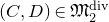 $(C,D) \in \mathfrak{M}_2^{{\rm div}}$
such that
 $\deg D=2$
and the two points of
 $D$
are conjugate. In particular,
 $\mathfrak H$
is a Cartier divisor of
 $\mathfrak{M}_2^{{\rm div}}$
by Proposition 2.17.
For any
 $k \ge 0$
, let
 ${\mathcal H}_k$
be the closed substack of
 $\mathfrak{M}_2^{{\rm div}}$
whose general points are pairs
 $(C,D)$
such that, with
 $F$
denoting the core of
 $C$
,
 $(F,D \cap F) \in \mathfrak H$
and
 $C$
has
 $k$
tails attached to
 $F$
. After
 $(\mathsf r_3\mathsf p_2)$
, let
 \begin{align} \widetilde {\mathfrak{M}}^{{{\rm div}},\mathsf r_3\mathsf p_2}:=\mathfrak{M}_2^{{\rm div}}\times _{\mathfrak{M}_2^{\textrm {wt}}}\widetilde {\mathfrak{M}}^{\mathsf r_3\mathsf p_2},\quad {\mathcal H}_k^{\mathsf r_3\mathsf p_2}:=\textrm {PT}_{\widetilde {\mathfrak{M}}^{{{\rm div}},\mathsf r_3\mathsf p_2}}({\mathcal H}_k),\quad k \ge 0, \end{align}
i.e.
 ${\mathcal H}_k^{\mathsf r_3\mathsf p_2}$
is the proper transform of
 ${\mathcal H}_k$
in
 $\widetilde {\mathfrak{M}}^{{{\rm div}},\mathsf r_3\mathsf p_2}$
for every
 $k \ge 0$
. In
 $(\mathsf r_3\mathsf p_3)$
, we blow up the stack
 $\widetilde {\mathfrak{M}}^{{{\rm div}},\mathsf r_3\mathsf p_2}$
successively along the proper transforms of
 $ {\mathcal H}_k^{\mathsf r_3\mathsf p_2}$
with
 $k \ge 0$
, starting from
 $k=0$
, and obtain
 \begin{align*} \widetilde {\mathfrak{M}}^{{{\rm div}},\mathsf r_3\mathsf p_3} \longrightarrow \widetilde {\mathfrak{M}}^{{{\rm div}},\mathsf r_3\mathsf p_2}.\end{align*}
The stability requirement of
 $\mathfrak{M}_2^{{\rm div}}$
implies that on each connected component of
 $\widetilde {\mathfrak{M}}^{{{\rm div}},\mathsf r_3\mathsf p_2}$
, the process of the sequential blowups
 $(\mathsf r_3\mathsf p_3)$
terminates after finitely many steps.
3.6 The fourth phase of the third round
$(\mathsf r_3\mathsf p_4)$

The process of
 $(\mathsf r_3\mathsf p_4)$
is analogous to the round
 $(\mathsf r_2)$
, but the blowup loci lie in the proper transforms of
 $\mathfrak{M}_2^{{\rm div}}$
instead of
 $\mathfrak{M}_2^{\textrm {wt}}$
.
Notice that the main difference between
 $\overline {\mathfrak{M}}_{(1)}$
and
 $\overline {\mathfrak{M}}_{(5)}^{\mathsf r_1\mathsf p_4}$
in (3.6) is the weight of the core curve. Thus, the exceptional divisors obtained in the phases
 $(\mathsf r_1\mathsf p_1)$
and
 $(\mathsf r_1\mathsf p_5)$
share similar properties. In particular, we define
 \begin{align*} X'_\rho \subset {\mathcal E}_{(5,k)}, \quad \rho =(k,j,\sigma )\in \mathfrak{I}_1, \end{align*}
to be parallel to
 $X_\rho$
in (3.16). For each
 $\rho = (k,j,\sigma ) \in \mathfrak{I}_1$
and every
 $x \in X'_\rho ,$
we denote by
 $F_x$
the core of the underlying curve
 $C_x$
, by
 $q_x$
the node labeled by
 $1$
, and by
 $p_x = \langle {q_x}\rangle$
the pivotal node corresponding to
 $q_x$
. Let
 \begin{align*} {\mathcal Q}_\rho \subset \widetilde {\mathfrak{M}}^{{{\rm div}},\mathsf r_1\mathsf p_5\mathsf s_{k}} := \mathfrak{M}_2^{{\rm div}} \times _{\mathfrak{M}_2^{^{\textrm {wt}}}} \widetilde {\mathfrak{M}}^{\mathsf r_1\mathsf p_5\mathsf s_{k}} ,\quad \rho =(k,j,\sigma )\in \mathfrak{I}_1, \end{align*}
be the closed substack of
 $\widetilde {\mathfrak{M}}^{{{\rm div}},\mathsf r_1\mathsf p_5\mathsf s_{k}}$
whose general points are pairs
 $(x,D)$
satisfying
 \begin{align*} x\in X'_\rho ,\quad \big (F_x,\,(D \cap {F_x})+p_x\big )\in \mathfrak H,\end{align*}
where
 $\mathfrak H$
is as in Section 3.5.
In
 $(\mathsf r_3\mathsf p_4)$
, we blow up
 $\widetilde {\mathfrak{M}}^{{{\rm div}},\mathsf r_3\mathsf p_3}$
successively along the proper transforms of
 \begin{align} {\mathcal Q}_{k,k'}= \bigcup _{\rho \in \mathfrak{I}_1(k,k')} {\mathcal Q}_\rho \ \ \big (\!\subset \widetilde {\mathfrak{M}}^{{{\rm div}},\mathsf r_1\mathsf p_5\mathsf s_{k}}\big ), \quad 1 \le k \le k', \end{align}
with respect to the order inherited from the usual lexicographic order on
 $\mathbb Z \times \mathbb Z$
, and obtain
 \begin{align*} \widetilde {\mathfrak{M}}_2^{{\rm div}}:=\widetilde {\mathfrak{M}}^{{{\rm div}},\mathsf r_3\mathsf p_4} \longrightarrow \widetilde {\mathfrak{M}}^{{{\rm div}},\mathsf r_3\mathsf p_3}.\end{align*}
The stability of
 $\mathfrak{M}_2^{{\rm div}}$
once again implies that on each connected component of
 $\widetilde {\mathfrak{M}}^{{{\rm div}},\mathsf r_3\mathsf p_3}$
,
 $(\mathsf r_3\mathsf p_4)$
terminates after finitely many steps.
3.7 Examples of modular blowups
We conclude Section 3 with a set of examples illustrating the sequential modular blowups.
Example 3.10. We begin with an example that appears simple enough yet still possibly involves all three rounds of blowups.
Let
 $z_0=(C,D) \in \mathfrak{M}^{{\rm div}}_2$
be such that
 $C$
consists of a smooth core
 $F$
and two smooth rational subcurves
 $R_a$
and
 $R_b$
attached to
 $F$
at
 $q_a$
and
 $q_b$
, respectively, and
 $D$
satisfies
 \begin{align*} D\cap R_a=\{\delta _1,\ldots ,\delta _{\ell -1}\},\quad D\cap R_b=\{\delta _\ell ,\ldots ,\delta _m\},\quad D\cap F=\emptyset , \end{align*}
where
 $1 \lt \ell \le m$
. In particular,
 $D\cap R_a$
and
 $D\cap R_b$
are both nonempty. An illustration of
 $C$
is provided in Figure 8, where we follow the convention of Figure 2 by shading the irreducible components of
 $C$
that are positively weighted (i.e. whose intersections with
 $D$
are nonempty). The same convention applies to the remaining figures in Section 3.7.
The curve
 $C$
in Example 3.10.

By Proposition 2.22 (SH1
), locally on a small affine chart
 ${\mathcal V} \longrightarrow \mathfrak{M}^{{\rm div}}_2$
containing the point
 $z_0$
, we have
 \begin{align*}\varphi =\left [\begin{matrix} c_{11} \zeta _a\;\;\;\; & \cdots\;\;\;\; & c_{1,\ell -1} \zeta _a\;\;\;\; & c_{1\ell } \zeta _b\;\;\;\; & \cdots\;\;\;\; & c_{1m} \zeta _b \\ c_{21} \zeta _a\;\;\;\; & \cdots\;\;\;\; & c_{2,\ell -1} \zeta _a\;\;\;\; & c_{2\ell } \zeta _b\;\;\;\; & \cdots\;\;\;\; & c_{2m} \zeta _b \end{matrix} \right ]\!, \end{align*}
where
 $\zeta _a$
and
 $\zeta _b$
are the node-smoothing parameters (i.e. the modular parameters) corresponding to
 $q_a$
and
 $q_b$
, respectively, and
 $c_{ij}$
are invertible functions on
 $\mathcal V$
.
In the above matrix of
 $\varphi$
, the commas in the subscriptions of
 $c_{1,\ell -1}$
and
 $c_{2,\ell -1}$
are only for separation. Hereafter, if necessary, we will use commas to separate the indices in subscriptions should no ambiguity occur.
In
 $(\mathsf r_1\mathsf p_1)$
,
 $\mathcal V$
is blown up along the locus
 $(\zeta _a = \zeta _b=0)$
. After
 $(\mathsf r_1\mathsf p_1)$
, up to switching the symbols
 $a$
and
 $b$
, the pullback
 $\widetilde {\varphi }^{\mathsf r_1\mathsf p_1}$
of
 $\varphi$
locally takes the form
 \begin{align*} \varepsilon \left [\begin{matrix} c_{11}\;\;\;\; & \cdots\;\;\;\; & c_{1,\ell -1}\;\;\;\; & c_{1\ell } \check {\zeta }_b\;\;\;\; & \cdots\;\;\;\; & c_{1m} \check {\zeta }_b \\ c_{21}\;\;\;\; & \cdots\;\;\;\; & c_{2,\ell -1}\;\;\;\; & c_{2\ell } \check {\zeta }_b\;\;\;\; & \cdots\;\;\;\; & c_{2m} \check {\zeta }_b \end{matrix} \right ]\!, \end{align*}
where
 $\varepsilon$
is the local parameter corresponding to the exceptional divisor, and
 $\check {\zeta }_b$
is the proper transform of
 $\zeta _b$
. In other words, up to a multiplicative unit,
 $\zeta _a$
(respectively,
 $\zeta _b$
) pulls back to
 $\varepsilon$
(respectively,
 $\varepsilon \check {\zeta }_b$
).
Recall that
 $\kappa _{ij}$
,
 $1 \le i \lt j \le m$
, are the local parameters on
 $\mathcal V$
whose zero loci consist of
 $z \in {\mathcal V}$
such that
 ${\mathcal D}_i(z)$
and
 ${\mathcal D}_j(z)$
are conjugate points on
 ${\mathcal C}_z$
. By Proposition 2.22 (SH2
), one can apply elementary row and column operations to the above matrix of
 $\widetilde {\varphi }^{\mathsf r_1\mathsf p_1}$
and obtain
 \begin{align*} \varepsilon \left [\begin{matrix} 1\;\;\;\; & 0\;\;\;\; & 0\;\;\;\; & \cdots\;\;\;\; & 0\;\;\;\; & 0\;\;\;\; & 0\;\;\;\; & \cdots\;\;\;\; & 0 \\ 0\;\;\;\; & \check {\kappa }_{12} \cdot \varepsilon\;\;\;\; & \check {\kappa }_{13} \cdot \varepsilon\;\;\;\; & \cdots\;\;\;\; & \check {\kappa }_{1,\ell -1} \cdot \varepsilon\;\;\;\; & \check {\kappa }_{1\ell } \cdot \check {\zeta }_b\;\;\;\; & \check {\kappa }_{\ell ,\ell+1} \cdot \varepsilon \cdot \check {\zeta }_b^2\;\;\;\; & \cdots\;\;\;\; & \check {\kappa }_{\ell m} \cdot \varepsilon \cdot \check {\zeta }_b^2 \end{matrix} \right ]\!, \end{align*}
where
 $\check {\kappa }_{ij}$
refers to the proper transform of
 $\kappa _{ij}$
, which is equivalent to its pullback in this case. Notice that, depending on the value of
 $\ell$
and
 $m$
, some columns above may not exist.
Below, we analyze
 $\widetilde {\varphi }^{\mathsf r_1\mathsf p_1}$
depending on the location of
 $q_a$
and
 $q_b$
on the core
 $F$
of
 $C$
.
Case (A):
 $q_a$
is in general position. This means
 $q_a$
is neither Weierstrass nor conjugate to
 $q_b$
. Hence
 $\kappa _{1i}$
with
 $2 \le i \le \ell$
are all invertible and so are their pullbacks. Therefore, the matrix of
 $\widetilde {\varphi }^{\mathsf r_1\mathsf p_1}$
, after further elementary column operations, can be rewritten as
 \begin{align*} \varepsilon \left [\begin{matrix} 1\;\;\;\; & 0\;\;\;\; & 0\;\;\;\; & \cdots\;\;\;\; & 0\;\;\;\; & 0\;\;\;\; & 0\;\;\;\; & \cdots\;\;\;\; & 0 \\ 0\;\;\;\; & \varepsilon\;\;\;\; & 0\;\;\;\; & \cdots\;\;\;\; & 0\;\;\;\; & \check {\zeta }_b\;\;\;\; & 0\;\;\;\; & \cdots\;\;\;\; & 0 \end{matrix} \right ]\!. \end{align*}
If
 $\ell=2$
(i.e.
 $|D \cap R_a| = 1$
), then the second column
 $[0,\varepsilon ]^T$
does not exist and the matrix is already diagonalized.
If
 $\ell \ge 3$
(i.e.
 $|D \cap R_a| \ge 2$
), we observe that the remaining phases of
 $(\mathsf r_1)$
do not affect this chart, and the blowups in
 $(\mathsf r_2)$
that may affect this chart have the center
 $X_{2,2}$
(cf. Figure 2), which locally is given by
 $(\varepsilon = \check {\zeta }_b=0)$
. Therefore, after
 $(\mathsf r_2)$
, the pullback
 $\widetilde {\varphi }^{\mathsf r_2}$
of
 $\varphi$
becomes diagonalized.
Case (B):
 $q_a$
and
 $q_b$
are a pair of conjugate points on the core
 $F$
. Since
 $F$
is smooth, neither
 $q_a$
nor
 $q_b$
is a Weierstrass point of
 $F$
, because of Lemma 2.14. Lemma 2.20 then implies that
 $\kappa _{1i}$
with
 $2 \le i \le \ell - 1$
and
 $\kappa _{\ell k}$
with
 $\ell+1 \le k \le m$
are all invertible and so are their proper transforms. Therefore, the matrix of
 $\widetilde {\varphi }^{\mathsf r_1\mathsf p_1}$
, after further elementary column operations, can be rewritten as
 \begin{align*} \varepsilon \left [\begin{matrix} 1\;\;\;\; & 0\;\;\;\; & 0\;\;\;\; & \cdots\;\;\;\; & 0\;\;\;\; & 0\;\;\;\; & 0\;\;\;\; & 0\;\;\;\; & \cdots\;\;\;\; & 0 \\ 0\;\;\;\; & \varepsilon\;\;\;\; & 0\;\;\;\; & \cdots\;\;\;\; & 0\;\;\;\; & \check {\kappa }_{1\ell }\check {\zeta }_b\;\;\;\; & \varepsilon \check {\zeta }_b^2\;\;\;\; & 0\;\;\;\; & \cdots\;\;\;\; & 0 \end{matrix} \right ]\!. \end{align*}
If
 $\ell = m=2$
(i.e.
 $|D \cap R_a| = |D \cap R_b| = 1$
), then only the first and the
 $\ell$
th columns exist, and the matrix takes the form
 \begin{align*} \left [\begin{matrix} 1\;\;\;\; & 0 \\ 0\;\;\;\; & \check {\kappa }_{1\ell } \check {\zeta }_b \end{matrix} \right ]\!, \end{align*}
which is already diagonalized.
If
 $2 = \ell \lt m$
(i.e.
 $1 = |D \cap R_a| \lt |D \cap R_b|$
), then the second column
 $[0,\varepsilon ]^T$
does not exist and the matrix takes the form
 \begin{align*} \left [\begin{matrix} \varepsilon\;\;\;\; & 0\\ 0\;\;\;\; & \varepsilon \check {\zeta }_b \end{matrix}\right ] \left [\begin{matrix} 1\;\;\;\; & 0\;\;\;\; & 0\;\;\;\; & 0\;\;\;\; & \cdots\;\;\;\; & 0 \\ 0\;\;\;\; & \check {\kappa }_{1\ell }\;\;\;\; & \varepsilon \check {\zeta }_b\;\;\;\; & 0\;\;\;\; & \cdots\;\;\;\; & 0 \end{matrix} \right ]\!. \end{align*}
The blowups in
 $(\mathsf r_1\mathsf p_2)$
to
 $(\mathsf r_1\mathsf p_4)$
do not affect the chart. In
 $(\mathsf r_1\mathsf p_5)$
, the locus
 $(\check {\zeta }_b=0)$
is blown up, which does not yield anything new because the blowup center is a smooth Cartier divisor. The blowups in
 $(\mathsf r_2)$
,
 $(\mathsf r_3\mathsf p_2)$
and
 $(\mathsf r_3\mathsf p_3)$
do not affect the chart either, whereas in
 $(\mathsf r_3\mathsf p_1)$
and
 $(\mathsf r_3\mathsf p_4)$
, the blowup centers are locally given by
 \begin{align*}(\check {\kappa }_{1\ell }=\varepsilon=0)\quad \textrm {and}\quad (\check {\kappa }_{1\ell }=\check {\zeta }_b=0), \end{align*}
respectively. It is easy to check that after
 $(\mathsf r_3\mathsf p_4)$
, the pullback
 $\widetilde {\varphi }^{\mathsf r_3\mathsf p_4}$
of
 $\varphi$
becomes diagonalized.
If
 $\ell \ge 3$
(i.e.
 $|D \cap R_a| \ge 2$
), then the second column
 $[0,\varepsilon ]^T$
exists and the matrix of
 $\varphi ^{\mathsf r_1\mathsf p_1}$
, after another column addition, takes the form
 \begin{align*} \varepsilon \left [\begin{matrix} 1\;\;\;\; & 0\;\;\;\; & 0\;\;\;\; & \cdots\;\;\;\; & 0\;\;\;\; & 0\;\;\;\; & 0\;\;\;\; & \cdots\;\;\;\; & 0 \\ 0\;\;\;\; & \varepsilon\;\;\;\; & 0\;\;\;\; & \cdots\;\;\;\; & 0\;\;\;\; & \check {\kappa }_{1\ell }\check {\zeta }_b\;\;\;\; & 0\;\;\;\; & \cdots\;\;\;\; & 0 \end{matrix} \right ]\!. \end{align*}
The blowups in
 $(\mathsf r_1\mathsf p_2)$
to
 $(\mathsf r_1\mathsf p_5)$
and
 $(\mathsf r_3\mathsf p_2)$
to
 $(\mathsf r_3\mathsf p_4)$
do not affect (the pullback of) the chart. In
 $(\mathsf r_2)$
and
 $(\mathsf r_3\mathsf p_1)$
, the blowup centers are locally given by
 \begin{align*}(\varepsilon = \check {\zeta }_b=0)\quad \textrm {and}\quad \textrm {PT}(\varepsilon =\check {\kappa }_{1\ell }= 0), \end{align*}
respectively, where
 $\textrm {PT}$
refers to the proper transform. So after
 $(\mathsf r_3\mathsf p_1)$
, the pullback
 $\widetilde {\varphi }^{\mathsf r_3\mathsf p_1}$
of
 $\varphi$
becomes diagonalized.
Case (C):
 $q_a$
is a Weierstrass point on the core
 $F$
. Since
 $F$
is smooth,
 $q_a$
and
 $q_b$
cannot be conjugate, by Lemma 2.14, and hence
 $\kappa _{1 k}$
,
 $\ell \le k \le m$
, are all invertible and so are their proper transforms. Taking Proposition 2.22 (SH3
) into consideration, we see that the matrix of
 $\widetilde {\varphi }^{\mathsf r_1\mathsf p_1}$
, after further elementary column operations, can be rewritten as
 \begin{align*} \varepsilon \left [\begin{matrix} 1\;\;\;\; & 0\;\;\;\; & 0\;\;\;\; & 0\;\;\;\; & \cdots\;\;\;\; & 0\;\;\;\; & 0\;\;\;\; & 0\;\;\;\; & \cdots\;\;\;\; & 0 \\ 0\;\;\;\; & \check {\kappa }_{12}\varepsilon\;\;\;\; & \varepsilon^2\;\;\;\; & 0\;\;\;\; & \cdots\;\;\;\; & 0\;\;\;\; & \check {\zeta }_b\;\;\;\; & 0\;\;\;\; & \cdots\;\;\;\; & 0 \end{matrix} \right ]\!. \end{align*}
If
 $\ell=2$
(i.e.
 $|D \cap R_a| = 1$
), then the second and third columns
 $[0,\check {\kappa }_{12}\varepsilon ]^T$
and
 $[0,\varepsilon^2]^T$
do not exist, so the matrix is already diagonalized.
If
 $\ell \ge 3$
(i.e.
 $|D \cap R_a| \ge 2$
), notice that the blowups in
 $(\mathsf r_1\mathsf p_2)$
to
 $(\mathsf r_1\mathsf p_5)$
and
 $(\mathsf r_3\mathsf p_3)$
to
 $(\mathsf r_3\mathsf p_4)$
do not affect (the pullback of) the chart. The blowups in
 $(\mathsf r_2)$
may affect the chart only when
 $\check {\zeta }_b$
is not invertible (otherwise the matrix is already diagonalized), in which case the relevant blowup center is
 $(\varepsilon = \check {\zeta }_b=0)$
. After
 $(\mathsf r_2)$
, on the new chart given by
 $\check {\zeta }_b = \varepsilon '$
and
 $\varepsilon = \varepsilon '\check {\varepsilon }$
(where
 $\varepsilon ' = 0$
defines the exceptional divisor obtained in
 $(\mathsf r_2)$
), the matrix becomes diagonalized. On the new chart given by
 $\varepsilon = \varepsilon '$
and
 $\check {\zeta }_b = \varepsilon '\check {\zeta }_b'$
, the matrix can be written as
 \begin{align*} \left [\begin{matrix} \varepsilon '\;\;\;\; & 0\\ 0\;\;\;\; & (\varepsilon ')^2 \end{matrix}\right ] \left [\begin{matrix} 1\;\;\;\; & 0\;\;\;\; & 0\;\;\;\; & 0\;\;\;\; & \cdots\;\;\;\; & 0\;\;\;\; & 0\;\;\;\; & 0\;\;\;\; & \cdots\;\;\;\; & 0 \\ 0\;\;\;\; & \check {\kappa }_{12}\;\;\;\; & \varepsilon'\;\;\;\; & 0\;\;\;\; & \cdots\;\;\;\; & 0\;\;\;\; & \check {\zeta }_b'\;\;\;\; & 0\;\;\;\; & \cdots\;\;\;\; & 0 \end{matrix} \right ]\!. \end{align*}
We remark that the third column
 $[0,\varepsilon ']^T$
of the right-hand matrix above does not exist if
 $\ell=3$
(i.e.
 $|D \cap R_a| = 2$
).
The blowups in
 $(\mathsf r_3\mathsf p_1)$
do not affect this new chart locally. In
 $(\mathsf r_3\mathsf p_2)$
(and
 $(\mathsf r_3\mathsf p_3)$
if
 $\ell=3$
), the blowup center is locally given by
 \begin{align*}(\check {\kappa }_{12}=\varepsilon '= \check {\zeta }_b'=0)\quad \big (\textrm {and}\quad \textrm {PT}(\check {\kappa }_{12}=\check {\zeta }_b'= 0)\quad \textrm {if}\quad\,\ell=3\big ), \end{align*}
where
 $\textrm {PT}$
refers to the proper transform. So after
 $(\mathsf r_3\mathsf p_2)$
 $\big ((\mathsf r_3\mathsf p_3)$
if
 $\ell=3\big )$
, the pullback of
 $\varphi$
becomes diagonalized.
Example 3.11. Let
 $z_0=(C,D)$
, where
 $C$
is made of a smooth core curve
 $F$
with weight zero and two smooth rational tails
 $T_1$
and
 $T_2$
with positive weights, attached to
 $F$
at
 $q_a$
and
 $q_b$
, respectively. Further, let
 $T_1$
be made of a single smooth rational curve
 $R_a$
, and
 $T_2$
be made of three rational curves
 $R_b,$
 $R_c$
and
 $R_d$
such that
 $R_b$
is attached to
 $F$
and
 $R_c$
and
 $R_d$
are attached to
 $R_b$
at two distinct points
 $q_c$
and
 $q_d$
, respectively; see Figure 9.
We assume that
 $q_a$
and
 $q_b$
are in general positions on
 $F$
. In other words, they are not conjugate points, and neither is Weierstrass.
By Proposition 2.22 (SH1
), locally on some affine chart
 $\mathcal V$
containing the point
 $z_0$
, we have
 \begin{align*}\varphi =\left [\begin{matrix} a_{11} \zeta _a\;\;\;\; & c_{11} \zeta _b\zeta _c\;\;\;\; & d_{11} \zeta _b\zeta _d\;\;\;\; & \cdots \\ a_{21} \zeta _a\;\;\;\; & c_{21} \zeta _b\zeta _c\;\;\;\; & d_{21} \zeta _b\zeta _d\;\;\;\; & \cdots \\ \end{matrix} \right ]\!, \end{align*}
where
 $\zeta _a$
(respectively,
 $\zeta _b, \zeta _c, \zeta _d$
) is the node-smoothing parameter for
 $q_a$
(respectively,
 $q_b,$
 $q_c,$
 $q_d$
), and
 $a_{ij}$
,
 $c_{ij}$
and
 $d_{ij}$
are invertible functions on
 $\mathcal V$
. Each of the omitted entries can also be divided by
 $\zeta _a$
,
 $\zeta _b\zeta _c$
, or
 $\zeta _b\zeta _d$
. Moreover, by Proposition 2.22 (SH2
), the vanishing orders of
 $2 \times 2$
minors of
 $\varphi$
can be higher: under the assumption of this example, we have
 \begin{align*} \det \left [\begin{matrix} a_{11}\;\;\;\; & c_{11}\\ a_{21}\;\;\;\; & c_{21} \end{matrix}\right ]\!,\, \det \left [\begin{matrix} a_{11}\;\;\;\; & d_{11}\\ a_{21}\;\;\;\; & d_{21} \end{matrix}\right ] \in \Gamma ({\mathscr O}_{\mathcal V}^*),\quad \det \left [\begin{matrix} c_{11}\;\;\;\; & d_{11}\\ c_{21}\;\;\;\; & d_{21} \end{matrix}\right ]\Big /\zeta _{b} \in \Gamma ({\mathscr O}_{\mathcal V}^*) . \end{align*}
In addition, if
 $ R_a$
has weight greater than one, the
 $2 \times 2$
minors corresponding to the points of
 $D \cap R_a$
may need to be taken into consideration, and these contain
 $\zeta _a^2$
as a factor. Similarly, the term
 $\zeta _b^2\zeta _c^2$
(respectively,
 $\zeta _b^2\zeta _d^2$
) may need to be taken into consideration if
 $R_c$
(respectively,
 $R_d$
) has weight greater than one.
The curve
 $C$
in Example 3.11.

Here, we point out the following. In
 $(\mathsf r_1\mathsf p_1)$
, for any
 $z_0=(C,{\bf w}) \in \mathfrak{M}_2^{\textrm {wt}}$
whose core is of weight 0, the farther the separating nodes are away from the core, the later the corresponding parameters appear in the local equations of (the proper transforms of) the blowup centers. For instance, in the above example, for the nodes
 $q_a$
and
 $q_b$
that are closest to the core, locally at
 $z_0$
,
 \begin{align*}(\zeta _a=\zeta _b=0)\end{align*}
defines the first blowup center
 $\overline {\mathfrak{M}}_{(1,2)} \cap {\mathcal V}$
. After this blowup, on the chart given by
 $\zeta _b = \varepsilon _b$
and
 $\zeta _a = \varepsilon _b\check {\zeta }_a$
, the locus
 \begin{align*}(\check {\zeta }_a= \zeta _c=\zeta _d=0)\end{align*}
locally defines the next blowup center, the proper transform of
 $\overline {\mathfrak{M}}_{(1,3)}$
. This generalizes to all separating nodes that are farther from the core, if any.
Going back to the current example, the rooted tree of this example is identical to that of [Reference Hu and LiHL10, Example 5.17]. The calculation within each phase of
 $(\mathsf r_1)$
is also similar to [Reference Hu and LiHL10].
More precisely, assume that
 $R_a$
,
 $R_c$
and
 $R_d$
all have weight one. Then, using similar calculations to those of [Reference Hu and LiHL10, Example 5.17] and then applying Proposition 2.22, one finds that after
 $(\mathsf r_1)$
, up to switching the symbols
 $c$
and
 $d$
, the pullback
 $\widetilde {\varphi }^{\mathsf r_1}$
of
 $\varphi$
may take one of the following forms:
 \begin{align*} & \left [\begin{matrix} \varepsilon _a^{\mathsf r_1\mathsf p_1}\;\;\;\; & 0\\ 0\;\;\;\; & \varepsilon _a^{\mathsf r_1\mathsf p_1}\varepsilon _b^{\mathsf r_1\mathsf p_5}\varepsilon _c^{\mathsf r_1\mathsf p_5} \end{matrix}\right ] \left [\begin{matrix} 1\;\;\;\; & 0\;\;\;\; & 0 \\ 0\;\;\;\; & 1\;\;\;\; & \check {\zeta }_d \\ \end{matrix} \right ]\!,\ \ & & \left [\begin{matrix} \varepsilon _a^{\mathsf r_1\mathsf p_1}\;\;\;\; & 0\\ 0\;\;\;\; & \varepsilon _a^{\mathsf r_1\mathsf p_1}\varepsilon _c^{\mathsf r_1\mathsf p_5} \end{matrix}\right ] \left [\begin{matrix} 1\;\;\;\; & 0\;\;\;\; & 0 \\ 0\;\;\;\; & 1\;\;\;\; & \check {\zeta }_d \\ \end{matrix} \right ]\!, \\ & \left [\begin{matrix} \varepsilon _b^{\mathsf r_1\mathsf p_1}\varepsilon _a^{\mathsf r_1\mathsf p_1}\;\;\;\; & 0\\ 0\;\;\;\; & \varepsilon _b^{\mathsf r_1\mathsf p_1}\varepsilon _a^{\mathsf r_1\mathsf p_1}\varepsilon _c^{\mathsf r_1\mathsf p_5} \end{matrix}\right ] \left [\begin{matrix} 1\;\;\;\; & 0\;\;\;\; & 0 \\ 0\;\;\;\; & 1\;\;\;\; & \check {\zeta }_d \\ \end{matrix} \right ]\!, & & \varepsilon _b^{\mathsf r_1\mathsf p_1} \varepsilon _c ^{\mathsf r_1\mathsf p_1} \left [\begin{matrix} 0\;\;\;\; & 1\;\;\;\; & 0 \\ 1\;\;\;\; & 0\;\;\;\; & \varepsilon _b^{\mathsf r_1\mathsf p_1}\check {\zeta }_d \end{matrix} \right ]\!, \\ & \varepsilon _b^{\mathsf r_1\mathsf p_1} \varepsilon _c ^{\mathsf r_1\mathsf p_1} \left [\begin{matrix} 0\;\;\;\; & 1\;\;\;\; & 0 \\ \check {\zeta }_a\;\;\;\; & 0\;\;\;\; & \varepsilon _b^{\mathsf r_1\mathsf p_1} \end{matrix} \right ]\!, & & \left [ \begin{matrix} \varepsilon _b^{\mathsf r_1\mathsf p_1} \varepsilon _c ^{\mathsf r_1\mathsf p_1}\;\;\;\; & 0\\ 0\;\;\;\; & \varepsilon _b^{\mathsf r_1\mathsf p_1} \varepsilon _c ^{\mathsf r_1\mathsf p_1}\varepsilon _a^{\mathsf r_1\mathsf p_5} \end{matrix} \right ] \left [\begin{matrix} 0\;\;\;\; & 1\;\;\;\; & 0 \\ 1\;\;\;\; & 0\;\;\;\; & \varepsilon _b^{\mathsf r_1\mathsf p_1}\check {\zeta }_d \end{matrix} \right ]\!, \\ & \textrm {or}\quad \left [ \begin{matrix} \varepsilon _b^{\mathsf r_1\mathsf p_1} \varepsilon _c ^{\mathsf r_1\mathsf p_1}\;\;\;\; & 0\\ 0\;\;\;\; & \varepsilon _b^{\mathsf r_1\mathsf p_1} \varepsilon _c ^{\mathsf r_1\mathsf p_1}\varepsilon _d^{\mathsf r_1\mathsf p_5} \end{matrix} \right ] \left [\begin{matrix} 0\;\;\;\; & 1\;\;\;\; & 0 \\ \check {\zeta }_a\;\;\;\; & 0\;\;\;\; & \varepsilon _b^{\mathsf r_1\mathsf p_1} \end{matrix} \right ]\!, & & \end{align*}
where the
 $\varepsilon$
are local parameters corresponding to the proper transforms of the exceptional divisors, the superscripts of
 $\varepsilon$
indicate the corresponding phases in (
 $\mathsf r_1$
), and
 $\check {\zeta }_a$
and
 $\check {\zeta }_d$
are proper transforms of
 $\zeta _a$
and
 $\zeta _d$
, respectively. Among the above seven possibilities of
 $\widetilde {\varphi }^{\mathsf r_1}$
, five are already diagonalized; in either of the remaining two cases, the only blowup center of (
 $\mathsf r_2$
) that may affect
 $\widetilde {\varphi }^{\mathsf r_1}$
is locally defined by
 \begin{align*} \big (\varepsilon _b^{\mathsf r_1\mathsf p_1}=\check {\zeta }_a=0\big ), \end{align*}
and hence the pullback of
 $\varphi$
after (
 $\mathsf r_2$
) becomes diagonalized.
Next, consider the case when at least one of
 $R_a$
,
 $R_b$
and
 $R_c$
, say
 $R_a$
, has weight greater than one. In such a case, by Proposition 2.22 (SH2
), entries containing
 $\zeta _a^2$
may occur in
 $\varphi$
. For instance, one finds that after
 $(\mathsf r_1\mathsf p_1)$
(hence after
 $(\mathsf r_1)$
), on the chart given by
 $\zeta _a = \varepsilon _a$
and
 $\zeta _b = \varepsilon _a\check {\zeta }_b$
, the pullback of
 $\varphi$
takes the following form:
 \begin{align*}\varepsilon _a \left [\begin{matrix} 1\;\;\;\; & 0\;\;\;\; & 0\;\;\;\; & 0\;\;\;\; & 0\;\;\;\; & \cdots \\ 0\;\;\;\; & \varepsilon _a\;\;\;\; & \check {\zeta }_b \zeta _c\;\;\;\; & \check {\zeta }_b \zeta _d\;\;\;\; & 0\;\;\;\; & \cdots \\ \end{matrix} \right ]\!.\end{align*}
The blowup in (
 $\mathsf r_2$
) that may affect this chart has the centers locally defined by
 \begin{align} (\varepsilon _a=\check {\zeta }_b=0)\quad \textrm {and}\quad \textrm {PT}(\varepsilon _a=\zeta _c=\zeta _d=0), \end{align}
where
 $\textrm {PT}$
refers to the proper transform. Globally the two loci correspond to
 $X_{2,2}$
and
 $X_{2,3}$
, respectively; see Figure 2. (The derived tree in this case is labeled (3) in Figure 18.) Then, following similar calculations as in
 $(\mathsf r_1)$
, one finds that after
 $(\mathsf r_2)$
, the pullback of
 $\varphi$
becomes diagonalized.
Similarly, one finds that after
 $(\mathsf r_2)$
, the pullback of
 $\varphi$
becomes diagonalized on other charts.
Example 3.12. Let
 $z_0=(C,D)$
be the same as in Example 3.11 but with one difference:
 ${\rm we\,\ assume\,\ that}$
 $q_a$
 ${\rm is\,\ a\,\ Weierstrass\,\ point\,\ of\,\ the\,\ core}$
 $F$
 ${\rm of}$
 $C$
. Since
 $F$
is assumed to be smooth,
 $q_a$
and
 $q_b$
cannot be conjugate. We further assume that
 $D \cap R_a = \{\delta _1,\ldots ,\delta _{k}\}$
with
 $k \ge 3$
.
After
 $(\mathsf r_1)$
, on the chart given by
 $\zeta _a = \varepsilon _a$
and
 $\zeta _b = \varepsilon _a\check {\zeta }_b$
, the pullback of
 $\varphi$
takes the following form:
 \begin{align*}\varepsilon _a \left [\begin{matrix} 1\;\;\;\; & 0\;\;\;\; & 0\;\;\;\; & 0\;\;\;\; & 0\;\;\;\; & 0\;\;\;\; & \cdots \\ 0\;\;\;\; & \check {\kappa }_{12}\varepsilon _a\;\;\;\; & \varepsilon _a^2\;\;\;\; & \check {\zeta }_b \zeta _c\;\;\;\; & \check {\zeta }_b \zeta _d\;\;\;\; & 0\;\;\;\; & \cdots \\ \end{matrix} \right ]\!,\end{align*}
where
 $\check {\kappa }_{12}$
is the proper transform of
 $\kappa _{12}$
as in Example 3.10. The blowup in (
 $\mathsf r_2$
) that may affect this chart still has the centers locally defined by
 \begin{align*} (\varepsilon _a=\check {\zeta }_b=0)\quad \textrm {and}\quad \textrm {PT}(\varepsilon _a=\zeta _c=\zeta _d=0). \end{align*}
Following similar calculations as in Examples 3.10 and 3.11, one finds that after
 $(\mathsf r_2)$
, on the new chart given by
 $\varepsilon _a = \varepsilon '$
and
 $\check {\zeta }_b = \varepsilon '\check {\zeta }_b'$
, the pullback of
 $\varphi$
takes the form
 \begin{align*} \left [\begin{matrix} \varepsilon '\;\;\;\; & 0\\ 0\;\;\;\; & (\varepsilon ')^2 \end{matrix}\right ] \left [\begin{matrix} 1\;\;\;\; & 0\;\;\;\; & 0\;\;\;\; & 0\;\;\;\; & 0\;\;\;\; & 0\;\;\;\; & \cdots \\ 0\;\;\;\; & \check {\kappa }_{12}\;\;\;\; & \varepsilon '\;\;\;\; & \check {\zeta }_b' \zeta _c\;\;\;\; & \check {\zeta }_b' \zeta _d\;\;\;\; & 0\;\;\;\; & \cdots \\ \end{matrix} \right ]\!.\end{align*}
The blowup in (
 $\mathsf r_3\mathsf p_2$
) that may affect this chart has the centers locally defined by
 \begin{align} (\check {\kappa }_{12}=\varepsilon '=\check {\zeta }_b'=0)\quad \textrm {and}\quad \textrm {PT}(\check {\kappa }_{12}=\varepsilon '=\zeta _c=\zeta _d=0). \end{align}
Therefore, after
 $(\mathsf r_3\mathsf p_2)$
, the pullback of
 $\varphi$
becomes diagonalized.
Example 3.13. Let
 $z_0=(C,D)$
be the same as in Example 3.11 but with one difference:
 ${\rm we\,assume\,that}$
 $q_a$
 ${\rm and}$
 $q_b$
 ${\rm are\,\ conjugate\,\ points\,\ on\,\ the\,\ core}$
 $F$
 ${\rm of}$
 $C$
. Since
 $F$
is assumed to be smooth, neither
 $q_a$
nor
 $q_b$
is Weierstrass. We further assume that
 $|D \cap R_\bullet | \ge 3$
for
 $\bullet = a,c,d$
. Moreover, we assume that
 $\delta _1 \in R_a$
,
 $\delta _2 \in R_b$
and
 $\delta _3 \in R_c$
.
After
 $(\mathsf r_1)$
, on the chart given by
 \begin{align*}\zeta _a=\varepsilon _1\varepsilon _2,\quad \zeta _b=\varepsilon _1,\quad \zeta _c=\varepsilon _1\varepsilon _2\check {\zeta }_c,\quad \textrm {and}\quad \zeta _d=\varepsilon _1\varepsilon _2\check {\zeta }_d, \end{align*}
(i.e. locally one first blows up along
 $(\zeta _a = \zeta _b=0)$
, then on the chart given by
 $\zeta _b = \varepsilon _1$
and
 $\zeta _a = \varepsilon _1\check {\zeta }_a$
, one blows up along
 $(\check {\zeta }_a = \zeta _c = \zeta _d=0)$
and considers the new chart given by
 $\check {\zeta }_a = \varepsilon _2$
,
 $\zeta _c = \varepsilon _2\check {\zeta }_c$
and
 $\zeta _d = \varepsilon _2\check {\zeta }_d$
,) the pullback of
 $\varphi$
takes the following form:
 \begin{align} \varepsilon _1\varepsilon _2 \left [\begin{matrix} 1\;\;\;\; & 0\;\;\;\; & 0\;\;\;\; & 0\;\;\;\; & 0\;\;\;\; & \cdots \\ 0\;\;\;\; & \varepsilon _1\varepsilon _2\;\;\;\; & \check {\kappa }_{12}\check {\zeta }_c\;\;\;\; & \check {\kappa }_{13}\check {\zeta }_d\;\;\;\; & 0\;\;\;\; & \cdots \\ \end{matrix} \right ]\!, \end{align}
where
 $\check {\kappa }_{ij}$
is the pullback of
 $\kappa _{ij}$
as in Example 3.10. Proposition 2.22 (SH3
) implies that
 \begin{align*} \kappa _{13}=f'\kappa _{12}+g'\zeta _b, \quad \Longrightarrow \quad \check {\kappa }_{13}=f\check {\kappa }_{12}+g\varepsilon _1, \end{align*}
where
 $f'$
,
 $g'$
,
 $f$
and
 $g$
are some units.
The blowup in (
 $\mathsf r_2$
) that may affect this chart still has the centers locally defined by
 \begin{align*} (\varepsilon _2=\check {\zeta }_c=\check {\zeta }_d=0)\quad \textrm {and}\quad \textrm {PT}(\varepsilon _1=\check {\zeta }_c=\check {\zeta }_d=0). \end{align*}
Globally, these two loci correspond to the substacks
 $X_{3,3}$
and
 $X_{2,3}$
of
 $\widetilde {\mathfrak{M}}^{\mathsf r_2}$
; see (3.17) for the notation and Figure 2 for an illustration. (The derived tree in this case is labeled (1) in Figure 18.)
Following the order (3.18), we first blow up along
 $(\varepsilon _2=\check {\zeta }_c=\check {\zeta }_d=0)$
.
On the chart given by
 $\varepsilon _2 = \varepsilon '$
,
 $\check {\zeta }_c = \varepsilon '\check {\zeta }_c'$
and
 $\check {\zeta }_d = \varepsilon '\check {\zeta }_d'$
, the second row of the pullback of
 $\varphi$
can be rewritten as
 \begin{align*} \varepsilon _1(\varepsilon ')^2\big [\ 0\ \ \ \varepsilon _1\ \ \ \check {\kappa }_{12}\check {\zeta }_c'\ \ \ \check {\kappa }_{13}\check {\zeta }_d'\ \ \ \cdots \ \big ] \ =\ \varepsilon _1(\varepsilon ')^2\big [\ 0\ \ \ \varepsilon _1\ \ \ \check {\kappa }_{12}\check {\zeta }_c'\ \ \ (f\check {\kappa }_{12}+g\varepsilon _1)\check {\zeta }_d'\ \ \ \cdots \ \big ]. \end{align*}
The remaining blowups in
 $(\mathsf r_2)$
, as well as those in
 $(\mathsf r_3\mathsf p_1)$
, that may affect this chart have centers locally given by
 \begin{align*} \textrm {PT}(\varepsilon _1=\check {\zeta }_c=\check {\zeta }_d=0)=(\varepsilon _1=\check {\zeta }_c'=\check {\zeta }_d'=0)\quad \textrm {and}\quad \textrm {PT}(\varepsilon _1=\check {\kappa }_{12}=0), \end{align*}
respectively. Therefore, the pullback of
 $\varphi$
is diagonalized after
 $(\mathsf r_3\mathsf p_1)$
.
On the chart given by
 $\check {\zeta }_c = \varepsilon '$
,
 $\varepsilon _2 = \varepsilon '\check {\varepsilon }_2$
and
 $\check {\zeta }_d = \varepsilon '\check {\zeta }_d'$
, the second row of the pullback of
 $\varphi$
can be rewritten as
 \begin{align*} \varepsilon _1(\varepsilon ')^2\big [\ 0\ \ \ \varepsilon _1\check {\varepsilon }_2\ \ \ \check {\kappa }_{12}\ \ \ \check {\kappa }_{13}\check {\zeta }_d'\ \ \ \cdots \ \big ] \ =\ \varepsilon _1(\varepsilon ')^2\big [\ 0\ \ \ \varepsilon _1\check {\varepsilon }_2\ \ \ \check {\kappa }_{12}\ \ \ \varepsilon _1\check {\zeta }_d'\ \ \ \cdots \ \big ]. \end{align*}
The proper transform of
 $(\varepsilon _1=\check {\zeta }_c=\check {\zeta }_d=0)$
does not affect this chart, whereas the relevant blowup centers in
 $(\mathsf r_3\mathsf p_1)$
are
 \begin{align*} (\check {\varepsilon }_2=\check {\zeta }_d'=\check {\kappa }_{12}= 0)\quad \textrm {and}\quad \textrm {PT}(\varepsilon _1=\check {\kappa }_{12}=0), \end{align*}
respectively. Therefore, the pullback of
 $\varphi$
is diagonalized after
 $(\mathsf r_3\mathsf p_1)$
.
The argument on the chart given by
 $\check {\zeta }_d = \varepsilon '$
,
 $\varepsilon _2 = \varepsilon '\check {\varepsilon }_2$
and
 $\check {\zeta }_c = \varepsilon '\check {\zeta }_c'$
is parallel.
At the end of this example, we remark that in
 $(\mathsf r_2)$
, if the order (3.18) were replaced by the usual lexicographic order on
 $\mathbb Z \times \mathbb Z$
, then after the entire three rounds of blowups terminate, the pullback of
 $\varphi$
would fail to be diagonalizable on some chart. To see this, we blow up
 $X_{2,3}$
prior to
 $X_{3,3}$
in this example. Locally, this means that the locus
 $(\varepsilon _1 = \check {\zeta }_c = \check {\zeta }_d=0)$
is blown up before
 $(\varepsilon _2 = \check {\zeta }_c = \check {\zeta }_d=0)$
. Then, on the chart given by
 $\varepsilon _1 = \varepsilon '$
,
 $\check {\zeta }_c = \varepsilon '\check {\zeta }_c'$
and
 $\check {\zeta }_d = \varepsilon '\check {\zeta }_d'$
, the second row of the pullback of (3.30) can be rewritten as
 \begin{align*} \varepsilon _2(\varepsilon ')^2\big [\ 0\ \ \ \varepsilon _2\ \ \ \check {\kappa }_{12}\check {\zeta }_c'\ \ \ (f\check {\kappa }_{12}+g\varepsilon ')\check {\zeta }_d'\ \ \ \cdots \ \big ]. \end{align*}
After blowing up
 $\textrm {PT}(\varepsilon _2 = \check {\zeta }_c = \check {\zeta }_d=0)= (\varepsilon _2 = \check {\zeta }_c' = \check {\zeta }_d' = 0)$
, on the chart given by
 $\check {\zeta }_c' = \varepsilon ''$
,
 $\varepsilon _2 = \varepsilon ''\check {\varepsilon }_2$
and
 $ \check {\zeta }_d' = \varepsilon ''\check {\zeta }_d''$
, the second row of the pullback of
 $\varphi$
can be further rewritten as
 \begin{align*} \varepsilon _2(\varepsilon '\varepsilon '')^2\big [\ 0\ \ \ \check {\varepsilon }_2\ \ \ \check {\kappa }_{12}\ \ \ \varepsilon '\check {\zeta }_d''\ \ \ \cdots \ \big ]. \end{align*}
The problem is that the locus
 $(\check {\varepsilon }_2 = \varepsilon ' = \check {\kappa }_{12} = 0)$
, which must be blown up so as to simplify the matrix above, does not correspond to any blowup center in
 $(\mathsf r_3)$
. Indeed, such loci lie deeply in the intersections of the exceptional divisors from the previous steps, so it seems formidable to organize them in a systematic way should such blowups be included. However, by introducing the order (3.18) in
 $(\mathsf r_2)$
, such issues can be avoided nicely.
Example 3.14. Let
 $z_0 = (C,D) \in \mathfrak{M}_2^{\textrm {div}}$
be such that the core
 $F$
of
 $C$
is comprised of a smooth rational subcurve
 $B$
and a smooth genus 1 subcurve
 $C_2$
, meeting at two points
 $\mathfrak{p}$
and
 $\mathfrak q$
, the tail of
 $C$
is a smooth rational subcurve
 $C_a$
attached to
 $C_2$
at
 $q_a$
, and
 $D$
satisfies
 \begin{align*} D \cap B= \{\delta _1,\delta _2,\delta _3\},\quad D \cap C_2= \emptyset ,\quad D \cap C_a\ne \emptyset . \end{align*}
In particular,
 $B$
is a (maximal) non-separating bridge
 $\textrm {B}[\mathfrak{p},\mathfrak q]$
. Such
 $(C,D)$
lies over a general point in
 $\overline {\mathfrak{M}}_{(3,2)}$
; see Figure 1 for an illustration.
By Proposition 2.22, under a suitable trivialization,
 $\varphi$
on a chart
 $\mathcal V$
containing
 $(C,D)$
can be written as
 \begin{align*} \left [ \begin{matrix} 1\;\;\;\; & 0\;\;\;\; & 0\;\;\;\; & 0\;\;\;\; & 0\;\;\;\; & \cdots \\ 0\;\;\;\; & f\zeta _{\mathfrak{p}} + g\zeta _{\mathfrak{q}}\;\;\;\; & f'\zeta _{\mathfrak{p}} + g'\zeta _{\mathfrak{q}}\;\;\;\; & \zeta _a\;\;\;\; & 0\;\;\;\; & \cdots \end{matrix} \right ]\!, \end{align*}
where
 $\zeta _{\mathfrak{p}}$
and
 $\zeta _{\mathfrak{q}}$
are node-smoothing parameters corresponding to
 $\mathfrak{p}$
and
 $\mathfrak q$
, and
 $f$
,
 $f'$
,
 $g$
, and
 $g'$
are invertible functions on
 $\mathcal V$
satisfying
 \begin{align} \det \left [ \begin{matrix} f\;\;\;\; & f'\\ g\;\;\;\; & g' \end{matrix}\right ] \in \Gamma ({\mathscr O}^*_{\mathcal V}). \end{align}
In
 $(\mathsf r_1\mathsf p_3)$
, locally the blowup center is given by
 $(\zeta _{\mathfrak{p}} = \zeta _{\mathfrak{q}} = \zeta _a=0)$
, corresponding to (the proper transform of)
 $\overline {\mathfrak{M}}_{(3,2)}$
. When
 $(\mathsf r_1\mathsf p_3)$
terminates, let
 $y$
be a fixed lift of
 $x$
.
The curve
 $C$
in Example 3.15.

On the chart given by
 $\zeta _a = \varepsilon$
,
 $\zeta _{\mathfrak{p}} = \varepsilon \check {\zeta }_{\mathfrak{p}}$
and
 $\zeta _{\mathfrak{q}} = \varepsilon \check {\zeta }_{\mathfrak{q}}$
, the pullback of
 $\varphi$
is obviously diagonalizable near
 $y$
.
On the chart given by
 $\zeta _{\mathfrak{p}} = \varepsilon$
,
 $\zeta _a = \varepsilon \check {\zeta }_a$
and
 $\zeta _{\mathfrak{q}} = \varepsilon \check {\zeta }_{\mathfrak{q}}$
, the pullback of
 $\varphi$
can be rewritten as
 \begin{align*} \left [ \begin{matrix} 1\;\;\;\; & 0\\ 0\;\;\;\; & \varepsilon \end{matrix} \right ] \left [ \begin{matrix} 1\;\;\;\; & 0\;\;\;\; & 0\;\;\;\; & 0\;\;\;\; & 0\;\;\;\; & \cdots \\ 0\;\;\;\; & f+g\check {\zeta }_{\mathfrak{q}}\;\;\;\; & f' + g'\check {\zeta }_{\mathfrak{q}}\;\;\;\; & \check {\zeta }_a\;\;\;\; & 0\;\;\;\; & \cdots \end{matrix} \right ]\!. \end{align*}
By (3.31),
 $f + g\check {\zeta }_{\mathfrak{q}}$
and
 $f' + g'\check {\zeta }_{\mathfrak{q}}$
cannot vanish simultaneously, and hence the pullback of
 $\varphi$
is diagonalizable near
 $y$
.
Example 3.15. Let
 $z_0=(C,D)$
be such that
 $C = F$
consists of a smooth genus 1 curve
 $C'$
having weight zero and an inseparable bridge
 $\textrm {B}[\mathfrak{p},\mathfrak q]$
made of three smooth rational curves
 $R_a$
,
 $R_b$
and
 $R_c$
that are all positively weighted. We assume that
 $R_a$
is attached to the genus 1 curve at
 $\mathfrak{p}$
and
 $R_c$
is attached to the genus 1 curve at
 $\mathfrak q$
. Further, we write
 $q_a = R_a \cap R_b$
and
 $q_c = R_b \cap R_c$
; see Figure 10.
By Proposition 2.17, using a point from each of
 $D \cap R_a, D \cap R_b$
and
 $D \cap R_c$
, we have
 \begin{align*} \left [\begin{matrix} 1\;\;\;\; & 0\;\;\;\; & 0\;\;\;\; & \cdots \\ 0\;\;\;\; & f_2 \zeta _{\mathfrak{p}} + g_2 \zeta _c\zeta _{\mathfrak{q}}\;\;\;\; & f_3\zeta _{\mathfrak{p}} + g_3 \zeta _{\mathfrak{q}}\;\;\;\; & \cdots \\ \end{matrix} \right ]\!,\end{align*}
where
 $\zeta _{\mathfrak{p}}$
,
 $\zeta _{\mathfrak{q}}$
and
 $ \zeta _c$
are, respectively, the node-smoothing parameters corresponding to
 $\mathfrak{p}$
,
 $\mathfrak q$
and
 $q_c$
, while
 $f_2$
,
 $f_3$
,
 $g_2$
and
 $g_3$
are all units. In
 $(\mathsf r_1\mathsf p_3)$
, this point lies in the blowup center locally defined by
 $(\zeta _{\mathfrak{p}} = \zeta _{\mathfrak{q}} = 0)$
. Then, one calculates and finds that after
 $(\mathsf r_1\mathsf p_3)$
, the pullback of
 $\varphi$
on any chart takes one of the following two forms:
 \begin{align*} \left [ \begin{matrix} 1\;\;\;\; & 0\\ 0\;\;\;\; & \varepsilon _{\mathfrak{p}} \end{matrix}\right ] \left [\begin{matrix} 1\;\;\;\; & 0\;\;\;\; & \cdots \\ 0\;\;\;\; & 1\;\;\;\; & \cdots \\ \end{matrix} \right ] \quad \textrm {or}\quad \left [ \begin{matrix} 1\;\;\;\; & 0\\ 0\;\;\;\; & \varepsilon _{\mathfrak{q}} \end{matrix}\right ] \left [\begin{matrix} 1\;\;\;\; & 0\;\;\;\; & 0\;\;\;\; & \cdots \\ 0\;\;\;\; & \check {\zeta }_{\mathfrak{p}}\;\;\;\; & 1\;\;\;\; & \cdots \\ \end{matrix} \right ]\!,\end{align*}
where
 $\check {\zeta }_{\mathfrak{p}}$
is the proper transform of
 $\zeta _{\mathfrak{p}}$
. The above calculations generalize to all cases of
 $\overline {\mathfrak{M}}_{(3,1)}$
(cf. Figure 1). Only the two nodes
 $\mathfrak{p}$
and
 $\mathfrak q$
in the maximal bridge
 $\textrm {B}[\mathfrak{p},\mathfrak q]$
play deciding roles in the process of the blowup; the remaining node-smoothing parameters, such as
 $\zeta _a$
and
 $\zeta _c$
in the above example, do not play a decisive role, even though they may appear in
 $\varphi$
.
Example 3.16. Let
 $z_0=(C,D)$
be such that the core
 $F$
of
 $C$
is made of two smooth genus 1 curves
 $F_1$
and
 $F_2$
, each of which is of weight zero, and the tails of
 $C$
consists of two smooth rational curves
 $R_a$
and
 $R_b$
, positively weighted and attached to
 $F_1$
and
 $F_2$
at points
 $q_a$
and
 $q_b$
, respectively. We write
 $q=F_1 \cap F_2$
; see Figure 11.
In such a case,
 $q_a$
and
 $q_b$
cannot be conjugate. We assume that neither of them is Weierstrass. Further, we assume that the weights of
 $R_a$
and
 $R_b$
are both greater than one.
Then, by Proposition 2.22, locally on some affine chart
 $\mathcal V$
containing the point
 $z_0$
, we have
 \begin{align*} \varphi = \left [\begin{matrix} c_{11} \zeta _a\;\;\;\; & 0\;\;\;\; & \cdots\;\;\;\; & d_{11}\zeta _q \zeta _b\;\;\;\; & \zeta _q \zeta _b^2\;\;\;\; & \cdots \\ c_{21} \zeta _q \zeta _a\;\;\;\; & \zeta _q \zeta _a^2\;\;\;\; & \cdots\;\;\;\; & d_{21} \zeta _b\;\;\;\; & 0\;\;\;\; & \cdots \\ \end{matrix} \right ] \end{align*}
where
 $\zeta _q$
is the node-smoothing parameter for the separating node
 $q$
,
 $\zeta _a$
(respectively,
 $\zeta _b$
) is the node-smoothing parameter for
 $q_a$
(respectively,
 $q_b$
), and
 $c_{ij}$
and
 $d_{ij}$
are some units.
After
 $(\mathsf r_1)$
, on any small affine chart over
 $z_0$
, either the pullback of
 $\varphi$
is already diagonalized, or else, up to switching the symbols
 $a$
and
 $b$
, the pullback of
 $\varphi$
may take the form
 \begin{align*} \left [\begin{matrix} \varepsilon _a\;\;\;\; & 0\\ 0\;\;\;\; & \varepsilon _a \varepsilon _q \end{matrix} \right ] \left [\begin{matrix} 1\;\;\;\; & 0\;\;\;\; & 0\;\;\;\; & \cdots \\ 0\;\;\;\; & \varepsilon _a\;\;\;\; & \check {\zeta }_b\;\;\;\; & \cdots \\ \end{matrix} \right ] \end{align*}
where
 $\varepsilon _a$
and
 $\varepsilon _q$
are exceptional parameters from
 $(\mathsf r_1\mathsf p_1)$
and
 $(\mathsf r_1\mathsf p_4)$
(corresponding to
 $q_a$
and
 $q$
), respectively, and
 $\check {\zeta }_b$
is the proper transform of
 $\zeta _b$
.
As in Case (A) of Example 3.10, one sees that after
 $(\mathsf r_2)$
, the pullback of the above matrix becomes diagonalizable on any small chart over
 $z_0$
.
The curve
 $C$
in Example 3.16.

Example 3.17. Let
 $z_0=(C,D)$
be such that
 $C$
is made of a smooth core curve
 $F$
satisfying
 $F \cap D = \{\delta _1, \delta _2\}$
and one smooth rational curve
 $R$
attached to
 $F$
at a point
 $q \ne \delta _1, \delta _2$
; see Figure 12.
When
 $\delta _1, \delta _2$
are not conjugate,
 $z_0$
is already a smooth point of
 $\mathfrak{M}^{{\rm div}}_2$
, so we study the case when
 $\delta _1, \delta _2$
are conjugate.
By Proposition 2.22, locally on some affine chart
 $\mathcal V$
containing the point
 $z_0$
, we have
 \begin{align*}\varphi =\left [\begin{matrix} c_{11}\;\;\;\; & c_{12}\;\;\;\; & c_{13} \zeta\;\;\;\; & \cdots \\ c_{21}\;\;\;\; & c_{22}\;\;\;\; & c_{23} \zeta\;\;\;\; & \cdots \\ \end{matrix} \right ] \end{align*}
where
 $\zeta$
is the node-smoothing parameter for the node
 $q$
. By Proposition 2.22 (SH2
), under a suitable new basis, this matrix can be represented as
 \begin{align*} \left [\begin{matrix} 1\;\;\;\; & 0\;\;\;\; & 0\;\;\;\; & \cdots \\ 0\;\;\;\; & \kappa _{12}\;\;\;\; & \zeta\;\;\;\; & \cdots \\ \end{matrix} \right ] \end{align*}
where
 $\kappa _{12} = 0$
defines the locus where
 ${\mathcal D}_1(z)$
and
 ${\mathcal D}_2(z)$
are conjugate points on the curve
 ${\mathcal C}_z$
.
In
 $(\mathsf r_3\mathsf p_3)$
,
 $z_0$
lies in the blowup center locally given by
 $(\kappa _{12} = \zeta=0)$
, so after
 $(\mathsf r_3\mathsf p_3)$
, one sees that the pullback of the above matrix becomes diagonalizable on any small chart over
 $z_0$
.
The point
 $(C,D)$
in Example 3.17.

4. Local diagonalizability of the structural homomorphisms on
$\widetilde {\mathfrak{M}}_2^{{\rm div}}$

4.1 Main statement and the structure of its proof
Throughout Section 4,
 $\widetilde {\mathfrak{M}}_2^{{\rm div}}$
denotes the final stack after the three rounds of blowups and
 $\pi :\widetilde {\mathfrak{M}}_2^{{\rm div}} \to \mathfrak{M}_2^{{\rm div}}$
the projection. The following commutative diagram shows the relation between the relevant stacks, where the horizontal arrow is given by (2.1).

In this section, we investigate the pullback
 $\widetilde {\varphi }$
of the structural homomorphism
 $\varphi$
of (2.4) locally. The main statement is as follows.
Proposition 4.1.
For every
 $\widetilde {x} \in \widetilde {\mathfrak{M}}_2^{\textrm {div}}$
, there exists an affine smooth chart
 $\widetilde {{\mathcal V}}_{\widetilde {x}} \to \widetilde {\mathfrak{M}}_2^{\textrm {div}}$
containing
 $\widetilde {x}$
so that the pullback
 $\widetilde {\varphi }$
of
 $\varphi$
to
 $\widetilde {{\mathcal V}}_{\widetilde {x}}$
takes the form
 \begin{align*} \left [\begin{matrix} z_1\;\;\;\; & 0\;\;\;\; & 0\;\;\;\; & \cdots\;\;\;\; & 0 \\ 0\;\;\;\; & z_2\;\;\;\; & 0\;\;\;\; & \cdots\;\;\;\; & 0 \end{matrix} \right ] \quad \textrm {with}\quad z_1|z_2\in \Gamma \big ({\mathscr O}_{\widetilde {{\mathcal V}}_{\widetilde {x}}}\big ),\end{align*}
where
 $z_1$
and
 $z_2$
are both products of some smooth parameters corresponding to (the proper transforms of) the exceptional divisors of the sequential blowups
 $\widetilde {\mathfrak{M}}_2^{\textrm {div}} \to \mathfrak{M}_2^{\textrm {div}}$
. Consequently,
 $\widetilde {\varphi }$
is diagonalizable.
Recall that in (3.6), there is a partition of
 $\mathfrak{M}_2^{\textrm {wt}}$
into five disjoint substacks:
 \begin{align*} \mathfrak{M}_2^{\textrm {wt}}= \mathfrak{M}_{(1)}^{\textrm {mn}}\sqcup \mathfrak{M}_{(2)}^{\textrm {mn}}\sqcup \mathfrak{M}_{(3)}^{\textrm {mn}}\sqcup \mathfrak{M}_{(4)}^{\textrm {mn}}\sqcup \mathfrak{M}^{\textrm {mn}}. \end{align*}
Proposition 4.1 will be proved depending on which of the above substacks contains
 $\varpi (\widetilde {x})$
. More concretely, throughout Section 4, we fix an arbitrary
 $\widetilde {x} \in \widetilde {\mathfrak{M}}_2^{\textrm {div}}$
and write
 \begin{align*} \widehat {x}=\big (C,\,D= \delta _1+\cdots +\delta _m\big ) =\pi (\widetilde {x})\in \mathfrak{M}_2^{{\rm div}},\quad x=\big (C,c_1(D)\big )=\varpi (\widetilde {x})\in \mathfrak{M}_2^{\textrm {wt}}. \end{align*}
Based on the topology of
 $F$
and the locations of the points in
 $D$
, we divide the proof of Proposition 4.1 into the following cases.
-
Case A.
$x\in \mathfrak{M}^{\textrm {mn}}$
, satisfying one of the following:-
1. the core
$F$
of
$C$
is separable; -
2.
$F$
is inseparable and
$\deg D \cap F \ge 3$
; -
3.
$F$
is inseparable,
$\deg D \cap F=2$
, and the elements of
$D \cap F$
are not conjugate to each other; -
4.
$F$
is inseparable,
$\deg D \cap F=2$
, and the elements of
$D \cap F$
are conjugate to each other; -
5.
$F$
is inseparable and
$\deg D \cap F=1$
.
-
-
Case B.
$x\in \mathfrak{M}^{\textrm {mn}}_{(4)}$
, satisfying one of the following:-
1.
$\deg D \cap F \ge 3$
; -
2.
$\deg D \cap F=2$
and the elements of
$D \cap F$
are not conjugate to each other; -
3.
$\deg D \cap F=2$
and the elements of
$D \cap F$
are conjugate to each other; -
4.
$\deg D \cap F=1$
.
-
-
Case C.
$x\in \mathfrak{M}^{\textrm {mn}}_{(3)}$
, satisfying one of the following:-
1. F is inseparable and
$\deg D \cap F \ge 3$
; -
2. F is inseparable and
$\deg D \cap F=2$
; -
3. F is inseparable and
$\deg D \cap F=1$
; -
4. F is separable.
-
-
Case D.
$x\in \mathfrak{M}^{\textrm {mn}}_{(2)}$
. -
Case E.
$x\in \mathfrak{M}^{\textrm {mn}}_{(1)}$
.


We remark that Case E is the most complicated case. We need to introduce certain notation and terminology before dividing it into sub-cases, so we postpone this until Section 4.12.
Remark 4.2. Let
 $\mathfrak N$
be the image of
 $\overline {M}_2(\mathbb P^n,d)$
in
 $\mathfrak{M}_2^{\textrm {wt}}$
under the morphism (1.6). Then
 $\mathfrak N$
is neither open nor closed in
 $\mathfrak{M}_2^{\textrm {wt}}$
. For instance, consider
 $\mathfrak{M}_{(i,j)} \subset \mathfrak{M}_2^{\textrm {wt}}$
as in (3.2); see Figure 1 for an illustration.
-
• Every
$x \in \mathfrak{M}_{(2,1)}$
with weight-1 core, which occurs in Case D, is contained in
$\mathfrak N$
. However, every open neighborhood
${\mathcal V}_x$
of
$x$
contains points of
$\mathfrak{M}_{(4,1)}$
with weight-1 core, which occurs in Case B.4 and is not contained in
$\mathfrak N$
. Therefore,
$\mathfrak N$
is not open. -
• Every
$x \in \mathfrak{M}_{(4,3)}$
with weight-1 core, which occurs in Case B.4, is not contained in
$\mathfrak N$
, but every open neighborhood
${\mathcal V}_x$
of
$x$
contains points of
$\mathfrak N$
whose domain curves are smooth, and hence
$\mathfrak{M}_2^{\textrm {wt}}\backslash {\mathfrak N}$
is not open.


Likewise, the preimage
 ${\mathfrak N}^{{\rm div}}$
of
 $\mathfrak N$
is neither open nor closed in
 $\mathfrak{M}_2^{{\rm div}}$
. Therefore, although in Proposition 4.1,
 ${\mathcal E}_{\mathcal V}$
could be replaced by its restriction to
 ${\mathcal V} \cap {\mathfrak N}^{{\rm div}}$
, it would be difficult to construct a blowup
 $\widetilde {{\mathfrak N}}^{{\rm div}} \to {\mathfrak N}^{{\rm div}}$
and to analyze the pullbacks of the structural homomorphisms. This is why in Proposition 4.1 we choose the base stack to be the entire
 $\mathfrak{M}_2^{{\rm div}}$
, which is smooth and has local parameters that are suitable for describing the structural homomorphisms, even though the points of
 $\mathfrak{M}_2^{\textrm {wt}}$
satisfying Case A.5, Case B.4, or Case C.3 are not contained in
 $\mathfrak N$
.
In Sections 4.2 to 4.16, we will prove Proposition 4.1 case by case.
4.2 Proof of Cases ZA.1 to 3
We begin with the three simplest sub-cases of Case A above.
Proof. Let
 $ {\mathcal V}\to \mathfrak{M}_2^{{\rm div}}$
be a small affine smooth chart containing
 $\widehat {x}$
.
In Case A.1, let
 $F_1$
and
 $F_2$
be the two genus 1 inseparable components of
 $F$
. Without loss of generality we assume that
 \begin{align*} \delta _1,\,a_1\in F_1,\quad \delta _2,\,a_2\in F_2. \end{align*}
Then, by (the proof of) Proposition 2.23, the structural homomorphism
 $\varphi$
is diagonalizable on
 $\mathcal V$
.
In Case A.2, observe that an inseparable
 $F$
can still be reducible, for example if it is a smooth rational curve attached to two distinct points of a smooth genus 1 curve. Nonetheless, there always exist
 $\delta ,\delta ' \in D \cap F$
that are not conjugate to each other, for otherwise all the elements of
 $D \cap F$
would lie on a non-separating bridge of
 $F$
, which would imply that
 $x \in \mathfrak{M}_{(3)}^{\textrm {mn}}$
. In addition,
 $F$
being inseparable implies that
 $\zeta _{[\delta ,a_s]},\zeta _{[\delta ',a_s]} \in \Gamma ({\mathscr O}^*_{\mathcal V})$
for
 $s=1,2$
. Hence by (the proof of) Proposition 2.23,
 $\varphi$
is diagonalizable on
 $\mathcal V$
.
In Case A.3, the argument from the preceding paragraph still holds verbatim.
Finally, observe that
 $x$
is away from the blowup centers of
 $\widetilde {\mathfrak{M}}_2^{\textrm {div}}/\mathfrak{M}_2^{\textrm {div}}$
, hence we can take
 $\widetilde {x} = x$
and
 $\widetilde {{\mathcal V}}_{\widetilde {x}} = {\mathcal V}$
, which is an affine smooth chart.
In the remaining cases,
 $\varphi$
is always not diagonalizable on any neighborhood of
 $\widehat {x}$
, so we will study how each phase of the three rounds of blowups affect the pullback of
 $\varphi$
on a case-by-case basis.
4.3 Local parameters for blowups
We continue with the setup in Section 4.1 and fix a small affine smooth chart
 ${\mathcal V} \to \mathfrak{M}_2^{{\rm div}}$
containing
 $\widehat {x}$
.
In order to tackle Case A.4, when
 $F$
is inseparable and
 $D \cap F$
consists of two conjugate points, which we without loss of generality assume to be
 $\delta _1$
and
 $\delta _2$
, we first observe that
 $\delta _1$
cannot be conjugate to any
 $\delta \in D\backslash F$
, for otherwise
 $\delta _1$
and hence
 $\delta _2$
would be on a non-separating bridge, which would imply that
 $x \in \mathfrak{M}_{(3)}^{\textrm {mn}}$
. Thus, by Proposition 2.22, after suitable elementary row and column operations,
 $\varphi$
can be written as
 \begin{align} \varphi =\left [ \begin{matrix} 1\;\;\;\; & 0\;\;\;\; & 0\;\;\;\; & \cdots\;\;\;\; & 0\\ 0\;\;\;\; & \kappa _{12}\;\;\;\; & \zeta _{[\delta _3]}\;\;\;\; & \cdots\;\;\;\; & \zeta _{[\delta _m]}\\ \end{matrix} \right ]\!. \end{align}
(Recall that
 $(\kappa _{12} = 0) \subset {\mathcal V}$
defines the locus where
 ${\mathcal D}_1(z)$
and
 ${\mathcal D}_2(z)$
are conjugate, and that
 $\zeta _{[\delta _i]}$
is the product of the node-smoothing parameters
 $\zeta _q$
for all the nodes between
 $\delta _i$
and
 $F$
.) Since
 $\deg D \cap F=2$
, the modular blowups, up to the end of
 $(\mathsf r_3\mathsf p_2)$
, do not affect
 $\mathcal V$
. We thus do not distinguish
 $\mathcal V$
and its pullback
 $\widetilde {{\mathcal V}}^{\mathsf r_3\mathsf p_2}$
when
 $(\mathsf r_3\mathsf p_2)$
completes.
Recall that
 $N(C)$
denotes the set of the nodes of
 $C$
. By Proposition 2.17,
 $\kappa _{12}$
and
 $\zeta _q$
,
 $q \in N(C)$
, form a subset of a system of local parameters on
 $\mathcal V$
. In order to analyze the pullback of the second row of (4.1), we need to study how
 $\kappa _{12}$
and the
 $\zeta _q$
change in (
 $\mathsf r_3\mathsf p_3$
).
To this end, we introduce certain notation and terminology, which will be assumed throughout Section 4.
Given a stack
 $\mathfrak{M}$
and a closed substack
 $Z \subset \mathfrak{M}$
, let
 $\widetilde {\mathfrak{M}}$
be the blowup of
 $\mathfrak{M}$
along
 $Z$
,
 $\pi :\widetilde {\mathfrak{M}} \to \mathfrak{M}$
be the projection, and
 $\mathcal E$
be the exceptional divisor. For every
 ${\mathfrak N} \subset \mathfrak{M}$
, we denote its proper transform and pullback in
 $\widetilde {\mathfrak{M}}$
by
 \begin{align*} \check {{\mathfrak N}}=\textrm {PT}({\mathfrak N}) :=\overline {\pi ^{-1}({\mathfrak N}\backslash Z)}\quad \textrm {and}\quad \widetilde {{\mathfrak N}}:=\pi ^{-1}({\mathfrak N}), \end{align*}
respectively. Here,
 $\bar {\,}$
denotes the closure.
Assume that
 $\mathfrak{M}$
has an affine smooth chart
 ${\mathcal V} \to \mathfrak{M}$
. In addition, assume that
 $\zeta _1,\ldots ,\zeta _r$
is a system of local parameters on
 $\mathcal V$
, and
 \begin{align*} Z \cap {\mathcal V}= \big \{\zeta _1=\cdots =\zeta _\ell=0\big \}. \end{align*}
Then, by writing
 \begin{align} \widetilde {\zeta }_i:= \zeta _i\circ \pi \in \Gamma \big ({\mathscr O}_{\pi ^{-1}({\mathcal V})}\big ) \quad \forall \,i \in [{r}], \end{align}
we have that every closed point
 $\widetilde {x} \in {\mathcal E} \cap \pi ^{-1}({\mathcal V})$
is in the form
 \begin{align*} \widetilde {x} =\big (0,\ldots ,0,\widetilde {\zeta }_{\ell+1},\ldots , \widetilde {\zeta }_r ;\,[u_1,\ldots ,u_\ell ]\big ), \end{align*}
where
 $[u_1,\ldots ,u_\ell ]$
denotes the homogeneous coordinate of
 ${\mathbb P}^{\ell -1}$
. Let
 \begin{align} \Delta _{\widetilde {x}}= \big \{k \in [{\ell }]:u_k \ne 0\big \} \subset [{\ell }]. \end{align}
Obviously,
 $\Delta _{\widetilde {x}} \ne \emptyset$
.
Lemma 4.4.
With
 $\widetilde {x}$
as above, there exists an affine smooth chart
 $\widetilde {{\mathcal V}}_{\widetilde {x}} \subset \pi ^{-1}({\mathcal V})$
containing
 $\widetilde {x}$
such that
 \begin{align*} \widetilde {\zeta }_i\,|\,\widetilde {\zeta }_j\quad \textrm {and}\quad \textrm {PT}\{\zeta _j=0\} \cap \widetilde {{\mathcal V}}_{\widetilde {x}}= \big \{{\widetilde {\zeta }_j}/{\widetilde {\zeta }_i}= 0\big \} \quad \forall \,i \in \Delta _{\widetilde {x}},\,j \in [{\ell }]. \end{align*}
Moreover, if
 $i \in \Delta _{\widetilde {x}}$
and
 $j \in [{\ell }]\backslash \Delta _{\widetilde {x}},$
then
 $\widetilde {\zeta }_j/\widetilde {\zeta }_i$
is a local parameter on
 $\widetilde {{\mathcal V}}_{\widetilde {x}}$
, vanishing at
 $\widetilde {x}$
; if
 $i,j \in \Delta _{\widetilde {x}}$
, then
 $\widetilde {\zeta }_j/\widetilde {\zeta }_i$
does not vanish at
 $\widetilde {x}$
, and
 $\widetilde {\zeta }_j/\widetilde {\zeta }_i-\big (\big (\widetilde {\zeta }_j/\widetilde {\zeta }_i\big )(\widetilde {x})\big )$
is a local parameter on
 $\widetilde {{\mathcal V}}_{\widetilde {x}}$
.
Proof. Every point in
 $\widetilde {{\mathcal V}}_{\widetilde {x}}$
is in the form
 $\big (\widetilde {\zeta }_1,\ldots ,\widetilde {\zeta }_r;[u_1,\ldots ,u_\ell ]\big )$
, so that
 \begin{align*}\widetilde {\zeta }_i\,u_j=\widetilde {\zeta }_j\,u_i\quad \forall \,i,j\in [{\ell }].\end{align*}
Shrinking
 $\widetilde {{\mathcal V}}_{\widetilde {x}}$
if necessary, we may assume
 $u_i$
does not vanish on
 $\widetilde {{\mathcal V}}_{\widetilde {x}}$
for all
 $i \in \Delta _{\widetilde {x}}$
. Thus,
 $\widetilde {\zeta }_j = (u_j/u_i)\widetilde {\zeta }_i$
for all
 $j \in [{\ell }]$
. This leads to the two statements in the display. The last statement follows from a direct check.
Let
 $\widetilde {{\mathcal V}}_{\widetilde {x}}$
be as in Lemma 4.4. For each
 $i \in \Delta _{\widetilde {x}}$
, the zero locus of
 $\widetilde {\zeta }_i$
on
 $\widetilde {{\mathcal V}}_{\widetilde {x}}$
is the same as
 ${\mathcal E} \cap \widetilde {{\mathcal V}}_{\widetilde {x}}$
. We select an arbitrary
 $i \in \Delta _{\widetilde {x}}$
and set
 \begin{align*} \varepsilon =\widetilde {\zeta }_i|_{\widetilde {{\mathcal V}}_{\widetilde {x}}}\in \Gamma \big ({\mathscr O}_{\widetilde {{\mathcal V}}_{\widetilde {x}}}\big ). \end{align*}
Corollary 4.5.
Let
 $\widetilde {{\mathcal V}}_{\widetilde {x}}$
be the affine smooth chart in Lemma
4.4
. Then,
 \begin{align} \varepsilon ;\quad \frac {\widetilde {\zeta }_j}{\varepsilon } - \bigg (\frac {\widetilde {\zeta }_j}{\varepsilon }(\widetilde {x})\bigg ),\ j \in \Delta _{\widetilde {x}}\backslash \{i\};\quad \check {\zeta }_j := \frac {\widetilde {\zeta }_j}{\varepsilon },\,j \in [{\ell }]\backslash \Delta _{\widetilde {x}};\quad \textrm {and}\quad \check {\zeta }_k := \widetilde {\zeta }_k,\,k \in [{r}]\backslash [{\ell }] \end{align}
form a system of local parameters on
 $\widetilde {{\mathcal V}}_{\widetilde {x}}$
. Moreover,
 $\varepsilon$
and all
 $\check {\zeta }_j$
,
 $j \in [{\ell }]\backslash \Delta _{\widetilde {x}}$
, vanish at
 $\widetilde {x}$
, whereas
 $\widetilde {\zeta }_j/\varepsilon$
does not vanish at
 $\widetilde {x}$
for any
 $j \in \Delta _{\widetilde {x}}$
.
Proof. By Lemma 4.4,
 $\varepsilon$
and
 $\check {\zeta }_j$
,
 $j \in [{\ell }]\backslash \Delta _{\widetilde {x}}$
can be considered as local parameters. In addition, it follows from a direct check that on
 $\pi ^{-1}({\mathcal V})$
,
 $\widetilde {\zeta }_k$
is a local parameter satisfying
 \begin{align*} \{\widetilde {\zeta }_k=0\}= \textrm {PT}\{\zeta _k=0\}\quad \forall \,k \in [{r}]\backslash [{\ell }]. \end{align*}
Therefore, every regular function in (4.4) is a local parameter. It is straightforward that these local parameters are independent, i.e. they form a subset of a system of local parameters.
To see the last statement, notice the display above (4.3) shows that
 $\widetilde {\zeta }_i(\widetilde {x}) = 0$
for the chosen
 $i \in \Delta _{\widetilde {x}}$
, i.e.
 $\varepsilon (\widetilde {x}) = 0$
. In addition, for every
 $j \in [{\ell }]$
, the last statement follows from Lemma 4.4.
We point out that
 $\widetilde {{\mathcal V}}_{\widetilde {x}}$
contains other local parameters describing the positions of points in
 \begin{align*} \big \{ \widetilde {x}'\in {\mathcal E} \cap \widetilde {{\mathcal V}}_{\widetilde {x}}:\, \Delta _{\widetilde {x}'} = \Delta _{\widetilde {x}}\big \}\,\subset {\mathcal E} \cap \widetilde {{\mathcal V}}_{\widetilde {x}}. \end{align*}
We will always denote by
 $\widetilde {\zeta }_j$
,
 $j \in [{r}]$
, the pullback of
 $\zeta _j$
as in (4.2), and by
 $\check {\zeta }_j$
,
 $j \in [{r}]\backslash \Delta _{\widetilde {x}}$
, the proper transform of
 $\zeta _j$
as in (4.4).
4.4 Locally tree-compatible blowups
Once again we go back to Case A.4. In the second row of (4.1), observe that
 $\zeta _{[\delta _i]}$
divides
 $\zeta _{[\delta _j]}$
whenever
 $N_{[\delta _i]} \subset N_{[\delta _j]}$
, so we only need to study those
 $N_{[\delta _i]}$
that are minimal with respect to inclusion among all
 $N_{[\delta _j]}$
,
 $3 \le j \le m$
. Also observe that in the dual graph (in the usual sense; cf. [Reference Hu and NiuHN25, Section 23.4]) of
 $\widehat {x}$
, after contracting (in the usual sense of graph theory) the edges corresponding to the core nodes, we obtain a rooted tree
 $\tau '$
whose root corresponds to the core of
 $C$
. After further contracting every edge
 $e'$
of
 $\tau '$
that has a vertex carrying at least one marked point and lying between
 $e'$
and the root, the resulting rooted tree
 $\tau$
has the following property: each path of
 $\tau$
connecting the root and a leaf corresponds to some minimal
 $N_{[\delta _i]}$
as mentioned above, and vice versa. Therefore, in this subsection, we introduce certain terminology about rooted trees that is needed for the pullbacks of
 $\varphi$
.
Recall that in the usual language of graph theory, a tree refers to a connected graph whose first Betti number is 0, and a rooted tree is a tree along with a selected vertex known as the root. On the set
 $E$
of the edges of a rooted tree
 $\tau$
, consider the partial order
 $\preceq$
given by
 $e \preceq e'$
if any path containing the root and
 $e$
must contain
 $e'$
as well. We call
 $\preceq$
the tree order of
 $\tau$
. Notice that any elements
 $e'$
and
 $e''$
of
 $E$
are comparable if and only if there exists
 $e \in E$
such that
 $e \preceq e'$
and
 $e \preceq e''$
hold simultaneously.
Conversely, any partially ordered set (poset)
 $(E,\preceq )$
satisfying the above property, up to isomorphisms of posets, uniquely determines a rooted tree
 $\tau$
whose set of edges is
 $E$
, and the corresponding tree order is
 $\preceq$
. The maximal and minimal elements of
 $E$
are connected to the root and the leaves of
 $\tau$
, respectively.
The poset description turns out to be more convenient for the sequential blowups, and hence we utilize the following definition of rooted trees throughout the paper, which is identical to that used in [Reference Hu and NiuHN21].
Definition 4.6. A rooted tree is a finite (possibly empty) poset
 \begin{align*}\tau =(E,\preceq ),\end{align*}
satisfying, for any
 $e',e'' \in E$
,
 \begin{align} (e'\ \textrm {and}\ e''\ \textrm {are comparable}) \quad \Longleftrightarrow \quad (\exists \, e\in E\ \ \textrm {s.t.}\ \ e\preceq e'\ \textrm {and}\ e\preceq e'') . \end{align}
We call the elements of
 $E$
the edges of
 $\tau$
, and the order
 $\preceq$
the tree order of
 $\tau$
. When the context is clear, we identify
 $\tau$
with
 $E$
and simply write
 $e \in \tau$
to refer to an edge of
 $\tau$
.
The set
 $\max (\tau )$
of the maximal elements of
 $\tau$
is called the root of
 $\tau$
. Each minimal element of
 $\tau$
is called a leaf of
 $\tau$
. The set of the leaves of
 $\tau$
is denoted by
 $\min (\tau )$
.
A root-to-leaf path is a linearly ordered subset of
 $\tau$
that is maximal with respect to inclusion.
The edge-less rooted tree
 $(\emptyset ,-)$
is said to be trivial and is denoted by
 $\tau _\bullet$
.
The set of all rooted trees is denoted by
 ${\bf T}$
.
Two rooted trees are said to be isomorphic if they are isomorphic as posets.
Remark 4.7. Although we consider the rooted trees as posets instead of graphs, it is convenient to illustrate them in the usual sense of graph theory; cf. Figure 13. The root, as per Definition 4.6, is exactly the set of the incident edges of the root vertex, which is labeled
 $o$
(if needed). When the context is clear, the root vertex can also be called the root, for conciseness.
We emphasize that the trivial rooted tree
 $\tau _\bullet$
, when visualized as a graph, is the edge-less graph that has exactly one vertex, instead of the empty graph.
A rooted tree
 $\tau$
.

For every
 $E' \subset \tau$
, let
 \begin{align} (E')^{\textrm {R}}=\bigcup _{e'\in E'}\{e \in \tau \,:\,e\,\rm R\, e'\}\quad \textrm {with}\quad \rm R=\,\prec ,\,\preceq ,\,\succ ,\,\textrm {and}\,\succeq . \end{align}
For instance,
 $(E')^\prec$
consists of
 $e \in \tau$
satisfying
 $e \prec e'$
for some
 $e' \in E'$
(not necessarily all
 $e' \in E'$
). In Figure 13, for example,
 $\{a,g\}^\prec = \{b,c,d,f,z\}$
and
 $\{b,z\}^\succeq = \{a,b,g,z\}$
.
The following notion plays a key role in the local equations of the blowup centers of any phase.
Definition 4.8. Let
 $\tau \in {\bf T}$
. A nonempty subset
 $\mathfrak E \subset \tau$
is called a transverse section of
 $\tau$
if it meets either of the following two equivalent conditions:
-
•
$\mathfrak E$
meets every root-to-leaf path of
$\tau$
at exactly one edge; -
•
$\mathfrak E$
is a maximal subset of incomparable edges of
$\tau$
, i.e. every pair of distinct edges of
$\mathfrak E$
are incomparable, and every edge of
$\tau$
is comparable with an edge of
$\mathfrak E$
.


The set of all the transverse sections of
 $\tau$
is denoted by
 $\Xi (\tau )$
.
The set
 $\Xi (\tau )$
is always nonempty as long as
 $\tau \ne \tau _\bullet$
, because
 $\max (\tau ) \in \Xi (\tau )$
and
 $\min (\tau ) \in \Xi (\tau )$
always hold.
The tree order on
 $\tau$
induces a partial order, still denoted by
 $\preceq$
, on
 $\Xi (\tau )$
such that for every
 $\mathfrak E,\mathfrak E' \in \Xi (\tau )$
,
 \begin{align} (\mathfrak E\prec \mathfrak E'\,) \quad \Longleftrightarrow \quad (\, \mathfrak E\ne \mathfrak E'\,) \ \ \textrm {and}\ \ (\,\mathfrak E\subset (\mathfrak E')^\preceq \,) . \end{align}
If
 $\tau \ne \tau _\bullet$
, then the greatest and least elements of
 $\Xi (\tau )$
are, respectively,
 $\max (\tau )$
and
 $\min (\tau )$
.
For example, in Figure 13, we have
 \begin{align*} & \Xi (\tau )=\big \{\mathfrak E,\mathfrak{F},\mathfrak G, \mathfrak H\big \},\quad \textrm {where}\\ & \mathfrak E:=\{a,g\},\ \ \mathfrak{F}:=\{a,z\},\ \ \mathfrak G:=\{b,c,d,f,g\},\ \ \mathfrak H:=\{b,c,d,f,z\}. \end{align*}
The partial order (4.7) is given by
 $\mathfrak H \prec \mathfrak{F} \prec \mathfrak E$
and
 $\mathfrak H \prec \mathfrak G \prec \mathfrak E$
in this case.
Let
 $\tau$
be a rooted tree and
 $\mathcal V$
be an affine smooth chart of a stack
 $\mathfrak{M}$
. If there exists a system of local parameters on
 $\mathcal V$
as follows:
 \begin{align} \big \{ \zeta _e \in \Gamma \big ({\mathscr O}_{{{\mathcal V}}}\big ):\, e \in \tau \big \}\,\sqcup \, \big \{\zeta _s \in \Gamma \big ({\mathscr O}_{{{\mathcal V}}}\big ):\,s \in S'\big \} , \end{align}
then
 $\big \{\zeta _e \in \Gamma \big ({\mathscr O}_{{{\mathcal V}}}\big ): e \in \tau \big \}$
is called a
 $\tau$
-labeled subset of local parameters on
 $\mathcal V$
. In this case, we set
 \begin{align} \zeta _{[e]}:= \prod _{e'\succeq e}\zeta _{e'}\quad \forall \,e\in \tau . \end{align}
Every
 $E \subset \tau$
determines a closed locus
 $X_E^{\mathcal V}$
in
 $\mathcal V$
by
 \begin{align*} X_E^{\mathcal V}=\{ \zeta _e=0:\,e \in E \}\quad \subset {\mathcal V}. \end{align*}
When the context is clear, we may simply write this as
 $X_E$
.
With the notation as above, let
 \begin{align} \pi :\widetilde {\mathfrak{M}}\longrightarrow \mathfrak{M} \quad \textrm {and}\quad \pi _{(k)}:\widetilde {\mathfrak{M}}_{(k)}\longrightarrow \mathfrak{M} \end{align}
be the blowup of
 $\mathfrak{M}$
successively along the proper transforms of a sequence of closed substacks
 \begin{align*} Z_1,Z_2,\cdots \, \subset \mathfrak{M} \end{align*}
and the same blowup of
 $\mathfrak{M}$
after the
 $k$
th step, respectively. We may call
 $\pi$
a sequential blowup to emphasize that it is comprised of a sequence of blowups.
Definition 4.9. Let
 $\tau \in {\bf T}$
and
 $\pi :\widetilde {\mathfrak{M}} \to \mathfrak{M}$
be as in (4.10). Then,
 $\pi$
is said to be
 $\tau$
-compatible on
 $\mathcal V$
if there exists a partition of
 $\Xi (\tau )$
:
 \begin{align*} \Xi (\tau ) =\bigsqcup _{k\ge 1} \Xi _k(\tau ), \end{align*}
and a
 $\tau$
-labeled subset of local parameters on
 $\mathcal V$
such that:
-
(C1) for every
$k \ge 1$
,
\begin{align*} Z_k\cap {\mathcal V}=\bigcup _{\mathfrak E\in \Xi _k(\tau )} X_{\mathfrak E}^{\mathcal V}\;; \end{align*}
-
(C2) if
$\mathfrak E' \in \Xi _{k'}(\tau )$
,
$\mathfrak E'' \in \Xi _{k''}(\tau )$
, and
$\mathfrak E' \succ \mathfrak E''$
, then
$k' \lt k''$
.


As
 $\Xi (\tau )$
is a finite set, there exist only finitely many
 $k \in \mathbb Z_{\ge 0}$
with
 $Z_k \cap {\mathcal V} \ne \emptyset$
.
Locally, the blowup centers are naturally given by the unions of some
 $X_{\mathfrak{E}}^{\mathcal V}$
as in (C1). Example 4.11 below will demonstrate this point.
The condition (C2) has three immediate conclusions. First, a
 $\tau$
-compatible blowup of
 $\mathcal V$
must begin with
 $X_{\max (\tau )}$
, unless
 $\tau$
is trivial (i.e. edge-less). Second, in each
 $\Xi _k(\tau )$
, distinct elements are always not comparable. The final conclusion is the following lemma, which shows that every
 $\tau$
-compatible blowup on
 $\mathcal V$
is always a smooth blowup of
 $\mathcal V$
, although certain blowup centers
 $Z_k \cap {\mathcal V}$
may be singular a priori (in fact,
 $Z_k \cap {\mathcal V}$
is singular whenever
 $|\Xi _k(\tau )| \ge 2$
). This is a crucial observation that guarantees that the final stack
 $\widetilde {\mathfrak{M}}_2^{{\rm div}}$
proposed in Theorem 1.1 is a smooth stack.
Lemma 4.10.
Let
 $\pi :\widetilde {\mathfrak{M}} \to \mathfrak{M}$
be
 $\tau$
-compatible on
 $\mathcal V$
as in Definition
4.9
. Then for each
 $k \ge 1$
, the proper transforms of the irreducible components
 $X_{\mathfrak{E}}^{\mathcal V}$
of
 $Z_{k} \cap {\mathcal V}$
after the
 $(k - 1)$
th step are all smooth and pairwise disjoint. Therefore, the proper transform of
 $Z_k \cap {\mathcal V}$
after the
 $(k - 1)$
th step is smooth, and hence the pullback of
 $\mathcal V$
after each step is smooth.
Proof. For distinct
 $\mathfrak E, \mathfrak E' \in \Xi _{k}(\tau )$
,
 $\mathfrak E$
and
 $\mathfrak E'$
are not comparable by (C2). Let
 \begin{align*}\mathfrak{F}=\max (\mathfrak E\cup \mathfrak E'),\end{align*}
which is nonempty because
 $\mathfrak E$
and
 $\mathfrak E'$
are nonempty as transverse sections. Distinct elements of
 $\mathfrak{F}$
are incomparable because they are maximal elements of
 $\mathfrak E \cup \mathfrak E'$
. Finally, for every
 $e' \in \tau$
, there exist
 $e \in \mathfrak E$
comparable with
 $e'$
, as well as
 $e'' \in \max (\mathfrak E \cup \mathfrak E')$
satisfying
 $e \preceq e''$
(because
 $\mathfrak E \cup \mathfrak E'$
is finite). Therefore, if
 $e' \preceq e$
, then
 $e' \preceq e''$
; if
 $e' \succ e$
, then
 $e'$
and
 $e''$
are still comparable because of (4.5). In sum,
 $\mathfrak{F}$
satisfies the latter criterion (hence both criteria) of Definition 4.8, and hence
 $\mathfrak{F} \in \Xi (\tau )$
. Indeed,
 $\mathfrak{F}$
is the least common successor of
 $\mathfrak E$
and
 $\mathfrak E'$
with respect to the order (4.7).
Since
 $\mathfrak{F} \subset \mathfrak E \cup \mathfrak E'$
, we have
 \begin{align*} X_{\mathfrak E}\cap X_{\mathfrak E'}=X_{\mathfrak E\cup \mathfrak E'}\subset X_{\mathfrak{F}}. \end{align*}
(Here, we drop the superscript
 $\mathcal V$
of the
 $X_{\mathfrak{E}}$
for conciseness.) The restriction of the normal bundle of
 $X_{\mathfrak{F}}$
in
 $\mathcal V$
to
 $X_{\mathfrak{E}} \cap X_{\mathfrak E'}$
can be written as
 \begin{align*}\! \Bigg ( \bigoplus _{e\in \mathfrak{F}\cap \mathfrak E\cap \mathfrak E'} \big ({\mathscr O}_{\mathcal V}(X_{e})\big |_{X_{\mathfrak{E}}\cap X_{\mathfrak E'}}\big )\! \Bigg )\! \oplus\! \Bigg ( \bigoplus _{e\in \mathfrak{F}\cap (\mathfrak E\backslash \mathfrak E')} \big ({\mathscr O}_{\mathcal V}(X_{e})\big |_{X_{\mathfrak{E}}\cap X_{\mathfrak E'}}\big )\! \Bigg )\! \oplus\! \Bigg ( \bigoplus _{e\in \mathfrak{F}\cap (\mathfrak E'\backslash \mathfrak E)} \big ({\mathscr O}_{\mathcal V}(X_{e})\big |_{X_{\mathfrak{E}}\cap X_{\mathfrak E'}}\big )\! \Bigg )\!, \end{align*}
where the leftmost direct sum is in the normal direction of both
 $X_{\mathfrak E}$
and
 $X_{\mathfrak E'}$
, while the middle (respectively, rightmost) sum is in the normal direction of
 $X_{\mathfrak E}$
(respectively,
 $X_{\mathfrak E'}$
) and the tangent direction of
 $X_{\mathfrak E'}$
(respectively,
 $X_{\mathfrak E}$
).
Let
 $h \ge 1$
be such that
 $X_{\mathfrak{F}} \subset Z_{h}$
. By (C2),
 $h \lt k$
. The last paragraph implies that the proper transforms of
 $X_{\mathfrak{E}}$
and
 $X_{\mathfrak E'}$
become disjoint after
 $X_{\mathfrak{F}}$
is blown up in the
 $h$
th step. The smoothness of the proper transforms of
 $X_{\mathfrak{E}}$
and
 $X_{\mathfrak E'}$
after step
 $h$
follows from direct computation; see [Reference Vakil and ZingerVZ08, Lemma 2.3] for more detail.
Since we have shown that the blowup center in each step is smooth, the last statement of Lemma 4.10 holds immediately.
For each
 $k \ge$
and
 $\mathfrak E \in \Xi _k(\tau )$
, the exceptional divisor obtained by blowing up
 $\check {X}_{\mathfrak{E}}^{\mathcal V}$
is written as
 \begin{align} {\mathcal E}_{\mathfrak{E}}\subset \pi _{(k)}^{-1}({\mathcal V}). \end{align}
By Lemma 4.10, these
 ${\mathcal E}_{\mathfrak{E}}$
,
 $\mathfrak E \in \Xi _k(\tau )$
, are disjoint. Moreover, by a direct check, we see that each
 ${\mathcal E}_{\mathfrak{E}}$
is transverse to the proper transforms of
 $X_{\mathfrak E'}^{\mathcal V}$
for all
 $\mathfrak E' \in \Xi _{k'}(\tau )$
,
 $k' \gt k$
. Thus, the proper transform of
 ${\mathcal E}_E$
in
 $\pi ^{-1}({\mathcal V})$
is the same as its pullback, i.e.
 \begin{align} \check {{\mathcal E}}_{\mathfrak{E}}=\widetilde {{\mathcal E}}_{\mathfrak{E}}\ \ \big (\!\subset \pi ^{-1}({\mathcal V})\big )\quad \forall \,\mathfrak E \in \Xi (\tau ). \end{align}
Finally, we comment that the notions of
 ${\mathcal E}_{\mathfrak{E}}$
and
 $\check {{\mathcal E}}_{\mathfrak{E}}$
are intrinsic to
 $\mathcal V$
and
 $\tau$
. They are independent of the choice of the
 $\tau$
-compatible blowup on
 $\mathcal V$
.
Example 4.11. An example of locally tree-compatible blowups is the the blowup
 $\widetilde {\mathfrak{M}}_1^{\textrm {wt}}$
of the Artin stack
 $\mathfrak{M}_1^{\textrm {wt}}$
in [Reference Hu and LiHL10], which is performed successively along the proper transforms of the closed loci
 $\Theta _k$
,
 $k=1,2,\ldots$
. Here, a general point of each
 $\Theta _k$
consists of a weight-0 genus 1 core and
 $k$
positively weighted tails. In other words, the
 $\Theta _k$
are the genus 1 counterparts of the
 $\overline {\mathfrak{M}}_{(1,k)}$
in Figure 1.
For every
 $x = (C,{\bf \ w}) \in \mathfrak{M}_1^{\textrm {wt}}$
, let
 $\tau$
be its terminally weighted tree in the sense of [Reference Hu and LiHL10, Paragraph 3.16]. Then, there exists an affine smooth chart
 ${\mathcal V} \to \mathfrak{M}_1^{\textrm {wt}}$
containing
 $x$
such that the set of node-smoothing parameters
 $\{\zeta _e\}_{e\in \tau }$
is a
 $\tau$
-labeled subset of local parameters on
 $\mathcal V$
. Each
 $\Theta _k$
satisfies
 \begin{align*} \Theta _k\cap {\mathcal V}= \bigcup _{ \begin{subarray}{c} \mathfrak E\in \Xi _k(\tau ) \end{subarray} } X_{\mathfrak{E}}^{\mathcal V},\quad \textrm {where}\;\, \Xi _k(\tau )=\{\mathfrak E \in \Xi (\tau ):|\mathfrak E| = k\}. \end{align*}
The stability of
 $\mathfrak{M}_g^{\textrm {wt}}$
implies that for every
 $\mathfrak E,\mathfrak E' \in \Xi (\tau )$
with
 $\mathfrak E \succ \mathfrak E'$
, we have
 $|\mathfrak E| \lt |\mathfrak E'|$
. One can thus check directly that the blowup successively along the proper transforms of
 $\Theta _1,\Theta _2,\cdots$
is
 $\tau$
-compatible on
 $\mathcal V$
, hence that the sequential blowup in [Reference Hu and LiHL10] is locally tree-compatible.
We point out it is because of the stability of
 $\mathfrak{M}_g^{\textrm {wt}}$
that the above partition of
 $\Xi (\tau )$
by the cardinals of the transverse sections actually leads to a locally
 $\tau$
-compatible blowup on
 $\mathcal V$
. Generally, given an arbitrary rooted tree
 $\tau '$
, there may exist
 $\mathfrak E,\mathfrak E' \in \Xi (\tau ')$
satisfying
 $\mathfrak E \succ \mathfrak E'$
yet
 $|\mathfrak E| = |\mathfrak E'|$
; see the leftmost diagram of Figure 14.
For a concrete example, consider the tree
 $\tau$
illustrated in the rightmost diagram of Figure 14. The sequential blowup of
 $\mathfrak{M}_1^{\textrm {wt}}$
determines a partition
 \begin{align} \Xi (\tau )= \big \{\mathfrak E_2 = \{e_a,e_b\}\big \}\sqcup \big \{\mathfrak E_{3} = \{e_a,e_c,e_d\},\,\mathfrak E_3' = \{e_b,e_f,e_g\}\big \}\sqcup \big \{\mathfrak E_4 = \{e_f,e_g,e_c,e_d\}\big \} \end{align}
such that
 \begin{gather*} \Theta _2 \cap {\mathcal V} =X_{\mathfrak E_2}^{\mathcal V},\quad \Theta _3 \cap {\mathcal V} = X_{\mathfrak E_3}^{\mathcal V} \cup X_{\mathfrak E_3'}^{\mathcal V},\quad \Theta _4 \cap {\mathcal V} = X_{\mathfrak E_4}^{\mathcal V},\quad \mathfrak E_2\succ \mathfrak E_3,\mathfrak E_3'\succ \mathfrak E_4, \end{gather*}
thus (C1) and (C2) in Definition 4.9 are satisfied. Notice that
 $\Theta _3 \cap {\mathcal V} = X_{\mathfrak E_3}^{\mathcal V} \cup X_{\mathfrak E_3'}^{\mathcal V}$
has normal crossing singularities at
 $X_{\mathfrak E_3}^{\mathcal V} \cap X_{\mathfrak E_3'}^{\mathcal V}$
 $\big (= X_\tau ^{\mathcal V}\big )$
. Nonetheless, after blowing up along
 $X_{\mathfrak E_2}^{\mathcal V}$
, the proper transforms of
 $X_{\mathfrak E_3}^{\mathcal V}$
and
 $X_{\mathfrak E_3'}^{\mathcal V}$
are smooth and meet the exceptional divisor
 ${\mathcal E}_{\mathfrak E_2}$
at the loci given by
 $\{[u_a,u_b] = [0,1]\}$
and
 $\{[u_a,u_b] = [1,0]\}$
, respectively, hence they become disjoint. Here,
 $[u_a,u_b]$
denotes the homogeneous coordinate on
 $\mathbb P^1$
satisfying
 $\widetilde {\zeta }_{e_a}u_b = \widetilde {\zeta }_{e_b}u_a$
.
As this example reveals, given a blowup center
 $Z_k$
and a chart
 $\mathcal V$
,
 $Z_k \cap {\mathcal V}$
is possibly a union of
 $X_{\mathfrak{E}}^{\mathcal V}$
for some
 $\mathfrak E \in \Xi (\tau )$
. This explains (C1) of Definition 4.9. Nonetheless, this example also demonstrates that the proper transform of each blowup center
 $Z_k$
becomes smooth after the
 $(k - 1)$
th step, which is proved in Lemma 4.10.
Rooted trees.

Example 4.12. In Definition 4.9, (C1) implies that the partition of
 $\Xi (\tau )$
is solely determined by the sequence of the blowup centers
 $Z_k$
,
 $k \ge 1$
. As suggested by the following example, however, the same blowup
 $\widetilde {\mathfrak{M}}/\mathfrak{M}$
may be achieved by choosing a different sequence of blowup centers, which may yield a different partition of
 $\Xi (\tau )$
.
Let
 ${\mathcal V} \to \mathfrak{M}_1^{\textrm {wt}}$
and
 $\tau$
be as in Example 4.11. In this example, we take the base stack
 $\mathfrak{M}$
of Definition 4.9 to be
 $\mathcal V$
instead of
 $\mathfrak{M}_1^{\textrm {wt}}$
, and consider
 $\widetilde {{\mathcal V}}/{\mathcal V}$
, the restriction of the blowup
 $\widetilde {\mathfrak{M}}_1^{\textrm {wt}}/\mathfrak{M}_1^{\textrm {wt}}$
to
 $\mathcal V$
. From Example 4.11, we already know that
 $\widetilde {{\mathcal V}}/{\mathcal V}$
can be achieved by blowing up
 $\mathcal V$
along the proper transforms of
 $\Theta _2 \cap {\mathcal V}$
,
 $\Theta _3 \cap {\mathcal V}$
, and
 $\Theta _4 \cap {\mathcal V}$
successively, which gives the partition (4.13) of
 $\Xi (\tau )$
. On the other hand, notice that
 $\widetilde {{\mathcal V}}/{\mathcal V}$
can also be achieved by blowing up
 $\mathcal V$
successively along the proper transforms of
 $X_{\mathfrak E_2}^{\mathcal V}$
,
 $X_{\mathfrak E_3}^{\mathcal V}$
,
 $X_{\mathfrak E_3'}^{\mathcal V}$
, and
 $X_{\mathfrak E_4}^{\mathcal V}$
, where the four transverse sections are the same as in (4.13). This also determines a partition of
 $\Xi (\tau )$
given by
 \begin{align*} \Xi (\tau )=\{\mathfrak E_2\}\sqcup \{\mathfrak E_3\}\sqcup \{\mathfrak E_3'\}\sqcup \{\mathfrak E_4\}, \end{align*}
which is different from (4.13).
It is straightforward to show that the above two sequential blowups are both
 $\tau$
-compatible on
 $\mathcal V$
, and indeed yield the same
 $\widetilde {{\mathcal V}}/{\mathcal V}$
. As
 $\mathfrak E_3$
and
 $\mathfrak E_3'$
are not comparable, this example, in particular, shows that the converse of (C2) need not be true.
At the end of this subsection, we describe a sequential blowup induced from a
 $\tau$
-compatible sequential blowup on
 $\mathcal V$
. This is related to the modular blowups in
 $(\mathsf r_3)$
and is needed for proving many cases of Proposition 4.1, including Case A.4.
For every rooted tree
 $\tau = (E,\preceq )$
, let
 $\textrm {gr}(\tau )$
be the rooted tree
 \begin{gather*} \textrm {gr}(\tau )=\big (E\sqcup \{e_{\textrm {gr}}\},\,\preceq \big ), \end{gather*}
where
 $\preceq$
is the relation on
 $\textrm {gr}(\tau )$
given by the tree order on
 $\tau$
as well as the following: every
 $e \in E$
is not comparable with
 $e_{\textrm {gr}}$
. One can check directly that
 $\preceq$
is a tree order as per Definition 4.6, and that
 $e_{\textrm {gr}}$
is both maximal and minimal. The rooted tree
 $\textrm {gr}(\tau )$
is uniquely determined by
 $\tau$
(up to an isomorphism of rooted trees).
Intuitively,
 $\textrm {gr}(\tau )$
is obtained from
 $\tau$
by grafting a new vertex to the root via a new edge
 $e_{\textrm {gr}}$
. An example is illustrated in Figure 15.
An example of grafting.

Assume
 $\pi :\widetilde {\mathfrak{M}} \to \mathfrak{M}$
as in (4.10) is
 $\tau$
-compatible on
 $\mathcal V$
. A blowup
 \begin{align*}\pi _{\textrm {gr}}:\widetilde {\mathfrak{M}}_{\textrm {gr}}\longrightarrow \mathfrak{M}\end{align*}
successively along the proper transforms of closed substacks
 $Z_{\textrm {gr},k},$
 $k=1,2,\ldots$
, of
 $\mathfrak{M}$
is called a grafted blowup with respect to
 $\pi$
on
 $\mathcal V$
if there exists a local parameter
 $\zeta _{\textrm {gr}}$
such that
 $\{\zeta _e :e \in \tau \} \sqcup \{\zeta _{\textrm {gr}}\}$
is a subset of a system of local parameters on
 $\mathcal V$
, and
 \begin{align*} Z_{\textrm {gr},k}\cap {\mathcal V} = \bigcup _{\mathfrak E\in \Xi _k(\tau )} X_{\mathfrak E\sqcup \{e_{\textrm {gr}}\}}^{\mathcal V} \quad \forall \,k\ge 1. \end{align*}
Observe that for each
 $\mathfrak E \in \Xi (\tau )$
, we have
 $\mathfrak E \sqcup \{e_{\textrm {gr}}\}\in \Xi (\textrm {gr}(\tau ))$
; conversely, every
 $\mathfrak E' \in \Xi (\textrm {gr}(\tau ))$
must contain
 $e_{\textrm {gr}}$
, and
 $\mathfrak E'\backslash \{e_{\textrm {gr}}\}\in \Xi (\tau )$
. This leads immediately to the following statement.
Lemma 4.13.
Let
 $\pi :\widetilde {\mathfrak{M}} \to \mathfrak{M}$
and
 $\pi _{\textrm {gr}} :\widetilde {\mathfrak{M}}_{\textrm {gr}} \to \mathfrak{M}$
be two sequential blowups, and
 ${\mathcal V} \to \mathfrak{M}$
be a small affine smooth chart. If
 $\pi$
is
 $\tau$
-compatible on
 $\mathcal V$
, and
 $\pi _{\textrm {gr}}$
is a grafted blowup with respect to
 $\pi$
on
 $\mathcal V$
, then
 $\pi _{\textrm {gr}}$
is
 $\textrm {gr}(\tau )$
-compatible on
 $\mathcal V$
.
4.5 Root-to-leaf sequences, dominant edges, and the proof of Case
A.4We continue with the notation from Section 4.4. Let
 $\pi :\widetilde {\mathfrak{M}} \to \mathfrak{M}$
be the blowup in (4.10) and
 $\tau \in \mathbf T$
. Assume that
 $\pi$
is
 $\tau$
-compatible on
 $\mathcal V$
as per Definition 4.9. For every
 $\mathfrak E \in \Xi (\tau )$
, we still use
 $ \check {{\mathcal E}}_{\mathfrak{E}}$
to denote the proper transform of the exceptional divisor
 ${\mathcal E}_{\mathfrak{E}}$
in (4.11), which, by (4.12), is the same as the pullback of
 ${\mathcal E}_{\mathfrak{E}}$
.
In this subsection, we fix
 $\widehat {x} \in X_\tau ^{\mathcal V} \subset {\mathcal V}$
(i.e.
 $\zeta _e(\widehat {x}) = 0$
for all
 $e \in \tau$
) as well as a lift
 $\widetilde {x}$
of
 $\widehat {x}$
in
 $\widetilde {{\mathcal V}} = \pi ^{-1}({\mathcal V}).$
If
 $\tau = \tau _\bullet$
, which implies that
 $\Xi (\tau ) = \emptyset$
, then the blowup centers do not meet
 $\mathcal V$
, so the blowup of
 $\mathcal V$
is equal to
 $\mathcal V$
.
If
 $\tau \ne \tau _\bullet$
, then
 \begin{align} \overline {\mathbf E}:=\big \{\mathfrak E \in \Xi (\tau ):\,\widetilde {x} \in \check {{\mathcal E}}_{\mathfrak{E}}\big \} \end{align}
is nonempty.
Lemma 4.14.
Assume
 $\tau \ne \tau _\bullet$
. Then we can order the elements of
 $\overline {\mathbf E}$
so that
 $\overline {\mathbf E} = \{\mathfrak E_1,\ldots ,\mathfrak E_{{\bf m}}\}$
, satisfying
 \begin{align} \mathfrak E_1\succ \cdots \succ \mathfrak E_{{\bf m}} \quad \textrm {and}\quad \bigcup _{i\in [{k}]} \mathfrak E_i=\mathfrak E_k^\succeq \quad \forall \,k\in [{{\bf m}}]. \end{align}
Hereafter, we call
 $\overline {\mathbf E}$
the root-to-leaf sequence (RLS) of
 $\widetilde {x}$
, and treat
 $\overline {\mathbf E}$
both as a subset of
 $\Xi (\tau )$
and as a finite sequence of the elements of
 $\Xi (\tau )$
, should no ambiguity occur. The notion of RLS can be generalized to the
 $\tau = \tau _\bullet$
case, in which we set
 ${\bf m} = 0$
and call
 $\emptyset$
the RLS of
 $\widetilde {x}$
.
Proof of Lemma
4.14. We will begin with an inductive construction of a sequence
 $\mathfrak E_1,\ldots ,\mathfrak E_{{\bf m}}$
satisfying
 $\widetilde {x} \in \bigcap _{i\in [{{\bf m}}]}\check {{\mathcal E}}_{\mathfrak E_i}$
as well as (4.15). We will then prove
 $\widetilde {x} \notin \check {{\mathcal E}}_{\mathfrak{E}}$
for any other
 $\mathfrak E \in \Xi (\tau )$
.
First, notice that any
 $\tau$
-compatible blowup on
 $\mathcal V$
must begin with the blowup
 $\mathcal V$
along
 $X_{\max (\tau )}^{\mathcal V}$
. More precisely, in Definition 4.9, by setting
 $k_1:=\min \{k \ge 1:\Xi _k(\tau ) \ne \emptyset \}$
, we see that
 $\Xi _{k_1}(\tau )$
contains the root
 $\max (\tau )$
as its unique element, because
 $\max (\tau )$
is the greatest element of
 $\Xi (\tau )$
. By writing
 \begin{align*}\mathfrak E_1=\max (\tau ),\end{align*}
we have
 $\mathfrak E_1 = \mathfrak E_1^\succeq$
. In addition, since
 $x \in X_\tau ^{\mathcal V} \subset X_{\mathfrak E_1}^{\mathcal V}$
, we have
 $\widetilde {x} \in \widetilde {{\mathcal E}}_{\mathfrak E_1}$
, which is equivalent to
 $\widetilde {x} \in \check {{\mathcal E}}_{\mathfrak E_1}$
by (4.12).
Next, assume that we have constructed
 $\mathfrak E_1 \succ \cdots \succ \mathfrak E_k$
satisfying
 $\widetilde {x} \in \bigcap _{i\in [{k}]} \check {{\mathcal E}}_{\mathfrak E_i}$
and
 $\bigcup _{i\in [{k}]}\mathfrak E_i = \mathfrak E_{k}^\succeq$
for some
 $k \ge 1$
. We denote by
 $h_k$
the unique step of the sequential blowup such that
 $ \mathfrak E_k \in \Xi _{h_k}(\tau ).$
Recall that
 $\pi _{(h_k)} :\widetilde {\mathfrak{M}}_{(h_k)} \to \mathfrak{M}$
denotes the blowup after the
 $h_k$
th step. Let
 $\widetilde {x}_{k}$
be the image of
 $\widetilde {x}$
in
 $\widetilde {\mathfrak{M}}_{(h_k)}$
. By the inductive hypothesis, we have
 $\widetilde {x}_{k} \in {\mathcal E}_{\mathfrak E_k}$
. We thus define
 \begin{align*}\Delta _{\widetilde {x},k}\subset \mathfrak E_k\end{align*}
analogously to (4.3), with
 $\widetilde {x}$
and
 $[{\ell }]$
in (4.3) replaced by
 $\widetilde {x}_{k}$
and
 $\mathfrak E_k$
, respectively.
-
• If
$\Delta _{\widetilde {x},k} \cap \min (\tau ) \ne \emptyset$
, we simply set
${\bf m} = k$
and
$\overline {\mathbf E} = \{\mathfrak E_1,\ldots ,\mathfrak E_k\}$
. -
• If
$\Delta _{\widetilde {x},k} \cap \min (\tau ) = \emptyset$
, then for every
$e \in \Delta _{\widetilde {x},k}$
, the set
$\{e\}^\prec$
$\big (= \{e' \in \tau :e' \prec e\}\big )$
is nonempty. Let(4.16)We claim that this is the
\begin{align} \mathfrak E_{k+1}:= \big (\mathfrak E_k\backslash \Delta _{\widetilde {x},k}\big )\sqcup \bigsqcup _{e\in \Delta _{\widetilde {x},k}} \max \big (\{e\}^\prec \big ). \end{align}
$(k+1)$
th term of the proposed sequence
$\mathfrak E_1,\ldots ,\mathfrak E_{{\bf m}}$
. Indeed, by a direct check, we haveTo see that
\begin{align*} \mathfrak E_{k+1}\in \Xi (\tau ),\quad \mathfrak E_{k+1}\prec \mathfrak E_k,\quad \textrm {and}\quad \bigcup _{i\in [{k+1}]} \mathfrak E_i =\mathfrak E_k^\succeq \cup \mathfrak E_{k+1}=\mathfrak E_{k+1}^\succeq . \end{align*}
$\widetilde {x} \in \widetilde {{\mathcal E}}_{\mathfrak E_{k+1}}$
, notice that on a small neighborhood
$\widetilde {{\mathcal V}}_{\widetilde {x}_k}$
of
$\widetilde {x}_{k}$
, the proper transform
$\check {X}_{\mathfrak E_{k+1};(h_k)}$
of
$X_{\mathfrak E_{k+1}}$
is given bywhere the local parameters
\begin{align*} \check {X}_{\mathfrak E_{k+1};(h_k)}\cap \widetilde {{\mathcal V}}_{\widetilde {x}_k}= \big \{\check {\zeta }_{k;e}=0:\, e \in \mathfrak E_{k+1}\big \}, \end{align*}
$\check {\zeta }_{k;e}$
are analogous to (4.4). By the last statement of Corollary 4.5, we have
$\check {\zeta }_{k;e}$
for all
$e \in \mathfrak E_k\backslash \Delta _{\widetilde {x},k}$
; in addition, for every
$e \in \Delta _{\widetilde {x},k}$
and
$e' \in \max (\{e\}^\prec )$
, we have
$\check {\zeta }_{k;e'} = \widetilde {\zeta }_{k;e'} = 0$
, where
$\widetilde {\zeta }_{k;e'}$
is the pullback of
$\zeta _{e'}$
to
$\widetilde {{\mathcal V}}_{\widetilde {x}_k}$
. In sum, we obtain
$\widetilde {x}_k \in \check {X}_{\mathfrak E_{k+1};(h_k)}$
, which implies
$\widetilde {x} \in \widetilde {{\mathcal E}}_{\mathfrak E_{k+1}}$
.


It remains to show that, for every
 $\mathfrak E \in \Xi (\tau )\backslash \overline {\mathbf E}$
, we have
 $\widetilde {x} \notin \check {{\mathcal E}}_{\mathfrak{E}}$
. To see this, we claim that there exists
 $j \in [{{\bf m}}]$
satisfying
 \begin{align} \mathfrak E_j\succeq \mathfrak E\quad \textrm {and}\quad \Delta _{\widetilde {x},j}\cap \mathfrak E\ne \emptyset . \end{align}
Indeed, the set
 $\{\mathfrak E' \in \overline {\mathbf E}:\mathfrak E' \succeq \mathfrak E\}$
is nonempty because
 $\mathfrak E_1 = \max (\tau ) \in \overline {\mathbf E}$
; we take
 $\mathfrak E_j$
to be the least element (w.r.t. the order in (4.15)) of this set. Then,
 $\mathfrak E_j \succeq \mathfrak E$
but
 $\mathfrak E_{j+1} \not \succeq \mathfrak E$
.
-
• If
$j \lt {\bf m}$
, then
$\Delta _{\widetilde {x},j} = \mathfrak E_{j}\backslash \mathfrak E_{j+1}$
. So if
$\Delta _{\widetilde {x},j} \cap \mathfrak E = \emptyset$
, then by (4.16), we would have
$\mathfrak E_{j+1} \succeq \mathfrak E$
, contradicting the fact
$\mathfrak E_{j+1} \not \succeq \mathfrak E$
. Therefore,
$\Delta _{\widetilde {x},j} \cap \mathfrak E \ne \emptyset$
. -
• If
$j = {\bf m}$
, notice the inductive construction of
$\mathfrak E_1,\ldots ,\mathfrak E_{{\bf m}}$
implies that
$\Delta _{\widetilde {x},{\bf m}} \cap \min (\tau ) \ne \emptyset$
. For any
$e' \in \Delta _{\widetilde {x};{\bf m}} \cap \min (\tau )$
, we have
$e' \in \mathfrak E$
because
$e'$
is minimal and
$\mathfrak E \preceq \mathfrak E_j$
. Therefore,
$\Delta _{\widetilde {x},j} \cap \mathfrak E \ne \emptyset$
.


Now that (4.17) is established, consider the aforementioned lift
 $\widetilde {x}_j$
of
 $x$
and its neighborhood
 $\widetilde {{\mathcal V}}_{\widetilde {x}_j}$
. On
 $\widetilde {{\mathcal V}}_{\widetilde {x}_j}$
, the pullback of
 $X_{\mathfrak E}^{\mathcal V}$
takes the form
 \begin{align} \big \{ \varepsilon _j=0;\, \check {\zeta }_{j;e} = 0\,\forall \,e \in \mathfrak E\backslash \Delta _{\widetilde {x},j} \big \} \quad \subset \;\{\varepsilon _j=0\} ={\mathcal E}_{\mathfrak E_j}\cap \widetilde {{\mathcal V}}_{\widetilde {x}_j}, \end{align}
where the local parameters
 $\varepsilon _j$
and
 $\check {\zeta }_{j;e}$
are analogous to (4.4). Therefore, the proper transform of
 $X_{\mathfrak E}^{\mathcal V}$
is empty on
 $\widetilde {{\mathcal V}}_{\widetilde {x}_j}$
, hence does not contain
 $\widetilde {x}_j$
, the image of
 $\widetilde {x}$
on
 $\widetilde {\mathfrak{M}}_{(h_j)}$
. Therefore,
 $\widetilde {x} \notin \check {{\mathcal E}}_{\mathfrak{E}}$
.
The inductive construction of
 $\mathfrak E_1,\ldots ,\mathfrak E_{{\bf m}}$
in the proof of Lemma 4.14 implies, in particular, that
 \begin{align*} \Delta _{\widetilde {x},{\bf m}}\cap \min (\tau )\ne \emptyset \quad \big (\Longrightarrow \mathfrak E_ {\bf m}\cap \min (\tau )\ne \emptyset \big ).\end{align*}
Definition 4.15. The edges in
 \begin{align*} \Delta _{\widetilde {x}}:=\bigsqcup _{i\in [{{\bf m}}]} \Delta _{\widetilde {x},i}\quad \textrm {and}\quad \Delta ^{\min }_{\widetilde {x}}:= \Delta _{\widetilde {x}}\cap \min (\tau ) \ \big (=\Delta _{\widetilde {x},{\bf m}}\cap \min (\tau )\big )\end{align*}
are called, respectively, the dominant edges and dominant leaves of
 $\widetilde {x}$
.
Here, recall that the leaves of a rooted tree refer to the minimal edges, as per Definition 4.6.
For every
 $k \in [{{\bf m}}]$
, the exceptional divisor
 ${\mathcal E}_{\mathfrak E_k}$
is the zero locus of a local parameter
 $\varepsilon _k$
on an affine smooth chart
 $\widetilde {{\mathcal V}}_{\widetilde {x}_k}$
containing
 $\widetilde {x}_{k}$
. The proper transform
 $\check {{\mathcal E}}_{\mathfrak E_k}$
is thus the zero locus of a local parameter
 $\check {\varepsilon }_k$
on an affine smooth chart
 $\widetilde {{\mathcal V}}_{\widetilde {x}}$
containing
 $\widetilde {x}$
.
Lemma 4.16.
Let
 $\tau$
,
 $\mathcal V$
, and
 $\pi :\widetilde {\mathfrak{M}} \to \mathfrak{M}$
be as in Lemma
4.10
,
 $\widetilde {x} \in \pi ^{-1}(X_\tau ^{\mathcal V})$
, and
 $\overline {\mathbf E} = \{\mathfrak E_1,\ldots ,\mathfrak E_{{\bf m}}\}$
be the RLS of
 $\widetilde {x}$
. Then:
-
(1) for each
$i \in [{{\bf m}}]$
,
$\varepsilon _i$
can be taken as the pullback
$\widetilde {\zeta }_{\mathsf e_i} \in \Gamma \big ({\mathscr O}_{\widetilde {{\mathcal V}}_{\widetilde {x}_i}}\big )$
of
$\zeta _{\mathsf e_i} \in \Gamma ({\mathscr O}_{{\mathcal V}})$
with an arbitrary edge
$\mathsf e_i \in \Delta _{\widetilde {x},i}$
; -
(2) for each
$i \in [{{\bf m}}]$
,
$\check {\varepsilon }_i$
can be taken as the pullback
$\widetilde {\varepsilon }_i$
of
$\varepsilon _i$
; -
(3) there is an affine smooth chart
$\widetilde {{\mathcal V}}_{\widetilde {x}} \subset \pi ^{-1}({\mathcal V})$
containing
$\widetilde {x}$
such that
form a system of local parameters on
\begin{align*} & \check {\varepsilon }_1,\ldots ,\check {\varepsilon }_{{\bf m}};\quad \frac {\widetilde {\zeta }_e}{\prod _{i\in [{{\bf m}}]\,\textrm {s.t.}\,e\in \mathfrak E_i}\check {\varepsilon }_i}- \Big (\frac {\widetilde {\zeta }_e}{\prod _{i\in [{{\bf m}}]\,\textrm {s.t.}\,e\in \mathfrak E_i}\check {\varepsilon }_i}(\widetilde {x})\Big ),\ \ e \in \Delta _{\widetilde {x}}\backslash \{\mathsf e_1,\ldots ,\mathsf e_{{\bf m}}\}; \\ & \check {\zeta }_e,\ \ e \in \mathfrak E_{{\bf m}}\backslash \Delta _{\widetilde {x},{\bf m}};\quad \check {\zeta }_e = \widetilde {\zeta }_e,\ \ e \in \mathfrak E_{{\bf m}}^\prec ;\quad \check {\zeta }_s = \widetilde {\zeta }_s,\ \ s \in S'; \end{align*}
$\widetilde {{\mathcal V}}_{\widetilde {x}}$
, where
$\zeta _s$
,
$s \in S'$
, are as in (
4.8
); and
-
(4)
$\check {\varepsilon }_i$
,
$i \in [{{\bf m}}]$
, and
$\check {\zeta }_e$
,
$e \in \big ((\mathfrak E_{{\bf m}}\backslash \Delta _{\widetilde {x},{\bf m}}) \sqcup \mathfrak E_{{\bf m}}^\prec \big )$
all vanish at
$\widetilde {x}$
, whereas
$\widetilde {\zeta }_e\big /\big (\prod _{i\in [{{\bf m}}]\,\textrm {s.t.}\,e\in \mathfrak E_i} \check {\varepsilon }_i\big )$
does not vanish at
$\widetilde {x}$
for any
$e \in \Delta _{\widetilde {x}}\backslash \{\mathsf e_1,\ldots ,\mathsf e_{{\bf m}}\}$
.


Proof. The statements (1), (3), and (4) can be deduced from Corollary 4.5. The statement (2) follows from (4.12).
The next statement plays a crucial rule in analyzing the change of the structural homomorphism
 $\varphi$
throughout Section 4. Let
 $\tau$
,
 $\mathcal V$
,
 $\pi$
,
 $\widetilde {x}$
,
 $\overline {\mathbf E}$
, and
 $\widetilde {{\mathcal V}}_{\widetilde {x}}$
be as in Lemma 4.16. With the functions
 $\zeta _{[e]}$
as in (4.9), we write
 \begin{align*}\widetilde {\zeta }_{[e]}:= \pi ^*\big (\zeta _{[e]}\big ) = \prod _{e'\succeq e}\widetilde {\zeta }_{e'}\, \in \Gamma ({\mathscr O}_{\widetilde {{\mathcal V}}_{\widetilde {x}}})\quad \forall \,e\in \tau .\end{align*}
Proposition 4.17.
With the notation as above, there exist invertible functions
 $u_e \in \Gamma \big ({\mathscr O}^*_{\widetilde {{\mathcal V}}_{\widetilde {x}}}\big )$
,
 $e \in \mathfrak E_{{\bf m}}$
, such that
 \begin{gather*} \widetilde {\zeta }_{[e]} = u_e\cdot \check {\varepsilon }_1\cdots \check {\varepsilon }_{{\bf m}}, \quad \big (\textrm {respectively}\ \ {\widetilde {\zeta }_{[e]}} =u_e\cdot \check {\varepsilon }_1\cdots \check {\varepsilon }_{{\bf m}}\cdot \check {\zeta }_{e}\big ) \end{gather*}
for every
 $e \in \Delta _{\widetilde {x},{\bf m}}$
(respectively,
 $e \in \mathfrak E_{{\bf m}}\backslash \Delta _{\widetilde {x},{\bf m}}$
). In particular,
 $\widetilde {\zeta }_{[e]}\big |\,\widetilde {\zeta }_{[e']}$
for all
 $e \in \Delta ^{\min }_{\widetilde {x}}$
and
 $e' \in \min (\tau )$
.
Proof. By (4.16), we have
 $\Delta _{\widetilde {x},k} = \mathfrak E_{k}\backslash \mathfrak E_{k+1}$
for any
 $k \in [{{\bf m} - 1}]$
. Along with the equality in (4.15), this implies
 \begin{align*} \mathfrak E_{{\bf m}}^\succeq = \big (\mathfrak E_{{\bf m}}\backslash \Delta _{\widetilde {x},{\bf m}}\big )\sqcup \bigsqcup _{k\in [{{\bf m}}]} \Delta _{\widetilde {x},k}. \end{align*}
Hence for every
 $e \in \mathfrak E_{{\bf m}}^\succeq$
, by applying Lemma 4.16 and the middle equation in (4.4) repeatedly, we obtain
 \begin{align*} \widetilde {\zeta }_{e}= \begin{cases} u_e'\cdot \prod _{i\in [{{\bf m}}]\,\textrm {s.t.}\,e\in \mathfrak E_i}\check {\varepsilon }_i & \textrm {if}\,e \in \bigsqcup _{k\in [{{\bf m}}]}\Delta _{\widetilde {x},k},\\ u_e'\cdot \check {\zeta }_e\cdot \prod _{i\in [{{\bf m}}]\,\textrm {s.t.}\,e\in \mathfrak E_i}\check {\varepsilon }_i & \textrm {if}\,e \in \mathfrak E_{{\bf m}}\backslash \Delta _{\widetilde {x},{\bf m}}, \end{cases} \end{align*}
where
 $u_e' \in \Gamma ({\mathscr O}^*_{\widetilde {{\mathcal V}}_{\widetilde {x}}})$
. This gives rise to the formulae for all
 $\widetilde {\zeta }_{[e]}$
,
 $e \in \mathfrak E_{{\bf m}}$
. The last statement then follows from the fact that
 $\Delta _{\widetilde {x}}^{\min } \ne \emptyset$
.
Remark 4.18. The statements of Proposition 4.17 are consistent with the displayed formulae in the paragraph after [Reference Hu and LiHL10, (5.23)], but are more precise. In [Reference Hu and LiHL10], it suffices to know the last statement of Proposition 4.17.
Now, we are ready to prove Case A.4.
Proof. At the beginning of Section 4.3, we already observed that the blowups in
 $(\mathsf r_1\mathsf p_1)$
to
 $(\mathsf r_3\mathsf p_2)$
do not affect
 $\mathcal V$
, and hence we can identify
 $\mathcal V$
with its pullback
 $\widetilde {{\mathcal V}}^{\mathsf r_3\mathsf p_2}$
. The structural homomorphism takes the form of (4.1), where
 $\kappa _{12}$
and
 $\zeta _q$
,
 $q \in N(C)$
, form a subset of a system of local parameters on
 $\mathcal V$
. Moreover, we only need to study the case when
 \begin{align*} m\ge 3, \end{align*}
for otherwise (4.1) is already diagonalized, and
 $(\mathsf r_3\mathsf p_3)$
to
 $(\mathsf r_3\mathsf p_4)$
do not affect
 $\mathcal V$
either.
Next, we interpret the rooted tree of the first paragraph of Section 4.4 using the language of Definition 4.6. Intuitively, the underlying set of the rooted tree is the union of those
 $N_{[\delta ]}$
with
 $\delta \in D$
satisfying the condition that
 $\delta$
is on a tail and there is no other
 $\delta ' \in D$
on the same tail that is closer to the core
 $F$
than
 $\delta$
. More precisely, we set
 \begin{equation} \begin{split} & D_{\textrm {i-m}}:=\big \{\delta \in D\backslash F:\, N_{[\delta ]}\,{\rm is\,minimal\,w.r.t.\,inclusion\,among\,all}\,N_{[\delta ']},\,\delta ' \in D\backslash F\big \}, \\ & E:= \bigcup _{\delta \in D_{\textrm {i-m}}} N_{[\delta ]}\ \ \big (\!\subset N(C)\big ). \end{split} \end{equation}
Here, the subscript of
 $D_{\textrm {i-m}}$
is short for ‘inclusion-minimal’; see Definition 4.20 below. The set
 $E$
is the underlying set of the proposed rooted tree.
Recall that we have assumed that
 $D \cap F = \{\delta _1,\delta _2\}$
and
 $m \ge 3$
. Since
 $\delta _3,\ldots ,\delta _m$
are all on tails, we have
 $N_{[\delta _i]} \ne \emptyset$
for any
 $3 \le i \le m$
, thus
 $E \ne \emptyset$
. On the set
 $E$
, consider the relation
 $\preceq$
given by
 $e \preceq e'$
if and only if any connected subcurve of
 $C$
containing
 $F$
and
 $e$
must contain
 $e'$
. The fact that
 $F$
is of arithmetic genus 2 guarantees that
 $\preceq$
satisfies (4.5), i.e.
 \begin{align} \tau _2:=(E,\preceq ) \end{align}
is a rooted tree, whose root-to-leaf paths are exactly
 $N_{[\delta ]}$
,
 $\delta \in D_{\textrm {i-m}}$
. In Figure 16, an example of such a constructed
 $\tau _2$
of a point
 $\widehat {x}$
satisfying the hypothesis of Case A.4 is provided.
As described in Section 3.5, the blowup centers of
 $(\mathsf r_3\mathsf p_3)$
locally are given by
 \begin{equation} \begin{split} & {\mathcal H}_k^{\mathsf r_3\mathsf p_2} \cap \widetilde {{\mathcal V}}^{\mathsf r_3\mathsf p_2} = {\mathcal H}_k\cap {\mathcal V} = \bigcup _{\mathfrak E\in \Xi _k(\tau _2)} \{\kappa _{12} = 0;\, \zeta _e=0\,\forall \,e \in \mathfrak E\}, \\ & \textrm {where}\quad \Xi _k(\tau _2)=\{\mathfrak E \in \Xi (\tau _2):|\mathfrak E| = k\}. \end{split} \end{equation}
One can thus check directly that, on
 $\mathcal V$
,
 $(\mathsf r_3\mathsf p_3)$
is a grafted blowup with respect to a
 $\tau _2$
-compatible blowup of
 $\mathcal V$
, hence, by Lemma 4.13,
 $(\mathsf r_3\mathsf p_3)$
is
 $\textrm {gr}(\tau _2)$
-compatible on
 $\mathcal V$
, where the grafted edge corresponds to
 $\kappa _{12}$
. Then, by Proposition 4.17, after
 $(\mathsf r_3\mathsf p_3)$
, we have either:
-
•
$\widetilde {\kappa }_{12}$
divides all
$\widetilde {\zeta }_{[e]}$
,
$e \in \min (\tau _2)$
, hence divides all
$\widetilde {\zeta }_{[\delta _i]}$
,
$3 \le i \le m$
; or -
• there exists
$e \in \Delta ^{\min }_{\widetilde {x}}\,\big (\!\subset \min (\tau _2)\big )$
such that
$\widetilde {\zeta }_{[e]}$
divides
$\widetilde {\kappa }_{12}$
as well as all
$\widetilde {\zeta }_{[e']}$
,
$e' \in \min (\tau _2)$
, hence there exists
$3 \le i \le m$
such that
$\widetilde {\zeta }_{[\delta _i]}$
divides
$\widetilde {\kappa }_{12}$
as well as all
$\widetilde {\zeta }_{[\delta _j]}$
,
$3 \le j \le m$
.


In sum, the pullback of the matrix (4.1) becomes diagonalized after
 $(\mathsf r_3\mathsf p_3)$
finishes.
Finally, by Lemma 4.10, we see that the pullback
 $\widetilde {{\mathcal V}}^{\mathsf r_3\mathsf p_3}$
of
 $\mathcal V$
is smooth. In addition, since the blowup centers of
 $(\mathsf r_3\mathsf p_4)$
lie in the exceptional divisors of
 $(\mathsf r_1\mathsf p_5)$
, and
 $(\mathsf r_1\mathsf p_5)$
does not affect
 $\mathcal V$
, we conclude that the pullback of
 $\mathcal V$
in
 $\widetilde {\mathfrak{M}}_2^{{\rm div}}$
is equal to
 $\widetilde {{\mathcal V}}^{\mathsf r_3\mathsf p_3}$
, hence is smooth.


Figure 16. Long description
A diagram representing a rooted tree structure in algebraic geometry. Panel A: The left side of the diagram shows a collection of circles and an oval, each containing points marked with crosses. The circles are labeled with letters g, f, e, d, p, q, h, and r. The oval is labeled F and contains two shapes resembling figure eights. The circles and oval are connected by lines, indicating relationships between them. The term conjugate is used to describe a relationship between parts of the diagram. The notation x = (C, D) is shown at the bottom. Panel B: The right side of the diagram shows a tree structure with a root labeled o. The tree branches out to nodes labeled h, r, c, d, e, p, and q. The nodes are connected by lines, indicating the hierarchical structure of the tree.
We remark that in (4.19), the reason for choosing minimal sets
 $N_{[\delta ]}$
is the same as that for introducing the terminally weighted trees in [Reference Hu and LiHL10, Section 3] (except that here the core is of weight 2 instead of 0): if
 $N_{[\delta ]} \subset N_{[\delta ']}$
, then
 $\zeta _{[\delta ]}$
divides
 $\zeta _{[\delta ']}$
in (4.1), hence
 $\widetilde {\zeta }_{[\delta ]}$
divides
 $\widetilde {\zeta }_{[\delta ']}$
. In order to distinguish the minimality with respect to inclusion from other types of minimality, e.g. with respect to the tree order on a rooted tree, we introduce the following notion for later use.
Definition 4.20. Given a set
 $I$
of sets, we say that
 $N \in I$
is inclusion-minimal if it is minimal with respect to the inclusions of subsets among all
 $N' \in I$
.
4.6 Proof of Case
A.5, Part I We continue with the setup in Section 4.1 and fix a small affine smooth chart
 ${\mathcal V} \to \mathfrak{M}_2^{{\rm div}}$
containing
 $\widehat {x} = (C,D)$
. Recall that the image of
 $\widehat {x}$
in
 $\mathfrak{M}_2^{\textrm {wt}}$
is denoted by
 $x$
.
Now we aim to prove Case A.5 of Proposition 4.1, when
 $F$
is inseparable and
 $D \cap F$
consists of one point, which without loss of generality is assumed to be
 $\delta _1$
. Such a point
 $\widehat {x} \in \mathfrak{M}_2^{{\rm div}}$
is possibly the image of a point of the boundary of
 $\overline {M}_2(\mathbb P^n,d)$
, e.g. when the core
 $F$
of
 $C$
consists of three smooth rational subcurves
 $C_1$
,
 $C_2$
and
 $C_3$
, satisfying
 $C_1 \cap C_2 = \{e_1,e_2\}$
,
 $C_3 \cap C_2 = \{e_3,e_4\}$
,
 $e_1,\ldots ,e_4$
are all distinct,
 $D \cap C_1 = D \cap C_3 = \emptyset$
(there are tails attached to
 $C_1$
and
 $C_3$
by stability), and
 $D \cap C_2 = \{\delta _1\}$
. As mentioned in Remark 3.3, such
 $\widehat {x}$
must be considered in order to resolve the entire
 $\overline {M}_2(\mathbb P^n,d)$
.
By Proposition 2.22, the structural homomorphism can be written as
 \begin{align} \varphi =\left [\; \begin{matrix} 1\;\;\;\; & 0\;\;\;\; & \cdots\;\;\;\; & 0\\ 0\;\;\;\; & \kappa _{12}\zeta _{[\delta _2]}\;\;\;\; & \cdots\;\;\;\; & \kappa _{1m}\zeta _{[\delta _m]} \end{matrix}\; \right ]\!. \end{align}
Since
 $x \in \mathfrak{M}^{\textrm {mn}}$
and
 $\deg D \cap F=1$
, the phases
 $(\mathsf r_1\mathsf p_1)$
to
 $(\mathsf r_1\mathsf p_4)$
do not affect
 $\mathcal V$
. Moreover, we only need to study the case when
 \begin{align*} m\ge 3, \end{align*}
for otherwise (4.22) is already diagonalized, and
 $(\mathsf r_1\mathsf p_5)$
to
 $(\mathsf r_3\mathsf p_4)$
do not affect
 $\mathcal V$
either.
By defining the subsets
 $D_{\textrm {i-m}} \subset D$
and
 $E \subset N(C)$
in exactly the same way as (4.19), and defining the relation
 $\preceq$
on
 $E$
given by
 $e \preceq e'$
if and only if any connected subcurve of
 $C$
containing
 $F$
and
 $e$
must contain
 $e'$
, we see that
 \begin{align} \tau _1:=(E,\preceq ) \end{align}
is a rooted tree, whose root-to-leaf paths are exactly
 $N_{[\delta ]}$
,
 $\delta \in D_{\textrm {i-m}}$
. Although the constructions of
 $\tau _1$
here and
 $\tau _2$
in (4.20) are analogous, we emphasize that
 $D_{\textrm {i-m}} \subset \{\delta _2,\ldots ,\delta _\ell \}$
for
 $\tau _1$
, whereas
 $D_{\textrm {i-m}} \subset \{\delta _3,\ldots ,\delta _\ell \}$
for
 $\tau _2$
. An example of
 $\tau _1$
is illustrated in Figure 17.
Mimicking the argument of the proof of Proposition 4.19, we see that
 $(\mathsf r_1\mathsf p_5)$
is
 $\tau$
-compatible on
 $\mathcal V$
, with the partition
 $\Xi (\tau _1) = \bigsqcup _k\Xi _k(\tau _1)$
still given by
 $\Xi _k(\tau _1)=\{\mathfrak E \in \Xi (\tau _1):|\mathfrak E| = k\}$
. Lemma 4.10 then implies that the pullback
 $\widetilde {{\mathcal V}}^{\mathsf r_1\mathsf p_5}$
of
 $\mathcal V$
is smooth.
After
 $(\mathsf r_1\mathsf p_5)$
, we fix an arbitrary lift
 $y \in \widetilde {{\mathcal V}}^{\mathsf r_1\mathsf p_5}$
of
 $\widehat {x}$
, as well as a small neighborhood
 ${\mathcal V}_y$
of
 $y$
in
 $\widetilde {{\mathcal V}}^{\mathsf r_1\mathsf p_5}$
. By Definition 4.15, there exists
 $i \ge 2$
such that
 $N_{[\delta _i]} \subset \Delta _y$
, i.e. every node lying between
 $\delta _i$
and the core
 $F$
is dominant; such
 $\delta _i$
is naturally contained in
 $D_{\textrm {i-m}}$
. For convenience, hereafter we write
 \begin{align} D(\Delta _y):= \big \{\delta \in D\backslash F:\, N_{[\delta ]} \subset \Delta _y \big \}\quad \big (= \big \{\delta _i \in D:\, i \ge 2,\, N_{[\delta _i]} \subset \Delta _y \big \}\big ). \end{align}


If in addition, there exists
 $\delta _i \in D(\Delta _y)$
that is not conjugate to
 $\delta _1$
(i.e.
 $\kappa _{1i}$
is invertible as
 $\mathcal V$
is assumed small), then by Proposition 4.17, on
 ${\mathcal V}_y$
, the
 $i$
th entry of the pullback of the second row of (4.22) divides the other entries of the second row, and hence the pullback of
 $\varphi$
is diagonalized after (
 $\mathsf r_1\mathsf p_5$
). Moreover,
 $(\mathsf r_2)$
to
 $(\mathsf r_3\mathsf p_2)$
do not affect
 ${\mathcal V}_y$
because
 $(\mathsf r_1\mathsf p_1)$
does not affect
 $\mathcal V$
; and
 $(\mathsf r_3\mathsf p_3)$
to
 $(\mathsf r_3\mathsf p_4)$
do not affect
 ${\mathcal V}_y$
because
 $\delta _i$
is not conjugate to
 $\delta _1$
. Therefore, the pullback of
 ${\mathcal V}_y$
in
 $\widetilde {\mathfrak{M}}_2^{{\rm div}}$
is equal to
 ${\mathcal V}_y$
, hence is smooth. In sum, we have established the following.
Proposition 4.21.
Proposition
4.1
holds in Case
A
.
5
if there exists
 $\delta \in D(\Delta _y)$
that is not conjugate to the point
 $D \cap F$
.
If
 $\delta _i$
and
 $\delta _1$
are conjugate for all
 $\delta _i \in D(\Delta _y)$
, then
 $(\mathsf r_3\mathsf p_3)$
is involved (and so is
 $(\mathsf r_3\mathsf p_4)$
if such
 $i$
is unique). We shall deal with this situation in the following two subsections, which will complete the proof of Case A.5.
4.7 First-order derived trees and the proof of Case
A.5, Part II We continue with the proof of Case A.5 under the setting of Section 4.6. Recall that we have already assumed that
 $D \cap F = \{\delta _1\}$
, and fixed a lift
 $y$
of
 $\widehat {x} = (C,D)$
as well as a small neighborhood
 ${\mathcal V}_y$
of
 $y$
in
 $\widetilde {{\mathcal V}}^{\mathsf r_1\mathsf p_5}$
. The RL-sequence of
 $y$
is written as
 $\overline {\mathbf E} = \{\mathfrak E_1,\ldots ,\mathfrak E_{{\bf m}}\}$
, and the set of dominant edges of
 $y$
is denoted by
 $\Delta _y$
.
To complete the proof of Case A.5, it remains to handle the case when
 $\delta _i$
and
 $\delta _1$
are conjugate for all
 $\delta _i \in D(\Delta _y)$
. We will tackle the complicated
 $|D(\Delta _y)| = 1$
sub-case in the succeeding subsection; in this subsection, we assume
 \begin{align*} \big |D(\Delta _y)\big |\ge 2. \end{align*}
Without loss of generality we further assume
 $D(\Delta _y) = \{\delta _2,\ldots ,\delta _\ell \}$
for some
 $\ell \ge 3$
.
The above assumptions imply that there exists a unique tail
 $T$
containing
 $\delta _2,\ldots ,\delta _\ell$
, for otherwise there would be multiple tails whose pivotal nodes are conjugate with
 $\delta _1$
, which could only occur when these tails and
 $\delta _1$
are on a non-separating bridge of
 $F$
, and hence the image of
 $\widehat {x}$
in
 $\mathfrak{M}_2^{\textrm {wt}}$
would belong to
 $\mathfrak{M}^{\textrm {mn}}_{(3)}$
instead of
 $\mathfrak{M}^{\textrm {mn}}$
, contradicting the hypothesis of Case A. Therefore, neither
 $\delta _1$
nor the pivotal node
 $p$
(
 $= \langle {\delta _i}\rangle$
for all
 $2 \le i \le \ell$
) of
 $T$
is on any non-separating bridge of
 $F$
.
By Proposition 4.17, under a suitable trivialization, the pullback of (4.22) can be written as
 \begin{align*} \widetilde {\varphi }^{\mathsf r_1\mathsf p_5} = \left [\; \begin{matrix} 1\;\;\;\; & 0 \\ 0\;\;\;\; & \prod _{k\in [{{\bf m}}]} \check {\varepsilon }_k \end{matrix}\; \right ] \left [\; \begin{matrix} 1\;\;\;\; & 0\;\;\;\; & \cdots\;\;\;\; & 0\;\;\;\; & 0\;\;\;\; & \cdots\;\;\;\; & 0\\ 0\;\;\;\; & \check {\kappa }_{12}\;\;\;\; & \cdots\;\;\;\; & \check {\kappa }_{1\ell }\;\;\;\; & \check {\kappa }_{1,\ell+1}\prod _{e\in N_{[\delta _{\ell+1}]}\backslash \Delta _y} \check {\zeta }_e\;\;\;\; & \cdots\;\;\;\; & \check {\kappa }_{1m}\prod _{e\in N_{[\delta _{m}]}\backslash \Delta _y} \check {\zeta }_e \end{matrix}\; \right ]\!. \end{align*}
Here, the
 $\check {\varepsilon }_k$
are the local parameters corresponding to the proper transforms
 $\check {{\mathcal E}}_{\mathfrak E_k}$
of the exceptional divisors obtained in (
 $\mathsf r_1\mathsf p_5$
); see Lemma 4.16.
Recall that for every
 $i \in [{m}]$
,
 $N_{[\delta _2\wedge \delta _i]} = N_{[\delta _2]} \cap N_{[\delta _i]}$
as in (2.11). Hence by Proposition 2.22 (SH3
), there exist invertible
 $u'_i$
and
 $v'_i$
such that
 \begin{align} \check {\kappa }_{1i}= u'_i\cdot \check {\kappa }_{12}+v'_i\cdot \prod _{k\in {[{{\bf m}}]}_{[\delta _2\wedge \delta _i]}} \check {\varepsilon }_k,\quad \textrm {where}\;\, {[{{\bf m}}]}_{[\delta _i\wedge \delta _j]}:= \{k \in [{{\bf m}}]:\,N_{[\delta _i\wedge \delta _j]} \cap \mathfrak E_k \ne \emptyset \}. \end{align}
In addition, by (4.24), we have
 \begin{align} N_{[\delta _i]}\backslash \Delta _y=\emptyset \quad \forall \,2 \le i \le \ell . \end{align}
Therefore, after taking elementary column operations, we can rewrite the second row of
 $\widetilde {\varphi }^{\mathsf r_1\mathsf p_5}$
as
 \begin{align*} \Big ( \prod _{k\in [{{\bf m}}]} \check {\varepsilon }_k\,\Bigg) \left [\; \begin{matrix} 0\;\;\;\; & \check {\kappa }_{12}\;\;\;\; & \eta '_3\;\;\;\; & \cdots\;\;\;\; & \eta '_m \end{matrix}\, \right ]\!, \quad \textrm {where}\;\, \eta '_i:= \Bigg ( \prod _{k\in {[{{\bf m}}]}_{[\delta _2\wedge \delta _i]}} \check {\varepsilon }_k\,\Bigg ) \Bigg ( \prod _{e\in N_{[\delta _{i}]}\backslash \Delta _y} \check {\zeta }_e \,\Bigg ). \end{align*}
Since
 $\delta _2$
is an arbitrary point of
 $D(\Delta _y)$
, there should be a way to rewrite the second row of
 $\widetilde {\varphi }^{\mathsf r_1\mathsf p_5}$
so that the terms are independent of the choice of
 $\delta _2$
(after suitable elementary column operations). This follows from the lemma below.
Lemma 4.22.
There exists
 $3 \le j \le \ell$
such that
 \begin{align*} \big (N_{[\wedge D(\Delta _y)]}:=\big )\quad \bigcap _{\delta \in D(\Delta _y)} N_{[\delta ]} =N_{[\delta _2\wedge \delta _j]}. \end{align*}
Proof. Notice that the left-hand side of the above equality is equal to
 $\bigcap _{i=2}^\ell \big (N_{[\delta _2]} \cap N_{[\delta _i]}\big )$
. In addition, notice that, given three smooth points
 $\delta ,\delta ',\delta ''$
, one of
 $N_{[\delta ]} \cap N_{[\delta ']}$
and
 $N_{[\delta ]} \cap N_{[\delta '']}$
must contain the other as a subset. Therefore,
 ${\mathcal N}'_2:=\big \{N_{[\delta _2]} \cap N_{[\delta _i]}: 2 \le \ell \big \}$
has a natural linear order given by the inclusion of subsets. As
 ${\mathcal N}'_2$
is a finite set, there exists
 $3 \le j \le \ell$
such that
 $N_{[\delta _2]} \cap N_{[\delta _j]}$
is contained in any element of
 ${\mathcal N}'_2$
. Then,
 \begin{align*} \bigcap _{i=2}^\ell N_{[\delta _i]} = \bigcap _{i=2}^\ell \big (N_{[\delta _2]} \cap N_{[\delta _i]}\big ) = N_{[\delta _2]} \cap N_{[\delta _j]} = N_{[\delta _2\wedge \delta _j]}, \end{align*}
where the last equality follows from (2.11).
Let
 \begin{equation} \begin{split} & {[{{\bf m}}]}_{[\wedge D(\Delta _y)]}:= \big \{k \in [{{\bf m}}]:\,N_{[\wedge D(\Delta _y)]} \cap \mathfrak E_k \ne \emptyset \big \}, \\ & {[{{\bf m}}]}_{[\delta _i\wedge D(\Delta _y)]}:= \big \{k \in [{{\bf m}}]:\,N_{[\delta _i]} \cap N_{[\wedge D(\Delta _y)]} \cap \mathfrak E_k \ne \emptyset \big \}\ \subset {[{{\bf m}}]}_{[\wedge D(\Delta _y)]},\quad \forall \,2 \le i \le m. \end{split} \end{equation}
By Lemma 4.22 and (4.26), there exists
 $3 \le j \le \ell$
such that
 \begin{align*} \eta '_j =\prod _{k\in {[{{\bf m}}]}_{[\delta _j\wedge D(\Delta _y)]}} \check {\varepsilon }_k\ =\prod _{k\in {[{{\bf m}}]}_{[\wedge D(\Delta _y)]}} \check {\varepsilon }_k. \end{align*}
Moreover, for every
 $3 \le i \le m$
other than
 $j$
, either:
-
•
$N_{[\delta _2\wedge \delta _i]} \supset N_{[\delta _2\wedge \delta _j]}$
, which, by Lemma 4.22, implies that
$\eta _j'|\eta _i'$
; or -
•
$N_{[\delta _2\wedge \delta _i]} \subsetneq N_{[\delta _2\wedge \delta _j]}$
, which, also by Lemma 4.22, implies that
\begin{align*} \eta '_i:= \Bigg ( \prod _{k\in {[{{\bf m}}]}_{[\delta _i\wedge D(\Delta _y)]}} \check {\varepsilon }_k\,\Bigg) \Bigg( \prod _{e\in N_{[\delta _{i}]}\backslash \Delta _y} \check {\zeta }_e \,\Bigg). \end{align*}


So, under suitable elementary column operations, we further rewrite the second row of
 $\widetilde {\varphi }^{\mathsf r_1\mathsf p_5}$
as
 \begin{align} \Bigg ( \prod _{k\in [{{\bf m}}]} \check {\varepsilon }_k\,\Bigg ) \left [\; \begin{matrix} 0\;\;\;\; & \check {\kappa }_{12}\;\;\;\; & \eta _3\;\;\;\; & \cdots\;\;\;\; & \eta _m \end{matrix}\, \right ]\!, \quad \textrm {where}\;\, \eta _i:= \Bigg( \prod _{k\in {[{{\bf m}}]}_{[\delta _i\wedge D(\Delta _y)]}} \check {\varepsilon }_k\ \Bigg) \Bigg ( \prod _{e\in N_{[\delta _{i}]}\backslash \Delta _y} \check {\zeta }_e \,\Bigg ). \end{align}
By Proposition 2.17 (ii) and Lemma 4.16(3), we see that
 $\check {\kappa }_{12}$
,
 $\check {\varepsilon }_k$
,
 $k \in {[{{\bf m}}]}$
, and
 $\check {\zeta }_e$
,
 $e \in N_{[\delta _i]}\backslash \Delta _y$
,
 $3 \le i \le m$
, together form a subset of a system of local parameters on
 ${\mathcal V}_y$
. Since
 $|D \cap F| \gt 0$
and
 $|D(\Delta _y)| \ge 2$
, we conclude that
 $(\mathsf r_2)$
to
 $(\mathsf r_3\mathsf p_3)$
do not affect
 ${\mathcal V}_y$
. Like we did for Case A.4, we aim to construct a rooted tree
 $\varrho _y$
whose root-to-leaf paths are exactly those inclusion-minimal
 ${[{{\bf m}}]}_{[\delta _i\wedge D(\Delta _y)]} \sqcup \big (N_{[\delta _i]}\backslash \Delta _y\big )$
among all
 $3 \le i \le m$
, and to show that
 $(\mathsf r_3\mathsf p_4)$
is
 $\textrm {gr}(\varrho _y)$
-compatible on
 ${\mathcal V}_y$
.
We begin with
 $\varrho _y$
. In a similar way to (4.19), we set
 \begin{align*} D_{y,\textrm {i-m}}:=\big \{\delta \in D\backslash F:\; & {[{{\bf m}}]}_{[\delta \wedge D(\Delta _y)]} \sqcup \big (N_{[\delta ]}\backslash \Delta _y\big )\, {\rm is\,inclusion}\text{-}{\rm minimal\,among\,all}\\ & {[{{\bf m}}]}_{[\delta _i\wedge D(\Delta _y)]} \sqcup \big (N_{[\delta _i]}\backslash \Delta _y\big ),\,2 \le i \le m\big \}. \end{align*}
It is straightforward that
 $D_{y,\textrm {i-m}} \subset D_{\textrm {i-m}}$
. So by writing
 \begin{align*} E_y:= \bigcup _{\delta \in D_{y,\textrm {i-m}}} \big ({[{{\bf m}}]}_{[\delta \wedge D(\Delta _y)]} \sqcup \big (N_{[\delta ]}\backslash \Delta _y\big )\big ), \end{align*}
we see that the subset
 $E_y\big \backslash {[{{\bf m}}]}_{[\wedge D(\Delta _y)]}$
is also a subset of the underlying set of the rooted tree
 $\tau _1$
of (4.23). On
 $E_y$
, consider the partial order
 $\preceq _y$
determined by:
-
• for every
$k,k' \in {[{{\bf m}}]}_{[\wedge D(\Delta _y)]}$
,
$k \prec _y k'$
if and only if
$k \gt k'$
; -
• for every
$e, e' \in \bigcup _{\delta \in D_{y,\textrm {i-m}}}\big (N_{[\delta ]}\backslash \Delta _y\big )$
,
$e \preceq _y e'$
if and only if any connected subcurve of
$C$
containing
$F$
and
$e$
must contain
$e'$
; and -
• for every
$k \in {[{{\bf m}}]}_{[\wedge D(\Delta _y)]}$
and
$e \in \bigcup _{\delta \in D_{y,\textrm {i-m}}}\big (N_{[\delta ]}\backslash \Delta _y\big )$
,
$e \prec _y k$
if and only if
$e \in \big (N_{[\wedge D(\Delta _y)]} \cap \mathfrak E_k\big )^\prec$
in
$\tau _1$
.


One can check directly that
 $\preceq _y$
is a tree order on
 $E_y$
as per (4.5). We call the rooted tree
 \begin{align} \varrho _y:=(E_y,\preceq _y) \end{align}
the first-order derived tree at
 $y$
. Notice that restriction of the tree order
 $\prec _y$
to
 $E_y\big \backslash {[{{\bf m}}]}_{[\wedge D(\Delta _y)]}$
is consistent with the restriction of the tree order of (4.23). Also notice that the root-to-leaf paths of
 $\varrho_y$
are exactly those inclusion-minimal
 ${[{{\bf m}}]}_{[\delta _i\wedge D(\Delta _y)]} \sqcup \big (N_{[\delta _i]}\backslash \Delta _y\big )$
among all
 $2 \le i \le m$
; in particular,
 ${[{{\bf m}}]}_{[\wedge D(\Delta _y)]}$
is a root-to-leaf path of
 $\varrho _y$
.
In the following example, we provide an illustration of the notion of first-order derived trees. The rooted trees labeled as
 $\varrho _{y,1}$
and
 $\varrho _{y,2}$
in Figure 18 are irrelevant here; they will be introduced in Section 4.14.1.
First-order derived trees in Example 4.23.

Figure 18. Long description
A diagram of first-order derived trees. Panel A: The base tree structure labeled with edges e_a, e_b, e_c, and e_d originating from a central node o. Panel B: Five possible configurations of the derived trees labeled as 1, 2, 3, 4, and 5. Each configuration shows different arrangements and values associated with the edges e_a, e_b, e_c, and e_d. Panel C: Simplified representations of the derived trees with specific values for the edges, showing two possible outcomes labeled as o_y,2 and o_y,1.
Example 4.23. Let
 $\tau$
be the rooted tree given by the leftmost graph in Figure 18, whose root is
 $\{e_a,e_b\}$
(i.e. the root vertex
 $o$
is the lowest one). As in Example 4.11,
 $\tau$
has two transverse sections:
 \begin{align*} \mathfrak E_{1} = \{e_a,e_b\}\succ \mathfrak E_{2} = \{e_a,e_c,e_d\}. \end{align*}
Given
 $\widehat {x} \in X^{\mathcal V}_{\tau }$
as well as
 $y$
lifting
 $\widehat {x}$
, we analyze
 $\varrho _y$
for all possible RLS
 $\overline {\mathbf E}$
and
 $\Delta _{y}$
of
 $y$
.
-
(1) If
$\Delta _y = \{e_a,e_b\}$
and
$\overline {\mathbf E} = \{\mathfrak E_1,\mathfrak E_2\}$
, then
$\varrho _y$
is given by Graph
$(1)$
of Figure 18. -
(2) If
$\Delta _y = \{e_a,e_b\}$
and
$\overline {\mathbf E} = \{\mathfrak E_1\}$
, then
$\varrho _y$
is given by Graph
$(2)$
of Figure 18. -
(3) If
$\Delta _y = \{e_a\}$
and
$\overline {\mathbf E} = \{\mathfrak E_1\}$
, then
$\varrho _y$
is given by Graph
$(3)$
of Figure 18. -
(4) If
$\Delta _y = \{e_b,e_c,e_d\}$
and
$\overline {\mathbf E} = \{\mathfrak E_1,\mathfrak E_2\}$
, then
$\varrho _y$
is given by Graph
$(4)$
of Figure 18. -
(5) If
$\Delta _y = \{e_b,e_c\}$
and
$\overline {\mathbf E} = \{\mathfrak E_1,\mathfrak E_2\}$
then
$\varrho _y$
is given by Graph
$(5)$
of Figure 18. The case when
$\Delta _y = \{e_b,e_d\}$
and
$\overline {\mathbf E} = \{\mathfrak E_1,\mathfrak E_2\}$
is parallel. -
(6) In all other cases (e.g.
$\Delta _y = \{e_a,e_b,e_c\}$
and
$\overline {\mathbf E} = \{\mathfrak E_1,\mathfrak E_2\}$
),
$\varrho = \tau _\bullet$
because
$N_{[\wedge D(\Delta _y)]} = \emptyset$
.


In order to show that
 $(\mathsf r_3\mathsf p_4)$
is
 $\textrm {gr}(\varrho _y)$
-compatible on
 ${\mathcal V}_y$
, first notice that each transverse section
 $\mathfrak E$
of
 $\varrho _y$
contains a unique element
 $k_{\mathfrak{E}} \in {[{{\bf m}}]}_{[\wedge D(\Delta _y)]}$
, and determines a transverse section
 \begin{align*} \mathfrak E^{\vee }:= \big (\mathfrak E\backslash \{k_{\mathfrak{E}}\}\big )\sqcup \big (N_{[\wedge D(\Delta _y)]} \cap \mathfrak E_{k_{\mathfrak{E}}}\big ) \end{align*}
of the rooted tree
 $\tau _1$
. Since
 $\big (\mathfrak E\backslash \{k_{\mathfrak{E}}\}\big ) \subset (\tau _1\backslash \Delta _y)$
, we have
 $\mathfrak E^{\vee } \preceq \mathfrak E_{k_{\mathfrak{E}}}$
, hence
 $|\mathfrak E| = |\mathfrak E^{\vee }| \ge |\mathfrak E_{k_{\mathfrak{E}}}|$
.
For every
 $1 \le h \le h'$
, with
 ${\mathcal Q}_{h,h'}$
as in (3.27), we denote by
 $\check {{\mathcal Q}}_{h,h'}$
its proper transform after (
 $\mathsf r_1\mathsf p_5$
). Then, one can check directly that
 \begin{align} \check {{\mathcal Q}}_{h,h'} \cap {\mathcal V}_y= \bigcup _{ \mathfrak E\in \Xi (\varrho _y)\,\textrm {s.t.}\, |\mathfrak E_{k_{\mathfrak{E}}}|= h,\, |\mathfrak E|= h' } \big \{ \check {\kappa }_{12} = 0;\, \check {\varepsilon }_{k_{\mathfrak{E}}} = 0;\, \check {\zeta }_e=0\,\forall \,e \in \mathfrak E\backslash \{k_{\mathfrak{E}}\} \big \}. \end{align}
This gives rise to a partition of
 $\Xi (\varrho _y)$
, hence of
 $\Xi \big (\textrm {gr}(\varrho _y)\big )$
. Observe that for every
 $\mathfrak E,\mathfrak E' \in \Xi (\varrho _y)$
with
 $\mathfrak E \succ \mathfrak E'$
, either we have
 $k_{\mathfrak E} \succ _y k_{\mathfrak E'}$
, i.e.
 $k_{\mathfrak E} \lt k_{\mathfrak E'}$
, hence
 $|\mathfrak E_{k_{\mathfrak{E}}}| \lt |\mathfrak E_{k_{\mathfrak E'}}|$
; or we have
 $k_{\mathfrak E} = k_{\mathfrak E'}$
and
 $\mathfrak E^{\vee } \succ (\mathfrak E')^{\vee }$
in
 $\Xi (\tau _1)$
, hence
 $|\mathfrak E| = |\mathfrak E^{\vee }| \le |(\mathfrak E')^{\vee }| = |\mathfrak E'|.$
Therefore, the above partition of
 $\Xi \big (\textrm {gr}(\varrho _y)\big )$
satisfies Definition 4.9, i.e. (
 $\mathsf r_3\mathsf p_4$
) is
 $\textrm {gr}(\varrho _y)$
-compatible on
 ${\mathcal V}_y$
.
So after (
 $\mathsf r_3\mathsf p_4$
), Proposition 4.17 implies that either the pullback of
 $\check {\kappa }_{12}$
or the pullback of some
 $\eta _i$
,
 $3 \le i \le m$
, divides the other terms of the second row of the pullback
 $\widetilde {\varphi }^{\mathsf r_3\mathsf p_4}$
of
 $\widetilde {\varphi }^{\mathsf r_1\mathsf p_5}$
, i.e.
 $\widetilde {\varphi }^{\mathsf r_3\mathsf p_4}$
is diagonalized. Moreover, Lemma 4.10 ensures that the pullback of
 ${\mathcal V}_y$
is smooth after (
 $\mathsf r_3\mathsf p_4$
). To summarize, in this subsection, we have established the following.


4.8 Proper transforms of blowups and the proof of Case A.5, Part III
4.8.1 Proof of Case
A.5, Part III, up to (
 $\mathsf r_3\mathsf p_3$
). We continue with the proof of Case A.5 under the setting of Sections 4.6 and 4.7. In particular, recall that we have assumed that
 $D \cap F = \{\delta _1\}$
, and fixed a lift
 $y$
of
 $\widehat {x} = (C,D)$
as well as a small neighborhood
 ${\mathcal V}_y$
of
 $y$
in
 $\widetilde {{\mathcal V}}^{\mathsf r_1\mathsf p_5}$
. The RL-sequence of
 $y$
is written as
 $\overline {\mathbf E} = \{\mathfrak E_1,\ldots ,\mathfrak E_{{\bf m}}\}$
, and the set of dominant edges of
 $y$
is denoted by
 $\Delta _y$
.
In this subsection, we aim to show the only sub-case of Case A.5 that has not been established, namely when
 $|D(\Delta _y)| = 1$
and the point of
 $D(\Delta _y)$
is conjugate to
 $\delta _1$
. Without loss of generality we further assume that
 $D(\Delta _y) = \{\delta _2\}$
.
Under the above assumptions, the pullback
 $\widetilde {\varphi }^{\mathsf r_1\mathsf p_5}$
of the structural homomorphism
 $\varphi$
is analogous to that in Section4.7, but simpler:
 \begin{align} & \widetilde {\varphi }^{\mathsf r_1\mathsf p_5} = \left [\; \begin{matrix} 1\;\;\;\; & 0 \\ 0\;\;\;\; & \prod _{k\in [{{\bf m}}]} \check {\varepsilon }_k \end{matrix}\; \right ] \left [\; \begin{matrix} 1\;\;\;\; & 0\;\;\;\; & 0\;\;\;\; & \cdots\;\;\;\; & 0 \\ 0\;\;\;\; & \check {\kappa }_{12}\;\;\;\; & \eta _3\;\;\;\; & \cdots\;\;\;\; & \eta _m \end{matrix}\; \right ]\!,\\ & \textrm {where}\quad \eta _i:= \Bigg ( \prod _{k\in {[{{\bf m}}]}_{[\delta _2\wedge \delta _i]}} \check {\varepsilon }_k\; \Bigg ) \Bigg ( \prod _{e\in N_{[\delta _{i}]}\backslash \Delta _y} \check {\zeta }_e \,\Bigg ).\nonumber \end{align}
The blowups of
 $(\mathsf r_2)$
to
 $(\mathsf r_3\mathsf p_2)$
do not affect
 ${\mathcal V}_y$
because
 $|D \cap F| \gt 0$
, so we identify
 ${\mathcal V}_y$
with its pullback in
 $\widetilde {\mathfrak{M}}^{\mathsf r_3\mathsf p_2}$
. The hypotheses
 $|D \cap F| = 1$
,
 $|D(\Delta _y)| = 1$
, and
 $\delta _1$
and
 $\delta _2$
are conjugate together imply that
 $y$
lies in the intersection of certain
 ${\mathcal H}_h^{\mathsf r_3\mathsf p_2}$
as in (3.26), as well as the proper transforms
 $\check {{\mathcal Q}}_{h,h'}$
of certain
 ${\mathcal Q}_{h,h'}$
as in (3.27).
More precisely, consider the following two rooted trees: one is
 $\tau _2$
as in (4.20), with
 $D_{\textrm {i-m}}$
of (4.19) replaced by
 \begin{align*} \big \{\delta _i \in D:\, N_{[\delta _i]}\backslash \Delta _y\, {\rm is\,inclusion}\text{-}{\rm minimal\,among\,all}\,3 \le i \le m\big \}; \end{align*}
the other is the first order derived tree
 $\varrho _y$
as in (4.29). Notice that
 $\varrho _y$
is still well defined when
 $|D(\Delta _y)| = 1$
; in this case
 \begin{align*} N_{[\wedge D(\Delta _y)]}=N_{[\delta _2]},\quad {[{{\bf m}}]}_{[\wedge D(\Delta _y)]}=[{{\bf m}}],\quad {[{{\bf m}}]}_{[\delta _i\wedge D(\Delta _y)]}= {[{{\bf m}}]}_{[\delta _2\wedge \delta _i]}. \end{align*}
One can then check directly that (4.21) and (4.30) remain valid on
 ${\mathcal V}_y$
. Therefore, (
 $\mathsf r_3\mathsf p_3$
) is
 $\textrm {gr}(\tau _2)$
-compatible on
 ${\mathcal V}_y$
, and, in particular, the pullback
 $\widetilde {{\mathcal V}}_y^{\mathsf r_3\mathsf p_3} \subset \widetilde {\mathfrak{M}}^{\textrm {div},\mathsf r_3\mathsf p_3}$
of
 ${\mathcal V}_y$
is smooth. Moreover, the sequential blowup
 \begin{align} (\widetilde {\mathfrak{M}}^{\textrm {div},\mathsf r_3\mathsf p_4})'\longrightarrow \widetilde {\mathfrak{M}}^{\textrm {div},\mathsf r_3\mathsf p_2} \end{align}
successively (w.r.t. the usual lexicographic order) along the proper transforms of
 ${\mathcal Q}_{h,h'}$
in
 $\widetilde {\mathfrak{M}}^{\textrm {div},\mathsf r_3\mathsf p_2}$
, which serves as the ‘prototype’ of (
 $\mathsf r_3\mathsf p_4$
), is
 $\textrm {gr}(\varrho _y)$
-compatible on
 ${\mathcal V}_y$
.
After (
 $\mathsf r_3\mathsf p_3$
), fix an arbitrary lift
 $z \in \widetilde {\mathfrak{M}}^{\textrm {div},\mathsf r_3\mathsf p_3}$
of
 $y$
, which determines
 $\Delta _z \subset \textrm {gr}(\tau _2)$
as in Definition 4.15. Let
 ${\mathcal V}_z \subset \widetilde {{\mathcal V}}_y^{\mathsf r_3\mathsf p_3}$
be a small neighborhood of
 $z$
.
Lemma 4.25.
For every
 $\mathfrak E \in \Xi \big (\textrm {gr}(\varrho _y)\big )$
satisfying
 $\mathfrak E \cap \Delta _z \ne \emptyset$
, the proper transform (on
 $\widetilde {{\mathcal V}}_y^{\mathsf r_3\mathsf p_3}$
) of the vanishing locus
 $X^{{\mathcal V}_y}_{\mathfrak{E}}$
is disjoint from
 ${\mathcal V}_z$
.
Proof. The statement holds because the pullback to
 ${\mathcal V}_z$
of
 $X^{{\mathcal V}_y}_{\mathfrak{E}}$
is contained in the proper transform of some exceptional divisor of
 ${\mathcal V}_z/{\mathcal V}_y$
; this is similar to (4.18).
By Lemma 4.25, on
 ${\mathcal V}_z$
, the proper transforms of
 ${\mathcal Q}_{h,h'}$
of (3.27) on
 ${\mathcal V}_z$
, which are exactly the blowup centers
 $(\mathsf r_3\mathsf p_4)$
, are all unions of the proper transforms of
 $X^{{\mathcal V}_y}_{\mathfrak{E}}$
with
 $\mathfrak E \in \Xi \big (\textrm {gr}(\varrho _y)\big )$
satisfying
 $\mathfrak E \cap \Delta _z = \emptyset$
. We thus expect such transverse sections of
 $\textrm {gr}(\varrho _y)$
to form a new rooted tree, with which (
 $\mathsf r_3\mathsf p_4$
) is compatible on
 ${\mathcal V}_z$
.
4.8.2 Proper transforms of blowups and rooted trees
In order to study the rooted tree with which (
 $\mathsf r_3\mathsf p_4$
) is compatible on
 ${\mathcal V}_z$
, we take a detour and introduce the following notions under a more general setting.
Definition 4.26. Let
 $\pi :\widetilde {\mathfrak{M}} \to \mathfrak{M}$
and
 $\pi ':\widetilde {\mathfrak{M}}' \to \mathfrak{M}$
, respectively, be the sequential blowups of a stack
 $\mathfrak{M}$
successively along the proper transforms of the closed substacks
 $Z_1,Z_2,\ldots \subset \mathfrak{M}$
and
 $Z_1',Z_2',\ldots \subset \mathfrak{M}$
. Let
 $\check {Z}_1',\check {Z}_2',\ldots \subset \widetilde {\mathfrak{M}}$
be the proper transforms of
 $Z_1',Z_2',\ldots$
, respectively. We call the sequential blowup of
 $\widetilde {\mathfrak{M}}$
successively along the proper transforms of
 $\check {Z}_1',\check {Z}_2',\ldots$
the proper transform of
 $\pi '$
(with respect to
 $\pi$
), and denote it by
 \begin{align*} \textrm {PT}_{\pi }(\pi '):\widetilde {\mathfrak{M}}''\longrightarrow \widetilde {\mathfrak{M}}. \end{align*}
For example,
 $(\mathsf r_3\mathsf p_4)$
is the proper transform of the sequential blowup (4.32) with respect to
 $(\mathsf r_3\mathsf p_3)$
.
With notation as above, assume there exists an affine smooth chart
 $\mathcal V$
of
 $\mathfrak{M}$
, two rooted trees
 $\tau$
and
 $\tau '$
, and a
 $\tau \cup \tau '$
-labeled subset of a system of local parameters on
 $\mathcal V$
as per (4.8), such that
 $\pi$
and
 $\pi '$
are, respectively,
 $\tau$
- and
 $\tau '$
-compatible. Here in
 $\tau \cup \tau '$
,
 $\tau$
and
 $\tau '$
are considered as sets instead of posets. The intersection
 $\tau \cap \tau '$
may or may not be empty.
Fix a point
 $y \in X^{\mathcal V}_\tau \cap X^{\mathcal V}_{\tau '}$
, as well as a lift
 $z \in \widetilde {\mathfrak{M}}$
of
 $y$
(i.e.
 $\pi (z) = y$
). By Lemma 4.16,
 $\{\check {\zeta }_e:e \in \tau '\backslash \Delta _z\}$
forms a subset of a system of local parameters on a neighborhood
 ${\mathcal V}_z \subset \widetilde {\mathfrak{M}}$
of
 $z$
. Below, we construct the rooted tree with which
 $\textrm {PT}_\pi (\pi ')$
is compatible on
 ${\mathcal V}_z$
.
Let
 \begin{align} \Xi ^\complement _z(\tau '):= \big \{\mathfrak E \in \Xi (\tau '):\, \mathfrak E \cap \Delta _z = \emptyset \big \},\quad E':= \bigcup _{\mathfrak E\in \Xi ^\complement _z(\tau ')} \mathfrak E\quad \big (\!\subset (\tau '\backslash \Delta _z)\subset \tau '\big ). \end{align}
We denote by
 $\preceq '$
the tree order of
 $\tau '$
, whose restriction to the subset
 $E'$
is also written as
 $\preceq '$
. It is straightforward that
 \begin{align*} \textrm {PT}_{z}(\tau ')= \textrm {PT}_{\pi ,z}(\tau '):= \big (E',\preceq '\big ) \end{align*}
is a rooted tree, called the proper transform of
 $\tau '$
(with respect to
 $\pi$
) at
 $z$
. (Indeed, every subposet of a rooted tree is naturally a rooted tree; cf. [Reference Hu and NiuHN21, Definition 2.10].)
An example of the proper transform of a rooted tree is provided in Example 4.32 at the end of Section 4.8.
Lemma 4.27.
With notation as above, we have
 $\Xi \big (\textrm {PT}_{z}(\tau ')\big ) = \Xi ^\complement _z(\tau ')$
.
Proof. Without loss of generality we assume that
 $\Xi ^\complement _z(\tau ') \ne \emptyset$
, which is equivalent to
 $\textrm {PT}_{z}(\tau ') \ne \tau _\bullet$
.
Given
 $\mathfrak E \in \Xi ^\complement _z(\tau ')$
, any two edges of
 $\mathfrak E$
are incomparable in
 $\tau '$
, hence in
 $\textrm {PT}_{z}(\tau ')$
. Moreover, since
 $\textrm {PT}_{z}(\tau ') \subset \tau '$
as sets, we see that every edge of
 $\textrm {PT}_{z}(\tau ')$
is an edge of
 $\tau '$
, hence is comparable with some edge of
 $\mathfrak E$
. The second criterion of Definition 4.8 then implies that
 $\mathfrak E \in \Xi \big (\textrm {PT}_{z}(\tau ')\big )$
, so
 $\Xi ^\complement _z(\tau ') \subset \Xi \big (\textrm {PT}_{z}(\tau ')\big )$
.
Conversely, given
 $\mathfrak E \in \Xi \big (\textrm {PT}_{z}(\tau ')\big )$
, any two edges of
 $\mathfrak E$
are incomparable in
 $\textrm {PT}_{z}(\tau ')$
, hence in
 $\tau '$
. It remains to show that for every
 $e' \in \tau '$
, there exists
 $e \in \mathfrak E$
comparable with
 $e'$
. Let
 $\wp '$
be an arbitrary root-to-leaf path of
 $\tau '$
that contains
 $e'$
. By the first criterion of Definition 4.8, each
 $\mathfrak E' \in \Xi ^\complement _z(\tau ')$
meets
 $\wp '$
at a unique edge
 $e_{\mathfrak E'}$
. Since
 $\wp '$
, along with the restriction of
 $\preceq '$
, is a linear set, we denote by
 $e_0$
the least element of the set
 $\{e_{\mathfrak E'}\}$
, which is comparable with
 $e'$
. In addition, observe that
 $\wp ' \cap \textrm {PT}_{z}(\tau ')$
is a root-to-leaf path of
 $\textrm {PT}_{z}(\tau ')$
, so it meets
 $\mathfrak E$
at a unique edge
 $e$
. Then,
 $e_0 \preceq ' e$
.
-
• If
$e' \preceq ' e_0$
, then
$e' \preceq ' e$
. -
• If
$e' \succ ' e_0$
, then (4.5) implies that
$e'$
and
$e$
are comparable.


In sum, we find
 $e \in \mathfrak E$
comparable with
 $e'$
. By the second criterion of Definition 4.8, we thus have
 $\mathfrak E \in \Xi (\tau ')$
. Taking
 $\mathfrak E \in E' \subset \tau '\backslash \Delta _z$
into consideration, we conclude that
 $\Xi \big (\textrm {PT}_{z}(\tau ')\big ) \subset \Xi ^\complement _z(\tau ')$
.
Corollary 4.28.
 $\textrm {PT}_{\pi }(\pi ')$
is
 $\textrm {PT}_{z}(\tau ')$
-compatible on
 ${\mathcal V}_z$
.
Proof. Let
 $\Xi (\tau ') = \bigsqcup _{k\ge 1}\Xi _k(\tau ')$
be the partition determined by
 $\pi '$
as per Definition 4.9. It induces a partition of
 $\Xi \big (\textrm {PT}_{z}(\tau ')\big )$
:
 \begin{align*} \Xi \big (\textrm {PT}_{z}(\tau ')\big )= \Xi ^\complement _z(\tau ')= \bigsqcup _{k\ge 1}\Xi _{z,k}^\complement (\tau '),\quad \textrm {where}\;\, \Xi _{z,k}^\complement (\tau '):= \{\mathfrak E \in \Xi _k(\tau '):\, \mathfrak E \cap \Delta _z = \emptyset \}. \end{align*}
The first identity above follows from Lemma 4.27. By the analogue of Lemma 4.25 in the current setting, we see that each
 $\check {Z}_k'$
is the union of
 $X_{\mathfrak{E}}^{{\mathcal V}_z}$
,
 $\mathfrak E \in \Xi _{z,k}^\complement (\tau ')$
, which justifies (C1) of Definition 4.9 for
 $\textrm {PT}_{\pi }(\pi ')$
. Since (C2) naturally holds for
 $\textrm {PT}_{\pi }(\pi ')$
, the statement of the corollary is established.
Proposition 4.29.
Every root-to-leaf path of
 $\textrm {PT}_{z}(\tau ')$
is an inclusion-minimal element of
 \begin{align*} S':= \big \{ \wp '\backslash \Delta _z:\, \wp '\, {\rm is\,a\,root}\text{-}{\rm to}\text{-}{\rm leaf\,path\,of\,} \tau ' \big \}, \end{align*}
and vice versa.
We remark that each root-to-leaf path of
 $\textrm {PT}_{z}(\tau ')$
, as a subposet of
 $\textrm {PT}_z(\tau ')$
, is naturally a subposet of
 $\tau '$
, because so is
 $\textrm {PT}_z(\tau ')$
.
Proof of Proposition
4.29. If
 $\Delta _z$
contains a root-to-leaf path of
 $\tau '$
, then, on the one hand, we have
 $\emptyset \in S'$
, hence the only inclusion-minimal element of
 $S'$
is
 $\emptyset$
; on the other hand, we have
 $\Xi ^\complement _z(\tau ') = \emptyset$
by Definition 4.8, so
 $\textrm {PT}_z(\tau ')$
is trivial, thus the only root-to-leaf path is the trivial poset. So Proposition 4.29 is true when
 $\Delta _z$
contains a root-to-leaf path of
 $\tau '$
.
Below, we assume that
 $\Delta _z$
does not contain any root-to-leaf path of
 $\tau '$
(which implies that
 $\tau '$
is not trivial).
-
(a) We begin by showing that every inclusion-minimal element of
$S'$
is a root-to-leaf path of
$\textrm {PT}_z(\tau ')$
.-
• To this end, we first show that every inclusion-minimal element
$\widetilde {\wp }\backslash \Delta _z$
of
$S'$
is contained in
$\textrm {PT}_z(\tau ')$
. Notice that each element of
$S'$
is nonempty and thus has a unique least element (w.r.t. the tree order), henceis a well-defined nonempty subset of
\begin{align*} \mathfrak E':= \big \{ \min (\varsigma '):\, \varsigma '\, {\rm is\,an\,inclusion}\text{-}{\rm minimal\,element\,of}\,S' \big \} \end{align*}
$\tau '\backslash \Delta _z$
. We claim that
\begin{align*}\mathfrak E'\in \Xi (\tau ').\end{align*}
In fact, for every root-to-leaf path
$\wp '$
of
$\tau '$
, there exists a root-to-leaf path
$\wp ''$
of
$\tau '$
such thatWith
\begin{align*} \wp ''\backslash \Delta _z\, {\rm is\,an\,inclusion}\text{-}{\rm minimal\,element\,of}\,S'\quad \textrm {and}\quad (\wp ''\backslash \Delta _z)\subset (\wp '\backslash \Delta _z). \end{align*}
$e''$
denoting the least element of
$\wp ''\backslash \Delta _z$
, we haveSuppose
\begin{align*}e''\in \big (\mathfrak E' \cap (\wp ''\backslash \Delta _z)\big ) \subset \big (\mathfrak E' \cap (\wp '\backslash \Delta _z)\big ) \subset \big (\mathfrak E' \cap \wp '\big ).\end{align*}
$\mathfrak E' \cap \wp '$
contains another edge
$\widehat {e}$
distinct from
$e''$
. Then, either
$\widehat {e} \succ e''$
or
$\widehat {e} \prec e''$
, because
$e''$
and
$\widehat {e}$
belong to the linearly ordered set
$\wp '$
. However,
$\widehat {e} \in \mathfrak E'$
implies that there exists a root-to-leaf path
$\widehat {\wp }$
of
$\tau '$
such that
$\widehat {\wp }\backslash \Delta _z$
is inclusion-minimal in
$S'$
and
$\widehat {e}$
is the least element of
$\widehat {\wp }\backslash \Delta _z$
. Consequently, one of
$\wp ''\backslash \Delta _z$
and
$\widehat {\wp }\backslash \Delta _z$
must contain the other as a strict subset, hence is not inclusion-minimal. This contradiction shows that
$e''$
is the only element of
$\mathfrak E' \cap \wp '$
, which by Definition 4.8 implies that
$\mathfrak E' \in \Xi (\tau ')$
. Now, consider an arbitrary inclusion-minimal element
$\widetilde {\wp }\backslash \Delta _z$
of
$S'$
, where
$\widetilde {\wp }$
is a root-to-leaf path of
$\tau '$
. For every
$\widetilde {e} \in \widetilde {\wp }\backslash \Delta _z$
, we claim that(4.34)
\begin{align} \widetilde {e}\in \widetilde {\mathfrak E}'\in \Xi (\tau '),\quad \textrm {where}\;\, \widetilde {\mathfrak E}':=\max \big (\mathfrak E' \cup \{\widetilde {e}\}\big ). \end{align}
-
– The reason that
$\widetilde {\mathfrak E}' \in \Xi (\tau ')$
is as follows. Notice that distinct maximal elements of
$\mathfrak E' \cup \{\widetilde {e}\}$
are incomparable. In addition, for every
$e \in \tau '$
, there exist
$e' \in \mathfrak E'$
comparable with
$e$
, because
$\mathfrak E' \in \Xi (\tau ')$
, as well as
$e'' \in \widetilde {\mathfrak E}'$
satisfying
$e'' \succeq e'$
. If
$e' \succeq e$
, then
$e'' \succeq e$
; if
$e' \prec e$
, then, by (4.5),
$e$
and
$e''$
are comparable. In sum, we have
$\widetilde {\mathfrak E}' \in \Xi (\tau ')$
. -
– Suppose
$\widetilde {e} \notin \widetilde {\mathfrak E}'$
, then there would exist
$\widetilde {e}' \in \widetilde {\mathfrak E}'$
comparable with
$\widetilde {e}$
. From the definition of
$\widetilde {\mathfrak E}'$
in (4.34), we conclude that
$\widetilde {e} \prec \widetilde {e}'$
and
$\widetilde {e}' \in \mathfrak E'$
. However, the least element
$\widetilde {e}^\flat$
of
$\widetilde {\wp }\backslash \Delta _z$
is contained in
$\mathfrak E'$
, satisfying
$\widetilde {e}^\flat \preceq \widetilde {e} \prec \widetilde {e}'$
, which contradicts the fact that distinct elements of the transverse section
$\mathfrak E'$
are incomparable. Therefore,
$\widetilde {e} \in \widetilde {\mathfrak E}'$
.
The above two paragraphs then give rise to (4.34). Taking
$\mathfrak E' \cap \Delta _z = \emptyset$
and
$\widetilde {e} \notin \Delta _z$
into consideration, we obtainhence
\begin{align*}\widetilde {e}\in \widetilde {\mathfrak E}'\in \Xi ^\complement _z(\tau '),\end{align*}
$\widetilde {e} \in \textrm {PT}_z(\tau ')$
. In other words, the inclusion-minimal element
$\widetilde {\wp }\backslash \Delta _z$
of
$S'$
is contained in
$\textrm {PT}_z(\tau ')$
.
-
-
• We then show that the above
$\widetilde {\wp }\backslash \Delta _z$
is a root-to-leaf path of
$\textrm {PT}_z(\tau ')$
, i.e. a linearly ordered subset of
$\textrm {PT}_z(\tau ')$
that is maximal with respect to inclusion. Indeed, it is linearly ordered because so is
$\widetilde {\wp }$
. Suppose it is not maximal with respect to inclusion, then there exists a root-to-leaf path
$\wp$
of
$\textrm {PT}_z(\tau ')$
containing
$\widetilde {\wp }\backslash \Delta _z$
as a strict subset. Take
$e \in \wp$
that is not in
$\widetilde {\wp }\backslash \Delta _z$
. By (4.33), there exists
$\mathfrak E \in \Xi (\tau ')$
that is disjoint from
$\Delta _z$
and contains
$e$
. Since
$\widetilde {\wp }$
is a root-to-leaf path of
$\tau '$
, it meets
$\mathfrak E$
at a unique edge
$e_0$
.-
– If
$e_0 \in \Delta _z$
, then
$e_0 \in (\mathfrak E \cap \Delta _z)$
, contradicting the fact that
$\mathfrak E$
is disjoint from
$\Delta _z$
. -
– If
$e_0 \in (\widetilde {\wp }\backslash \Delta _z)$
, then
$e_0 \ne e$
because
$e \notin (\widetilde {\wp }\backslash \Delta _z)$
. However, by the choice of
$\wp$
, we have
$e_0 \in \wp$
. Since
$\wp$
is linearly ordered,
$e_0$
and
$e$
are comparable, contradicting the fact that they are distinct elements of the transverse section
$\mathfrak E$
.
The above contradictions indicate that
$\widetilde {\wp }\backslash \Delta _z$
is a root-to-leaf path of
$\textrm {PT}_z(\tau ')$
. This completes the proof of part (a). -
-
-
(b) We next show that every root-to-leaf path
$\wp$
of
$\textrm {PT}_{z}(\tau ')$
is an inclusion-minimal element of
$S'$
. To see this, notice that
$\wp$
is a priori a linearly ordered subset of
$\tau '$
. Therefore, there exists a maximal linearly ordered subset
$\wp '$
of
$\tau '$
, i.e. a root-to-leaf path of
$\tau '$
such that
$\wp \subset \wp '$
. Since the underlying set of
$\textrm {PT}_{z}(\tau ')$
is contained in
$\tau '\backslash \Delta _z$
, we have
$\wp \subset (\wp '\backslash \Delta _z)$
. Then, there exists a root-to-leaf path
$\wp ''$
of
$\tau '$
such thatWe will show
\begin{align*} \wp ''\backslash \Delta _z\,{\rm is\,an\,inclusion}\text{-}{\rm minimal\,element\,of}\,S'\quad \textrm {and}\quad (\wp ''\backslash \Delta _z)\subset (\wp '\backslash \Delta _z). \end{align*}
$\wp = (\wp ''\backslash \Delta _z)$
.
Recall that, by part (a),
$\wp ''\backslash \Delta _z$
is a root-to-leaf path of
$\textrm {PT}_z(\tau ')$
. Therefore, in order to show that
$\wp = (\wp ''\backslash \Delta _z)$
, it suffices to show that
$\wp \subset (\wp ''\backslash \Delta _z)$
. Indeed, for every
$e \in \wp$
(
$\subset \textrm {PT}_{z}(\tau ')$
), by (4.33), there exists
$\mathfrak E \in \Xi ^\complement _z(\tau ')$
containing
$e$
. As a transverse section of
$\tau '$
,
$\mathfrak E$
meets
$\wp ''$
at a unique edge
$e''$
. Since
$\mathfrak E \cap \Delta _z = \emptyset$
, we haveThis implies that
\begin{align*} e\in \wp \subset (\wp '\backslash \Delta _z),\quad e''\in (\wp ''\backslash \Delta _z)\subset (\wp '\backslash \Delta _z). \end{align*}
$e$
and
$e''$
both belong to
$\wp ' \cap \mathfrak E$
, which is a singleton by Definition 4.8. Therefore,
$e = e''$
, and thus
$\wp \subset (\wp ''\backslash \Delta _z)$
.


4.8.3 Proof of Case A.5, Part III, (
$\mathsf r_3\mathsf p_4$
)

We apply the results of Section 4.8.2 to the fixed lift
 $z \in \widetilde {\mathfrak{M}}^{\textrm {div},\mathsf r_3\mathsf p_3}$
of
 $y \in \widetilde {\mathfrak{M}}^{\textrm {div},\mathsf r_1\mathsf p_5}$
. By Corollary 4.28,
 $(\mathsf r_3\mathsf p_4)$
is
 $\textrm {PT}_{z}\big (\textrm {gr}(\varrho _y)\big )$
-compatible on
 ${\mathcal V}_z$
, so after
 $(\mathsf r_3\mathsf p_4)$
the pullback of
 ${\mathcal V}_z$
is smooth.
It remains to verify that the pullback of (4.31) is diagonalized after
 $(\mathsf r_3\mathsf p_4)$
.
-
• If
$\Delta _z$
contains the grafted edge (corresponding to the parameter
$\check {\kappa }_{12}$
) of
$\textrm {gr}(\tau _2)$
, then the pullback of (4.31) to
${\mathcal V}_z$
is already diagonalized. -
• If
$\Delta _z$
does not contain the grafted edge of
$\textrm {gr}(\tau _2)$
, then the second row of the pullback of (4.31) takes the formHere, the superscript
\begin{align*} & \Bigg ( \prod _{k\in [{{\bf m}}]} \check {\varepsilon }_k\,\Bigg ) \Bigg ( \prod _{k\in [{{\bf m}^{\mathsf r_3\mathsf p_3}}]} \check {\varepsilon }_k^{\,\mathsf r_3\mathsf p_3}\,\Bigg ) \left [\; \begin{matrix} 0\;\;\;\; & \check {\kappa }_{12}\;\;\;\; & \check {\eta }_3\;\;\;\; & \cdots\;\;\;\; & \check {\eta }_m \end{matrix}\, \right ]\!, \quad \textrm {where}\ \nonumber \\ & \quad \check {\eta }_i:= \Bigg ( \prod _{k\in {[{{\bf m}}]}_{[\delta _2\wedge \delta _i]}} \check {\varepsilon }_k\ \Bigg ) \Bigg ( \prod _{e\in N_{[\delta _{i}]}\backslash (\Delta _y\sqcup \Delta _z)} \check {\zeta }_e\,\Bigg ). \end{align*}
$\mathsf r_3\mathsf p_3$
indicates the parameters corresponding to the exceptional divisors obtained in (
$\mathsf r_3\mathsf p_3$
). Notice that for each
$3 \le i \le m$
with
$N_{[\delta _i]}\backslash \Delta _y \subset \Delta _z$
, the corresponding
$\check {\eta }_i = \prod _{k\in {[{{\bf m}}]}_{[\delta _2\wedge \delta _i]}}\check {\varepsilon }_k$
. So by Proposition 4.29, the inclusion-minimal elements of the setare exactly the root-to-leaf paths of
\begin{align*} \{e_{\textrm {gr}}\}\sqcup \big \{ {[{{\bf m}}]}_{[\delta _2\wedge \delta _i]}\sqcup \big (N_{[\delta _{i}]}\backslash (\Delta _y\sqcup \Delta _z)\big ):\, 3 \le i \le m \big \} \end{align*}
$\textrm {PT}_z\big (\textrm {gr}(\varrho _y)\big )$
. Hence by Proposition 4.17, on the pullback of
${\mathcal V}_z$
, the pullback of (4.31) is diagonalized.


To summarize, in this subsection, we have established the following.
Proposition 4.30.
Proposition
4.1
holds in Case
A
.
5
if
 $|D(\Delta _y)| \ge 1$
and the point of
 $D(\Delta _y)$
is conjugate to the point
 $D \cap F$
.
Propositions 4.21, 4.24 and 4.30 together give rise to the following.
We conclude Section 4.8 with an example that demonstrates the idea of proper transforms of blowups as well as the structure of the proof of Part III of Case A.5.
Example 4.32. Let
 $\widehat {x} = (C,D) \in \mathfrak{M}_2^{\textrm {div}}$
be such that
 $C$
is the same rooted tree as in Figure 9, but the distribution of the elements of
 $D$
is different:
 \begin{align*} D \cap F = \{\delta _1\},\quad D \cap C_b = \{\delta _2\},\quad D \cap C_a \ni \{\delta _3\},\quad D \cap C_c \ni \{\delta _4\},\quad D \cap C_d \ni \{\delta _5\}. \end{align*}
Moreover, we assume that
 $\delta _1$
and
 $\delta _2$
are conjugate. This implies that
 $\delta _1$
and
 $\delta _3$
cannot be conjugate, and nor can
 $\delta _3$
be conjugate to
 $\delta _4$
or
 $\delta _5$
.
By Proposition 2.22, under a suitable trivialization,
 $\varphi$
on a chart
 $\mathcal V$
containing
 $(C,D)$
can be written as
 \begin{align*} \left [ \begin{matrix} 1\;\;\;\; & 0\;\;\;\; & 0\;\;\;\; & 0\;\;\;\; & 0\;\;\;\; & 0\;\;\;\; & \cdots \\ 0\;\;\;\; & {\kappa }_{12}\zeta _b\;\;\;\; & \zeta _a\;\;\;\; & \zeta _b^2\zeta _c\;\;\;\; & \zeta _b^2\zeta _d\;\;\;\; & 0\;\;\;\; & \cdots \end{matrix} \right ]\, . \end{align*}
As shown in Section 4.6,
 $(\mathsf r_1\mathsf p_5)$
is compatible with
 $\tau _1$
(4.23) near
 $\widehat {x}$
. Here,
 $\tau _1$
is given by the set
 $\{q_a,q_b\}$
along with the trivial order.
After
 $(\mathsf r_1\mathsf p_5)$
, we take a lift
 $y$
of
 $\widehat {x}$
whose RLS and dominant edges are, respectively, given by
 \begin{align*} \overline {\mathbf E}=\big \{\{q_a,q_b\}\big \},\quad \Delta _y=\{q_b\}. \end{align*}
Locally near
 $y$
, the pullback (4.31) of
 $\varphi$
can be further simplified as
 \begin{align*} \left [ \begin{matrix} 1\;\;\;\; & 0 \\ 0\;\;\;\; & \varepsilon _1^{\mathsf r_1\mathsf p_5} \end{matrix} \right ] \left [ \begin{matrix} 1\;\;\;\; & 0\;\;\;\; & 0\;\;\;\; & 0\;\;\;\; & 0\;\;\;\; & 0\;\;\;\; & \cdots \\ 0\;\;\;\; & \check {\kappa }_{12}\;\;\;\; & \check {\zeta }_a\;\;\;\; & \varepsilon _1^{\mathsf r_1\mathsf p_5}\zeta _c\;\;\;\; & \varepsilon _1^{\mathsf r_1\mathsf p_5}\zeta _d\;\;\;\; & 0\;\;\;\; & \cdots \end{matrix} \right ]\, . \end{align*}
Here,
 $\varepsilon _1^{\mathsf r_1\mathsf p_5}$
corresponds to the exceptional divisor after blowing up along
 $(\zeta _a = \zeta _b=0)$
.
Let
 $\tau _{2}$
be the rooted tree given by the set
 $\{q_a,q_c,q_d\}$
along with the trivial order, which is the analogue of (4.20) in this situation. In addition, let
 $\varrho _y$
be the first-order derived tree at
 $y$
as in (4.23), which is given by the set
 $\{1,q_a\}$
along with the trivial order.
As shown in the beginning of Section 4.8.1,
 $(\mathsf r_3\mathsf p_3)$
is compatible with
 $\textrm {gr}(\tau _2)$
near
 $y$
, where the grafted edge corresponds to
 $\check {\kappa }_{12}$
. After
 $(\mathsf r_3\mathsf p_3)$
, we fix a lift
 $z$
of
 $y$
. As shown in Section 4.8.3,
 $(\mathsf r_3\mathsf p_4)$
is compatible with
 $\textrm {PT}_z\big (\textrm {gr}(\varrho _y)\big )$
near
 $z$
, where the grafted edge corresponds to
 $\check {\kappa }_{12}$
.
If either
 $\check {\kappa }_{12}$
or
 $q_a$
is contained in
 $\Delta _z$
, then, on the one hand, we immediately see that the pullback of
 $\varphi$
becomes diagonalized near any lift of
 $z$
. On the other hand, we have
 $\textrm {PT}_z\big (\textrm {gr}(\varrho _y)\big ) = \tau _\bullet$
because the only transverse section of
 $\textrm {gr}(\varrho _y)$
is
 $\{e_{\textrm {gr}},1,q_a\}$
; in other words,
 $(\mathsf r_3\mathsf p_4)$
does not affect a neighborhood of
 $z$
.
If neither
 $\check {\kappa }_{12}$
nor
 $q_a$
is contained in
 $\Delta _z$
, then at least one of
 $q_c$
and
 $q_d$
, say
 $q_c$
, is in
 $\Delta _z$
. On the one hand, near
 $z$
, the pullback of
 $\varphi$
can be rewritten as
 \begin{align*} \left [ \begin{matrix} 1\;\;\;\; & 0 \\ 0\;\;\;\; & \varepsilon _1^{\mathsf r_1\mathsf p_5}\varepsilon _1^{\mathsf r_3\mathsf p_3} \end{matrix} \right ] \left [ \begin{matrix} 1\;\;\;\; & 0\;\;\;\; & 0\;\;\;\; & 0\;\;\;\; & 0\;\;\;\; & \cdots \\ 0\;\;\;\; & \check {\kappa }_{12}\;\;\;\; & \check {\zeta }_a\;\;\;\; & \varepsilon _1^{\mathsf r_1\mathsf p_5}\;\;\;\; & 0\;\;\;\; & \cdots \end{matrix} \right ]\, . \end{align*}
Here,
 $\varepsilon _1^{\mathsf r_1\mathsf p_5}$
corresponds to the exceptional divisor after blowing up along
 $(\check {\zeta }_a = \zeta _c = \zeta _d=0)$
. (By abuse of notation, we still write the proper transform of
 $\varepsilon _1^{\mathsf r_1\mathsf p_5}$
as
 $\varepsilon _1^{\mathsf r_1\mathsf p_5}$
.) On the other hand, we have
 $\textrm {PT}\big (\textrm {gr}(\varrho _y)\big ) = \textrm {gr}(\varrho _y)$
because the only transverse section
 $\{e_{\textrm {gr}},1,q_a\}$
of
 $\textrm {gr}(\varrho _y)$
does not contain
 $q_c$
or
 $q_d$
. In
 $(\mathsf r_3\mathsf p_4)$
, the locus
 $(\check {\kappa }_{12} = \varepsilon _1^{\mathsf r_1\mathsf p_5} = \check {\zeta }_a=0)$
is blown up, hence the pullback of
 $\varphi$
becomes diagonalized near any lift of
 $z$
.
4.9 Proof of Case B
In this subsection, we prove Proposition 4.1 in Case B.
Let
 $ {\mathcal V}\to \mathfrak{M}_2^{{\rm div}}$
be a small affine smooth chart containing
 $\widehat {x} = (C,D)$
. In Case B, we assume that
 $x$
, the image of
 $\widehat {x}$
in
 $\mathfrak{M}_2^{\textrm {wt}}$
, lies in
 $\mathfrak{M}^{\textrm {mn}}_{(4)}$
. This implies that the core
 $F$
of
 $\widehat {x}$
can be written as
 \begin{align*} F=F_1\cup \textrm {B}\cup F_2, \end{align*}
where
 $F_1$
and
 $F_2$
are both genus 1 inseparable components, and
 $\textrm {B}$
is either a separating bridge or a node, such that any two among
 $F_1$
,
 $F_2$
and
 $\textrm {B}$
do not share any common irreducible component. Without loss of generality we assume that
 \begin{gather*} a_1\in F_1,\quad a_2\in F_2,\quad \textrm {and}\quad D \cap F =\{\delta _1,\ldots ,\delta _\ell \} \subset F_1 \cup \textrm {B} \end{gather*}
for some
 $\ell \in [{m}]$
.
Notice that
 $D \cap F$
cannot be entirely contained in
 $\textrm {B}$
, for otherwise
 $x$
would be in
 $\mathfrak{M}_{(2)}^{\textrm {mn}}$
. Hence
 $D$
has an element, say
 $\delta _1$
, such that
 \begin{align} \delta _1 \in F_1,\quad \textrm {i.e.}\quad N_{[\delta _1,a_1]}=\emptyset . \end{align}
So by Proposition 2.22, after suitable elementary row and column operations,
 $\varphi$
can be written as
 \begin{align} \varphi =\left [ \begin{matrix} 1\;\;\;\; & 0\;\;\;\; & \cdots\;\;\;\; & 0\\ 0\;\;\;\; & \kappa _{12}\zeta _{[\delta _2,a_2]}\;\;\;\; & \cdots\;\;\;\; & \kappa _{1m}\zeta _{[\delta _m,a_2]} \end{matrix} \right ]\!. \end{align}
Also notice that
 $D \cap F$
cannot belong to any non-separating bridge of
 $F_1$
(should there be one), for otherwise
 $x$
would be in
 $\mathfrak{M}_{(3)}^{\textrm {mn}}$
. Therefore, (
 $\mathsf r_1\mathsf p_1$
) to (
 $\mathsf r_1\mathsf p_3$
) do not affect
 $\mathcal V$
.
Mimicking (4.19), we set
 \begin{align*} & D_{\textrm {i-m}}:=\big \{\delta \in D:\, N_{[\delta ,a_2]}\,{\rm is\,inclusion}\text{-}{\rm minimal\,among\,all}\,N_{[\delta ',a_2]},\,\delta ' \in D\big \}, \\ & E:= \bigcup _{\delta \in D_{\textrm {i-m}}} N_{[\delta ,a_2]}\;\big (\!\subset N(C)\big ). \end{align*}
On the set
 $E$
, we define the relation
 $\preceq$
such that
 $e \preceq e'$
if and only if any connected subcurve of
 $C$
containing
 $F_2$
and
 $e$
must contain
 $e'$
, which once again satisfies (4.5), i.e. the poset
 \begin{align} \tau ^\dagger :=(E,\preceq ) \end{align}
is a rooted tree. The root-to-leaf paths of
 $\tau ^\dagger$
are exactly
 $N_{[\delta ,a_2]}$
,
 $\delta \in D_{\textrm {i-m}}$
.
An example of
 $\tau ^\dagger$
is provided in Figure 19.
An example of
 $\tau ^\dagger$
.

Lemma 4.33.
Given
 $\delta \in D\backslash F$
, let
 $\langle {\delta }\rangle \in F$
be as in (
2.17
). If
 $\langle {\delta }\rangle \in F_1$
, then
 $\delta \notin D_{\textrm {i-m}}$
.
Proof. If
 $\delta \notin F$
and
 $\langle {\delta }\rangle \in F_1$
, then
 $N_{[\delta ]} \ne \emptyset$
and
 $N_{[\delta ,a_2]} = N_{[\delta ]} \sqcup N_{[a_2,F_1]}$
. Since
 $\delta _1 \in D \cap F$
, we have
 $N_{[\delta _1,a_2]} \subset N_{[a_2,F_1]} \subsetneq N_{[\delta ,a_2]}$
, thus
 $\delta \notin D_{\textrm {i-m}}$
.
As described in Section 3.1, the blowup centers of
 $(\mathsf r_1\mathsf p_4)$
are locally given by
 \begin{align*} & \overline {\mathfrak{M}}_{(4,k)} \cap {\mathcal V}= \bigcup _{\mathfrak E\in \Xi _k(\tau ^\dagger )} \{ \zeta _e=0:e \in \mathfrak E\}, \quad \textrm {where}\;\, \Xi _k(\tau ^\dagger )=\{\mathfrak E \in \Xi (\tau ^\dagger ):|\mathfrak E| = k\}. \end{align*}
From the same argument as in the proof of Proposition 4.19, we conclude that
 $(\mathsf r_1\mathsf p_4)$
is
 $\tau ^\dagger$
-compatible on
 $\mathcal V$
. Lemma 4.10 then implies that the pullback
 $\widetilde {{\mathcal V}}^{\mathsf r_1\mathsf p_4}$
of
 $\mathcal V$
is smooth.
After
 $(\mathsf r_1\mathsf p_4)$
, we fix an arbitrary lift
 $y \in \widetilde {{\mathcal V}}^{\mathsf r_1\mathsf p_4}$
of
 $\widehat {x}$
, as well as a small neighborhood
 ${\mathcal V}_y$
of
 $y$
in
 $\widetilde {{\mathcal V}}^{\mathsf r_1\mathsf p_4}$
. The RL sequence of
 $y$
is denoted by
 $\overline {\mathbf E} = \{\mathfrak E_1,\ldots ,\mathfrak E_{{\bf m}}\}$
as before. By Definition 4.15, there exists
 $i \in [{m}]$
such that
 $N_{[\delta _i,a_2]} \subset \Delta _y$
; such
 $\delta _i$
is naturally contained in
 $D_{\textrm {i-m}}$
. Mimicking the notation of (4.24), we write
 \begin{align*} D(\Delta _y):= \big \{\delta \in D:\, N_{[\delta ,a_2]} \subset \Delta _y \big \}\quad \big (= \big \{\delta \in D_{\textrm {i-m}}:\, N_{[\delta ,a_2]} \subset \Delta _y \big \}\big ). \end{align*}
-
• If
$D(\Delta _y) \not \subset F$
, there exists
$i \gt \ell$
such that
$\delta _i \in D(\Delta _y) \subset D_{\textrm {i-m}}$
. Lemma 4.33 then implies that
$\langle {\delta _i}\rangle \notin F_1$
. From (4.35) and Lemma 2.14, we conclude that
$\delta _1$
and
$\delta _i$
are not conjugate, i.e. the proper transform of
$\kappa _{1i}$
(which is equal to the pullback in this case) does not vanish at
$y$
, hence is invertible on the small neighborhood
${\mathcal V}_y$
. So by Proposition 4.17, the pullback of
$\kappa _{1i}\zeta _{[\delta _i,a_2]}$
divides all the other terms of the second row of (4.36). That is, after suitable elementary column operations, (4.36) becomes diagonalized. Moreover, it is straightforward that (
$\mathsf r_1\mathsf p_5$
) to (
$\mathsf r_3\mathsf p_4$
) do not affect
${\mathcal V}_y$
, so the pullback of
${\mathcal V}_y$
to
$\widetilde {\mathfrak{M}}_2^{{\rm div}}$
is smooth. -
• If
$D(\Delta _y) \subset F$
, then all the separating nodes of
$F$
are in
$\Delta _y$
, henceTherefore, the pullback of (4.36) to
\begin{align*} N_{[\delta _i,a_2]}\backslash \Delta _y=N_{[\delta _i]}\backslash \Delta _y\quad \forall \,i \in [{m}]. \end{align*}
${\mathcal V}_y$
, after suitable elementary column operations, can be written as(4.38)where
\begin{equation} \begin{split} & \left [ \begin{matrix} 1\;\;\;\; & 0\\ 0\;\;\;\; & \prod _{k\in [{{\bf m}}]}\check {\varepsilon }_k \end{matrix} \right ] \left [ \begin{matrix} 1\;\;\;\; & 0\;\;\;\; & \cdots\;\;\;\; & 0\\ 0\;\;\;\; & \check {\kappa }_{12}\prod _{e\in N_{[\delta _{2}]}\backslash \Delta _y} \check {\zeta }_e\;\;\;\; & \cdots\;\;\;\; & \check {\kappa }_{1m}\prod _{e\in N_{[\delta _{m}]}\backslash \Delta _y} \check {\zeta }_e \end{matrix} \right ]\!, \end{split} \end{equation}
$\check {\varepsilon }_k$
are the local parameters on
${\mathcal V}_y$
corresponding to the exceptional divisors obtained in
$(\mathsf r_1\mathsf p_4)$
; cf. Lemma 4.16. Without loss of generality we assume that there exists
$h \in [{\ell }]$
such thatThen, we have
\begin{align*} & D(\Delta _y)=\{\delta _h,\ldots ,\delta _\ell \}\quad \big (\!\subset F\big ). \end{align*}
(4.39)
\begin{align} \prod _{e\in N_{[\delta _{i}]}\backslash \Delta _y} \check {\zeta }_e \in \Gamma ({\mathscr O}^*_{{\mathcal V}_y})\quad \forall \, h \le i \le \ell . \end{align}


-
– In Case B.1, recall that
$D \cap F$
cannot belong to any non-separating bridge of
$F_1$
(should there be one), for otherwise
$x$
would be in
$\mathfrak{M}_{(3)}^{\textrm {mn}}$
. Therefore, there exists
$h \le j \le \ell$
such that
$\delta _j$
is not conjugate to
$\delta _1$
, i.e.
$\check {\kappa }_{1j}$
is invertible on
${\mathcal V}_y$
. Along with (4.39), this implies that in the second row of (4.38), the
$j$
th entry divides the other entries, hence (4.38) is diagonalized on
${\mathcal V}_y$
. Moreover, it is straightforward that (
$\mathsf r_1\mathsf p_5$
) to (
$\mathsf r_3\mathsf p_4$
) do not affect
${\mathcal V}_y$
, so the pullback of
${\mathcal V}_y$
to
$\widetilde {\mathfrak{M}}_2^{{\rm div}}$
is smooth. -
– In Case B.2, the same argument as above can be applied verbatim.
-
– In Case B.3, we have
$h=1$
,
$\ell=2$
, and
$\check {\kappa }_{12}$
vanishes at
$y$
. Once again, every
$\delta _i$
,
$i \ge 3$
, is not conjugate to
$\delta _1$
because
$\delta _1$
and
$\delta _2$
are not on any non-separating bridge. Taking (4.39) into consideration, we can rewrite (4.38) as(4.40)In this situation, it is straightforward to show that (
\begin{equation} \begin{split} & \left [ \begin{matrix} 1\;\;\;\; & 0\\ 0\;\;\;\; & \prod _{k\in [{{\bf m}}]}\check {\varepsilon }_k \end{matrix} \right ] \left [ \begin{matrix} 1\;\;\;\; & 0\;\;\;\; & 0\;\;\;\; & \cdots\;\;\;\; & 0\\ 0\;\;\;\; & \check {\kappa }_{12}\;\;\;\; & \prod _{e\in N_{[\delta _{3}]}\backslash \Delta _y} \check {\zeta }_e\;\;\;\; & \cdots\;\;\;\; & \prod _{e\in N_{[\delta _{m}]}\backslash \Delta _y} \check {\zeta }_e \end{matrix} \right ]\!, \end{split} \end{equation}
$\mathsf r_1\mathsf p_5$
) to (
$\mathsf r_3\mathsf p_2$
) do not affect
${\mathcal V}_y$
. Let
$\tau _2$
be the rooted tree as in (4.20) whose root-to-leaf paths are those inclusion-minimal
$N_{[\delta _i]}$
among all
$3 \le i \le m$
. Then, by Corollary 4.28 and the proof of Proposition 4.19, we see that
$(\mathsf r_3\mathsf p_3)$
is
$\textrm {PT}_y\big (\textrm {gr}(\tau _2)\big )$
-compatible on
${\mathcal V}_y$
, so the pullback of
${\mathcal V}_y$
to
$\widetilde {\mathfrak{M}}^{\textrm {div},\mathsf r_3\mathsf p_3}$
, denoted by
$\widetilde {{\mathcal V}}_y^{\mathsf r_3\mathsf p_3}$
, is smooth. In addition, by Propositions 4.29 and 4.17, the pullback of (4.40) is diagonalized on
$\widetilde {{\mathcal V}}_y^{\mathsf r_3\mathsf p_3}$
. Moreover, it is straightforward to show that (
$\mathsf r_3\mathsf p_4$
) does not affect
$\widetilde {{\mathcal V}}_y^{\mathsf r_3\mathsf p_3}$
because (
$\mathsf r_1\mathsf p_5$
) does not affect
${\mathcal V}_y$
; therefore, the pullback of
${\mathcal V}_y$
to
$\widetilde {\mathfrak{M}}^{\textrm {div}}_2$
is smooth.
-
– In Case B.4, we have
$h = \ell=1$
. In this situation, let
$\tau _1$
be the rooted tree as in (4.23). Then, by the proof of Proposition 4.31, we see that
$(\mathsf r_1\mathsf p_5)$
is
$\textrm {PT}_y(\tau _1)$
-compatible on
${\mathcal V}_y$
. Consequently, the three cases of the proof of Proposition 4.31, namely those of Propositions 4.21, 4.24, and 4.30, can be applied to show that the pullback of
${\mathcal V}_y$
to
$\widetilde {\mathfrak{M}}^{\textrm {div}}_2$
is smooth, on which the pullback of (4.38) is diagonalized.


To summarize, we have shown the following.
4.10 Proof of Case C
In this subsection, we prove Proposition 4.1 in Case C.
Let
 $ {\mathcal V}\to \mathfrak{M}_2^{{\rm div}}$
be a small affine smooth chart containing
 $\widehat {x} = (C,D)$
. In Case C, we assume that
 $x$
, the image of
 $\widehat {x}$
in
 $\mathfrak{M}_2^{\textrm {wt}}$
, lies in
 $\mathfrak{M}^{\textrm {mn}}_{(3)}$
. This implies that the core
 $F$
of
 $x$
contains a maximal non-separating bridge
 $\textrm {B} = \textrm {B}[\mathfrak{p},\mathfrak q]$
such that
 \begin{align*} D\cap \textrm {B} = D\cap F. \end{align*}
Without loss of generality we assume that there exist
 $1 \le h \le \ell \le m$
such that
 \begin{align*} D \cap F =\{\delta _1,\ldots ,\delta _h\},\quad \{\delta \in D:\langle {\delta }\rangle \in \textrm {B}\} =\{\delta _1,\ldots ,\delta _\ell \}, \end{align*}
where
 $\langle {\delta }\rangle$
are as in (2.17). Furthermore, we assume that
 \begin{align*} N_{[\delta _1,\mathfrak{p}]} \subset N_{[\delta _i,\mathfrak{p}]}\quad \forall \,i \in [{h}]. \end{align*}
In addition, if
 $|D \cap F| \ge 2$
(i.e.
 $h \ge 2$
), then we assume
 \begin{align*} N_{[\delta _2,\mathfrak q]} \subset N_{[\delta _i,\mathfrak q]}\quad \forall \,i \in [{h}]. \end{align*}
Let
 $F_1$
be the subcurve of
 $F$
, as in Definition 2.9, determined by
 $\textrm {B} \cup F_1 = F$
and
 $\textrm {B} \cap F_1 = \{\mathfrak{p},\mathfrak q\}$
. The subcurve
 $F_1$
contains a unique genus 1 inseparable component, denoted by
 $T_1$
. Notice that
 $T_1$
is strictly smaller than
 $F_1$
if and only if
 $F$
is separable.
By Part (
A
) of Assumption 2.2, if
 $F$
is inseparable, then
 $a_1$
and
 $a_2$
are both on
 $T_1$
(
 $= F_1$
); if
 $F$
is separable, without loss of generality we assume that
 $a_1$
and
 $\textrm {B}$
belong to the same genus 1 inseparable component, whereas
 $a_2 \in T_1$
. In either case, we have
 $N_{[\delta _1,a_1]} = \emptyset$
, hence after suitable row and column operations, the structural homomorphism
 $\varphi$
still takes the form of (4.36); that is,
 \begin{align} \varphi =\left [ \begin{matrix} 1\;\;\;\; & 0\;\;\;\; & \cdots\;\;\;\; & 0\\ 0\;\;\;\; & \kappa _{12}\zeta _{[\delta _2,a_2]}\;\;\;\; & \cdots\;\;\;\; & \kappa _{1m}\zeta _{[\delta _m,a_2]} \end{matrix} \right ]\!. \end{align}
Moreover, in either case,
 \begin{align} N_{[\delta _i,a_2]}=N_{[a_1,a_2]}\quad \forall \,i \in [{h}]. \end{align}
For the proof of Case C, we delve more deeply into (4.41). Notice that
 \begin{align*} \kappa _{1i}\in \Gamma ({\mathscr O}^*_{\mathcal V})\quad \forall \,\ell \lt i \le m,\quad \kappa _{1i}(\widehat {x}) = 0\quad \forall \,i \in [{\ell }]. \end{align*}
More precisely, for
 $i \in [{\ell }]$
, we have the following. Recall that for every
 $\delta \in D$
,
 $z_{\langle {\delta }\rangle }$
is a smooth point on
 $\textrm {B}$
that is sufficiently close to
 $\langle {\delta }\rangle$
; see Propositions 2.17 and 2.19.
-
• When
$h \ge 2$
, by Proposition 2.22 (SH3
), we have(4.43)and
\begin{equation} \begin{split} & \kappa _{12}= f_2\zeta _{[\delta _1,\mathfrak{p}]}+g_2\zeta _{[\delta _2,\mathfrak q]},\quad \kappa _{1i}= v_i\kappa _{12}+ g_i'\zeta _{[\delta _2,\mathfrak q]}, \quad 2 \lt i \le h,\\ & \kappa _{1i}= v_i\kappa _{12}+g_i' \beta _i,\quad h \lt i \le \ell , \quad \textrm {where}\;\, \beta _i:= \begin{cases} \zeta _{[z_{\langle {\delta _i}\rangle },\mathfrak{p}]} & \textrm {if}\,[z_{\langle {\delta _i}\rangle },\mathfrak{p}] \subsetneq [\delta _1,\mathfrak{p}],\\ \zeta _{[z_{\langle {\delta _i}\rangle },\mathfrak q]} & \textrm {if}\,[z_{\langle {\delta _i}\rangle },\mathfrak q] \subsetneq [\delta _2,\mathfrak q],\\ \zeta _{[\delta _2,\mathfrak q]} & \textrm {otherwise}, \end{cases}\end{split} \end{equation}
$f_2$
,
$g_2$
,
$v_i$
and
$g'_i$
are invertible functions on
$\mathcal V$
. Taking (4.42) into consideration, we can apply suitable column operations to (4.41) and obtain the following.-
– If
$h \ge 3$
, then the structural homomorphism
$\varphi$
can be rewritten as(4.44)where
\begin{align} \left [ \begin{matrix} 1\;\;\;\; & 0\;\;\;\; & 0\;\;\;\; & 0\;\;\;\; & \cdots\;\;\;\; & 0\;\;\;\; & 0\;\;\;\; & \cdots\;\;\;\; & 0\;\;\;\; & \vec {\bf{0}}\\ 0\;\;\;\; & \kappa _{12}\zeta _{[a_1,a_2]}\;\;\;\; & \zeta _{[\delta _2,\mathfrak q]}\zeta _{[a_1,a_2]}\;\;\;\; & \beta _{h+1}\zeta _{[\delta _{h+1},a_2]}\;\;\;\; & \cdots\;\;\;\; & \beta _{\ell }\zeta _{[\delta _\ell ,a_2]}\;\;\;\; & \zeta _{[\delta _{\ell+1},a_2]}\;\;\;\; & \cdots\;\;\;\; & \zeta _{[\delta _{m},a_2]}\;\;\;\; & \vec {\bf{0}} \end{matrix} \right ]\!, \end{align}
$\vec {\bf{0}}$
denotes the zero matrix of size
$1 \times (h - 3)$
.
-
– If
$h=2$
, then
$\varphi$
can be rewritten as(4.45)
\begin{align} & \varphi =\left [ \begin{matrix} 1\;\;\;\; & 0\;\;\;\; & 0\;\;\;\; & \cdots\;\;\;\; & 0\;\;\;\; & 0\;\;\;\; & \cdots\;\;\;\; & 0 \\ 0\;\;\;\; & \kappa _{12}\zeta _{[a_1,a_2]}\;\;\;\; & \beta _{h+1}\zeta _{[\delta _{h+1},a_2]}\;\;\;\; & \cdots\;\;\;\; & \beta _{\ell }\zeta _{[\delta _m,a_2]}\;\;\;\; & \zeta _{[\delta _{\ell+1},a_2]}\;\;\;\; & \cdots\;\;\;\; & \zeta _{[\delta _{m},a_2]} \end{matrix} \right ]\!. \end{align}
-
-
• When
$h=1$
, the points of
$D\backslash \{\delta _1\}$
are all on tails, so before applying blowups, there is no obvious choice of
$\delta _2 \in D\backslash \{\delta _1\}$
such that
$\kappa _{1i}$
,
$i \ge 3$
, should be compared with
$\kappa _{12}$
. In this case, we postpone the comparison of the
$\kappa _{1i}$
until
$(\mathsf r_1\mathsf p_3)$
is complete.


We are ready to analyze the effects of the sequential blowups on
 $\mathcal V$
. Since
 $D \cap F$
belongs to a non-separating bridge of
 $F$
, (
 $\mathsf r_1\mathsf p_1$
) and (
 $\mathsf r_1\mathsf p_2$
) do not affect
 $\mathcal V$
. Next, we construct the rooted tree
 $\tau ^\ddagger$
with which
 $(\mathsf r_1\mathsf p_3)$
is compatible on
 $\mathcal V$
. Let
 \begin{align*} S'_\delta := \begin{cases} \big \{N_{[\delta ]}\big \} & \textrm {if}\,\langle {\delta }\rangle \notin \textrm {B},\\ \big \{ N_{[\delta ]} \sqcup N_{[z_{\langle {\delta }\rangle },\mathfrak{p}]},\, N_{[\delta ]} \sqcup N_{[z_{\langle {\delta }\rangle },\mathfrak q]}\big \} & \textrm {if}\,\langle {\delta }\rangle \in \textrm {B}, \end{cases} \quad \delta \in D; \quad S':=\bigcup _{\delta \in D}S'_\delta . \end{align*}
In particular, we observe that
 $N_{[\delta _1,\mathfrak{p}]}$
and
 $N_{[\delta _2,\mathfrak q]}$
are inclusion-minimal in
 $S'$
if
 $h \ge 2$
, while
 $N_{[\delta _1,\mathfrak{p}]}$
and
 $N_{[\delta _1,\mathfrak q]}$
are inclusion-minimal in
 $S'$
if
 $h=1$
.
We take the underlying set
 $E$
of the proposed rooted tree
 $\tau ^\ddagger$
to be the union of the inclusion-minimal elements of
 $S'$
, i.e.
 \begin{align*} E=\bigcup _{\textrm {inclusion}\text{-}{\rm minimal}\,N'\in S'} N' \quad \quad \big (\!\subset N(C)\big ). \end{align*}
Let
 $C_1$
be the maximal (w.r.t. inclusion) connected genus 1 subcurve of
 $C$
that is disjoint from
 $D \cap F$
. Then
 $E \subset C_1$
. We define the relation
 $\preceq$
on
 $E$
so that
 $e \preceq e'$
if and only if every connected subcurve
 $C'$
of
 $C_1$
containing
 $e$
and
 $F_1$
must contain
 $e'$
. Intuitively, the two criteria above indicate that
 $e'$
is ‘closer’ to
 $F_1$
than
 $e$
on
 $N'$
, which shares the idea in the constructions of
 $\tau _1$
,
 $\tau _2$
and
 $\tau ^\dagger$
in Sections 4.5, 4.6 and 4.9, respectively. The relation
 $\preceq$
satisfies (4.5), thus the poset
 \begin{align} \tau ^\ddagger :=(E,\prec ) \end{align}
is a rooted tree. The root-to-leaf paths of
 $\tau ^\ddagger$
are exactly the inclusion-minimal elements of
 $S'$
.
An example of
 $\tau ^\ddagger$
is provided in Figure 20
. Notice that
 $\tau ^\dagger$
as in (4.37) is also defined in this case, and is involved in the proof of Section 4.10.4.
An example of
 $\tau ^\ddagger$
.

Figure 20. Long description
Panel A: The left part of the diagram shows a complex structure with various labeled components. There are several loops and enclosed areas, each marked with different letters such as r, s, b, q, p, and a. These components are interconnected, forming a network of relationships. The diagram includes crosses and other symbols that likely represent specific points or features within the moduli space. Panel B: The middle part of the diagram depicts a tree-like structure with nodes and edges. The nodes are labeled with letters such as a, o, p, q, and b. The edges connect these nodes, illustrating the relationships between different components. Panel C: The right part of the diagram shows another tree-like structure with nodes and edges. The nodes are labeled with letters such as r, s, b, a, and o. The edges connect these nodes, similar to the middle part, but with a different configuration, illustrating another set of relationships within the moduli space.
As described in Section 3.1, the blowup centers of
 $(\mathsf r_1\mathsf p_3)$
are locally given by
 \begin{align*} & \overline {\mathfrak{M}}_{(3,k)} \cap {\mathcal V}= \bigcup _{\mathfrak E\in \Xi _k(\tau ^\ddagger )} \{ \zeta _e=0:e \in \mathfrak E\}, \quad \textrm {where}\;\, \Xi _k(\tau ^\ddagger )=\{\mathfrak E \in \Xi (\tau ^\ddagger ):|\mathfrak E| = k+1\},\quad k\ge 1. \end{align*}
By the stability of
 $\mathfrak{M}_2^{{\rm div}}$
, we conclude that
 $(\mathsf r_1\mathsf p_3)$
is
 $\tau ^\ddagger$
-compatible on
 $\mathcal V$
. Lemma 4.10 then implies that the pullback
 $\widetilde {{\mathcal V}}^{\mathsf r_1\mathsf p_3}$
of
 $\mathcal V$
is smooth.
After
 $(\mathsf r_1\mathsf p_3)$
, we fix an arbitrary lift
 $y \in \widetilde {{\mathcal V}}^{\mathsf r_1\mathsf p_3}$
of
 $\widehat {x}$
, as well as a small neighborhood
 ${\mathcal V}_y$
of
 $y$
in
 $\widetilde {{\mathcal V}}^{\mathsf r_1\mathsf p_3}$
. The RL sequence of
 $y$
is denoted by
 $\overline {\mathbf E} = \{\mathfrak E_1,\ldots ,\mathfrak E_{{\bf m}}\}$
as before.
By Definition 4.15, there exists at least one inclusion-minimal
 $N' \in S'$
such that
 $N' \subset \Delta _y$
, hence there exists
 $\delta \in D$
such that
 $N' \in S'_\delta$
. Mimicking (4.24), we set
 \begin{align*} S'(\Delta _y):= \big \{ N' \in S':\,N' \subset \Delta _y \big \},\quad D(\Delta _y):= \big \{\delta \in D:\, S'_\delta \cap S'(\Delta _y) \ne \emptyset \big \}. \end{align*}
4.10.1 Case C.1
In this sub-case, we assume that
 $h \ge 3$
and
 $F$
is inseparable, so we have
 \begin{align*} N_{[a_1,a_2]}=\emptyset \quad \big (\Longrightarrow \zeta _{[a_1,a_2]}= 1\big ). \end{align*}
Moreover,
 $h \ge 3$
implies that
 $(\mathsf r_1\mathsf p_4)$
to
 $(\mathsf r_3\mathsf p_4)$
do not affect
 ${\mathcal V}_y$
, hence the pullback of
 ${\mathcal V}_y$
to the final stack is smooth.
It remains to show that the pullback of (4.41) is diagonalized after after
 $(\mathsf r_1\mathsf p_3)$
. We divide the proof into three sub-cases as follows.
-
(1) If
$D(\Delta _y) \subset F$
, then there exists
$i \in [{h}]$
such that at least one of
$N_{[\delta _i,\mathfrak{p}]}$
and
$N_{[\delta _i,\mathfrak q]}$
, say
$N_{[\delta _i,\mathfrak{p}]}$
, is contained in
$\Delta _y$
. By the assumption on
$\delta _1$
, we then have that
$N_{[\delta _1,\mathfrak{p}]} \subset \Delta _y$
. Along with (4.43) and Proposition 4.17, this implies that, on
${\mathcal V}_y$
, the pullbacks of
$\kappa _{12}$
and
$\zeta _{[\delta _2,\mathfrak q]}$
respectively take the formwhere
\begin{align*} \widetilde {\kappa }_{12}=\Bigg (\prod _{k\in [{{\bf m}}]} \check {\varepsilon }_k\Bigg )\cdot \big (\widetilde {f}_2+\widetilde {g}_2\check {\zeta }_{[\delta _2,\mathfrak q]} \big ),\quad \widetilde {\zeta }_{[\delta _2,\mathfrak q]}= \Bigg (\prod _{k\in [{{\bf m}}]} \check {\varepsilon }_k\Bigg )\cdot \check {\zeta }_{[\delta _2,\mathfrak q]}, \end{align*}
$\widetilde {f}_2$
and
$\widetilde {g}_2$
are invertible functions and
$\check {\zeta }_{[\delta _2,\mathfrak q]}$
denotes the proper transform of
$\zeta _{[\delta _2,\mathfrak q]}$
. Since
${\mathcal V}_y$
is assumed small, we conclude that either
$\check {\zeta }_{[\delta _2,\mathfrak q]}$
or
$\big (\widetilde {f}_2+\widetilde {g}_2\check {\zeta }_{[\delta _2,\mathfrak q]}\big )$
is invertible.
Moreover, for each
$h \lt i \le \ell$
, notice thathence by (4.43) and Proposition 4.17, we see that
\begin{align*} N_{[z_{\langle {\delta _i}\rangle },\mathfrak{p}]} \sqcup N_{[\delta _{i},a_2]}= N_{[\delta _i]} \sqcup N_{[z_{\langle {\delta _i}\rangle },\mathfrak{p}]}\in S',\quad N_{[z_{\langle {\delta _i}\rangle },\mathfrak q]} \sqcup N_{[\delta _{i},a_2]}= N_{[\delta _i]} \sqcup N_{[z_{\langle {\delta _i}\rangle },\mathfrak q]}\in S', \end{align*}
$\prod _{k\in [{{\bf m}}]}\check {\varepsilon }_k$
divides the pullback of
$\beta _i\zeta _{[\delta _i,a_2]}$
. Similarly, for each
$i \gt \ell$
, notice that
$N_{[\delta _i,a_2]} = N_{[\delta _i]} \in S'$
, hence
$\prod _{k\in [{{\bf m}}]}\check {\varepsilon }_k$
divides the pullback of
$\zeta _{[\delta _i,a_2]}$
. To summarize, we conclude that either
$\widetilde {\kappa }_{12}$
or
$\widetilde {\zeta }_{[\delta _2,\mathfrak q]}$
divides all the entries of the second row of the pullback of (4.44), and hence the pullback of
$\varphi$
is diagonalized after
$(\mathsf r_1\mathsf p_3)$
.
-
(2) If
$D(\Delta _y) \not \subset F$
, and
$\langle {\delta }\rangle \in \textrm {B}$
for all
$\delta \in D(\Delta _y)$
, then without loss of generality we assumewhich implies that
\begin{align*} \delta _{h+1}\in D(\Delta _y)\quad \textrm {and}\quad N_{[z_{\langle {\delta _{h+1}}\rangle },\mathfrak{p}]}\subsetneq N_{[\delta _1,\mathfrak{p}]}, \end{align*}
Notice that
\begin{align*} N_{[\delta _{h+1}]} \sqcup N_{[z_{\langle {\delta _{h+1}}\rangle },\mathfrak{p}]} \in S'(\Delta _y). \end{align*}
$N_{[z_{\langle {\delta _{h+1}}\rangle },\mathfrak{p}]} \sqcup N_{[\delta _{h+1},a_2]} = N_{[z_{\langle {\delta _{h+1}}\rangle },\mathfrak{p}]} \sqcup N_{[\delta _{h+1}]}$
. So by (4.43), we see that the pullback of
$\beta _{h+1}\zeta _{[\delta _{h+1},a_2]}$
takes the formMeanwhile, since
\begin{align*} \widetilde {\beta }_{h+1}\widetilde {\zeta }_{[\delta _{h+1},a_2]}= u_{h+1}\cdot \Bigg (\prod _{k\in [{{\bf m}}]} \check {\varepsilon }_k\Bigg ),\quad \textrm {where}\;\, u_{h+1} \in \Gamma \big ({\mathscr O}^*_{{\mathcal V}_y}\big ). \end{align*}
are all in
\begin{align*} & N_{[\delta _1,\mathfrak{p}]},\quad N_{[\delta _2,\mathfrak q]},\quad N_{[z_{\langle {\delta _i}\rangle },\mathfrak{p}]} \sqcup N_{[\delta _i,a_2]} = N_{[z_{\langle {\delta _i}\rangle },\mathfrak{p}]} \sqcup N_{[\delta _i]},\ \ h \lt i \le \ell ,\\ & N_{[z_{\langle {\delta _i}\rangle },\mathfrak q]} \sqcup N_{[\delta _i,a_2]} = N_{[z_{\langle {\delta _i}\rangle },\mathfrak q]} \sqcup N_{[\delta _i]},\ \ h \lt i \le \ell ,\quad \textrm {and}\quad N_{[\delta _j,a_2]} = N_{[\delta _j]},\ \ \ \ell \lt j \le m \end{align*}
$S'$
, we conclude from Proposition 4.17 that
$\prod _{k\in [{{\bf m}}]}\check {\varepsilon }_k$
, and consequently
$\widetilde {\beta }_{h+1}\widetilde {\zeta }_{[\delta _{h+1},a_2]}$
, divides all the entries of the second row of the pullback of (4.44), hence the pullback of
$\varphi$
is diagonalized after
$(\mathsf r_1\mathsf p_3)$
.
-
(3) Otherwise, there exists
$\delta \in D(\Delta _y)$
such that
$\langle {\delta }\rangle \notin \textrm {B}$
(which implies
$\delta \notin F$
). Without loss of generality we assumeSince
\begin{align*} \delta _{\ell+1} \in D(\Delta _y). \end{align*}
$N_{[\delta _{\ell+1},a_2]} = N_{[\delta _{\ell+1}]}$
, the pullback of
$\zeta _{[\delta _{\ell+1},a_2]}$
takes the formThe same argument as in part (2) once again implies that the pullback of
\begin{align*} \widetilde {\zeta }_{[\delta _{\ell+1},a_2]}= u_{\ell+1}\cdot \Bigg (\prod _{k\in [{{\bf m}}]} \check {\varepsilon }_k\Bigg ),\quad \textrm {where}\;\, u_{\ell+1} \in \Gamma \big ({\mathscr O}^*_{{\mathcal V}_y}\big ). \end{align*}
$\varphi$
is diagonalized after
$(\mathsf r_1\mathsf p_3)$
.


4.10.2 Case C.2
In this sub-case, we assume that
 $h=2$
and
 $F$
is inseparable, so we still have
 \begin{align*} N_{[a_1,a_2]}=\emptyset \quad \big (\Longrightarrow \zeta _{[a_1,a_2]}= 1\big ). \end{align*}
Moreover, one can check directly that
 $(\mathsf r_1\mathsf p_4)$
to
 $(\mathsf r_3\mathsf p_2)$
and
 $(\mathsf r_3\mathsf p_4)$
do not affect
 $\mathcal V$
.
Below, we divide the proof of Case C.2 into three sub-cases in the same way as in Case C.1. First, observe that the arguments of parts (2) and (3) of Case C.1 apply to Case C.2 verbatim, so after
 $(\mathsf r_1\mathsf p_3)$
,
 ${\mathcal V}_y$
is smooth, on which the pullback of
 $\varphi$
is already diagonalized. In addition, under the assumption of part (2) or (3), there exists
 $i \ge 3$
such that
 $N_{[\delta _i]} \subset \Delta _y$
, so
 $(\mathsf r_3\mathsf p_3)$
does not affect
 ${\mathcal V}_y$
either, so the pullback of
 ${\mathcal V}_y$
to the final stack is isomorphic to itself, hence is smooth.
It remains to show Case C.2 when
 $D(\Delta _y) \subset F$
. Without loss of generality we assume
 \begin{align*} N_{[\delta _1,\mathfrak{p}]}\subset \Delta _y.\end{align*}
By (4.43) and parts (3) and (4) of Lemma 4.16, we can write the pullback
 $\widetilde {\kappa }_{12}$
and the proper transform
 $\check {\kappa }_{12}$
of
 $\kappa _{12}$
on
 ${\mathcal V}_y$
as
 \begin{align*} & \widetilde {\kappa }_{12}= \Bigg (\prod _{k\in [{{\bf m}}]} \check {\varepsilon }_k\Bigg )\cdot \check {\kappa }_{12},\\[5pt] &\check {\kappa }_{12}=f_2'\cdot \Bigg ( \prod _{e\in N_{[\delta _1,\mathfrak{p}]}} (1 + c_e\xi _e)\Bigg )+\, g_2'\cdot \Bigg ( \prod _{e\in N_{[\delta _2,\mathfrak q]}\cap \Delta _y} (1 + c_{e}\xi _{e})\Bigg )\cdot \Bigg ( \prod _{e\in N_{[\delta _2,\mathfrak q]}\backslash \Delta _y} \check {\zeta }_e\;\Bigg ), \end{align*}
where
 $f_2'$
and
 $g_2'$
are invertible functions, the
 $\xi _e$
are independent local parameters on
 ${\mathcal V}_y$
vanishing at
 $y$
, and the
 $c_e$
are constants satisfying
 $c_e=0$
if and only if
 $e \in \{\mathsf e_1,\ldots ,\mathsf e_{{\bf m}}\}$
, where
 $\mathsf e_k \in \Delta _{y,k}$
are as in part (1) of Lemma 4.16. So in particular, by taking
 $e_1$
to be the unique element of
 $N_{[\delta _1,\mathfrak{p}]} \cap \mathfrak E_{{\bf m}}$
and
 $e_2$
to be the unique element of
 $N_{[\delta _2,\mathfrak q]} \cap \mathfrak E_{{\bf m}}$
, we conclude that
 $c_{e_1}$
and
 $c_{e_2}$
cannot be zero simultaneously.
-
• If
$\check {\kappa }_{12}(y) \ne 0$
, then
$\check {\kappa }_{12}$
is invertible on
${\mathcal V}_y$
because
${\mathcal V}_y$
is small. Therefore, parallel to part (1) of Case C.1, we conclude that, on
${\mathcal V}_y$
, among all the entries of of second row of the pullback of (4.45), the second entry divides the remaining entries, hence the pullback of
$\varphi$
is still diagonalized after
$(\mathsf r_1\mathsf p_3)$
. Moreover,
$\check {\kappa }_{12}$
being invertible on
${\mathcal V}_y$
implies that the proper transforms of the blowup centers of
$(\mathsf r_3\mathsf p_3)$
are disjoint from
${\mathcal V}_y$
, hence
$(\mathsf r_3\mathsf p_3)$
does not affect
${\mathcal V}_y$
either. In this way, we see that the pullback of
${\mathcal V}_y$
to the final stack is smooth. -
• Assume
$\check {\kappa }_{12}(y)=0$
. Then, the above equation of
$\check {\kappa }_{12}$
implies that
$N_{[\delta _2,\mathfrak q]} \subset \Delta _y$
, hence
$\check {\kappa }_{12}$
is a local parameter on
${\mathcal V}_y$
that vanishes at
$y$
; moreover,
$\check {\kappa }_{12}$
and
$\check {\zeta }_e$
,
$e \in N(C)\backslash \Delta _y$
together form a subset of a system of local parameters on
${\mathcal V}_y$
. To study the effect of
$(\mathsf r_3\mathsf p_3)$
on
${\mathcal V}_y$
, consider the sequential blowup ofalong the proper transforms of
\begin{align*}\pi ':(\mathfrak{M}_2^{{\rm div}})'\longrightarrow \mathfrak{M}_2^{{\rm div}}\end{align*}
$Z'_1,Z_2',\ldots$
, where
$Z'_j$
is the closed substack of
$\mathfrak{M}_2^{{\rm div}}$
whose general points are pairs
$(C,D)$
such that
$C$
has
$j$
tails attached to its core
$F$
, and
$|D \cap F| = 2$
. Recall that
$\tau _2$
is the rooted tree of (4.20) whose root-to-leaf paths are those inclusion-minimal
$N_{[\delta _i]}$
among all
$3 \le i \le m$
. One can then check directly that
$\widehat {x} \in X^{\mathcal V}_{\tau _2}$
and
$\pi '$
is
$\tau _2$
-compatible on
$\mathcal V$
. Corollary 4.28 thus implies that
$\textrm {PT}_y(\tau ')$
is
$\textrm {PT}_y(\tau _2)$
-compatible on
${\mathcal V}_y$
.
We emphasize that, with
${\mathcal H}_k \subset \mathfrak{M}_2^{{\rm div}}$
as in Section 3.5, the sequential blowup along the proper transforms of
${\mathcal H}_k$
,
$k \ge 1$
, which serves as the ‘prototype’ of (
$\mathsf r_3\mathsf p_3$
), is not
$\textrm {gr}(\tau _2)$
-compatible on
$\mathcal V$
, because
$\kappa _{12}$
, as a sum of two products of local parameters in (4.43), is not always a local parameter on
$\mathcal V$
. Nonetheless, the assumptions of Case C.2, as well as
$D(\Delta _y) \subset F$
imply that
$y$
lies in the blowup centers of
$\textrm {PT}_y(\pi ')$
. Taking
$\check {\kappa }_{12}(y)=0$
into consideration, we conclude thatwhere the grafted edge corresponds to
\begin{align*} y\in X^{{\mathcal V}_y}_{\textrm {gr}(\textrm {PT}_y(\tau _2))} , \end{align*}
$\check {\kappa }_{12}$
. Moreover, notice that for every
$j \ge 1$
, with
$\check {Z}'_j$
denoting the proper transform of
$Z_j'$
, and
${\mathcal H}_j^{\mathsf r_3\mathsf p_2} \subset \widetilde {\mathfrak{M}}^{{{\rm div}},\mathsf r_3\mathsf p_2}$
denoting the proper transform of
${\mathcal H}_j$
as in (3.26), we haveTherefore,
\begin{align*} \{\check {\kappa }_{12} = 0\} \cap \check {Z}'_j \cap {\mathcal V}_y = {\mathcal H}_j^{\mathsf r_3\mathsf p_2} \cap {\mathcal V}_y. \end{align*}
$(\mathsf r_3\mathsf p_3)$
is
$\textrm {gr}\big (\textrm {PT}_y(\tau _2)\big )$
-compatible on
${\mathcal V}_y$
, and hence the pullback of
${\mathcal V}_y$
to
$\widetilde {\mathfrak{M}}^{{{\rm div}},\mathsf r_3\mathsf p_3}$
, hence to the final stack, is smooth. Finally, we check that the pullback of (4.45) is diagonalized on the pullback of
${\mathcal V}_y$
. In fact, on
${\mathcal V}_y$
, the pullback of (4.45) takes the form(4.47)By Proposition 4.29, we see that the root-to-leaf paths of
\begin{align} & \left [ \begin{matrix} 1\;\;\;\; & 0 \\[5pt] 0\;\;\;\; & \prod _{k\in [{{\bf m}}]} \check {\varepsilon }_k \end{matrix} \right ] \left [ \begin{matrix} 1\;\;\;\; & 0\;\;\;\; & 0\;\;\;\; & \cdots\;\;\;\; & 0 \\[5pt] 0\;\;\;\; & \check {\kappa }_{12}\;\;\;\; & \prod _{e\in N_{[\delta _{3}]}\backslash \Delta _y} \check {\zeta }_e\;\;\;\; & \cdots\;\;\;\; & \prod _{e\in N_{[\delta _{m}]}\backslash \Delta _y} \check {\zeta }_e \end{matrix} \right ]\!. \end{align}
$\textrm {PT}_y(\tau _2)$
are exactly the inclusion-minimal elements of
$\{N_{[\delta _i]}\backslash \Delta _y:3 \le i \le m\}$
. Taking into consideration that
$(\mathsf r_3\mathsf p_3)$
is
$\textrm {gr}\big (\textrm {PT}_y(\tau _2)\big )$
-compatible on
${\mathcal V}_y$
, we conclude that the pullback of (4.47) is diagonalized after
$(\mathsf r_3\mathsf p_3)$
.


4.10.3 Case C.3
In this sub-case, we assume that
 $h=1$
(i.e.
 $D \cap F = \{\delta _1\}$
) and that
 $F$
is inseparable, so we still have
 \begin{align*} N_{[a_1,a_2]}=\emptyset \quad \big (\Longrightarrow \zeta _{[a_1,a_2]}= 1\big ). \end{align*}
Moreover, one can check directly that
 $(\mathsf r_1\mathsf p_4)$
and
 $(\mathsf r_2)$
to
 $(\mathsf r_3\mathsf p_2)$
do not affect
 $\mathcal V$
.
-
(a) If there exists
$\delta \in D(\Delta _y)$
such that
$\langle {\delta }\rangle \notin \textrm {B}$
, then the argument of part (3) of Case C.1 still applies to this situation verbatim. -
(b) If
$\langle {\delta }\rangle \in \textrm {B}$
for all
$\delta \in D(\Delta _y)$
, and
$D(\Delta _y) \not \subset F$
, then without loss of generality we assumewhich implies that
\begin{align*} \delta _{2} \in D(\Delta _y)\backslash F\quad \textrm {and}\quad N_{[z_{\langle {\delta _{2}}\rangle },\mathfrak{p}]} \subsetneq N_{[\delta _1,\mathfrak{p}]}, \end{align*}
and
\begin{align*} N_{[\delta _{2}]} \sqcup N_{[z_{\langle {\delta _{2}}\rangle },\mathfrak{p}]}\in S'(\Delta _y),\quad \kappa _{12}=f_2'\zeta _{[z_{\langle {\delta _2}\rangle },\mathfrak{p}]}+g_2'\zeta _{[\delta _1,\mathfrak q]}\quad \textrm {for some}\,f_2',g_2' \in \Gamma ({\mathscr O}^*_{\mathcal V}), \end{align*}
$(\mathsf r_1\mathsf p_4)$
to
$(\mathsf r_3\mathsf p_2)$
and
$(\mathsf r_3\mathsf p_4)$
do not affect (the pullback of)
${\mathcal V}_y$
. Here, the expression for
$\kappa _{12}$
above follows from Proposition 2.22 (SH3
). As
$\delta _2 \in D(\Delta _y)$
and
$F$
is inseparable, the pullback of the second entry of the second row of (4.41), i.e.
$\widetilde {\kappa }_{12}\widetilde {\zeta }_{[\delta _2,a_2]}$
, can be written aswhere
\begin{align*} \widetilde {\kappa }_{12}\widetilde {\zeta }_{[\delta _2,a_2]}= \widetilde {\kappa }_{12}\widetilde {\zeta }_{[\delta _2]}= u_2\cdot \Bigg (\prod _{k\in [{{\bf m}}]} \check {\varepsilon }_k\Bigg ) \cdot \Bigg (f''_2+ g''_2 \cdot \widetilde {\zeta }_{[\delta _2]} \cdot \Bigg ( \prod _{e\in N_{[\delta _1,\mathfrak q]}\backslash \Delta _y} \check {\zeta }_e\Bigg )\Bigg ), \end{align*}
$u_{2},$
$f''_2,$
and
$g''_2$
are invertible functions on
${\mathcal V}_y$
. Notice that
$\delta _2$
is on a tail, so
$\widetilde {\zeta }_{[\delta _2]}$
vanishes at
$y$
. Taking into consideration that
$f''_2$
is invertible and
${\mathcal V}_y$
is small, we see that
$\widetilde {\kappa }_{12}\widetilde {\zeta }_{[\delta _2,a_2]}$
is equal to
$\prod _{k\in [{{\bf m}}]}\check {\varepsilon }_k$
up to a unit. In particular, this implies that
$\check {\kappa }_{12}$
is invertible on
${\mathcal V}_y$
, hence
$(\mathsf r_3\mathsf p_3)$
does not affect
${\mathcal V}_y$
. Meanwhile, sinceare all in
\begin{align*} & N_{[z_{\langle {\delta _i}\rangle },\mathfrak{p}]} \sqcup N_{[\delta _i,a_2]} = N_{[z_{\langle {\delta _i}\rangle },\mathfrak{p}]} \sqcup N_{[\delta _i]},\ \ 2 \lt i \le \ell ,\\ & N_{[z_{\langle {\delta _i}\rangle },\mathfrak q]} \sqcup N_{[\delta _i,a_2]} = N_{[z_{\langle {\delta _i}\rangle },\mathfrak q]} \sqcup N_{[\delta _i]},\ \ 2 \lt i \le \ell ,\quad \textrm {and}\quad N_{[\delta _j,a_2]} = N_{[\delta _j]},\ \ \ \ell \lt j \le m \end{align*}
$S'$
, we conclude from Proposition 4.17 that
$\prod _{k\in [{{\bf m}}]}\check {\varepsilon }_k$
, and consequently
$\widetilde {\kappa }_{12}\widetilde {\zeta }_{[\delta _2,a_2]}$
, divides all the entries of the second row of the pullback of (4.41), and hence the pullback of
$\varphi$
is diagonalized after
$(\mathsf r_1\mathsf p_3)$
.
-
(c) If
$D(\Delta _y) \subset F$
, i.e.
$D(\Delta _y) = \{\delta _1\}$
, then (4.41) pulls back towhere
\begin{align*} \left [ \begin{matrix} 1\;\;\;\; & 0 \\ 0\;\;\;\; & \prod _{k\in [{{\bf m}}]} \check {\varepsilon }_k \end{matrix} \right ] \left [ \begin{matrix} 1\;\;\;\; & 0\;\;\;\; & \cdots\;\;\;\; & 0 \\ 0\;\;\;\; & \check {\kappa }_{12} \prod _{e\in N_{[\delta _{2}]}\backslash \Delta _y} \check {\zeta }_e\;\;\;\; & \cdots\;\;\;\; & \check {\kappa }_{1m}\prod _{e\in N_{[\delta _{m}]}\backslash \Delta _y} \check {\zeta }_e \end{matrix} \right ]\!, \end{align*}
$N_{[\delta _i]}\backslash \Delta _y$
,
$i \ge 2$
, are all nonempty. Observe that
$(\mathsf r_1\mathsf p_4)$
does not affect
${\mathcal V}_y$
because
$F$
is assumed to be inseparable. In addition,
$(\mathsf r_1\mathsf p_5)$
is
$\textrm {PT}_y(\tau _1)$
-compatible on
${\mathcal V}_y$
, where
$\tau _1$
is as in (4.23). By Proposition 4.29, the inclusion-minimal elements of
$N_{[\delta _{i}]}\backslash \Delta _y$
,
$i \ge 2$
, are exactly the root-to-leaf paths of
$\textrm {PT}_y(\tau _1)$
. Comparing the above pullback of
$\varphi$
with (4.22), we conclude that the argument for Case A.5, i.e. the proof of Proposition 4.31, applies to the
$D(\Delta _y) \subset F$
sub-case, as long as we can show that the functions
$\check {\kappa }_{1i}$
,
$i \ge 2$
, behave in the same way as
$\kappa _{1i}$
,
$i \ge 2$
, do in Case A.5. In fact, since
$D(\Delta _y) = \{\delta _1\}$
, without loss of generality we assumeMimicking the argument that
\begin{align*}N_{[\delta _1,\mathfrak{p}]}\subset \Delta _y.\end{align*}
$\check {\kappa }_{12}$
is a local parameter in Section 4.10.2, we conclude from Proposition 2.22 (SH3
) that-
• for every
$2 \le i \le m$
, the proper transform
$\check {\kappa }_{1i}$
of
$\kappa _{1i}$
is either a unit or a local parameter on
${\mathcal V}_y$
; -
•
$\check {\kappa }_{1i}(y)$
and
$\check {\kappa }_{1j}(y)$
cannot be simultaneously zero whenever
$\langle {\delta _i}\rangle \ne \langle {\delta _j}\rangle$
; and -
• if
$\check {\kappa }_{1i}(y) = \check {\kappa }_{1j}(y)=0$
, then there exist invertible functions
$v_{ij}$
and
$u'_{ij}$
on
${\mathcal V}_y$
such thatwhere
\begin{align*}\check {\kappa }_{1j} = v_{ij}\check {\kappa }_{1j} + u'_{ij}\prod _{e\in N_{[\delta _j\wedge \delta _k]}\backslash \Delta _y} \check {\zeta }_e,\end{align*}
$N_{[\delta _j\wedge \delta _k]}$
is as in (2.11).
-


Consequently, the functions
 $\check {\kappa }_{1i}$
,
 $i \ge 2$
, behave in the same way as
 $\kappa _{1i}$
,
 $i \ge 2$
, do in Case A.5, thus the
 $D(\Delta _y) \subset F$
sub-case follows from the argument for Case A.5.
4.10.4 Case C.4
In this sub-case, the underlying curve
 $C$
of
 $\widehat {x}$
is separable, and after
 $(\mathsf r_1\mathsf p_3)$
, on
 ${\mathcal V}_y$
, (4.41) pulls back to
 \begin{align*} \widetilde {\varphi }^{\mathsf r_1\mathsf p_3}= \left [ \begin{matrix} 1\;\;\;\; & 0\\ 0\;\;\;\; & \prod _{k\in [{{\bf m}}]}\check {\varepsilon }_k \end{matrix} \right ] \left [ \begin{matrix} 1\;\;\;\; & 0\;\;\;\; & \cdots\;\;\;\; & 0\\ 0\;\;\;\; & \check {\kappa }_{12}\prod _{e\in N_{[\delta _{2},a_2]}\backslash \Delta _y} \check {\zeta }_e\;\;\;\; & \cdots\;\;\;\; & \check {\kappa }_{1m}\prod _{e\in N_{[\delta _{m},a_2]}\backslash \Delta _y} \check {\zeta }_e \end{matrix} \right ]\!. \end{align*}
Recall that throughout Section 4.9,
 $T_1$
refers to the genus 1 inseparable component that is disjoint from the non-separating bridge
 $\textrm {B}$
, hence disjoint from
 $D \cap F$
. If there exists
 $\delta _i \in D(\Delta _y)$
such that
 $\langle {\delta _i}\rangle \in T_1$
, then
 $N_{[\delta _{i},a_2]}\backslash \Delta _y = N_{[\delta _{i}]}\backslash \Delta _y = \emptyset$
. Moreover, by Proposition 2.17, we have that
 $\kappa _{1i}$
is invertible on
 $\mathcal V$
. Therefore,
 $\check {\kappa }_{1i}\prod _{e\in N_{[\delta _{i},a_2]}\backslash \Delta _y} \check {\zeta }_e$
is a unit on
 ${\mathcal V}_y$
, hence
 $\widetilde {\varphi }^{\mathsf r_1\mathsf p_3}$
is diagonalized. In addition, (
 $\mathsf r_1\mathsf p_4$
) to
 $(\mathsf r_3\mathsf p_4)$
do not affect
 ${\mathcal V}_y$
.
It remains to verify the situation when
 $\langle {\delta }\rangle \in F\backslash T_1$
for every
 $\delta \in D(\Delta _y)$
. In such a situation, we observe that
 $N_{[\delta _i,a_2]}\backslash \Delta _y$
is nonempty for every
 $i \in [{m}]$
, and that (
 $\mathsf r_1\mathsf p_4$
) is
 $\textrm {PT}_y(\tau ^\dagger )$
-compatible on
 ${\mathcal V}_y$
, where the rooted tree
 $\tau ^\dagger$
is as in (4.37). Moreover, by Proposition 4.29, the inclusion-minimal elements of
 $N_{[\delta _{i},a_2]}\backslash \Delta _y$
,
 $i \in [{m}]$
, are exactly the root-to-leaf paths of
 $\textrm {PT}_y(\tau ^\dagger )$
. Furthermore, mimicking the argument used in the
 $D(\Delta _y) \subset F$
sub-case of the proof of Case C.3, we see that for every
 $\delta _i$
satisfying the condition that
 $N_{[\delta _i,a_2]}\backslash \Delta _y$
is inclusion-minimal among all
 $2 \le i \le m$
,
 $\check {\kappa }_{1i}$
behaves in the same way as
 $\kappa _{1i}$
does in Case B. Comparing the above
 $\widetilde {\varphi }^{\mathsf r_1\mathsf p_3}$
with (4.36), we thus conclude that the argument for Case B, i.e. the proof of Proposition 4.34, applies to the current situation.
To summarize, we have shown the following in Section 4.10.
4.11 Proof of Case D
In this subsection, we prove Proposition 4.1 in Case D.
Let
 $ {\mathcal V}\to \mathfrak{M}_2^{{\rm div}}$
be a small affine smooth chart containing
 $\widehat {x} = (C,D)$
. In Case D, we assume that
 $x$
, the image of
 $\widehat {x}$
in
 $\mathfrak{M}_2^{\textrm {wt}}$
, lies in
 $\mathfrak{M}^{\textrm {mn}}_{(2)}$
. This implies that the core
 $F$
of
 $x$
contains two genus 1 inseparable components
 $T_1$
and
 $T_2$
, as well as a (maximal) separating bridge
 $\textrm {B}$
such that
 \begin{align*} D\cap \textrm {B} = D\cap F\ne \emptyset . \end{align*}
Without loss of generality we assume that
 $a_1 \in T_1$
,
 $a_2 \in T_2$
, and there exists
 $1 \le h \le m$
such that
 \begin{align*} D \cap F =\{\delta _1,\ldots ,\delta _h\}. \end{align*}
Furthermore, we assume
 \begin{align*} N_{[\delta _1,a_1]} \subset N_{[\delta _i,a_1]}\quad \forall \,i \in [{h}]. \end{align*}
In addition, if
 $|D \cap F| \ge 2$
(i.e.
 $h \ge 2$
), then we assume
 \begin{align*} N_{[\delta _2,a_2]} \subset N_{[\delta _i,a_2]}\quad \forall \,i \in [{h}]. \end{align*}
Since
 $D \cap F \ne \emptyset$
,
 $(\mathsf r_1\mathsf p_1)$
does not affect
 $\mathcal V$
.
Next, we construct the rooted tree
 $\tau _\wedge$
with which
 $(\mathsf r_1\mathsf p_2)$
is compatible on
 $\mathcal V$
. Let
 \begin{align*} S'':= \bigcup _{\delta \in D}\big \{N_{[\delta ,a_1]},N_{[\delta ,a_2]}\big \}. \end{align*}
In particular, if
 $h \ge 2$
, then
 $N_{[\delta _1,a_1]}$
and
 $N_{[\delta _2,a_2]}$
are inclusion-minimal; if
 $h=1$
, then
 $N_{[\delta _1,a_1]}$
and
 $N_{[\delta _1,a_2]}$
are inclusion-minimal.
We take the underlying set
 $E$
of the proposed rooted tree
 $\tau _\wedge$
to be the union of the inclusion-minimal elements of
 $S''$
, i.e.
 \begin{align*} E=\bigcup _{\textrm {inclusion}\text{-}{\rm minimal}\,N''\in S''} N'' \quad \quad \big (\!\subset N(C)\big ). \end{align*}
One can check directly that
 $E$
decomposes into two disjoint nonempty subsets:
 \begin{align*}E=E_1\sqcup E_2,\end{align*}
such that for
 $s \in [{2}]$
,
 $e \in E_s$
if and only if there exists
 $i \in [{m}]$
such that
 $e \in N_{[\delta _i,a_s]} \subset E$
.
For
 $s \in [{2}]$
, we define the relation
 $\preceq _s$
on
 $E_s$
such that
 $e \preceq _s e'$
if and only if any connected subcurve of
 $C$
containing
 $T_s$
and
 $e$
must contain
 $e'$
, which once again satisfies (4.5). In other words,
 \begin{align*} (E_1,\preceq _1),\ (E_2,\preceq _2)\in {\bf T}.\end{align*}
The tree orders
 $\preceq _1$
and
 $\preceq _2$
together determine a tree order
 $\preceq$
on
 $E$
:
 $e\preceq e'$
if and only if either
 $e\preceq _1 e'$
or
 $e\preceq _2 e'$
. In other words,
 \begin{align} \tau _\wedge :=(E,\preceq )\in {\bf T}. \end{align}
The root-to-leaf paths of
 $\tau _\wedge$
are exactly the inclusion-minimal elements of
 $S''$
.
An example of
 $\tau _\wedge$
is provided in Figure 21.
An example of
 $\tau _\wedge$
.

As described in Section 3.1, the blowup centers of
 $(\mathsf r_1\mathsf p_2)$
are locally given by
 \begin{align*} & \overline {\mathfrak{M}}_{(2,k)} \cap {\mathcal V}= \bigcup _{\mathfrak E\in \Xi _k(\tau _\wedge )} \{ \zeta _e=0:e \in \mathfrak E\}, \quad \textrm {where}\;\, \Xi _k(\tau _\wedge )=\{\mathfrak E \in \Xi (\tau _\wedge ):|\mathfrak E| = k+1\},\quad k \ge 1. \end{align*}
By the stability of
 $\mathfrak{M}_2^{{\rm div}}$
, we conclude that
 $(\mathsf r_1\mathsf p_2)$
is
 $\tau _\wedge$
-compatible on
 $\mathcal V$
. Lemma 4.10 then implies that the pullback
 $\widetilde {{\mathcal V}}^{\mathsf r_1\mathsf p_2}$
of
 $\mathcal V$
is smooth.
After
 $(\mathsf r_1\mathsf p_2)$
, we fix an arbitrary lift
 $y \in \widetilde {{\mathcal V}}^{\mathsf r_1\mathsf p_2}$
of
 $\widehat {x}$
, as well as a small neighborhood
 ${\mathcal V}_y$
of
 $y$
in
 $\widetilde {{\mathcal V}}^{\mathsf r_1\mathsf p_2}$
. The RL sequence of
 $y$
is denoted by
 $\overline {\mathbf E} = \{\mathfrak E_1,\ldots ,\mathfrak E_{{\bf m}}\}$
as before. The pullback
 $\widetilde {\varphi }^{\mathsf r_1\mathsf p_2}$
of the structural homomorphism
 $\varphi$
to
 ${\mathcal V}_y$
can be written as
 \begin{align} \Bigg (\prod _{k\in [{{\bf m}}]} \check {\varepsilon }_k\Bigg )\cdot \left [ \begin{matrix} c'_{11}\prod _{e\in N_{[\delta _1,a_1]}\backslash \Delta _y} \check {\zeta }_e\;\;\;\; & \cdots\;\;\;\; & c'_{1m}\prod _{e\in N_{[\delta _m,a_1]}\backslash \Delta _y} \check {\zeta }_e\\ c'_{21}\prod _{e\in N_{[\delta _1,a_2]}\backslash \Delta _y} \check {\zeta }_e\;\;\;\; & \cdots\;\;\;\; & c'_{2m}\prod _{e\in N_{[\delta _m,a_2]}\backslash \Delta _y} \check {\zeta }_e \end{matrix} \right ]\!, \end{align}
where
 $\det \left [\begin{matrix} c_{1i} & c_{1j}\\ c_{2i} & c_{2j}\end{matrix}\right ]$
is equal to
 $\check {\kappa }_{ij}\prod _{e\in N_{[\delta _i\wedge \delta _j]}\backslash \Delta _y} \check {\zeta }_e$
up to a unit.
By Definition 4.15, there exists at least one inclusion-minimal
 $N'' \in S''$
such that
 $N'' \subset \Delta _y$
. We set
 \begin{align*} S''(\Delta _y):= \big \{ N'' \in S'':\,N'' \subset \Delta _y \big \},\quad D(\Delta _y):= \big \{\delta \in D:\, \{N_{[\delta ,a_1]},N_{[\delta ,a_2]}\} \cap S''(\Delta _y) \ne \emptyset \big \}, \end{align*}
which are both nonempty.
-
• If there exist distinct
$i$
and
$j$
such that
$N_{[\delta _i,a_1]} \subset \Delta _y$
,
$N_{[\delta _j,a_2]} \subset \Delta _y$
, and
$\delta _i$
is not conjugate to
$\delta _j$
(i.e.
$\kappa _{ij}$
is invertible on
$\mathcal V$
), then
$(\mathsf r_1\mathsf p_3)$
to
$(\mathsf r_3\mathsf p_4)$
do not affect
${\mathcal V}_y$
, and the entries of the
$i$
th and
$j$
th columns of (4.49), as well as the corresponding
$2 \times 2$
minor, are all invertible, hence
$\widetilde {\varphi }^{\mathsf r_1\mathsf p_2}$
is diagonalizable on
${\mathcal V}_y$
. -
• If there exist distinct
$i$
and
$j$
such that
$N_{[\delta _i,a_1]} \subset \Delta _y$
and
$N_{[\delta _j,a_2]} \subset \Delta _y$
, and
$\delta _i$
is conjugate to
$\delta _j$
whenever
$N_{[\delta _i,a_1]} \subset \Delta _y$
and
$N_{[\delta _j,a_2]} \subset \Delta _y$
, then by Lemma 2.14,
$\delta _i$
and
$\delta _j$
must be on the same irreducible component of the separating bridge
$\textrm {B}$
, and there are no other points of
$D$
lying on
$F$
. From the assumptions on
$D \cap \textrm {B}$
in the proof of Case D as well as Proposition 2.17, we conclude that
$D(\Delta _y) = \{\delta _1,\delta _2\} = D \cap \textrm {B}$
, and
$\kappa _{12}$
is a local parameter on
$\mathcal V$
that vanishes at
$\widehat {x}$
. Consequently, after suitable row and column operations, (4.49) can be rewritten as
\begin{align*} \Bigg (\prod _{k\in [{{\bf m}}]} \check {\varepsilon }_k\Bigg )\cdot \left [ \begin{matrix} 1\;\;\;\; & 0\;\;\;\; & 0\;\;\;\; & \cdots\;\;\;\; & 0\\ 0\;\;\;\; & \check {\kappa }_{12}\;\;\;\; & \prod _{e\in N_{[\delta _3]}\backslash \Delta _y} \check {\zeta }_e\;\;\;\; & \cdots\;\;\;\; & \prod _{e\in N_{[\delta _m]}\backslash \Delta _y} \check {\zeta }_e \end{matrix} \right ]\!. \end{align*}
Notice that
$(\mathsf r_1\mathsf p_3)$
to
$(\mathsf r_3\mathsf p_2)$
and
$(\mathsf r_3\mathsf p_4)$
do not affect (the pullback of)
${\mathcal V}_y$
, and
$(\mathsf r_3\mathsf p_3)$
is
$\textrm {gr}\big (\textrm {PT}_y(\tau _2)\big )$
-compatible on
${\mathcal V}_y$
, where
$\tau _2$
is the rooted tree given by (4.20). Therefore, the pullback of
${\mathcal V}_y$
after
$(\mathsf r_3\mathsf p_3)$
is smooth, hence the pullback of
$\mathcal V_y$
after the entire blowup is smooth, on which the pullback of
$\widetilde {\varphi }^{\mathsf r_1\mathsf p_2}$
is diagonalized. -
• If there exists a unique
$\delta = D$
such that
$N_{[\delta ,a_1]} \subset \Delta _y$
and
$N_{[\delta ,a_2]} \subset \Delta _y$
, then
$D \cap \textrm {B} = \{\delta \}$
, so
$h=1$
and
$\delta = \delta _1$
. By Lemma 2.14, we further have that
$\kappa _{1i}$
is invertible on
$\mathcal V$
for every
$i \ge 2$
with
$N_{[\delta _i,a_1]} \subset E$
or
$N_{[\delta _i,a_2]} \subset E$
. Consequently, after suitable row and column operations, (4.49) can be rewritten as
\begin{align*} \Bigg (\prod _{k\in [{{\bf m}}]} \check {\varepsilon }_k\Bigg )\cdot \left [ \begin{matrix} 1\;\;\;\; & 0\;\;\;\; & \cdots\;\;\;\; & 0\\ 0\;\;\;\; & \check {\kappa }_{12} \prod _{e\in N_{[\delta _2]}\backslash \Delta _y} \check {\zeta }_e\;\;\;\; & \cdots\;\;\;\; & \check {\kappa }_{1m}\prod _{e\in N_{[\delta _m]}\backslash \Delta _y} \check {\zeta }_e \end{matrix} \right ]\!. \end{align*}
Notice that in this situation,
$(\mathsf r_1\mathsf p_3)$
and
$(\mathsf r_1\mathsf p_4)$
do not affect
${\mathcal V}_y$
, whereas
$(\mathsf r_1\mathsf p_5)$
is
$\textrm {PT}_y(\tau _1)$
-compatible on
${\mathcal V}_y$
, where
$\tau _1$
is as in (4.23). Moreover,
$\check {\kappa }_{1i}$
,
$i \ge 2$
, behave in the same way as
$\kappa _{1i}$
,
$i \ge 2$
, in Case A.5, and hence the argument for Case A.5 (i.e. the proof of Proposition 4.31) applies to this situation. -
• If one of
$E_1$
and
$E_2$
, say
$E_1$
, satisfies
$N'' \subset E_1$
for all
$N'' \in S''(\Delta _y)$
, then re-labeling
$\delta _1$
if necessary, after taking suitable row and column operations, we can rewrite (4.49) asWe observe that
\begin{align*} \Bigg (\prod _{k\in [{{\bf m}}]} \check {\varepsilon }_k\Bigg )\cdot \left [ \begin{matrix} 1\;\;\;\; & 0\;\;\;\; & \cdots\;\;\;\; & 0\\ 0\;\;\;\; & \check {\kappa }_{12} \prod _{e\in N_{[\delta _2,a_2]}\backslash \Delta _y} \check {\zeta }_e\;\;\;\; & \cdots\;\;\;\; & \check {\kappa }_{1m}\prod _{e\in N_{[\delta _m,a_2]}\backslash \Delta _y} \check {\zeta }_e \end{matrix} \right ]\!. \end{align*}
$N_{[\delta _i,a_2]}\backslash \Delta _y$
is nonempty for every
$i \in [{m}]$
, and that (
$\mathsf r_1\mathsf p_4$
) is
$\textrm {PT}_y(E_2,\preceq _2)$
-compatible on
${\mathcal V}_y$
. Moreover, the inclusion-minimal elements of
$N_{[\delta _{i},a_2]}\backslash \Delta _y$
,
$i \in [{m}]$
, are exactly the root-to-leaf paths of
$\textrm {PT}_y(E_2,\preceq _2)$
. Furthermore, mimicking the argument used in the
$D(\Delta _y) \subset F$
sub-case of the proof of Case C.3, we see that for every
$\delta _i$
satisfying the condition that
$N_{[\delta _i,a_2]}\backslash \Delta _y$
is inclusion-minimal among all
$2 \le i \le m$
,
$\check {\kappa }_{1i}$
behaves in the same way as
$\kappa _{1i}$
in Case B. Comparing the above
$\widetilde {\varphi }^{\mathsf r_1\mathsf p_2}$
with (4.36), we thus conclude that the argument for Case B, i.e. the proof of Proposition 4.34, applies to the current situation.


To summarize, we have shown the following in Section 4.11.
4.12 Proof of Case E, Part I
In this subsection, we prove Proposition 4.1 in Case E, when the image of
 $\widehat {x}$
in
 $\mathfrak{M}_2^{\textrm {wt}}$
belongs to
 $\mathfrak{M}^{\textrm {mn}}_{(1)}$
. This implies that
 \begin{align*} D\cap F=\emptyset , \end{align*}
i.e. all the points of
 $D$
are on tails.
Let
 $ {\mathcal V}\to \mathfrak{M}_2^{{\rm div}}$
be a small affine smooth chart containing
 $\widehat {x} = (C,D)$
. By defining the subsets
 $D_{\textrm {i-m}} \subset D$
and
 $E \subset N(C)$
in exactly the same way as (4.19), and defining the relation
 $\preceq$
on
 $E$
as
 $e \preceq e'$
if and only if any connected subcurve of
 $C$
containing
 $F$
and
 $e$
must contain
 $e'$
, we see that
 \begin{align} \tau _0:=(E,\preceq ) \end{align}
is a rooted tree whose root-to-leaf paths are exactly
 $N_{[\delta ]}$
,
 $\delta \in D_{\textrm {i-m}}$
. Although the construction of
 $\tau _0$
here is parallel to that of
 $\tau _2$
in (4.20) and
 $\tau _1$
in (4.23), we emphasize that the sets
 $D\backslash F$
containing
 $D_{\textrm {i-m}}$
are different for
 $\tau _0$
,
 $\tau _1,$
and
 $\tau _2$
. In Figure 16, if the two points of
 $D$
on the core are removed, then
 $\tau _0$
is equal to the rooted tree of Figure 16 (whereas
 $\tau _2$
is not defined in this situation).
As described in Section 3.1, the blowup centers of
 $(\mathsf r_1\mathsf p_1)$
locally are given by
 \begin{align} & \overline {\mathfrak{M}}_{(1,k)} \cap \widetilde {{\mathcal V}} = \bigcup _{\mathfrak E\in \Xi _k(\tau _0)} \{ \zeta _e=0\,\forall \,e \in \mathfrak E\},\quad \textrm {where}\;\, \Xi _k(\tau _0)=\{\mathfrak E \in \Xi (\tau _0):|\mathfrak E| = k\}. \end{align}
One can thus check directly that
 $(\mathsf r_1\mathsf p_1)$
is
 $\tau _0$
-compatible on
 $\mathcal V$
.
After
 $(\mathsf r_1\mathsf p_1)$
, we denote by
 $\widetilde {{\mathcal V}}^{\mathsf r_1\mathsf p_1}$
the pullback of
 $\mathcal V$
, and fix an arbitrary lift
 $y \in \widetilde {{\mathcal V}}^{\mathsf r_1\mathsf p_1}$
of
 $\widehat {x}$
, as well as a small neighborhood
 ${\mathcal V}_y$
of
 $y$
in
 $\widetilde {{\mathcal V}}^{\mathsf r_1\mathsf p_1}$
. The RL sequence of
 $y$
is denoted by
 $\overline {\mathbf E} = \{\mathfrak E_1,\ldots ,\mathfrak E_{{\bf m}}\}$
as before. Parallel to (4.24), we set
 \begin{align} D(\Delta _y):= \big \{\delta \in D:\, N_{[\delta ]} \subset \Delta _y \big \}, \end{align}
which determines a subset of the core
 $F$
of
 $C$
:
 \begin{align*} \langle {\Delta _y}\rangle := \big \{\langle {\delta }\rangle :\, \delta \in D(\Delta _y)\big \}. \end{align*}
Based on the topological type of
 $F$
as well as the locations of the points of
 $D(\Delta _y)$
, we divide the proof of Case E into the following sub-cases:
-
1. there does not exist any genus 1 inseparable component of
$F$
that is disjoint from
$\langle {\Delta _y}\rangle$
, and one of the following holds:-
a.
$F$
is separable; -
b.
$F$
is inseparable, and
$|\langle {\Delta _y}\rangle | \ge 3$
; -
c.
$F$
is inseparable,
$|\langle {\Delta _y}\rangle | = 2$
, and the elements of
$\langle {\Delta _y}\rangle$
are not conjugate to each other; -
d.
$F$
is inseparable,
$|\langle {\Delta _y}\rangle | = 2$
, and the elements of
$\langle {\Delta _y}\rangle$
are conjugate to each other; -
e.
$F$
is inseparable,
$|\langle {\Delta _y}\rangle | = 1$
, and the element of
$\langle {\Delta _y}\rangle$
is not a Weierstrass point of
$F$
; or -
f.
$F$
is inseparable,
$|\langle {\Delta _y}\rangle | = 1$
, and the element of
$\langle {\Delta _y}\rangle$
is a Weierstrass point of
$F$
;
-
-
2. there exists a unique genus 1 inseparable component of
$F$
that is disjoint from
$\langle {\Delta _y}\rangle$
, and there does not exist any (non-separating) bridge of
$F$
that contains
$\langle {\Delta _y}\rangle$
as a subset; -
3. there exists a unique non-separating bridge of
$F$
that contains
$\langle {\Delta _y}\rangle$
as a subset; and -
4. there exists a unique separating bridge of
$F$
that contains
$\langle {\Delta _y}\rangle$
as a subset.


The proof of Case E.1.a-c is parallel to that of Proposition 4.3. More precisely,
-
• in Case E.1.a, there exist two points of
$D(\Delta _y)$
, say
$\delta _1$
and
$\delta _2$
, such that for
$s=1,2$
,
$\langle {\delta _s}\rangle$
and
$a_s$
belong to the same genus 1 inseparable component of
$F$
; and -
• in Case E.1.b and c, there exist two points of
$D(\Delta _y)$
, say
$\delta _1$
and
$\delta _2$
, such that
$\langle {\delta _1}\rangle$
and
$\langle {\delta _2}\rangle$
are distinct and not conjugate to each other.


In either of the situations above, by Proposition 2.22 (SH1
) (and (SH2
) in the latter situation) as well as Proposition 4.17, the pullback of the structural homomorphism
 $\varphi$
takes the following form on
 ${\mathcal V}_y$
:
 \begin{align*} \Bigg (\prod _{k\in [{{\bf m}}]} \check {\varepsilon }_k\Bigg )\cdot \left [\; \begin{matrix} 1\;\;\;\; & 0\;\;\;\; & 0\;\;\;\; & \cdots\;\;\;\; & 0 \\ 0\;\;\;\;& 1\;\;\;\; & 0\;\;\;\; & \cdots\;\;\;\; & 0 \end{matrix}\; \right ]\!, \end{align*}
i.e. it is diagonalized after
 $(\mathsf r_1\mathsf p_1)$
. Moreover, the blowups starting from
 $(\mathsf r_1\mathsf p_2)$
do not affect
 ${\mathcal V}_y$
, and hence the pullback of
 ${\mathcal V}_y$
in the final stack is smooth.
The remaining sub-cases of Case E are more complicated. We will verify them in later subsections.
4.13 First-order doubly-derived trees and the proof of Case E, Part II
In this subsection, we aim to show Case E.1.d, when there are two tails
 $C_p$
and
 $C_q$
of
 $C$
, whose pivotal nodes are
 $p$
and
 $q$
, respectively, such that
 \begin{align*} D(\Delta _y)\subset C_p \sqcup C_q,\quad D_p(\Delta _y):=D(\Delta _y) \cap C_p\ne \emptyset ,\quad D_q(\Delta _y):=D(\Delta _y) \cap C_q\ne \emptyset , \end{align*}
and
 $p$
is conjugate to
 $q$
on
 $F$
. Without loss of generality we assume that there exist
 $1 \le h \le \ell \lt s \le t \le m$
such that
 \begin{align*} D(\Delta _y) = \{\delta _1,\ldots ,\delta _{h}\} \sqcup \{\delta _{\ell+1},\ldots ,\delta _{s}\},\quad \langle {\delta _1}\rangle = \cdots = \langle {\delta _{\ell }}\rangle = p,\quad \langle {\delta _{\ell+1}}\rangle = \cdots = \langle {\delta _{t}}\rangle = q. \end{align*}
Moreover, we observe that the assumptions of Case E.1.d imply that
 $(\mathsf r_1\mathsf p_2)$
to
 $(\mathsf r_2)$
do not affect
 ${\mathcal V}_y$
.
Since
 $p$
and
 $q$
are not on any non-separating bridge, by Proposition 2.22 (SH3
), we have
 \begin{align*} \kappa _{1,{j}}\, {\rm is\,a\,local\,parameter} \quad \forall \,\ell \lt j \le t,\quad \kappa _{1i} \in \Gamma ({\mathscr O}^*_{\mathcal V})\quad \forall \,1 \lt i \le \ell . \end{align*}
Hence by Proposition 2.22 (SH2
), after suitable elementary row and column operations, the pullback
 $\widetilde {\varphi }^{\mathsf r_1\mathsf p_1}$
of the structural homomorphism
 $\varphi$
takes the following form on
 ${\mathcal V}_y$
:

where
 \begin{align*} \eta _{i}':= \begin{cases} \big (\prod _{k\in [{{\bf m}}]_{[\delta _1\wedge \delta _i]}} \check {\varepsilon }_k\big )\big (\prod _{e\in N_{[\delta _i]}\backslash \Delta _y} \check {\zeta }_e\big ) & \textrm {if}\,1 \lt i \le \ell , \\ \big (\prod _{k\in [{{\bf m}}]_{[\delta _{\ell+1}\wedge \delta _i]}} \check {\varepsilon }_k\big )\big (\prod _{e\in N_{[\delta _i]}\backslash \Delta _y} \check {\zeta }_e\big )\quad & \textrm {if}\,\ell+1 \lt i \le t, \\ \prod _{e\in N_{[\delta _i]}\backslash \Delta _y} \check {\zeta }_e & \textrm {if}\,t \lt i; \end{cases} \quad [{{\bf m}}]_{[\delta _i\wedge \delta _j]}\,\textrm {are as in}\,(4.25). \end{align*}
In a parallel to Lemma 4.22, we see that there exist
 $1 \le j \le h$
and
 $\ell+1 \le r \le s$
such that
 \begin{align} N_{[\wedge D_p(\Delta _y)]}:= \bigcap _{\delta \in D_p(\Delta _y)} N_{[\delta ]} =N_{[\delta _1\wedge \delta _{j}]}, \quad N_{[\wedge D_q(\Delta _y)]}:= \bigcap _{\delta \in D_q(\Delta _y)} N_{[\delta ]} =N_{[\delta _{\ell+1}\wedge \delta _{r}]}. \end{align}
Let
 \begin{align} \begin{split} & {[{{\bf m}}]}_{[\wedge _2 D(\Delta _y)]}:= \big \{k \in [{{\bf m}}]:\,N_{[\wedge D_p(\Delta _y)]} \cap \mathfrak E_k \ne \emptyset , \,N_{[\wedge D_q(\Delta _y)]} \cap \mathfrak E_k \ne \emptyset \big \}, \\ & {[{{\bf m}}]}_{[\delta _i\wedge _2 D(\Delta _y)]}:= \begin{cases} \big \{k \in {[{{\bf m}}]}_{[\wedge D(\Delta _y)]}:\,N_{[\delta _i]} \cap N_{[\wedge D_p(\Delta _y)]} \cap \mathfrak E_k \ne \emptyset \big \}\quad & \textrm {if}\,1 \le i \le \ell , \\ \big \{k \in {[{{\bf m}}]}_{[\wedge D(\Delta _y)]}:\,N_{[\delta _i]} \cap N_{[\wedge D_q(\Delta _y)]} \cap \mathfrak E_k \ne \emptyset \big \} & \textrm {if}\,\ell+1 \le i \le t, \\ \emptyset & \textrm {if}\,t+1 \le i \le m. \end{cases} \end{split} \end{align}
Here, the subscript
 $2$
of
 $\wedge _2$
indicates that
 $D(\Delta _y)$
splits into two subsets
 $D_p(\Delta _y)$
and
 $D_q(\Delta _y)$
, and ‘
 $\wedge$
’ is taken within each of the two subsets. Then, we obtain the following analogue of (4.28): under suitable elementary column operations, the second row of
 $\widetilde {\varphi }^{\mathsf r_1\mathsf p_1}$
can be written as

where
 \begin{align*} \eta _i := \Bigg ( \prod _{k\in {[{{\bf m}}]}_{[\delta _i\wedge _2 D(\Delta _y)]}} \check {\varepsilon }_k\ \; \Bigg ) \Bigg ( \prod _{e\in N_{[\delta _{i}]}\backslash \Delta _y} \check {\zeta }_e \,\Bigg ). \end{align*}
Below, we divide the proof into two sub-cases, depending on the cardinal of
 $D(\Delta _y)$
.
4.13.1
$|D(\Delta _y)| \ge 3$

In this situation, we have
 $h + (s - \ell ) \ge 3$
, i.e.
 $\{\delta _1,\delta _{\ell+1}\}$
is a strict subset of
 $D(\Delta _y)$
. Then (4.53) implies that there exists
 $i_0 \in [{t}] \backslash \{1,\ell+1\}$
such that
 \begin{align*} {[{{\bf m}}]}_{[\delta _{i_0}\wedge _2 D(\Delta _y)]} = {[{{\bf m}}]}_{[\wedge _2 D(\Delta _y)]}. \end{align*}
The corresponding term
 $\eta _{i_0}$
in (4.55) can thus be written as
 $\eta _{i_0} = \prod _{k\in {[{{\bf m}}]}_{[\wedge _2 D(\Delta _y)]}} \check {\varepsilon }_k$
.
To see how
 $(\mathsf r_3\mathsf p_1)$
affects
 ${\mathcal V}_y$
, we mimic the construction of the first-order derived tree
 $\varrho _y$
as in (4.29) and set
 \begin{align*} & D_{y,\textrm {i-m}}:=\big \{\delta \in D:\; {[{{\bf m}}]}_{[\delta _i\wedge _2 D(\Delta _y)]} \sqcup \big (N_{[\delta _i]}\backslash \Delta _y\big )\, {\rm is\,inclusion}\text{-}{\rm minimal\,among\,all}\,i \in [{m}]\big \},\\ & E_y:= \bigcup _{\delta \in D_{y,\textrm {i-m}}} \big ({[{{\bf m}}]}_{[\delta \wedge _2 D(\Delta _y)]} \sqcup \big (N_{[\delta ]}\backslash \Delta _y\big )\big ). \end{align*}
On
 $E_y$
, consider the partial order
 $\preceq _y$
determined by
-
• for every
$k,k' \in {[{{\bf m}}]}_{[\wedge _2 D(\Delta _y)]}$
,
$k \prec _y k'$
if and only if
$k \gt k'$
; -
• for every
$e, e' \in \bigcup _{\delta \in D_{y,\textrm {i-m}}}\big (N_{[\delta ]}\backslash \Delta _y\big )$
,
$e \preceq _y e'$
if and only if every connected subcurve of
$C$
containing
$F$
and
$e$
must contain
$e'$
; and -
• for every
$k \in {[{{\bf m}}]}_{[\wedge _2 D(\Delta _y)]}$
and
$e \in \bigcup _{\delta \in D_{y,\textrm {i-m}}} \big (N_{[\delta ]}\backslash \Delta _y\big )$
(
$\subset \tau _0$
),
\begin{align*} e \prec _y k \quad \Longleftrightarrow \quad e \in \big (N_{[\wedge D_p(\Delta _y)]} \cap \mathfrak E_k\big )^\prec \sqcup \big (N_{[\wedge D_q(\Delta _y)]} \cap \mathfrak E_k\big )^\prec \ \textrm {in}\ \tau _0. \end{align*}


One can check directly that
 $\preceq _y$
is a tree order on
 $E_y$
as per (4.5). We call the rooted tree
 \begin{align} \upsilon _y:=(E_y,\preceq _y) \end{align}
a first-order doubly-derived tree.
In Figure 22, we provide an illustration of the notion of first-order doubly-derived trees. Here,
 $\tau$
is the same rooted tree as in Figure 18. Given
 $\widehat {x} \in X^{\mathcal V}_{\tau }$
, consider two lifts
 $y$
and
 $z$
of
 $\widehat {x}$
, sharing the same RLS
 $\overline {\mathbf E} = \big \{\{e_a,e_b\},\{e_a,e_c,e_d\}\big \}$
and satisfying
 \begin{align*} \Delta _{y}=\{e_a,e_b,e_c\},\quad \Delta _{z}=\{e_a,e_b,e_c,e_d\}. \end{align*}
The corresponding doubly-derived trees
 $\upsilon _{y}$
and
 $\upsilon _z$
are respectively illustrated in Figure 22.
First-order doubly-derived trees.

Notice that the root-to-leaf paths of
 $\upsilon _y$
are those
 ${[{{\bf m}}]}_{[\delta \wedge _2 D(\Delta _y)]} \sqcup \big (N_{[\delta ]}\backslash \Delta _y\big )$
with
 $\delta \in D_{y,\textrm {i-m}}$
. In particular,
 ${[{{\bf m}}]}_{[\wedge _2 D(\Delta _y)]}$
gives a root-to-leaf path of
 $\upsilon _y$
; in other words, every transverse section
 $\mathfrak{F}$
of
 $\upsilon _y$
contains a unique element of
 ${[{{\bf m}}]}_{[\wedge _2 D(\Delta _y)]}$
, denoted by
 $k_{\mathfrak{F}}$
.
Recall that (the prototypes of) the blowup centers
 $K_{k,k'}$
,
 $2 \le k \le k'$
, of (
 $\mathsf r_3\mathsf p_1$
) are described in Section 3.3. One can then check directly that
 \begin{align*} \check {K}_{k,k'}\cap {\mathcal V}_y = \bigcup _{ \mathfrak{F}\in \Xi (\upsilon _y)\,\textrm {s.t.}\, |\mathfrak E_{k_{\mathfrak{F}}}|= k,\, |\mathfrak{F}|= k'-1 } \big \{ \check {\kappa }_{1,\ell+1} = 0;\, \check {\varepsilon }_{k_{\mathfrak{F}}} = 0;\, \check {\zeta }_e=0\,\forall \,e \in \mathfrak{F}\backslash \{k_{\mathfrak{F}}\} \big \}, \quad 2 \le k \le k'. \end{align*}
Following the same argument as for (4.30), we see that the above equation gives a partition of
 $\Xi (\upsilon _y)$
, hence of
 $\Xi \big (\textrm {gr}(\upsilon _y)\big )$
, satisfying Definition 4.9. In other words,
 $(\mathsf r_3\mathsf p_1)$
is
 $\textrm {gr}(\upsilon _y)$
-compatible on
 ${\mathcal V}_y$
, where the grafted edge corresponds to the local parameter
 $\check {\kappa }_{1,\ell+1}$
. Comparing the root-to-leaf paths of
 $\textrm {gr}(\upsilon _y)$
and the terms of (4.55), we conclude from Proposition 4.17 that the pullback of
 $\widetilde {\varphi }^{\mathsf r_1\mathsf p_1}$
is diagonalized after
 $(\mathsf r_3\mathsf p_1)$
. Moreover, by Lemma 4.10, the pullback of
 ${\mathcal V}_y$
is smooth. Finally, notice that
 $(\mathsf r_3\mathsf p_2)$
to
 $(\mathsf r_3\mathsf p_4)$
do not affect the pullback of
 ${\mathcal V}_y$
, and hence the proof for the
 $h + (s - \ell ) \ge 3$
situation is complete.
4.13.2
$|D(\Delta _y)| = 2$

In this situation, we have
 $h + (s - \ell ) = 2$
, i.e.
 $D_p(\Delta _y) = \{\delta _1\}$
and
 $D_q(\Delta _y) = \{\delta _{\ell+1}\}$
. Then the above construction of the first-order doubly-derived tree
 $\upsilon _y$
still applies to this situation verbatim, and
 $(\mathsf r_3\mathsf p_1)$
is still
 $\textrm {gr}(\upsilon _y)$
-compatible on
 ${\mathcal V}_y$
, so the pullback of
 ${\mathcal V}_y$
is still smooth. However, on the one hand,
 ${[{{\bf m}}]}_{[\wedge _2 D(\Delta _y)]}$
is a root-to-leaf path of
 $\upsilon _y$
; on the other hand, for every
 $i \in [{m}]\backslash \{1,\ell+1\}$
, the term
 $\eta _i$
in (4.55) contains factors that are not labeled by
 ${[{{\bf m}}]}_{[\wedge _2 D(\Delta _y)]}$
because
 $N_{[\delta _i]}\backslash \Delta _y$
is nonempty. Thus, the pullback of
 $\widetilde {\varphi }^{\mathsf r_1\mathsf p_1}$
is possibly not diagonalized after
 $(\mathsf r_3\mathsf p_1)$
.
More precisely, let
 $z$
be an arbitrary lift of
 $y$
after
 $(\mathsf r_3\mathsf p_1)$
. From (4.55), we see that the pullback of
 $\widetilde {\varphi }^{\mathsf r_1\mathsf p_1}$
is not diagonalized if and only if
 ${[{{\bf m}}]}_{[\wedge _2 D(\Delta _y)]} \subset \Delta _z$
and
 $\big (N_{[\delta _i]}\backslash \Delta _y\big ) \not \subset \Delta _z$
for any
 $i \in [{m}]\backslash \{1,\ell+1\}$
.
Nonetheless, since
 $|D(\Delta _y)| = 2$
and
 $\kappa _{1,\ell+1}(\widehat {x}) = 0$
, we define the rooted tree
 $\tau _2$
in a parallel way to (4.20), but with two modifications:
-
• each
$N_{[\delta ]}$
should be replaced by
$N_{[\delta ]}\backslash \Delta _y$
, and -
•
$\delta _2$
should be replaced by
$\delta _{\ell+1}$
.


One can then check directly that
 $(\mathsf r_3\mathsf p_2)$
does not affect the pullback of
 ${\mathcal V}_y$
, whereas the prototype of
 $(\mathsf r_3\mathsf p_3)$
, i.e. the blowup of
 $\mathfrak{M}_2^{{\rm div}} \times _{\mathfrak{M}_2^{\textrm {wt}}}\widetilde {\mathfrak{M}}^{\mathsf r_2}$
successively along the proper transforms of
 ${\mathcal H}_k$
,
 $k \ge 0$
, is
 $\textrm {gr}(\tau _2)$
-compatible on
 ${\mathcal V}_y$
. Hence by Corollary 4.28,
 $(\mathsf r_3\mathsf p_3)$
is
 $\textrm {PT}_z\big (\textrm {gr}(\tau _2)\big )$
-compatible, or equivalently
 $\textrm {gr}\big (\textrm {PT}_z(\tau _2)\big )$
-compatible, on a small (smooth) neighborhood
 ${\mathcal V}_z$
of
 $z$
. In particular, this implies that
 ${\mathcal V}_z$
is smooth. Moreover, the root-to-leaf paths of
 $\tau _2$
are those inclusion-minimal
 $N_{[\delta _i]}\backslash (\Delta _y \sqcup \Delta _z)$
, along with the grafted edge corresponding to
 $\check {\kappa }_{1,\ell+1}$
. Therefore, the pullback of
 $\widetilde {\varphi }^{\mathsf r_3\mathsf p_1}$
becomes diagonalized on
 ${\mathcal V}_z$
. Finally, notice that
 $(\mathsf r_3\mathsf p_4)$
does not affect
 ${\mathcal V}_z$
, so the proof of the
 $h + (s - \ell ) = 2$
situation is complete.
4.14 Proof of Case E, Part III
In this subsection, we aim to show Case E.1.e, when
 $D(\Delta _y)$
is contained in a unique tail whose pivotal node is not a Weierstrass point. Without loss of generality we assume there exist
 $1 \le h \le \ell \le m$
such that
 \begin{align*} D(\Delta _y)=\{\delta _1,\ldots ,\delta _h\},\quad \langle {\delta _i}\rangle =\langle {\delta _1}\rangle \quad \forall \,1 \le i \le \ell ,\quad \langle {\delta _i}\rangle \ne \langle {\delta _1}\rangle \quad \forall \,\ell \lt i \le m. \end{align*}
Since
 $\langle {\delta _1}\rangle$
is not a Weierstrass point of
 $F$
, by Proposition 2.22 (SH2
) and the argument for (4.28), after suitable elementary row and column operations, the pullback
 $\widetilde {\varphi }^{\mathsf r_1\mathsf p_1}$
of the structural homomorphism
 $\varphi$
takes the following form on
 ${\mathcal V}_y$
:

where
 \begin{align*} \Pi ^{\mathsf r_1\mathsf p_1}:= \prod _{k\in [{{\bf m}}]} \check {\varepsilon }_k,\quad \eta _{i}:= \Bigg (\prod _{k\in [{{\bf m}}]_{[\delta _i\wedge D(\Delta _y)]}} \check {\varepsilon }_k\ \Bigg )\Bigg (\prod _{e\in N_{[\delta _i]}\backslash \Delta _y} \check {\zeta }_e\ \Bigg ), \end{align*}
and the
 $[{{\bf m}}]_{[\delta _i\wedge D(\Delta _y)]}$
are as in (4.27). Moreover, when
 $h \ge 2$
, there exists
 $2 \le i_0 \le h$
such that
 $[{{\bf m}}]_{[\delta _{i_0}\wedge D(\Delta _y)]} = [{{\bf m}}]_{[\wedge D(\Delta _y)]}$
.
The assumption of Case E.1.e implies that
 $(\mathsf r_1\mathsf p_2)$
to
 $(\mathsf r_1\mathsf p_4)$
and
 $(\mathsf r_3\mathsf p_2)$
do not affect
 ${\mathcal V}_y$
. Depending on whether
 $D(\Delta _y)$
is a singleton (i.e. whether
 $h=1$
),
 $(\mathsf r_1\mathsf p_5)$
,
 $(\mathsf r_3\mathsf p_3)$
, and
 $(\mathsf r_3\mathsf p_4)$
may or may not be relevant, so we divide the proof of Case E.1.e into two sub-cases as follows.
4.14.1
$|D(\Delta _y)| \ge 2$

In this situation,
 $(\mathsf r_1\mathsf p_5)$
,
 $(\mathsf r_3\mathsf p_3)$
, and
 $(\mathsf r_3\mathsf p_4)$
do not affect
 ${\mathcal V}_y$
.
To see how
 $(\mathsf r_2)$
affects
 ${\mathcal V}_y$
, we break it into ‘phases’. More precisely, for each
 $j \ge 1$
, we denote by
 $\pi '_j$
the blowup of
 $\mathfrak{M}_2^{{\rm div}} \times _{\mathfrak{M}_2^{\textrm {wt}}} \widetilde {\mathfrak{M}}^{\mathsf r_1}$
successively along the proper transforms of
 \begin{align*}X_{j,j'}^{{\rm div}}:=\mathfrak{M}_2^{{\rm div}} \times _{\mathfrak{M}_2^{\textrm {wt}}} X_{j,j'}, \quad j' =j,\,j+1,\,\cdots .\end{align*}
As mentioned in Section 3.2, the stability of
 $\mathfrak{M}_2^{\textrm {wt}}$
implies that there exists a finite number
 $j_0 \ge 1$
such that
 $(\mathsf r_2)$
is equivalent to exerting
 $\pi '_{j_0}$
to
 ${\mathcal V}_y$
, then exerting
 $\textrm {PT}_{\pi '_{j_0}} (\pi '_{j_0-1})$
(see Definition 4.26) to the pullback of
 ${\mathcal V}_y$
, and so forth. Below, we find the rooted trees with which these
 $\pi '_j$
are compatible on
 ${\mathcal V}_y$
.
Consider the first-order derived tree
 $\varrho _y$
given in (4.29), which can be defined verbatim in the current situation. (Notice that
 $D\backslash F=D$
here, while
 $D\backslash F=D\backslash \{\delta _1\}$
in (4.29).) The root-to-leaf paths of
 $\varrho _y$
are exactly the inclusion-minimal elements of
 \begin{align*} \big \{[{{\bf m}}]_{[\delta _i\wedge D(\Delta _y)]} \sqcup \big (N_{[\delta _i]}\backslash \Delta _y\big ):\,i \in [{m}]\big \}. \end{align*}
For each
 $k \in [{{\bf m}}]_{[\wedge D(\Delta _y)]}$
, we denote by
 $\varrho _{y,k}$
the subposet of
 $\varrho _y$
determined by
 \begin{align*} \varrho _{y,k}:= \bigcup _{\mathfrak{F}\in \Xi (\varrho _y)\,\textrm {s.t.}\,k\in \mathfrak{F}} \mathfrak{F} \quad \subset \varrho _y. \end{align*}
It is straightforward that each
 $\varrho _{y,k}$
is a rooted tree as per Definition 4.6 containing the singleton
 $\{k\}$
as a root-to-leaf path. Below, we show that
 $\pi '_{|\mathfrak E_k|}$
is
 $\varrho _{y,k}$
-compatible on
 ${\mathcal V}_y$
.
In fact, one can check directly that for each
 $j \ge 1$
, the following holds.
-
• If there exists
$k \in [{{\bf m}}]_{[\wedge D(\Delta _y)]}$
such that
$|\mathfrak E_k| = j$
(recall that
$\mathfrak E_k \in \overline {\mathbf E}$
is a transverse section of
$\tau _0$
), then the stability of
$\mathfrak{M}_2^{\textrm {wt}}$
implies that this
$k$
is unique. We denote it by
$k_j$
. In this situation, the proper transform of
$X^{{\rm div}}_{j,j'}$
takes the following form on
${\mathcal V}_y$
:Here, recall that
\begin{align*} \check {X}^{\textrm {div},\mathsf r_1\mathsf p_1}_{j,j'} \cap {\mathcal V}_y = \bigcup _{\mathfrak{F}\in \Xi (\varrho _{y,k_j})\,\textrm {s.t.}\, |\mathfrak{F}|= j'} \big \{ \check {\varepsilon }_{k_j} = 0;\; \check {\zeta }_e=0\,\forall \,e \in \mathfrak{F}\backslash \{k_j\} \big \}. \end{align*}
$\{\check {\varepsilon }_{k_j} = 0\}$
is the exceptional divisor on
${\mathcal V}_y$
determined by
$\mathfrak E_{k_j}$
; see (4.11) and (4.12). Once again, by the stability of
$\mathfrak{M}_2^{\textrm {wt}}$
,
$\pi '_j$
is
$\varrho _{y,k_j}$
-compatible on
${\mathcal V}_y$
.
-
• Otherwise, we have
hence
\begin{align*} \check {X}^{\textrm {div},\mathsf r_1\mathsf p_1}_{j,j'} \cap {\mathcal V}_y =\emptyset , \end{align*}
$\pi '_{j}$
does not affect
${\mathcal V}_y$
.


By Lemma 4.10, the pullback of
 ${\mathcal V}_y$
becomes smooth after
 $(\mathsf r_2)$
.
Next, we study the pullback
 $\widetilde {\varphi }^{\mathsf r_2}$
of
 $\varphi$
after
 $(\mathsf r_2)$
. For each
 $k \in [{{\bf m}}]_{[\wedge D(\Delta _y)]}$
, we fix a lift
 $y_k$
of
 $y$
after exerting the proper transform of
 $\pi '_{|\mathfrak E_k|}$
, satisfying the condition that the image of
 $y_k$
under the proper transform of
 $\pi '_{|\mathfrak E_k|}$
is
 $y_{k+1}$
; here, when
 $k = \max \big ([{{\bf m}}]_{[\wedge D(\Delta _y)]}\big )$
, we set
 $y_{k+1} := y$
. In particular,
 \begin{align*}y_1\in \widetilde {\mathfrak{M}}_2^{{\rm div}}.\end{align*}
The RLS of each
 $y_k$
is denoted by
 $\overline {\mathbf E}_k = \{\mathfrak E_{k,1},\ldots ,\mathfrak E_{k,{\bf m}_k}\}$
. It is noteworthy that some
 ${\bf m}_k$
can be 0; i.e. the proper transform of
 $\pi '_{|\mathfrak E_k|}$
does not affect a neighborhood of
 $y_k$
. Near the final lift
 $y_1$
, the local parameters corresponding to the exceptional divisors obtained in
 $(\mathsf r_2)$
are denoted by
 $\check {\varepsilon }_{k,k'}$
,
 $k \in [{{\bf m}}]_{[\wedge D(\Delta _y)]}$
,
 $k' \in [{{\bf m}_k}]$
. Let
 \begin{align} \Pi ^{\mathsf r_2}:= \prod _{k\in [{{\bf m}}]_{[\wedge D(\Delta _y)]}} \prod _{k'\in [{{\bf m}_k}]} \check {\varepsilon }_{k,k'}. \end{align}
The construction of
 $\varrho _{y,k}$
implies that
 \begin{align} \Xi (\varrho _{y})=\bigsqcup _{k\in [{{\bf m}}]_{[\wedge D(\Delta _y)]}} \Xi (\varrho _{y,k}). \end{align}
So, the intersection of every root-to-leaf path of
 $\varrho _y$
and every
 $\mathfrak E_{k,k'}$
is a singleton. Therefore, for every
 $2 \le i \le m$
, the pullback
 $\widetilde {\eta }_i^{\mathsf r_2}$
of
 $\eta _i$
after
 $(\mathsf r_2)$
satisfies
 \begin{align} \Pi ^{\mathsf r_2}\big |\; \widetilde {\eta }_i^{\mathsf r_2} \ \ \textrm {on a neighborhood of}\ y_1. \end{align}
Along with Lemma 4.27, (4.59) also implies the existence of a root-to-leaf path
 $\wp$
of
 $\varrho _y$
satisfying
 \begin{align} \wp \subset \Delta ^{\mathsf r_2}_{y_1} := \bigsqcup _{k\in [{{\bf m}}]_{[\wedge D(\Delta _y)]}} \Delta _{y_k}, \end{align}
where the
 $\Delta _{y_k}$
are as in Definition 4.15. In other words, there exists
 $2 \le i_1 \le m$
such that
 \begin{align} \widetilde {\eta }_{i_1}^{\mathsf r_2}\big / \Pi ^{\mathsf r_2}\ \ \textrm {is invertible on a neighborhood of}\ y_1. \end{align}
-
• If there exists a root-to-leaf path
$\wp$
of
$\varrho _y$
satisfying (4.61) as well as
$\wp \cap [{{\bf m}}] \ne \emptyset$
, then the index
$i_1$
above can be taken in
$[{\ell }]$
, i.e.
$\langle {\delta _{i_1}}\rangle = \langle {\delta _1}\rangle$
. So, by (4.57), (4.60) and (4.62),
$\widetilde {\varphi }^{\mathsf r_2}$
is diagonalized after
$(\mathsf r_2)$
. -
• If every root-to-leaf path
$\wp$
of
$\varrho _y$
satisfying (4.61) is disjoint from
$[{{\bf m}}]$
, then we set(4.63)For every
\begin{align} D(\Delta _{y_1}^{\mathsf r_2}):= \big \{ \delta _{i_1}:\, 2 \le i_1 \le m,\, i_1\,\textrm {satisfies}\,(4.62) \big \}. \end{align}
$\delta _{i_1} \in D(\Delta _{y_1}^{\mathsf r_2})$
, we have
$\langle {\delta _{i_1}}\rangle \ne \langle {\delta _1}\rangle$
. We have the following two possibilities.-
– If there exists
$\delta _{\ell '} \in D(\Delta _{y_1}^{\mathsf r_2})$
such that
$\langle {\delta _{\ell '}}\rangle$
is not conjugate to
$\langle {\delta _1}\rangle$
on
$F$
, then
$\check {\kappa }_{1,\ell '}$
is invertible on
${\mathcal V}_y$
. By (4.57), (4.60) and (4.62),
$\widetilde {\varphi }^{\mathsf r_2}$
is diagonalized after
$(\mathsf r_2)$
. -
– If
$\langle {\delta _{\ell '}}\rangle$
is conjugate to
$\langle {\delta _1}\rangle$
on
$F$
for all
$\delta _{\ell '} \in D(\Delta _{y_1}^{\mathsf r_2})$
, then the assumption of Case E.1 implies that these
$\delta _{\ell '}$
are on the same tail
$C''$
whose pivotal node is distinct from and conjugate to
$\langle {\delta _1}\rangle$
; in addition,
$\check {\kappa }_{1,\ell+1}$
is a local parameter vanishing at
$y_1$
. Notice that we can rewrite the notion
${[{{\bf m}}]}_{[\wedge _2 D(\Delta _y)]}$
of (4.54) in the following equivalent way:which gives rise to the same partition
\begin{align*} {[{{\bf m}}]}_{[\wedge _2 D(\Delta _y)]}:= \Bigg \{k \in [{{\bf m}}]:\, \Bigg |\Bigg (\bigcup _{\delta \in D(\Delta _y)} N_{[\delta ]}\Bigg ) \cap \mathfrak E_k\Bigg | = 2\Bigg \}, \end{align*}
$D(\Delta _y) = D_p(\Delta _y) \sqcup D_q(\Delta _y)$
. Then, we can define
${[{{\bf m}}]}_{[\delta _i\wedge _2 D(\Delta _y)]}$
,
$i \in [{m}]$
, likewise. Applying the same idea to the current situation, we set(4.64)and define
\begin{align} {[{{\bf m}}]}_{[\wedge _2 D(\Delta _y,\Delta _{y_1}^{\mathsf r_2})]}:= \Bigg \{k \in [{{\bf m}}]:\, \Bigg |\Bigg (\bigcup _{\delta \in D(\Delta _y)\sqcup D(\Delta _{y_1}^{\mathsf r_2})} N_{[\delta ]}\,\Bigg ) \cap \mathfrak E_k\Bigg | = 2\Bigg \}, \end{align}
${[{{\bf m}}]}_{[\delta _i\wedge _2 D(\Delta _y,\Delta _{y_1}^{\mathsf r_2})]}$
,
$i \in [{m}]$
, analogously. Then, by Proposition 2.22 (SH3
), under suitable elementary column operations, the second row of
$\widetilde {\varphi }^{\mathsf r_2}$
can be written asComparing the above expression of
\begin{align*} & \Pi ^{\mathsf r_1\mathsf p_1} \cdot \Pi ^{\mathsf r_2}\cdot \left [\; \begin{matrix} 0\;\;\;\; & \check {\eta }_{2}\;\;\;\; & \cdots\;\;\;\; & \check {\eta }_{\ell }\;\;\;\; & \check {\kappa }_{1,\ell+1}\;\;\;\; & \check {\eta }_{\ell+2}\;\;\;\; & \cdots\;\;\;\; & \check {\eta }_{m} \end{matrix}\, \right ]\!,\\ & \textrm {where}\quad \check {\eta }_i := \Bigg ( \prod _{k\in {[{{\bf m}}]}_{[\delta _i\wedge _2 D(\Delta _y,\Delta _{y_1}^{\mathsf r_2})]}} \check {\varepsilon }_k\ \Bigg) \Bigg ( \prod _{e\in N_{[\delta _{i}]}\backslash (\Delta _y\sqcup \Delta ^{\mathsf r_2}_{y_1})} \check {\zeta }_e \ \Bigg ). \end{align*}
$\widetilde {\varphi }^{\mathsf r_2}$
with (4.55), we see that the construction of Section 4.13.1 can be applied in a parallel manner, which implies that the pullback of
$\varphi ^{\mathsf r_2}$
becomes diagonalized, and the pullback of a neighborhood of
$y_1$
is smooth, after
$(\mathsf r_3\mathsf p_1)$
.
-


4.14.2
$|D(\Delta _y)| = 1$

In this situation,
 $(\mathsf r_1\mathsf p_5)$
is involved. By defining the subsets
 $D_{\textrm {i-m},y} \subset D$
and
 $E_y \subset N(C)$
in exactly the same way as
 $D_{\textrm {i-m}}$
and
 $E$
in (4.19), and defining the relation
 $\preceq _y$
on
 $E_y$
given by
 $e \preceq _y e'$
if and only if any connected subcurve of
 $C$
containing
 $F$
and
 $e$
must contain
 $e'$
, we see that
 \begin{align*} \tau _{1,y}:=(E_y,\preceq _y) \end{align*}
is a rooted tree, whose root-to-leaf paths are exactly
 $N_{[\delta ]}\backslash \Delta _y$
,
 $\delta \in D_{\textrm {i-m},y}$
. One can then check directly that
 $(\mathsf r_1\mathsf p_5)$
is
 $\tau _{1,y}$
-compatible on
 ${\mathcal V}_y$
. After
 $(\mathsf r_1\mathsf p_5)$
, we fix a lift
 $z$
of
 $y$
in
 $\widetilde {\mathfrak{M}}^{\mathsf r_1\mathsf p_5}$
and define
 $D(\Delta _z)$
to be the analogue of (4.24).
-
• If there exists
$\delta \in D(\Delta _z)$
such that
$\langle {\delta }\rangle \ne \langle {\delta _1}\rangle$
, then the proof of Case A.5 can be applied to this situation in a parallel way; cf. Sections 4.6–4.8. -
• If
$\langle {\delta }\rangle = \langle {\delta _1}\rangle$
for all
$\delta \in D(\Delta _z)$
, then the argument in Section 4.14.1 can be applied to this situation in a parallel way.


4.15 Second-order derived trees and the proof of Case E, Part IV
In this subsection, we aim to show Case E.1.f, when
 $D(\Delta _y)$
is contained in a unique tail whose pivotal node is a Weierstrass point. Without loss of generality we assume that there exists
 $1 \le \ell \le m$
such that
 \begin{align*} D(\Delta _y)\subset \{\delta _1,\ldots ,\delta _\ell \},\quad \langle {\delta _i}\rangle =\langle {\delta _1}\rangle \quad \forall \,1 \le i \le \ell ,\quad \langle {\delta _i}\rangle \ne \langle {\delta _1}\rangle \quad \forall \,\ell \lt i \le m. \end{align*}
Since
 $\langle {\delta _1}\rangle$
is a Weierstrass point of
 $F$
, we have
 $\kappa _{1i}(\widetilde {x}) = 0$
for all
 $i \in [{\ell }]$
, whereas
 $\kappa _{1j}$
,
 $\ell \lt j \le m$
, are all invertible. By Proposition 2.22 (SH2
) and the argument for (4.28), after suitable elementary row and column operations, the pullback
 $\widetilde {\varphi }^{\mathsf r_1\mathsf p_1}$
of the structural homomorphism
 $\varphi$
takes the following form on
 ${\mathcal V}_y$
:

where
 \begin{align*} \Pi ^{\mathsf r_1\mathsf p_1}:= \prod _{k\in [{{\bf m}}]} \check {\varepsilon }_k,\quad \eta _{i}':= \Bigg (\prod _{k\in [{{\bf m}}]_{[\delta _1\wedge \delta _i]}} \check {\varepsilon }_k\ \Bigg )\Bigg (\prod _{e\in N_{[\delta _i]}\backslash \Delta _y} \check {\zeta }_e\ \Bigg ), \end{align*}
and the
 $[{{\bf m}}]_{[\delta _1\wedge \delta _i]}$
are as in (4.25).
The assumption of Case E.1.f implies that
 $(\mathsf r_1\mathsf p_2)$
to
 $(\mathsf r_1\mathsf p_4)$
do not affect
 ${\mathcal V}_y$
. Depending on the cardinal of
 $D(\Delta _y)$
,
 $(\mathsf r_1\mathsf p_5)$
,
 $(\mathsf r_2)$
,
 $(\mathsf r_3\mathsf p_1)$
,
 $(\mathsf r_3\mathsf p_3)$
, and
 $(\mathsf r_3\mathsf p_4)$
may or may not be relevant, so we divide the proof of Case E.1.f into the following sub-cases.
4.15.1
$|D(\Delta _y)| \ge 2$

In this situation, we have
 $h \ge 2$
, and hence
 $(\mathsf r_1\mathsf p_5)$
and
 $(\mathsf r_3\mathsf p_4)$
do not affect
 ${\mathcal V}_y$
.
As shown in Section 4.15.1, the pullback of
 ${\mathcal V}_y$
is smooth after
 $(\mathsf r_2)$
. In addition, we obtain a sequence
 $y_k$
,
 $k \in {[{{\bf m}}]}_{[\wedge D(\Delta _y)]}$
, of the lifts of
 $y$
, with
 $y_1 \in \widetilde {\mathfrak{M}}_2^{{\rm div}}$
. For
 $\Pi ^{\mathsf r_2}$
as in (4.58), the analogue of (4.60) is still valid in the current case, with each
 $\widetilde {\eta }_i^{\mathsf r_2}$
replaced with the pullback of
 $\eta _i'$
. Let
 $\Delta _{y_1}^{\mathsf r_2}$
and
 $D(\Delta _{y_1}^{\mathsf r_2})$
be as in (4.61) and (4.63), respectively, and
 ${[{{\bf m}}]}_{[\wedge _2 D(\Delta _y,\Delta _{y_1}^{\mathsf r_2})]}$
be as in (4.64).
-
• If there exists
$\ell \lt j \le m$
such that
$\delta _j \in D(\Delta _{y_1}^{\mathsf r_2})$
, then the pullback of
$\eta _i'$
is equal to
$\Pi ^{\mathsf r_2}$
(up to a unit) locally near
$y_1$
. Therefore,
$\widetilde {\varphi }^{\mathsf r_2}$
is diagonalized. -
• If
$D(\Delta _{y_1}^{\mathsf r_2}) \subset \{\delta _1,\ldots ,\delta _\ell \}$
, then the following analogue of Lemma 4.22 holds: there exists
$2 \le i \le h$
, say
$i=2$
, such thatApplying Proposition 2.22 (SH3 ), we see that, after suitable elementary row and column operations, the second row of the pullback
\begin{align*} N_{[\delta _{1}\wedge \delta _2]}= \bigcap _{\delta \in D(\Delta _y)\sqcup D(\Delta _{y_1}^{\mathsf r_2})} N_{[\delta ]}. \end{align*}
$\widetilde {\varphi }^{\mathsf r_2}$
of (4.65) takes the following form near
$y_1$
:where
\begin{align*} & \Pi ^{\mathsf r_1\mathsf p_1}\cdot \Pi ^{\mathsf r_2}\cdot \left [\; \begin{matrix} 0\;\;\;\; & \check {\kappa }_{12}\;\;\;\; & \eta _3''\;\;\;\; & \cdots\;\;\;\; & \eta _{m}'' \end{matrix}\; \right ]\!, \quad \textrm {where}\\ & \eta _i'':= \Bigg (\prod _{ k\in [{{\bf m}}]_{[\delta _i\wedge D(\Delta _y,\Delta _{y_1}^{\mathsf r_2})]}} \prod _{ k'\in [{{\bf m}_k}]} \check {\varepsilon }_{k,k'}\Bigg ) \Bigg ( \prod _{k\in [{{\bf m}}]_{[\delta _i\wedge _2 D(\Delta _y,\Delta _{y_1}^{\mathsf r_2})]}} \check {\varepsilon }_k\Bigg ) \Bigg (\prod _{e\in N_{[\delta _{i}]}\backslash (\Delta _y\sqcup \Delta ^{\mathsf r_2}_{y_1})} \check {\zeta }_e \ \Bigg ), \end{align*}
\begin{align*} {[{{\bf m}}]}_{[\wedge D(\Delta _y,\Delta _{y_1}^{\mathsf r_2})]}:= \Bigg \{k \in [{{\bf m}}]:\, \Bigg |\Bigg (\bigcup _{\delta \in D(\Delta _y)\sqcup D(\Delta _{y_1}^{\mathsf r_2})} N_{[\delta ]}\,\Bigg ) \cap \mathfrak E_k\Bigg | = 1\Bigg \}, \end{align*}
${[{{\bf m}}]}_{[\delta _i\wedge D(\Delta _y,\Delta _{y_1}^{\mathsf r_2})]}$
are analogous to (4.54), and
${\bf m}_k$
are as in Section 4.14.1.
Figure 23.First-order doubly-derived and second-order derived trees.
To see how (
$\mathsf r_3\mathsf p_1$
) and (
$\mathsf r_3\mathsf p_2$
) affect a neighborhood of
$y_1$
, we first observe that the inclusion-minimal elements of the following setare exactly the root-to-leaf paths of the rooted tree
\begin{align*} \big \{ [{{\bf m}}]_{[\delta _i\wedge _2 D(\Delta _y,\Delta _{y_1}^{\mathsf r_2})]}\sqcup \big (N_{[\delta _{i}]}\backslash (\Delta _y\sqcup \Delta ^{\mathsf r_2}_{y_1})\big )\,:\; 3 \le i \le m \big \} \end{align*}
$\upsilon _{y_1}$
, and that
$(\mathsf r_3\mathsf p_1)$
is
$\textrm {gr}(\upsilon _{y_1})$
-compatible near
$y_1$
, where the grafted edge corresponds to the local parameter
$\check {\kappa }_{12}$
. Next, we mimic the first-order derived tree
$\varrho _y$
of (4.29) and construct the second-order derived tree
$\varrho _{y_1}^{(2)}$
at
$y_1$
. More precisely, let
$E'_{y_1}$
be the union of the inclusion-minimal elements of the following set(4.66)This is the analogue of
\begin{align} \big \{ \big \{(k,k'):k \in [{{\bf m}}]_{[\delta _i\wedge D(\Delta _y,\Delta _{y_1}^{\mathsf r_2})]},\, k'\in [{{\bf m}_k}] \big \}\sqcup \big (N_{[\delta _{i}]}\backslash (\Delta _y\sqcup \Delta ^{\mathsf r_2}_{y_1})\big )\,:\; 3 \le i \le m \big \}. \end{align}
$E_y$
in (4.29). Then, we endow
$E'_{y_1}$
with the partial order
$\prec _{y_1}'$
such that:-
– for every
$(k,k'), (h,h') \in E_{y_1}'$
, we have
$(k,k') \prec _{y_1}' (h,h')$
if and only if either
$k \gt h$
, or
$k = h$
and
$k' \gt h'$
; -
– for every
$e, e' \in E'_{y_1} \cap N(C)$
, we have
$e \preceq _y e'$
if and only if any connected subcurve of
$C$
containing
$F$
and
$e$
must contain
$e'$
; and -
– for every
$(k,k')$
and
$e$
in
$E'_{y_1}$
,
$e \prec _{y_1}' (k,k')$
if and only if
$e \in \big ([{{\bf m}_k}] \cap \mathfrak E_{k,k'}\big )^{\prec _y}$
in
$\varrho _{y,k}$
, where
$\varrho _{y,k}$
is as in Section 4.14.1.
One can check directly that
$\prec '_{y_1}$
is a tree order as per (4.5). Then, we set
\begin{align*}\varrho _{y_1}^{(2)}:= \big (E'_{y_1}\!,\,\prec '_{y_1}\big ).\end{align*}
In Figure 23, we provide an example illustrating both first-order doubly-derived and second-order derived trees. Here,
$\tau$
is the same rooted tree as in Figure 18. Given
$\widehat {x} \in X^{\mathcal V}_{\tau }$
, consider a lift
$y$
of
$\widehat {x}$
after
$(\mathsf r_1\mathsf p_1)$
, whose RLS and dominant edges are given by satisfyingThe first-order derived tree
\begin{align*} \overline {\mathbf E} = \big \{\{e_a,e_b\},\{e_a,e_c,e_d\}\big \},\quad \Delta _{y}=\{e_b,e_c\}. \end{align*}
$\varrho _y$
is the same as Graph
$(5)$
of Figure 18. Let
$y_1$
be a lift of
$y$
after
$(\mathsf r_2)$
, satisfyingThe corresponding doubly-derived tree
\begin{align*} \Delta ^{\mathsf r_2}_{y_1}=\{e_d,1\}. \end{align*}
$\upsilon _{y_1}$
and second-order derived tree
$\varrho ^{(2)}_{y_1}$
are illustrated in Figure 23. Observe that the root-to-leaf paths of
$\varrho _{y_1}^{(2)}$
are exactly the inclusion-minimal elements of (4.66). In addition, recall that in Section 3.4, (the prototypes of) the blowup centers of (
$\mathsf r_3\mathsf p_2$
) are denoted by
$W_{k,k',k''}$
,
$1 \le k \le k' \le k''$
. One can also check directly that, near
$y_1$
, the proper transform of each
$W_{k,k',k''}$
takes the formFollowing the same argument as for (4.30), we see that the above equation gives a partition of
\begin{align*} \bigcup _{ \mathfrak{F}\in \Xi (\varrho _{y_1}^{\mathsf r_2})\,\textrm {s.t.}\, |\mathfrak E_{k_{\mathfrak{F}}}|= k,\, |\mathfrak{F}|= k'' } \big \{ \check {\kappa }_{12} = 0;\, \check {\varepsilon }_{k_{\mathfrak{F}},k'} = 0;\, \check {\zeta }_e=0\,\forall \,e \in \mathfrak{F}\backslash \{(k_{\mathfrak{F}},k')\} \big \}, \quad 1 \le k \le k' \le k''. \end{align*}
$\Xi (\varrho _{y_1}^{\mathsf r_2})$
, hence of
$\Xi \big (\textrm {gr}(\varrho _{y_1}^{\mathsf r_2})\big )$
, satisfying Definition 4.9. In other words, the prototype of
$(\mathsf r_3\mathsf p_2)$
is
$\textrm {gr}(\varrho _{y_1}^{\mathsf r_2})$
-compatible near
$y_1$
, where the grafted edge corresponds to the local parameter
$\check {\kappa }_{12}$
. Consequently, for any lift
$z$
of
$y_1$
after
$(\mathsf r_3\mathsf p_1)$
, Corollary 4.28 ensures that
$(\mathsf r_3\mathsf p_2)$
is
$\textrm {PT}_{z}\big (\textrm {gr}(\varrho _{y_1}^{\mathsf r_2})\big )$
-compatible near
$z$
. From the above two paragraphs, we see that the pullback of a neighborhood of
$y_1$
is smooth after
$(\mathsf r_3\mathsf p_2)$
. Taking into consideration the above equations for
$\eta ''_i$
, we conclude that the pullback of
$\widetilde {\varrho }^{\mathsf r_2}$
is diagonalized after
$(\mathsf r_3\mathsf p_2)$
.
-


4.15.2
$|D(\Delta _y)| = 1$

In this situation,
 $(\mathsf r_1\mathsf p_5)$
, which is locally
 $\tau _{y,1}$
-compatible on
 ${\mathcal V}_y$
, is involved. Here,
 $\tau _{y,1}$
is the analogue of
 $\tau _1$
in (4.23), with
 $N_{[\delta ]}$
replaced by
 $N_{[\delta ]}\backslash \Delta _y$
. After
 $(\mathsf r_1\mathsf p_5)$
, we fix an arbitrary lift
 $z$
of
 $y$
and define
 $D(\Delta _z)$
in the same way as (4.24).
If there exists
 $\ell+1 \le i \le m$
such that
 $\delta _i \in D(\Delta _z)$
, then from (4.65) we conclude that the pullback of
 $\varphi$
is diagonalized on a neighborhood
 ${\mathcal V}_z$
of
 $z$
, and the blowups starting from
 $(\mathsf r_2)$
do not affect
 ${\mathcal V}_z$
.
Otherwise, the points of
 $D(\Delta _z)$
are all on the tail that contains
 $\{\delta _1\}$
(
 $= D(\Delta _y)$
). The argument is then parallel to Section 4.15.1. We omit further details.
4.16 Proof of Case E, Part V
In this subsection, we aim to show Case E.2, Case E.3, and Case E.4.
4.16.1 Proof of Case E.2
In this case, we write
 \begin{align*} F=F_1\cup \textrm {B}\cup F_2 \end{align*}
as in the beginning of Section 4.9, and assume that
 $a_1 \in F_1$
,
 $a_2 \in F_2$
, and the pivotal nodes of the tails containing points of
 $D(\Delta _y)$
are on
 $F_1 \cup \textrm {B}$
. One can check directly that
 $(\mathsf r_1\mathsf p_2)$
and
 $(\mathsf r_1\mathsf p_3)$
do not affect
 ${\mathcal V}_y$
, but
 $(\mathsf r_1\mathsf p_4)$
, which is locally
 $\tau _{y}^\dagger$
-compatible on
 ${\mathcal V}_y$
, is involved. Here,
 $\tau _{y}^\dagger$
is the analogue of
 $\tau ^\dagger$
in (4.37), with
 $N_{[\delta ,a_2]}$
replaced by
 $N_{[\delta ,a_2]}\backslash \Delta _y$
. After
 $(\mathsf r_1\mathsf p_4)$
, we fix an arbitrary lift
 $z$
of
 $y$
and define
 $D(\Delta _z)$
in the same way as in Section 4.9.
If there exists
 $\delta \in D(\Delta _z)$
such that the pivotal node of the tail containing
 $\delta$
is on
 $F_2$
, then we can mimic the argument of Section 4.9 and conclude that the pullback of
 $\varphi$
is diagonalized on a neighborhood
 ${\mathcal V}_z$
of
 $z$
, and that the blowups starting from
 $(\mathsf r_1\mathsf p_5)$
do not affect
 ${\mathcal V}_z$
.
Otherwise, the pivotal nodes of the tails containing points of
 $D(\Delta _z)$
are on
 $F_1 \cup \textrm {B}$
as well. The argument is then parallel to the proof of Case E.1. We omit further details.
4.16.2 Proof of Case E.3
In this case, we write
 \begin{align*} F=F_1\cup \textrm {B} \end{align*}
as in the beginning of Section 4.10, and assume that the pivotal nodes of the tails containing points of
 $D(\Delta _y)$
are on
 $\textrm {B}$
. One can check directly that
 $(\mathsf r_1\mathsf p_2)$
does not affect
 ${\mathcal V}_y$
, but
 $(\mathsf r_1\mathsf p_3)$
, which is locally
 $\tau _{y}^\ddagger$
-compatible on
 ${\mathcal V}_y$
, is involved. Here,
 $\tau _{y}^\ddagger$
is the analogue of
 $\tau ^\ddagger$
in (4.46), with
 $N'$
replaced by
 $N'\backslash \Delta _y$
. After
 $(\mathsf r_1\mathsf p_3)$
, we fix an arbitrary lift
 $z$
of
 $y$
and define
 $D(\Delta _z)$
in the same way as in Section 4.10.
Depending on the position of the points of
 $D(\Delta _z)$
, we have one of the following:
-
• the pullback of
$\varphi$
is diagonalized on a neighborhood
${\mathcal V}_z$
of
$z$
, and the blowups starting from
$(\mathsf r_1\mathsf p_4)$
do not affect
${\mathcal V}_z$
; or


We omit further details.
4.16.3 Proof of Case E.4
In this case, we write
 \begin{align*} F=T_1\cup \textrm {B}\cup T_2 \end{align*}
as in the beginning of Section 4.11, and assume that
 $a_1 \in F_1$
,
 $a_2 \in F_2$
, and the pivotal nodes of the tails containing points of
 $D(\Delta _y)$
are on
 $\textrm {B}$
. One can check directly that
 $(\mathsf r_1\mathsf p_3)$
does not affect
 ${\mathcal V}_y$
, but
 $(\mathsf r_1\mathsf p_2)$
, which is locally
 $\tau _{y,\wedge }$
-compatible on
 ${\mathcal V}_y$
, is involved. Here,
 $\tau _{y,\wedge }$
is the analogue of
 $\tau _{\wedge }$
in (4.48), with
 $N''$
replaced by
 $N''\backslash \Delta _y$
. After
 $(\mathsf r_1\mathsf p_2)$
, we fix an arbitrary lift
 $z$
of
 $y$
and define
 $D(\Delta _z)$
in the same way as in Section 4.10.
Depending on the position of the points of
 $D(\Delta _z)$
, we have one of the following:
-
• the pullback of
$\varphi$
is diagonalized on a neighborhood
${\mathcal V}_z$
of
$z$
, and the blowups starting from
$(\mathsf r_1\mathsf p_3)$
do not affect
${\mathcal V}_z$
; or


We omit further details.
To summarize, in Sections 4.12 to 4.16 we have shown the following.
5. Resolutions of
$\overline {M}_2(\mathbb P^n,d)$

In this section, we construct the stacks
 $\widetilde {M}_2(\mathbb P^n,d)$
and
 $\widetilde {M}_2(\mathbb P^n,d;k)$
,
 $k \ge 2$
, that are proposed in Section 1, and prove Theorems 1.1 and 1.4 as well as Corollaries 1.2 and 1.3 of Section 1.
5.1 The construction of
$\widetilde {M}_2(\mathbb P^n,d)$

We continue with the notation as in Section 2.1 and the previous sections. Let
 $\widetilde {\mathcal V} = {\mathcal V} \times _{\mathfrak{M}_2^{{\rm div}}} \widetilde {\mathfrak{M}}^{{\rm div}}_2.$
Then
 \begin{align*}{\mathscr E}_{\widetilde {\mathcal V}}={\mathscr E}_{\mathcal V}\times _{\mathcal V}\widetilde {\mathcal V} \end{align*}
is the total space of the pullback bundle
 $\beta ^\ast \rho _{\ast }{\mathscr L}({\mathcal A})^{\oplus n}$
, where
 $\beta : \widetilde {\mathcal V} \to {\mathcal V}$
denotes the projection. The tautological restriction homomorphism ‘rest’ of (2.6) pulls back to give rise to
 \begin{align} \widetilde {{\rm rest}}: \beta ^* \rho _* {\mathscr L}({\mathcal A})^{\oplus n}\longrightarrow \beta ^*\rho _* ({\mathscr L}({\mathcal A})^{\oplus n}|_{\mathcal A}). \end{align}
The section
 $\Phi$
of (2.7) pulls back to give rise to
 \begin{align} \tilde \Phi \in \Gamma ({\mathscr E}_{\widetilde {\mathcal V}},\;{\tilde p}^*\beta ^*\rho _* ({\mathscr L}({\mathcal A})^{\oplus n}|_{{\mathcal A}})), \end{align}
where
 $\tilde p : {\mathscr E}_{\widetilde {\mathcal V}} \to \widetilde {\mathcal V}$
denotes the projection. Given small open
 $U \subset \overline {M}_2(\mathbb P^n,d)$
and
 $H \in {\bf H}_U$
as in (1.1), the morphism
 $f_{U,H}:U \to {\mathcal V}\,(\to \mathfrak{M}_2^{{\rm div}})$
determines
 \begin{align} \widetilde {\mathcal U}=\widetilde {\mathcal U}_{U,H}:=\widetilde {\mathcal V}\times _{{\mathcal V};f_{U,H}} U. \end{align}
The immersion
 ${\mathcal U} \to {\mathscr E}_{\mathcal V}$
of Theorem 2.5 then naturally induces an open immersion
 \begin{align*} \widetilde {\mathcal U} \longrightarrow \big (\widetilde {\Phi }=0 \big ) \subset {\mathscr E}_{\widetilde {\mathcal V}}. \end{align*}
Lemma 5.1.
With notation as above,
 $\widetilde {\mathcal U}$
has smooth irreducible components and normal crossing singularities.
Proof. We trivialize
 $\beta ^* \rho _*{\mathscr M}({\mathcal D})$
and
 $\beta ^* \rho _* {\mathscr O}_{{\mathcal A}}({\mathcal A})$
so that
 \begin{align*}{\mathscr E}_{\widetilde {\mathcal V}} \cong \widetilde {\mathcal V} \times ({\mathbb A}^{d+1})^n.\end{align*}
By Proposition 4.1,
 $\widetilde {{\mathcal V}}$
can be covered by
 $\{\widetilde {{\mathcal V}}'\}$
so that on each
 $\widetilde {{\mathcal V}}' \subset \widetilde {{\mathcal V}}$
, the homomorphism
 \begin{align*}\beta ^*\varphi : \beta ^* \rho _*{\mathscr M}({\mathcal D}) \longrightarrow \beta ^* \rho _* {\mathscr O}_{{\mathcal A}}({\mathcal A})\end{align*}
can be diagonalized as
 \begin{align*} \left [\begin{matrix} z_1\;\;\;\; & 0\;\;\;\; & 0\;\;\;\; & \cdots\;\;\;\; & 0 \\ 0\;\;\;\; & z_2\;\;\;\; & 0\;\;\;\; & \cdots\;\;\;\; & 0 \end{matrix} \right ] \quad \textrm {with}\quad z_1|z_2\in \Gamma \big ({\mathscr O}_{\widetilde {{\mathcal V}}'}\big ),\end{align*}
where
 $z_1$
and
 $z_2$
are both products of some smooth parameters corresponding to (the proper transforms of) the exceptional divisors.
Let
 $w_j^i \in {\mathbb A}^{ 1}$
for all
 $1 \le i \le n$
and
 $0 \le j \le d$
. The equation
 $\widetilde {\Phi } =0$
is then equivalent to the following equations
 \begin{align} z_1 w_1^i=0,\quad z_2 w_2^i=0, \quad 1 \le i \le n. \end{align}
Thus,
 $\widetilde {{\mathcal U}}$
has normal crossing singularities.
Since the main component of
 $ \widetilde {\Phi }^{-1}(0) \cap \widetilde {{\mathcal V}}'$
consists of general points with non-vanishing
 $z_1$
and
 $z_2$
, we conclude from (5.4) that the main component is defined by
 \begin{align*} w_1^i = w_2^i=0,\quad 1 \le i \le n. \end{align*}
Thus, the main component of
 $\widetilde {\Phi }^{-1}(0) \cap \widetilde {{\mathcal V}}'$
is smooth.
Each of the remaining irreducible components
 $X$
of
 $\widetilde {\Phi }^{-1}(0) \cap \widetilde {{\mathcal V}}'$
is contained in the proper transform of an exceptional divisor, so locally there exists a unique local parameter
 $\xi$
(whose zero locus locally defines the proper transform of the given exceptional divisor) such that
 $X \subset \{\xi=0\}(\!\subset {\mathscr E}_{\widetilde {{\mathcal V}}})$
. This
 $\xi$
is either a factor of
 $z_1$
(hence
 $z_2$
), or a factor of
 $z_2$
but not
 $z_1$
. In the former case, (5.4) implies that
 $X$
is simply given by
 $\xi=0$
; there are no constraints on
 $w_1^i$
or
 $w_2^i$
. In the latter case, (5.4) also implies that
 $X$
is given by
 \begin{align*} \xi = w_1^i=0,\quad 1\le i\le n. \end{align*}
Either way,
 $X$
is smooth.
Next, we show that all the
 $\widetilde {{\mathcal U}}_{U,H}$
as in (5.3) glue to form the desired
 $\widetilde {M}_2({\mathbb P}^n,d)$
. Consider arbitrary small open
 $U_s/{\mathcal V}_s$
,
 $s=1,2$
, of
 $\overline {M}_2(\mathbb P^n,d)$
, along with the morphism
 $f_{U_s,H_s}:U_s \to {\mathcal V}_s$
, as in Section 2.1, satisfying
 $U_1 \cap U_2 \ne \emptyset$
. For each step
 $\ell := \mathsf r_i\mathsf p_j\mathsf s_t$
of the sequential blowup of
 $\mathfrak{M}_2^{{\rm div}}$
, we denote by
 $\ell+1$
the step immediately after
 $\ell$
, and by
 $\widetilde {\mathfrak{M}}_2^{{{\rm div}},\ell }$
the corresponding blowup stack. Let
 $\widetilde {{\mathcal V}}_s^\ell = {\mathcal V}_s \times _{\mathfrak{M}_2^{{\rm div}}} \widetilde {\mathfrak{M}}_2^{{{\rm div}},\ell }$
,
 $s=1,2$
. In addition, we set
 $\widetilde {\mathfrak{M}}_2^{{{\rm div}},0} := \widetilde {\mathfrak{M}}_2^{{{\rm div}}}$
and
 $\widetilde {{\mathcal V}}_s^0 := {\mathcal V}_s$
.
Lemma 5.2. With notation as above, there exists an isomorphism
 \begin{align*} \big (\widetilde {{\mathcal V}}_1^\ell \times _{{\mathcal V}_1;f_{U_1,H_1}} (U_1 \cap U_2)\big ) \big /(U_1 \cap U_2) \longrightarrow \big (\widetilde {{\mathcal V}}_2^\ell \times _{{\mathcal V}_2;f_{U_2,H_2}} (U_1 \cap U_2)\big ) \big /(U_1 \cap U_2) \end{align*}
between the above two blowups of
 $U_1 \cap U_2$
.
The statement of Lemma 5.2 would be trivial if there existed
 $H \in \breve {\mathbb P}^n$
lying in the common intersection of
 ${\bf H}_U$
(cf. (1.1)) for all small
 $U \subset \overline {M}_2({\mathbb P}^n,d)$
, which would give rise to a natural global morphism from
 $\overline {M}_2({\mathbb P}^n,d)$
to
 $\mathfrak{M}_2^{{\rm div}}$
. Since such
 $H$
does not exist, we introduce Lemma 5.2 to ensure that
 $\widetilde {{\mathcal U}}_{U,H}$
glue.
Proof of Lemma 5.2. For conciseness, in this proof, we write
 \begin{align*} \Upsilon = U_1 \cap U_2,\quad \widetilde {\Upsilon }_{s}^\ell = \widetilde {{\mathcal V}}_s^\ell \times _{{\mathcal V}_s;f_{U_s,H_s}} \Upsilon ,\quad f_s=f_{U_s,H_s}|_{\Upsilon }:\Upsilon \longrightarrow {\mathcal V}_s,\quad s=1,2. \end{align*}
In addition, we denote by
 \begin{align*} \rm p_{\textit{s}}:\widetilde {\Upsilon }_{\textit{s}}^\ell \longrightarrow \Upsilon \quad \textrm {and}\quad f_{\textit{s}}^\ell :\widetilde {\Upsilon }_{\textit{s}}^\ell \longrightarrow \widetilde {{\mathcal V}}_{\textit{s}}^\ell ,\quad \textit{s}=1,2, \end{align*}
the natural morphisms. We aim to show by induction over
 $\ell$
that there exist isomorphisms
 $\phi ^\ell _{21}:\widetilde {\Upsilon }_{1}^\ell \to \widetilde {\Upsilon }_{2}^\ell$
and
 $\phi ^\ell _{12}:\widetilde {\Upsilon }_{2}^\ell \to \widetilde {\Upsilon }_{1}^\ell$
, fitting in the Cartesian diagram:

The base case (
 $\ell=0$
) is when no blowup is exerted on
 $U$
, which is trivial.
Assume the above diagram holds for the unique isomorphisms
 $\phi ^\ell _{21}$
and
 $\phi ^{\ell }_{12}$
after the
 $\ell$
th step. For
 $s=1,2$
 \begin{align*} Z_s\subset \widetilde {{\mathcal V}}_{\textit{s}}^\ell \quad \textrm {and}\quad \rm q_{\textit{s}}:\widetilde {\Upsilon }_{\textit{s}}^{\ell+1} = \widetilde {\Upsilon }_{\textit{s}}^\ell \times _{\widetilde {{\mathcal V}}_{\textit{s}}^\ell } \widetilde {{\mathcal V}}_{\textit{s}}^{\ell+1} \longrightarrow \widetilde {\Upsilon }_{\textit{s}}^{\ell } \end{align*}
be the center of the blowup
 $\widetilde {{\mathcal V}}_s^{\ell+1}/\widetilde {{\mathcal V}}_s^\ell$
and the natural morphism, respectively.
Notice that for every node
 $e$
of
 $C$
, the node-smoothing parameters
 $\zeta _e^{{\mathcal V}_1}$
and
 $\zeta _e^{{\mathcal V}_2}$
satisfy
 \begin{align} \zeta _e^{{\mathcal V}_1}\circ f_1=0 \quad \Longleftrightarrow \quad \zeta _e^{{\mathcal V}_2}\circ f_2=0\quad \textrm {on}\,\Upsilon . \end{align}
In other words,
 $\zeta _e^{{\mathcal V}_1} \circ f_1$
and
 $\zeta _e^{{\mathcal V}_2} \circ f_2$
differ by a (multiplicative) unit on
 $\Upsilon$
.
Moreover, if the
 $(\ell+1)$
th step is in (
 $\mathsf r_3$
), and the blowups
 $\widetilde {{\mathcal V}}^{\ell+1}_s/\widetilde {{\mathcal V}}^\ell _s$
,
 $s=1,2$
, are not trivial, then for every
 $z_s \in \Upsilon _s^\ell$
whose image in
 $\widetilde {{\mathcal V}}_s^\ell$
is contained in
 $Z_s$
, by writing
 $(C,u) = \rm p_{\textit{s}}(z_{\textit{s}})$
, we have
 $\deg (u|_{F}) \le 2$
, where
 $F$
denotes the core of
 $C$
. Let
 \begin{align*}\Upsilon ':=\big \{(C,u) \in \Upsilon :\, \deg (u|_{F}) \le 2\big \}\quad \subset \Upsilon . \end{align*}
This implies
 \begin{align*} (f_{\textit{s}}^\ell )^{-1}(Z_{\textit{s}})\subset \rm p_{\textit{s}}^{-1}(\Upsilon '),\quad \textit{s}=1,2. \end{align*}
Note that for every
 $(C,u) \in \Upsilon '$
and irreducible component
 $\Sigma$
of
 $C$
, the divisors
 $u^{-1}(H_1) \cap \Sigma$
and
 $u^{-1}(H_2) \cap \Sigma$
are linearly equivalent, hence
 \begin{align} \kappa _{ij}\circ f_1=0 \quad \Longleftrightarrow \quad \kappa _{ij}\circ f_2=0\quad \textrm {on}\,\Upsilon '. \end{align}
In other words,
 $\kappa _{ij} \circ f_1$
and
 $\kappa _{ij} \circ f_2$
differ by a (multiplicative) unit on
 $\Upsilon '$
.
Given
 $(C,u) \in \Upsilon$
, let
 $\widehat {x}_1$
and
 $\widehat {x}_2$
be its images in
 $\mathfrak{M}_2^{{\rm div}}$
under
 $f_1$
and
 $f_2$
, respectively; i.e.
 $\widehat {x}_1 = \big (C,u^{-1}(H_1)\big )$
and
 $\widehat {x}_2 = \big (C,u^{-1}(H_2)\big )$
. As shown in Section 4, near the respective pullbacks of
 $\widehat {x}_1$
and
 $\widehat {x}_2$
, the blowup centers of any step
 $\ell '$
of the sequential blowups are locally given by the same equations
 \begin{align} \{\gamma _{\ell ';i} = 0: i \in I_{\ell '}\}, \end{align}
where
 $I_{\ell '}$
is an index set and each
 $\gamma _{\ell ';i}$
is a quotient of monomials of the pullbacks of
 $\zeta _e^{{\mathcal V}_s}$
and/or
 $\kappa _{ij}$
. Hence by (5.5) and (5.6), we have
 \begin{align} \big (f_1^\ell \circ \phi ^\ell _{1,2}\big )^{-1}(Z_1)= (f_2^\ell )^{-1}(Z_2). \end{align}
For
 $s=1,2$
, let
 $\rm N_s^\ell$
be the union of all the irreducible components of
 $\widetilde {\Upsilon }_s^\ell$
whose images in
 $\widetilde {{\mathcal V}}_s^\ell$
under
 $f_s^\ell$
are contained in
 $Z_s$
, and
 $\rm M_s^\ell$
be the union of the remaining irreducible components of
 $\widetilde {\Upsilon }_s^\ell$
. Then, we have
 \begin{align*} \widetilde {\Upsilon }_{\textit{s}}^\ell =\rm M_{\textit{s}}^\ell \cup \rm N_{\textit{s}}^\ell ,\quad \phi ^\ell _{1,2}(\rm M_2^\ell )=\rm M_1^\ell ,\quad \phi ^\ell _{1,2}(\rm N_2^\ell )=\rm N_1^\ell . \end{align*}
We then set
 \begin{align*}\widetilde {\textrm {M}}_{\textit{s}}^{\ell+1}=\rm q_{\textit{s}}^{-1} (\rm M_{\textit{s}}^\ell ),\quad \widetilde {\textrm {N}}_{\textit{s}}^{\ell+1}=\rm q_{\textit{s}}^{-1} (\rm N_s^\ell ).\end{align*}
By (5.8), we have
 \begin{align*} \big (f_1^\ell \circ \phi ^\ell _{1,2}\circ \rm q_2\big )^{-1}(Z_1)= (f_2^\ell \circ \rm q_2)^{-1}(Z_2). \end{align*}
Observe that the intersection of
 $(f_2^\ell \circ \rm q_2)^{-1}(Z_2)$
and
 $\widetilde {\textrm {M}}_2^{\ell+1}$
is a Cartier divisor of
 $\widetilde {\textrm {M}}_2^{\ell+1}$
, because the pullback of
 $Z_2$
to
 $\widetilde {{\mathcal V}}_2^{\ell+1}$
is the exceptional divisor, and the image of every irreducible component of
 $\rm M_2^\ell$
under
 $f_2^\ell$
is not contained in
 $Z_2$
. Therefore, the intersection of
 $\big (f_1^\ell \circ \phi ^\ell _{1,2}\circ \rm q_2\big )^{-1}(Z_1)$
and
 $\widetilde {\textrm {M}}_2^{\ell+1}$
is a Cartier divisor of
 $\widetilde {\textrm {M}}_2^{\ell+1}$
. The universality of blowing up thus induces a unique morphism
 \begin{align} f_{1,2}^{\ell+1}:\widetilde {\textrm {M}}_2^{\ell+1}\longrightarrow \widetilde {{\mathcal V}}_1^{\ell+1} \end{align}
lifting the restriction to
 $\widetilde {\textrm {M}}_2^{\ell+1}$
of the morphism
 $f_1^\ell \circ \phi ^\ell _{1,2} \circ \rm q_2$
.
To extend
 $f_{1,2}^{\ell+1}$
to the entire
 $\widetilde {\Upsilon }_2^{\ell+1}$
, note that
 \begin{align*}\widetilde {\textrm {N}}^{\ell+1}_s= \textrm {N}^{\ell }_s \times _{f_s^\ell ,Z_s}{\mathcal E}_s^{\ell+1},\quad s=1,2, \end{align*}
where
 ${\mathcal E}_s^{\ell+1}$
denotes the exceptional divisor of
 $\widetilde {{\mathcal V}}_s^{\ell+1}/\widetilde {{\mathcal V}}_s^{\ell }$
. Therefore, (5.5), (5.6), and the sentence containing (5.7) naturally induce an isomorphism
 \begin{align*} \phi ^{\ell+1}_{1,2;\rm N}: \widetilde {\textrm {N}}^{\ell+1}_2\stackrel {\sim }{\longrightarrow } \widetilde {\textrm {N}}^{\ell+1}_1, \end{align*}
satisfying the condition that
 $f_1^{\ell+1} \circ \phi ^{\ell+1}_{1,2;\rm N}$
matches (5.9) on
 $\widetilde {\textrm {M}}^{\ell+1}_2 \cap \widetilde {\textrm {N}}^{\ell+1}_2$
. In other words, we obtain
 \begin{align*} f_{1,2}^{\ell+1}:\widetilde {\Upsilon }_2^{\ell+1}\longrightarrow \widetilde {{\mathcal V}}_1^{\ell+1} \end{align*}
extending (5.9), whose restriction to
 $\widetilde {\textrm {N}}^{\ell+1}_2$
equals
 $f_1^{\ell+1} \circ \phi ^{\ell+1}_{1,2;\rm N}$
.
Then, the universality of pullbacks induces a unique morphism
 \begin{align*}\phi _{1,2}^{\ell+1}:\widetilde {\Upsilon }_2^{\ell+1}\longrightarrow \widetilde {\Upsilon }_1^{\ell+1}\end{align*}
that
 $f_{1,2}^{\ell+1}$
and
 $\phi ^\ell _{1,2} \circ \rm q_2$
respectively factor through. By symmetry, we analogously obtain a unique morphism
 \begin{align*}\phi _{2,1}^{\ell+1}:\widetilde {\Upsilon }_1^{\ell+1}\longrightarrow \widetilde {\Upsilon }_2^{\ell+1}\end{align*}
that
 $\phi ^\ell _{2,1} \circ \rm q_1$
factors through. In sum, we have the following commutative diagram:

Notice that the composition
 $\phi _{2,1}^{\ell+1} \circ \phi _{1,2}^{\ell+1}$
restricts to the identity morphism on
 $\widetilde {\textrm {M}}^{\ell+1}_2\big \backslash (f_2^\ell \circ \textrm {q}_2)^{-1}(Z_2)$
, which is open and dense in
 $\widetilde {\textrm {M}}^{\ell+1}_2$
, hence
 \begin{align*}\phi _{1,2}^\ell |_{\widetilde {\textrm {M}}^{\ell+1}_2}\quad \textrm {and}\quad \phi _{2,1}^\ell |_{\widetilde {\textrm {M}}^{\ell+1}_1}\end{align*}
are inverse to each other. As
 \begin{align*}\phi _{1,2}^\ell |_{\widetilde {\textrm {N}}^{\ell+1}_2}\quad \textrm {and}\quad \phi _{2,1}^\ell |_{\widetilde {\textrm {N}}^{\ell+1}_1}\end{align*}
are, respectively,
 $\phi _{1,2;\rm N}^\ell$
and its inverse, we conclude that
 $\phi _{1,2}^\ell$
and
 $\phi _{2,1}^\ell$
are inverse to each other. This completes the induction.
Lemma 5.2 implies that we can glue
 $\widetilde {{\mathcal U}}_{U,H}$
for all small open
 $U \subset \overline {M}_2({\mathbb P}^n,d)$
and all
 $H \in {\bf H}_U$
together. The resulting Deligne–Mumford stack is denoted by
 \begin{align*}\widetilde {M}_2(\mathbb P^n,d).\end{align*}
The corollary below follows directly from Lemma 5.2.
Corollary 5.3.
For every small open
 $U \subset \overline {M}_2(\mathbb P^n,d)$
and every
 $H \in {\bf H}_U$
, there exists a commutative diagram

where the horizontal arrow is an isomorphism of stacks over
 $U$
, and the other two arrows are natural morphisms.
The stack
 $\widetilde {M}_2(\mathbb P^n,d)$
enjoys the following properties. Recall that the main component of
 $\widetilde {M}_2({\mathbb P}^n,d)$
is denoted by
 $\widetilde {M}_2({\mathbb P}^n,d)^{\textrm {mc}}$
.
Theorem 5.4.
 $\widetilde {M}_2({\mathbb P}^n,d)$
has smooth irreducible components and normal crossing singularities. Moreover, for
 $d \gt 2$
,
 $\widetilde {M}_2({\mathbb P}^n,d)^{\textrm {mc}}$
is of the expected dimension.
Proof. The first statement follows from Lemma 5.1. As for the dimension, note that
 $\dim {\mathscr E}_{\widetilde {\mathcal V}}= 3+d + (d+1)n$
. Hence the dimension of the main component of
 $\widetilde {\mathcal U}$
is
 \begin{align*}3+d + (d+1)n - 2n = d(n+1) -n+3\end{align*}
which is the virtual dimension of
 $\overline {M}_2({\mathbb P}^n,d)$
.
When
 $d=2$
, the interior of
 $\widetilde {M}_2({\mathbb P}^n,2)^{\textrm {mc}}$
consists of stable maps that are double covers of smooth rational curves, which are smooth and of dimension
 $2n+4$
. Since the virtual dimension of
 $\overline {M}_2({\mathbb P}^n,2)$
is
 $n+5$
, the main component is of the wrong dimension unless
 $n=1$
. The entire moduli can be treated by hand.
5.2 The desingularization of
$\pi _*\mathfrak{f}^*{\mathscr O}_{\mathbb P^n}(k)$

In this subsection, we study the pullback of the derived object
 ${\bf R}\pi _*\mathfrak{f}^*{\mathscr O}_{\mathbb P^n}(k)$
to
 $\widetilde {M}_2({\mathbb P}^n,d)$
. Recall that
 $(\pi ,\mathfrak{f})$
is the universal family of
 $\overline {M}_2({\mathbb P}^n,d)$
; see (1.3).
Proposition 5.5.
For every
 $k \in \mathbb Z_{\gt 0}$
, the pullback of
 ${\bf R}\pi _*\mathfrak{f}^*{\mathscr O}_{\mathbb P^n}(k)$
to
 $\widetilde {M}_2(\mathbb P^n,d)^{\textrm {mc}}$
is locally diagonalizable. Moreover, for
 $k=1$
, the pullback of
 ${\bf R}\pi _*\mathfrak{f}^*{\mathscr O}_{\mathbb P^n}(1)$
to the entire
 $\widetilde {M}_2(\mathbb P^n,d)$
is locally diagonalizable.
Proof. Given
 $k \in \mathbb Z_{\gt 0}$
and
 $z = [C_0,u_0] \in \overline {M}_2({\mathbb P}^n,d)$
, we can choose a sufficiently small open
 $U \subset \overline {M}_2(\mathbb P^n,d)$
containing
 $z$
, a hyperplane
 $H \in \breve {P}^n$
, and a degree
 $k$
morphism
 $\psi _k:\mathbb P^n \longrightarrow \mathbb P^n$
such that
 \begin{align*}(C_0,u_0^{-1} \circ \psi _k^{-1}(H)\big ) \in \mathfrak{M}_2^{{\rm div}}. \end{align*}
Given a small chart
 ${\mathcal V}_{kd} \longrightarrow \mathfrak{M}_2^{{\rm div}}$
containing the above point, since
 $U$
is assumed to be sufficiently small, we see that
 \begin{align} f_k=f_{U,H,\psi _k}: U\longrightarrow {\mathcal V}_{kd},\quad [C,u]\mapsto \big (C,u^{-1} \circ \psi _k^{-1}(H)\big ), \end{align}
is well defined.
By Proposition 4.1 and Lemma 2.4, we see that the pullback of
 ${\bf R}\rho _*{\mathscr O}_{\mathcal C}({\mathcal D})$
to the blowup
 $\widetilde {{\mathcal V}}_{kd}$
of
 ${\mathcal V}_{kd}$
is locally diagonalizable. Therefore, the pullback of
 ${\bf R}\pi _*\mathfrak{f}^*{\mathscr O}_{\mathbb P^n}(k)$
is locally diagonalizable on
 \begin{align} \widetilde {{\mathcal U}}_{kd}:= U\times _{f_{k};{\mathcal V}_{kd}}\widetilde {{\mathcal V}}_{kd}. \end{align}
When
 $k=1$
, by setting
 $\psi _1$
to be the identity morphism, we see that
 $f_{1}$
is equal to
 $f_{U,H}$
of (1.2), and hence that
 $\widetilde {{\mathcal U}}_d = \widetilde {{\mathcal U}}_{U,H}$
is an open neighborhood of the preimage of
 $z$
in
 $\widetilde {M}_2(\mathbb P^n,d)$
. Since
 $z$
is arbitrary, we obtain the latter statement of Proposition 5.5.
To justify the former statement of Proposition 5.5, we assume
 $k \ge 2$
. Following the notation in the proof of Lemma 5.2, for each step
 $\ell := \mathsf r_i\mathsf p_j\mathsf s_t$
of the sequential blowups of
 $\mathfrak{M}_2^{{\rm div}}$
, we denote by
 $\ell - 1$
the step immediately before
 $\ell$
, and by
 $\widetilde {\mathfrak{M}}_2^{{{\rm div}},\ell }$
the corresponding blowup stack. In addition, we set
 \begin{align*}\widetilde {\mathfrak{M}}_2^{{{\rm div}},0}:=\widetilde {\mathfrak{M}}_2^{{{\rm div}}}, \quad \widetilde {{\mathcal V}}_{kd}^\ell :={\mathcal V}_{kd} \times _{\mathfrak{M}_2^{{\rm div}}} \widetilde {\mathfrak{M}}_2^{{{\rm div}},\ell }, \quad \widetilde {{\mathcal U}}_{kd}^\ell := U\times _{f_{k};{\mathcal V}_{kd}}\widetilde {{\mathcal V}}_{kd}^\ell . \end{align*}
Similarly, by writing
 $\ell = \mathsf r_i$
(respectively,
 $\ell = \mathsf r_i\mathsf p_j$
), we consider
 $\ell$
as the last step of
 $(\mathsf r_i)$
(respectively,
 $(\mathsf r_i\mathsf p_j)$
) that affects the local chart. Moreover, we denote by
 \begin{align*} \widetilde {{\mathcal U}}^{\ell ,\textrm {mc}}_{kd}\subset \widetilde {{\mathcal U}}^{\ell }_{kd} \end{align*}
the main component of
 $\widetilde {{\mathcal U}}^{\ell }_{kd}$
, i.e. the irreducible component whose general points have smooth domain curves. Since the interior of the main components remains unchanged during the sequential blowups, we have
 \begin{align} \rm p_{\textit{k}}^{\ell -1,\ell }\big (\widetilde {{\mathcal U}}^{\ell ,\textrm {mc}}_{\textit{kd}}\big )\subset \widetilde {{\mathcal U}}^{\ell -1,\textrm {mc}}_{\textit{kd}} \end{align}
for any step
 $\ell$
, where
 $\rm p_{\textit{k}}^{\ell -1,\ell }:\widetilde {{\mathcal U}}_{\textit{kd}}^\ell \longrightarrow \widetilde {{\mathcal U}}_{\textit{kd}}^{\ell -1}$
is the natural morphism.
For every step
 $\ell$
in
 $(\mathsf r_1\mathsf p_1)$
-
 $(\mathsf r_1\mathsf p_4)$
, we claim there exists an isomorphism
 $\phi ^\ell _k:\widetilde {{\mathcal U}}^\ell _{d} \longrightarrow \widetilde {{\mathcal U}}^\ell _{kd}$
, fitting in the following Cartesian diagram:

where
 $f_1^\ell$
,
 $\rm p_1^\ell$
,
 $f_k^\ell$
, and
 $\rm p_k^\ell$
are, respectively, the natural morphisms.
The above claim follows from an inductive argument (over
 $\ell$
) similar to the proof of Lemma 5.2. The key point is as follows. For every
 $[C,u] \in U$
, let
 $(C,D_{kd})$
and
 $(C,D_{d})$
be its images in
 $\mathfrak{M}_2^{{\rm div}}$
under
 $f_{k}$
and
 $f_{1}$
, respectively. On the one hand, the difference between
 $D_{kd}$
and
 $D_d$
is that on each irreducible component
 $\Sigma$
of
 $C$
, we have
 \begin{align} |D_{kd}\cap \Sigma |=k\,|D_{d}\cap \Sigma |. \end{align}
On the other hand, notice that the blowup centers in
 $(\mathsf r_1\mathsf p_1)$
to
 $(\mathsf r_1\mathsf p_4)$
are all determined by whether the weight of an irreducible component of a curve is zero or positive, regardless of the precise value of the weight. Therefore, for each step
 $\ell$
in
 $(\mathsf r_1\mathsf p_1)$
to
 $(\mathsf r_1\mathsf p_4)$
, the pullbacks of the blowup centers via, respectively,
 $f_k^{\ell -1} \circ \phi _k^{\ell -1}$
and
 $f_1^{\ell -1}$
are identical on
 $\widetilde {{\mathcal U}}_{d}^{\ell -1}$
. The remainder of the inductive argument utilizes the universalities of blowups and pullbacks, which is parallel to the proof of Lemma 5.2, hence is omitted.
Depending on the location of
 $z \in \overline {M}_2({\mathbb P}^n,d)$
, the blowups in (
 $\mathsf r_1\mathsf p_5$
) may affect
 $\widetilde {{\mathcal U}}_d^{\mathsf r_1\mathsf p_4}$
, but they cannot affect
 $\widetilde {{\mathcal U}}_{kd}^{\mathsf r_1\mathsf p_4}$
because of (5.13). Although this still leads to a morphism
 $\widetilde {{\mathcal U}}_d^{\mathsf r_1\mathsf p_5}/U \longrightarrow \widetilde {{\mathcal U}}_{kd}^{\mathsf r_1\mathsf p_5}/U$
, the blowup centers of
 $(\mathsf r_2)$
do not always match, so there may not exist any morphism of
 $\widetilde {{\mathcal U}}_d^{\mathsf r_2}/U$
to
 $\widetilde {{\mathcal U}}_{kd}^{\mathsf r_2}/U$
. Nonetheless, we will show that (
 $\mathsf r_1\mathsf p_5$
) does not affect the main component of
 $\widetilde {{\mathcal U}}_d^{\mathsf r_1\mathsf p_4}$
, as follows.
For every
 \begin{align*}\widetilde {z}\,\in \,\widetilde {{\mathcal U}}_d^{\mathsf r_1\mathsf p_4},\end{align*}
we denote by
 $y^{\mathsf r_1\mathsf p_j}$
,
 $1 \le j \le 4$
, its images in
 $\widetilde {{\mathcal V}}_d^{\mathsf r_1\mathsf p_j}$
, respectively. If
 $y^{\mathsf r_1\mathsf p_4}$
lies in some blowup centers of
 $(\mathsf r_1\mathsf p_5)$
, then there are only two possibilities:
-
• either the core
$F$
of
$C$
does not contain any point of
$D_d$
, and there exists a unique point of
$D_d$
, say
$\delta _1$
, such that
$D(\Delta _{y^{\mathsf r_1\mathsf p_1}})$
as in (4.52) is equal to
$\{\delta _1\}$
, and for every
$\delta \in D_d\backslash \{\delta _1\}$
,(5.14)
\begin{align} N_{[\delta ]}\not \subset \Delta _{y^{\mathsf r_1\mathsf p_1}}\sqcup \Delta _{y^{\mathsf r_1\mathsf p_2}}\sqcup \Delta _{y^{\mathsf r_1\mathsf p_3}}\sqcup \Delta _{y^{\mathsf r_1\mathsf p_4}}; \end{align}
-
• or
$D_d \cap F$
is a singleton, whose unique element, denoted by
$\delta _1$
, belongs to a separating bridge of
$F$
, and (5.14) holds for every
$\delta \in D_d\backslash \{\delta _1\}$
.


In either situation, the homomorphism
 $\varphi$
, given by the
 $2 \times d$
matrix
 $\left [c_{si}\zeta _{[\delta _i,a_s]}\right ]_{1\le s\le 2, 1\le i\le d}$
as in Proposition 2.10, pulls back to the following form on
 $\widetilde {{\mathcal V}}_d^{\mathsf r_1\mathsf p_4}$
:
 \begin{align*} \left [\begin{matrix} \xi _1\;\;\;\; & 0 \\ 0\;\;\;\; & \xi _2 \end{matrix} \right ] \left [\begin{matrix} \widetilde {c}_{11}\;\;\;\; & g_{12} \;\;\;\; & \cdots\;\;\;\; & g_{1d} \\ \widetilde {c}_{21}\;\;\;\; & g_{22}\;\;\;\; & \cdots\;\;\;\; & g_{2d} \end{matrix} \right ]\!, \end{align*}
where
 $\widetilde {c}_{s1}$
are invertible,
 $\xi _s$
are the products of certain local parameters corresponding to (the proper transforms of) the exceptional divisors obtained prior to
 $(\mathsf r_1\mathsf p_5)$
, and
 $g_{si}$
are regular functions satisfying
 \begin{align} g_{si}(y^{\mathsf r_1\mathsf p_4})=0. \end{align}
Here, (5.15) follows from (5.14) and the fact that
 $\zeta _{[\delta _i,a_s]}$
is divisible by
 $\zeta _{[\delta _i]}$
.
As in the proof of Lemma 5.1, the pullbacks of
 $\rho _*{\mathscr M}({\mathcal D}_i)$
,
 $1 \le i \le d$
, as well as
 $\rho _*{\mathscr O}_{\mathcal A}({\mathcal A})$
can be trivialized so that
 \begin{align*} {\mathscr E}_{{\mathcal V}_d} \times _{{\mathcal V}_d} \widetilde {{\mathcal V}}_d^{\mathsf r_1\mathsf p_4} \cong \widetilde {{\mathcal V}}_d^{\mathsf r_1\mathsf p_4} \times ({\mathbb A}^{d+1})^n. \end{align*}
The main component
 $\widetilde {{\mathcal U}}_d^{\mathsf r_1\mathsf p_4,\textrm {mc}}$
of
 $\widetilde {{\mathcal U}}_d^{\mathsf r_1\mathsf p_4}$
satisfies the following local equations:
 \begin{align} \widetilde {c}_{s1} w_1^h+\sum _{i=2}^dg_{si}w_i^h=0, \quad 1 \le s \le 2,\quad 1 \le h \le n, \end{align}
where each
 $w_i^h \in \mathbb{A}^1$
is a free variable corresponding to the trivialization of the pullback of
 $\rho _*{\mathscr M}({\mathcal D}_i)$
.
Suppose
 $\widetilde {z} \in \widetilde {{\mathcal U}}_d^{\mathsf r_1\mathsf p_4,\textrm {mc}}$
, while
 $y^{\mathsf r_1\mathsf p_4}$
lies in some blowup centers of
 $(\mathsf r_1\mathsf p_5)$
. Then, by (5.15) and (5.16),
 $\widetilde {z}$
satisfies
 \begin{align*} w_1^1=w_1^2=\cdots =w_1^n=0. \end{align*}
However, the above equalities imply that the restriction of
 $u$
to the irreducible component
 $\Sigma \subset C$
containing
 $\delta _1$
is constant, because
 $\Sigma$
does not contain any other point of
 $D_d$
. This contradicts the fact that
 $\deg (u|_\Sigma ) = 1$
(because
 $D_d \cap \Sigma = \{\delta _1\}$
). Therefore, the image of
 $\widetilde {{\mathcal U}}_d^{\mathsf r_1\mathsf p_4,\textrm {mc}}$
in
 $\widetilde {{\mathcal V}}_d^{\mathsf r_1\mathsf p_4}$
misses the blowup centers of
 $(\mathsf r_1\mathsf p_5)$
, i.e.
 $\widetilde {{\mathcal U}}_d^{\mathsf r_1\mathsf p_5,\textrm {mc}}/U$
is isomorphic to
 $\widetilde {{\mathcal U}}_d^{\mathsf r_1\mathsf p_4,\textrm {mc}}/U$
.
Since
 $\widetilde {{\mathcal U}}_{kd}^{\mathsf r_1\mathsf p_5,\textrm {mc}}/U$
is isomorphic to
 $\widetilde {{\mathcal U}}_{kd}^{\mathsf r_1\mathsf p_4,\textrm {mc}}/U$
, the isomorphism
 $\phi ^{\mathsf r_1\mathsf p_4}_k$
induces an isomorphism
 \begin{align*} \phi ^{\mathsf r_1\mathsf p_5,\textrm {mc}}_k: \widetilde {{\mathcal U}}_d^{\mathsf r_1\mathsf p_5,\textrm {mc}}/U\longrightarrow \widetilde {{\mathcal U}}_{kd}^{\mathsf r_1\mathsf p_5,\textrm {mc}}/U. \end{align*}
Moreover, just like in the first four phases of
 $(\mathsf r_1)$
, the blowups of
 $(\mathsf r_2)$
to
 $(\mathsf r_3\mathsf p_2)$
have the same effect on
 $\widetilde {{\mathcal U}}_d^{\mathsf r_1\mathsf p_5,\textrm {mc}}$
and
 $\widetilde {{\mathcal U}}_{kd}^{\mathsf r_1\mathsf p_5,\textrm {mc}}$
because of (5.13). Taking (5.12) into consideration, we obtain an isomorphism
 \begin{align*} \phi ^{\mathsf r_3\mathsf p_2,\textrm {mc}}_k: \widetilde {{\mathcal U}}_d^{\mathsf r_3\mathsf p_2,\textrm {mc}}/U\longrightarrow \widetilde {{\mathcal U}}_{kd}^{\mathsf r_3\mathsf p_2,\textrm {mc}}/U. \end{align*}
Finally, note that
 $(\mathsf r_3\mathsf p_3)$
does not affect
 $\widetilde {{\mathcal U}}_{kd}^{\mathsf r_3\mathsf p_2,\textrm {mc}}$
, for otherwise
 $k=2$
, and
 $\widetilde {{\mathcal U}}_d^{\mathsf r_3\mathsf p_2,\textrm {mc}}$
contains points whose images in
 $\widetilde {{\mathcal U}}_d^{\mathsf r_1\mathsf p_4,\textrm {mc}}$
belong to some blowup centers of
 $(\mathsf r_1\mathsf p_5)$
, which we have shown is impossible. In addition,
 $(\mathsf r_3\mathsf p_4)$
does not affect
 $\widetilde {{\mathcal U}}_{kd}^{\mathsf r_3\mathsf p_2,\textrm {mc}}$
either, because we have shown that
 $(\mathsf r_1\mathsf p_5)$
does not affect
 $\widetilde {{\mathcal U}}_{kd}^{\mathsf r_1\mathsf p_4}$
. In other words,
 $\widetilde {{\mathcal U}}_{kd}^{\mathsf r_3\mathsf p_4,\textrm {mc}}/U$
is isomorphic to
 $\widetilde {{\mathcal U}}_{kd}^{\mathsf r_3\mathsf p_2,\textrm {mc}}/U$
. After all the sequential blowups terminate, we thus obtain a morphism
 \begin{align*} \phi ^{\textrm {mc}}_k: \big (U \times _{\overline {M}_2({\mathbb P}^n,d)}\widetilde {M}_2(\mathbb P^n,d)^{\textrm {mc}}\big )\big / U\longrightarrow \widetilde {{\mathcal U}}_{kd}/U, \end{align*}
given by the composition of the following:
 \begin{align*} \big (U \times _{\overline {M}_2({\mathbb P}^n,d)}\widetilde {M}_2(\mathbb P^n,d)^{\textrm {mc}}\big )\stackrel {\sim }{\longrightarrow }\widetilde {{\mathcal U}}_d^{\mathsf r_3\mathsf p_4,\textrm {mc}}\longrightarrow \widetilde {{\mathcal U}}_d^{\mathsf r_3\mathsf p_2,\textrm {mc}} \stackrel {\sim }{\longrightarrow } \widetilde {{\mathcal U}}_{kd}^{\mathsf r_3\mathsf p_2,\textrm {mc}} \stackrel {\sim }{\longrightarrow } \widetilde {{\mathcal U}}_{kd}^{\mathsf r_3\mathsf p_4,\textrm {mc}} \hookrightarrow \widetilde {{\mathcal U}}_{kd}, \end{align*}
in which the first isomorphism is as in Corollary 5.3, and the second isomorphism is
 $\phi ^{\mathsf r_3\mathsf p_2,\textrm {mc}}_k$
. As shown in the sentence containing (5.11), the pullback of
 ${\bf R}\pi _*\mathfrak{f}^*{\mathscr O}_{\mathbb P^n}(k)$
is locally diagonalizable on
 $\widetilde {{\mathcal U}}_{kd}$
, hence is on
 $U \times _{\overline {M}_2({\mathbb P}^n,d)} \widetilde {M}_2(\mathbb P^n,d)^{\textrm {mc}}$
. Since
 $U$
is arbitrary, the proof of Proposition 5.5 is complete.
Corollary 5.6.
Let
 $(\widetilde {\pi }^{\textrm {mc}}, \widetilde {\mathfrak{f}}^{\textrm {mc}})$
be the pullback to
 $\widetilde {M}_2(\mathbb P^n,d)^{\textrm {mc}}$
of the universal family
 $(\pi , \mathfrak{f})$
. Then the direct image sheaf
 $(\widetilde {\pi }^{\textrm {mc}})_{\ast } (\widetilde {\mathfrak{f}}^{\textrm {mc}})^* {\mathscr O}_{{\mathbb P}^n}(k)$
is locally free for all
 $k \ge 1$
. It is of rank
 $kd - 1$
if
 $d \gt 2$
.
Proof. Given small open
 $U/{\mathcal V}$
of
 $\overline {M}_2({\mathbb P}^n,d)$
and
 $H \in {\bf H}_U$
, let
 $\widetilde {{\mathcal U}} = \widetilde {{\mathcal U}}_{U,H}$
be as in (5.3). Recall that
 ${\mathcal X}/U$
is the universal family over
 $U$
,
 $({\mathcal C},{\mathcal D})$
is the universal family over
 $\mathcal V$
, and
 ${\mathcal A} \subset {\mathcal C}$
is the auxiliary divisor as in (2.2). We set
 \begin{align*} \widetilde {{\mathcal X}}'={\mathcal X} \times _U \widetilde {{\mathcal U}}={\mathcal C} \times _{\mathcal V} \widetilde {{\mathcal U}},\quad \widetilde {{\mathcal D}}'={\mathcal D} \times _U \widetilde {{\mathcal U}}={\mathcal D} \times _{\mathcal V} \widetilde {{\mathcal U}}, \end{align*}
where the second equality in each set of identities follows from the universality of
 $\mathfrak{M}_2^{{\rm div}}$
. Let
 $\widetilde {{\mathcal A}}' = {\mathcal A} \times _{{\mathcal V}}\widetilde {{\mathcal U}}$
and
 $\widetilde {{\mathscr L}}' = {\mathscr O}_{\widetilde {{\mathcal X}}'}(\widetilde {{\mathcal D}}')$
.
The same argument as is used in the proof of [Reference Hu and LiHL10, Theorem 2.11], particularly the sentence containing [Reference Hu and LiHL10, (5.22)], applies to the current situation verbatim. More precisely, the Cartesian diagram

along with the cohomology and base change theorem, gives the following Cartesian diagram.

In the diagram above, the two vertical arrows are isomorphisms, and
 $\widetilde {\varphi }$
is the evaluation homomorphism. Thus, investigating
 $\widetilde {\varphi }$
is equivalent to investigating the pullback of
 $\varphi$
to
 $\widetilde {{\mathcal U}}$
. Therefore, in order to show that
 $(\widetilde {\pi }^{\textrm {mc}})_{\ast } (\widetilde {\mathfrak{f}}^{\textrm {mc}})^* {\mathscr O}_{{\mathbb P}^n}(k)$
is locally free, it suffices to show that the pullback of
 $\pi _{\ast } \mathfrak{f}^* {\mathscr O}_{{\mathbb P}^n}(k)$
to
 $\widetilde {M}_2(\mathbb P^n,d)^{\textrm {mc}}$
is locally free, which follows immediately from Propositions 5.5 and 2.8.
As for the rank, when
 $d \gt 2$
, notice that near a general point of
 $\overline {M}_2({\mathbb P}^n,d)^{\textrm {mc}}$
, the matrix of
 $\varphi$
, whose size is
 $2 \times kd$
, is of rank 2. Thus,
 $\ker \varphi$
is of rank
 $kd - 2$
. So, by Lemma 2.4,
 $\widetilde {\pi }'_*\widetilde {{\mathscr L}}'$
is of rank
 $kd - 1$
.
5.3 The construction of
$\widetilde {M}_2(\mathbb P^n,d;k)$

For every
 $k \in \mathbb Z_{\gt 0}$
, following the same argument as in Lemma 5.2, we observe that the pullbacks
 $\widetilde {{\mathcal U}}_{kd}$
as in (5.11) can also be glued together to form a Deligne–Mumford stack, denoted by
 \begin{align*} \widetilde {M}_2(\mathbb P^n,d;k). \end{align*}
For
 $k \gt 1$
,
 $\widetilde {M}_2(\mathbb P^n,d;k)$
is generally not as smooth as
 $\widetilde {M}_2(\mathbb P^n,d;1) = \widetilde {M}_2(\mathbb P^n,d)$
; nonetheless, as far as the local diagonalization of
 ${\bf R}\pi _*\mathfrak{f}^*{\mathscr O}_{\mathbb P^n}(k)$
is concerned,
 $\widetilde {M}_2(\mathbb P^n,d;k)$
behaves more nicely than
 $\widetilde {M}_2(\mathbb P^n,d)$
.
Proposition 5.7.
For every
 $k \in \mathbb Z_{\gt 0}$
, there exist a Deligne–Mumford stack
 $\widetilde {M}_2(\mathbb P^n,d;k)$
and a morphism
 $\widetilde {M}_2(\mathbb P^n,d;k) \longrightarrow \overline {M}_2(\mathbb P^n,d)$
such that for every small open
 $U \subset \overline {M}_2(\mathbb P^n,d)$
,
 $H \in \breve {\mathbb P}^n$
, and degree
 $k$
morphism
 $\psi _k:\mathbb P^n \longrightarrow \mathbb P^n$
satisfying the condition that
 $f_{U,H,\psi _k}$
as in (
5.10
) is well defined, we have the following commutative diagram.

In the diagram above, the horizontal arrow is an isomorphism (of stacks over
 $U$
), and the other two arrows are natural morphisms.
Moreover, the pullback of the derived object
 ${\bf R} \pi _* \mathfrak{f}^* {\mathscr O}_{{\mathbb P}^n}(k)$
to
 $\widetilde {M}_2(\mathbb P^n,d;k)$
becomes locally diagonalizable.
Furthermore, for every irreducible component
 $N$
of
 $\widetilde {M}_2(\mathbb P^n,d;k)$
, with
 $(\widetilde {\pi }_N, \widetilde {\mathfrak{f}}_N)$
denoting the pullback to
 $N$
of the universal family (
1.3
), the direct image sheaf
 $(\widetilde {\pi }_N)_{\ast } (\widetilde {\mathfrak{f}}_N)^* {\mathscr O}_{{\mathbb P}^n}(k)$
is locally free. It is of rank
 $kd - 1$
if
 $d \gt 2$
and the general points of
 $N$
have smooth domain curves.
Proof. The existence of
 $\widetilde {M}_2(\mathbb P^n,d;k)$
follows from a line-by-line repetition of the proof of Lemma 5.2, and hence we omit the detail. The local diagonalizability of the pullback of
 ${\bf R} \pi _* \mathfrak{f}^* {\mathscr O}_{{\mathbb P}^n}(k)$
to
 $\widetilde {M}_2(\mathbb P^n,d;k)$
follows directly from Proposition 4.1. The proof of the remaining statements is parallel to the proof of Corollary 5.6, and hence is omitted.
Acknowledgements
The first and third named authors would like to thank Dawei Chen for helpful discussions on Weierstrass and conjugate loci and the incidence variety compactification of strata of Hodge bundles. The third named author would like to thank Aleksey Zinger for the valuable discussions on the blowup loci. We also thank Sanghyeon Lee and Mulin Li for their questions and for pointing out some errors. During the revision of this paper, the first named author was visiting Great Bay University, whose generous hospitality and support are gratefully acknowledged.
The anonymous referee supplied an extensive report containing numerous insightful comments, valuable suggestions, and meticulous corrections. The referee’s generous contribution is hereby formally acknowledged and deeply appreciated.
Conflicts of interest
None.
Journal information
Moduli is published as a joint venture of the Foundation Compositio Mathematica and the London Mathematical Society. As not-for-profit organisations, the Foundation and Society reinvest
 $100\%$
of any surplus generated from their publications back into mathematics through their charitable activities.

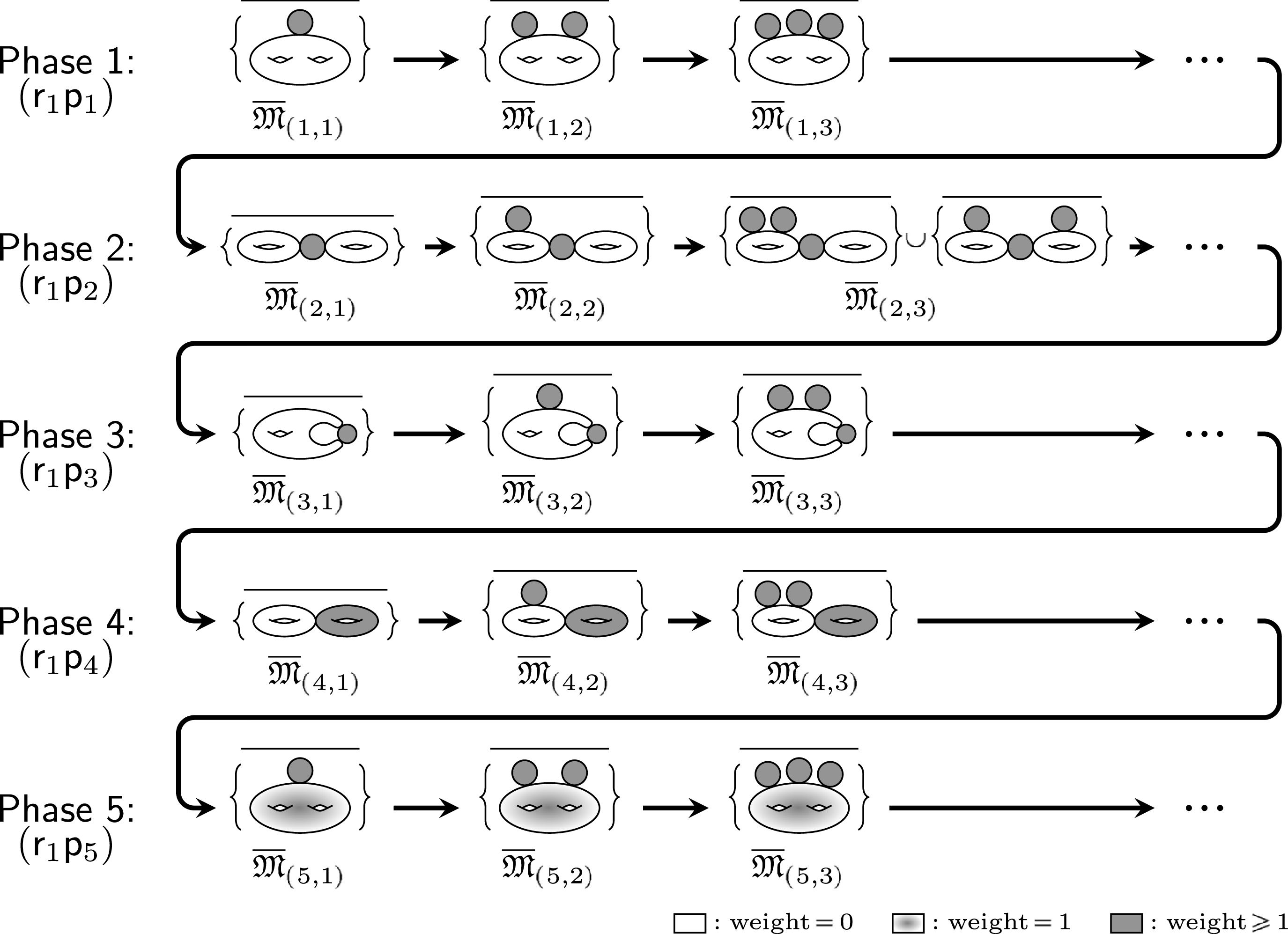
 r1
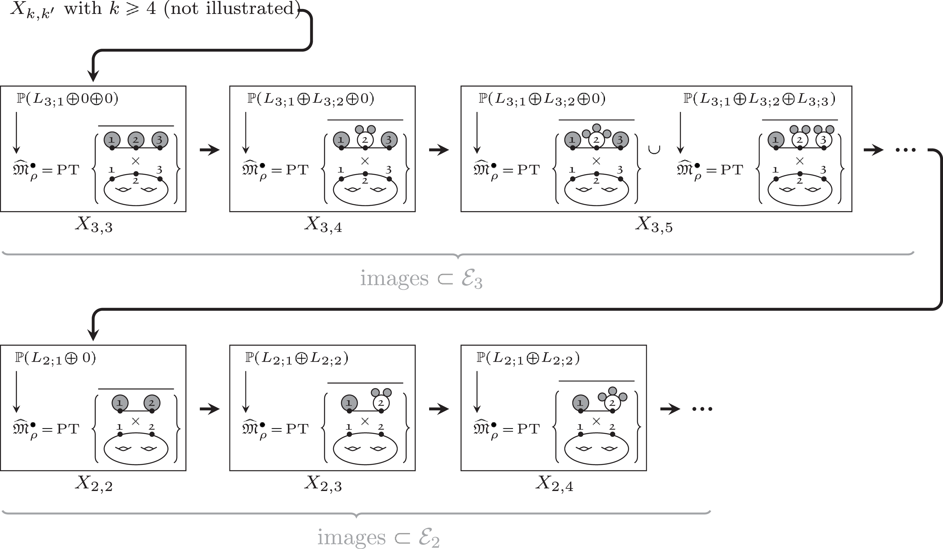
 (r2)
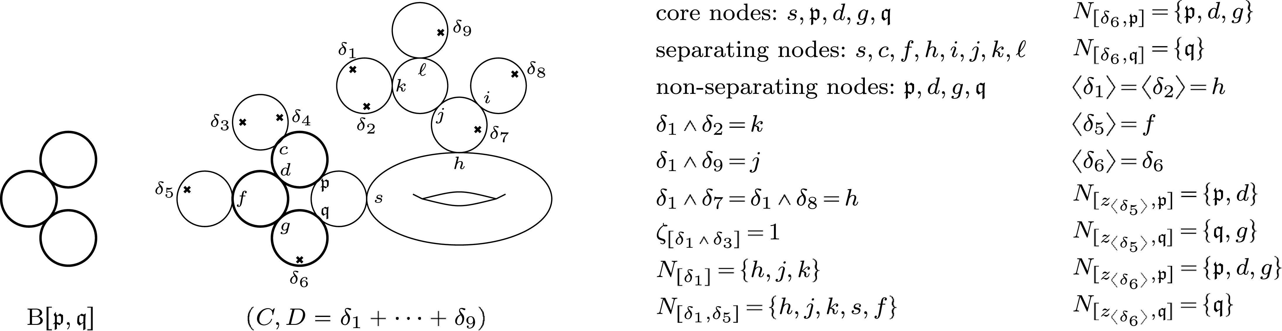
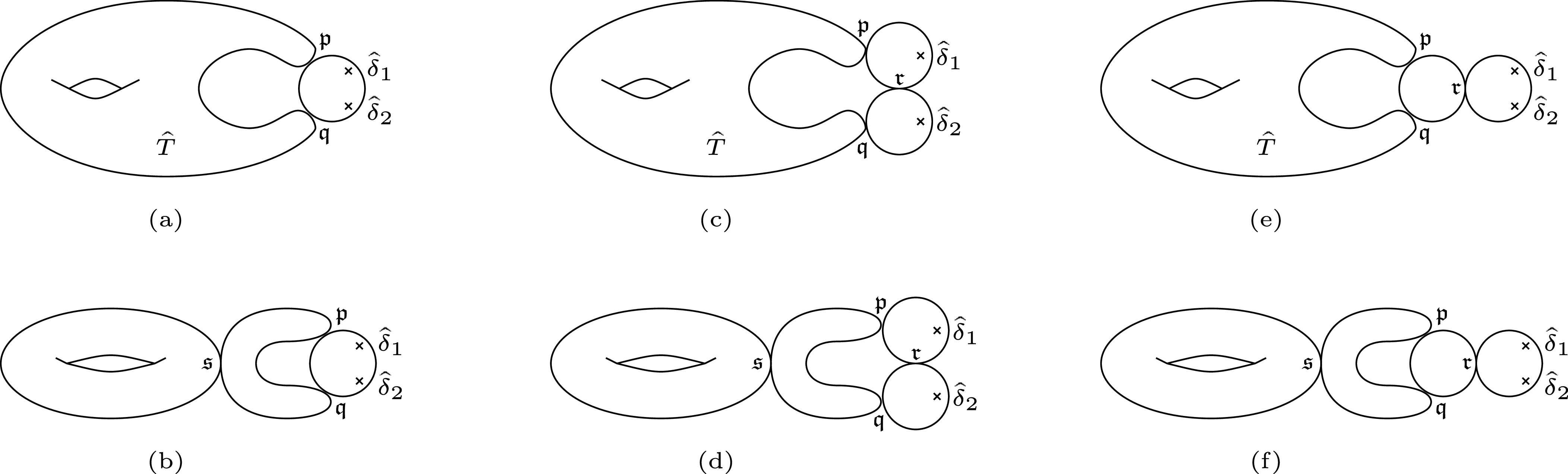
 (C^,δ^1,δ^2)∈K¯
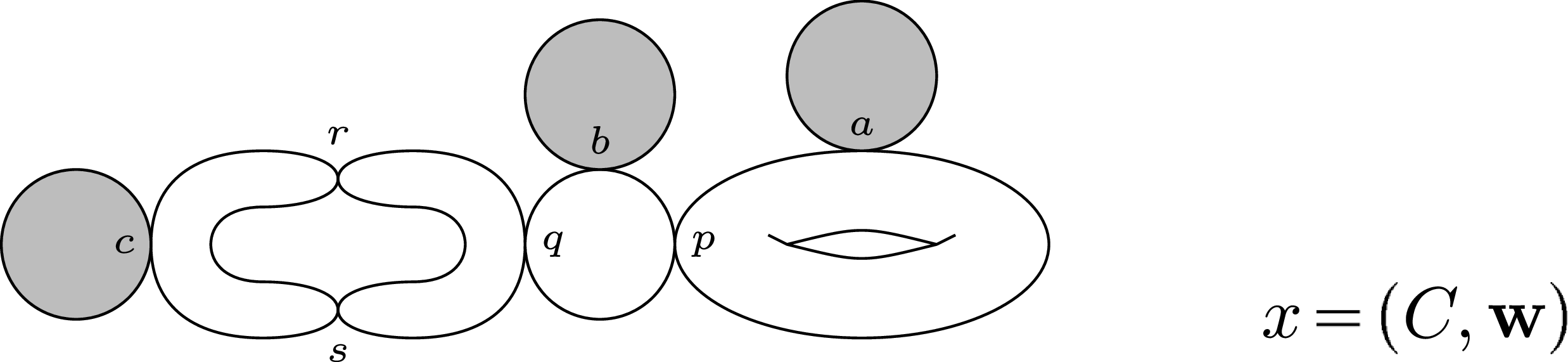
 M¯(i,k)
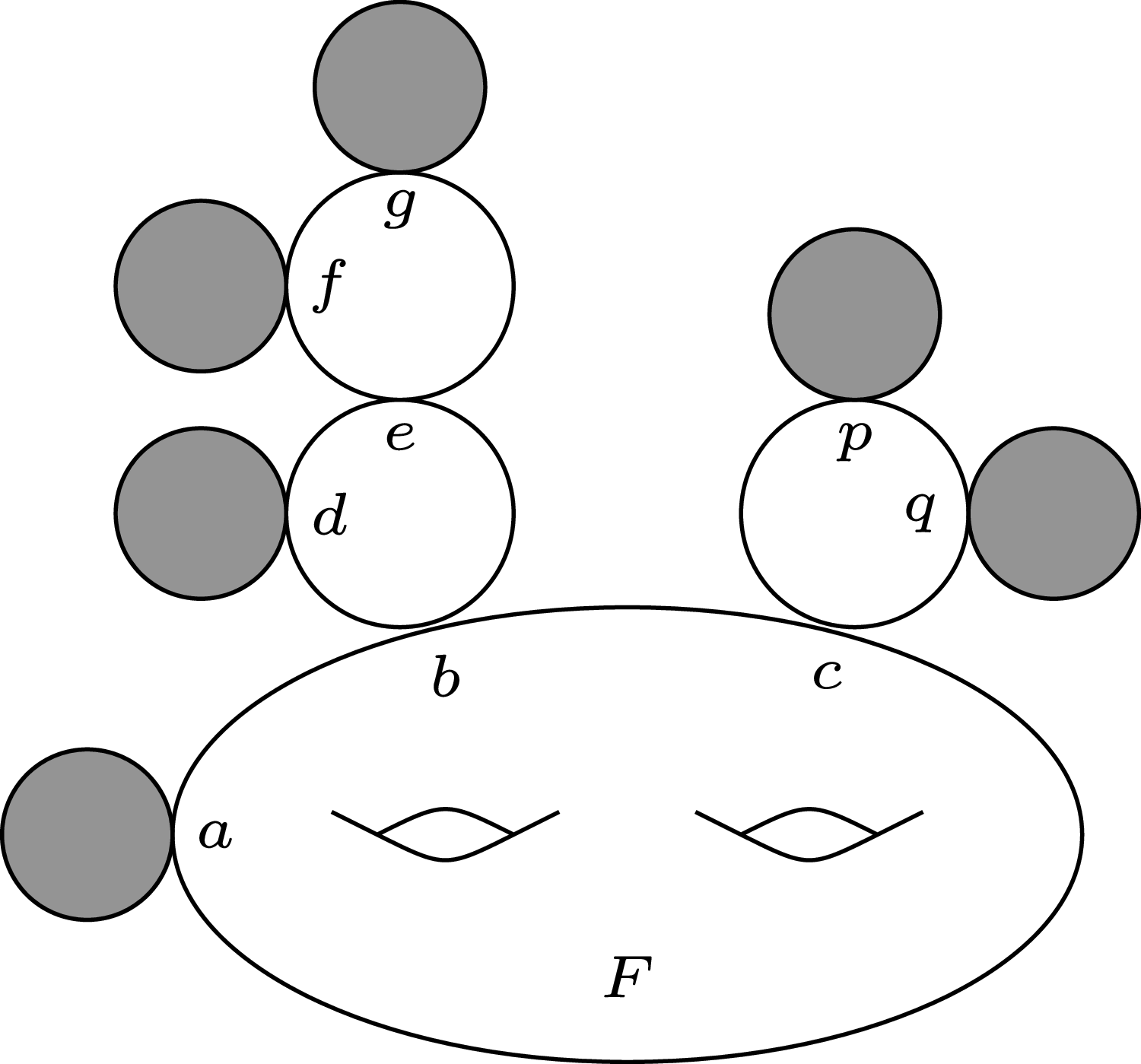
 C
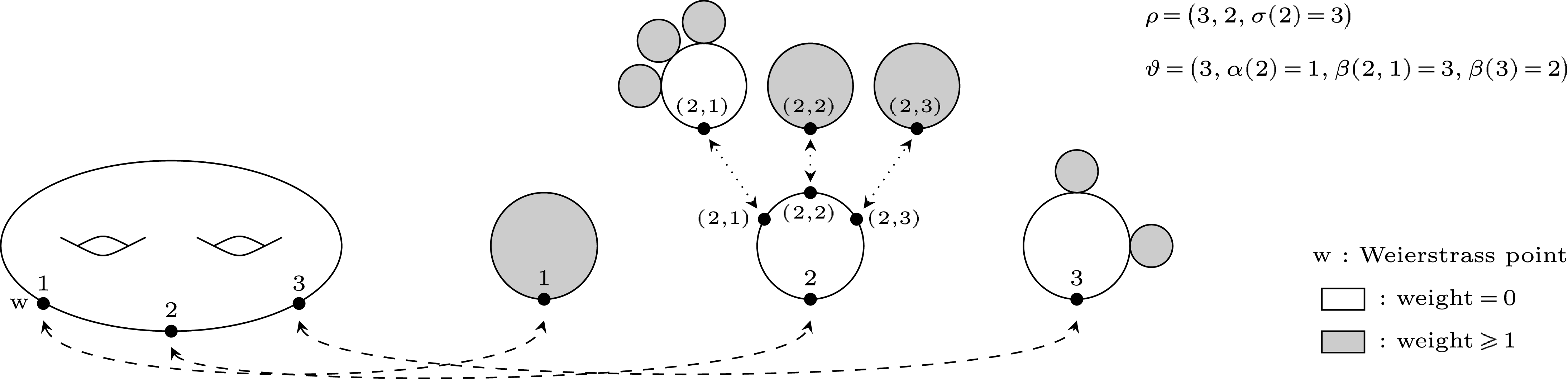
 W^ρ,ϑ
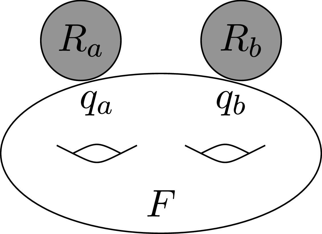
 C
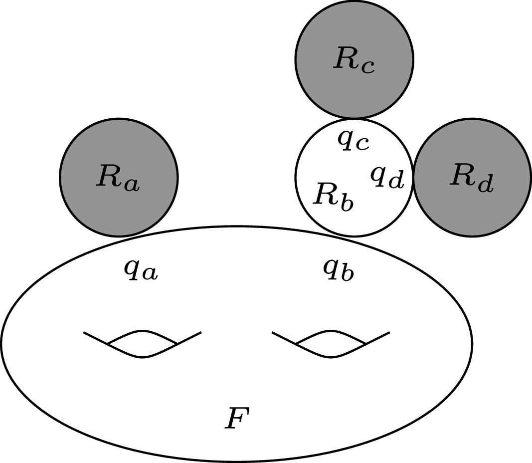
 C
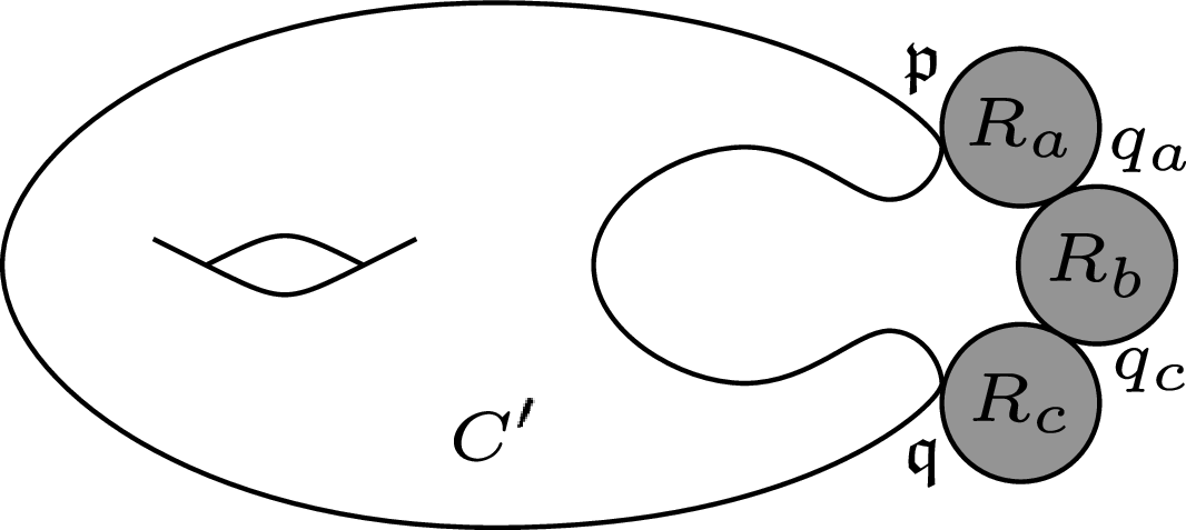
 C
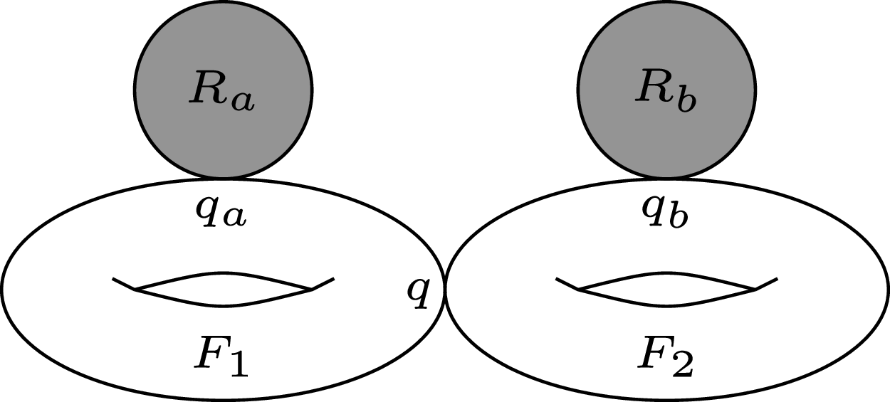
 C
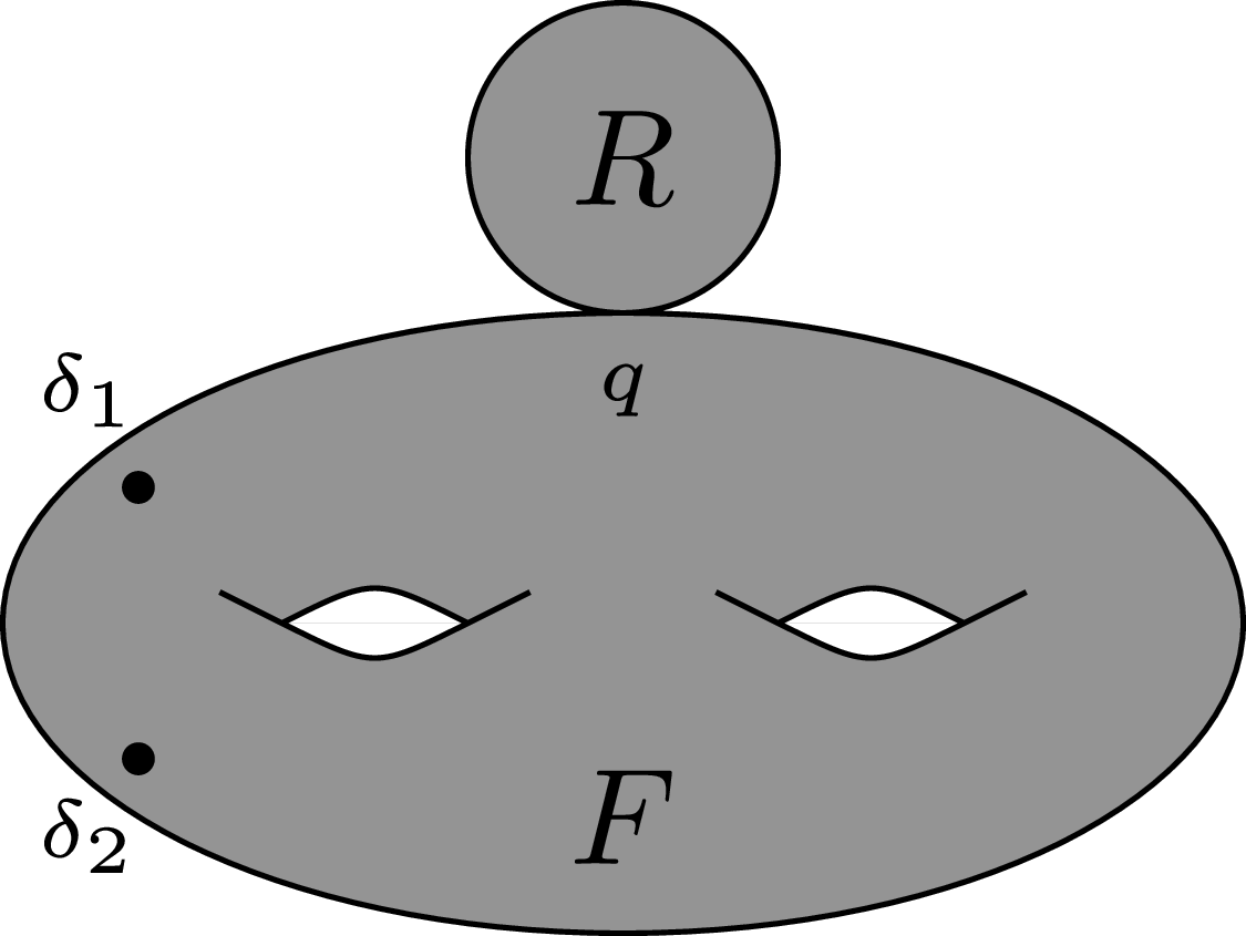
 (C,D)

 τ
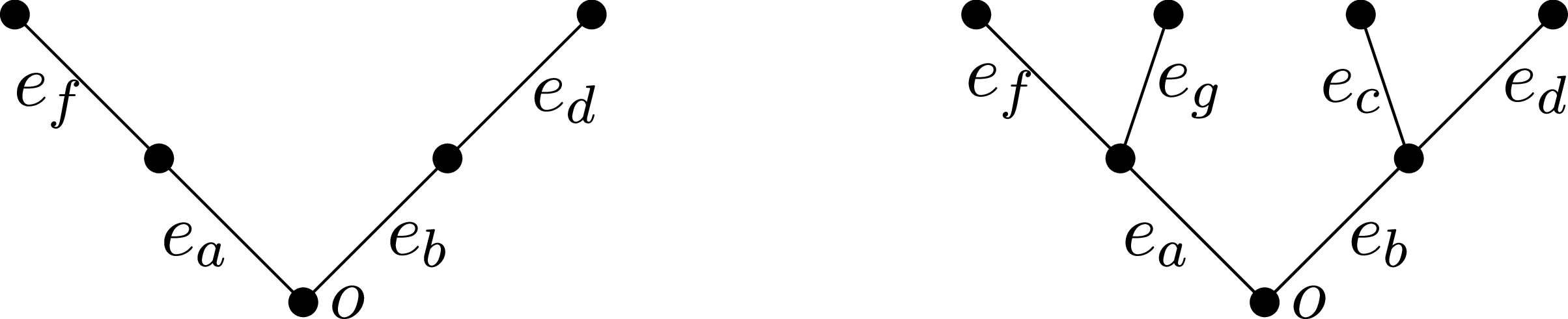
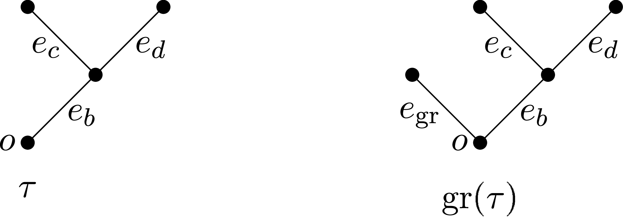
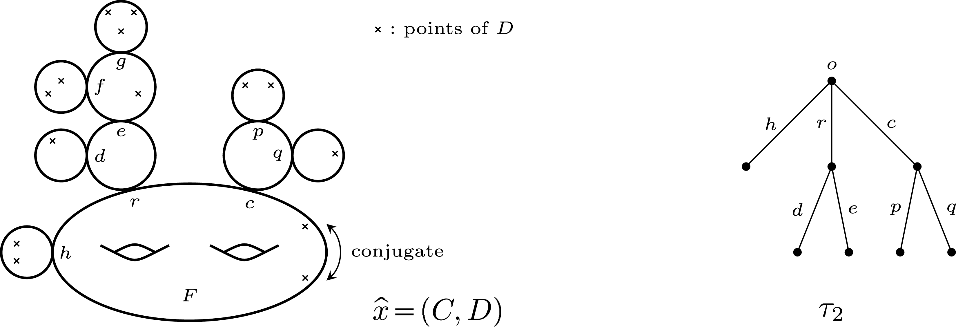
 τ2
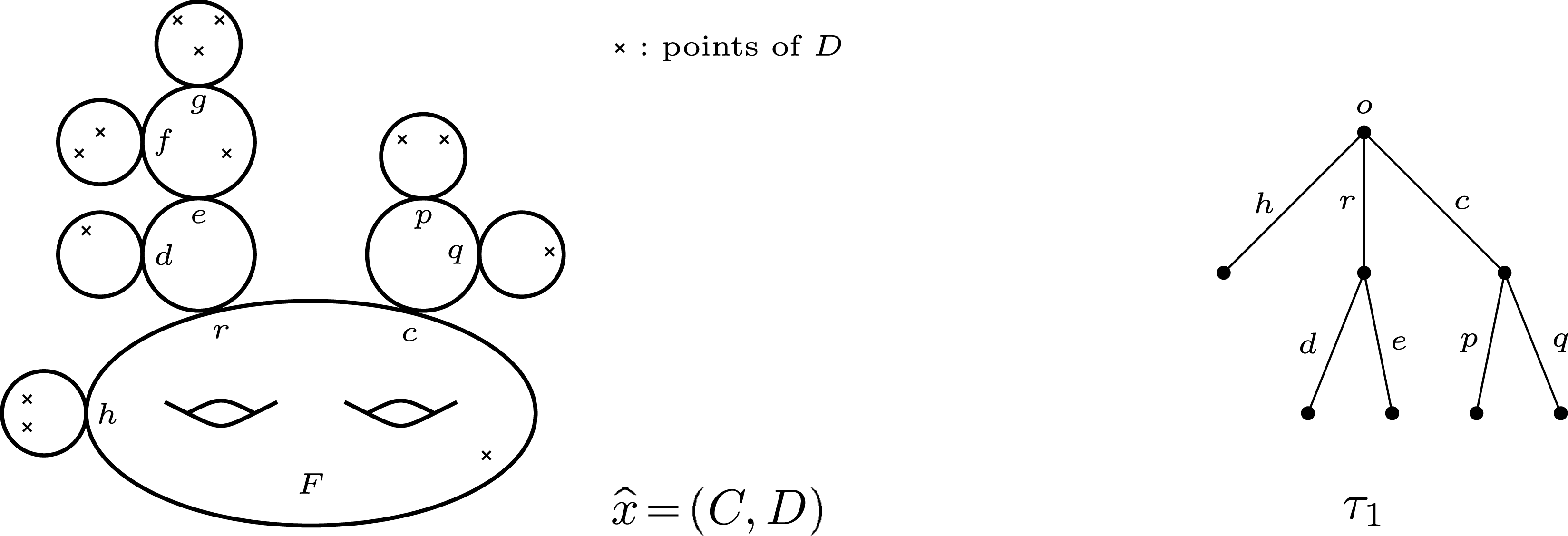
 τ1
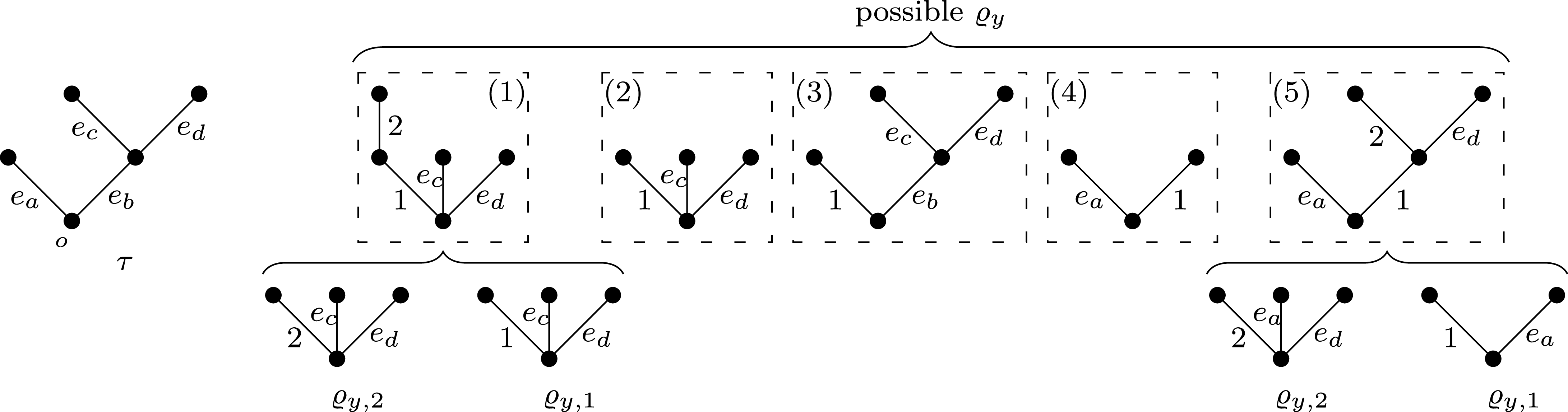

 τ†

 τ‡

 τ∧
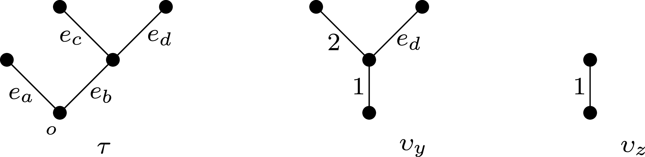


 Open access

