2. NPSML FOR STATIC MODELS

Simulation-based methods are clearly most useful in dynamic settings. Nevertheless, it seems simpler to introduce the NPSML method and its asymptotic properties within a static model. Therefore, consider a model with reduced form

where θ, the parameter of interest, belongs to a compact set

, the observed endogenous variable y is a vector of

, the exogenous variable x belongs to

represents the disturbances. We assume that both the function g and the distribution of the disturbances ε are fully known.

Let (x_t,y_t)_t=1,…,T be an independent and identically distributed (i.i.d.) sample. The associated log likelihood then is

denoting l_t(θ) the density of y_t knowing (x_t,θ). We make the following assumption.

Assumption L1. The maximum likelihood estimator

is consistent, asymptotically normal, and asymptotically efficient. The true parameter θ₀ belongs to the interior of Θ. More precisely, we assume that for some positive definite matrix Ω,

uniformly with respect to θ* in a neighborhood of θ₀, and that

For the class of models we are interested in, the likelihood function l_t(θ) cannot be computed in a closed form, so that it is impossible to compute the maximum likelihood estimator

. We propose instead to approximate each term l_t(θ) by a kernel estimator based on some i.i.d. simulated sample (ε_t^s)_s=1,…,S drawn from the distribution

Thus, denoting y_t^s(θ) = g(x_t,θ,ε_t^s), the likelihood l_t(θ) is estimated by

Here, h is a bandwidth such that h → 0 when S → ∞, and K is a kernel. To simplify the presentation, assume that h is a power of S and that S is bounded above and below by powers of T. Under technical conditions that are stated subsequently, l_t^S(θ) converges to l_t(θ) when the number of simulations S goes to infinity. Thus a natural idea consists in defining the NPSML estimator as the global maximizer of

on Θ. It can be obtained using standard maximization algorithms; note that because l_t^S is a combination of kernels and the latter usually are smooth and have a simple form, it is easy to feed analytical derivatives into the maximization routine to reduce the computation time if need be.

Because the logarithm has infinite derivative in zero, small simulation errors on small values of the likelihood will be amplified. Thus it is necessary to trim the smallest values of l_t^S.⁶

where τ_S is a sufficiently regular function⁷

One example is the continuously differentiable function defined by

when x ∈ [h^δ,2h^δ] . Therefore, this function τ_S is piecewise polynomial and ∥τ_S′∥_∞ = O(h^−δ).

Thus we define the NPSML estimator by

We now state a set of assumptions under which it is strongly consistent when T and S go to infinity and the bandwidth h goes to zero.

To make the structure of our assumptions more apparent, we have employed a simple codification: the letter L is used for regularity conditions on the likelihood, T for the tail behavior of the underlying variables, M for the conditions on the reduced-form model g, R for the rates of convergence of the parameters, and K for the kernel.

The first assumption concerns the kernel. We make the following assumption.

Assumption K1. The kernel K is twice continuously differentiable and has compact support.

Let ρ be the order of the kernel, that is, ∫x₁^α₁…x_m^α_mK(x) dx is zero if

and nonzero if [sum ]_j α_j ∈ {0,ρ}. (Classically, ρ = 2 for positive symmetric kernels.)

We need more assumptions on the exact likelihood function. In addition to Assumption L1, we make the following assumption.

Assumption L2. l(y|x,θ) and ∂^ρl(y|x,θ)/∂y^ρ are bounded above on

. There exists some β > 1 such that a.e.

Moreover

Assumption T1. There exists ν such that

Assumption M1. There exist a function φ and some s₀ ≥ 0 such that

with E [φ(ε)] < ∞, and where ν was introduced in Assumption T1.

More specifically, Assumption L2 is necessary to bound uniformly some bias terms in kernel smoothing. It could be weakened.⁸

Our technical assumptions could be weakened by assuming that the exogenous variables x belong to a bounded subset. We think this is too restrictive. Thus, in this paper, the support of the joint law of (x_t,y_t) is a priori unbounded, even if this makes the assumptions uglier and the proofs longer and more involved.

We also need to put some assumptions on the order of the trimming function and the rate of convergence of the bandwidth to zero as the number of simulation draws goes to infinity. Trimming aside, this is the usual assumption in nonparametric density estimation.

Assumption R1. δ < ρ and Sh^m+2δ/ln S goes to infinity as S goes to infinity.

We can finally state our consistency theorem.

THEOREM 2.1. Under Assumptions K1, L1 and L2, T1, M1, and R1,

is strongly consistent: a.e.,

It is easy to check that

is weakly consistent under the same assumptions except the second part of R1 and replacing (2.7) by E [sup_θ|ln l_t(θ)|^β] < ∞.

To apply our estimation method in practice, it is necessary to fix the values of the parameters ρ, δ, K, h, ν, and S. The main difficulty consists in choosing the rates of convergence of the number of simulations S to infinity and of the bandwidth h to zero so that the assumptions of Theorem 2.1 hold. Let us therefore assume that S = C₁T^a and h = C₂ S^−b for some positive constants C₁ and C₂.

We would like to ensure the consistency of the NPSML estimator. We neglect Assumption T1, which is bound to hold if the density of (x,y) is not too thick-tailed.⁹

In particular, take the usual case of a second-order kernel (ρ = 2). Then we can choose δ = 1, for instance, and the asymptotically optimal bandwidth selector for kernel density estimation, for which b = 1/(m + 4), fits the bill. Thus the most natural choice for the rate of convergence of h to zero yields a consistent NPSML estimator. Note that as expected, the speed of convergence of S to infinity then is irrelevant for consistency: we only require that a > 0.

To prove the asymptotic normality and efficiency of the NPSML estimator, we need to strengthen the previous assumptions. To state them, let V₀ denote a neighborhood of θ₀.

Assumption L3. There exist γ > 1 and γ′ > 1 such that

Moreover, ∂^ρ+1l(y|x,θ)/∂θ∂y^ρ is bounded on

.

Assumption T2. For some ν > 0,

tends to zero when S and T tend to infinity, where γ and γ′ (resp. ζ) were introduced in Assumption L3 (resp. M2).

Assumption M2. For some r₀ ≥ 0 and some p₀ > 4,

Moreover, there exist a function ψ and a number s₁ ≥ 0 such that, for every ε > 0,

Finally, for some ζ > 1,

The number of simulations S has to grow sufficiently quickly with T for T2 to be satisfied. Again, if the derivatives of g are bounded, then one can take r₀ = s₁ = 0 in Assumption M2. The assumptions on the rates of convergence also have to be strengthened.

Assumption R2.

To control the frequency of the trimming, we need the following assumption.

Assumption R3.

where γ was introduced in Assumption L3.

Recall that we denote Ω the asymptotic variance-covariance matrix of the exact maximum likelihood estimator. We can finally state our asymptotic efficiency theorem.

THEOREM 2.2. Under Assumptions K1, M1 and M2, L1–L3, R1–R3, and T1 and T2,

is asymptotically normal and asymptotically efficient:

where Ω was defined in Assumption L1.

To simplify the proof, we have used assumptions that are more restrictive than need be. Also, the assumptions used imply that

is strongly consistent, whereas convergence in probability would suffice.

When this theorem applies,

has the same asymptotic variance as

, the exact maximum likelihood estimator of θ₀. Thus

is asymptotically efficient and Ω can be estimated by

Now consider the assumptions required to get asymptotic normality, still assuming S = C₁T^a and h = C₂ S^−b. In addition to R1, R2 and R3 must also hold. R2 translates into

Now choose ρ > δ and some C₀ > 1/2(ρ − δ). Moving on the hyperbola ab = C₀ to the zone of large a and small b will satisfy all assumptions. Thus our conditions define a nondegenerate region of the (a,b) plane. One would hope that this region intersects the line b = 1/(m + 2ρ) that defines the usual asymptotically optimal bandwidth. It can be checked that such is the case if (ρ − δ) is large enough, which may imply using higher order kernels (ρ > 2).

Assumption R3 is more problematic, as it should be checked on a case-by-case basis. Clearly, it holds when h goes to zero fast enough.

To illustrate the technical assumptions, we verify them for the simplest model we could imagine, say,

Here, y_t is univariate, normally distributed with mean x_t′ β and variance σ ∈ [σ₁,σ₂], σ₁ > 0. Because l_t(θ) is Lipschitz-continuous with respect to the parameters, some uniform strong laws of large numbers are available to get L2. Assumption T1 is true for every ν > 0. To get M1 when x_t is unbounded, it is sufficient that hS^ν → 0, which is the case with a sufficiently small ν. Thus, to satisfy R1 and to obtain the consistency of

, set δ = 1, ρ = 2, and b < 1/3. To get the asymptotic normality, note that L3, T2, and M2 are true for every choice of γ, γ′, and ζ. Tedious calculations show that R3 holds if

which is satisfied for ab > γ/2δ(γ − 1). Because R2 implies ab > ½, choose a = 6 and

, for instance. To get more realistic rates for S and h, it is necessary to increase ρ, namely, to consider higher order kernels.

3. EXTENSION TO LIMITED DEPENDENT VARIABLE MODELS

The theory can be extended to the case when the endogenous variables y_t take some discrete values with a strictly positive probability. Because limited dependent variable models come in many guises, we illustrate the basic idea with the example of the censored regression model

where the univariate latent variable z_t is generated by

Let z_t^s(θ) be the simulated values for the latent variable. When we observe y_t > 0, then the likelihood can be approximated as in Section 2 by

When y_t = 0, then we need to approximate not a density but the probability that z_t is negative. We could just use the empirical proportion of negative z_t^s(θ), but that would not be smooth in the parameters. It seems far better to stick to our kernel-based approach and to define

where

is the integrated kernel

Clearly, this estimator of the required probability converges faster than the estimator of the density. Therefore, the full simulated log likelihood is

The approach sketched here can obviously be generalized to other LDV models. Consider, for instance, the multinomial discrete choice model for which McFadden (1989) develops the simulated method of moments. For individual t, the utility of alternative j = 1,…,p is

and alternative j is chosen if and only if z_jt ≥ z_kt for all k ≠ j. We simulate z_jt^s(θ) in the obvious way, and we use the integrated kernel again to approximate the probability that individual t chooses alternative j by

More generally, the same methodology applies when y_t is vector-valued and when its distribution conditional on x_t has some atoms. By integrating the simulated likelihood for the latent model on some convenient subsets, we get the simulated likelihood for the observations (y_t,x_t). Theorems 2.1 and 2.2 continue to apply.

are exactly the same as previously. The details are left to the reader. To deal with estimators of probability masses, we provide only the technical lemmas in Appendix A (Lemmas A.5 and A.6). Note that, when the endogenous variable y takes discrete values only like in the multinomial discrete choice model, m can be taken equal to zero. Thus, the conditions for consistency and asymptotic normality of the NPSML estimator are weaker in this case (Assumptions R1 and R2 especially).

4. NPSML FOR THE DYNAMIC CASE

As mentioned before, the analysis in Section 2 applies directly to models in which x_t contains lagged observable endogenous variables (provided that ε_t is not serially correlated). However, there is a class of models for which dynamic simulations are called for. This includes

• models with both lagged observable endogenous variables and serially correlated disturbances
• models with lagged latent variables.

An example of the latter is the Tobit model with an autoregressive latent variable process (from now on the “autoregressive Tobit model”), which can be written (in its simplest form)

where y_t represents the observed endogenous variable, z_t is the latent variable, and ε_t is i.i.d. normal with zero mean and unit variance.

In these models, the likelihood function for observation t is a t-dimensional integral, which can very rarely be computed in closed form. For very simple instances of these models, it is possible to apply clever tricks to use simulated maximum likelihood or the method of simulated scores, but there exists as yet no fully general method. As we shall now see, it is possible to extend the NPSML method to these models to obtain a consistent and asymptotically normal estimator, with some loss in asymptotic efficiency.

We generate dynamic simulations of the autoregressive Tobit model as follows. Denote θ = (a,b,σ). For each t, draw ε_t^s in the assumed distribution of ε_t for s = 1…,S. Also draw z₀^s(θ) from the stationary distribution of the latent variable process implied by θ. Then compute recursively

Given the simulated paths of the observable endogenous variables y_t^s(θ), we could proceed exactly as for the static model. This would approximate the marginals

of the likelihood function. If the parameters are identifiable from the marginals, then given technical conditions, the maximum likelihood estimator based on the marginals is consistent. This follows from applying Jensen's inequality to the Kullback criterion. To see this, denote E₀ the expectation with respect to the true marginal l(y_t;θ₀). Then

so that E₀ log l(y_t;θ) is maximal for θ = θ₀. However, this estimator uses only a small part of the information contained in the sample under study. In fact, it is easy to see that in the autoregressive Tobit model, θ is not identifiable from the marginals, as the stationary distribution of z_t is

which only identifies two combinations of the three parameters.

On the other hand, it is easy to see that in the autoregressive Tobit model, θ is identified from the second-order marginal l(y_t,y_t−1,θ). This suggests an approach due to Azzalini (1983) and also applied by Laroque and Salanié (1993): we generalize our earlier procedure by choosing some integer k > 0 and approximating the likelihood of (y_t,…,y_t−k) (in a continuous model here) by

where K is a well-chosen (k + 1)-dimensional kernel and h is a bandwidth.

then is obtained as usual by maximizing

Note that we could also approximate the conditional form of the (k + 1)-order likelihood

Another interesting variant that will be used in our Monte-Carlo simulation circumvents the curse of dimensionality by maximizing

We cannot claim asymptotic efficiency with any of these dynamic methods, because we are only approximating (k + 1)-order marginals of the likelihood function. Nevertheless, the NPSML estimator will be close to asymptotically efficient if these marginals contain about as much information as the full likelihood function. Of course, the curse of dimensionality will severely limit the possible values of k, to, say, 1 or 2. Therefore it is an empirical question whether the efficiency loss is large or not in any particular model.

This procedure clearly extends to more general models whose reduced form can be written as

where the vector of endogenous variables z_t may contain

• observable endogenous variables y_t
• latent endogenous variables y_t*
• disturbances ε_t.

Now u_t represents the innovations in the disturbances and is still assumed to be drawn from a known distribution

. For instance, we might have

where both ρ₁ and σ are parameters to be estimated. Dynamic simulations then are obtained, given an initializing scheme for z₀^s(θ), by computing for s = 1,…,S and t = 1…,T

where the u_t^s are drawn from

. This generates the y_t^s(θ) that are the basis for the dynamic NPSML method.

Theorems 2.1 and 2.2 can be adapted to the dynamic framework; one may also prove that when the number of lags k tends to infinity at the right speed when T goes to infinity, then the NPSML estimator is asymptotically efficient. Indeed, the key tool of the proofs is Lemma A.1, which can be extended to the dynamic case. There are two main caveats here. First, θ₀ must be identifiable from the marginal likelihood function l(y_t,…,y_t−k;θ). There is clearly no general argument as to what value of k will achieve identification; this must be checked for each specific model.¹³

where J is the derivative of the score and I is the outer product of the scores, corrected for serial correlation. Moreover, the notation becomes messier and the assumptions must be strengthened. There are in fact so many technical differences between the static and the dynamic cases that another paper seems to be necessary to state and prove the asymptotic properties of the dynamic NPSML estimators. Therefore we do not include the proof here. It seems more interesting to examine how well these methods perform in practice. To this end, we now turn to a Monte-Carlo simulation study of the finite-sample properties of the dynamic NPSML estimator as applied to the autoregressive Tobit model.

5. A MONTE-CARLO SIMULATION EXPERIMENT

Latent variable models in which the latent variable is serially correlated are a natural area for applying NPSML because they usually give rise to analytically untractable likelihood functions. We study here the properties of the NPSML estimators of the autoregressive Tobit model discussed previously, both on time series and on panel data.

There are some choices to be made when applying the NPSML method. We used the normal kernel to nonparametrically estimate the density, and we did not prewhiten the data. We chose the bandwidth h by applying Silverman's rule for the bandwidth that minimizes the mean integrated square error for a normal density. We trimmed the 5% smallest values of the likelihood. These choices could presumably be improved upon in a real-life application, but they seem to be a reasonable starting point.

The autoregressive Tobit model is defined on time series by

where the true values of the parameters are a = 0, b = 0.5, and σ = 1 and ε_t is i.i.d. normal with zero mean and unit variance. This model can describe, for instance, the evolution of prices on a market with a regulated price floor (as with some farm products in developed economies).

We ran a Monte-Carlo experiment for k = 1. We chose a sample size of T = 150 and generated 500 samples of artificial data. The initial parameter values were drawn from the uniform distribution on [−0.2, 0.2] for a, from the uniform distribution on [0.25, 0.75] for b, and from the uniform distribution on [0.5, 1.5] for σ. For each parameter vector reached during maximization, the initial value of the latent variable z₀ was drawn from the stationary distribution implied by these parameter values.

Table 1 summarizes the results for S = 50 and S = 500. The estimation takes on average 2 seconds for S = 50 and 7 seconds for S = 500 on a Pentium 1.4 GHz PC using Gauss.¹⁴

Simulation on time series

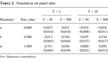
Of course, most applications of the Tobit model use panel data. NPSML can equally well be applied to such data, although this time the asymptotic theory applies for large I (the number of individuals) and fixed T. To test the properties of NPSML on panel data, we use a sample of sizes I = 1,000 and T = 2 or T = 10. Again, we use 500 artificial samples, except for T = 10 and S = 500, for which we only generated 250 samples.¹⁵

Simulation on panel data

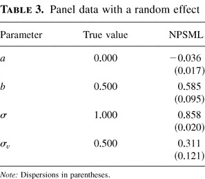
To conclude this illustrative Monte-Carlo study, we add a random individual effect in the autoregressive Tobit model. Thus our model now is

where the parameters are as before except that v_i is drawn from a centered normal distribution with true standard error σ_v = 0.5. This is a much more challenging model, as we have to disentangle the serial correlation induced by b ≠ 0 and that induced by the v_i, while only observing y_it. In fact, it is easy to see that the model is only identifiable for T ≥ 3. A consequence is that we now need to choose k ≥ 2 in our NPSML estimation. For experimental purposes, we took T = 10 and we maximized the simulated analog of

using k = 5 and S = 500 simulations.¹⁶

Panel data with a random effect

6. CONCLUDING REMARKS

Although the NPSML method has very appealing statistical properties in static models, its real test lies in its ability to give good estimates in finite samples for dynamic models. The method works reasonably well for the autoregressive Tobit model, which is a tough test for any estimation method. The most remarkable aspect of NPSML is its generality: the method is essentially the same for all econometric models. It is very easy to implement: it takes less than 40 program lines to define the function to be maximized, and only about 10 lines need to be changed when estimating a different model. Of course, such a general estimation method cannot compete with methods that exploit the particular features of a specific model, but it seems to offer a good product of performance and ease of use. Consider, for instance, the stochastic volatility model often used on financial data:

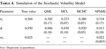
where y_t represents the observed returns and y_t* the latent volatility and (ε_1t,ε_2t) are jointly normal i.i.d. with zero mean and unit variance. Following case 5 of Jacquier, Polson, and Rossi (1994), we study the model with the crucial parameter φ set at 0.95. Table 4 gives the results of running NPSML and three alternative estimation methods,¹⁷

Simulation of the Stochastic Volatility Model

on a 500-observation sample with 500 simulations, and 500 Monte Carlo runs.¹⁸