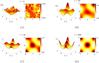
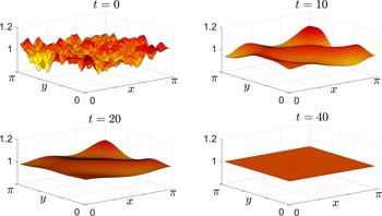
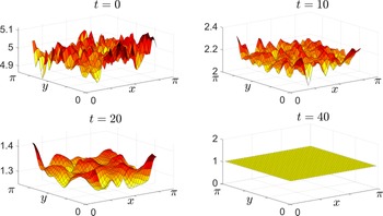
1. Introduction and main results
In this paper, we study the global existence of strong solutions (and also some aspects of the large time behaviour) of the following reaction–diffusion system including chemotaxis terms:
 \begin{equation} \left\{ \begin{aligned} & \partial_t m = \Delta m + m(1-m^{a-1}) - \chi \nabla\cdot(f(m)\nabla c), & & (x,t)\in Q_T,\\ & \partial_t c = \varepsilon_0\Delta c + \delta d - c + \beta m, & & (x,t)\in Q_T,\\ & \partial_t d = g(m)(1-d), & & (x,t)\in Q_T,\\ & \nabla m\cdot \nu =\nabla c\cdot \nu = 0, & & (x,t)\in \partial\Omega\times(0,T),\\ & m(x,0) = m_0(x), c(x,0) = c_0(x), d(x,0) = d_0(x), & & x\in\Omega , \end{aligned} \right. \end{equation}
where  $\Omega \subset \mathbb {R}^{n}$ is a bounded domain with smooth boundary
 $\partial \Omega$,
 $Q_T := \Omega \times (0,T)$,
 $\nu$ is the outward normal vector to
 $\partial \Omega$ at a point of
 $\partial \Omega$, the parameters satisfy
 $a>1$, and
 $\chi , \varepsilon _0, \delta , \beta > 0$, and the initial data is nonnegative, bounded and sufficiently smooth. The nonlinearities
 $f$ and
 $g$ satisfy some conditions which will be specified later.
The system (1.1) with
 \begin{equation} a = 2, \quad f(m) = \frac{m}{1+m} \quad \text{ and } \quad g(m) = \frac{rm^{2}}{1+m}, \; r>0, \end{equation}
was recently proposed [Reference Lombardo, Barresi, Bilotta, Gargano, Pantano and Sammartino12] for the dynamics of multiple sclerosis. There,  $m := m(x,t) \ge 0$ is the density of inflammatory immune cells (macrophages),
 $c := c(x,t) \ge 0$ is the density of a chemoattractant (cytokine), and
 $d := d(x,t) \ge 0$ is the density of destroyed oligodendrocytes. This model generalizes that of [Reference Calvez and Khonsari3] and [Reference Khonsari and Calvez10] to describe a rare and aggressive form of multiple sclerosis, namely Baló's sclerosis. It has been shown that by varying the parameter values within realistic ranges taken from the experimental literature, this model is able to reproduce different pathological scenarios typical of the disease ([Reference Bilotta, Gargano, Giunta, Lombardo, Pantano and Sammartino1], [Reference Bilotta, Gargano, Giunta, Lombardo, Pantano and Sammartino2]). The analysis of (1.1)–(1.2) has been carried out in two recent works: in [Reference Desvillettes and Giunta5], the global existence of very weak and classical solutions to (1.1)–(1.2) was shown in dimension one; global classical solutions in higher dimensions are shown in [Reference Hu, Fu and Ai9] under the smallness assumption of the chemoattractant coefficient
 $\chi$ (when
 $n>3$). This latter work also shows that the solution is bounded uniformly in time, and the positive equilibrium is globally asymptotically stable if
 $\chi$ is small enough.
In the present work, we study (1.1) with a general logistic growth of order  $a>1$, and the nonlinearities
 $f$ and
 $g$ are assumed to satisfy
(F)
 $f\in C^{2}([0,\infty ))$ with $f(0) = 0$, and there exist constants $\gamma , b, \ell \geq 0$ such that
(1.3)\begin{equation} |f(y)| \leq \gamma \, y^{b} \quad \text{ and } \quad |f'(y)|\leq \gamma\, y^{\ell} \quad \text{ for all } \quad y\geq 0 , \end{equation}
(G)
$g\in C^{1}([0,\infty ))$ and $g(y) > 0$ for all $y > 0$.


It's easy to check that the special case (1.2) fulfills the assumptions (F) for  $f$ with
 $b = \ell =0$, and the assumption (G) for
 $g$.
The first main result of this paper concerns the existence and uniqueness of (uniformly w.r.t.  $t$) bounded strong solutions to system (1.1), when the parameter
 $b$ appearing in assumption (1.3) is not too large.
Theorem 1.1 Let  $\Omega$ be a smooth (
 $C^{2+\alpha }$ for some
 $\alpha >0$) bounded connected open subset of
 $\mathbb {R}^{n}$ (for
 $n \in \mathbb {N} - \{0\}$), and suppose
 $a>1$,
 $\chi , \varepsilon _0, \delta , \beta > 0$,
 $\gamma , b, l \ge 0$, and the functions
 $f$ and
 $g$ satisfy (F) and (G). We further assume
 \begin{equation} \max\left\{{b-1,\frac b2}\right\} < \frac{a}{n+2}, \end{equation}
and consider nonnegative initial data  $(m_0, c_0, d_0)\in W^{(2-2/\tilde {p}),\tilde p}(\Omega )\times W^{(2-2/\tilde {p}),\tilde p} (\Omega )\times L^{\infty }(\Omega )$, for some
 $\tilde {p}>\max \{n+2,a\}$. Then, system (1.1) has a unique nonnegative (for each component) strong solution which is bounded uniformly in time. More precisely,
 $\partial _t m$,
 $\partial _t c$,
 $\partial _t d$,
 $\Delta m$,
 $\Delta c$,
 $\nabla \cdot (f(m)\nabla c)$ belong to
 $L^{\tilde p}(\Omega \times (0,T))$ for all
 $T>0$, and there exists
 $C>0$ (depending on
 $\Omega$,
 $n$,
 $a$,
 $b$,
 $\varepsilon _0$,
 $\beta$,
 $\delta$,
 $m_0$,
 $c_0$,
 $d_0$), and
 $\tilde C>0$ (depending on
 $\Omega$,
 $n$,
 $a$,
 $b$,
 $\varepsilon _0$,
 $\beta$,
 $\delta$,
 $d_0$), such that
 \begin{equation} \sup_{t\geq 0}\left({\|m({\cdot} , t)\|_{L^{\infty}(\Omega)}+\|c({\cdot} , t)\|_{W^{1,\infty}(\Omega)}+\|d({\cdot} , t)\|_{L^{\infty}(\Omega)}}\right) \leq C, \end{equation}
and
 \begin{equation} \limsup_{t\to \infty}\left({\|m({\cdot} , t)\|_{L^{\infty}(\Omega)}+\|c({\cdot} , t)\|_{W^{1,\infty}(\Omega)}+\|d({\cdot} , t)\|_{L^{\infty}(\Omega)}}\right) \leq \tilde C. \end{equation}
Finally, if the initial data are smooth, i.e.  $m_0, c_0, d_0 \in C^{2}(\overline {\Omega })$ and satisfy compatibility conditions
 $\nabla m_0 \cdot \nu = \nabla c_0 \cdot \nu = 0$ on
 $\partial \Omega$, then the solution is classical. That is
 \[ \partial_tm, \partial_tc, \partial_td, \Delta m, \Delta c, \nabla\cdot(f(m)\nabla c) \in C^{0}(\overline{\Omega}\times [0,T]) \]
for all  $T>0$.
Remark 1.2 The difference between  $C$ and
 $\tilde {C}$ in (1.5) and (1.6) is that
 $\tilde {C}$ does not depend on
 $m_0$ and
 $c_0$. This means that in large time, the bound of solutions depends only on the size of
 $d_0$ but not
 $m_0$ and
 $c_0$.
For the special case (1.2), since  $b = 0$ and
 $a = 2$, condition (1.4) is satisfied in all dimensions. Therefore, theorem 1.1 in particular shows that the system (1.1)–(1.2) has global unique strong solutions (for suitable initial data) in all dimensions. We also emphasize that theorem 1.1 improves the global existence in [Reference Hu, Fu and Ai9] by removing the requirement that
 $\chi$ is small in all cases.
Let us briefly describe the ideas underlying the proof of theorem 1.1. Using the comparison principle, it's easy to show that  $d$ is bounded uniformly in time and space. It follows straightforwardly from the logistic term that
 $m$ is bounded in
 $L^{a}(\Omega \times (0,T))$. Using these bounds and the properties of the heat equation satisfied by
 $c$, thanks to its linearity, we obtain some
 $L^{q}(\Omega \times (0,T))$ bound for
 $\nabla c$. In order to use this estimate in the equation satisfied by
 $m$, we exploit the so-called duality method, which proved its significant usefulness in the study of reaction-diffusion systems (cf. [Reference Cañizo, Desvillettes and Fellner4, Reference Morgan and Quoc Tang13, Reference Pierre14]), or cross diffusion systems ([Reference Desvillettes, Lepoutre, Moussa and Trescases6, Reference Desvillettes and Trescases7]). Under condition (1.4), the duality method yields an
 $L^{p}(\Omega \times (0,T))$ estimate for
 $m$ for all
 $1\leq p < \infty$. This information and a bootstrap argument allow us to conclude that
 $c$ is bounded in
 $L^{\infty }(0,T;W^{1,\infty }(\Omega ))$ and that
 $m$ is bounded in
 $L^{\infty }(\Omega \times (0,T))$, hence the global existence of bounded solutions to (1.1). To show the uniform-in-time bound (1.5), we use a smooth truncation function in time to study (1.1) on each cylinder
 $\Omega \times (\tau ,\tau +1)$,
 $\tau \in \mathbb {N}$. We repeat the previous arguments to obtain that
 $m$ and
 $c$ are bounded in
 $\Omega \times (\tau ,\tau +1)$ uniformly in
 $\tau \in \mathbb {N}$, which consequently implies the desired bounds (1.5) and (1.6). It's worth noting that this uniform-in-time bound plays an important role in the nonlinear stability, which is discussed in the following paragraphs.
Our second main result of this paper is the nonlinear exponential stability of a positive (for all components) homogeneous equilibrium. A homogeneous equilibrium  $(m^{*},c^{*},d^{*})$ to (1.1) solves
 $m^{*} = (m^{*})^{a}$,
 $\delta d^{*} + \beta m^{*} = c^{*}$ and
 $g(m^{*})(1-d^{*}) = 0$. It's straightforward that
 \[ (\bar m, \bar c, \bar d) = (1, \beta +\delta,1) \]
is the unique positive (for all components) homogeneous equilibrium. Besides this, we also have other equilibria, namely:
 \[ (m^{*},c^{*},d^{*}) = \begin{cases} (0,\delta,1) & \text{ if } g(0)\ne 0,\\ (0,\delta\zeta,\zeta) \text{ with } \zeta \geq 0 \text{ arbitrary } & \text{ if } g(0) = 0. \end{cases} \]
Theorem 1.3 Exponential nonlinear stability of  $(\bar {m}, \bar {c}, \bar {d})$
Let the assumptions of theorem 1.1 hold and assume additionally that  $f(1)>0$. If
 \begin{equation} \chi < \chi_{\mathrm{subcrit}} := \frac{4\sqrt{\varepsilon_0(a-1)}}{\beta f(1)}, \end{equation}
then the constant steady state  $(\bar {m}, \bar {c}, \bar {d})$ is exponentially asymptotically stable. More precisely, there exists
 $\varepsilon >0$ such that if
 $(m_0,c_0,d_0)\in W^{(2-2/\tilde {p}),\tilde {p}}(\Omega )\times W^{(2-2/\tilde {p}),\tilde {p}}(\Omega )\times L^{\infty }(\Omega )$ for
 $\tilde {p}>\max \{n+2,a\}$, and
 \[ \|m_0 - \bar{m}\|_{L^{2}(\Omega)} + \|c_0 - \bar{c}\|_{L^{2}(\Omega)} + \|d_0 - \bar{d}\|_{L^{2}(\Omega)} \leq \varepsilon, \]
then for all  $p\in [1, \infty [$ and
 $\delta \in ]0, 1]$, there exist
 $C, \varrho > 0$ depending on
 $p$ and
 $\delta$ such that
 \[ \left\|{m(t) - \bar{m}}\right\|_{L^{p}(\Omega)} + \left\|{c(t) - \bar{c}}\right\|_{W^{1 - \delta,p}(\Omega)} + \left\|{d(t) - \bar{d}}\right\|_{L^{p}(\Omega)} \leq C \,e^{-\varrho t} \quad \text{ for all } t\geq 0. \]
Remark 1.4 We expect that the nonlinear stability in theorem 1.3 can be shown under the optimal condition  $\chi < \chi _c$, where
 $\chi _c$ is defined in (3.2) using the eigenvalues of the Laplacian with Neumann boundary condition (see § 3 for more details). We remark that the threshold (1.7) becomes optimal when
 $\varepsilon _0^{-1} = a-1$, which makes
 $\chi _{\mathrm {subcrit}} = \chi _{c0}$ (see (3.3)).
To prove theorem 1.3, we first rewrite system (1.1) with a new variable  $(\tilde {m}, \tilde {c}, \tilde {d}) = (m - \bar m, c - \bar c, d - \bar d)$. Next, we show that under condition (1.7), the linear part, after a suitable scaling, has a spectral gap. This spectral gap and the uniform-in-time bound proved in theorem 1.1 allow us to show that the nonlinear part is dominated by the linear one, and consequently obtain the nonlinear stability of
 $(\bar m, \bar c, \bar d)$.
The organization of the paper is as follows: In § 2, we prove theorem 1.1 by first showing global existence, then uniqueness, and finally the uniform-in-time bound. In § 3.1, we prove the nonlinear stability in theorem 1.3. Then, in § 3.2 we perform numerical simulations on a 2D spatial domain to show Turing patterns which appear for sufficiently large chemoattractant coefficient  $\chi$. Finally, § 3.3 concludes the paper with a presentation of open problems relevant for the model under study.
Notation. Throughout this paper, we use the following notations
• The space
$L^{p}(\Omega )$, $1\leq p\leq \infty$, is equipped with the norm
and\[ \|v\|_{L^{p}(\Omega)} = \left({\int_{\Omega}|v(x)|^{p}\,\textrm{d}x}\right)^{\frac 1p} \quad \text{ when } \quad p<\infty, \]\[ \|v\|_{L^{\infty}(\Omega)} = \underset{x\in\Omega}{\mathrm{ess\, sup}}|v(x)|. \]• When
$1\leq p\leq \infty$ and $r>0$ is an integer, we define the space
and when\[ W^{r,p}(\Omega) := \left\{{v\in L^{p}(\Omega): \partial_x^{s}v \in L^{p}(Q_{\tau,T}) \text{ for } s\in \mathbb{N} \text{ with } s \leq r}\right\}, \]$r$ is not an integer, we use the definition in [Reference Ladyženskaija, Alekseevich Solonnikov and Uralceva11, chapter 2, section 2].• For any
$0\leq \tau < T$, $Q_{\tau ,T} := \Omega \times (\tau ,T)$. When $\tau = 0$, we write $Q_T$ instead of $Q_{0,T}$.• The space-time space
$L^{p}(Q_{\tau ,T}) = L^{p}((\tau ,T);L^{p}(\Omega ))$, $1\leq p\leq \infty$, is equipped with the norm
and\[ \|v\|_{L^{p}(Q_{\tau,T})} = \left({\int_{\tau}^{T}\int_{\Omega}|v(x,t)|^{p}\,\textrm{d}x\,\textrm{d}t}\right)^{\frac 1p} \quad \text{ when } \quad p<\infty, \]\[ \|v\|_{L^{\infty}(Q_{\tau,T})} = \underset{(x,t)\in Q_{\tau,T}}{\mathrm{ess\, sup}}|v(x,t)|. \]• We denote the space-time space
equipped with the norm\begin{align*} W^{2,1}_{p}(Q_{\tau,T}) &:= \{v\in L^{p}(Q_{\tau,T}): \partial_t^{r}\partial_x^{s}v \in L^{p}(Q_{\tau,T}) \text{ for}\\ &\quad \times r,s\in \mathbb{N} \text{ with } 2r + s \leq 2\}, \end{align*}\[ \|v\|_{W^{2,1}_{p}(Q_{\tau,T})} := \sum_{2r+s\leq 2}\left\|{\partial_t^{r}\partial_x^{s} v}\right\|_{L^{p}(Q_{\tau,T})}. \]


2. Proof of theorem 1.1
2.1 Global existence of bounded solutions
In this subsection, we show the existence of solutions to system (1.1) which are bounded on  $Q_T$ for all
 $T>0$.
The following lemma is useful in our analysis.
Lemma 2.1 ([Reference Ladyženskaija, Alekseevich Solonnikov and Uralceva11, lemma 3.3] and [Reference Simon15, theorem 3])
Assume  $1< p<\infty$. There exists a constant
 $C>0$, only depending on
 $T-\tau ,\Omega ,p,n$, such that for all
 $v\in W_p^{2,1}(Q_{\tau ,T})$,
(a)
where\[ \left\|{v}\right\|_{L^{q}(Q_{\tau,T})} \leq C\, \left\|{v}\right\|_{W^{2,1}_p(Q_{\tau,T})} \]\[ q = \begin{cases} \dfrac{(n+2)p}{n+2-2p} & \text{ if } p<(n+2)/2,\\ <{+}\infty \text{ arbitrary } & \text{ if } p = (n+2)/2,\\ +\infty & \text{ if } p > (n+2)/2. \end{cases} \](b)
where\[ \left\|{\nabla v}\right\|_{L^{q}(Q_{\tau,T})} \leq C\, \left\|{v}\right\|_{W^{2,1}_p(Q_{\tau,T})} \]\[ q = \begin{cases} \dfrac{(n+2)p}{n+2-p} & \text{ if } p< n+2,\\ <{+}\infty \text{ arbitrary } & \text{ if } p = n+2,\\ +\infty & \text{ if } p > n+2. \end{cases} \]


Furthermore, when  $p>n+2$, the space
 $W_p^{2,1}(Q_{\tau ,T})$ is compactly embedded in
 $C^{1,0}(\overline \Omega \times [0,T])$.
Next, we prove the
Proposition 2.2 Under the assumptions of theorem 1.1, and picking  $T>0$, system (1.1) has a nonnegative (for each component) strong solution which is bounded on
 $Q_T$. More precisely, there exists
 $C_T>0$ (depending on
 $\Omega$,
 $T$,
 $n$,
 $a$,
 $b$,
 $\varepsilon _0$,
 $\beta$,
 $\delta$,
 $\|m_0\|_{L^{\infty }(\Omega )}$,
 $\|c_0\|_{W^{ 1,\infty }(\Omega )}$,
 $\|d_0\|_{L^{\infty }(\Omega )}$), such that
 \begin{equation} \|m\|_{L^{\infty}(Q_T)}+\|c\|_{L^{\infty}((0,T); W^{1,\infty}(\Omega))}+\|d\|_{L^{\infty}(Q_T)} \leq C_T. \end{equation}
Proof of proposition 2.2 For a given  $r>0$, define
 $h_r \in C^{\infty }(\mathbb {R}_+,[0,1])$ such that
 $h_r(y) = 1$ for
 $0\leq y\leq r$, and
 $h_r(y) = 0$ for
 $y\geq 2r$. We also use the standard convention
 $m_+ := \max \{0; m\}$. Consider the system
 \begin{equation} \left\{ \begin{aligned} & \partial_t m =\Delta m + m_+(1-m_+^{a-1}) - \chi\nabla\cdot(f_r(m_+)\nabla c), & & (x,t)\in Q_T,\\ & \partial_t c = \varepsilon_0 \Delta c + \delta d - c + \beta m_+, & & (x,t)\in Q_T,\\ & \partial_t d = g(m_+)(1-d), & & (x,t)\in Q_T,\\ & \nabla m\cdot \nu = \nabla c\cdot \nu = 0, & & (x,t)\in \partial\Omega\times(0,T),\\ & m(x,0) = m_0(x), \,\, c(x,0) = c_0(x), \,\, d(x,0) = d_0(x), & & x\in\Omega, \end{aligned} \right. \end{equation}
where the function  $f_r$ is defined as
 \[ f_r(y) := h_r(f(y)). \]
We will prove, thanks to Leray-Schauder's theorem (cf. [Reference Gilbarg and Trudinger8, theorem 10.3]), that (2.2) has a nonnegative (for each component) solution which is bounded in sup-norm independent of  $r>0$, and consequently prove the existence of a solution to the original system (1.1) on
 $Q_T$. To this end, we define
 \[ \mathfrak{Y}:= C^{1,0}(\overline\Omega\times [0,T] ) \quad \text{ and } \mathfrak{X} := \mathfrak{Y}\times \mathfrak{Y}, \]
where  $C^{1,0}$ is the space of continuous functions such that their gradient (with respect to space) is also continuous, associated with the natural norm (making it a Banach space)
 \[ \|u\|_{\mathfrak{Y}} = \sup_{t\in[0,T]}\|u(t)\|_{L^{\infty}(\Omega)} + \sup_{t\in [0,T]}\|\nabla u(t)\|_{L^{\infty}(\Omega)}, \]
and
 \[ \mathcal{F}_r: \mathfrak{X} \times [0,1] \to \mathfrak{X} \quad \text{ via } \quad \mathcal{F}_r(m,c, \lambda):= (\lambda\,\mathfrak{M}, \lambda\, \mathfrak{C}), \]
where  $(\mathfrak {M},\mathfrak {C})$ is given (in a unique way) by solving first an ODE (for
 $d$), and then successively (for
 $\mathfrak {C}$ and
 $\mathfrak {M}$, in that order) two Neumann problems for the heat equation with a source. More precisely,
 $(\mathfrak {M},\mathfrak {C})$ is the (unique) solution on
 $Q_T$ of the system
 \begin{equation} \left\{ \begin{aligned} & \partial_t \mathfrak{M} = \Delta \mathfrak{M} + m_+\left({1-m_+^{a-1}}\right) - \chi \nabla\cdot(f_r(m_+)\nabla \mathfrak{C}), & & (x,t)\in Q_T,\\ & \partial_t \mathfrak{C} = \varepsilon_0 \Delta \mathfrak{C} + \delta d - \mathfrak{C} + \beta m_+, & & (x,t)\in Q_T,\\ & \partial_t d = g(m_+)(1-d), & & (x,t)\in Q_T,\\ & \nabla\mathfrak{M} \cdot \nu = \nabla \mathfrak{C} \cdot \nu = 0, & & (x,t)\in \partial\Omega\times(0,T),\\ & \mathfrak{M}(x,0) = m_0(x), \mathfrak{C}(x,0) = c_0(x), d(x,0) = d_0(x), & & x\in\Omega. \end{aligned} \right. \end{equation}
Note first that  $\mathcal {F}_r(m,c, 0) = 0$. Then, regardless of
 $m$, we always have that
 \begin{equation} 0 \leq d(x,t) \leq \mu := \max\left\{{1, \|d_0\|_{L^{\infty}(\Omega)}}\right\}. \end{equation}
Also for any  $1< p\le \tilde p$, there exists
 $C_p>0$ depending on
 $\|m\|_{\mathfrak {Y}}$ and
 $r$ (and
 $\Omega , T, m_0, c_0, \mu$) such that, thanks to maximal regularity results,
 \begin{equation} \|\mathfrak{C}\|_{W^{2,1}_{p}(Q_T)} \leq C_p, \end{equation}
and
 \begin{equation} \|\mathfrak{M}\|_{W^{2,1}_{p}(Q_T)} \leq C_p. \end{equation}
Thanks to the embedding in lemma 2.1,
 \begin{equation} W^{2,1}_p(Q_T) \hookrightarrow \mathfrak{Y} \text{ compactly when } p >n+2. \end{equation}
So, we see that since  $\tilde p>n+2$, the map
 $\mathcal {F}_r$ sends bounded sets in
 $\mathfrak {X}$ into compact sets of
 $\mathfrak {X}$. We now show that for any
 $\lambda \in [0,1]$,
 $\mathcal {F}_r(\cdot ,\cdot ,\lambda )$ is continuous from
 $\mathfrak {X}$ to
 $\mathfrak {X}$. Let
 $(m_1, c_1), (m_2,c_2)\in \mathfrak {X}$ and
 $(\lambda \mathfrak {M}_1, \lambda \mathfrak {C}_1)= \mathcal {F}_r(m_1,c_1,\lambda )$,
 $(\lambda \mathfrak {M}_2,\lambda \mathfrak {C}_2) = \mathcal {F}_r(m_2,c_2,\lambda )$. We have
 \begin{align} \begin{cases} \partial_t(\mathfrak{M}_1 - \mathfrak{M}_2) &= \Delta(\mathfrak{M}_1 - \mathfrak{M}_2) + \left[{m_{1+}(1-m_{1+}^{a-1}) - m_{2+}(1-m_{2+}^{a-1}) }\right]\\ &\quad + \chi\nabla\cdot\left[{f_r(m_{1+})\nabla \mathfrak{C}_1 - f_r(m_{2+})\nabla \mathfrak{C}_2}\right],\\ \partial_t(\mathfrak{C}_1 - \mathfrak{C}_2) &= \varepsilon_0\Delta (\mathfrak{C}_1 - \mathfrak{C}_2) + \delta(d_1 - d_2) - (\mathfrak{C}_1 - \mathfrak{C}_2) + \beta(m_{1+} - m_{2+}),\\ (d_1 - d_2)_t &= g(m_{1+})(1-d_1) - g(m_{2+})(1-d_2). \end{cases} \end{align}
By rewriting  $g(m_{1+})(1-d_1) - g(m_{2+})(1-d_2)$
 $= g(m_{1+})(d_2 - d_1) + (g(m_{1+}) - g(m_{2+}))\, (1-d_2)$, and using
 $g\in C^{1}([0,\infty ))$, we obtain
 \[ d_1(x,t) - d_2(x,t) = \int_0^{t}e^{-\int_{s}^{t}g(m_{1+}(r))dr}g'(\theta(x, s))(m_{1+}(s)-m_{2+}(s))(1\,{-}\,d_2(s))\,\textrm{d}s,\]
where  $\theta (x,s)$ is between
 $m_{1+}(x,s)$ and
 $m_{2+}(x,s)$. Therefore, there exists
 $C_T>0$ (which can depend on the norm
 $\|m_{1}\|_{\mathfrak {Y}}$) such that
 \[ \|d_1 - d_2\|_{L^{\infty}(Q_T)} \leq C_{T}\|m_{1+} - m_{2+}\|_{L^{\infty}(Q_T)} \leq C_T\|m_{1}-m_{2}\|_{\mathfrak{Y}}. \]
By maximal regularity results and (2.7)
 \begin{align} \|\mathfrak{C}_1 - \mathfrak{C}_2\|_{\mathfrak{Y}} &\leq C_T\|\mathfrak{C}_1 - \mathfrak{C}_2\|_{W^{2,1}_p(Q_T)}\notag\\ & \leq C_T\left({\|d_1-d_2\|_{L^{p}(Q_T)} + \|m_{1+} - m_{2+}\|_{L^{p}(Q_T}}\right)\notag\\ & \leq C_T\|m_{1} - m_{2}\|_{\mathfrak{Y}}. \end{align}
For the equation satisfied by  $\mathfrak {M}_1 - \mathfrak {M}_2$, we write
 \[ \left|{m_{1+}(1-m_{1+}^{a-1}) - m_{2+}(1-m_{2+}^{a-1})}\right| \le \left|{m_{1} - m_{2}}\right| + \left|{m_{1} - m_{2}}\right|\, \max(m_{1+}^{a-1}, m_{2+}^{a-1}), \]
and
 \begin{align*} & \left|{\nabla\cdot\left[{f_r(m_{1+})\nabla \mathfrak{C}_1 - f_r(m_{2+})\nabla \mathfrak{C}_2}\right]}\right|\\ & \quad\le \left|{f_r(m_{1+})}\right|\left|{\Delta(\mathfrak{C}_1 - \mathfrak{C}_2)}\right| + \left|{f_r(m_{1+})- f_r(m_{2+})}\right|\left|{\Delta \mathfrak{C}_2}\right|\\ &\qquad + \left|{f_r'(m_{1+})}\right|\left|{\nabla m_{1+}}\right|\left|{\nabla(\mathfrak{C}_1-\mathfrak{C}_2)}\right|\\ & \qquad + \left|{f_r'(m_{1+})}\right|\left|{\nabla(m_{1+}-m_{2+})}\right|\left|{\nabla \mathfrak{C}_2}\right| + \left|{f_r'(m_{1+}) - f_r'(m_{2+})}\right|\left|{\nabla m_{2+}}\right|\left|{\nabla \mathfrak{C}_2}\right| . \end{align*}
Using the fact that  $f\in C^{2}([0,\infty ))$, estimate (2.9), and maximal regularity results we get
 \begin{equation} \|\mathfrak{M}_1 - \mathfrak{M}_2\|_{\mathfrak{Y}} \leq C_T\|\mathfrak{M}_1 - \mathfrak{M}_2\|_{W^{2,1}_{\tilde p}(Q_T)} \leq C_T\|m_{1}-m_{2}\|_{\mathfrak{Y}}. \end{equation}
It follows from (2.9) and (2.10) that  $\mathcal {F}_r(\cdot ,\cdot ,\lambda )$ is continuous from
 $\mathfrak {X}$ to
 $\mathfrak {X}$ for any
 $\lambda \in [0,1]$.
We now check the last assumption in Leray-Schauder's theorem. We consider therefore
 \begin{equation} \mathbf{Z}:= \left\{{(m,c)\in \mathfrak{X} \,:\, (m,c) = \mathcal{F}_r(m,c, \lambda) \; \text{ where } \; 0<\lambda \leq 1 }\right\}, \end{equation}
and will show that  $\mathbf {Z}$ is bounded in
 $\mathfrak {X}$.
Note that if  $(m,c)\in \mathbf {Z}$, then
 $(m,c) = (\lambda \mathfrak {M}, \lambda \mathfrak {C})$, where
 $(\mathfrak {M},\mathfrak {C})$ solves (2.3). Therefore, by multiplying the equations in (2.3) by
 $\lambda$, we obtain (for
 $(m,c) \in \mathbf {Z}$)
 \begin{align} \left\{ \begin{aligned} & \partial_t m = \Delta m + \lambda\left[{m_+(1-m_+^{a-1}) - \chi\nabla\cdot(f_r(m_+)\nabla \mathfrak{C})}\right], & & (x,t)\in Q_T,\\ & \partial_t c = \varepsilon_0\Delta c - c + \lambda(\delta d + \beta m_+), & & (x,t)\in Q_T,\\ & \partial_t d = g(m_+)(1-d), & & (x,t)\in Q_T,\\ & \nabla m\cdot \nu =\nabla c\cdot \nu = 0, & & (x,t)\in \partial\Omega\times(0,T),\\ & m(x,0) = \lambda m_0(x), c(x,0) = \lambda c_0(x), d(x,0) = d_0(x), & & x\in\Omega. \end{aligned} \right. \end{align}
Since  $d\geq 0$,
 $m_+\geq 0$, and
 $c_0 \geq 0$, we obtain immediately (for
 $(m,c) \in \mathbf {Z}$) that
 $c\geq 0$. We now show that
 $m$ is also nonnegative. Indeed, denote by
 $m_- = \max \{0,-m\}$, and multiply the equation satisfied by
 $m$ in (2.12) by
 $(m_-)^{2}$. Then, an integration by parts and the fact
 $m_-m_+ = 0$ give for all
 $t \in [0,T]$,
 \[ -\frac 13\int_{\Omega}m_-^{3}(x,t)\,\textrm{d}x - 2\int_0^{t}\int_{\Omega}m_-|\nabla m_-|^{2}\,\textrm{d}x\,\textrm{d}s \geq 0. \]
Therefore,  $m_- = 0$ and thus
 $m\geq 0$. It follows from the nonnegativity of
 $m$,
 $c$ and
 $d$ (and system (2.12)) that
 $(m,c,d)$ solves the system
 \begin{equation} \left\{ \begin{aligned} & \partial_t m = \Delta m + \lambda m(1-m^{a-1}) - \chi\nabla\cdot(f_r(m)\nabla c), & & (x,t)\in Q_T,\\ & \partial_t c = \varepsilon_0\Delta c - c + \lambda(\delta d + \beta m), & & (x,t)\in Q_T,\\ & \partial_t d = g(m)(1-d), & & (x,t)\in Q_T,\\ & \nabla m\cdot \nu =\nabla c\cdot \nu = 0, & & (x,t)\in \partial\Omega\times(0,T),\\ & m(x,0) = \lambda m_0(x), c(x,0) = \lambda c_0(x), d(x,0) = d_0(x), & & x\in\Omega. \end{aligned} \right. \end{equation}
In order to show that  $\mathbf {Z}$ is bounded, we propose a series of lemmas. We start with the
Lemma 2.3 Under the assumptions of theorem 1.1, and supposing that  $\lambda \in ]0,1]$, we consider
 $(m,c,d)$ a strong, nonnegative (for each component) solution to (2.13). Then there exists
 $K_1>0$ (depending on
 $T$,
 $a, \beta , \delta$ and
 $\|m_0\|_{L^{1}(\Omega )}$,
 $\|c_0\|_{L^{1}(\Omega )}$,
 $\|d_0\|_{L^{\infty }(\Omega )}$, but not depending on
 $\lambda$) such that
 \begin{equation} \sup_{t\in[0,T]}\left({\|m({\cdot}, t)\|_{L^{1}(\Omega)} + \|c({\cdot}, t)\|_{L^{1}(\Omega)}}\right) \leq K_1, \end{equation}
and if  $0\leq \tau < T$ then
 \[ \|m\|_{L^{a}(Q_{\tau,T})} \leq \left[{K_1(T-\tau+1)}\right]^{1/a}. \]
Proof. Note that
 \begin{equation} \frac{\textrm{d}}{\,\textrm{d}t}\int_{\Omega} (m+c)\,\textrm{d}x = \int_{\Omega}\left[{\lambda(\delta d + (\beta+1)m - m^{a}) - c}\right]\,\textrm{d}x. \end{equation}
Since  $a>1$, there exists
 $k_a>0$ such that
 \[ (\beta+1)m - m^{a} \leq k_a - m. \]
Applying this and the fact that  $0\leq d \leq \mu$ to (2.15), we obtain some
 $K_1>0$ such that (2.14) holds. In addition, integrating the equation satisfied by
 $m$ in (2.13) gives
 \[ \int_{\Omega}m(x,T)\,\textrm{d}x = \int_\tau^{T}\int_{\Omega}\lambda m(1-m^{a-1})\,\textrm{d}x\,\textrm{d}t + \int_{\Omega}m(x,\tau)\,\textrm{d}x. \]
Consequently,
 \begin{equation} \|m\|_{L^{a}(Q_{\tau,T})}^{a} \leq K_1(T-\tau+1). \end{equation}
We now turn to the
Lemma 2.4 Under the assumptions of theorem 1.1, and supposing that  $\lambda \in ]0,1]$, we consider
 $(m,c,d)$ a strong, nonnegative (for each component) solution to (2.13). Then there exists
 $K_2>0$ (depending on
 $\Omega$,
 $T$,
 $n$,
 $a$,
 $\varepsilon _0, \beta , \delta$ and
 $\|c_0\|_{W^{(2-2/a),a}(\Omega )}$,
 $\|d_0\|_{L^{\infty }(\Omega )}$, but not depending on
 $\lambda$) such that
 \begin{equation} \|c\|_{W^{2,1}_{a}(Q_T)} + \|\nabla c\|_{L^{q_1}(Q_T)} \leq K_2\,K_1\,(T+1), \end{equation}
where
 \begin{equation} q_1 = \left\{ \begin{aligned} & \frac{(n+2)a}{n+2-a} & & \text{ if } a < n+2,\\ & <{+}\infty \text{ arbitrary} & & \text{ if } a = n+2, \\ & ={+}\infty & & \text{ if } a > n+2 \end{aligned}\right. \end{equation}

We finally prove the
Lemma 2.5 Under the assumptions of theorem 1.1, and supposing that  $\lambda \in ]0,1]$, we consider
 $(m,c,d)$ a strong, nonnegative (for each component) solution to (2.13). Then for any
 $1 \le p<\infty$, there exists
 $F_p^{*}>0$ (depending on
 $\Omega$,
 $T$,
 $n$,
 $p$,
 $a$,
 $b$,
 $\varepsilon _0$,
 $\beta$,
 $\delta$,
 $\|m_0\|_{W^{(2-2/\tilde {p}),\tilde p}(\Omega )}$,
 $\|c_0\|_{W^{(2-2/\tilde {p}),\tilde p}(\Omega )}$,
 $\|d_0\|_{L^{\infty }(\Omega )}$, but not depending on
 $\lambda$) such that
 \begin{equation} \|m\|_{L^{p}(Q_T)} \leq F_p^{*}. \end{equation}
Proof. Note that from (1.4), it follows that there exists  $s\in (0,1)$ (depending on
 $a$,
 $b$,
 $n$ only, and with
 $s$ close to
 $1$ if the inequality in (1.4) is close to being an equality) satisfying
 \begin{equation} b-s < \frac{a}{n+2}, \quad \text{ and } \quad b-s<\frac{2a}{n+2} - 1. \end{equation}
It follows that
 \begin{equation} b < s - 1 + \frac{2a}{n+2} \end{equation}
and
 \begin{equation} (n+2)(b-s)< a. \end{equation}
Note also that
 \[ 1 < \frac{2}{n+2} - \frac{b-s}{a}. \]
Since it is sufficient to prove (2.19) for  $p$ large enough, we pick any
 $p'$ such that
 \begin{equation} 1 < p' < \min\left\{{\frac{n+2}{2}, \frac{2}{n+2} - \frac{b-s}{a}}\right\}. \end{equation}
Let  $\theta \in L^{p'}(Q_T)$ with
 $\theta \geq 0$ and
 $\|\theta \|_{L^{p'}(Q_T)} \leq 1$. Let
 $\phi$ be the unique nonnegative solution to the equation
 \begin{equation} \left\{ \begin{aligned} \partial_t \phi + \Delta \phi & ={-}\theta, & & (x,t)\in Q_T,\\ \nabla\phi \cdot \nu & = 0, & & (x,t)\in \partial\Omega\times(0,T),\\ \phi(x,T) & = 0, & & x\in\Omega. \end{aligned} \right. \end{equation}
To avoid any possible confusion, we remark that (2.24) is a forward heat equation for the function  $\psi (x,s)=\phi (x,T-s)$, with respect to the new time variable
 $s=T-t$. From maximal regularity in [Reference Ladyženskaija, Alekseevich Solonnikov and Uralceva11] and lemma 2.1, we know that there exists
 $C_{p'}>0$ (depending on
 $\Omega$,
 $T$,
 $n$ and
 $p$ only) such that
 \begin{equation} \|\partial_t\phi\|_{L^{p'}(Q_T)} + \|\phi\|_{L^{q_2}(Q_T)} + \|\nabla \phi\|_{L^{q_3}(Q_T)} \leq C_{p'} , \end{equation}
where
 \begin{equation} q_2 = \frac{(n+2)p'}{n+2-2p'} \quad \text{ and } \quad q_3 = \frac{(n+2)p'}{n+2-p'}. \end{equation}
Set  $p = {p'}/({p'-1})$. Then, by using the equation satisfied by
 $m$ in (2.13) and integrating by parts, we have
 \begin{align} \int_0^{T}\int_{\Omega}m\theta \,\textrm{d}x\,\textrm{d}t & = \int_0^{T}\int_{\Omega} m (-\partial_t\phi - \Delta \phi)\,\textrm{d}x\,\textrm{d}t\notag\\ & = \lambda\int_{\Omega}m_0\phi(0)\,\textrm{d}x + \int_0^{T}\int_{\Omega}\phi(\partial_t m - \Delta m)\,\textrm{d}x\,\textrm{d}t\notag\\ & \leq \int_{\Omega}m_0\phi(0)\,\textrm{d}x + \lambda\int_0^{T}\int_{\Omega} \phi m \,\textrm{d}x\,\textrm{d}t + \chi\int_0^{T}\int_{\Omega}f_r(m)\nabla \phi \nabla c \,\textrm{d}x\,\textrm{d}t\notag\\ & \leq \int_{\Omega}m_0\phi(0)\,\textrm{d}x + (I) + (II) , \end{align}
where
 \[ (I) = \int_0^{T}\int_{\Omega}\phi m \,\textrm{d}x\,\textrm{d}t \quad \text{ and } \quad (II) = \chi\int_0^{T}\int_{\Omega}|f_r(m)||\nabla \phi||\nabla c|\,\textrm{d}x\,\textrm{d}t. \]
For the first term on the right-hand side of (2.27), we use
 \[ \|\phi(0)\|_{L^{p'}(\Omega)}^{p'} = \int_{\Omega}\left|\int_0^{T}\partial_t\phi \,\textrm{d}t\right|^{p'}\,\textrm{d}x \leq T^{\frac{1}{p-1}}\|\partial_t\phi\|_{L^{p'}(Q_T)}^{p'} \leq T^{\frac{1}{p-1}}C_{p'}^{p'} \]
thanks to (2.25), in order to estimate
 \begin{equation} \int_{\Omega}m_0\phi(0)\,\textrm{d}x \leq \|m_0\|_{L^{p}(\Omega)}\|\phi(0)\|_{L^{p'}(\Omega)} \leq \|m_0\|_{L^{p}(\Omega)}T^{\frac 1p}C_{p'}. \end{equation}
For the treatment of  $(I)$, we consider two cases.
• Case 1.
$a\geq ({n+2})/{2}$. Note that
Therefore, by using Hölder's inequality, we have (for some\[ a \geq \frac{n+2}{2} \Longrightarrow a > \frac{(n+2)p'}{(n+2)(p'-1) + 2p'} \Longrightarrow \frac{a}{a-1} < \frac{(n+2)p'}{n+2-2p'} = q_2. \]$C_T$ depending only on $\Omega$, $T$, $a$, $n$ and $p$)
(2.29)thanks to (2.16) and (2.25).\begin{align} (I) &\leq \|\phi\|_{L^{\frac{a}{a-1}}(Q_T)}\|m\|_{L^{a}(Q_T)} \leq C_T\, \|\phi\|_{L^{q_2}(Q_T)}\|m\|_{L^{a}(Q_T)}\notag\\ & \leq C_T\,C_{p'}\, [K_1\,(T+1)]^{1/a}, \end{align}• Case 2.
$a< ({n+2})/{2}$. Define $\vartheta = 1 - {2a}/({n+2})$ and note that $0<\vartheta <1$. From Hölder's inequality, there exists $R_{T,|\Omega |}>0$ (depending only on $\Omega$, $T$, $a$, $n$ and $p$) such that
(2.30)using\begin{equation} \begin{aligned} (I) & = \int_0^{T}\int_{\Omega} \phi m^{1-\vartheta}m^{\vartheta}\,\textrm{d}x\,\textrm{d}t\\ & \leq R_{T,|\Omega|}\left({\int_0^{T}\int_{\Omega}\phi^{p'}m^{p'(1-\vartheta)}}\right)^{\frac{1}{p'}}\|m\|_{L^{p}(Q_T)}^{\vartheta}\\ & \leq R_{T,|\Omega|} \, \|\phi\|_{L^{\frac{(n+2)p'}{n+2-2p'}}(Q_T)}\left({\int_0^{T}\int_{\Omega}m^{\frac{(n+2)(1-\vartheta)}{2}}\,\textrm{d}x\,\textrm{d}t}\right)^{\frac{2}{n+2}}\|m\|_{L^{p}(Q_T)}^{\vartheta}\\ & = R_{T,|\Omega|} \, \|\phi\|_{L^{q_2}(Q_T)}\|m\|_{L^{a}(Q_T)}^{(1-\vartheta)}\|m\|_{L^{p}(Q_T)}^{\vartheta}, \end{aligned} \end{equation}(2.31)Therefore,\begin{equation} q_2 = \frac{(n+2)p'}{n+2-2p'} \quad \text{ and } \quad \frac{(n+2)(1-\vartheta)}{2} = a. \end{equation}(2.32)\begin{equation} (I) \leq R_{T,\Omega} \, C_{p'}\left[{K_1(T+1)}\right]^{\frac{1-\vartheta}{a}}\|m\|_{L^{p}(Q_T)}^{\vartheta} . \end{equation}


From these two cases, or more precisely, from (2.29) and (2.32), we have
 \begin{equation} (I) \leq C_T^{*}\,\left({1+\|m\|_{L^{p}(Q_T)}^{\vartheta}}\right) \end{equation}
for some  $0<\vartheta <1$ (depending on
 $a,n$), and
 $C_T^{*}$ (depending on
 $\Omega$,
 $T$,
 $n$,
 $p$,
 $a$,
 $\beta$,
 $\delta$,
 $\|m_0\|_{L^{1}(\Omega )}$,
 $\|c_0\|_{L^{1}(\Omega )}$,
 $\|d_0\|_{L^{\infty }(\Omega )}$, but not depending on
 $\lambda$).
In order to estimate  $(II)$, we write
 \begin{equation} \begin{aligned} (II) & = \chi\int_0^{T}\int_{\Omega}|f_r(m)||\nabla \phi||\nabla c|\,\textrm{d}x\,\textrm{d}t\\ & \le \chi \gamma \int_0^{T}\int_{\Omega}|m|^{b}|\nabla \phi||\nabla c|\,\textrm{d}x\,\textrm{d}t\\ & \leq \chi \gamma \left({\int_0^{T}\int_{\Omega}{m^{b-s}|\nabla \phi| |\nabla c|}^{p'}\,\textrm{d}x\,\textrm{d}t}\right)^{\frac{1}{p'}}\|m\|_{L^{p}(Q_T)}^{s}\\ & = \chi \gamma \left({\int_0^{T}\int_{\Omega}m^{p'(b-s)}|\nabla \phi|^{p'} |\nabla c|^{p'}\,\textrm{d}x\,\textrm{d}t}\right)^{\frac{1}{p'}}\|m\|_{L^{p}(Q_T)}^{s}. \end{aligned} \end{equation}
Note that  $1< p'< n+2$ (see (2.23)). We can use Hölder's inequality to estimate further
 \[ \begin{aligned} (II) & \leq \chi\gamma \, \|\nabla \phi\|_{L^{\frac{(n+2)p'}{n+2-p'}}(Q_T)}\left({\int_0^{T}\int_{\Omega}m^{(n+2)(b-s)}|\nabla c|^{n+2}\,\textrm{d}x\,\textrm{d}t}\right)^{\frac{1}{n+2}}\|m\|_{L^{p}(Q_T)}^{s}\\ & \le \chi\gamma \, \|\nabla \phi\|_{L^{q_3}(Q_T)}\|m\|_{L^{a}(Q_T)}^{b-s}\|\nabla c\|_{L^{q_4}(Q_T)}\|m\|_{L^{p}(Q_T)}^{s}, \end{aligned} \]
where
 \begin{equation} q_4 = \frac{(n+2)a}{a-(n+2)(b-s)} \end{equation}
is well defined since  $(n+2)(b-s) < a$ (see (2.20)). Therefore, we can apply (2.25), (2.16) in order to get
 \begin{equation} (II) \leq \chi \gamma \, C_{p'}\, \left[{K_1(T+1)}\right]^{\frac{b-s}{a}}\|\nabla c\|_{L^{q_4}(Q_T)}\|m\|_{L^{p}(Q_T)}^{s}. \end{equation}
Note that from (2.35) we see that when  $a< n+2$,
 \begin{equation} q_4 = \frac{(n+2)a}{a-(n+2)(b-s)}<\frac{(n+2)a}{n+2-a} = q_1, \end{equation}
and that when  $a\geq n+2$,
 $q_4< q_1$ since
 $q_1<+\infty$ can be chosen arbitrarily. Therefore (for some
 $C_T>0$ depending only on
 $\Omega$,
 $T$,
 $a$,
 $b$,
 $n$),
 \[ \|\nabla c\|_{L^{q_4}(Q_T)} \leq C_T\|\nabla c\|_{L^{q_1}(Q_T)} \leq C_T\, K_2\, K_1\,(T+1), \]
thanks to (2.17). It then follows from (2.36) that
 \begin{equation} (II) \leq D_T^{*}\, \|m\|_{L^{p}(Q_T)}^{s}, \end{equation}
where  $D_T^{*}>0$ only depends on
 $\Omega$,
 $T$,
 $n$,
 $p$,
 $a$,
 $b$,
 $\beta$,
 $\delta$,
 $\varepsilon _0$,
 $\chi$,
 $\gamma$,
 $\|m_0\|_{L^{1}(\Omega )}$,
 $\|c_0\|_{W^{\tilde p, (2-2/\tilde {p})}(\Omega )}$,
 $\|d_0\|_{L^{\infty }(\Omega )}$, but does not depend on
 $\lambda$.
From (2.27), (2.28), (2.33) and (2.38), we get (for  $E^{*} := C_{p'} T^{1/p} + C_T^{*} + D_T^{*}$)
 \[ \int_0^{T}\int_{\Omega}m\theta \,\textrm{d}x\,\textrm{d}t \leq E^{*}\, \left[{\|m_0\|_{L^{p}(\Omega)} + 1 + \|m\|_{L^{p}(Q_T)}^{\vartheta} + \|m\|_{L^{p}(Q_T)}^{s}}\right] \]
for all  $0\leq \theta \in L^{p'}(Q_T)$ satisfying
 $\|\theta \|_{L^{p'}(Q_T)} = 1$. Therefore, by duality, we get
 \[ \|m\|_{L^{p}(Q_T)} \leq E^{*}\,\left[{\|m_0\|_{L^{p}(\Omega)} + 1 + \|m\|_{L^{p}(Q_T)}^{\vartheta} + \|m\|_{L^{p}(Q_T)}^{s}}\right]. \]
Note that  $0 < \vartheta , s < 1$. Thus we can use Young's inequality in order to get
 \begin{equation} \|m\|_{L^{p}(Q_T)}\leq F_p^{*}\, \left({1+\|m_0\|_{L^{p}(\Omega)}}\right), \end{equation}
where  $F_p^{*}$ depends on the same quantities as
 $D_T^{*}$.
From (2.23), we recall from  $p=\frac {p'}{p'-1}$ that
 $1< p<\infty$ can be chosen arbitrarily. We also insist that the bound in (2.39) does not depend on
 $\lambda \in (0,1]$.
We now use lemma 2.5 in order to conclude the proof of proposition 2.2.
Since  $\tilde p>n+2$, lemma 2.1 guarantees
 $W^{2,1}_{\tilde p}(Q_T)\hookrightarrow \mathfrak {Y}$ compactly. Applying this to the equation satisfied by
 $c$ in (2.13), we get (for some constant
 $C_T>0$ depending only on
 $\Omega$,
 $T$,
 $n$,
 $p$ and
 $\varepsilon _0$)
 \begin{equation} \|c\|_{L^{\infty}(Q_T)} \leq C_T\, \bigg( \|\lambda(\delta d + \beta m)\|_{L^{\tilde p}(Q_T)} + \|c_0\|_{W^{\tilde p,(2-2/\tilde{p})}(\Omega)} \bigg) \leq \S_T, \end{equation}
for some  $\S _T>0$ (depending only on the same quantities as
 $D_T^{*}$, except
 $\tilde p$).
Applying the heat semigroup property and maximal regularity, we can find  $\S _T^{*}$ (depending on the same quantities as
 $D_T^{*}$) such that
 \begin{equation} \| \nabla c\|_{L^{\infty}(Q_T)} + \|c\|_{W^{2,1}_{\tilde p}(Q_T)} \le \S_T^{*}, \end{equation}
and therefore
 \begin{equation} \|c\|_{\mathfrak{Y}} \leq S_T + \S_T^{*}. \end{equation}
We now consider the equation satisfied by  $m$ in (2.13):
 \begin{equation} \begin{aligned} \partial_t m & = \Delta m + \lambda m(1-m^{a-1}) - \chi \nabla\cdot(f_r(m)\nabla c)\\ & = \Delta m -\chi f_r'(m)\nabla c\cdot \nabla m + \lambda m(1-m^{a-1}) - \chi f_r(m)\Delta c. \end{aligned} \end{equation}
From (2.39) with  $p=\tilde p$, (2.42), and assumption (1.3), we apply the properties of regularity for parabolic equations (cf [Reference Ladyženskaija, Alekseevich Solonnikov and Uralceva11]) to (2.43), and get
 \begin{align*} \|m\|_{W^{2,1}_{\tilde p}(Q_T)} &\leq C_T\left(\left\|\lambda m(1-m^{a-1}) - \chi f_r(m)\Delta c\right\|_{L^{\tilde p}(Q_T)}+\|m_0\|_{W^{\tilde p,(2-2/\tilde{p})}(\Omega)}\right)\\ & \leq \S_T^{**}, \end{align*}
for some  $\S _T^{**}>0$ depending on the same parameters as
 $\S _T$. By the embedding (2.7)
 \begin{equation} \|m\|_{\mathfrak{Y}} \leq C_T\|m\|_{W^{2,1}_{\tilde p}(Q_T)} \leq C_T\, \S_T^{**}. \end{equation}
Note that the bounds (2.42) and (2.44) do not depend on  $\lambda \in (0,1]$ (or
 $(m,c)$). This means that the set
 $\mathbf {Z}$ defined in (2.11) is bounded in
 $\mathfrak {X}=\mathfrak {Y}\times \mathfrak {Y}$. This shows that the last assumption of Leray-Schauder fixed point theorem holds, and therefore that the mapping
 $\mathcal {F}_r$ has a fixed point, which satisfies as a consequence system (2.13), together with estimates (2.42), (2.44). Since moreover the upper bound
 $\S _T$ in (2.44) does not depend on
 $r$, by taking
 $r\geq \S _T$, we obtain a solution to the original system (1.1) (for all
 $T>0$). This solution is strong in the sense that all terms appearing in the system are defined a.e., (as
 $L^{1}(Q_T)$ functions).
2.2 Uniqueness
In this subsection, we write down a stability result for strong solutions of system (1.1), which entails the uniqueness result in theorem 1.1. More precisely, we write the
Proposition 2.6 Let  $T>0$ and let
 $\Omega$ be a smooth (
 $C^{2+ \alpha }$ for some
 $\alpha >0$) bounded connected open set of
 $\mathbb {R}^{n}$ (for
 $n \in \mathbb {N} - \{0\}$). In addition, assume
 $a>1$,
 $\chi , \varepsilon _0, \delta , \beta > 0$,
 $\gamma , b, l \ge 0$, and
 $f$ and
 $g$ satisfying (F) and (G). We consider two sets of nonnegative (for each component), initial data
 $(m_{01}, c_{01}, d_{01})$ and
 $(m_{02}, c_{02}, d_{02})$ in
 $W^{(2-2/{\tilde p}),\tilde p}(\Omega )\times W^{(2-2/{\tilde p}),\tilde p}(\Omega ) \times L^{\infty }(\Omega )$ for some
 $\tilde p>\max \{n+2,a\}$, and two sets of nonnegative (for each component) strong (in the sense of theorem 1.1) solutions
 $(m_{1}, c_{1}, d_{1})$ and
 $(m_{2}, c_{2}, d_{2})$ to system (1.1) (with corresponding initial data) on
 $Q_T$, satisfying estimate (2.1). We denote
 $\mu := \|d_2\|_{L^{\infty }(Q_T)}$,
 $\mu _c := \|\nabla c_1\|_{L^{\infty }(Q_T)}$,
 $\mu _m := \max ( \|m_1\|_{L^{\infty }(Q_T)}, \|m_2\|_{L^{\infty }(Q_T)})$,
 $\mu _f := \|f\|_{L^{\infty }([0, \mu _m])}$,
 $\mu _{f'} := \|f'\|_{L^{\infty }([0, \mu _m])}$,
 $\mu _{g'} := \|g'\|_{L^{\infty }([0, \mu _m])}$.
Then, for all  $t \in [0,T]$,
 \begin{align} &\int_{\Omega} |m_1({\cdot}, t) - m_2({\cdot}, t)|^{2}\,\textrm{d}x + \frac{\chi^{2}\, \mu_f^{2}}{2\varepsilon_0} \int_{\Omega} |c_1({\cdot}, t) - c_2({\cdot}, t)|^{2}\,\textrm{d}x\notag\\ &\qquad + \int_{\Omega} |d_1({\cdot}, t) - d_2({\cdot}, t)|^{2}\,\textrm{d}x \notag\\ &\quad \le e^{G\,t} \bigg( \int_{\Omega} |m_{10} - m_{20}|^{2}\,\textrm{d}x + \frac{\chi^{2}\, \mu_f^{2}}{2\varepsilon_0} \int_{\Omega} |c_{10} - c_{20}|^{2}\,\textrm{d}x + \int_{\Omega} |d_{10} - d_{20}|^{2}\,\textrm{d}x \bigg), \end{align}
where
 \[ G := \max\bigg( 2 + \chi^{2}\,\mu_{f'}^{2} \, \mu_c^{2} + \frac{\chi^{2}\,\beta\,\mu_f^{2}}{2\varepsilon_0} + \mu_{g'}\,(1+\mu) ; \beta + \delta ; \frac{\chi^{2}\,\delta\,\mu_f^{2}}{2\varepsilon_0} + (1+\mu) \bigg) . \]
Proof. Substracting the equations satisfied by  $m_1$ and
 $m_2$,
 $c_1$ and
 $c_2$, and finally
 $d_1$ and
 $d_2$, and then performing integrations by parts, we end up with the identities:
 \begin{align} & \frac{1}{2} \,\frac{{\rm d}}{{\rm d}t} \int_{\Omega} |m_1 - m_2|^{2}\,\textrm{d}x + \int_{\Omega} |\nabla(m_1 - m_2)|^{2}\,\textrm{d}x + \int_{\Omega} (m_1^{a} - m_2^{a})\,(m_1 - m_2)\,\textrm{d}x\notag\\ & \quad= \int_{\Omega} |m_1 - m_2|^{2}\,\textrm{d}x + \chi \int_{\Omega} f(m_2)\, \nabla(m_1 - m_2)\cdot \nabla(c_1 - c_2)\,\textrm{d}x \notag\\ & \qquad + \chi \int_{\Omega}(f(m_1) - f(m_2))\, \nabla(m_1 - m_2)\cdot \nabla c_1\,\textrm{d}x , \end{align}
 \begin{align} &\frac{1}{2}\,\frac{\textrm{d}}{\textrm{d}t} \int_{\Omega} |c_1 - c_2|^{2}\,\textrm{d}x + \varepsilon_0 \int_{\Omega} |\nabla(c_1 - c_2)|^{2}\,\textrm{d}x + \int_{\Omega} |c_1 - c_2|^{2}\,\textrm{d}x\notag\\ & \quad=\delta \int_{\Omega} (c_1 - c_2)\,(d_1 - d_2)\,\textrm{d}x + \beta \int_{\Omega} (c_1 - c_2)\,(m_1 - m_2)\,\textrm{d}x , \end{align}
 \begin{align} & \frac{1}{2}\,\frac{\textrm{d}}{\textrm{d}t} \int_{\Omega} |d_1 - d_2|^{2}\,\textrm{d}x + \int_{\Omega} g(m_1)\, |d_1 - d_2|^{2}\,\textrm{d}x\notag\\ & \quad={-} \int_{\Omega} (1 - d_2)\,(d_1 - d_2)\,(g(m_1) - g(m_2))\,\textrm{d}x. \end{align}
Then we perform the following estimates (the last one uses Young's inequality):
 \begin{align} &\frac{\textrm{d}}{\textrm{d}t} \int_{\Omega} |d_1 - d_2|^{2}\,\textrm{d}x \le (1 +\mu)\, \int_{\Omega} |d_1 - d_2|^{2}\,\textrm{d}x + (1 +\mu)\, \mu_{g'}^{2} \int_{\Omega} |m_1 - m_2|^{2} \,\textrm{d}x , \end{align}
 \begin{align} & \frac{\textrm{d}}{\textrm{d}t} \int_{\Omega} |c_1 - c_2|^{2}\,\textrm{d}x + 2\varepsilon_0 \int_{\Omega} |\nabla(c_1 - c_2)|^{2}\,\textrm{d}x\notag\\ & \quad\le \delta\, \int_{\Omega} |d_1 - d_2|^{2}\,\textrm{d}x + \beta \int_{\Omega} |m_1 - m_2|^{2}\,\textrm{d}x + (\beta + \delta) \int_{\Omega} |c_1 - c_2|^{2}\,\textrm{d}x, \end{align}
 \begin{align} &\frac{\textrm{d}}{\textrm{d}t} \int_{\Omega} |m_1 - m_2|^{2}\,\textrm{d}x \le (2 + \chi^{2}\,\mu_{f'}^{2} \mu_c^{2}) \int_{\Omega} |m_1 - m_2|^{2}\,\textrm{d}x\notag\\ &\quad + \chi^{2} \mu_f^{2} \int_{\Omega} |\nabla(c_1 - c_2)|^{2}\,\textrm{d}x . \end{align}
Estimate (2.45) is directly obtained from these estimates by an application of Gronwall's lemma to the quantity
 \[ \int_{\Omega} |m_1 - m_2|^{2}\,\textrm{d}x + \frac{\chi^{2}\, \mu_f^{2}}{2\varepsilon_0} \int_{\Omega} |c_1 - c_2|^{2}\,\textrm{d}x + \int_{\Omega} |d_1 - d_2|^{2}\,\textrm{d}x . \]
Note that uniqueness in theorem 1.1 is a direct consequence of proposition 2.6. Moreover, since  $T$ is arbitrary in propositions 2.2 and 2.6, one can build the unique solution of system (1.1) on
 $\mathbb {R}_+$ that appears in the conclusion of theorem 1.1 by patching together the solutions defined on finite time intervals.
2.3 Uniform-in-time bounds
In this section, we will conclude the proof of theorem 1.1 by showing that the unique solution to (1.1) obtained in propositions 2.2 and 2.6 is globally (w.r.t. time) bounded. Thanks to proposition 2.2, it is sufficient to show that the sequences  $\left \{\|m\|_{L^{\infty }(Q_{\tau ,\tau +1})}\right \}_{\tau =1}^{\infty }$ and
 $\left \{\|c\|_{L^{\infty }(Q_{\tau ,\tau +1})}\right \}_{\tau =1}^{\infty }$ are bounded. As a consequence, we will obtain estimates in this subsection in which all constants do not depend on
 $\tau$. In addition, we will see that the
 $\limsup$ of each sequence is independent of
 $m_0$ and
 $c_0$. We first recall the uniform in time bound
 \[ \sup_{t \in \mathbb{R}_+} \|d({\cdot}, t)\|_{L^{\infty}(\Omega)} \leq \mu := \max\left\{{1, \|d_0\|_{L^{\infty}(\Omega)}}\right\}. \]
Coming back to the proof of lemma 2.3, and specializing it in the case when  $\lambda =1$, we see that
 \[ \frac{\textrm{d}}{\,\textrm{d}t} \int_{\Omega} (m+c) \le |\Omega|\,(\delta\,\mu + k_a) - \int_{\Omega} (m+c), \]
so that
 \begin{equation} \sup_{t\in \mathbb{R}_+}\left({\|m(t)\|_{L^{1}(\Omega)} + \|c(t)\|_{L^{1}(\Omega)}}\right) \leq K_1^{*}, \end{equation}
where  $K_1^{*} := \max ( |\Omega |\,(\delta \,\mu + k_a) , \|m_0\|_{L^{1}(\Omega )} + \|c_0\|_{L^{1}(\Omega )})$, and
 \begin{equation} \limsup_{t\to \infty}\left({\|m(t)\|_{L^{1}(\Omega)} + \|c(t)\|_{L^{1}(\Omega)}}\right) \leq |\Omega|\,(\delta\,\mu + k_a). \end{equation}
We also recall that  $k_a$ and
 $\mu$ only depend on
 $\beta , a$ and
 $\|d_0\|_{L^{\infty }(\Omega )}$.
Then, we prove the
Lemma 2.7 Under the assumptions of theorem 1.1, we consider  $(m,c,d)$, the unique solution to (1.1) on
 $\Omega \times \mathbb {R}_+$. Then
 \begin{equation} \sup_{\tau \in \mathbb{N}}\|m\|_{L^{a}(Q_{\tau,\tau+2})} \leq (3\,K_1^{*})^{\frac 1a}, \end{equation}
and
 \begin{equation} \limsup_{\tau \to \infty}\|m\|_{L^{a}(Q_{\tau,\tau+2})} \leq (3\,|\Omega|\,(\delta\,\mu + k_a))^{\frac 1a}. \end{equation}
Proof. By integrating the equation satisfied by  $m$ on
 $Q_{\tau ,\tau +2}$, we have
 \[ \int_{\Omega}m(x,\tau+2)\,\textrm{d}x = \int_{\Omega}m(x,\tau)\,\textrm{d}x + \int_{\tau}^{\tau+2}\int_{\Omega}m(x,s)(1-m(x,s)^{a-1})\,\textrm{d}x\,\textrm{d}s. \]
Thus
 \[ \int_{\tau}^{\tau+2}\int_{\Omega}m(x,s)^{a}\, \,\textrm{d}x\,\textrm{d}s \leq \|m(\tau)\|_{L^{1}(\Omega)} + \int_{\tau}^{\tau+2}\int_{\Omega}m(x,s)\,\textrm{d}x \,\textrm{d}s, \]
Lemma 2.8 Under the assumptions of theorem 1.1, we consider  $(m,c,d)$, the unique solution to (1.1) on
 $\Omega \times \mathbb {R}_+$. Let
 $q_1$ be defined as in (2.18). Then, there exists
 $K_3>0$ (depending on
 $\Omega$,
 $n$,
 $a$,
 $\varepsilon _0, \beta , \delta$ and
 $\|m_0\|_{L^{1}(\Omega )}$,
 $\|c_0\|_{L^{1}(\Omega )}$,
 $\|d_0\|_{L^{\infty }(\Omega )}$, but not on
 $\tau$) and
 $\tilde K_3>0$ (depending on
 $\Omega$,
 $n$,
 $a$,
 $\varepsilon _0, \beta , \delta$ and
 $\|d_0\|_{L^{\infty }(\Omega )}$, but not on
 $\tau$) such that
 \begin{equation} \sup_{\tau\in\mathbb{N} - \{0\} }\|\nabla c\|_{L^{q_1}(Q_{\tau,\tau+1})} \leq K_3, \end{equation}
and
 \begin{equation} \limsup_{\tau\to\infty }\|\nabla c\|_{L^{q_1}(Q_{\tau,\tau+1})} \leq \tilde K_3. \end{equation}
Proof. We define a smooth cutoff function  $\psi \in C^{\infty }(\mathbb {R}; [0,1])$ such that
 $\psi (s) = 0$ for
 $s\leq 0$, and
 $\psi (s) =1$ for
 $s\geq 1$. Moreover, we assume that
 $|\psi '(s)| \leq 2$ for all
 $s\in \mathbb {R}$. For any
 $\tau \in \mathbb {N}$, the shifted cutoff function is defined by
 $\psi _\tau (\cdot ) := \psi (\cdot -\tau )$. By multiplying the equation satisfied by
 $c$ by
 $\psi _\tau$, we get
 \begin{equation} \partial_t(\psi_\tau c) = \varepsilon_0 \Delta(\psi_\tau c) + \psi_\tau^{\prime} c - \psi_\tau c + \psi_\tau[\delta d + \beta m], \end{equation}
and  $(\psi _\tau c)(x,\tau ) = 0$. By using the semigroup properties of the heat equation (lemma 2.1), we see that (for some
 $C>0$ depending only on
 $\Omega$,
 $n$,
 $a$,
 $\varepsilon _0$, but not
 $\tau$)
 \begin{align} \|\psi_\tau c\|_{L^{q_5}(Q_{\tau,\tau+2})} &\leq C(\|\psi_\tau^{\prime} c\|_{L^{a}(Q_{\tau,\tau+2})} + \|\psi_\tau c\|_{L^{a}(Q_{\tau,\tau+2})}\notag\\ &\quad + \|\psi_\tau(\delta d + \beta m)\|_{L^{a}(Q_{\tau,\tau+2})}) , \end{align}
where
 \[ q_5 = \left\{ \begin{aligned} & \frac{(n+2)a}{n+2-2a} & & \text{ if } a<\frac{n+2}{2},\\ & <{+}\infty \text{ arbitrary} & & \text{ if } a = \frac{n+2}{2},\\ & ={+}\infty & & \text{ if } a > \frac{n+2}{2} . \end{aligned} \right. \]
In any case, we have  $a < q_5$. By using the boundedness of
 $\psi _\tau '$ and
 $\psi _\tau$, and Hölder's inequality, we have, for
 $\alpha \in (0,1)$ satisfying
 $({1}/{a}) = ({1-\alpha }/{1}) + ({\alpha }/{q_5})$,
 \begin{align} \|\psi_\tau^{\prime} c\|_{L^{a}(Q_{\tau,\tau+2})} &\leq 2\|c\|_{L^{a}(Q_{\tau,\tau+2})} \leq 2\|c\|_{L^{1}(Q_{\tau,\tau+2})}^{1-\alpha}\|c\|_{L^{q_5}(Q_{\tau,\tau+2})}^{\alpha} \notag\\ &\leq 2(2K_1^{*})^{1-\alpha}\,\|c\|_{L^{q_5}(Q_{\tau,\tau+2})}^{\alpha}, \end{align}
and similarly
 \begin{equation} \|\psi_\tau c\|_{L^{a}(Q_{\tau,\tau+2})} \leq (2K_1^{*})^{1-\alpha}\,\|c\|_{L^{q_5}(Q_{\tau,\tau+2})}^{\alpha} . \end{equation}
From the uniform boundedness of  $d$ and (2.54), we see that
 \begin{equation} \|\psi_\tau(\delta d+\beta m)\|_{L^{a}(Q_{\tau,\tau+2})} \leq (3 K_1^{*})^{\frac 1a}\beta + \delta\,\mu\,(2|\Omega|)^{1/a}. \end{equation}
Inserting (2.60)–(2.62) into (2.59) and using  $\psi _{\tau }\equiv 1$ on
 $(\tau +1,\tau +2)$ yields, for some constant
 $C_2>0$ (depending only on
 $\Omega$,
 $n$,
 $\delta$,
 $\beta$,
 $a$,
 $\varepsilon _0$,
 $\|m_0\|_{L^{1}(\Omega )}$,
 $\|c_0\|_{L^{1}(\Omega )}$,
 $\|d_0\|_{L^{\infty }(\Omega )}$, but not
 $\tau$)
 \begin{equation} \|c\|_{L^{q_5}(Q_{\tau+1,\tau+2})} \leq C_2\,\|c\|_{L^{q_5}(Q_{\tau,\tau+2})}^{\alpha} + C_2. \end{equation}
Denote by  $\Lambda := \left \{{\tau +1 \in \mathbb {N}\;:\;\|c\|_{L^{q_5}(Q_{\tau ,\tau +1})} \leq \|c\|_{L^{q_5}(Q_{\tau +1,\tau +2})}}\right \}$. Then for all
 $\tau \in \Lambda$, we get from (2.63) that
 \[ \|c\|_{L^{q_5}(Q_{\tau+1,\tau+2})} \leq 2C_2\,\|c\|_{L^{q_5}(Q_{\tau+1,\tau+2})}^{\alpha} + C_2 \leq \frac 12\|c\|_{L^{q_5}(Q_{\tau+1,\tau+2})} + C_3, \]
where  $C_3>0$ only depends on the same parameters as
 $C_2$. Thus
 \[ \|c\|_{L^{q_5}(Q_{\tau+1,\tau+2})} \leq 2C_3 \quad \text{ for all } \quad \tau \in \Lambda. \]
By the definition of  $\Lambda$, this in fact implies that
 \[ \|c\|_{L^{q_5}(Q_{\tau+1,\tau+2})} \leq 2C_3 \quad \text{ for all } \quad \tau \in \mathbb{N}. \]
Since  $a< q_5$, we get with
 $\frac 1a = \frac {1-\alpha }{1} + \frac {\alpha }{q_5}$,
 \begin{align} \sup_{\tau\in\mathbb{N} - \{0\} }\|c\|_{L^{a}(Q_{\tau,\tau+1})} \leq \sup_{\tau\in\mathbb{N} - \{0\} }\|c\|_{L^{1}(Q_{\tau,\tau+1})}^{1-\alpha}\|c\|_{L^{q_5}(Q_{\tau,\tau+1})}^{\alpha}\leq (K_1^{*})^{1-\alpha}(2C_3)^{\alpha} . \end{align}
We can now use this estimate, the uniform boundedness of  $d$, and (2.54), and apply the semigroup properties of the heat kernel to (2.58), and get (for some constant
 $C>0$ only depending on
 $\Omega$,
 $n$,
 $\varepsilon _0$ and
 $a$),
 \begin{align*} \|\psi_\tau|\nabla c|\|_{L^{q_1}(Q_{\tau,\tau+2})} &\leq C\, \|\psi_\tau' c - \psi_\tau c + \psi_\tau[\delta d + \beta m]\|_{L^{a}(Q_{\tau,\tau+2})}\\ &\le C\, (6(K_1^{*})^{1-\alpha} (2C_3)^{\alpha} + (3 K_1^{*})^{\frac 1a}\beta + \delta\,\mu\, (2|\Omega|)^{1/a} ). \end{align*}
Finally, by using  $\psi _\tau \equiv 1$ on
 $(\tau +1,\tau +2)$, we obtain (2.56). Similarly, using (2.55), we obtain (2.57).
Using lemmas 2.7 and 2.8, we obtain the following result:
Lemma 2.9 Under the assumptions of theorem 1.1, we consider  $(m,c,d)$, the unique solution to (1.1) on
 $\Omega \times \mathbb {R}_+$. For any
 $1 \le p<\infty$, there exist a constant
 $K_p>0$ (depending on
 $\Omega$,
 $n$,
 $p$,
 $a, \beta , \delta$,
 $\varepsilon _0$ and
 $\|m_0\|_{L^{1}(\Omega )}$,
 $\|c_0\|_{L^{1}(\Omega )}$,
 $\|d_0\|_{L^{\infty }(\Omega )}$, but not on
 $\tau$), and a constant
 $\tilde K_p>0$ (depending on
 $\Omega$,
 $n$,
 $p$,
 $a, \beta , \delta$,
 $\varepsilon _0$ and
 $\|d_0\|_{L^{\infty }(\Omega )}$, but not on
 $\tau$) such that
 \begin{equation} \sup_{\tau\in\mathbb{N} - \{0\} }\|m\|_{L^{p}(Q_{\tau,\tau+1})} \leq K_p, \end{equation}
and
 \begin{equation} \limsup_{\tau\to\infty }\|m\|_{L^{p}(Q_{\tau,\tau+1})} \leq \tilde K_p. \end{equation}
Proof. The proof of this lemma is similar to that of lemma 2.5, except that we will consider the cylinder  $Q_{\tau ,\tau +2}$ instead of
 $Q_T$. More precisely, by multiplying the equation satisfied by
 $m$ in (1.1) with
 $\psi _\tau$, we get
 \begin{equation} \partial_t(\psi_\tau m) = \Delta(\psi_\tau m) + \psi_\tau' m + \psi_\tau m(1-m^{a-1}) - \chi \psi_\tau \nabla\cdot(f(m)\nabla c), \end{equation}
and  $(\psi _\tau m)(x,\tau ) = 0$. Let
 $s\in (0,1)$ satisfy (2.20), and choose
 $p'$ as in (2.23). Consider
 $0\leq \theta \in L^{p'}(Q_{\tau ,\tau +2})$ with
 $\|\theta \|_{L^{p'}(Q_{\tau ,\tau +2})} = 1$. Let
 $\phi$ be the unique nonnegative solution to the equation
 \[ \begin{cases} \partial_t\phi + \Delta \phi ={-}\theta, & (x,t)\in Q_{\tau,\tau+2},\\ \nabla\phi\cdot \nu = 0, & (x,t)\in \partial\Omega\times(\tau,\tau+2),\\ \phi(x,\tau+2) = 0, & x\in\Omega. \end{cases} \]
From the semigroup properties of the heat equation (lemma 2.1), we know that there exists a constant  $L_{p'}>0$ (depending on
 $\Omega$,
 $n$,
 $p$ but not
 $\tau$) such that
 \begin{equation} \|\phi\|_{L^{q_2}(Q_{\tau,\tau+2})} + \|\nabla \phi\|_{L^{q_3}(Q_{\tau,\tau+2})} \leq L_{p'} , \end{equation}
with  $q_2$ and
 $q_3$ defined in (2.26). By integration by parts, we estimate similarly to (2.27) and get
 \begin{align} \int_{\tau}^{\tau+2}\int_{\Omega}(\psi_\tau m)\theta \,\textrm{d}x\,\textrm{d}t & \leq \int_{\tau}^{\tau+2}\int_{\Omega}(\psi_\tau' m + \psi_\tau m)\, \phi \,\textrm{d}x\,\textrm{d}t\notag\\ &\quad + \chi\int_{\tau}^{\tau+2}\int_{\Omega} |f(m)||\nabla \phi| |\nabla c| \,\textrm{d}x\,\textrm{d}t\notag\\ & =: (III) + (IV). \end{align}
We estimate  $(III)$ similarly to
 $(I)$ in (2.27). More precisely, in the case when
 $a\geq ({n+2})/{2}$, we have (for some
 $C_4>0$ depending only on
 $\Omega$,
 $n$,
 $p$,
 $a, \beta , \delta$,
 $\varepsilon _0$ and
 $\|m_0\|_{L^{1}(\Omega )}$,
 $\|c_0\|_{L^{1}(\Omega )}$,
 $\|d_0\|_{L^{\infty }(\Omega )}$)
 \begin{equation} (III) \leq 3\|\phi\|_{L^{\frac{a}{a-1}}(Q_{\tau,\tau+2})}\|m\|_{L^{a}(Q_{\tau,\tau+2})} \leq C_4, \end{equation}
and in the case when  $a < ({n+2})/{2}$, we have (for some
 $C_5>0$ depending only on
 $\Omega$, and some
 $C_6>0$ depending on the same quantities as
 $C_4$)
 \begin{align} (III) &\leq 3\int_{\tau}^{\tau+2}\int_{\Omega}\phi m^{1-\vartheta}m^{\vartheta}\,\textrm{d}x\,\textrm{d}t\notag\\ & \leq C_5\, \|\phi\|_{L^{q_2}(Q_{\tau,\tau+2})}\|m\|_{L^{a}(Q_{\tau,\tau+2})}^{1-\vartheta}\|m\|_{L^{p}(Q_{\tau,\tau+2})}^{\vartheta}\notag\\ & \leq C_6\, \|m\|_{L^{p}(Q_{\tau,\tau+2})}^{\vartheta}, \end{align}
where  $\vartheta$ is defined in (2.31). It follows from (2.70) and (2.71) that, in any case, we have the estimate
 \begin{equation} (III) \leq \max(C_4, C_6)\, \left({1+\|m\|_{L^{p}(Q_{\tau,\tau+2})}^{\vartheta}}\right). \end{equation}
The term  $(IV)$ can be estimated similarly to
 $(II)$ in (2.34) and (2.36). More precisely, it follows from Hölder's inequality that (for some
 $C_7, C_8>0$ depending only on
 $\Omega$, and
 $C_9>0$ depending on the same quantities as
 $C_4$ and
 $b, \gamma , \chi$)
 \begin{align*} (IV) & \leq \chi\gamma\int_{\tau}^{\tau+2}\int_{\Omega}|m|^{b}|\nabla \phi||\nabla c|\,\textrm{d}x\,\textrm{d}t\\ & \leq \chi\gamma \left({\int_{\tau}^{\tau+2}\int_{\Omega}m^{p'(b-s)}|\nabla \phi|^{p'}|\nabla c|^{p'}\,\textrm{d}x\,\textrm{d}t}\right)^{\frac{1}{p'}}\|m\|_{L^{p}(Q_{\tau,\tau+2})}^{s}\\ & \leq C_7\, \chi \gamma\|\nabla \phi\|_{L^{q_3}(Q_{\tau,\tau+2})}\|m\|_{L^{a}(Q_{\tau,\tau+2})}^{b-s}\|\nabla c\|_{L^{q_4}(Q_{\tau,\tau+2})}\|m\|_{L^{p}(Q_{\tau,\tau+2})}^{s} \\ &\qquad \text{(}q_4 \,\,\text{is defined in (2.35))}\\ & \leq C_8\, \chi \gamma L_{p'}\|m\|_{L^{a}(Q_{\tau,\tau+2})}^{b-s}\|\nabla c\|_{L^{q_1}(Q_{\tau,\tau+2})}\|m\|_{L^{p}(Q_{\tau,\tau+2})}^{s} \\ &\qquad \text{(since}\, q_4< q_1, \text{see (2.37)})\\ & \leq C_9\,\|m\|_{L^{p}(Q_{\tau,\tau+2})}^{s}. \end{align*}
Inserting this and (2.72) into (2.69), we get
 \[ \int_{\tau}^{\tau+2}\int_{\Omega}(\psi_\tau m)\theta \,\textrm{d}x\,\textrm{d}t \leq \max(C_4, C_6, C_9)\, \left({1+\|m\|_{L^{p}(Q_{\tau,\tau+2})}^{\vartheta} + \|m\|_{L^{p}(Q_{\tau,\tau+2})}^{s}}\right) \]
for all  $0\leq \theta \in L^{p'}(Q_{\tau ,\tau +2})$ satisfying
 $\|\theta \|_{L^{p'}(Q_{\tau ,\tau +2})} = 1$. Therefore, by duality, we get (for
 $C_{10} := \max (C_4, C_6, C_9))$
 \begin{equation} \|\psi_\tau m\|_{L^{p}(Q_{\tau,\tau+2})} \leq C_{10}\, \left({1+\|m\|_{L^{p}(Q_{\tau,\tau+2})}^{\vartheta} + \|m\|_{L^{p}(Q_{\tau,\tau+2})}^{s}}\right). \end{equation}
Define  $\Theta := \left \{{\tau +1 \in \mathbb {N}\,:\,\|m\|_{L^{p}(Q_{\tau ,\tau + 1})} \leq \|m\|_{L^{p}(Q_{\tau + 1,\tau +2})}}\right \}$. Then for any
 $\tau \in \Theta$, we have
 \[ \begin{aligned} \text{RHS of (2.73)} & \leq 2\,C_{10}\, \left({1+ \|m\|_{L^{p}(Q_{\tau+1,\tau+2})}^{\vartheta}+ \|m\|_{L^{p}(Q_{\tau+1,\tau+2})}^{s}}\right)\\ & \leq C_{11} + \frac 12 \|m\|_{L^{p}(Q_{\tau+1,\tau+2})}, \end{aligned} \]
(where  $C_{11}$ depends on the same quantities as
 $C_9$) thanks to the fact that
 $0<\vartheta , s < 1$. From this, (2.73), and
 $\psi _\tau \equiv 1$ on
 $(\tau +1,\tau +2)$, we get
 \[ \|m\|_{L^{p}(Q_{\tau+1,\tau+2})} \leq C_{11} + \frac 12 \|m\|_{L^{p}(Q_{\tau+1,\tau+2})} \quad \text{ for all } \quad \tau\in \Theta, \]
and consequently
 \[ \|m\|_{L^{p}(Q_{\tau+1,\tau+2})} \leq 2\, C_{11} \quad \text{ for all } \quad \tau\in \Theta. \]
Thanks to the definition of  $\Theta$, we finally obtain the desired estimate (2.65). In a similar manner, we obtain (2.66).
We are now ready to show the uniform-in-time boundedness of the solution to (1.1).
The uniform-in-time boundedness of  $d$ is already shown. It remains to show it for
 $m$ and
 $c$. We start by rewriting equation (2.58) as
 \[ \partial_t(\psi_\tau c) = \varepsilon_0\, \psi_\tau \,\Delta c + (\psi_\tau' - \psi_\tau)c + H , \quad \text{ with } H = \psi_\tau[\delta d + \beta m]. \]
Thanks to the lemma 2.9, we know that for any  $1\le p<\infty$,
 $\sup _{\tau \in \mathbb {N}}\|H\|_{L^{p}(Q_{\tau ,\tau +2})} \leq \beta \, K_p + \delta \,(2 |\Omega |)^{1/p}$. Proceeding as in lemma 2.8, we see that for any
 $1\leq p<\infty$, there exists
 $K_p^{*}>0$ (depending on the same quantities as
 $K_p$) such that
 $\sup _{\tau \in \mathbb {N}}\left \|{c}\right \|_{L^{p}(Q_{\tau ,\tau +2})} \leq K_p^{*}$. By maximal regularity, recalling that
 $(\psi _\tau c)(x,\tau ) = 0$, we have (for some
 $C>0$ depending on
 $\Omega$,
 $p$,
 $n$,
 $\varepsilon _0$, but not
 $\tau$)
 \[ \|\psi_\tau c\|_{W^{2,1}_{p}(Q_{\tau,\tau+2})} \leq C\|(\psi_\tau' - \psi_\tau)c + H\|_{L^{p}(Q_{\tau,\tau+2})} , \]
so that picking  $p>({n+2})/{2}$, we can use the semigroup properties of the heat kernel (lemma 2.1) in order to get
 \[ \|\psi_\tau c\|_{L^{\infty}(Q_{\tau,\tau+2})} \leq C\|\psi_\tau c\|_{W^{2,1}_p(Q_{\tau,\tau+2})} \leq C_{[\frac{n+2}2] + 1}. \]
Due to  $\psi _\tau \equiv 1$ on
 $(\tau +1,\tau +2)$, we finally obtain
 \[ \|c\|_{L^{\infty}(Q_{\tau+1,\tau+2})} \leq C_{[\frac{n+2}2] + 1} . \]
Moreover, by picking  $p>n+2$, we obtain also the uniform estimate for
 $\nabla c$, i.e. (for some
 $C>0$ depending on
 $\Omega$,
 $p$,
 $n$,
 $\varepsilon _0$, but not on
 $\tau$)
 \begin{equation} \|\nabla c\|_{L^{\infty}(Q_{\tau+1,\tau+2})} \leq \|\psi_\tau|\nabla c|\|_{L^{\infty}(Q_{\tau,\tau+2})} \leq C\|c\|_{W^{2,1}_p(Q_{\tau,\tau+2})} \leq C_{n + 3}. \end{equation}
This concludes the proof of boundedness of  $c$ (and
 $\nabla c$).
For the uniform boundedness of  $m$, we observe that from (2.67), one can write the Duhamel formula for all
 $t\in (\tau ,\tau +2)$
 \[ \psi_\tau m(t) = \int_{\tau}^{t}S(t-\tau-s)\left[{(\psi_\tau'm) + \psi_\tau m(1-m^{a-1}) - \chi\psi_\tau \nabla\cdot(f(m)\nabla c)}\right] (s)\, \,\textrm{d}s \]
where  $\{S(t)\}$ is the semigroup of the heat kernel with homogeneous Neumann boundary condition. We have the following estimates of
 $\{S(t)\}$, (cf [Reference Winkler16]), for
 $p$ and
 $q$ well chosen,
 \begin{align*} &\|S(t)f\|_{L^{\infty}(\Omega)} \leq C^{*}\left({1+t^{-\frac{n}{2p}}}\right)\|f\|_{L^{p}(\Omega)} \; \text{ and}\\ &\|S(t)\nabla f\|_{L^{\infty}(\Omega)} \leq C^{*}\left({1+t^{-\frac 12 - \frac{n}{2q}}}\right)\|f\|_{L^{q}(\Omega)}, \end{align*}
where  $C^{*}$ only depends on
 $\Omega$,
 $n$,
 $p$ and
 $q$.
Using these estimates into the above Duhamel formula, we get
 \begin{align*} &\sup_{t\in(\tau,\tau+2)} \|\psi_\tau m(t)\|_{L^{\infty}(\Omega)}\\ & \quad \leq 3 \int_\tau^{\tau+2}\|[S(t-\tau-s)m](s)\|_{L^{\infty}(\Omega)}\,\textrm{d}s \notag\\ &\qquad + \int_{\tau}^{\tau+2}\|[S(t-\tau-s)m^{a}](s)\|_{L^{\infty}(\Omega)}\,\textrm{d}s\\ & \qquad + \chi \int_{\tau}^{\tau+2}\|[S(t-\tau-s)\nabla \cdot(f(m)\nabla c)](s)\|_{L^{\infty}(\Omega)}\,\textrm{d}s\\ & \quad \leq 3C^{*}\, \|m\|_{L^{p}(Q_{\tau,\tau+2})}\int_{\tau}^{\tau+2}\left({1+(t-\tau-s)^{-\frac{n}{2p}}}\right)\,\textrm{d}s\\ & \qquad + C^{*}\,\|m\|_{L^{ap}(Q_{\tau,\tau+2})}^{a}\int_\tau^{\tau+2}\left({1+(t-\tau-s)^{-\frac{n}{2p}}}\right)\,\textrm{d}s\\ & \qquad + C^{*}\, \gamma\, \chi\,\|\nabla c\|_{L^{\infty}(Q_{\tau,\tau+2})}\|m\|_{L^{bp}(Q_{\tau,\tau+2})}^{b} \int_{\tau}^{\tau+2}\left({1+(t-\tau-s)^{- \frac 12 -\frac{n}{2p}}}\right)\,\textrm{d}s. \end{align*}
By applying lemma 2.9 and (2.74), we can choose  $p>n$, which implies that the last three integrals converge and are bounded w.r.t
 $\tau$. We finally obtain the estimate (for a constant
 $C>0$ depending on the parameters stated in theorem 1.1)
 \[ \sup_{t\in(\tau,\tau+2)}\|\psi_\tau m\|_{L^{\infty}(\Omega)} \leq C. \]
That is, (1.5) is proved. The result in (1.6) is obtained in a similar manner, by applying the earlier  $\limsup$ estimates and parabolic regularity, concluding the proof of theorem 1.1.
3. Nonlinear stability and Turing instability
We study in this section the homogeneous equilibria of system (1.1). Those equilibria  $(\bar {m}, \bar {c}, \bar {d})$ satisfy
 $\bar {m}= {\bar {m}}^{a}$,
 $\delta \, \bar {d} + \beta \, \bar {m} = \bar {c}$, and
 $g(\bar {m})\, (1- \bar {d})=0$. They are therefore given by
 $(1, \beta + \delta , 1)$,
 $(0, \delta , 1)$, and, if
 $g(0)=0$,
 $(0, \delta \,\zeta , \zeta )$ for all
 $\zeta \ge 0$.
It is easy to see that the equilibria  $(0, \delta , 1)$, and (if
 $g(0)=0$)
 $(0, \delta \,\zeta , \zeta )$ for all
 $\zeta \ge 0$, are linearly unstable by considering
 $x$-independent solutions to (1.1).
In this section, we assume that  $f(1)>0$.
In order to study the stability of the positive equilibrium  $(\bar {m}, \bar {c}, \bar {d}) = (1, \beta + \delta , 1)$, we consider
 $\tilde {m} := m - \bar {m}$,
 $\tilde {c} := c - \bar {c}$,
 $\tilde {d} := d - \bar {d}$. The system (1.1) can be rewritten under the form
 \begin{equation} \partial_t \tilde{X} = L_1\, \tilde{X} + L_2\, \tilde{X} + R(\tilde{X}), \end{equation}
where
 \[ \tilde{X} := \left( \begin{array}{@{}c@{}} \tilde{m}\\ \tilde{c}\\ \tilde{d} \end{array} \right) . \]
The linear part of the system is associated to the matrices
 \[ L_1 := \left( \begin{array}{@{}ccc@{}} 1 - a & 0 & 0\\ \beta & -1 & \delta \\ 0 & 0 & - g(1) \end{array} \right), \qquad L_2 := \left( \begin{array}{@{}ccc@{}} \Delta & -\chi\,f(1)\, \Delta & 0\\ 0 & \varepsilon_0\, \Delta & 0 \\ 0 & 0 & 0 \end{array} \right), \]
and the nonlinear part of the system is
 \begin{align*} R(\tilde{X}) &:= \left(\begin{array}{@{}c@{}} R_1(\tilde X)\\ R_2(\tilde X) \\ R_3(\tilde X) \end{array} \right)\\ &= \left( \begin{array}{@{}c@{}} -[(1+\tilde{m})^{a} - 1 - a\,\tilde{m}] - \chi\nabla\cdot\{ [f(1+\tilde{m}) - f(1)]\, \nabla \tilde{c} \}\\ 0 - [g(1 + \tilde{m}) - g(1)]\, \tilde{d}\end{array} \right). \end{align*}
We will show that when  $\chi$ is small enough, the steady state
 $(\bar {m}, \bar {c}, \bar {d})$ is nonlinearly asymptotically stable. This is obtained by first proving that the linear part possesses a spectral gap. This implies the exponential decay (for the linear part) of the solution. Thanks to the fact that the solutions are uniformly bounded in time, we then show that the nonlinear part is dominated by the linear one provided that the initial data are close enough to
 $(\bar {m}, \bar {c}, \bar {d})$, and thus finally obtain the nonlinear stability.
Denoting by  $(\lambda _n)_{n \in \mathbb {N}}$ the eigenvalues of
 $-\Delta$ (with Neumann boundary condition) on
 $\Omega$ in such a way that
 $\lambda _0 = 0 < \lambda _1 \le \lambda _2 \le ... \to +\infty$, we see that the matrix of the linearized system associated to (3.1) projected on the eigenspace
 $\mathbb {P}\, e_n$ of
 $L^{2}(\Omega )$ associated to
 $\lambda _n$, is given by
 \[ M_n := \left( \begin{array}{@{}ccc@{}} 1 - a - \lambda_n & \chi\,f(1)\,\lambda_n & 0\\ \beta & -1 - \varepsilon_0\,\lambda_n & \delta \\ 0 & 0 & - g(1) \end{array} \right) . \]
Recalling that  $g(1) >0$, we see that the spectral properties of
 $M_n$ can be studied by computing the trace and the determinant of the extracted (from
 $M_n$) matrix
 \[ N_n := \left( \begin{array}{@{}cc@{}} 1 - a - \lambda_n & \chi\,f(1)\,\lambda_n \\ \beta & -1 - \varepsilon_0\,\lambda_n \end{array} \right) . \]
The trace of  $N_n$ is
 \[ {\hbox{ Tr }} N_n ={-} a - (1 + \varepsilon_0)\, \lambda_n <0 \quad \text{ for all } \quad n\in \mathbb{N}. \]
The determinant of  $N_n$ is
 \[ {\hbox{ Det }} N_n = [a - 1] + [1 + \varepsilon_0\,(a-1) - \chi\,f(1)\,\beta]\,\lambda_n + \varepsilon_0\, \lambda_n^{2} . \]
We define
 \begin{equation} \chi_c := \sup \{\chi \, | \, \forall n \in \mathbb{N}, \quad [a - 1] + [1 + \varepsilon_0\,(a-1) - \chi\,f(1)\,\beta] \,\lambda_n + \varepsilon_0\, \lambda_n^{2} >0\} , \end{equation}
and observe that
 \begin{equation} \chi_c \ge \chi_{c0} := \frac{2 \sqrt{\varepsilon_0(a-1)} + 1 + \varepsilon_0\,(a-1)}{f(1)\, \beta} > 0. \end{equation}
Note that  $\chi _{c0}$ does not depend on
 $\Omega$ (and there exists
 $\Omega$ such that
 $\chi _c = \chi _{c0}$).
3.1 Nonlinear stability
Proof of theorem 1.3. Thanks to theorem 1.1, we recall that there exist  $K_m, K_c, K_d>0$ such that for all
 $t>0$,
 \begin{equation} \left\|{\tilde m(t)}\right\|_{L^{\infty}(\Omega)} \leq K_m, \quad \left\|{\tilde c(t)}\right\|_{W^{1,\infty}(\Omega)} \leq K_c, \quad \left\|{\tilde d(t)}\right\|_{L^{\infty}(\Omega)} \leq K_d. \end{equation}
It follows from the condition (1.7) that there exist  $\alpha \in (0,1)$ and
 $\vartheta _1 > 0$ such that
 \begin{equation} \vartheta_1 < \frac{4\alpha(a-1)}{\beta^{2}} \quad \text{ and } \quad \chi < \frac{2\sqrt{\vartheta_1\varepsilon_0}}{f(1)}. \end{equation}
Now we choose
 \begin{equation} \vartheta_2 > \frac{\delta^{2} \vartheta_1}{4g(1)(1-\alpha)}, \end{equation}
and define a function
 \[ \varphi(t) = \frac 12\left({ \|\tilde{m}\|_{L^{2}(\Omega)}^{2} + \vartheta_1\|\tilde{c}\|_{L^{2}(\Omega)}^{2} + \vartheta_2\|\tilde{d}\|_{L^{2}(\Omega)}^{2}}\right). \]
Direct calculations give
 \begin{align} \varphi'(t) & ={-}\left\|{\nabla \tilde{m}}\right\|_{L^{2}(\Omega)}^{2} + \chi f(1)\left\langle{\nabla \tilde m},{\nabla \tilde c}\right\rangle - \vartheta_1\varepsilon_0\left\|{\nabla \tilde c}\right\|_{L^{2}(\Omega)}^{2}\notag\\ & \quad + (1-a)\left\|{\tilde m}\right\|_{L^{2}(\Omega)}^{2} - \vartheta_1\left\|{\tilde c}\right\|_{L^{2}(\Omega)}^{2} - \vartheta_2 g(1)\|\tilde d\|_{L^{2}(\Omega)}^{2} + \beta \vartheta_1\left\langle{\tilde m},{\tilde c}\right\rangle\notag\\ &\quad + \vartheta_1\delta \left\langle{\tilde d},{\tilde c}\right\rangle + \left\langle{R_1(\tilde X)},{\tilde m}\right\rangle + \left\langle{R_3(\tilde X)},{\vartheta_2\tilde d}\right\rangle. \end{align}
From the relation between  $\chi$ and
 $\vartheta _1$ in (3.5), there exists
 $\omega _1>0$ such that
 \begin{align*} &-\left\|{\nabla \tilde{m}}\right\|_{L^{2}(\Omega)}^{2} + \chi f(1)\left\langle{\nabla \tilde m},{\nabla \tilde c}\right\rangle - \vartheta_1\varepsilon_0\left\|{\nabla \tilde c}\right\|_{L^{2}(\Omega)}^{2}\\ &\quad \leq{-}\omega_1\left({\left\|{\nabla \tilde m}\right\|_{L^{2}(\Omega)}^{2} + \left\|{\nabla \tilde c}\right\|_{L^{2}(\Omega)}^{2}}\right). \end{align*}
It also follows from the condition of  $\vartheta _1$ in (3.5) that there exists
 $\omega _2>0$ satisfying
 \[ (1-a)\left\|{\tilde m}\right\|_{L^{2}(\Omega)}^{2} + \beta \vartheta_1 \left\langle{\tilde m},{\tilde c}\right\rangle - \alpha \vartheta_1\left\|{\tilde c}\right\|_{L^{2}(\Omega)}^{2} \leq{-}\omega_2\left({\left\|{\tilde m}\right\|_{L^{2}(\Omega)}^{2} + \left\|{\tilde c}\right\|_{L^{2}(\Omega)}^{2}}\right) , \]
where  $\alpha$ is chosen in (3.5). Finally, from (3.6), there exists
 $\omega _3>0$ such that
 \[ -(1-\alpha)\vartheta_1\left\|{\tilde c}\right\|_{L^{2}(\Omega)}^{2} + \vartheta_1\delta \left\langle{\tilde d},{\tilde c}\right\rangle - \vartheta_2g(1)\|\tilde d\|_{L^{2}(\Omega)}^{2} \leq{-}\omega_3\left({\|\tilde c\|_{L^{2}(\Omega)}^{2} + \|\tilde d\|_{L^{2}(\Omega)}^{2}}\right). \]
Note that these three estimates mean that the linear part of (3.1), after the rescaling by  $\mathrm {diag}(1,\vartheta _1, \vartheta _2)$, has a negative spectral gap. Inserting all these estimates into (3.7), we obtain for some
 $\omega _4,\, \omega _5 > 0$ that
 \begin{align} \varphi'(t) \leq{-}\omega_4\left({\left\|{\tilde m}\right\|_{H^{1}(\Omega)}^{2} + \left\|{\tilde c}\right\|_{H^{1}(\Omega)}^{2}}\right) - \omega_5\varphi(t) + \left\langle{R_1(\tilde X)},{\tilde m}\right\rangle + \left\langle{R_3(\tilde X)},{\vartheta_2 \tilde d}\right\rangle. \end{align}
To deal with the two last terms on the right-hand side of (3.8), we first use integration by parts to have
 \begin{align} & \left\langle{R_1(\tilde X)},{\tilde m}\right\rangle + \left\langle{R_3(\tilde X)},{\vartheta_2 \tilde d}\right\rangle\notag\\ & \quad ={-}\int_{\Omega}\tilde{m}\left[{(1+\tilde m)^{a} - 1 - a\tilde m}\right]\,\textrm{d}x + \chi \int_{\Omega}\left[{f(1+\tilde m) - f(1)}\right]\nabla \tilde c\cdot \nabla \tilde m \,\textrm{d}x\notag\\ & \qquad - \vartheta_2\int_{\Omega}\left[{g(1+\tilde m)-g(1)}\right]\tilde{d}^{2}\,\textrm{d}x =: (A) + (B) + (C). \end{align}
Now we fix a constant  $\kappa = \kappa (n) \in (0,\min \{a-1,1\})$ small enough such that
 $H^{1}(\Omega )\hookrightarrow L^{2+2\kappa }(\Omega )$. Thanks to this embedding and interpolation inequality, we have (for some
 $C(\Omega ,\kappa )$ which only depends on
 $\Omega$ and
 $\kappa$)
 \begin{equation} \left\|{\tilde m}\right\|_{L^{2+\kappa}(\Omega)}^{2+\kappa} \leq \left\|{\tilde m}\right\|_{L^{2+2\kappa}(\Omega)}^{2}\left\|{\tilde m}\right\|_{L^{1+\kappa}(\Omega)}^{\kappa} \leq C(\Omega,\kappa)\left\|{\tilde m}\right\|_{H^{1}(\Omega)}^{2}\left\|{\tilde m}\right\|_{L^{2}(\Omega)}^{\kappa}. \end{equation}
To estimate  $(A)$, we use Taylor's expansion and the fact that
 $\tilde m$ is uniformly bounded in
 $L^{\infty }(\Omega )$ to get
 \begin{equation} \begin{aligned} |(A)| & \leq\int_{\Omega}|\tilde{m}| |(1+\tilde{m})^{a} - 1 - a\,\tilde{m}|\,\textrm{d}x\\ & \leq C(a, K_m)\int_{\Omega}|\tilde m|^{1+a}\,\textrm{d}x\\ & \leq C(a,K_m)K_m^{a-1-\kappa}\int_{\Omega}|\tilde m|^{2+\kappa}\,\textrm{d}x \quad (\text{since }\kappa < a-1)\\ & \leq C(a,K_m,\kappa)\left\|{\tilde m}\right\|_{L^{2+\kappa}(\Omega)}^{2+\kappa}\\ & \leq C(a,K_m,\kappa)\left\|{\tilde m}\right\|_{H^{1}(\Omega)}^{2}\left\|{\tilde m}\right\|_{L^{2}(\Omega)}^{\kappa} \quad (\text{using } (3.10)). \end{aligned} \end{equation}
Similarly for  $(B)$ and
 $(C)$
 \begin{equation} \begin{aligned} |(C)| & \leq \vartheta_2\int_{\Omega} |g(1 +\tilde{m}) - g(1)|\tilde{d}^{2}\,\textrm{d}x \le C(K_m) \int_{\Omega}|\tilde{m}| |\tilde{d}|^{2}\,\textrm{d}x \quad (\text{since }g\in C^{1,0})\\ & \leq C(K_m, K_d)\int_{\Omega}|\tilde m||\tilde d|^{\frac{2(1+\kappa)}{2+\kappa}}\,\textrm{d}x\\ & \leq C(K_m,K_d,\omega_5)\int_{\Omega}|\tilde m|^{2+\kappa}\,\textrm{d}x + \frac{\omega_5\vartheta_2}{4}\int_{\Omega}|\tilde d|^{2}\,\textrm{d}x\quad (\text{by Young's inequality})\\ & \leq C(K_m,K_d,\omega_5,\kappa)\left\|{\tilde m}\right\|_{H^{1}(\Omega)}^{2}\left\|{\tilde m}\right\|_{L^{2}(\Omega)}^{\kappa} + \frac{\omega_5}{2}\varphi(t) \quad (\text{using } (3.10)), \end{aligned} \end{equation}
and
 \begin{align} |(B)| & \leq \chi \int_{\Omega}|f(1+\tilde{m}) - f(1)||\nabla \tilde{c}||\nabla \tilde{m}|\,\textrm{d}x\notag\\ & \le C(K_m) \int_{\Omega}|\tilde{m}| |\nabla \tilde{c}||\nabla \tilde{m}|\,\textrm{d}x \quad (\text{since }f\in C^{1,0})\notag\\ & \leq C(K_m, K_c)\int_{\Omega}|\tilde m||\nabla \tilde c|^{\frac 13}|\nabla \tilde m|\,\textrm{d}x \quad (\text{thanks to } (3.4))\notag\\ & \leq \frac{\omega_4}{2}\int_{\Omega}\left({|\nabla \tilde m|^{2} + |\nabla \tilde c|^{2}}\right)\,\textrm{d}x + C(K_m,K_c,\omega_4)\int_{\Omega}|\tilde m|^{3}\,\textrm{d}x \notag\\ &\qquad (\text{by Young's inequality})\notag\\ & \leq \frac{\omega_4}{2}\left({\left\|{\tilde m}\right\|_{H^{1}(\Omega)}^{2} + \left\|{\tilde c}\right\|_{H^{1}(\Omega)}^{2}}\right) + C(K_m,K_c,\omega_4)K_m^{1-\kappa}\int_{\Omega}|\tilde m|^{2+\kappa}\,\textrm{d}x\notag\\ & \leq \frac{\omega_4}{2}\left({\left\|{\tilde m}\right\|_{H^{1}(\Omega)}^{2} + \left\|{\tilde c}\right\|_{H^{1}(\Omega)}^{2}}\right) + C(K_m,K_c,\omega_4,\kappa)\left\|{\tilde m}\right\|_{H^{1}(\Omega)}^{2}\left\|{\tilde m}\right\|_{L^{2}(\Omega)}^{\kappa} \notag\\ &\qquad (\text{using } (3.10)). \end{align}
By inserting (3.11)–(3.12)–(3.13) into (3.8) we obtain
 \begin{align*} \varphi'(t) &\leq{-} \frac{\omega_5}{2}\varphi(t) + \left({\|\tilde m\|_{H^{1}(\Omega)}^{2} + \|\tilde c\|_{H^{1}(\Omega)}^{2}}\right)\left[{C\|\tilde m\|_{L^{2}(\Omega)}^{\kappa} - \frac{\omega_4}{2}}\right]\\ &\leq{-} \frac{\omega_5}{2}\varphi(t) + \left({\|\tilde m\|_{H^{1}(\Omega)}^{2} + \|\tilde c\|_{H^{1}(\Omega)}^{2}}\right)\left[{C\varphi(t)^{\kappa/2} - \frac{\omega_4}{2}}\right] . \end{align*}
Therefore, if  $\varphi (0)$ is small enough,
 $t \mapsto \varphi (t)$ is decreasing and consequently
 \[ \varphi(t) \leq e^{-\frac{\omega_5}{2}t}\varphi(0) \]
which proves the nonlinear (exponential) stability in  $L^{2}$ of
 $(\bar {m}, \bar {c}, \bar {d})$. Interpolating with the estimate (1.5), we conclude the proof of theorem 1.3.
3.2 Turing instability and Turing patterns
When  $\chi > \chi _c$, the equilibrium point
 $(1, \beta + \delta , 1)$ is linearly unstable, so that a Turing-type instability sets in. In this section, we display a numerical simulation showing the occurrence of this instability on the spatial domain
 $\Omega =[0;L_x]\times [0;L_y]$.
First, we recall that on rectangular domains defined by  $0< x< L_x$ and
 $0< y< L_y$, the Fourier transformation of solutions to the linearized problem with homogeneous Neumann boundary conditions has the following form:
 \begin{equation} \tilde{X}=\sum_{p,q \in \mathbb{N} } \textbf{f}_{p,q} e^{\sigma(\lambda_n) t} \cos\left(\frac{p \pi}{L_x}x\right)\cos\left(\frac{q \pi}{L_y}y\right), \end{equation}
where  $\textbf {f}_{p,q}$ are the Fourier coefficients of the initial conditions, and
 $\lambda _n$ are defined as follows:
 \begin{equation} \lambda_n=\left(\frac{p \pi}{L_x}\right)^{2}+\left(\frac{q \pi}{L_y}\right)^{2}, \text{ with } p, \, q \in \mathbb{N}, \end{equation}
in such a way that they are ordered (that is  $\lambda _n \leq \lambda _{n+1}$). The values
 $\sigma (\lambda _n)$ are derived from the dispersion relations
 $\sigma ^{2} - \mathrm {Tr} N_n \sigma + \mathrm {Det} N_n = 0$. When
 $\chi <\chi _c, \, \sigma (\lambda _n)<0, \, \forall n \in \mathbb {N}$, and then the homogeneous state is linearly stable. For
 $\chi =\chi _c$, the homogeneous solution is marginally stable and
 $\exists \lambda _{n_{c}}$ such that
 $\min (\mathrm {Det} N_{n_{c}})=0$, or in other words
 $\sigma (\lambda _{n_{c}})=0$. For
 $\chi >\chi _c$, there exists a range
 $[n_1; n_2]$ such that
 $\sigma (\lambda _n) > 0$,
 $\forall n \in [n_1; n_2]$, and therefore a Turing instability occurs.
The numerical simulation has been performed on the square domain  $[0;\pi ]\times [0;\pi ]$, i.e.
 $L_x = L_y = \pi$. For the discretization in space, we have adopted a Fourier spectral scheme with
 $64 \times 64$ modes. The integration in time has been realized by using the Crank-Nicholson method for the diffusive part and a second-order Runge-Kutta explicit method for the reaction terms.
We have adopted the functions
 \[ f(m) = \frac{m}{1+m} \quad \text{ and } \quad g(m) = \frac{rm^{2}}{1+m}, \]
which corresponds to the special case (1.2) (except for parameter  $a$), and the following parameter values have been fixed:
 $r=1, \, a=3, \,\varepsilon _0=0.03125, \, \delta =1, \, \beta =1$. For this set of values, linear stability analysis predicts that
 $\lambda _{n_{c}}=8$ and
 $\chi _c=3.125$. In order to obtain a Turing pattern, we have fixed
 $\chi =3.18$ (which is bigger than
 $\chi _c$) and for this choice the only unstable
 $\lambda _n$ allowed by the domain and the boundary conditions is
 $\lambda _{n_{c}}$, which has multiplicity one, in that
 $(p, q)=(2,2)$ is the only pair which satisfies the condition (3.15).
We therefore expect that a random perturbation of the homogeneous state evolves towards a stationary Turing pattern of the form  $\tilde {X} \propto \cos (2 x)\cos (2 y)$.
The temporal evolution of the numerical solution is shown in Fig. 1. As predicted by the previous analysis, a small random perturbation (see Fig. 1a) of the homogeneous state evolves towards a stationary square patten (Fig. 1d).
Spatio-temporal evolution of  $m$ on the spatial domain
 $\Omega = [0;\pi ]\times [0;\pi ]$ above the Turing threshold
 $\chi _c=3.125$. The following parameter values have been fixed:
 $r=1, \, a=3, \,\varepsilon _0=0.03125, \, \delta =1, \, \beta =1$ and
 $\chi =3.18.$ The initial condition is a small random perturbation of the homogeneous equilibrium
 $\bar m = 1$.

On the other hand, when  $\chi <\chi _c$, the homogeneous steady state is stable and therefore perturbations of this equilibrium, as shown in Fig. 2, are dampened.
Spatio-temporal evolution of  $m$ on the spatial domain
 $\Omega = [0;\pi ]\times [0;\pi ]$ below the Turing threshold
 $\chi _c$. All parameter values, except
 $\chi$, are as in Fig. 1, and
 $\chi =3$. The initial condition is a random perturbation of the homogeneous equilibrium
 $\bar m = 1$.

3.3 Global asymptotic stability
We expect that the convergence to the steady state  $(\bar m, \bar c, \bar d) = (1,\beta + \delta , 1)$ is not only local, as proved in § 3.1 when
 $\chi < \chi _{\mathrm {subcrit}}$, but is in fact global and valid for
 $\chi < \chi _c$. This is left as an interesting open question. We performed numerical simulations which support this conjecture. We show one of these simulations in Fig. 3: below the Turing threshold
 $\chi _c$, an initial datum far from the homogeneous equilibrium evolves towards the stable equilibrium point
 $(\bar m, \bar c, \bar d)$.
Spatio-temporal evolution of  $m$ on the spatial domain
 $\Omega = [0;\pi ]\times [0;\pi ]$ below the Turing threshold
 $\chi _c$. All parameter values are as in Fig. 2. The initial condition is far from the homogeneous equilibrium
 $(\bar m, \bar c, \bar d)$.

Moreover we performed several other simulations adopting initial data further away from equilibrium and in any of these numerical experiments we observed solutions converging to the stable steady state.
Note that the large time behaviour of system (1.1) when  $\chi > \chi _c$ is a much more complicated problem: it involves the research of inhomogeneous stable steady states, and the study of the basin of attraction.
Acknowledgement
This work is partially supported by NAWI Graz, and the International Research Training Group IGDK 1754 ‘Optimization and Numerical Analysis for Partial Differential Equations with Nonsmooth Structures’, funded by the German Research Council (DFG) project number 188264188/GRK1754 and the Austrian Science Fund (FWF) under grant number W 1244-N18. This work is also partially supported by GNFM-INdAM and the Italian MIUR through project PRIN2017 ‘Multiscale phenomena in Continuum Mechanics: singular limits, off-equilibrium and transitions’ (project number: 2017YBKNCE).