1 Introduction
In a dynamical system, the mixing property reveals that trajectories are intermingled and asymptotically distributed somewhat homogeneously. A paradigmatic example is provided by Arnold’s cat map on the 2-torus
$\mathbb {T}^2$
 , endowed with the Lebesgue measure,

From a probabilistic perspective, mixing signifies the asymptotic independence of events; long-term evolution forgets the initial conditions. This property, along with its quantitative counterparts (e.g., decay of correlations), forms the foundation for various probabilistic limit theorems within the context of deterministic dynamics, such as the central limit theorem and Borel–Cantelli lemmas (see [Reference Chernov and KleinbockCK2]).
However, there are many systems in which certain quantities are conserved during evolution. This occurs in integrable systems of Hamiltonian dynamics, particularly in some geodesic flows and rational billiards (see [Reference ThomineTho] and references therein). This phenomenon can also manifest in biological systems, where the preservation of a character results in different evolutionary paths. The presence of these invariants prevents the system from being ergodic and, consequently, from exhibiting mixing. The transvection

acting on the torus
$\mathbb {T}^2$
 , is a paradigmatic example. This map acts on the second coordinate as a rotation on the circle. The evolution in each ergodic component (each individual system) is notably simple and predictable. Nevertheless, Kesten demonstrated that, with some randomness introduced into the rotation angle, trajectories distribute quite homogeneously in the long term. Specifically, the discrepancies, suitably normalized, converge to a Cauchy distribution [Reference KestenKes] (see also [Reference Dolgopyat and FayadDF] for a multidimensional generalization).
In celestial mechanics, planetary rings (the motion of each dust particle) may be modeled by the flow,

While the distance to the center is preserved, and each trajectory is essentially a rotation, the fact that angular velocities vary allows for the aggregation of materials, potentially explaining the formation of larger bodies. Recently, Thomine [Reference ThomineTho] introduced the notion of Keplerian shear, formalizing the fact that in non-ergodic systems, trajectories may distribute homogeneously and independently of their past, provided we ignore the invariants.
The aim of our work is to pursue the study of non-ergodic dynamical systems that have the property of Keplerian shear.
The probabilistic dynamical system
$(X,T,\mu )$
 has Keplerian shear if for all
$f\in L^2(\mu )$
 , we have the weak convergence

$\mathcal{I}$
 being the
$\sigma $
 -algebra of invariant by the transformation T. The lack of ergodicity is indeed adding randomness to the dynamics (the choice of the ergodic component) and, even if the dynamics on the fiber is not mixing, the system can globally appear mixing conditionally to the fibers.
We now present the organization of the article. In §2, we define Keplerian shear, and relate it to the mixing property and the Rajchman property of a measure, the main notion in this article. We also make a description of the dynamical systems that we consider in this work, which includes locally action-angle dynamics.
In §3, we show the main result in the discrete case and we investigate the speed of shearing, using anisotropic Sobolev spaces.
Section 4 addresses in the continuous case the same questions of §3.
Section 5 provides applications of Keplerian shear to dynamical Borel–Cantelli lemmas and Diophantine approximation.
To finish, §6 generalizes the work to the case where the phase space is a connected-compact Hausdorff Lie group.
2 Settings
2.1 Mixing property and Keplerian shear
The mixing property is well known and is satisfied in many situations. However, it makes sense only for ergodic systems. From this point of view, Keplerian shear may be a right compromise.
We will note in the article
$(\Omega ,\mathcal{T},\mu ,(g_t)_{t\in \mathbb {R}})$
 (respectively
$(\Omega ,\mathcal{T},\mu ,T)$
 ), a continuous dynamical (respectively discrete) system. A mixing system is an asymptotically independent system in the following sense.
Definition 2.1. (Mixing system)
We say that
$(\Omega,\hspace{-1pt} \mathcal{T},\hspace{-1pt} \mu ,\hspace{-1pt} (g_t)_{t\in \mathbb {R}})$
 (respectively
$(\Omega ,\hspace{-1pt} \mathcal{T},\hspace{-1pt} \mu ,\hspace{-1pt} T)$
 ) is mixing if for all
$A,B\in \mathcal{T},$


We recall that mixing systems are ergodic. Consequently the following systems are not mixing, but we will show that they exhibit Keplerian shear.
Example 2.1. (Non-ergodic systems)
We endow these systems with the Lebesgue measure on
$\mathbb {T}^2$
 :
-
(1) $\begin {array}{lclc}T :\,\, \mathbb {T}^2\,\, \to \mathbb {T}^2\\ \,\quad (x,y) \mapsto (x,y+x);\end {array}$

-
(2) $\begin {array}{lclc}g_t :\,\, \mathbb {T}^2\, \to \mathbb {T}^2\\ \,\quad (x,y) \mapsto (x,y+t\cos (2\pi (x-\tfrac 12))).\end {array}$


Definition 2.2. (Invariant
$\sigma $
-algebra)

The invariant
$\sigma $
 -algebra
$\mathcal{I}$
 is the
$\sigma $
 -algebra of measurable sets invariant by continuous flow (respectively discrete):
for
$(\Omega ,\mathcal{T},\mu ,(g_t)_{t\in \mathbb {R}})$
 (respectively
$(\Omega ,\mathcal{T},\mu ,T)$
 ), a continuous dynamical system (respectively discrete),
The Keplerian shear is a notion of asymptotic independence conditionally to the T-invariant algebra.
Definition 2.3. (Keplerian shear)
The dynamical system
$(\Omega ,\mathcal{T},\mu ,(g_t)_{t\in \mathbb {R}})$
 exhibits Keplerian shear if for all
$f\in \mathbb {L}^2_\mu (\Omega )$
 ,

Definition 2.4. (Conditional correlation)
We define the conditional correlation for
${f_1,f_2\in \mathbb {L}^2_\mu (\Omega )}$
 by

Proposition 2.2. [Reference ThomineTho]
The Keplerian shear property is equivalent to the convergence to
$0$
 of the expectation of the conditional correlation, in other words, for all
${f_1,f_2\in \mathbb {L}^2_\mu (\Omega )}$
 ,

In ergodic systems, Keplerian shear is equivalent to mixing. The mixing property is thus equivalent to the ergodicity and Keplerian shear.
2.2 Rajchman measure
The Fourier theory will be instrumental in our study of correlation decay. In particular, measures with the Riemann–Lebesgue property will play an important role in this work.
Definition 2.5. (Rajchman measure [Reference LyonsLyo])
In the continuous case, a measure
$\nu $
 on
$(\mathbb {R},\mathcal{B}(\mathbb {R}))$
 is Rajchman if

In the discrete case, a measure
$\nu $
 on
$(\mathbb {T},\mathcal{B}(\mathbb {T}))$
 is Rajchman if

where
$\hat {\nu }(t)= \int _{\mathbb {R}} e^{2i\pi tx}\, d\nu (x)\ (\text {respectively } \hat {\nu }(n)= \int _{\mathbb {T}} e^{2i\pi nx}\, d\nu (x) )$
 .
2.2.1 Functional equivalences
We recall an equivalent interpretation of the Rajchman property in terms of convergence in distribution or equidistribution (in probabilistic terms, this is equivalent to the convergence of the characteristic function).
Proposition 2.3. [Reference BrémontBre]
In the continuous case (respectively discrete), the measure
$\nu $
 is Rajchman if and only if for x distributed by
$\nu $
 and for all
$a>0$
 ,


Lemma 2.4. (Weak-
$*$
convergence and Rajchman property)

Let
$\mu $
 be a Borel-probability measure on
$\mathbb {R}$
 .
The measure
$\mu $
 is Rajchman if and only if

in the weak-
$*$
 topology on
$(\mathbb {L}^1_\mu (\mathbb {R}))^* = \mathbb {L}^\infty _\mu (\mathbb {R})$
 .
Proof. The reciprocal implication is obtained immediately applying the duality property (2.10) with
$(x\in \mathbb {R}\mapsto 1)\in \mathbb {L}^1_\mu (\mathbb {R})$
 .
Now, we prove the direct implication. Let
$\varphi \in \mathcal{S}(\mathbb {R})$
 . Writing
$\varphi $
 with its inverse Fourier transform, we get for all
$x\in \mathbb {R}$
 ,

By Fubini theorem and (2.11), we get

Since
$\mu $
 is Rajchman, by Lebesgue convergence theorem,

Lemma 2.5. (Weak-
$*$
convergence and Rajchman property in a discrete case)

Let
$\mu $
 be a Borel-probability measure on
$\mathbb {T}$
 .
The measure
$\mu $
 is Rajchman if and only if

in the weak-* topology on
$\mathbb {L}^2_\mu (\mathbb {T})$
 .
Proof. The reciprocal implication is obtained immediately applying the duality property (2.12) with
$(x\in \mathbb {R}\mapsto 1)\in \mathbb {L}^2_\mu (\mathbb {T})$
 .
Now, we prove the direct implication. Let
$\varphi \in \mathcal{C}^\infty (\mathbb {T})$
 . Expanding
$\varphi $
 in Fourier series, we get for all
$x\in \mathbb {T}$
 ,

By Fubini theorem and (2.11), we get

by Lebesgue convergence theorem, using the fact that
$\mu $
 is Rajchman. The conclusion follows by density.
2.2.2 Fourier–Rajchman decay
The notion of Rajchman measure is only qualitative. To estimate the speed of convergence to
$0$
 of the expectation of conditional correlations (2.5), a quantitative version of the Fourier decay will be needed.
Definition 2.6. (Fourier–Rajchman decay)
A Rajchman speed of a Rajchman measure on
$\mathbb {T}$
 (respectively
$\mathbb {R}$
 ) is a value
$r\geq 0$
 such that there exists
$C>0$
 satisfying for all
$n\in \mathbb {Z}$
 (respectively
$t\in \mathbb {R}$
 ),


In other words,
$\widehat {\nu }(n)=O_\infty (\vert n\vert ^{-r})$
 (respectively
$\widehat {\nu }(t)=O_\infty (\vert t\vert ^{-r})$
 ).
Definition 2.7. (Rajchman order)
The Rajchman order of a Rajchman measure is the supremum of its Rajchman speeds. We denote it by
$r(\mu )$
 .
Remark 2.6. The Rajchman order is linked to the Fourier dimension
$\dim F(\mu )$
 defined in [Reference SolomyakSol] by the relation
$\dim F(\mu )=2r(\mu )$
 . Additionally, as mentioned there, when the Rajchman order r verifies
$r>\tfrac 12$
 ,
$\mu \ll \unicode{x3bb} $
 . Consequently, a Rajchman measure can be singular continuous only if its Rajchman order r satisfies
$r\leq \tfrac 12$
 .
Definition 2.8. (Diophantine exponent)
We define the Diophantine exponent of
$x\in \mathbb {R}$
 by
$\mathrm{Dio}(x)=\inf A = \sup B$
 , where (with the convention
$\inf \emptyset =+\infty $
 )

and

Definition 2.9. (s-Diophantine number)
Let
$s>0.$

A number
$x\in \mathbb {R}$
 is called s-Diophantine if there exists
$C>0$
 such that for all
$p\in \mathbb {Z}$
 , for all
$q\in \mathbb {N}^*$
 ,

Let
$\mathcal{D}\mathrm{io}(s)$
 be the set of s-Diophantine numbers.
Definition 2.10. (Liouville number)
A number
$x\in \mathbb {R}$
 is Liouville if and only if for all
$s>0$
 , x is not s-Diophantine, that is,
$\mathrm{Dio}(x)=+\infty $
 . In other words,

The Rajchman order of a measure controls the almost sure Diophantine exponent (see Proposition 5.9).
Proposition 2.7. If
$r(\mu )\leq \tfrac 12$
 , then
$\mu \text {-almost\, surely\, (a.s.)}\, \alpha \in [0,1[, \mathrm{Dio}(\alpha )\leq ({1}/{r(\mu )})-1$
 . In the absolutely continuous case,
$\mathrm{Dio}(\alpha )=1$
 a.s.
2.2.3 Radon–Nikodym–Lebesgue decomposition
We discuss the simple relations that can be seen between the Rajchman property and the Radon–Nikodym–Lebesgue decomposition

with
$\nu _{ac}$
 the absolutely continuous part,
$\nu _{sc}$
 the singular continuous part and
$\nu _d$
 the discrete part.
-
(1) Absolutely continuous part. Here, $\nu _{ac}$
is an absolutely continuous measure and therefore, it is Rajchman. This is guaranteed by Riemann–Lebesgue. When we know the regularity of the density, we can estimate the Rajchman order. The work of Damien Thomine addresses the case of absolutely continuous measures (see Theorem 4.1). -
(2) Singular continuous part. Many singular continuous measures are Rajchman and other are not. The main discussion is about the Rajchman property of $\nu _{sc}$
. We will extend Damien Thomine’s results for continuous singular measures (see Theorem 4.2). -
(3) Discrete part. Discrete measures are never Rajchman because of the non-convergence of complex exponential to $0$
.


Consequently,
$\nu $
 is Rajchman if and only if
$\nu _{sc}$
 is Rajchman and
$\nu _d=0$
 .
2.2.4 Example of singular Rajchman measures
Definition 2.11. (Pisot number)
A real
$\theta $
 is a Pisot number if and only if
$\theta>1$
 is algebraic and every other roots
$\theta _r$
 of its minimal polynomial satisfy
$\vert \theta _r\vert <1$
 .
We note that Lebesgue-almost all numbers are not Pisot. Now, to highlight the Rajchman property for the singular measure, we will present examples of continuous singular measures having this property.
Example 2.8. (Self-similar measure)
Consider for
$\theta>2$
 , the distribution
$\mu _\theta $
 of
$\sum _{n\in \mathbb {N}^*}\pm \theta ^{-n}$
 , where signs are chosen with independent and identically distributed (i.i.d) probabilities
$\tfrac 12$
 . Note that
$\mu _{\theta }$
 has as a characteristic function
$\widehat {\mu _\theta } : k\in \mathbb {Z}\mapsto \prod _{n\in \mathbb {N}}{\cos (2\pi \theta ^{-n}k)}$
 .
Then,
$\mu _{\theta }$
 is Rajchman if and only if
$\theta $
 is not a Pisot number [Reference KahaneKah].
Additionally, for Lebesgue-almost all real
$\theta>2$
 , these measures are singular and the Rajchman order
$r(\mu _\theta )>0$
 .
Example 2.9. (Rajchman measure with Liouville set as support
$(\mathrm{Dio}=+\infty )$
)

Bluhm [Reference Bluhm and NumbersBlu] has built a Rajchman measure
$\mu _{\infty }$
 supported on Liouville numbers.
According to Proposition 2.7, its order is
$r(\mu _{\infty })=0$
 .
2.3 Tori bundle
We study a class of dynamical systems introduced in [Reference ThomineTho], tori bundles. These systems have local action-angle coordinates.
Definition 2.12. (Tori bundle)
Let
$(M,\mathcal{A})$
 be an
$n\in \mathbb {N}^*$
 dimensional
$\mathcal{C}^1$
 Lindelöf manifold. (Any open cover has a countable subcover.)
Let
$d\in \mathbb {N}^*$
 ,
$(\Omega ,\mu )$
 be a Borel space and
$\pi $
 a continuous projection of
$\Omega $
 to M.
Here,
$\Omega $
 is an
$(n,d)$
 -dimensional tori bundle if:
-
(1) locally, we have for charts U of $\mathcal{A}$
a homeomorphism
$\psi _U : \pi ^{-1}(U)\to U\times \mathbb {T}^d$
; -
(2) for all U in $\mathcal{A},\pi _1\circ \psi _U=\pi _{\vert U}$
, where
$\pi _1$
is the projection on the first coordinate.


Bundles of the form
$M\times \mathbb {T}^d$
 constitute already interesting examples.
Definition 2.13. (Compatible flow/map)
Let
$(\Omega , \mu , (g_t)_{t\in \mathbb {R}})\ (\text {respectively}\ (\Omega , \mu , T)$
 ) be a continuous time (respectively discrete time) measure preserving dynamical system.
The flow
$(g_t)_{t\in \mathbb {R}}$
 (respectively the map T) is compatible with the tori bundle
$(\Omega ,\mu )$
 if for all charts
$U\in \mathcal{A}$
 there exists
$v_U \in (\mathbb {R}^d)^U$
 measurable such that for
$t\in \mathbb {R}$
 (respectively
$n\in \mathbb {N}),$


We note
$g_t^U = \psi _U\circ g_t\circ \psi _U^{-1}(\text {respectively}\ T_U = \psi _U\circ T\circ \psi _U^{-1})$
 .
Definition 2.14. (Compatible measure)
A measure
$\mu $
 is compatible if for all charts,
$U\in \mathcal{A},(\mu _{\vert \pi ^{-1}(U)})_{\psi _U}=(\mu _{\pi })_{\vert U}\otimes \unicode{x3bb} $
 .
3 Main results in discrete dynamical systems
In this case, we use the Rajchman property with the help of the corresponding Fourier series. We will highlight the necessary path to show the presence of Keplerian shear in this case. We now state the main result in the discrete case.
Theorem 3.1. Let
$(\Omega , \mu , T)$
 be a discrete dynamical system with
$\Omega $
 a tori bundle on which the map T and the measure
$\mu $
 are compatibles as in §2.3.
The dynamical system exhibits Keplerian shear if and only if for all
$0\neq \xi \in \mathbb {Z}^d$
 and for all charts,
$U\in \mathcal{A},m^{\mathbb {T}}_{\xi ,U}$
 is Rajchman where

Proof. Let us start with the direct implication. Let
$\xi \in \mathbb {Z}^d$
 ,
$\xi \neq 0$
 , and
$U\in \mathcal{A}$
 . Take

Take
$f_2 =f_1$
 . For all
$n\in \mathbb {N}$
 ,

by Keplerian shear. Using the explicit form of
$f_2$
 and Birkhoff theorem, we find that
$\mathbb {E}_\mu (f_2\vert \mathcal{I})=0$
 ; therefore,

Hence,
$m^{\mathbb {T}}_{\xi ,U}$
 is Rajchman.
Let us treat the reciprocal implication. Using a partition of unity, the problem reduces, for one chart
$U\in \mathcal{A}$
 and two functions
$f_1$
 and
$f_2$
 in
$\mathbb {L}^2(U\times \mathbb {T}^d,{\mu _\pi }_{\vert U}\otimes \unicode{x3bb} )$
 , to the convergence of the covariance

Using the Fourier decomposition on
$\mathbb {T}^d$
 of
$f_1(x,\cdot )$
 and
$f_2(x,\cdot )$
 , we get

For
$\xi \in \mathbb {Z}^d$
 , writing
$a^{(1)}_\xi (x)=\widehat {f_1(x,\cdot )}(\xi )$
 and
$a^{(2)}_\xi (x)=\widehat {f_2(x,\cdot )}(\xi )$
 for all
$x\in U$
 , we have

Let g be the integrable function such that
$\mathbb {E}(\overline {a^{(1)}_\xi }a^{(2)}_\xi \vert {<} \xi \vert v_U(x){>} )=g({<} \xi \vert v_U(x){>} )$
 . By transfer theorem, for
$\xi \ne 0$
 ,

which converges to
$0$
 by the Rajchman hypothesis and Lemma 2.5.
For
$\xi \in \mathbb {Z}^d$
 , for all
$n\in \mathbb {N}$
 , we have

and

Therefore, using (3.3) and (3.4), we can apply the dominated convergence theorem in (3.2), which proves that
$C_n$
 converges.
3.1 Previous results
We recall some results obtained by Thomine on this topic in the discrete case for Lebesgue measure.
Definition 3.1. (Anisotropic Sobolev spaces [Reference ThomineTho, §2.5.1])
Let
$s>0$
 and
We define an anisotropic Sobolev space of order
$s>0$
 as

Provided the observables have some regularity, one can get an upper estimate of the decay of conditional correlations for the transvection, as expressed below.
Proposition 3.2. [Reference ThomineTho, Proposition 2.10]
Considering the dynamical system
${(\mathbb {T}^2,\unicode{x3bb} {\kern-1pt}\otimes{\kern-1pt} \unicode{x3bb} ,T)}$
 with
$T : (x,y)\in \mathbb {T}^2\mapsto (x,y+x)$
 , we have that for
$s>0$
 , for all
$f_1,f_2\in H^{s,0}(\mathbb {T}^2),n\in \mathbb {N}^*$
 ,

3.2 Generalizations to singular measures
Here, we present a version of the previous result for non-absolutely continuous measures.
Definition 3.2. (Sobolev space on the torus)
We will note for
$s>0,d\in \mathbb {N}^*$
 , the Sobolev space

Definition 3.3. We will note for
$s>0,d\in \mathbb {N}^*$
 and
$f\in H^s(\mathbb {T}^d),$


Again with some regularity on the observables and assuming, in addition, a positive Rajchman order on the distribution of the fibers, one can bound the decay of conditional correlations.
Proposition 3.3. Let
$\mu $
 be a measure on
$\mathbb {T}$
 of Rajchman order equal to
$r>0$
 . Considering the dynamical system
$(\mathbb {T}^2,\mu \otimes \unicode{x3bb} ,T)$
 with
$T : (x,y)\in \mathbb {T}^2\mapsto (x,y+x)$
 , we have for all
$s>2$
 , there exists
$\gamma _s\in [\min \{s-1,r\},r]$
 such that for all
$f_1,f_2\in H^s(\mathbb {T}^2)$
 , for all
$\gamma <\gamma _s$
 , there exists
$C>0$
 satisfying for all
$n\in \mathbb {N}^*$
 ,

where
$\gamma _s$
 is optimal in the sense that

Proof. Let
$s>2$
 ,
$n\in \mathbb {N}^*$
 and
$f_1,f_2\in H^s(\mathbb {T}^2).$
 We recall that for
$i\in \{1,2\}$
 , using the definition (3.8), for
$q_1,q_2\in \mathbb {Z}$
 ,

For
$\xi _1,\xi _2\in \mathbb {Z}$
 , let

By Fourier decomposition, for
$\xi _1,\xi _2\in \mathbb {Z}^d$
 and for all
$x\in \mathbb {T}$
 ,

By (3.12),

and for all
$k,\xi _1,\xi _2\in \mathbb {Z}$
 ,


Moreover, by (3.13) and (3.14), for
$n\in \mathbb {N}$
 ,

and

We estimate the sum above, considering three different cases. In the first case, we suppose that
$k,\xi _1,\xi _2\in \mathbb {Z}$
 and
$n\in \mathbb {N}$
 are such that

and

Therefore,


and

Assuming (3.17) and (3.18), by (3.15), (3.19), (3.20), and (3.21),

In the second case, we assume (3.17) and

Thus, we get again (3.21) and

By (3.21) and (3.11),
$\vert \widehat {f_1}(k,\xi _2)\vert \vert \widehat {\mu }(\xi _1-k+n\xi _2)\vert \leq ({C_{f_1}(s)}/{(1+k^2+\xi _2^2)^{{s}/{2}}})$
 . Moreover, by (3.11) and (3.24),

By (3.25) and series-integral criterion with
$s>2$
 , there exists
$C_s>0$
 such that

Finally, in the third case, we assume

Here,
$\mu $
 is a Rajchman measure and
$r>0$
 its order, by the definition (2.14), there exists
$C_\mu>0$
 such that for
$q\in \mathbb {Z}$
 ,

Applying (3.27) to
$q=\xi _1-k+n\xi _2$
 and by assumption (3.26),

By (3.28), (3.11), and the series-integral criterion, for
$s>2$
 , there exists a constant
$C_s^{\prime }$
 such that

Let us pose

We get

We now prove the optimality of the exponent. The observable f defined by
${f(x,y)=e^{2i\pi y}}$
 belongs to
$H^s(\mathbb {T}^2)$
 . Moreover,

Thus, for
$\gamma <\gamma _s$
 , there exists
$C>0$
 such that for all
$n\in \mathbb {N}^*$
 ,

By definition of the Rajchman order r,
$r\geq \gamma $
 . Therefore,
$r\geq \gamma _s$
 .
Remark 3.4. The convergence speed is bounded by the order of Rajchman of the measure
$\mu $
 ; after some threshold, increasing the regularity will not accelerate the decay of correlation. However, this is consistent with the result obtained with the Lebesgue measure because its Rajchman order is
$+\infty $
 , which removes the maximum imposed by r for the speed of convergence and allows the observation of ever greater speeds of convergence when the regularity of the functions used increases.
3.3 Invariant functions and
$\sigma $
-algebra

We can identify the
$\sigma $
 -algebra of invariant sets for the discrete flow using Fourier series and orthogonality.
Theorem 3.5. Under the setting of Theorem 3.1, a function
$f\in \mathbb {L}^2_\mu (\Omega )$
 is invariant according to T if and only if for all
$U\in \mathcal{A},$
 there exists
$(a_k)_{k\in \mathbb {Z}^d}\in \mathbb {L}^2_{(\mu _{\pi })_{\vert U}}(U)^{\mathbb {Z}^d}$
 such that
$(\mu _{\pi })_{\vert U}\otimes \unicode{x3bb} \text {-almost every (a.e.)} \ (x,y)\in U\times \mathbb {T}^d,$


Proof. Let
$f\in \mathbb {L}^2_\mu (\Omega )$
 and
$U\in \mathcal{A}$
 .
Let us prove the direct assertion. Suppose that
$f\circ T=f\,\mu \text {-a.s}$
 . Let
$(x,y) \in U\times \mathbb {T}^d$
 . So,

Namely,
$f(\psi _U^{-1}(x,y+v_U(x)))=f(\psi _U^{-1}(x,y))$
 . By Fourier series decomposition:

By uniqueness of the coefficients of a Fourier series in (3.33), for
$\mu \text {-a.s.}\,x\in U$
 , for all
$k\in \mathbb {Z}^d$
 ,

Thus,
${<} k\vert v_U(x){>} \in \mathbb {Z}$
 or
$\widehat {f\circ \psi _U(x,\cdot )}(k)=0$
 .
Let us prove the reciprocal. Suppose that f satisfies for all charts
$U\in \mathcal{A}$
 ,
$(\mu _{\pi })_{\vert U}\otimes \unicode{x3bb} \text {-a.s.} \,(x,y)\in U\times \mathbb {T}^d$
 ,

Let
$z\in \Omega $
 . There exists
$U\in \mathcal{A}$
 such that
$z\in \pi ^{-1}(U)$
 . We have

Applying (3.35) with the above computation,

4 Main result in continuous dynamical systems
As mentioned in the introduction, Damien Thomine gave many results which guarantee Keplerian shear in [Reference ThomineTho], in particular, the following one.
Theorem 4.1. (Result in the regular case, [Reference ThomineTho, Theorem 3.3])
Let
$(\Omega , \mu , (g_t)_{t\in \mathbb {R}})$
 be a compatible flow with a compatible measure on a tori (affine) bundle as in §2.3.
Assume that:
-
(1) $\mu \ll \unicode{x3bb} $
; -
(2) all velocity vectors $v_U$
are
$\mathcal{C}^1$
; -
(3) $\text {for all } U\in \mathcal{A},\mu (\bigcup _{\xi \in \mathbb {Z}^d\setminus \{0\}} \{x\in U : d{<} \xi \vert v_U(x){>} =0\})=0$
.


Then, the system exhibits Keplerian shear. Moreover,

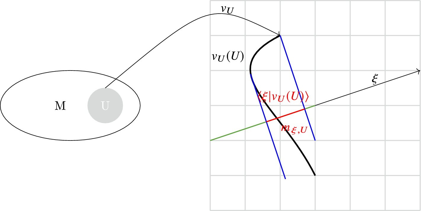
The proof of this theorem uses a Fourier transform and relies on methods of differential geometry; in particular, the normal form of submersions. We can see that the push forward measures
$m_{\xi ,U} :=((\mu _{\pi })_{\vert U})_{{<} \xi \vert v_U(\cdot ){>} }$
 (see Figure 1) are absolutely continuous and verify the Riemann–Lebesgue lemma. This last property, in other words, Rajchman property is enough to get Keplerian shear, it is even an equivalence. We have successfully abstracted this property and obtained the Keplerian shear under the Rajchman property. Using tools from measure theory (conditional expectation) allows to some extent to get rid of the regularity of the velocity. The next theorem is the main result in the continuous case and refers to the real Rajchman property.
Theorem 4.2. (The main result)
Let
$(\Omega , \mu , (g_t)_{t\in \mathbb {R}})$
 be a compatible flow with a compatible measure on a tori bundle as in §2.3.
The dynamical system exhibits Keplerian shear if and only if for all charts
$U\in \mathcal{A}$
 , for all non-zero
$\xi \in \mathbb {Z}^d$
 , the push forward measures
$(m_{\xi ,U})_{\vert \mathbb {R}^*}$
 are Rajchman.
Push forward of measure
${((\mu )_{\pi })}_{\vert U}$
 on
$\mathbb {R}$
 by
${<} \xi \vert v_U{>} $
 (color online).

Proof. Let us prove the direct implication. Let
$U\in \mathcal{A}$
 and non-zero
$\xi \in \mathbb {Z}^d$
 . Take

We have, thanks to the compatibility of
$\mu $
 ,

by push forward theorem. Moreover, with Keplerian shear,

because by Birkhoff’s ergodic theorem,

So,
$(m_{\xi ,U})_{\vert \mathbb {R}^*}$
 is Rajchman.
Let us prove the reciprocal implication. Let
$(U_i)_{i\in I}\in \mathcal{A}^I$
 be a countable partition of M modulo
$\mu _{\pi }$
 . Let

Let
$(i,j)\in I^2,(a_1,a_2)\in \mathbb {L}^\infty _\mu (U_i)\times \mathbb {L}^\infty _\mu (U_j)$
 and
$(\xi _1,\xi _2)\in (\mathbb {Z}^d)^2.$
 Take

for
$l\in \{1,2\}$
 . When
$i\ne j$
 , the supports are disjoint and, in this case,

The same happens when
$\xi _1\ne \xi _2$
 by periodicity of complex exponentials. Finally, when
$\xi _1=\xi _2=0$
 ,
$\mathbb {E}_\mu (\mathrm{Cov}_t(f_1,f_2\vert \mathcal{I}))$
 is constant.
Suppose without loss of generality that
$i=j$
 and
$\xi _1=\xi _2=\xi \ne 0.$
 Set
$W^{\xi }_i=U_i\setminus {({<} \xi \vert v_{U_i}{>} =0)}$
 . We have

because
$(m_{\xi ,U_i})_{\vert \mathbb {R}^*}$
 is Rajchman and thus converges weakly-
$*$
 according to Lemma 2.4.
Moreover,

By [Reference ThomineTho, Proposition 2.4], we have that

We obtain by totality of Y that for all
$f_1,f_2\in \mathbb {L}^2_\mu (\Omega )$
 ,

Remark 4.3. We can also note that the result generalizes to infinite dimensional tori bundles
$\mathbb {T}^{\mathbb {N}}$
 with product topology.
Remark 4.4. When Keplerian shear property holds, the decomposition of Radon–Nikodym–Lebesgue of the image measures
$m_{\xi ,U}$
 in Theorem 4.2 reads as
$(m_{\xi ,U})_{ac}+(m_{\xi ,U})_{sc}+(m_{\xi ,U})_{d}$
 with
$(m_{\xi ,U})_{d}=\alpha \delta _0 $
 , and
$\alpha \geq 0$
 . Recall that the absolutely continuous part satisfies the Rajchman property. The discrete part is concentrated on
$0$
 because otherwise, a non-trivial periodicity would break the Keplerian shear. The behavior of the singular part
$\nu $
 is not obvious, since it may be Rajchman or not, see §2.2.4.
Remark 4.5. When all the
$m_{\xi ,U}$
 are of the form
$(m_{\xi ,U})_{ac}+\alpha _\xi \delta _0$
 , Theorem 4.2 immediately gives Keplerian shear.
4.1 Invariant functions and
$\sigma $
-algebra

Under the conditions of Theorem 4.1, in the regular case, the invariant
$\sigma $
 -algebra is just
$\pi ^{-1}(\mathcal{B}(M))$
 modulo zero measure set. On the functional aspect, it amounts to say that a measurable function f is invariant by the flow if and only if it is
$\mu $
 -a.s. independent on the second variable on every chart U. However, we will first highlight the invariant functions and then the
$\sigma $
 -algebra of invariant sets to compare with the regular case mentioned above. In the following theorem, we will use the Fourier series to identify a characterization of invariance by an orthogonality property.
Proposition 4.6. (Orthogonality and Fourier characterization of invariant functions)
Under the conditions of Theorem 4.2, a function
$f\in \mathbb {L}^2_\mu (\Omega )$
 is invariant according to
$(g_t)_{t\in \mathbb {R}}$
 if and only if for all
$U\in \mathcal{A}$
 , there exists
$ (a_k)_{k\in \mathbb {Z}^d}\in \mathbb {L}^2_{(\mu _{\pi })_{\vert U}}(U)^{\mathbb {Z}^d}$
 such that
$(\mu _{\pi })_{\vert U}\otimes \unicode{x3bb} \text {-}a.e. \,(x,y)\in U\times \mathbb {T}^d$
 ,

In other words, for a chart
$U\in \mathcal{A}$
 and for
$x\in U$
 fixed, non-zero Fourier coefficients have indices orthogonal with the vector
$v_U(x)$
 .
Proof. Let
$f\in \mathbb {L}^2_\mu (\Omega )$
 . Let us start with the direct implication. Suppose that for all
$t\in \mathbb {R}$
 ,

Let
$U\in \mathcal{A}$
 ,
$t\in \mathbb {R}$
 , and
$(x,y)\in U\times \mathbb {T}^d$
 . Since

we have

By Fourier series decomposition, this gives

Hence, by uniqueness of Fourier series coefficients, for all
$k\in \mathbb {Z}^d$
 ,

When k is such that
$\widehat {f\circ \psi _U(x,\cdot )}(k)\ne 0$
 , we get that for all
$t\in \mathbb {R}, t{<} k\vert v_U(x){>} \in \mathbb {Z}$
 . So,
${<} k\vert v_U(x){>} =0$
 and then
$k\in \{v_U(x)\}^\perp $
 . Hence,

Let us see the reciprocal implication. Let
$t\in \mathbb {R}$
 . Suppose that f satisfies for all charts
$U\in \mathcal{A}$
 ,

Let
$z\in \Omega $
 and take
$ U\in \mathcal{A}$
 such that
$z\in \pi ^{-1}(U)$
 . We have

Thus,

by orthogonality. Hence,

Remark 4.7. As a byproduct, the proposition gives an explicit form to the conditional expectation, with respect to the invariant
$\sigma $
 -algebra, of a function
$f\in \mathbb {L}^2_\mu (\Omega )$
 locally by the next formula for
$U\in \mathcal{A}$
 ,
$(\mu _{\pi })_{\vert U}\otimes \unicode{x3bb} \text {-a.e.}\, (x,y)\in U\times \mathbb {T}^d$
 ,

We obviously have
$\pi ^{-1}(\mathcal{B}(M))\subset \mathcal{I}$
 the invariant
$\sigma $
 -algebra; however, the inclusion is generally strict as shown in the following example.
Example 4.8. Consider
$g_t =\mathrm{Id}_{\mathbb {T}^2}$
 ,
$\Omega =\mathbb {T}^2$
 ,
$M=\mathbb {T}$
 .
Clearly,
$\mathcal{I}=\mathcal{B}(\mathbb {T}^2)$
 , while
$\pi ^{-1}(\mathcal{B}(\mathbb {T}))=\{A\times \mathbb {T}\in \mathcal{B}(\mathbb {T}^2) : A\in \mathcal{B}(\mathbb {T})\}\subsetneq \mathcal{I}$
 .
Proposition 4.9. The invariant
$\sigma $
 -algebra is

where for
$U\in \mathcal{A}$
 , the local invariant
$\sigma $
 -algebra on U is

Proof. We prove the direct inclusion. Let
$A\in \mathcal{I}$
 . Let
$U\in \mathcal{A}$
 and set
$C=\psi _U(A\cap \pi ^{-1}(U))$
 . By Proposition 4.6,

which shows that
$C\in \mathcal{I}_U$
 . Hence,
$A\cap \pi ^{-1}(U)\in \psi _U^{-1}(\mathcal{I}_U)$
 and, finally,

Now, we prove the reciprocal inclusion.
Let
$A\in \mathcal{B}(\Omega )$
 such that
$\text { there exists } (B_U)_{U\in \mathcal{A}}\in {{\prod _{U\in \mathcal{A}}}} \psi _U^{-1}(\mathcal{I}_U),\ A= {\bigcup _{U\in \mathcal{A}}} B_U$
 . Then, for all
$t\in \mathbb {R}$
 ,

Let
$U\in \mathcal{A}$
 . By bijectivity of
$\psi _U$
 ,
$\psi _U(B_U)\in \mathcal{I}_U$
 . Hence,

which proves that
$A\in \mathcal{I}$
 by Proposition 4.6.
Remark 4.10. We can see that local invariant sets
$A\in \mathcal{I}_U$
 satisfy

4.2 Convergence speed with the real Rajchman property
We are now interested in the speed of convergence of the conditional correlations. The next result shows that even in
$C^\infty $
 regularity, the order of convergence is limited by the Rajchman order.
Proposition 4.11. (Speed roof)
Let
$0\neq \xi \in \mathbb {Z}^d$
 and
$U\in \mathcal{A}$
 . For all
$\gamma>r((m_{\xi ,U})_{\vert \mathbb {R}^*})$
 , there exists
$(f_1,f_2)\in (\mathcal{C}^\infty ( {\pi }^{-1} (U))\cap \mathbb {L}^2_\mu (\Omega ))^2$
 such that the decay of conditional correlations is not faster than
$t^{-\gamma }$
 , that is, there exists
$C>0$
 such that

Proof. Let
$U\in \mathcal{A}$
 ,
$\xi \in \mathbb {Z}^d\setminus \{0\}$
 . Let
$\gamma>r((m_{\xi ,U})_{\vert \mathbb {R}^*})$
 . Consider

We get

By optimality of
$r((m_{\xi ,U})_{\vert \mathbb {R}^*})$
 , for all
$C>0$
 , for all
$T>0$
 , there exists
$t>T$
 such that

The result follows by definition of conditional correlations.
Remark 4.12. When
$\Omega \simeq M\times \mathbb {T}^d$
 , we can take
$f_1,f_2$
 globally defined of class
$\mathcal{C}^\infty $
 in the Proposition 4.11.
4.3 Speed of decay of conditional correlations for absolutely continuous measures
We assume that
$\Omega =M\times \mathbb {T}^d$
 is the trivial bundle, endowed with an absolutely continuous measure. The speed of decay will depend on the regularity properties of the velocity vector v. We will use the stationary phase method [Reference ZworskiZwo] that allows us to evaluate in an optimal way oscillating integrals. The regularity of the velocity vector and the presence of critical points influences the convergence order.
Before this study, we recall that by an immediate consequence of the Morse lemma, the set of critical points of the velocity vector is discrete.
Lemma 4.13. (Isolation of non-degenerate critical points)
Let M be a finite dimensional
$\mathcal{C}^2$
 manifold and
$v\in \mathcal{C}^2(M,\mathbb {R})$
 . Then, every non-degenerate critical point of v is isolated.
Theorem 4.14. (Stationary phase, e.g. [Reference ZworskiZwo])
Let
$\varphi \in \mathcal{C}^2(\mathbb {R}^n,\mathbb {R})$
 with a unique critical point
$x_c$
 . We suppose that
$x_c$
 is non-degenerate, in other words,
$\det (\mathrm{Hess}(x_c))\ne 0$
 .
Therefore, for any
$a\in \mathcal{C}^1_0(\mathbb {R}^n,\mathbb {R})$
 , for all
$t>0$
 ,

In the following, we say that a is a critical point of order q of a function f if for
$1\le m\le q$
 ,
$f^{(m)}(a)=0$
 and
$f^{(q+1)}(a)\neq 0$
 .
We recall that for a probability measure
$\mathbb {P}$
 , we note
$\widehat {\mathbb {P}}$
 its characteristic function.
Lemma 4.15. (Convergence order with singular points in dimension
$(1,d)$
with
$d\geq 2$
)


Suppose that
$\dim (M)=1\le d$
 and M is a compact manifold of class
$\mathcal{C}^\infty $
 .
Let
$\xi \ne 0_{\mathbb {Z}^d}$
 and
$\ell \ge 2$
 .
We suppose that v is of class
$\mathcal{C}^{\ell }$
 , that there exists a unique critical point of order
$\ell -1$
 for the function
${<} \xi \vert v(\cdot ){>} $
 , and that all the other critical points are of strictly smaller order.
We have

Proof. Here, M is compact Hausdorff, so the number of critical points for each function
${<} \xi \vert v{>} $
 is finite. Let
$(a_k)_{k\in {[\![} 1,m{]\!]} }$
 be the family of critical point of
${<} \xi \vert v(\cdot ){>} $
 with respective orders
$l_k-1\geq 1$
 ,
$1\leq m<l_k,$


Let
$(U_k)_{k\in {[\![} 1,m{]\!]} }$
 be charts such that for all
$k\in {[\![} 1,m{]\!]} $
 ,
$a_k\in U_k$
 . We have

with
$h : \mathbb {R}\to \mathbb {R}\, \mathcal{C}^1$
 such that
$h(x)\xrightarrow [x\to 0]{}h(0)=0.$
 Let us pose for
$k\in {[\![} 1,m{]\!]} ,$


Therefore,

with
$\kappa _k(x)={h^{\prime }(x)}/{l_k({<} \xi \vert v^{(l)}(a_k){>} +h(x))^{({l_k-1})/{l_k}}}$
 . Applying (4.4) to
$x=\varphi _{U_k}(a_k)$
 ,

We get a local inverse of
$w_k$
 on a neighborhood
$W_k$
 of
$0$
 . Let
$(V_k)_{k\in {[\![} 1,m+m^{\prime }{]\!]} }$
 be a family of charts on M such that, for all
$k\in {[\![} 1,m{]\!]} $
 ,

Let
$(\psi _k)_{k\in {[\![} 1,m+m^{\prime }{]\!]} }$
 be a partition of unity subordinated to
$(V_k)_{k\in {[\![} 1,m+m^{\prime }{]\!]} }$
 . We get immediately that for
$k\in {[\![} 1,m{]\!]} $
 ,
$\psi _k(a_k)=1$
 . By inverse function theorem, for
$k\in {[\![} 1,m{]\!]} $
 , we get that on
$W_k$
 , for all
$x\in W_k$
 ,

Writing
$\check {\unicode{x3bb} }$
 as the push forward measure by charts of Lebesgue measure on the manifold M, for
$k\in {[\![} 1,m{]\!]} $
 , we get

with

and
$J(f)(x)$
 denotes the Jacobian of the function f at the point x. We know that
$\check {\psi _k}$
 is subordinated to
$(V_j)_{j\in {[\![} 1,m+m^{\prime }{]\!]} }$
 . Moreover, by (4.5), the support of
$\check {\psi _k}$
 is included in
$U_k$
 . Thus, by (4.7), for all
$t\ne 0$
 ,

Integrating by parts
$u(x)v^{\prime }(x)$
 with
$u(x)=({\check {\psi _k}({x}/{t^{{1}/{l_k}}})}/({2il_k\pi x^{l_k-1}}))$
 and
$v(x)=e^{2i\pi x^{l_k}}-1$
 ,

We know that for all
$\alpha>0,$


Using the development at
$x=0$
 of
$x\in \mathbb {R}\mapsto ({(e^{2i\pi x^{l_k}}-1)}/{x^{l_k-1}})$
 , we get that

For all
$t\ne 0$
 such that
$ \vert t\vert>1$
 , by (4.8), for all
$\alpha>0$
 ,

Thus, by (4.8), there exists
$C_4>0$
 such that for all
$x\in \mathbb {R}$
 , for all
$t\ne 0$
 ,

By Lebesgue convergence theorem,(4.9), (4.10), and (4.11),

For
$k\in {[\![} m+1,m+m^{\prime }{]\!]} ,$
 by Green’s theorem, we get

Thus,

with
$I_{l} :=({1}/({2i\pi l}))\int _{\mathbb {R}} (({e^{2i\pi x^{l}}-1})/{x^{l}})\, d\unicode{x3bb} (x).$
 A simple analysis shows that
$I_l$
 does not vanish. (For l even,
$I_l\in (-\infty ,0)$
 trivially, while for l odd, we have
$I_l\in i(0,\infty )$
 , using a decomposition of the integral on intervals
$[2n,2n+2]$
 .)
By hypothesis, there exists just one critical a point with maximal order
$\ell $
 ; hence,

Thus,

We then get the following proposition.
Proposition 4.16. Under the hypothesis of Lemma 4.15, we get that the order of decay of correlation
$\gamma $
 with
$f_1,f_2\in \mathcal{C}^\infty (\Omega )$
 satisfies

Proof. In the proof of Lemma 4.15, you can take
$f_1=e^{2i\pi {<} \xi \vert v(\cdot ){>} }$
 and
$f_2 = \psi _j$
 with j the index of the chart containing the critical point a with a maximal order
$\ell $
 .
We can now treat the general case.
The following lemma is obtained with [Reference Arnold, Gusein-Zade and VarchenkoAGZV, Theorem 7.5, p. 226].
Lemma 4.17. (Convergence order around a singular point with analytic functions)
We will use the notation and results of [Reference Arnold, Gusein-Zade and VarchenkoAGZV].
We place ourselves in
$\mathbb {R}^n$
 .
Let
$\xi \ne 0_{\mathbb {Z}^d}$
 .
Let v be such that
${<} \xi \vert v{>} $
 is analytic with
$0$
 a critical point of multiplicity
$m\in \mathbb {N}^*$
 .
Then, there exist
$\alpha \in \mathbb {Q}^*_+$
 and
$j\in \mathbb {N}$
 in a compact neighborhood V of
$0$
 such that for all
$\varphi \in \mathcal{D}_V(\Omega )$
 ,

Definition 4.1. (Logarithmic convergence order)
Consider a probability measure
$\nu $
 on
$(\mathbb {R},\mathcal{B}(\mathbb {R}))$
 .
We call the logarithmic convergence order of
$\nu $
 the value

The next result may be obtained by a partition of unity and the previous lemma.
Proposition 4.18. (Convergence order with singular points in dimension
$(n,d)$
with
$d\geq 2$
)


Suppose that M is analytic. Let
$\xi \ne 0_{\mathbb {Z}^d}$
 . Suppose that v is such that
${<} \xi \vert v{>} $
 is analytic. We have that

Corollary 4.19. Let v be a
$\mathcal{C}^2$
 function. If there exists only one critical point
$a\in M$
 and it satisfies

then
$r(\unicode{x3bb} _{{<} \xi \vert v(\cdot ){>} })= {n}/{2}.$

Proof. Let
$\xi \ne 0_{\mathbb {Z}^d}$
 . Applying the stationary phase theorem on respective charts
$(U,\varphi _U)$
 of
$\mathcal{A}$
 containing at most just one critical point
$a\in U$
 and test functions
$\psi $
 on U, we get

By partition of unity, we obtain

Remark 4.20. Note that the result is consistent with the case
$n=1$
 .
We recall the definition of Thomine [Reference ThomineTho].
Definition 4.2. (Anisotropic Sobolev space on
$\mathbb {R}{\kern-1pt}\times{\kern-1pt} \mathbb {T}$
)

Let
$s{\kern-1pt}\geq{\kern-1pt} 0$
 . Let
$h : x{\kern-1pt}\in{\kern-1pt} \mathbb {R}{\kern-1pt}\mapsto{\kern-1pt} \sqrt {1+x^2}$
 . Let

Proposition 4.21. Consider
$(\mathbb {R}\times \mathbb {T},\mu \otimes \unicode{x3bb} ,(g_t)_{t\in \mathbb {R}})$
 such that
$r=r(\mu )>0$
 and for
$(x,y)\in \mathbb {R}\times \mathbb {T},g_t(x,y)=(x,y+tx)$
 . Let
$s>\tfrac 12$
 . For
$\varepsilon \in\ ]0,{1}/{2s}[,$
 let
$q_\varepsilon := \min {\{s(1-\varepsilon ),r(\mu )\}}$
 . Then, we get for all
$\varepsilon \in\ ]0,{1}/{2s}[$
 , there exists
$C_{s,\varepsilon }>0$
 such that for all
$t>0$
 ,

and if
$\gamma>0$
 denotes the convergence order on
$H^{s,0}(\mathbb {R}{\kern-1pt}\times{\kern-1pt} \mathbb {T})$
 , we get
$\min {\{s{\kern-1pt}-{\kern-1pt}\tfrac 12,r(\mu )\}}{\kern-1pt}\leq{\kern-1pt} \gamma $
 . Moreover, if
$\mathrm{supp}(\mu )$
 is compact, then
$\gamma \leq r(\mu )$
 .
Proof. Let
$s>\tfrac 12$
 and
$(f_1,f_2)\in (H^{s,0}(\mathbb {R}\times \mathbb {T}))^2$
 . Then, by Cauchy–Schwarz inequality and Parseval,

with

We can consider
$k{\kern-1pt}={\kern-1pt}1$
 considering
$kt$
 instead of t. Let
$D_1(t) {\kern-1pt}:={\kern-1pt} \{(u,v){\kern-1pt}\in{\kern-1pt} \mathbb {R}^2 : \vert t-(u-v)\vert \leq 2t \text { and } \vert v\vert \leq ({t}/{4})\}$
 ,
$D_2(t) := \{(u,v)\in \mathbb {R}^2 : \vert t-(u-v)\vert \leq 2t\text { and } \vert v\vert>({t}/{4})\}$
 , and
$D_3(t) :=\{(u,v)\in \mathbb {R}^2 : \vert t-(u-v)\vert> 2t\}$
 .
We get that for
$(u,v)\in D_1(t)$
 ,

and for
$(u,v)\in D_2(t)$
 ,

Using that
$s>\tfrac 12$
 , for all
$\varepsilon \in\ ]0,{1}/{2s}[$
 ,

and by (4.13) and (4.14), and for


Therefore, by definition of
$D_3(t)$
 , (4.16), and (4.17),

with
$D_{s,\varepsilon } = \max {\{{1}/({2^{r(\mu )}}),{4}^{s(1-\varepsilon )}\sqrt {2}\}}$
 and
$q_\varepsilon =\min {\{r(\mu ),s(1-\varepsilon )\}}$
 . Thus,

By (4.12), (4.15), and (4.19),

Moreover, for
$\gamma>0$
 , the convergence order on
$H^{s,0}(\mathbb {R}{\kern-1pt}\times{\kern-1pt} \mathbb {T})$
 , we get
${\min {\{s{\kern-1pt}-{\kern-1pt}\tfrac 12,r(\mu )\}}{\kern-1pt}\leq{\kern-1pt} \gamma }$
 and when
$\mathrm{supp}(\mu )$
 is compact,
$\gamma \leq r(\mu )$
 .
Remark 4.22. When
$(f_1,f_2)\in (H^{s,0}(\mathbb {R}\times \mathbb {T}))^2$
 with
$s\geq (({r(\mu )+1})/{2})$
 , we get that
$\gamma =r(\mu )$
 as the optimal order of convergence when
$\mathrm{supp}(\mu )$
 is compact.
Remark 4.23. For
$s>\tfrac 12$
 , for all integer
$k>s+\tfrac 32$
 ,
$\mathcal{C}^k_c(\mathbb {R}\times \mathbb {T})\subset H^{s,0}(\mathbb {R}\times \mathbb {T})$
 , and then, for
$k>s+\tfrac 32$
 , the convergence order
$\gamma>0$
 for
$\mathcal{C}^k_c(\mathbb {R}\times \mathbb {T})$
 is such that
$\gamma \in [\min {\{s-\tfrac 12,r(\mu )\}},r(\mu )]$
 when
$\mathrm{supp}(\mu )$
 is compact.
Remark 4.24. When
$\mu =\unicode{x3bb} _v$
 with
$v\in \mathcal{C}^\infty $
 with a unique critical point of order
$l-1$
 with
$l\geq 3$
 , then
$\gamma =r(\mu )={1}/{l}$
 .
5 Keplerian shear, Rajchman property, and Diophantine approximation
In this section, we present an application of Keplerian shear (with speed estimates) to dynamical Borel–Cantelli lemmas. The latter is linked to Diophantine approximation and we discuss the relations between the Rajchman property and Diophantine properties.
Let
$(\Omega ,\mu ,T)$
 be a measure preserving dynamical system. For a sequence of measurable sets
$(A_n)$
 , the aim of the dynamical Borel–Cantelli lemma is to assert that the events
$T^n(x)\in A_n$
 appear infinitely often almost surely, if and only if
$\sum \mu (A_n)=+\infty $
 . The independence condition of the classical (non-dynamical) case is replaced by some decorrelation condition (see e.g. [Reference Chernov and KleinbockCK2]).
Our main application consists here in readjusting the dynamical Borel–Cantelli lemma in the non-ergodic case. We provide an adaptation of Sprindzuk’s theorem inspired by the thesis of Xing [Reference XingXin]. The Keplerian shear will ensure that for almost any x, there exists an infinity of integers n satisfying
$T^n(x)\in A_n$
 , where the measurable set
$A_n$
 is a shrinking target. The dynamical Borel–Cantelli lemma allows us to study the behavior of the sum
$\sum _{k=0}^N\mathbb {1}_{A_k}\circ T^k$
 using the Keplerian shear.
Theorem 5.1. (Variable Sprindzuk)
Let
$(f_k)_{k\in \mathbb {N}^*}$
 and
$(g_k)_{k\in \mathbb {N}^*}$
 be two sequences of measurable and non-negative functions. Let
$(\varphi _k)_{k\in \mathbb {N}^*}$
 be a real sequence such that for all
$k\in \mathbb {N}^*$
 ,
$0\leq g_k\leq \varphi _k\leq 1\,\mu $
 -almost everywhere. Let
$\delta>1$
 and
$C>0$
 . Suppose that for all
$(m,n)\in (\mathbb {N}^*)^2$
 satisfying
$n\geq m$
 ,

Then, for all
$n\in \mathbb {N},$
 for all
$\varepsilon>0$
 ,

with
$\phi (n)= \sum _{k=1}^n\varphi _k$
 .
For the proof, we will elaborate on the proof of the original theorem in the book by Sprindzuk [Reference Sprindzuk, Silverman and WinstonSpr, (68), p. 45].
Proof. Let
$\delta>1$
 and let us denote for
$I\subset \mathbb {N}^*,\phi (I)=\sum _{k\in I}\varphi _k$
 . By the fact that for all
$ k\in \mathbb {N}^*$
 ,
$0\leq \varphi _k\leq 1$
 , we have that there exists
$(n_v)_{v\in \mathbb {N}^*}\in {\mathbb {N}^*}^{\mathbb {N}^*}$
 such that for all
$v\in \mathbb {N}^*$
 ,

We have also for all
$v\in \mathbb {N}^*$
 ,

and for all
$v\in \mathbb {N}^*$
 ,

Thus, for all
$u,v\in \mathbb {N}^*$
 ,

Let

Let for
$r\in \mathbb {N}^*, s\in {[\![} 0,r{]\!]} $
 sets of parts,

Let
$r\in \mathbb {N}^*$
 and
$s\in {[\![} 0,r{]\!]} .$
 We notice that

Let
$i\in {[\![} 0,2^{r-s}-1{]\!]} .$
 We have that

Therefore,

and

Thus,

Therefore,

Denote

Thus, we have

Let

Therefore,

for some constant
$C_1$
 . Let
$\varepsilon>0$
 . By the Markov inequality,

By the Borel–Cantelli lemma,

For
$v\in \mathbb {N}^*$
 , we have that
${[\![} 1,v{]\!]} $
 can be aligned into a finite number
$r_v$
 of intervals
$J_r$
 such that

Let
$J(v)$
 denote the set of these intervals. We then get

By the Cauchy–Schwarz inequality,

Thus,

Therefore,

Let
$n\in \mathbb {N}^*.$
 Taking
$v\in \mathbb {N}^*$
 such that
$n_v\leq n\leq n_{v+1}$
 , we get

Moreover,

In addition,

Then,

and

Therefore,

Theorem 5.2. (Dynamical Borel–Cantelli lemma by Keplerian shear)
Suppose that
$(\Omega ,T,\mu )$
 is a discrete measure preserving dynamical system with Keplerian shear. Let
$(A_n)$
 be a sequence of measurable sets and note
$S_{M,N} = \sum _{k=M}^N\mathbb {1}_{A_k}\circ T^k$
 ,
$S_N=S_{0,N}$
 .
We suppose that Condition (1a) or (1b) holds and so does Condition (2).
-
(1)
-
(a) There exists $\gamma>0,C>0$
such that for all
$(j,k)\in \mathbb {N}^2$
satisfying
$k\ne j$
, $$ \begin{align*} \vert \mathbb{E}(\mathrm{Cov}_{k-j}(\mathbb{1}_{A_j},\mathbb{1}_{A_k}\vert\mathcal{I}))\vert \leq \frac{C}{ \vert k-j\vert^\gamma}.\end{align*} $$
-
(b) There exists $\gamma>0,D>0$
, and
$\mathcal{B}\subset \mathbb {L}^2_\mu (\Omega )$
, a Banach space such that there exists
$C>0$
such that for all
$f,g\in \mathcal{B}$
, for all
$n\in \mathbb {N}$
,
$\vert \mathbb {E}(\mathrm{Cov}_n(f,g\vert \mathcal{I}))\vert \leq (({C\Vert f\Vert _{\mathcal{B}}\Vert g\Vert _{\mathcal{B}}})/{n^{\gamma }})$
and for all
$j\in \mathbb {N}$
,
$\Vert \mathbb {1}_{A_j}\Vert _{\mathcal{B}}\leq D$
.
-
-
(2) There exists $\beta>\max (\frac 12,1-\gamma /2)$
such that
$\liminf _{N\to \infty }({{\mathbb {E}(S_N\vert \mathcal{I})}/{N^\beta }})>0\ \mu \text {-}a.s$
.


We have

Remark 5.3. We emphasize that in contrast to usual dynamical Borel–Cantelli lemmas, the evolution of the sum
$S_N$
 is only compared with the conditional expectation
$\mathbb {E}(S_N\vert \mathcal{I})$
 , instead of the classical expectation
$E(S_N)$
 .
Proof. Without loss of generality, we assume that
$\gamma \in (0,1)$
 . Note that Condition (1b) implies Condition (1a), so Condition (1a) holds in both cases.
By expansion of the square as a double sum and the series-integral comparison criterion, we get
$\text { for all } (M,N)\in \mathbb {N}^2$
 such that
$M<N$
 ,

By setting
$\delta = 2-\gamma $
 and noticing that
$E(S_{M,N})\le N-M$
 , we get that there exists
$D>0$
 satisfying

By variable Sprindzuk Theorem 5.1 with
$\varphi _k=1$
 for all k, we get

Then,

Example 5.4. Let us place ourselves in the case of
$(\mathbb {T}^2,\unicode{x3bb} \otimes \unicode{x3bb} ,T)$
 with

Consider a sequence
$(b_n)\in \mathbb {T}^{\mathbb {N}}$
 and let

with
$0<p<\tfrac 12.$
 We get that
$\text { for all } N\in \mathbb {N}^*$
 ,

Let
$s:=\frac 12$
 and
$n\in \mathbb {N}^*$
 . By direct computation of the Fourier coefficients of
$1_{A_n}$
 , we see that

since

By the decorrelation estimates in [Reference ThomineTho],
$\text { for all } (k,j)\in \mathbb {N}^2$
 ,

The hypotheses are then brought together, applying Theorem 5.2 with
$\gamma =1$
 and
${\beta \in (\frac 12,1-p)}$
 , so we get

In the case of any measure of Rajchman, we have as an application a proposition based on a work of Athreya [Reference AthreyaAth, Theorem 4.2, p. 551] and also the theorem of Kurzweil [Reference KurzweilKur] and [Reference TsengTse, Theorem 1.3, p. 3] concerning Diophantine numbers. To introduce this theorem, we will also have to recall the shrinking target property (STP) and its monotone version (MSTP) of a dynamical system.
Definition 5.1. (Shrinking target properties)
A discrete dynamical system
$(\Omega ,\mu ,T)$
 is called STP if for all sequences of balls
$(B_n)_{n\in \mathbb {N}}$
 of radius
$r_n>0$
 tending to
$0$
 and satisfying

The MSTP property is defined in the same way, assuming in addition that the sequence
$r_n$
 is monotone.
Definition 5.2. (s-Shrinking target properties)
A discrete dynamical system
$(\Omega ,\mu ,T)$
 is called STP if for all sequences of balls
$(B_n)_{n\in \mathbb {N}}$
 of radius
$r_n>0$
 tending to
$0$
 and satisfying

The s-MSTP property is defined in the same way, assuming in addition that the sequence
$r_n$
 is monotone.
Let us now recall Kurzweil’s theorem in dimension
$1$
 .
Theorem 5.5. (Kurzweil and Tseng)
Consider the dynamical system
$(\mathbb {T},\unicode{x3bb} ,T_\alpha )$
 with
$\alpha \in \mathbb {T}$
 and
$ T_\alpha : x\mapsto x+\alpha $
 . Then, the dynamical system is s-MSTP if and only if
$\alpha $
 is s-Diophantine (that is,
$\alpha \in \mathcal{D}\mathrm{io}(s)$
 , see Definition 2.9).
We also deduce with the work of Chaika and Constantine [Reference Chaika and ConstantineCK] the following theorem.
Theorem 5.6. (Kurzweil)
For
$\unicode{x3bb} \text {-}a.e. \,\alpha \in [0,1[, (\mathbb {T},\unicode{x3bb} , T_\alpha )\, is \, \textit{MSTP}$
 .
In the case of singular continuous Rajchman measures, we will have a weakening of Theorem 5.6 of Kurzweil. First, we present a dynamical Borel–Cantelli lemma for Rajchman measures. As in Theorem 5.2, it is based on covariance estimates. Here, they do not rely on the Keplerian shear but are obtained directly from the Rajchman property.
Theorem 5.7. (Dynamical Borel–Cantelli lemma for Rajchman measures)
Consider a Rajchman measure
$\mu $
 on
$\mathbb {T}$
 of order
$0\le r(\mu )\le \tfrac 12$
 . Let T be the transvection on
$\mathbb {T}^2$
 defined by
$T(x,y)=(x,x+y)$
 . Let
$C>0$
 and
$s>({1}/({r(\mu )}))-1$
 . We have

where

Proof. Let
$p={1}/{s}$
 . Let for
$(m,n)\in (\mathbb {N}^*)^2$
 such that
$m>n$
 the sum

By definition and using the invariance of the measure, we get

Using the Fourier series of the indicator function of an interval, we obtain

Combining this upper bound with the previous estimate gives

Let
$\delta =2-r(\mu )-p(1+r(\mu ))$
 . Since
$p<({r(\mu )}/({1-r(\mu )}))$
 , we have
$({\delta }/{2})<1-p$
 . Therefore, by Sprindzuk’s theorem,

Hence,

Remark 5.8. We observe that this ‘loss of power’ in the Borel–Cantelli lemma above increases as the Rajchman order decreases.
The next result relates the order of a Rajchman measure to Diophantine properties of its support and, thus, the MSTP property. This result will therefore also show Proposition 2.7.
Proposition 5.9. (General Kurzweil for Rajchman measures)
Consider a Rajchman measure
$\mu $
 on
$\mathbb {T}$
 of order
$0\le r(\mu )\le \tfrac 12$
 . Let
$s>({1}/({r(\mu )}))-1$
 . We have
$\mu (\mathcal{D}\mathrm{io}(s))=1$
 , or equivalently,

Proof. Let
$C>0$
 . For
$n\in \mathbb {N}^*$
 , set
$A_n=\ ]({p}/{n})-({C}/{n^{s+1}}),({p}/{n})+({C}/{n^{s+1}})[$
 . Using an elementary computation based on the Fourier series of the indicator function of an interval and the periodicity of the intervals, we get

Take
$\varepsilon $
 and r such that
$1/({s+1})<\varepsilon <r<r(\mu )$
 . Since
$|\!\sin (t)|\le |t|^\varepsilon $
 for all real t, we obtain

Therefore,
$\sum _n\mu (A_n)=+\infty $
 since
$r+s\varepsilon>1$
 . By the Borel–Cantelli lemma,

This proves that
$\mu (\mathcal{D}\mathrm{io}(s))=1$
 . By Kurzweil–Tseng Theorem 5.5,

Recall that when we have
$r(\mu )>\tfrac 12$
 , the measure
$\mu $
 is absolutely continuous and therefore by Kurzweil theorem cited above,
$\mu \text {-almost all}\, \alpha \in [0,1[$
 , the system
$(\mathbb {T},\unicode{x3bb} ,T_{\alpha })$
 is
$1$
 -MSTP.
Remark 5.10. We can note that the result obtained in Proposition 5.9 remains consistent with that obtained with the Keplerian shear in Theorem 5.7 because

Remark 5.11. For a Rajchman measure with positive order
$r(\mu )>0$
 ,
$\mu \text {-}a.e.\, \alpha \in [0,1[$
 is Diophantine, that is,
$\mathrm{Dio}(\alpha )<+\infty \, \mu $
 -almost surely.
The following result shows that Proposition 5.9 is optimal.
Proposition 5.12. (Optimality of the Rajchman order [Reference KaufmanKau])
Let
$0<r< \frac 12$
 . Then, for all
$1<s<({1}/{r})-1$
 , there exists
$\mu $
 a Rajchman measure such that
$r(\mu )=r$
 and
$\mu (\mathcal{D}\mathrm{io}(s))=0$
 .
Proof. Let
$\varepsilon =({1}/{r})-(s+1)>0$
 . We can consider
$\mu _{\alpha }$
 with
$\alpha = s-1+\varepsilon $
 constructed in the document of Kaufman [Reference KaufmanKau] with its support in
$E(\alpha )\subset [0,1]\setminus {\mathcal{D}\mathrm{io}(s)}$
 .
Remark 5.13. With convex combination, for any
$s>1$
 , we can construct a Rajchman measure
$\mu $
 for which
$\mu (\mathcal{D}\mathrm{io}(s))$
 is equal to any value in
$[0,1]$
 .
Example 5.14. (Diophantine property with self-similar measures)
The self-similar measure
$\mu _{\theta }$
 with
$\theta>1$
 not being Pisot, according to the work of Pablo Shmerkin and Kahane [Reference KahaneKah], has an order of Rajchman
$r(\mu _{\theta })>0$
 . In particular,
$\mu _{\theta }\text {-a.e.} \,\alpha \in [0,1]$
 is Diophantine.
Example 5.15. (Liouville property with Rajchman measures on
$S_\infty $
)

The measure of Rajchman
$\mu _{\infty }$
 mentioned in Example 2.9 is Rajchman, but since its support
$S_\infty $
 almost surely contains Liouville numbers, then we deduce by contrapositive of Proposition 5.9 that
$\mu _{\infty }$
 does not have a strictly positive Rajchman order, that is, that
$r(\mu _{\infty })=0$
 .
6 Flow on compact Lie group bundle
In this section, we extend the results on Keplerian shear for tori bundles from §4 to non-abelian bundles. The setting is essentially the same except that we replace the torus with a compact connected Lie group. It is worth mentioning that the core of the proofs will not differ too much. The fundamental reason being that even if the group is not abelian, each individual orbit defines a one-parameter subgroup that is therefore abelian; hence a torus.
6.1 Lie group bundle and compatible flow
Let G be a compact connected Lie group.
Definition 6.1. Let
$(M,\mathcal{A})$
 be a Lindelöf manifold of dimension
$n\in \mathbb {N}^*$
 of class
$\mathcal{C}^1$
 .
Let
$(\Omega ,\mu )$
 be a Borelian space, G a connected compact Lie group, and
$\pi $
 a continuous map from
$\Omega $
 into M.
Then,
$\Omega $
 is a G-bundle if:
-
(1) locally, we have for the charts U of $\mathcal{A}$
a homeomorphism
$\psi _U : \pi ^{-1}(U)\to U\times G$
; -
(2) for all U in $\mathcal{A},\pi _1\circ \psi _U=\pi _{\vert U}.$


To define the continuous flow, we are going to use the exponential defined on the corresponding Lie algebra
$\mathrm{Lie}(G)$
 of the group G. Here, the connectedness and the compactness of the group provide that the exponential
$\exp \colon \mathrm{Lie}(G)\to G$
 is surjective, and injective from a neighborhood of the origin
$B(0,\delta _{\text {inj}})$
 to a neighborhood of the neutral element of e of G. The latter implies that any continuous flow satisfying for all
$y,z\in G, \phi _t(yz)=\phi _t(y)z$
 is of the form
$\phi _t(y)=\exp (tv)y$
 for some
$v\in \mathrm{Lie}(G)$
 . This motivates the notion of compatible flow.
Definition 6.2. (Compatible flow)
Let
$(g_t)_{t\in \mathbb {R}}$
 be a flow on
$(\Omega ,\mu )$
 .
Then,
$(g_t)_{t\in \mathbb {R}}$
 is a compatible flow if and only if:
-
(1) there exists for all $U\in \mathcal{A}$
, a measurable function
$v_U : U\to \mathrm{Lie}(G)$
; -
(2) $\text {for all } U\in \mathcal{A},\text { for all } (x,y)\in U\times G, \psi _U\circ g_t\circ \psi _U^{-1}(x,y)=(x,\exp (tv_U(x))y)$
.


Definition 6.3. (Compatible measure)
Consider the notation previously established with the connected compact Lie group bundle.
Let
$U\in \mathcal{A}$
 . Let us pose
$\mu ^U := \mu _{\psi _U}$
 and
$\mu ^{\prime } := \mu _{\pi }$
 . Then,
$\mu $
 on
$\Omega $
 is compatible if and only if

Next, results by Delzant [Reference DelzantDel] will allow us to transfer the dynamics from G to the torus.
Proposition 6.1. Let G be a compact and connected Lie group.
-
(i) Any compact, connected, and abelian Lie group is isomorphic to a torus.
-
(ii) The group G admits a maximal torus T,
$$ \begin{align*}G={\bigcup_{g\in G}} gTg^{-1}\end{align*} $$and for all maximal torus $T^{\prime }$
, there exists
$g\in G$
such that $$ \begin{align*}T^{\prime}=gTg^{-1}.\end{align*} $$
-
(iii) Any closed subgroup H of G admits a group structure of Lie and $\mathrm{Lie}(H)$
is a linear subspace of
$\mathrm{Lie}(G)$
. -
(iv) The orbital group of a direction $v\in \mathrm{Lie}(G)$
, $$ \begin{align*} H_v :=\overline{\{\exp(tv)\in G : t\in \mathbb{R}\}},\end{align*} $$is an abelian Lie group, compact and connected, and so is isomorphic to a torus.
-
(v) For all $v\in \mathrm{Lie}(G)$
, for all maximal torus T of G, there exists
$g\in G$
such that $$ \begin{align*}H_v\subset gTg^{-1}.\end{align*} $$


Now, we fix T a maximal torus of G and an isomorphism
$\chi : T\to \mathbb {T}^R$
 , where R is the dimension of T.
The combination of these results shows that each individual orbit can be embedded in the same torus T, a situation similar to the case of a tori bundle, which is the setting of §4. More precisely, by Proposition 6.1(v), for
$v\in \mathrm{Lie}(G)$
 , we get a
$g\in G$
 such that
$H_v\subset gTg^{-1}$
 . To exploit this property, we need a measurable selection of the element g, as a function of v.
Let
$h : \mathrm{Lie}(G)\to G$
 be a measurable map such that for all
$v\in \mathrm{Lie}(G)$


(A construction of such a measurable function h is done in §6.4, but other choices are possible.) Let us pose for
$U\in \mathcal{A}$
 and
$x\in U$
 ,

with
$\mathrm{Ad}$
 the adjoint operator defined for
$g\in G$
 and
$v\in \mathrm{Lie}(G)$
 by

Let us pose for non-zero
$\xi \in \mathbb {Z}^d$
 and
$U\in \mathcal{A}$
 ,
$\nu ^{(\xi ,U)}:=\mu ^{\prime }_{\vert U} {{<} \xi \vert w_U(\cdot ){>} }.$

6.2 Keplerian shear and Rajchman measures on G-bundle
Theorem 6.2. The dynamical system
$(\Omega ,\mu ,(g_t)_{t\in \mathbb {R}})$
 exhibits Keplerian shear if and only if for all non-zero
$\xi \in \mathbb {Z}^R$
 , and for all
$U\in \mathcal{A}$
 ,
$\nu ^{(\xi ,U)}_{\vert \mathbb {R}^*}$
 is Rajchman.
The plan of the demonstration will initially be to come back to a situation very similar to that of the torus bundle by relying on the maximal torus. To do this, we are going to use the orbital group
$H_{v_U(x)}$
 that is isomorphic to a torus. The second step will be for a chart
$U\in \mathcal{A}$
 and
$x\in U$
 fixed to conjugate the action of
$\exp (t v_U(x))$
 on G to a translation by
$tw_U( x)$
 on the torus. Once immersed in this configuration provided by Lemma 6.3, we will be able to carry out the same reasoning as in the torus to arrive at the property of Rajchman of
$\nu ^{(\xi ,U)}_{\vert \mathbb {R}^*}$
 .
Consider the neighborhood V of the local coordinate system of the second kind associated with
$\mathrm{Lie}(T)$
 and
$(\mathrm{Lie}(T))^{\perp }$
 .
We cover G with a finite family of elements
$(g_k)_{k\in {[\![} 1,l{]\!]} }\in G^{{[\![} 1,l{]\!]} }$
 such that

Let
$(W_k)_{k\in {[\![} 1,l{]\!]} }$
 such that
$W_1=Vg_1$
 and

Let
$\varphi : G^2\to G$
 be defined by
$\varphi (x,y)=xy$
 and
$\varphi ^v : G^2\to G$
 be defined by
$\varphi ^v(x,y)=\varphi (h(v)x,y)$
 . By [Reference BourbakiBou], we can define

Let
$ \eta : \mathrm{Lie}(G)\times G\to G^2$
 be defined by
$\eta (\theta ,y)=(\exp (\theta ),y)$
 . We define for
$v\in \mathrm{Lie}(G),\, k\in {[\![} 1,l{]\!]} $
 , and
$x\in Vg_k$
 ,


for
$(\theta ,y)\in \mathrm{Lie}(G)\times G$
 and
$t\in \mathbb {R}$
 ,

and for
$z\in G$
 ,

Thus, for all
$k\in {[\![} 1,l{]\!]} $
 , for all
$x\in h(v)Vg_k$
 , we get

Lemma 6.3. Let
$U\in \mathcal{A}$
 and
$(f_1,f_2)\in (\mathbb {L}^2_{\mu ^{\prime }_{\vert U}\otimes \mathcal{H}}(U\times G))^2$
 . We define for
$t\in \mathbb {R}$
 ,

Then,

with

and
$m^{\prime }_{(x,k)}=(\chi _{v_U(x)}\circ \exp )_{*}m_{(x,k)}$
 is the push forward measure obtained by transfer theorem, where
$m_{(x,k)}=(\psi _k^{v_U(x)})_{*} \mathcal{H}$
 is the associated push forward measure. We recall that
$D\chi _{v_U(x)}(e)=D\chi (e)\circ \mathrm{Ad}_{h(v_U(x)).}$

Proof. Let non-zero
$\xi \in \mathbb {Z}^R$
 . Let
$U\in \mathcal{A}$
 and
$(f_1,f_2)\in (\mathbb {L}^2_{\mu ^{\prime }_{\vert U}\otimes \mathcal{H}}(U\times G))^2$
 . We have the following expression for
$b_t(f_1,f_2)$
 :

We have completed the first step by placing ourselves in the Lie algebra of the maximal torus T, which is abelian, so

We are now at the second step placing ourselves in the sections of the Lie group G by T. So,

where the integrand
$I(k,U,x)$
 is equal to

We pass here in the torus isomorphic to T. Since

and

we get

This proves (6.11).
We are then in the case of a torus foliation by the variable x, which will then allow us to apply the same reasoning as in the case of the torus.
Proof of Theorem 6.2.
Let us begin with the direct implication. Suppose that the dynamical system
$(\Omega ,\mu ,(g_t)_{t\in \mathbb {R}})$
 exhibits Keplerian shear. Let
$U\in \mathcal{A}$
 and let

Let
$(f_1,f_2)\in (\mathbb {L}^2_{\mu ^{\prime }_{\vert U} \otimes \mathcal{H}}(U\times G))^2$
 such that

and

taking the notation of Lemma 6.3. Then,

with

Thus, by Lemma 6.3,

By the Keplerian shear property, the right-hand term converges and as in (4.1), the limit is zero. So,

Let us continue with the reciprocal implication. Let R be the dimension of the maximal torus of G.
Consider
$k\in {[\![} 1,l{]\!]} $
 and define the measure
$\omega ^k$
 on
$U\times \mathbb {T}^R\times W_k$
 by

Let
$U\in \mathcal{A}$
 and
$(\xi _1,\xi _2)\in (\mathbb {Z}^R)^2$
 . Let
$(f_1,f_2)\in (\mathbb {L}^2_{\mu ^{\prime }_{\vert U }\otimes \mathcal{H}}(U\times G))^2$
 such that,

and

with
$a_1$
 and
$a_2$
 square summable functions in the appropriate Lebesgue space. If
${m\neq m'}$
 , the scalar product between
$f_1,f_2$
 is zero. Therefore, we assume that
$m=m'$
 . So, by Lemma 6.3,

with

By hypothesis, when
$\xi _1\ne 0$
 ,

Then, by Lemma 2.4, we have that
$\exp (2i\pi t\cdot )$
 converge weakly-
$*$
 in
$\mathbb {L}^{\infty }_{\nu ^{\xi _1,U}}(\mathbb {R})$
 to
$0$
 . Thus,

Then, remembering (6.12), the integral

converges as
$t\rightarrow \pm \infty $
 towards

By totality obtained by the Fourier series expansion, this gives that for all functions
$f_1,f_2\in \mathbb {L}^2_{\mu ^{\prime }_{\vert U}\otimes \mathcal{H}}(U\times G)$
 , the integral

converges as
$t\to \pm \infty $
 towards

6.3 Keplerian shear on G-bundle in the regular case
Now, the aim here is to give an analog of [Reference ThomineTho, Theorem 3.3], which guarantees Keplerian shear for flows with regular velocities and the negligible critical points, for absolutely continuous measures.
Theorem 6.4. If for all
$U\in \mathcal{A}$
 ,
$w_U$
 is
$\mathcal{C}^1$
 ,
$\mu ^{\prime }_{\vert U}\ll \unicode{x3bb} $
 and

then the dynamical system
$(\Omega ,\mu ,(g_t)_{t\in \mathbb {R}})$
 has Keplerian shear.
Lemma 6.5. Let
$V{\kern-1pt}\subset{\kern-1pt} \mathbb {R}^d$
 be an open set and
$f\colon V{\kern-1pt}\to{\kern-1pt} \mathbb {R}$
 a
$\mathcal{C}^1$
 map. If
$\{d_xf{\kern-1pt}={\kern-1pt}0\}\setminus \{f{\kern-1pt}={\kern-1pt}0\}$
 has zero Lebesgue measure, then for any
$a\in \mathbb {R}^*$
 ,
$\{f=a\}$
 has zero Lebesgue measure.
Proof. Let
$(e_i)$
 be the canonical basis of
$\mathbb {R}^d$
 and denote by
$\mathcal{C}_i$
 the cone of vectors
$h\neq 0$
 such that the angle between h and
$e_i$
 is less than or equal to
$\pi /8$
 .
Let
$a\in \mathbb {R}^*$
 , and set
$A=\{f=a\}$
 and
$A^{\prime }$
 the set of Lebesgue density points of A, that is,
$\unicode{x3bb} (A\cap B(x,r))/\unicode{x3bb} (B(x,r))\to 1$
 as
$r\to 0$
 for each
$x\in A^{\prime }$
 .
Suppose that
$x\in A^{\prime }$
 . For each
$i=1,\ldots ,d$
 , there exists a sequence
$h_n^i\in \mathcal{C}_i$
 such that
$x+h_n^i\in A$
 and
$h_n^i\to 0$
 . Without loss of generality, we may assume that
$h_n^i/\|h_n^i\|$
 converges to some
$h^i\in \mathcal{C}_i$
 . Since
$f(x+h_n^i)=a=f(x)$
 , a first-order expansion shows that
$d_xf(h^i)=0$
 . Since the
$h_i$
 form a basis of
$\mathbb {R}^d$
 , this implies that
$d_xf=0$
 .
By assumption, we get that
$A^{\prime }$
 , and therefore A, has zero measure.
Proof of Theorem 6.4.
Let
$U\in \mathcal{A}$
 . Let us show that the measures
$\nu ^{(\xi ,U)}$
 have the Rajchman property.
Let
$\xi \in \mathbb {Z}^d \setminus \{0\}$
 . By Radon–Nikodym,

However,

Thus, by Lemma 6.5,

By local normal form of submersions, we can choose a countable family
$(\varphi _k, V_k)_{k\in \mathbb {N}}$
 of open charts on M which are pairwise disjoints, cover
$U\setminus ({\bigcup _{\xi \in \mathbb {Z}^d \setminus \{0\}}} \{x\in U : d{<} \xi \vert w_U(x){>} =0\})$
 up to a Lebesgue-negligible set, and for all
$k\in \mathbb {N}$
 and all
$x\in \varphi _k(V_k)$
 ,

Therefore, for
$k\in \mathbb {N}$
 ,

However, we have

Thus, by Riemann–Lebesgue,

Therefore,

By Theorem 6.2, we get that
$(\Omega ,\mu ,(g_t)_{t\in \mathbb {R}})$
 exhibits Keplerian shear.
We can develop a corollary of Theorem 6.4. We define

and we assume that
$\bar h$
 is
$\mathcal{C}^1$
 on a full measure open set.
Corollary 6.6. We suppose that for a countable family
$(U_j)_{j\in \mathbb {N}}$
 of charts which cover M up to a Lebesgue-negligible set,
$\bar h$
 is
$\mathcal{C}^1$
 on
$V_j$
 such that
$v_{U_j}(U_j)\subset V_j$
 ,
$\mu ^{\prime }_{\vert U_j}\ll \unicode{x3bb} $
 ,
$v_{U_j}$
 is a
$\mathcal{C}^1$
 -subimmersion, and for
$\mu ^{\prime }_{\vert U_j}\text {-}a.e.\ x\in U_j$
 ,
$\mathrm{Rank} (Dv_{U_j}(x))\geq 1$
 .
We get that the dynamical system
$(\Omega ,\mu ,(g_t)_{t\in \mathbb {R}})$
 exhibits Keplerian shear.
First, for
$R\in \mathbb {N}^*$
 ,
$0\neq \xi \in \mathbb {Z}^R$
 , we define the function

We will need for
$v\in \mathrm{Lie}(G)$
 the differential of
$A^v : g\in G\mapsto \mathrm{Ad}_g(v)$
 .
Lemma 6.7. For
$v,w\in \mathrm{Lie}(G)$
 , noting
$[\cdot ,\cdot ]$
 the Lie bracket, we have

By (6.1), for all
$v\in \mathrm{Lie}(G)\setminus \{0\}$
 and all
$t\in \mathbb {R}$
 ,

To ensure the regularity of
$S_\xi $
 , we need the next lemmas.
Lemma 6.8. For all
$v\in \mathrm{Lie}(G)\setminus \{0\}$
 ,

Proof. Let
$t\in\ ]-1,1[$
 and
$v\in Li e(G)\setminus \{0\}$
 . Thus,
$\bar h(v+tv)=h ({1+t}/{(1+t)\Vert v\Vert }v)=\bar h(v).$
 Therefore,

Lemma 6.9. Let
$V\subset \mathrm{Lie}(G)\setminus \{0\}$
 and
$W\subset \mathbb {R}^d$
 be open sets. We suppose that the restriction of h on V is
$\mathcal{C}^1$
 . Let
$\psi : V\to W$
 be a
$\mathcal{C}^1$
 -diffeomorphism. We have for
$w\in W$
 ,

Proof. Let
$w\in W$
 such that
$S_\xi (\psi ^{-1}(w))\ne 0$
 . By Lemma 6.7, for
$u\in \mathbb {R}^d$
 , we get

Taking
$u=(D\psi ^{-1}(w))^{-1}\circ \psi ^{-1}(w)$
 , by Lemma 6.8,

This intermediate result helps us to connect Lemmas 6.9 and 6.11.
Lemma 6.10. Let
$U\subset M$
 and
$x\in U$
 . Let
$v : U\to V\subset \mathrm{Lie}(G)$
 be a
$\mathcal{C}^1$
 function and there be subimmersion around x such that
$k:=\mathrm{rank}(Dv(x))\geq 1$
 . We have that there exists a
$\mathcal{C}^1$
 -diffeomorphism
$\psi : V\to V^{\prime }\subset \mathrm{Lie}(G)$
 and a neighborhood
$W\subset U$
 of x such that for all
$a\in W$
 ,

Proof. Let
$U\subset M$
 and
$x\in U$
 . Let
$v : U\to V\subset \mathrm{Lie}(G)$
 be a
$\mathcal{C}^1$
 function and there be subimmersion around x such that
$k=\mathrm{rank}(Dv(x))\geq 1$
 . Using the local normal form of subimmersions, there exists
$V^{\prime }\subset \mathbb {R}^d$
 ,
$U^{\prime }$
 open sets and
$\mathcal{C}^1$
 -diffeomorphisms
$\psi : V\to V^{\prime }$
 and
$\varphi : U\to U^{\prime }$
 such that for all
$z\in U^{\prime }$
 ,

Let
$a\in U$
 . Therefore,

Taking
$u=(D\varphi (a))^{-1}(\varphi (a))$
 , we get

We define here
$w_U(x)=D\chi (e)(\mathrm{Ad}_{\bar h(v_U(x))}(v_U(x)))$
 , where we recall that
$\bar h$
 is defined in (6.14). We emphasize that changing h to
$\bar h$
 does not affect the role of
$w_U$
 , in particular, Theorem 6.4 applies verbatim. We finally get that
$w_U$
 is regular in the following sense.
Lemma 6.11. Suppose that
$v_U$
 is a
$\mathcal{C}^1$
 subimmersion with a rank greater than
$1\, \mu $
 -almost everywhere. We get that
$w_U$
 is
$\mathcal{C}^1$
 on a full measure open set such that

Proof. By hypothesis,
$v_U$
 is a subimmersion with a rank greater than
$1\, \mu $
 -almost everywhere. Thus, by Lemma 6.10, for
$\mu $
 -almost all
$x\in U$
 , there exists a neighborhood W of x, V an open neighborhood of
$v_U(x)$
 ,
$\psi : V\to V^{\prime }\subset \mathrm{Lie}(G)$
 a
$\mathcal{C}^1$
 -diffeomorphism such that for all
$a\in W$
 ,

Let
$x\in U$
 such that
${<} \xi \vert w_U(x){>} \ne 0$
 . Therefore,

We have

By Lemma 6.10, we can get u such that

Thus,

Proof of Corollary 6.6.
By Lemma 6.11, we get that
$w_{U_j}$
 is
$\mathcal{C}^1$
 and

Applying Theorem 6.4, we get the result.
6.4 Measurable selection from the orbital group to the maximal torus
We detail here how to build a measurable function h which fulfills all the requirements of (6.1). First, we ensure the existence of a measurable selection of the element g, which conjugates an element of G to another one in the fixed maximal torus T. To select this g, we will use the Kuratowski theorem proved in [Reference ParthasarathyPar].
Theorem 6.12. (Kuratowski)
Let
$(X,d)$
 be a Polish space and
$(\Omega ,\mathcal{F})$
 a measurable space. Let F a multifunction from
$\Omega $
 to X such that for all
$\omega \in \Omega $
 and for all open sets U of X,

There exists an
$\mathcal{F}\text {-}\mathcal{B}(X)$
 measurable function
$f : \Omega \to X$
 such that for all
$\omega \in \Omega $
 ,

Now, we build the multifunction F, which allows us to identify a measurable function f such that for all
$z\in G$
 ,
$f(z)z(f(z))^{-1}\in T$
 . Let

Now, we need to have
$F(z)$
 closed and non-empty.
Lemma 6.13. For all
$z\in G$
 ,
$F(z)\ne \emptyset $
 is closed.
Proof. Let
$z\in G$
 . By Proposition 6.1(ii), we get that
$F(z)\ne \emptyset $
 . Let
$g\in \overline {F(z)}$
 . There exists
$(g_n)_{n\in \mathbb {N}}\in (F(z))^{\mathbb {N}}$
 such that

Thus, for all n,
$g_n^{-1}zg_n\in T$
 . We know that T is closed and G is a Lie group, thus,

Now, we have to prove that for all open sets U of G,
$F^{-1}(U)$
 is a measurable set.
Lemma 6.14. For all open sets U,
$F^{-1}(U)$
 is a measurable set.
Proof. Let

Here, P is continuous because G is a Lie group. Let U be an open set of G. We see immediately that

We know that G is a compact connected Lie group; thus, G is metrizable and U is a countable union of compact sets. By compactness of T and continuity of P,
$P(U\times T)$
 is a countable union of compact set. Then,
$F^{-1}(U)$
 is a measurable set.
Now, by Lemmas 6.13, 6.14, and Theorem 6.12, there exists a measurable function
${f : G\to G}$
 such that for all
$z\in G$
 ,

With the flow orbit, we can make a semi-fibration on the Lie group to use the torus property as in the previous theorem in the tori bundle case. We note that for all
$v\in \mathrm{Lie}(G)$
 ,
$v_{\text {inj}}:=({\delta _{\text {inj}}}/({\Vert v\Vert _2+1}))v\in B(0,\delta _{\text {inj}})$
 . Let
$h(v)=f(\exp (v_{\text {inj}}))$
 . Writing
$T^{\prime }=h(v)^{-1}T h(v)$
 , by injectivity of
$\exp $
 on
$B(0,\delta _{\text {inj}})$
 and the definition of f,
$v_{\text {inj}}\in \mathrm{Lie}(T^{\prime })$
 . Thus, for all
$t\in \mathbb {R}$
 ,
$tv\in \mathrm{Lie}(T^{\prime })$
 . Taking the exponential shows that
$H_v\subset T^{\prime }$
 , since
$T^{\prime }$
 is closed. Thus, (6.1) is satisfied by h.
6.5 Main examples of compact Lie groups where the results can be applied
Example 6.15. (Torus)
The simplest example of a compact Lie group is a torus
$\mathbb {T}^d$
 , which is abelian. This is the framework of the previous sections. In particular, with
$\mathbb {T}^2$
 , a measurable velocity vector
$v(x)$
 , and for a single fiber to torus, the flow is

Example 6.16. (Spinorial groups)
The spin group for
$n\geq 2$
 ,
$\mathrm{Spin}(n)$
 , is a compact and connected Lie group, which allows us to use it as an example.
Example 6.17. (Orthogonal groups)
The orthogonal groups for
$n\geq 2$
 ,
$\mathrm{SO}_n(\mathbb {R})$
 , are connected compact Lie groups, non-abelian if
$n\ge 3$
 . We can consider the flow
$g_t : M\in \mathrm{SO}_3(\mathbb {R})\mapsto \exp(tA)M$
 with A an antisymmetric matrix.
Example 6.18. (Special unitary group)
A special unitary group for
$n\geq 2$
 ,
$\mathrm{SU}_n(\mathbb {R})$
 , is also a connected compact Lie group and so we can use the previous theorems. Moreover, these Lie groups are even simply connected. They are always non-abelian groups. The simplest example is
$\mathrm{SU}_2(\mathbb {R})$
 , which is isomorphic to the hypersphere
$\mathbb {S}^3$
 of
$\mathbb {R}^4$
 . The flow

is well defined for
$A\in \mathcal{M}_2(\mathbb {R})$
 such that
$^t A=-A^*$
 .
Acknowledgements
We would like to thank the anonymous referee, as well as Sébastien Gouezel and Thierry De La Rue for their time and valuable inputs to our manuscript. Their constructive suggestions and valuable comments were critical to improve the overall quality of the manuscript.