1 Introduction and statement of the main results
The theorem below is known as invariant sphere theorem and can be found in [Reference Field3, p. 388].
Theorem 1.1 Let U be an n-dimensional real vector space,
$n \geq 2$
 , and
$Q: U \to U$
 be a homogeneous polynomial map of degree
$2 d + 1 (d> 0)$
 . Assume that, for some choice
$(\cdot , \cdot )$
 of positive definite inner product on U, we have

For
$\mu \in \mathbb R$
 , consider the differential equation

Then, for every
$\mu> 0$
 , there exists a unique
$(n-1)$
 -dimensional sphere
$S(\mu ) \subset U \setminus \{0\}$
 which is invariant by the flow of (1.1). Furthermore,
$S(\mu )$
 is embedded as a topological submanifold of U and the bounded component of the complement of
$S(\mu )$
 contains the origin of U. Finally,
$S(\mu )$
 is globally attracting in the sense that every trajectory of (1.1) through
$x \neq 0$
 is forward asymptotic to
$S(\mu )$
 .
The following remarks are immediate consequences of Theorem 1.1.
-
(i) As the topological sphere $S(\mu )$
 is invariant and globally attracting, the nontrivial dynamics of (1.1) with
$\mu> 0$
are contained in
$S(\mu )$
. In particular, all the invariant sets, equilibrium points different from the equilibrium point at the origin, and periodic orbits are contained in
$S(\mu )$
.
-
(ii) Consider the linear involution $\phi : U \to U$
,
$\phi (x) = - x$
. The set of fixed points of
$\phi $
is
$M = \{0\}$
, the origin of U. By a direct calculation it follows that
$D \phi (F(x)) = F(\phi (x))$
, for all
$x \in U$
. So, the phase portrait of the vector field F in (1.1) is symmetric with respect to the origin. -
(iii) From the previous observation, in particular, the topological sphere $S(\mu )$
is symmetric with respect to the origin. -
(iv) Through a scaling, one can always assume $\mu = 1$
in equation (1.1). We will consider this condition throughout this article.





From this point on, we will specialize the inner product space
$(U, (\cdot , \cdot ))$
 as the Euclidean space
$\mathbb R^n$
 , that is, the real vector space
$\mathbb R^n$
 equipped with the Euclidean structure induced by the standard Euclidean inner product
$\left < \cdot , \cdot \right>$
 . The unit sphere is defined by

The theorem below complements Theorem 1.1 by providing a necessary and sufficient condition for the topological sphere
$S(\mu = 1)$
 to be the unit sphere
$\mathbb S^{n-1}$
 .
Theorem 1.2 Consider the differential equation

where
$x \in \mathbb R^n$
 ,
$n \geq 2$
 , and
$Q: \mathbb R^n \to \mathbb R^n$
 is a homogeneous polynomial map of degree
$m = 2 d + 1$
 ,
$d> 0$
 . The differential equation (1.2) has the unit sphere
$\mathbb S^{n-1}$
 invariant if and only if

From Theorem 1.1 it follows that, under the hypotheses of Theorem 1.2, the invariant sphere
$\mathbb S^{n-1}$
 is a global attractor except for the equilibrium point
$x = 0$
 .
We now restrict our attention to the case
$n=3$
 , that is, we study the differential equation (1.2) in the Euclidean space
$\mathbb R^3$
 . The next theorem describes how the orbits of the differential equation (1.2) tend to the invariant sphere
$\mathbb S^2$
 .
Theorem 1.3 Consider the differential equation (1.2) in
$\mathbb R^3$
 . Assume that the unit sphere
$\mathbb S^2$
 is invariant by the flow of the differential equation (1.2). Consider
$\gamma (t) \in \mathbb S^2$
 a solution of (1.2) with
$t \in \mathbb R$
 . Define the ruled surface

Then,
$C_{\gamma }$
 is invariant by the flow of (1.2).
The following corollary follows directly from the previous theorem.
Corollary 1.4 The following statements hold:
-
(a) If $p \in \mathbb S^2$
is an equilibrium point of the differential equation (1.2), then the straight line joining p to the origin is invariant by the flow of (1.2). -
(b) Consider the polynomial vector field F defined in (1.2). Then, the restriction of the Poincaré compactification of F to the infinite sphere is topologically equivalent to the restriction of F to the invariant sphere $\mathbb S^2$
.


Some results concerning the planar analog of the sphere theorem, namely, the existence of an invariant circle, can be found in [Reference Alarcón, Castro and Labouriau1] (see also [Reference Llibre and Zhang8]).
The class of polynomial differential systems whose nonlinearities are homogeneous polynomials of the same degree has been studied by several authors (see, for instance, [Reference Carbonell and Llibre2, Reference Gasull, Yu and Zhang4–Reference Llibre and Zhang7]).
The article is organized as follows. Theorems 1.2 and 1.3 are proved in Section 2. Section 3 presents some examples that illustrate the studies conducted in this article.
2 Proofs of Theorems 1.2 and 1.3
We begin with the proof of Theorems 1.2.
Proof Define
$f: \mathbb R^n \to \mathbb R$
 ,
$f(x) = \| x \|^2 - 1$
 . Firstly, assume

Then,

Therefore,
$\mathbb S^{n-1} = f^{-1}(\{0\})$
 is invariant by the flow of (1.2).
Now assume that the sphere
$\mathbb S^{n-1} = f^{-1}(\{0\})$
 is invariant by the flow of (1.2). Consider the change of variables

In these new coordinates, the differential equation (1.2) writes as

Indeed, from (1.2) and the above change of variables, it follows that

Taking the inner product of both sides of the above equation with u, we obtain

Therefore,

which is the second equation of (2.1). Using this equation in (2.2), we get

from which we obtain the first equation of (2.1).
It follows from the hypothesis and the second equation in (2.1) that

The expression on the left-hand side of (2.3) is a homogeneous polynomial function of degree
$2 (d + 1)$
 , that is,

with
$u = (u_1, \ldots , u_n) \in \mathbb S^{n-1}$
 and
$a_{i_1, \ldots , i_n} \in \mathbb R$
 . Evaluating (2.4) at appropriate points, exploring the symmetries of
$\mathbb S^{n-1}$
 and using (2.3), it follows that

as we wanted to demonstrate.
We prove the previous equality when the homogeneous polynomial map Q has the degree
$3$
 and the differential equation is in
$\mathbb R^3$
 . The proof when the homogeneous polynomial map Q has an arbitrary order degree in
$\mathbb R^n$
 is similar.
From equations (2.3) and (2.4), one has

for all
$u = (u_1, u_2, u_3) \in \mathbb S^2$
 . Evaluating h at
$(1,0,0), (0,1,0), (0,0,1) \in \mathbb S^2$
 , we obtain

Evaluating h at the points
$(\sqrt {3}/2, \pm 1/2, 0), (1/2, \pm \sqrt {3}/2, 0) \in \mathbb S^2$
 , we obtain

Evaluating h at the points
$(\sqrt {3}/2, 0, \pm 1/2), (1/2, 0, \pm \sqrt {3}/2) \in \mathbb S^2$
 , we obtain

Evaluating h at the points
$(0, \sqrt {3}/2, \pm 1/2), (0, 1/2, \pm \sqrt {3}/2) \in \mathbb S^2$
 , we obtain

Evaluating h at
$(1/2, 1/2, \pm 1/\sqrt {2}), ( 1/4, 1/2, \pm \sqrt {11}/4), (\pm 1/\sqrt {2}, 1/2, 1/2) \in \mathbb S^2$
 , we obtain

Finally, evaluating h at
$(\sqrt {3}/2, 1/2, 0), ( 1/2, 0, \sqrt {3}/2), (0, 1/2, \sqrt {3}/2) \in \mathbb S^2$
 , we obtain

Collecting the coefficients obtained in (2.5)–(2.10), it follows that

We now present the proof of Theorem 1.3.
Proof Consider
$p_0 = \gamma (t_0) \in \mathbb S^2$
 with
$t_0 \in \mathbb R$
 an arbitrary point. The tangent plane of the ruled surface
$C_{\gamma }$
 at
$p_0$
 ,
$T_{p_0} C_{\gamma }$
 , is generated by
$\{ p_0, F(p_0) \}$
 . So, the normal vector to
$T_{p_0} C_{\gamma }$
 is

where
$\times $
 denotes the cross product of two vectors in
$\mathbb R^3$
 . It follows that
$\left < n(p_0), F(p_0) \right> = 0$
 .
Consider
$p \in C_{\gamma }$
 an arbitrary point. So, there exist
$\lambda \neq 0$
 and
$p_0 \in \mathbb S^2$
 such that
$p = \lambda \, p_0$
 . As
$C_{\gamma }$
 is a ruled surface, it follows that
$n(p)$
 is parallel to
$n(p_0)$
 . Thus,

that is,
$n(p_0)$
 is orthogonal to
$F(p)$
 . Therefore,
$n(p)$
 is orthogonal to
$F(p)$
 , implying that
$F(p)$
 is tangent to the ruled surface
$C_{\gamma }$
 . As
$p \in C_{\gamma }$
 is an arbitrary point, we conclude that
$C_{\gamma }$
 is invariant by the flow of F.
3 Some examples
In this section, we will present some examples exploring the results contained in Theorems 1.1 and 1.2.
Example 3.1 Consider the differential equation (1.2) with the homogeneous polynomial map of degree
$3$


As

it follows from Theorem 1.2 that the unit sphere
$\mathbb S^2$
 is invariant by the flow of (1.2).
Note that the coordinate planes
$x = 0$
 ,
$y = 0$
 , and
$z = 0$
 are invariant. Consequently, the coordinate axes are invariant as well. Hence, there exist six equilibrium points on
$\mathbb S^2$


and the equilibrium point
$(0,0,0)$
 . By a direct calculation, the equilibrium points
$p_1$
 and
$p_2$
 are saddles,
$p_3$
 and
$p_4$
 are unstable nodes, and
$p_5$
 and
$p_6$
 are stable nodes for the restriction of the differential equation (1.2) on the invariant sphere
$\mathbb S^2$
 (see Figure 1).


Example 3.2 Consider the differential equation (1.2) with the homogeneous polynomial map of degree
$3$


where

By a direct calculation, we get

It follows from Theorem 1.2 that the unit sphere
$\mathbb S^2$
 is invariant by the flow of (1.2).
The differential equation (1.2) has three equilibrium points: one is
$(0,0,0)$
 and the other two are

on the invariant sphere
$\mathbb S^2$
 . By a direct calculation, the equilibrium points
$p_1$
 and
$p_2$
 are both unstable foci for the restriction of the differential equation (1.2) on the invariant sphere
$\mathbb S^2$
 .
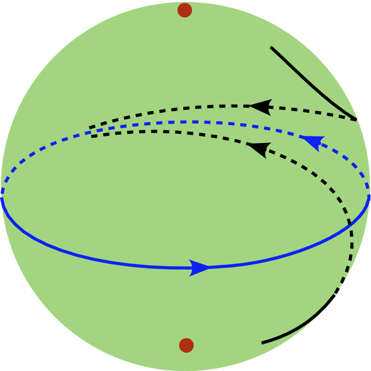
Note that the coordinate plane
$z = 0$
 is invariant. Hence, the equator of
$\mathbb S^2$
 is a limit cycle. Since the third component of the vector field F in (1.2) is negative for
$0 < z < 1$
 and positive for
$-1 < z < 0$
 , the equator of
$\mathbb S^2$
 is a stable limit cycle (see Figure 2 for an illustration).
Some orbits of the differential equation (1.2) with Q given in (3.2) on the unit invariant sphere
$\mathbb S^2$
 . The unstable foci
$(0,0,1)$
 and
$(0,0,-1)$
 are draw in red. The equator of the invariant sphere
$\mathbb S^2$
 is a stable limit cycle and is draw in blue. Two positive orbits corresponding to the initial conditions
$(1/2,0,\pm \sqrt {3}/2)$
 are drawn in black. For interpretation of the references to color in this figure legend, the reader is referred to the web version of the article.

Example 3.3 Consider
$Q: \mathbb R^3 \to \mathbb R^3$
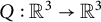 ,

a homogeneous polynomial map of degree
$3$
 in the differential equation (1.2). Note that

It follows from Theorem 1.1 that there exists a unique two-dimensional topological sphere
$S(\mu = 1) \subset \mathbb R^3 \setminus \{(0, 0, 0)\}$
 invariant by the flow of (1.2). This topological sphere
$S(1)$
 is embedded as a topological submanifold of
$\mathbb R^3$
 , and the bounded component of the complement of
$S(1)$
 contains the origin of
$\mathbb R^3$
 . Furthermore,
$S(1)$
 is globally attracting, that is, every trajectory of (1.2) with initial condition
$(x,y,z) \neq (0,0,0)$
 converges to
$S(1)$
 . By Theorem 1.2, the topological sphere
$S(1)$
 is not the unit sphere
$\mathbb S^2$
 .
Note that the planes
$x = \pm 1$
 ,
$y = \pm 1$
 , and
$z = \pm 1$
 are invariant. So, the topological sphere
$S(1)$
 is precisely the cube with vertices at the points

In addition to the six invariant planes described above, there are three more invariant planes:
$x = 0$
 ,
$y = 0$
 , and
$z = 0$
 . The 9 invariant planes determine 27 invariant straight lines; so, there are 27 equilibrium points, one of which is
$(0,0,0)$
 and the other 26 are on the invariant cube: the vertices denoted by
$p_i$
 ,
$i = 1, \ldots , 8$
 ; the midpoints of each of the 12 edges of the cube denoted by
$q_i$
 ,
$i= 1, \ldots , 12$
 ; and the centers of each of the 6 faces of the cube denoted by
$r_i$
 ,
$i = 1, \ldots , 6$
 . By a direct calculation, the equilibrium points
$p_i$
 ,
$i = 1, \ldots , 8$
 are stable nodes, the equilibrium points
$q_i$
 ,
$i = 1, \ldots , 12$
 are saddles, and the equilibrium points
$r_i$
 ,
$i = 1, \ldots , 8$
 are unstable nodes for the restriction of the differential equation (1.2) on the invariant cube (see Figure 3).
Restriction of the vector field F given in (1.2) with Q given in (3.3) to each face of the topological sphere
$S(1)$
 (cube). The nine equilibrium points are draw in red. For interpretation of the references to color in this figure legend, the reader is referred to the web version of the article.

Figure 3 Long description
The vector field is displayed on a square light green surface. Nine red circular dots represent equilibrium points. One dot is located at the exact center of the square. Four dots are located at the corners of the square, and four dots are located at the midpoints of each of the four edges. Black arrows represent the vector field F. From the central red dot, arrows flow outward in all directions toward the edges. Along the horizontal and vertical centerlines, the arrows point directly away from the center toward the edge midpoints. In the four quadrants created by these centerlines, the arrows curve symmetrically, originating from the central region and terminating or converging toward the perimeter equilibrium points. The density of the arrows is uniform across the surface, illustrating a source-like behavior from the center point.
Example 3.4 Consider the differential equation (1.2) with the homogeneous polynomial map of degree
$3$


where

As

for all
$(x, y, z) \neq (0, 0, 0)$
 , it follows from Theorem 1.1 that there exists a unique two-dimensional topological sphere
$S(\mu = 1) \subset \mathbb R^3 \setminus \{(0, 0, 0)\}$
 which is invariant by the flow of (1.2). This topological sphere
$S(1)$
 is embedded as a topological submanifold of
$\mathbb R^3$
 , and the bounded component of the complement of
$S(1)$
 contains the origin of
$\mathbb R^3$
 . Furthermore,
$S(1)$
 is globally attracting, that is, every trajectory of (1.2) through
$(x, y, z) \neq (0, 0, 0)$
 tends to
$S(1)$
 . By Theorem 1.2, the invariant topological sphere
$S(1)$
 is not the unit sphere
$\mathbb S^2$
 .
By a direct calculation, in addition to the equilibrium point at the origin, there are two equilibrium points on the topological sphere
$S(1)$


with five decimals round-off precision. The equilibrium points
$p_1$
 and
$p_2$
 are both stable foci for the restriction of the differential equation (1.2) on the invariant topological sphere
$S(1)$
 . Therefore, even without explicitly knowing the invariant topological sphere
$S(1)$
 , there exists at least one limit cycle on it (see Figure 4).
Some orbits of the differential equation (1.2) with Q given in (3.4). The stable foci
$p_1$
 and
$p_2$
 are draw in red. These two equilibrium points belong to the invariant topological sphere
$S(1)$
 . For interpretation of the references to color in this figure legend, the reader is referred to the web version of the article.

Figure 4 Long description
A phase portrait of a differential equation on a white background.
* On the left, a blue trajectory begins at a black dot at the bottom center and curves upward and to the left, forming a series of concentric, tightening loops. These loops spiral inward toward a central red dot, identified as the stable focus P sub 1.
* On the right, a black trajectory begins at a black dot at the top center and curves downward and to the right. It forms a similar series of tightening loops that spiral inward toward a second red dot, identified as the stable focus P sub 2.
* Both sets of orbits exhibit asymptotic behavior as they approach their respective equilibrium points on the invariant topological sphere S super 2 open parenthesis 1 close parenthesis.
Example 3.5 Consider the differential equation (1.2) initially in
$\mathbb R^2$
 with the homogeneous polynomial map of degree
$3$


It follows that

By Theorem 1.2, the unit sphere
$\mathbb S^1$
 is invariant by the flow of (1.2). In this case, the sphere is the unit circle. The origin
$(0,0)$
 is the unique equilibrium point of the differential equation (1.2). Thus, each orbit of the differential equation (1.2) by an initial condition different from the origin has the unit circle
$\mathbb S^1$
 as the
$\omega $
 -limit set.
Now consider the differential equation (1.2) in
$\mathbb R^4$
 defined by

that is, the differential equation (1.2) is defined in
$\mathbb R^4$
 with the homogeneous polynomial map of degree
$3$


By a direct calculation, we get

for all
$(x, y, z, w) \neq (0, 0, 0, 0)$
 . It follows from Theorem 1.1 that there exists a unique three-dimensional topological sphere
$S(\mu = 1) \subset \mathbb R^4 \setminus \{(0, 0, 0, 0)\}$
 which is invariant by the flow of (1.2). This topological sphere
$S(1)$
 is embedded as a topological submanifold of
$\mathbb R^4$
 , and the bounded component of the complement of
$S(1)$
 contains the unique equilibrium point at the origin of
$\mathbb R^4$
 . Furthermore,
$S(1)$
 is globally attracting, that is, every trajectory of (1.2) through
$(x, y, z, w) \neq (0, 0, 0, 0)$
 tends to
$S(1)$
 . It follows from Theorem 1.2 that the invariant topological sphere
$S(1)$
 is not the unit sphere
$\mathbb S^3$
 .
Consider the initial condition
$x_0 = (0, 1, 0, 1)$
 . By a direct calculation, the function

is the solution of the initial value problem defined by differential equation (1.2) and
$x_0$
 . The image of
$\gamma $
 is a periodic orbit.
Consider the torus

the Cartesian product of two circles
$\mathbb S^1 \times \mathbb S^1$
 . By the above calculations, it follows that

The construction presented in Example 3.5, where the differential equation (1.2) in
$\mathbb R^4$
 is obtained from the product of two differential equations in
$\mathbb R^2$
 with separate variables, provides a simple example of an invariant topological sphere that does not coincide with the sphere
$\mathbb S^3$
 .
In the next example, we slightly modify the differential equation (3.5) in order to obtain
$\mathbb S^3$
 as the invariant sphere.
Example 3.6 Consider the differential equation (1.2) in
$\mathbb R^4$
 defined by

that is, the differential equation (1.2) is defined in
$\mathbb R^4$
 with the homogeneous polynomial map of degree
$3$
 ,
$Q: \mathbb R^4 \to \mathbb R^4$
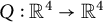 ,

where

By a direct calculation, we obtain

for all
$(x, y, z, w) \neq (0, 0, 0, 0)$
 . It follows from Theorem 1.2 that the unit sphere
$\mathbb S^3$
 is invariant by the flow of (1.2) and it is globally attracting. The bounded component of the complement of
$\mathbb S^3$
 contains the unique equilibrium point at the origin of
$\mathbb R^4$
 .
Data availability statement
No data were used for the research described in the article.
Acknowledgments
The authors thank their colleague Antonio Carlos Fernandes for the conversations regarding the subject studied here. The second author is grateful for the warm hospitality of the Universitat Autònoma de Barcelona during the development of this article.
Author contributions
All authors have collaborated equally in the preparation of this manuscript. The author ordering is alphabetical.
Competing interests
The authors declare that they have no known competing financial interests or personal relationships that could have appeared to influence the work reported in this article.