1 Introduction

The uncertainty principle is a fundamental concept asserting that no function can be simultaneously localized in both position and frequency. This principle carries profound implications throughout mathematics and physics. Recently, Dyatlov and Zahl [Reference Dyatlov and ZahlDZ] introduced the fractal uncertainty principle (FUP), which provides a quantitative limitation on how a function and its Fourier transform may both concentrate near fractal sets. Since its introduction, the FUP has become a central theme in Fourier analysis and has deep connections with other fields, including chaotic dynamics, spectral theory, and scattering theory.

The FUP has been established in a variety of one-dimensional settings through several distinct approaches: additive combinatorics [Reference Dyatlov and ZahlDZ, Reference Cladek and TaoCT], Fourier decay of fractal measures [Reference Bourgain and DyatlovBD1], dynamical techniques [Reference Dyatloy and JinDJ2, BLT], and Beurling–Malliavin theory [Reference Bourgain and DyatlovBD2, Reference CohenC2]. Higher-dimensional extensions have also been obtained; see, for instance, Han and Schlag [Reference Han and SchlagHS] and Cohen [Reference CohenC1, Reference CohenC2].

To illustrate one of its central applications, consider an open quantum system. Resonant states oscillate while allowing energy to escape to infinity. The spectral gap governs the slowest rate of decay, thereby determining the asymptotic rate of energy dissipation with significant consequences for the stability of nonlinear wave equations. Resonant states associated with the slowest decay typically concentrate near trapped sets, that is, points that remain confined because of the underlying classical dynamics. Because of the chaotic nature of such systems, these trapped sets exhibit a fractal structure. The FUP imposes a quantitative restriction on the localization of resonant states, leading directly to estimates for the spectral gap.

Two principal examples of chaotic systems illustrating this mechanism are as follows. (1) Open baker’s maps, a canonical example of a discrete chaotic dynamical system, where the trapped sets are Cantor sets. In this setting, the FUP leads directly to a spectral gap for the corresponding quantum baker’s maps [Reference Dyatlov and JinDJ1, Reference Eswarathasan and HanEH]. (2) The geodesic flow on convex cocompact hyperbolic surfaces, a prominent example of a continuous chaotic dynamical system, where the trapped sets correspond to Schottky limit sets. The FUP established for these Schottky limit sets has contributed directly to recent breakthroughs on the spectral gap for the Laplacian in this geometry [Reference Bourgain and DyatlovBD1, Reference Bourgain and DyatlovBD2, Reference Dyatlov and ZahlDZ]. For a comprehensive overview of the FUP and its applications to open systems, as well as to eigenfunction estimates in closed systems, we refer the reader to Dyatlov’s survey article [Reference DyatlovDy].

We now state the formal framework of the FUP. Let $0<h\le 1$ denote the semiclassical parameter and define the semiclassical Fourier transform

$$ \begin{align*} \mathcal{F}_hu(\xi)=\frac{1}{\sqrt{2\pi h}}\int_{\mathbb{R}}e^{-({ix\cdot \xi}/{h})}u(x)\,dx\quad\text{for }u\in C_0^\infty(\mathbb{R}). \end{align*} $$

For $h=1$ , this coincides with the standard Fourier transform $\mathcal {F}:=\mathcal {F}_1$ . The FUP concerns estimates for the operator norm

(1-1)

where the h-dependent sets $X=X(h)$ and $Y=Y(h)\subset \mathbb {R}$ have fractal-type geometry characterized by $\delta $ -regularity, following Dyatlov [Reference DyatlovDy, Definition 2.2].

Definition 1.1 ( $\delta $ -regular sets).

Let $0\le \delta \le 1$ , $R\ge 1$ , and $0\le \alpha _{\mathrm {min}}\le \alpha _{\mathrm {max}}\le \infty $ . A nonempty closed set $X\subset \mathbb {R}$ is called $\delta $ -regular with constant R on scales $\alpha _{\mathrm {min}}$ to $\alpha _{\mathrm {max}}$ if there exists a locally finite measure $\nu _X$ supported on X such that, for every interval I centered at a point of X with $\alpha _{\mathrm {min}}\le |I|\le \alpha _{\mathrm {max}}$ ,

$$ \begin{align*}R^{-1}|I|^\delta\le\nu_X(I)\le R|I|^\delta.\end{align*} $$

Here, $|E|$ denotes the Lebesgue measure of a measurable set $E\subset \mathbb {R}$ .

Since $\mathcal {F}_h$ is unitary on $L^2(\mathbb {R})$ , we always have (1-1) $=O(1)$ . We say that X and Y satisfy the FUP with exponent $\beta \ge 0$ if (1-1) $=O(h^\beta )$ as $h\to 0$ . The main goal in studying the FUP for $\delta $ -regular sets is to establish the existence of an exponent $\beta>0$ and to determine the sharp exponent for which the FUP holds. The sharp exponent, denoted by $\beta ^s(X,Y)$ , is the largest $\beta $ such that (1-1) $=O(h^\beta )$ holds for all $0<h<h_0$ with some $h_0>0$ . It typically depends on the parameters $\delta $ and R in Definition 1.1 associated with the sets X and Y.

First, if X and Y are $\delta $ -regular on scales h to $1$ with $\delta \in [0,1]$ , then the FUP (1-1) holds with exponent

(1-2) $$ \begin{align} \beta_{\mathrm{Vol}}=\max\{\tfrac{1}{2}-\delta,0\}. \end{align} $$

This quantity (1-2) is sometimes referred to as ‘the volume bound’, as it depends only on the volumes of X and Y, namely $|X|,|Y|\le Ch^{1-\delta }$ ; see Bourgain and Dyatlov [Reference Bourgain and DyatlovBD2, Lemma 2.9].

Improvements over the volume bound (1-2) have been obtained in various settings; see, for example [Reference Dyatloy and JinDJ2, Reference Jin and ZhangJZ]. The sets considered in these works are deterministic and the improvement in the exponent is generally small (and either implicitly or explicitly dependent on $\delta $ and R in Definition 1.1). In particular, the following theorem includes explicit estimates on such improvements, which are exponentially small when $0<\delta \le \frac 12$ [Reference Dyatloy and JinDJ2, Theorem 1] and superexponentially small when $\frac 12<\delta <1$ [Reference Jin and ZhangJZ, Theorem 1.2].

Theorem 1.2. Let $0<\delta <1$ and $R\ge 1$ . Suppose that $X,Y$ are $\delta $ -regular with constant R on scales h to $1$ . Then, the FUP (1-1) holds with an exponent $\beta $ such that

$$ \begin{align*} \beta-\beta_{\mathrm{Vol}}\ge\begin{cases} (5R)^{-({40}/{\delta(1-\delta)})} & \text{if }\ 0<\delta\le\tfrac12,\\ \exp[-\exp(C(R\delta^{-1}(1-\delta)^{-1})^{C(1-\delta)^{-2}})] & \text{if }\ \tfrac12<\delta<1. \end{cases}\end{align*} $$

Here, $C>0$ is an absolute constant.

In an ongoing project, we investigate the FUP (1-1) when the sets $X,Y$ are constructed via certain random procedures, and in these random settings, we aim to prove the FUP with more favorable exponents than those in Theorem 1.2 for the deterministic cases. Eswarathasan and the first-named author [Reference Eswarathasan and HanEH] considered the FUP for the random Cantor sets in the discrete setting. That is, let $M,A\in \mathbb {N}$ such that $M\ge 3$ and $A=M^\delta $ with $0<\delta <1$ . Then, the alphabets of cardinality A from the digits $\{0,\ldots ,M-1\}$ form a probability space

$$ \begin{align*} \mathbb{A}(M,A)=\{\mathcal{A}\subset\{0,\ldots,M-1\}:\mathrm{Card}(\mathcal{A})=A\}, \end{align*} $$

which is equipped with the uniform counting measure $\mu _1$ . Here, $\mathrm {Card}(\mathcal {A})$ is the cardinality of $\mathcal {A}$ .

In [Reference Eswarathasan and HanEH], an alphabet is chosen at random from $\mathbb {A}(M,A)$ ; then the discrete Cantor sets are constructed using this alphabet (in each iteration step). Let $\delta \in (0,\frac 23)$ . 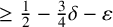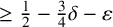We proved that, with overwhelming probability (that is, except on a subset of $\mathbb {A}(M,A)$ with exponentially small measure depending on $M,\varepsilon $ ), the Cantor sets with random alphabets satisfy the FUP with an exponent $\beta \ge \frac 12-\frac 34\delta -\varepsilon $ . It is a significant improvement over the volume bound (1-2) for this random ensemble.

In this paper, we consider the FUP for random Cantor sets in the continuous setting of $\mathbb {R}$ . We use a different random procedure to that in [Reference Eswarathasan and HanEH] for the construction. See Section 1.1 for the different random ensembles of Cantor sets, as well as the comparison of approaches and results between the discrete and continuous settings.

Each Cantor set in $\mathbb {R}$ can be built via an iteration process. Let $\mathbb {A}(M,A)$ be as above. Inductively define

$$ \begin{align*}B_1=\frac1M\mathcal{A}\quad\text{where }\mathcal{A}\in\mathbb{A}(M,A),\end{align*} $$

and for $j\ge 2$ ,

$$ \begin{align*} B_j=\bigcup_{b\in B_{j-1}}\bigg\{b+\frac{a}{M^j}:a\in\mathcal{A}(b)\bigg\}, \end{align*} $$

where $\mathcal {A}(b)\in \mathbb {A}(M,A)$ with $b\in B_{j-1}$ are independent and identically distributed random variables. In particular, $\mathrm {Card}(B_j)=A^j$ for all $j\in \mathbb {N}$ .

Write

(1-3) $$ \begin{align} \mathcal{C}_j=\bigcup_{b\in B_j}\bigg[b,b+\frac{1}{M^j}\bigg]\quad\text{and}\quad\mathcal{C}=\bigcap_{j=1}^\infty\mathcal{C}_j\subset[0,1]. \end{align} $$

Hence, $\mathcal {C}_j$ is a union of $A^j$ closed intervals, each of which has Lebesgue volume of $M^{-j}$ . Define also the Borel measure $\nu _j$ whose density function is given by

Finally, the weak limit $\nu $ of $\nu _j$ as $j\to \infty $ defines the Cantor measure which is supported on $\mathcal {C}$ .

We next set up the appropriate probability space for the random Cantor set $\mathcal {C}$ and the random Cantor measure $\nu $ . In the first iteration, the probability space is given by $\mathbb {A}(M,A)$ ; in the j th iteration for $j\ge 2$ , since $\mathrm {Card}(B_{j-1})=A^{j-1}$ , the probability space is given by $\mathbb {A}(M,A)^{A^{j-1}}$ equipped with the uniform counting measure $\mu _j$ . Write

(1-4) $$ \begin{align} \mathbb{A}^\infty:=\prod_{j=1}^\infty\mathbb{A}(M,A)^{A^{j-1}}\quad \text{equipped with the probability measure }\mu^\infty:=\prod_{j=1}^\infty\mu_j. \end{align} $$

Then, $\mathcal {C}$ is a random Cantor set and $\nu $ is a random Cantor measure in $\mathbb {R}$ with respect to the probability space $\mathbb {A}^\infty $ .

It is obvious that each Cantor set $\mathcal {C}$ constructed in this way has Hausdorff dimension

$$ \begin{align*}\delta=\frac{\log A}{\log M}\in(0,1).\end{align*} $$

Moreover, each Cantor set $\mathcal {C}$ is $\delta $ -regular with constant $R=2$ on scales $0$ to $1$ , for which one can simply choose the Cantor measure $\nu $ in Definition 1.1; see [Reference DyatlovDy, Example 2.6] for the example of the middle-third Cantor set (that is, $M=3$ and $\mathcal {A}=\{0,2\}$ ).

Consider the h-neighborhoods $\mathcal {C}(h)$ of $\mathcal {C}$ . Then, $\mathcal {C}(h)$ is $\delta $ -regular with constant $R=8$ on scales h to $1$ ; see [Reference Bourgain and DyatlovBD2, Lemma 2.3]. Therefore, for each Cantor set $\mathcal {C}$ , the FUP (1-1) holds for $X=Y=\mathcal {C}(h)$ with an exponent $\beta $ explicitly given in Theorem 1.2.

However, in the case when $0<\delta <\frac 23$ , we prove that, with overwhelming probability (that is, except on a subset of $\mathbb {A}^\infty $ with exponentially small measure), the FUP holds for the random Cantor sets with much better exponents than those in Theorem 1.2.

Theorem 1.4 (FUP for random Cantor sets).

Let $0<\delta <\frac 23$ . Suppose that $M,A\in \mathbb {N}$ such that $M\ge 2^{(4/\delta )}$ and $A=M^\delta $ . Then, for $0<\varepsilon <(\delta /2)$ , there exists $\mathbb {G}\subset \mathbb {A}^\infty $ with

$$ \begin{align*} \mu^\infty(\mathbb{A}^\infty\setminus\mathbb{G})\le C_1e^{-({M^\varepsilon})/{C}} \end{align*} $$

such that each Cantor set $\mathcal {C}$ from $\mathbb {G}$ satisfies that

Here, $C>0$ is an absolute constant and $C_1=C_1(\varepsilon )>0$ depends on $\varepsilon $ .

We also prove an FUP for the random Cantor measures $\nu $ .

Theorem 1.5 (FUP for random Cantor measures).

Under the same conditions as Theorem 1.4, the corresponding random Cantor measure $\nu $ satisfies that

$$ \begin{align*} \bigg\|\!\int_{\mathbb{R}}e^{-({ix\cdot \xi})/{h}}u(x)\,d\nu(x)\bigg\|_{L^2_\nu(\mathbb{R})} \le Ch^{(\delta/4)-\varepsilon}\|u\|_{L^2_\nu(\mathbb{R})}\quad\text{for all }u\in L^2_\nu(\mathbb{R}) \text{ and } 0<h<M^{-8}. \end{align*} $$

The proofs of the FUP in Theorems 1.4 and 1.5 are based on the following Fourier decay estimate of the random Cantor measures.

Theorem 1.6 (Fourier decay of random Cantor measures).

Let $0<\delta <1$ . Suppose that $M,A\in \mathbb {N}$ such that $M\ge 2^{(4/\delta )}$ and $A=M^\delta $ . Then, for $0<\varepsilon <\min \{(\delta /2),\frac 13\}$ , there exists $\mathbb {G}\subset \mathbb {A}^\infty $ with

$$ \begin{align*} \mu^\infty(\mathbb{A}^\infty\setminus\mathbb{G})\le C_1e^{-({M^\varepsilon}/{C})} \end{align*} $$

such that each Cantor measure $\nu $ from $\mathbb {G}$ satisfies that

(1-5) $$ \begin{align} |\mathcal{F}\nu(\xi)|\le C|\xi|^{-({\delta-\varepsilon}/{2})}\quad\text{for all }|\xi|\ge M^4. \end{align} $$

Here, $C>0$ is an absolute constant and $C_1=C_1(\varepsilon )>0$ depends on $\varepsilon $ .

1.1 Random ensembles in the discrete setting and the continuous setting

Continue with our notation of $\mathbb {A}(M,A)$ with $M,A\in \mathbb {N}$ and $A=M^\delta $ , $0<\delta <1$ . We discuss the FUP for different ensembles of Cantor sets. The boundary points of the Cantor set in the continuous setting of $\mathbb {R}$ at each iteration $j\in \mathbb {N}$ naturally define the Cantor set in the discrete setting of

$$ \begin{align*}\mathbb{Z}_N:=\frac1N\mathbb{Z}/N\mathbb{Z}\quad\text{with }N=M^j.\end{align*} $$

This connection allows us to compare the approaches and results on the FUP in the discrete setting and in the continuous setting. (We remark that for direct comparison between the two settings, the discrete set $\mathbb {Z}_N$ here differs to that in [Reference Dyatlov and JinDJ1, Reference Eswarathasan and HanEH] by a scaling factor of N.)

Ensemble I. Let $\mathcal {A}\in \mathbb {A}(M,A)$ be randomly chosen. For $j\in \mathbb {N}$ , define the discrete Cantor set of order j as

$$ \begin{align*} B_j=\bigg\{\!\sum_{l=1}^j\frac{a_l}{M^l}:a_l\in\mathcal{A}\text{ for }l=1,\ldots,j\bigg\} \end{align*} $$

for which the probability space is $\mathbb {A}(M,A)$ .

Ensemble II. For $j\in \mathbb {N}$ , let $\mathcal {A}_k\in \mathbb {A}(M,A)$ for $l=1,\ldots ,j$ be independent and identically distributed random variables. Define the discrete Cantor set of order j as

$$ \begin{align*} B_j=\bigg\{\!\sum_{l=1}^j\frac{a_l}{M^l}:a_l\in\mathcal{A}_l\text{ for }l=1,\ldots,j\bigg\} \end{align*} $$

for which the probability space is $\prod _{l=1}^j\mathbb {A}(M,A)$ .

Ensemble III. Let $B_1=(1/M)\mathcal {A}$ with $\mathcal {A}\in \mathbb {A}(M,A)$ . For $j\ge 2$ , let $\mathcal {A}(b)\in \mathbb {A}(M,A)$ for $b\in B_{j-1}$ be independent and identically distributed random variables, and define the discrete Cantor set of order j as

$$ \begin{align*} B_j=\bigcup_{b\in B_{j-1}}\bigg\{b+\dfrac{a}{M^j}:a\in\mathcal{A}(b)\bigg\} \end{align*} $$

for which the probability space is $\prod _{k=1}^j\mathbb {A}(M,A)^{A^{k-1}}$ .

Figure 1

The initial three iterations and the alphabet used for a Cantor set in Ensemble I. (The intervals colored red are removed in the iteration process.)

Figure 2

The initial three iterations and the alphabets used for a Cantor set in Ensemble II.

Figure 3

The initial three iterations and the alphabets used for a Cantor set in Ensemble III.

Figure 3 Long description

A multi-panel diagram showing three iterations of a Cantor set.

Row 1: A horizontal line divided into three segments labeled 0, 1, and 2. Segments 0 and 1 are black, while segment 2 is red. To the right is the set notation {0, 1}.

Row 2: The line is further subdivided into six segments. From left to right, the labels are 0 (black), 1 (red), 2 (black), 0 (black), 1 (black), and 2 (red). To the right are the sets {0, 2}, {1, 2}.

Row 3: The line consists of several smaller segments. The first group has labels 0 (red), 1 (black), 2 (black). After a gap, a longer sequence of segments is labeled 0 (red), 1 (black), 2 (black), 0 (black), 1 (red), 2 (black), 0 (black), 1 (black), 2 (red). To the right are the sets {1, 2}, {1, 2}, {0, 2}, {0, 1}.

In each of these ensembles, the Cantor sets $\mathcal {C}$ in $\mathbb {R}$ are defined by (1-3). Figures 1–3 demonstrate (the initial iterations of) examples of the Cantor sets with $M=3$ and $A=2$ .

Remark 1.8 (The FUP for Cantor sets in the discrete setting of $\mathbb {Z}_N$ ).

Let $\mathcal {F}_N$ be the discrete Fourier transform that is unitary on $l^2(\mathbb {Z}_N)$ . For each $j\in \mathbb {N}$ , the discrete Cantor set $B_j\in \mathbb {Z}_N$ . The FUP for Cantor sets in the discrete setting is concerned with the estimate of the form

(1-6)

where $N^{-1}=M^{-j}\to 0$ plays the role of the semiclassical parameter.

For the deterministic Cantor sets in Ensemble I, Dyatlov and Jin [Reference Dyatlov and JinDJ1] introduced an FUP theory and proved the FUP (1-6) with exponent $\beta =\beta (M,\mathcal {A})>\beta _{\mathrm {Vol}}$ for all $M,\mathcal {A}$ . They also extensively studied the sharp exponent $\beta _s(M,\mathcal {A})$ in the FUP for different $M,\mathcal {A}$ . On one hand, they found examples of $M,\mathcal {A}$ for which the FUP holds with the exponent ${1-\delta }/{2}$ , which is the best possible one. On the other hand, they also found examples of $M,\mathcal {A}$ for which the sharp exponent $\beta _s(M,\mathcal {A})=\beta _{\mathrm {Vol}}+o_M(1)$ ; see [Reference HuH] and [Reference KangabireK] for more recent constructions of Cantor sets for such examples.

For the random Cantor sets in Ensemble I, Eswarathasan and Han [Reference Eswarathasan and HanEH] introduced a probabilistic approach to the FUP and proved that for $0<\delta <\frac 23$ , $\beta _s(M,\mathcal {A})\ge \frac 12-\frac 34 \delta -\varepsilon $ with overwhelming probability. The proof is similar to that used in this paper; that is, it is based on establishing a Fourier decay estimate of the corresponding discrete Cantor measure $\tilde \nu _j=\sum _{b\in B_j}\delta _b$ . However, the proof is simplified because of the submultiplicativity property in the discrete setting: if $j=j_1+j_2$ , then

where $N=N_1N_2$ with $N_1=M^{j_1}$ and $N_2=M^{j_2}$ . Hence, the estimate of the FUP at the initial iteration $j=1$ implies one for all iterations $j\in \mathbb {N}$ . Indeed, the Fourier transform of the discrete Cantor measure at the first iteration,

$$ \begin{align*} \mathcal{F}\tilde\nu_1(m)\quad\text{where }\tilde\mu_1=\sum_{b\in B_1}\delta_b=\sum_{a\in\mathcal{A}}\delta_{a/M}, \end{align*} $$

has decay for $m\in \mathbb {Z}_M\setminus \{0\}$ for randomly chosen $\mathcal {A}\in \mathbb {A}(M,A)$ , which is sufficient to imply the FUP in the discrete setting.

For the deterministic Cantor sets in Ensembles II and III, one can prove an FUP with exponents in Theorem 1.2, following an approach of Dyatlov and Jin [Reference Dyatloy and JinDJ2] to reduce the FUP for the discrete Fourier transform $\mathcal {F}_N$ to one for $\mathcal {F}_h$ with respect to the discrete measures $\tilde \nu _j$ . Moreover, Dyatlov and Jin [Reference Dyatlov and JinDJ1] still supply examples of Cantor sets for which the FUP holds with the best possible exponent (by simply choosing the same alphabet at each iteration).

However, much less is known for the random Cantor sets in Ensembles II and III than Ensemble I. In particular, the submultiplicativity property is not necessarily true, since different alphabets can be used in different iterations. Thus, one has to consider higher iterations when proving the FUP via the probabilistic approach. This is open.

Remark 1.9 (The FUP for Cantor sets in the continuous setting of $\mathbb {R}$ ).

All Cantor sets $\mathcal {C}$ in each ensemble above are $\delta $ -regular with an absolute constant R on scales $0$ to $1$ in Definition 1.1. Their h-neighborhoods $\mathcal {C}(h)$ are $\delta $ -regular on scales h to $1$ . As a consequence, the h-neighborhoods $\mathcal {C}(h)$ satisfy the FUP in Theorem 1.2.

Our main results in Theorems 1.4 and 1.5 are concerned with the random Cantor sets in Ensemble III, stating that if $0<\delta <\frac 23$ , then the sharp constant $\beta _s\ge \frac 12-\frac 34\delta -\varepsilon $ in the FUP with overwhelming probability.

However, for the random Cantor sets in Ensembles I and II, much less is known. In particular, the Cantor measures in these ensembles do not necessarily have Fourier decay; that is, the Fourier dimension of some Cantor sets can be zero; see again [Reference MattilaM, Ch. 12]. The probabilistic approach to the FUP in these ensembles is open.

Moreover, for the deterministic case in all the above-mentioned ensembles, no examples of Cantor sets are known to satisfy the FUP with the best possible exponent ${1-\delta }/{2}$ in the continuous setting of $\mathbb {R}$ to the authors’ knowledge.