Nomenclature
- x
-
covariates
- y
-
response variable
- n
-
sample size
- S
-
number of quantiles
- d
-
similarity between target and sources
- h
-
bandwidth
- K
-
number of sources
- G
-
composite quantile loss function
- g
-
the subgradient of the loss function
- H
-
overall Hessian matrix
Greek symbol
-
 $ \tau $
-
composite quantile level
-
$ \epsilon $
-
random error
-
$ \beta $
-
regression coefficient
-
$ \lambda $
-
penalty term
-
$ \delta $
-
bias term
-
$ \mathcal{A}\mathcal{}$
-
informative set


1.0 Introduction
With the continuous growth of civil aviation passenger traffic, aviation management has become a global concern. A core component of modern aviation management is flight safety monitoring, which relies on analysing large-scale data recorded by the quick access recorder (QAR). This process not only involves real-time recording and anomaly identification of flight status, but also is an important basis for aviation safety management, accident prevention and policy optimisation. QAR data records aircraft attitude parameters and engine-related data at different stages, which provides effective data support for evaluating pilot operation level, improving aircraft performance and optimising flight technology. Currently, researchers are committed to analysing and predicting flight risks by building data-driven models to reduce the occurrence of aviation accidents. QAR data has its own unique analysis challenges. The data are high-dimensional, with complex and non-normally distributed relationships among variables. It is more critical that there are significant differences in data distribution across aircraft types and airlines. These differences lead to the problem that when constructing traditional prediction models based on the single source data, new aircraft types and some routes encounter a smaller sample size, and the generalisation ability and prediction accuracy do not meet the demand.
In order to study the relationship between landing distance and flight parameters, Wang et al. [Reference Wang, Wu and Sun1] established logistic regression and linear regression models, respectively. The traditional mean regression can only capture the central trend of the distribution, while the flight safety problem often involves the extreme situations, which generally exist at the tail of the conditional distribution of the response variable. Therefore, Chen et al. [Reference Chen, Liu and Mao2] employed quantile regression to identify the key factors affecting the maximum vertical acceleration during the landing phase and used the dimension reduction method to verify the results. Finally, the form of the action of key factors on hard landing was systematically expounded. More recently, Zhao J et al. [Reference Zhao, Rong and Dang3] proposed the use of generative adversarial networks to fill missing values in QAR data and achieved a significant improvement in data quality by introducing a self-attention mechanism. However, the problem of insufficient sample size of new aircraft models has not been solved. We consider transfer learning to transfer from existing tasks, so as to achieve better performance on limited datasets [Reference Tibshirani4, Reference Fan and Li5].
A central issue in transfer learning is how to effectively transfer the information from the sources to the target. Using only target data will ignore the information from the sources that may be useful. If all sources are used, it may ignore the potential heterogeneity between the sources and the target, resulting in ‘negative transfer’. The heterogeneity between domains is mainly manifested as the following three aspects. (1) Data distribution differences: the distribution of covariate
 $ f({\boldsymbol{x}}_{i})$
may be different, which is called covariate shift in some related literature. (2) Model differences: there may also be differences in the regression coefficients of the conditional distribution
 $ f({y}_{i}\,|\,{\boldsymbol{x}}_{i})$
. (3) Error distribution differences: the error distribution of different models may also be significantly different.
The current transfer learning framework mainly solves the first two heterogeneous problems [Reference Li6]. Li et al. [Reference Li, Cai and Li7] considered the complex situation of multiple sources, proposed a two-step transfer learning algorithm under the high-dimensional linear model, and further discussed how to detect the informative set when the informative set is unknown. Tian and Feng [Reference Tian and Feng8] extended the two-step transfer learning algorithm to generalised linear model and proposed a more simple informative set detection method, which made multi-source transfer learning more efficient and convenient. Chen et al. [Reference Chen, Liu and Mao2] studied the high-dimensional linear regression model with heavy-tailed noise and established a new relationship between quantile regression and linear regression by transforming the response variables. Jin et al. [Reference Jin, Yan and Aseltine9] developed a transfer learning method for high-dimensional quantile regression, which achieves smaller errors based on sample size, signal-to-noise ratio, etc.
In the practical application of QAR data, we may not be able to determine a specific quantile point. Through residual analysis, we can find that the data does not obey the normal distribution and has heteroscedasticity, and the variables are scattered near the adjacent quantile points. This situation will be unstable due to the quantile point disturbance. Quantile regression shows its superiority in dealing with data heterogeneity and heavy-tailed error [Reference Fan, Li and Wang10–Reference Koenker and Bassett13]. Zou and Yuan [Reference Zou and Yuan14] proposed the composite quantile regression (CQR) model, which considers multiple quantile points and captures the distribution information of different quantile points of the data. The theoretical results show that this not only improves the performance of the model, but also enhances the adaptability to complex data distribution. In view of the above challenges, we propose a transfer learning based on the composite quantile regression model, which uses the source data to assist the target modeling and synthesises multiple quantile information, so as to make the estimation more robust.
Compared with the existing work under QAR data [Reference Qiao, He and Zhou15, Reference Li and Song16], the composite quantile regression model based on transfer learning proposed in this paper has several advantages. (1) A transfer learning framework for hard landing prediction of QAR data is constructed. The composite quantile loss is transformed into a linear form by Newton-Raphson iteration, so that the transfer learning can realise the composite quantile regression with non-differentiable loss. (2) This paper considers the information of multiple quantile points at the same time, and the model is more robust when the quantile points are unknown. (3) When some routes encounter a small amount of data, other source information can be introduced. The application on the QAR dataset shows that the algorithm significantly improves the performance of the model.
The rest of this article is organised as follows. In Section 2, the construction of the composite quantile regression model in transfer learning is introduced. In Section 3, the pseudo response is first constructed based on the Newton-Raphson iteration, and the transfer learning algorithm based on the composite quantile regression model is described. When the informative set is unknown, a cross-validation algorithm is proposed to detect the informative set. Section 4 presents the theoretical results of the proposed method. Section 5 provides numerical simulation results to verify the performance of the proposed algorithm. Section 6 shows the application of the algorithm in the aircraft hard landing problem. Finally, Section 7 summarises the full text and discusses the possible direction of the future work. The proofs of theorem and numerical analysis discussions are listed in the Appendix.
2.0 Transfer learning settings of composite quantile regression
2.1 Composite quantile regression model
This paper mainly studies the problem of data insufficiency and quantile perturbation in QAR data. Consider a dataset consisting of
 $ n$
independent observations
 $ \{{y}_{i},{\boldsymbol{x}}_{i}{\}}_{i=1}^{n}$
, where the response variable
 $ {y}_{i}$
and the covariate vector
 $ {\boldsymbol{x}}_{i}=({x}_{i1},\dots ,{x}_{ip}{)}^{\rm{T}}$
are collected independently from the random variables
 $ y$
and
 $ \boldsymbol{x}=({x}_{1},\dots ,{x}_{p}{)}^{\rm{T}}$
. Consider the following quantile regression model
 \begin{align} {y_i} = {{\boldsymbol{x}}_{\boldsymbol{i}}}^T{\boldsymbol{\beta}} + {\varepsilon _i},P({\varepsilon _i} \le 0|{{\boldsymbol{x}}_{\boldsymbol{i}}}) = \tau ,i = 1,2, \ldots ,n,\end{align}
where
 ${\boldsymbol{\beta}} $
is the true regression coefficient at the quantile level
 $ \tau $
, and
 $ \epsilon $
is a random error with a density function
 $ f(\!\cdot\!)$
. The covariate
 $ \boldsymbol{x}$
is independent of noise
 $ \epsilon $
. The quantile loss of the fixed quantile point is defined as
 $ {\rho }_{\tau }(u)=u[\tau \cdot {I}_{(u\ge 0)}-(1-\tau )\cdot {I}_{(u\le 0)}]$
, where
 $ I(\!\cdot\!)$
is an indicator function. Given the observed data
 $ ({\boldsymbol{x}}_{i},{y}_{i}{)}_{i=1}^{n}$
, the quantile regression estimator is obtained by solving
 \begin{align}{\hat{{\boldsymbol{\beta}}}^{QR}} = \mathop {{\rm{arg\,min}}}\limits_{\boldsymbol{\beta} \in {\mathbb {R}} {^p}} {1 \over n}\mathop \sum \limits_{i = 1}^n {\rho _\tau }\!\left( {{y_i} - {\boldsymbol{x}}_i^T{\boldsymbol{\beta}} } \right)\!.\end{align}
In practical applications, a specific quantile level may not be predetermined, and the estimation may suffer from instability due to perturbations in the quantile level. Therefore, composite quantile regression, as an extension of quantile regression, can consider the information of multiple quantile points at the same time. Suppose that there are
 $ S$
quantiles satisfying
 $ 0\le {\tau }_{1}\le {\tau }_{2}\le \dots \le {\tau }_{S}\le 1$
, the parameter estimation of composite quantile regression is the solution of the following optimisation problem
 \begin{align}{\hat{{\boldsymbol{\beta}}}^{CQR}} = \mathop {{\rm{arg\,min}}}\limits_{{\boldsymbol{\beta}} \in {{\mathbb{R}}^p}} {1 \over {nS}}\mathop \sum \limits_{s = 1}^S \mathop \sum \limits_{i = 1}^n {\rho _{{\tau _s}}}\!\left( {{y_i} - {\boldsymbol{x}}_i^T {\boldsymbol{\beta}} } \right)\!.\end{align}
2.2 Multi-source transfer learning setting
This paper extends the CQR framework to a transfer learning setting with multiple sources. It is assumed that the target dataset of the study is expressed as
 $ ({\boldsymbol{X}}^{(0)},{\boldsymbol{y}}^{(0)})\in {\mathbb{R}}^{{n}_{0}\times p}\times {\mathbb{R}}^{{n}_{0}}$
, where
 $ {n}_{0}$
is the sample size of the target dataset. There are
 $ K$
source datasets, where the
 $ k$
th source data is represented as
 $ ({\boldsymbol{X}}^{(k)},{\boldsymbol{y}}^{(k)})\in {\mathbb{R}}^{{n}_{k}\times p}\times {\mathbb{R}}^{{n}_{k}}$
, where
 $ {n}_{k}$
is the sample size of the
 $ k$
th source dataset. The parameters of the composite quantile regression model established on the
 $ k$
th dataset are denoted as
 $ {{\boldsymbol{\beta}} }^{(k)}$
,
 $ k=\rm{0,1},\dots ,K$
.
As shown in Fig. 1, the core principle of transfer learning is that if the
 $ k$
th source model has a certain degree of similarity to the target model, the information of the
 $ k$
th source dataset can be appropriately transferred and utilised. The sparsity of the difference between
 $ {{\boldsymbol{\beta}} }^{(0)}$
and
 $ {{\boldsymbol{\beta}} }^{(k)}$
is defined as the criterion for measuring the difference of the model, i.e.
 $ \| {{\boldsymbol{\delta}} }^{(k)}{\| }_{1}=\| {{\boldsymbol{\beta}} }^{(0)}-{{\boldsymbol{\beta}} }^{(k)}{\| }_{1}$
. If the similarity satisfies
 $ \| {{\boldsymbol{\delta}} }^{(k)}{\| }_{1}\le d$
, it is considered that the
 $ k$
th source is a transferable source, where
 $ d$
is a non-negative value to be specified. The informative set is a set of transferable source ordinal numbers, defined as
 $ \mathcal{A}=\left\{1\le k\le K\:\;\| {{\boldsymbol{\delta}} }^{(k)}{\| }_{1}\le d\right\}$
. It is necessary to adjust the similarity according to different needs. Excessive selection of
 $ d$
value may lead to negative transfer, that is the source information will damage the generalisation performance of the target model. If the value of
 $ d$
is too small, some potential source information may be lost. Therefore, it is necessary to select the appropriate similarity by regularisation path analysis or cross-validation.
Transfer learning graphical abstract.

3.0 Parameter estimation based on transfer learning
This section will introduce the main content of the algorithm. Firstly, the relationship between composite quantile regression and linear regression is established in the context of transfer learning, and then it is integrated into the two-step transfer learning process. Since the informative set of the target task is often unknown in practical applications, this section presents an informative set detection algorithm based on sample splitting.
3.1 Construct pseudo responses
Consider the following composite regression optimisation problem
 \begin{align} \boldsymbol {\beta}^{*} = \underset{\boldsymbol {\beta} \in \mathbb{R}^{p}}{\arg\min} E(G(\boldsymbol {\beta};\; \boldsymbol{X}, \boldsymbol{Y})),\end{align}
where the composite quantile loss is
 $ G({\boldsymbol{\beta}} ;\;\boldsymbol{X},\boldsymbol{Y})={\sum }_{s=1}^{S} {\rho }_{{\tau }_{s}}(\boldsymbol{y}-{\boldsymbol{x}}^{T}{\boldsymbol{\beta}} )$
. The Newton-Raphson iterative algorithm is based on the local quadratic approximation principle of the target function, and the roots of the equation are solved iteratively. The iterative formula of the estimation equation is as follows
 \begin{align} {\boldsymbol {\beta}}_1=\boldsymbol {\beta}_0-H(\boldsymbol {\beta}_0)^{-1}E[g(\boldsymbol {\beta}_0;\; \boldsymbol{X}, \boldsymbol{Y})],\end{align}
where
 $ \boldsymbol{\beta }_{0}$
is the initial value,
 $ g({\boldsymbol{\beta}} ;\;\boldsymbol{X},\boldsymbol{Y})$
is the subgradient of the loss function
 $ G({\boldsymbol{\beta}} ;\;\boldsymbol{X},\boldsymbol{Y})$
and
 $ H({\boldsymbol{\beta}} ):=\frac{\partial E(g({\boldsymbol{\beta}} ;\;\boldsymbol{X},\boldsymbol{Y}))}{\partial {\boldsymbol{\beta}} }$
is the overall Hessian matrix. The corresponding subgradient is given by
 $ g({\boldsymbol{\beta}} ;\;\boldsymbol{X},\boldsymbol{Y})={\sum }_{s=1}^{S} \boldsymbol{X}[I(\boldsymbol{Y}-{\boldsymbol{X}}^{T}{\boldsymbol{\beta}} \le 0)-{\tau }_{s}]$
, and the Hessian matrix is
 $ H({\boldsymbol{\beta}} )={\sum }_{s=1}^{S} E(\boldsymbol{X}{\boldsymbol{X}}^{T}f({\boldsymbol{X}}^{T}({\boldsymbol{\beta}} -{{\boldsymbol{\beta}} }^{\rm{*}})))$
,where
 $ f(\!\cdot\!)$
is the density function of the noise
 $ \epsilon $
. When the initial estimator
 $ {{\boldsymbol{\beta}} }_{0}$
is close enough to the true parameter
 $ {{\boldsymbol{\beta}} }^{\rm{*}}$
,
 $ H({{\boldsymbol{\beta}} }_{0})$
is close to
 $ H({{\boldsymbol{\beta}} }^{\rm{*}})=S\boldsymbol {\Sigma }f(0)$
, where
 $ \boldsymbol {\Sigma }=E(\boldsymbol{X}{\boldsymbol{X}}^{T})$
is the overall covariance matrix. Substituting
 $ H({{\boldsymbol{\beta}} }^{\rm{*}})$
into (5) yields
 \begin{align} {\boldsymbol {\beta}}_1=\boldsymbol {\beta}_0-H(\boldsymbol {\beta}^*)^{-1}E[g(\boldsymbol {\beta}_0;\; \boldsymbol{X}, \boldsymbol{Y})].\end{align}
The first-order Taylor expansion of
 $ E(g({{\boldsymbol{\beta}} }_{0};\;\boldsymbol{X},\boldsymbol{Y}))$
at point
 $ {{\boldsymbol{\beta}} }^{\rm{*}}$
is
 \begin{align} E(g(\boldsymbol {\beta}_0;\; \boldsymbol{X}, \boldsymbol{Y}))=H(\boldsymbol {\beta}^*)(\boldsymbol {\beta}_0-\boldsymbol {\beta}^*)+O\big(\|\boldsymbol {\beta}_0 - \boldsymbol {\beta}^*\|_2^2\big).\end{align}
Substituting this approximation into (6) yields
 \begin{align} {\| {{{\boldsymbol {\beta }}_{\boldsymbol {1}}} - {{\boldsymbol {\beta }}^*}} \|_2} & = {\| {{{\boldsymbol {\beta }}_{\boldsymbol {0}}} - {\boldsymbol{H}}{{({{\boldsymbol {\beta }}^*})}^{ - {\boldsymbol {1}}}}{\boldsymbol{E}}({\boldsymbol{g}}({{\boldsymbol {\beta }}_{\boldsymbol {0}}};\;{\boldsymbol{X}},{\boldsymbol{Y}})) - {{\boldsymbol {\beta }}^*}} \|_{\boldsymbol {2}}} \nonumber \\& = O\big(\| {{{\boldsymbol {\beta }}_{\boldsymbol {0}}} - {{\boldsymbol {\beta }}^*}} \|_{\boldsymbol {2}}^{\boldsymbol {2}}\big). \end{align}
That is to say, given a consistent initial estimator
 $ {{\boldsymbol{\beta}} }_{0}$
, we can improve it by the (6) iterative method. The initial estimator
 $ {{\boldsymbol{\beta}} }_{0}$
can be obtained using the standard Lasso procedure. For specific accuracy-level requirements of the initial estimator, refer to Chen et al. [Reference Chen, Liu and Mao2]. In order to solve the problem of how to transform composite quantile regression into linear regression optimisation, Equation (6) is first rewritten as
 \begin{align} {{{\boldsymbol{\beta}} _1}} & = {{\boldsymbol {\Sigma }}^{ - 1}}\left( {{\boldsymbol {\Sigma }}{{\boldsymbol{\beta}} _0} - {1 \over S}{f^{ - 1}}(0)E({g({{{\boldsymbol{\beta}} _0};\;{\boldsymbol{X}},{\boldsymbol{Y}}})})} \right) \nonumber \\ & = {{\boldsymbol {\Sigma }}^{ - 1}}\left( {E\left[ {{\boldsymbol{X}}\left\{ {{{\boldsymbol{X}}^T}{{\boldsymbol{\beta}} _0} - {1 \over S}{f^{ - 1}}(0)\mathop \sum \limits_{s = 1}^S \left[ {I\left( {{\boldsymbol{Y}} - {{\boldsymbol{X}}^T}{\boldsymbol{\beta}} \le 0} \right) - {\tau _s}} \right]} \right\}} \right]} \right)\!. \end{align}
Motivated by the form of 9, we define a new response variable
 ${\tilde{\boldsymbol{Y}}}$
as
 \begin{align}{\tilde{\boldsymbol{Y}}} = {{\boldsymbol{X}}^T}{{\boldsymbol{\beta}} _0} - {1 \over S}{f^{ - 1}}(0)\mathop \sum \limits_{s = 1}^S [{I({{\boldsymbol{Y}} - {{\boldsymbol{X}}^T}{\boldsymbol{\beta}} \le 0}) - {\tau _s}}].\end{align}
Then Equation (9) can be written in the form of linear regression estimation, and the parameter estimation becomes the solution of the following optimisation problem
 ${{\boldsymbol{\beta}} _1} = \mathop {{\rm{arg\,min}}}\limits_{{\boldsymbol{\beta}} \in {\mathbb{R}} {^p}} E{({\tilde{\boldsymbol{Y}}} - {{\boldsymbol{X}}^T}{\boldsymbol{\beta}} )^2}$
.
3.2 Oracle transfer learning
The design of Algorithm 1 in this paper follows, on a theoretical level, the analytical framework proposed by Chen et al. [Reference Chen, Liu and Mao2]. This framework demonstrates that for high-dimensional sparse models, if the initial estimator achieves a certain convergence rate and recovers the true support set with high probability, then a one-step Newton-type approximate update can attain nearly optimal estimation efficiency. Building on this theoretical guarantee, this section first introduces an oracle transfer learning method in Algorithm 1, assuming that the informative set has been given, that is, we know that it is most advantageous to transfer information from certain specific sources.
Oracle Trans-Lasso CQR

The first step performs composite quantile regression on different sources in a distributed manner, rather than concentrating the data together. This process can be achieved in parallel, so that the calculation time is mainly determined by the maximum local sample size
 ${\rm{ma}}{{\rm{x}}_{k \in {\mathcal{A}} \cup \{0\}}}{n_k}$
in all sources. Therefore, compared with the traditional method, the estimation method proposed in Algorithm 1 not only enhances estimation accuracy but also achieves significant gains in computational efficiency. In the second step, the composite quantile regression problem is transformed into a more tractable Lasso problem by using the pseudo response. The third step is known as fusion learning, where the target and source data are combined to obtain a rough estimation. Finally, a debiasing step is conducted. The target dataset is subjected to
 $ {l}_{1}$
penalty composite quantile regression again, and the bias
 $ {\hat{{\boldsymbol{\delta}} }}^{\mathcal{A}}$
of the coefficient vector estimation is learned by offsetting
 $ {\hat{{\boldsymbol{\beta}} }}^{\mathcal{A}}$
.
3.3 Informative set detection
In practical applications, we do not know whether the source can be transferred, which makes the problem more difficult. This section introduces an informative set detection algorithm based on the sample splitting. To reliably identify transferable sources, we propose an informative set detection algorithm based on cross-validated composite quantile loss. The core idea is that whether a source is ‘transferable’ depends on the similarity of its conditional distribution to that of the target. By comparing the relative magnitude of the cross-validated loss of each source against a baseline (pure target model) loss, we can make a statistical judgement on its transferability. The advantage of this approach is that it does not rely on specific distributional conditions, is robust to outliers and is therefore well-suited for aviation data scenarios characterised by heterogeneity and heavy-tailed errors. The proposed algorithm is inspired by Tian and Feng [Reference Tian and Feng8].
Following this idea, we constructed pseudo response via Steps 1–2 of Algorithm 1. Similar to the idea of cross-validation, first, the target data is divided into
 $ q$
subsets. One subset is selected as the test set each time, and the remaining subsets are used as the training set. Secondly, under this subset, the training set data is used to fit the composite quantile regression with
 $ {l}_{1}$
penalty, and the loss on the test set is calculated. Each source dataset and training set are combined to estimate, and then the test set and coefficient estimation are added to the loss
 $ {\hat{G}}_{0}^{(0)}$
. Similarly, the average cross-validation loss
 $ {\hat{G}}_{0}^{(k)}$
of each source is calculated. This process is repeated over all
 $ q$
folds, and the average cross-validation losses
 $ {\hat{G}}_{0}^{(0)}$
and
 $ {\hat{G}}_{0}^{(k)}$
are obtained. Finally, the informative set is obtained by comparing
 $ {\hat{G}}_{0}^{(0)}$
and
 $ {\hat{G}}_{0}^{(k)}$
of each
 $ k$
.
Informative set detection

Compared with the model aggregation method of Li et al. [Reference Li6], which requires repeatedly executing an Oracle transfer learning algorithm over a set of candidate estimates, our Algorithm 2 offers a simpler and more efficient alternative. Notably, our Algorithm 2 does not require input bandwidth, which significantly reduces the computational burden. This efficiency gain is particularly beneficial when the target sample size
 $ {n}_{0}$
is small. For instance, the bootstrap method [Reference Efron17] can be used to enrich sample, which can solve the statistical problem of small sample size. Assuming that we have an original sample dataset
 $ X$
(sample size is
 $ n$
), we can put back random sampling
 $ N$
data, so that we can obtain a new dataset with a sample size of
 $ N$
. When the dataset class imbalance can also use the ROSE oversampling method for enrichment.
4.0 Theoretical results
In this section we provide the theoretical results for our transfer learning method. We assume the following regularity conditions.
Assumption 1.
In the
 $ k$
-th source,
 $ {{\boldsymbol{\beta}} }_{i}^{(k)}$
is assumed to be sparse with
 $ {s}_{k}$
nonzero components, and
 $ {s}_{k}=O({n}_{k}^{b})$
for some
 $ 0\lt b\lt 1/3$
. Besides,
 $\|{{{\boldsymbol{\beta}} ^{(k)}}}\|$
is bounded.
Assumption 2.
For the
 $ k$
-th source, we assume the rows of
 $ \boldsymbol{X}^{(k)}$
are sub-Gaussian and its covariance matrix
 $ {\boldsymbol{\Sigma }}^{(k)}$
is bounded away from 0 and
 $ \infty $
.
Given the potential for distributional shifts in features, where the
 $ {\boldsymbol {\Sigma }}^{(k)}$
matrices may differ, the following quantity is defined to measure the maximum discrepancy between
 $ {\boldsymbol {\Sigma }}^{(0)}$
and
 $ {\boldsymbol {\Sigma }}^{(k)}$
for
 $ k\in \mathcal{A}$
:
 \begin{align*} C_{\boldsymbol {\Sigma}}= 1 + \max_{1\le j\le p}\max_{k \in \mathcal{A}}\left\|\boldsymbol{e}_j^\top (\boldsymbol {\Sigma}^{(k)}-\boldsymbol {\Sigma}^{(0)})\left(\sum_{k \in \mathcal{A} \cup \{0\}} \alpha _k\boldsymbol {\Sigma}^{(k)}\right)^{-1}\right\|_1\!\!,\end{align*}
where
 $ {\boldsymbol{e}}_{j}$
denotes the unit vector with its
 $ j$
th component equal to 1, and the weight
 $ {\alpha }_{k}={n}_{k}/({n}_{\mathcal{A}}+{n}_{0})$
. Under Assumption 2,
 $ {C}_{\boldsymbol {\Sigma }}$
is bounded by a constant that does not depend on
 $ p$
or on any of the
 $ {n}_{k}$
.
Assumption 3. Assume
 \begin{align*} \max \left\{ {{s_0}\,\log p/\left(\mathop {\min }\limits_{k \in \mathcal{A} \cup \{0\}} {n_k} + n_0\right)\!,{C_{\boldsymbol {\Sigma}}}d{{\left( {\log p/{n_0}} \right)}^{1/2}}} \right\} = o(1).\end{align*}
Besides, we assume
 $ K=O\left({n}_{0}\right)$
and
 $ \left|\mathcal{A}\right|$
is bounded.
Assumption 4. Let
 $ {S}_{k}=\{0\le i\le p\;:\;{\boldsymbol{\beta }}_{i}^{(k)}\ne 0\}$
. Suppose that
 $ {\boldsymbol {\Sigma }}^{(k)}=\mathbb{E}\left({\boldsymbol{X}}^{(k)}{\boldsymbol{X}}^{(k)\rm{T}}\right)$
satisfies
 \begin{align*} \big\| \boldsymbol {\Sigma}^{(k)}_{S_k^c \times S_k} \, (\boldsymbol {\Sigma}^{(k)}_{S_k \times S_k}\boldsymbol{g})^{-1} \big\|_1 \le 1 - r,\end{align*}
for some
 $ 0\lt r\lt 1$
. Also assume that
 $ {c}_{0}^{-1}\le {\lambda }_{\rm{m}\rm{i}\rm{n}}({\boldsymbol {\Sigma }}^{(k)})\le {\lambda }_{\rm{m}\rm{a}\rm{x}}({\boldsymbol {\Sigma }}^{(k)})\le {c}_{0}$
for some constant
 $ {c}_{0} \gt 0$
.
Assumption 5. The error density function
 $ f(\!\cdot\!)$
is bounded and Lipschitz continuous. Moreover, we assume
 $ f(0) \gt c \gt 0$
for some constant
 $ c$
.
Assumption 6. Assume the kernel function
 $ {K}_{h}(\!\cdot\!)$
is integrable, and
 $ {\int }_{-\rm{\infty }}^{+\rm{\infty }} {K}_{h}(x)dx=1$
. At the same time,
 $ {K}_{h}(x)=0$
if
 $ \left|x\right|\ge 1$
, and
 $ {K}_{h}(\!\cdot\!)$
is differentiable and bounded.
Assumption 7. For each source
 $ k=\rm{0,1},\dots ,K$
, let
 $ {\boldsymbol{\beta }}_{\tau }^{(k)}$
denote the true coefficient at quantile level
 $ \tau $
. There exists a constant
 $ L \gt 0$
such that for any
 $ \tau ,\tau^{\prime}\in \{{\tau }_{1},\dots ,{\tau }_{S}\}$
,
 \begin{align*}{\left\| {{\boldsymbol {\beta }}_\tau ^{(k)} - {\boldsymbol {\beta }}_{\tau '}^{(k)}} \right\|_2} \le L|\tau - \tau '|.\end{align*}
Moreover, the average parameter
 $ {\bar {\boldsymbol{\beta}}} ^{(k)}=\frac{1}{S}{\sum }_{s=1}^{S} {\boldsymbol{\beta }}_{{\tau }_{s}}^{(k)}$
satisfies
 $ \| {\bar {\boldsymbol{\beta}}} ^{(k)}{\| }_{2}=O(1)$
.
Assumption 8. For each
 $ k=0,\dots ,K$
and each quantile level
 $ {\tau }_{s}$
(
 $ s=1,\dots ,S$
), the error density
 $ {f}^{(k)}(\!\cdot\!)$
satisfies
 $ {f}^{(k)}({F}^{-1}({\tau }_{s})) \gt c \gt 0$
and is Lipschitz continuous in a neighbourhood of
 $ {F}^{-1}({\tau }_{s})$
.
Assumption 9. The initial estimator
 $ {\hat{{\boldsymbol{\beta}} }}_{0}$
satisfies
 $ \| {\hat{{\boldsymbol{\beta}} }}_{0}-{{\boldsymbol{\beta}} }^{\rm{*}}{\| }_{2}={\mathcal{O}}_{\mathcal{P}}\left(\sqrt{\frac{{s}_{0}\log \rm{m}\rm{a}\rm{x}(n,p)}{{n}_{0}}}\right)$
.
Assumption 1 specifies the sparsity level
 $ {s}_{k}$
. The requirement
 $ {s}_{k}=O({n}_{k}^{b})$
ensures that the proposed algorithm attains a near-oracle convergence rate within a finite number of iterations. Assumption 2 imposes regularity assumptions on the distribution of
 $ \boldsymbol{X}$
and the covariance matrix
 $ \boldsymbol {\Sigma }$
. Assumption 3 pertains to the convergence rate and support recovery properties required of the initial estimator. Assumption 4 corresponds to the classical irrepresentable condition, frequently employed in high-dimensional statistics to guarantee support recovery [Reference Tibshirani4]. Assumption 5 ensures that the error density function is sufficiently smooth near zero, a standard requirement for establishing the consistency and asymptotic normality of quantile regression estimators. Assumption 6 outlines standard assumptions on the kernel function
 $ {K}_{h}(\!\cdot\!)$
, which approximates the Dirac delta (the derivative of the indicator function). The specific form of the kernel is given by
 \begin{align} {K_h}(x) = \left\{\begin{array}{l@{\quad}l} 0 & {{\rm{if}}\left| {\rm{x}} \right| \ge 1;} \\ - {{315} \over {64}}{x^6} + {{735} \over {64}}{x^4} - {{525} \over {64}}{x^2} + {{105} \over {64}} & {\rm{if}}\left| {\rm{x}} \right| \lt 1. \end{array}\right.\end{align}
The composite quantile regression model can be expressed as a finite linear combination of quantile regression models, and its theoretical properties (such as consistency and asymptotic normality) remain valid under appropriate regularity conditions. Condition 7 and Condition 8 collectively ensure the regularity of parameters as they vary across quantile levels in composite quantile regression, as well as the well-behaved nature of error densities at the target quantile points, providing the necessary mathematical foundation for bias control and the asymptotic behaviour of estimators in theoretical derivations. Condition 9 specifies requirements on the convergence rate and support recovery capability of the initial estimator. We remark that in the pseudo response construction, the initial estimator
 $ {\widehat{\boldsymbol{\beta }}}_{0}$
is constructed by solving a high-dimensional composite quantile regression problem using only the target data.
Subsequently, this paper refers to Chen’s method [Reference Chen, Liu and Mao2], which establishes a connection between quantile regression and ordinary linear regression. Under these assumptions, Theorem 1 gives the error rates for the estimation and prediction with the oracle Trans-Lasso CQR estimator in Section 3.2.
Theorem 1 Suppose Conditions 1–8 hold. We take
 ${\lambda _1}\asymp\sqrt {{\rm{log}}\left( {p \vee {\rm{ma}}{{\rm{x}}_{k \in {\mathcal{A}} \cup \{0\}}}{n_k}} \right)/\left( {{n_{\mathcal{A}}} + {n_0}} \right)} $
and
 $ {\lambda }_{0}\asymp{\lambda }_{2}\asymp\sqrt{\log\!(p\vee {n}_{0})/{n}_{0}}$
, then with
 \begin{align*} {\xi _1}\Big( {{n_0},{n_{\mathcal{A}}},\mathop {{\rm{max}}}\limits_{k \in {\mathcal{A}} \cup \{0\}} {n_k},{s_0},p}\Big) & = \frac{{s_0}\,{\rm{log}}\Big( {p \vee \mathop {{\rm{max}}}\limits_{k \in {\mathcal{A}} \cup \{0\}} {n_k}}\Big)}{{n_{\mathcal{A}}} + {n_0}} \\ &\quad + {{{s_0}\,{\rm{log}}( {p \vee {n_0}} )} \over {{n_0}}} \wedge {C_{\boldsymbol {\Sigma }}}d\sqrt {{{{\rm{log}}( {p \vee {n_0}} )} \over {{n_0}}}} \wedge {( {{C_{\boldsymbol {\Sigma }}}d} )}^2, \end{align*}
we have
 \begin{align*}{\mathbb{P}}\left( {1 \over {{n_0}}}\left\|{{\boldsymbol{X}}^{(0)}}{\left( {{{\widehat {\boldsymbol{\beta}} }^{{\rm{CQR}}}} - {{\bar {\boldsymbol{\beta}} }^{(0)}}} \right)}\right\|^2 \vee \left\|{{\widehat {\boldsymbol{\beta}} }^{{\rm{CQR}}}} - {{\bar {\boldsymbol{\beta}} }^{(0)}}\right\|^2 \lesssim {\xi _1}\Big({{n_0},{n_{\mathcal{A}}},\mathop {{\rm{max}}}\limits_{k \in {\mathcal{A}} \cup \{0\}} {n_k},{s_0},p}\Big) \right)\end{align*}
 \begin{align*} \ge {\rm{\;}}1 - {C_1}{\rm{exp}}\Big( { - {C_2}\mathop {{\rm{min}}}\limits_{k \in {\mathcal{A}} \cup \{0\}} {n_k}} \Big) - {C_3}{\Big(\mathop {{\rm{min}}}\limits_{k \in {\mathcal{A}} \cup \{0\}} {n_k}\Big)^{ - {C_4}{{\underline s }_{\mathcal{A}}}}} - {\rm{exp}}( { - {C_5}\,{\rm{log}}\,p}),\end{align*}
for some positive constants
 $ {C}_{1}$
,…,
 $ {C}_{5}$
, where
 $ {\underline s} _{\mathcal{A}}={\rm{m}\rm{i}\rm{n}}_{k\in \mathcal{A}\cup \{0\}}{s}_{k}$
, mean parameter
 $ {\bar {\boldsymbol{\beta}}} ^{(0)}=\frac{1}{S}{\sum }_{s=1}^{S} {\boldsymbol{\beta }}_{{\tau }_{s}}^{(0)}$
.
Relative to the target-only estimator whose squared
 $ {\ell}_{2}$
error rate for
 $ \boldsymbol{\beta }$
is
 $ {s}_{0}\log\!(p\vee {n}_{0})/{n}_{0}$
[Reference Sun, Zhou and Fan11], the oracle transfer learning estimator attains a faster convergence rate when
 $ {C}_{\boldsymbol {\Sigma }}d\le \sqrt{{s}_{0}\log\!(p\vee {n}_{0})/{n}_{0}}$
and
 $ {n}_{\mathcal{A}}\gg {n}_{0}$
. The first inequality essentially requires a small heterogeneity
 $ d$
when
 $ {C}_{\boldsymbol {\Sigma }}$
remains bounded, which is naturally satisfied under favourable covariance structures of informative source domains.
In the least favourable scenario where no informative source is available, the oracle estimator reduces to the target-only estimator and achieves the same convergence rate
 $ {s}_{0}\log\!(p\vee {n}_{0})/{n}_{0}$
. Theorem 1 further indicates that smaller heterogeneity between informative sources and the target, as quantified by
 $ {C}_{\boldsymbol {\Sigma }}$
, leads to improved estimation accuracy.
The informative set detection method proposed in Algorithm 2 is primarily based on a cross-validation strategy, the theoretical reliability of which has been substantiated by authoritative existing research. Specifically, Tian and Feng [Reference Tian and Feng8] systematically demonstrate that, under certain assumptions, the set of sources selected through cross-validation loss is theoretically consistent. They further prove the convergence rate advantages of transfer learning based on this selected set. Therefore, the theoretical justification for informative set detection in this work mainly relies on the theoretical framework established in that literature, which serves as the validity foundation for the source detection step in our methodology. For detailed proofs, refer to Ref. [Reference Tian and Feng8].
5.0 Simulation studies
To validate the performance of the proposed algorithm in terms of transfer learning and heavy-tailed error handling, we conducted a numerical simulation study. The
 $ {l}_{1}$
penalty composite quantile regression (L CQR) is fitted on the target data to confirm the potential loss of unused source data. Compared to the Naive Trans-Lasso composite quantile regression (Naive TL CQR) using all source data without discrimination, the algorithm proposed in this paper is Oracle TL CQR and TL CQR using only transferable source data. In addition, the difference between the composite quantile regression estimation and the quantile regression estimation (TL QR) is also compared.
When the number of informative set is known to be
 $ m$
, the informative set estimation in the Pseudo TL CQR is
 \begin{align}\widehat {\mathcal{A}} = \big\{ {k \ne 0\;:\;\hat{G}_0^{(k)} \le \hat{G}_0^{(k)}(m)} \big\},\end{align}
where
 $ {\hat{G}}_{0}^{(k)}(m)$
represents the
 $ m$
th order statistic among all the empirical loss
 $ {\hat{G}}_{0}^{(k)}$
calculated by Step 3 in the informative set detection.
There exists a small value
 $ {\epsilon }_{0}\in (0,{c}_{\epsilon }]$
given in Algorithm 2, where
 $ {c}_{\epsilon }$
is a constant. It is used to control the strictness of the selection. We can estimate
 $ {c}_{\epsilon }$
by
 \begin{align}{\widehat c_\varepsilon } = \mathop {\inf }\limits_{k \in \left\{ {1, \ldots ,K} \right\}} {{{{\big({{{{\hat {{\boldsymbol{\beta}} }}}^{(k)}} - {{{\hat {{\boldsymbol{\beta}} }}}^{(0)}}}\big)}^ \top }{{{\hat {\boldsymbol\Sigma }}}^{(0)}}\big({{{{\hat {{\boldsymbol{\beta}} }}}^{(k)}} - {{{\hat {{\boldsymbol{\beta}} }}}^{(0)}}}\big)} \over {\hat G_0^{(0)}}},\end{align}
where
 $ {\hat{{\boldsymbol{\beta}} }}^{(k)}\!$
,
 $ k=0,\dots ,K$
are the initial single-source estimators from Step 1 in Algorithm 1, and
 $ {\hat{\boldsymbol {\Sigma }}}^{(0)}$
is an empirical estimator of
 $ {\boldsymbol {\Sigma }}^{(0)}$
with the target data, e.g. the sample covariance matrix of
 $ {\boldsymbol{X}}^{(0)}$
. According to the simulation results, it can be found that when
 $ {\varepsilon }_{0}=0.01$
, the efficiency of the algorithm is optimal. In order to simplify the calculation, the numerical simulation part
 $ {\epsilon }_{0}$
is set as 0.01. Detailed results can be found in the Appendix B.
5.1 Homogeneous design
Assuming that the informative set is known, we select the homogeneous and light-tailed data to simulate the process of data generation. Referring to the design of Ref. [Reference Jin, Yan and Aseltine9], for the target and all sources, the covariates are generated by the Gaussian distribution
 $ {N}_{p}(0,\boldsymbol {\Sigma })$
, where
 $ \boldsymbol {\Sigma }=[0.{5}^{|i-j|}{]}_{p\times p}$
. Consider the following composite quantile regression model, from which the target and source datasets are generated independently by
 \begin{align} \boldsymbol{y}^{(k)}={\boldsymbol{X}}^{(k)T}\boldsymbol {\beta}^{(k)}+\varepsilon^{(k)},k=0,1,\ldots,K.\end{align}
We take
 $ p=150,{n}_{0}=150$
and
 $ {n}_{1}={n}_{2}=\dots ={n}_{K}=150$
with
 $ K=20$
. In the composite quantile regression model, the sparsity is set to
 $ {s}_{0}=20$
. The true parameter vector
 $ {{\boldsymbol{\beta}} }^{(0)}$
can be expressed as
 $ {{\boldsymbol{\beta}} }^{(0)}=({I}_{{s}_{0}},\textbf{0}_{p-{s}_{0}}{)}^{T}$
, where
 $ {I}_{{s}_{0}}$
is the
 $ {s}_{0}$
-dimensional unit vector and
 $ \textbf{0}_{p-{s}_{0}}$
is the
 $ (p-{s}_{0})$
-dimensional zero vector. For the error,
 $\varepsilon _i^{(k)}{\sim} N( {{{{\Phi }}^{ - 1}}\!({0.2}),{{\boldsymbol{\beta}} ^{(k){\top}}}{\boldsymbol {\Sigma }}{{\boldsymbol{\beta}} ^{(k)}}/20})$
, where
 $ {\rm{\Phi }}^{-1}$
is the quantile function of normal distribution
 $ N(0,{{\boldsymbol{\beta}} }^{(k){\top}}\boldsymbol {\Sigma }{{\boldsymbol{\beta}} }^{(k)}/20)$
.
For the
 $ k$
th source dataset,
 $ {{\boldsymbol{\beta}} }_{j}^{(k)}$
is the
 $ j$
th element of
 $ {{\boldsymbol{\beta}} }^{(k)}$
. Let
 $ {{\boldsymbol{\beta}} }_{j}^{(k)}={{\boldsymbol{\beta}} }_{j}^{(0)}+{r}_{j}I(j\in {H}_{k})$
, where
 $ {H}_{k}$
is a set of
 $ p/2$
randomly selected from
 $ \{1,\dots ,p\}$
. For the random variable, we set
 \begin{align} {r_j} \mathop{\sim}\limits^{i.i.d.} \left\{\begin{array}{l@{\quad}l}{Laplace( {0,2d/p} )} & {{\rm{if\;k}}\; \in {\mathcal{A}};} \\ {Laplace({0,140/p})} & {{\rm{if\;k}}\; \notin {\mathcal{A}}.} \end{array} \right. \end{align}
Consider the similarity
 $ d\in \left\{\rm{2,10,20}\right\}$
and the informative set
 $ \left|\mathcal{A}\right|\in \{\rm{0,4},\rm{8,12,16,20}\}$
. When the similarity
 $ d$
increases, the variance of
 $ {r}_{j}$
also increases, which means that the degree of random fluctuation increases. The quantile level is set to
 $ \tau =c(\rm{0.7,0.8,0.9})$
. In the process of minimising the loss function, appropriate penalty parameters and smoothing kernels must be selected. The kernel function is set as (11). To choose the bandwidth
 $ h$
, we employ 10-fold cross-validation (CV) by minimising the composite quantile loss based on pseudo-responses. Similarly, in the fusion step,
 $ {\lambda }_{1}$
is tuned via 10-fold CV. The use of CV is motivated by its ability to provide a data-driven, out-of-sample assessment of model performance, thereby enhancing generalisation and avoiding overfitting – a crucial advantage in high-dimensional settings with complex data structures such as aviation QAR records. For the parameter
 $ {\lambda }_{2}$
, we adopt the theoretically derived scaling
 $ {\lambda }_{2}={\lambda }_{1}\sqrt{\frac{{n}_{\mathcal{A}}+{n}_{0}}{{n}_{0}}}$
from Li et al. [Reference Li6]. This relation ensures that the regularisation strength adapts to the sample-size ratio between sources and target, preserving the theoretical convergence guarantees while avoiding an additional computational burden. A summary table of hyperparameters is presented in Table 1.
Summary of hyperparameter settings

We choose two measurement criteria to measure the statistical performance of each estimate, the mean square error (MSE) of the target coefficient vector
 $ {{\boldsymbol{\beta}} }^{(0)}$
, i.e.
 $ \| {\hat{{\boldsymbol{\beta}} }}^{(0)}\!-{{\boldsymbol{\beta}} }^{(0)}{\| }^{2}$
, and the out-of-sample composite quantile loss (CQL), i.e.
 $ \frac{1}{{n}_{t}S}{\sum }_{s=1}^{S} {\sum }_{i=1}^{{n}_{t}} {\rho }_{\tau }({y}_{i}^{(t)}-{\boldsymbol{x}}_{i}^{(t){\top}}{\hat{{\boldsymbol{\beta}} }}^{(0)})$
, where
 $ ({y}_{i}^{(t)},{\boldsymbol{x}}_{i}^{(t)}{)}_{i=1}^{{n}_{t}}$
is an independently generated testing data of size
 $ {n}_{t}=150$
from the target model. A total of 100 independent repeated simulation experiments were carried out, and the mean and standard deviation of the composite quantile loss were trimmed by 10% to reduce the influence of extreme values in the heavy-tailed error setting. The MSE values were not processed. Finally, the mean values of all experimental results were taken. In the case of
 $ p=150$
and
 $n =20$
, Figs. 2–3 show the CQL and MSE values, respectively.
Under the condition of different similarity
 $ d$
with a homogeneous design for normal error, average composite quantile loss between the number of transferable sources.

Under the condition of different similarity
 $ d$
with a homogeneous design for normal error, average MSE between the number of transferable sources.

The simulation result in Fig. 2 demonstrates that the transfer learning method shows better estimation performance than L CQR, indicating that transfer learning method plays an active role in improving model performance. When
 $ \left|\mathcal{A}\right|$
is the same,
 $ d$
becomes the standard to measure the similarity between the source datasets and the target dataset. The greater the value of
 $ d$
, the lower the similarity between the two datasets, and the worse the effect of transfer learning. Compared with Naive TL CQR using all sources, Oracle TL CQR estimation using only informative sets can reduce the negative transfer effects caused by other sources, and the results in Fig. 3 also support this conclusion.
5.2 Heterogeneous design
This section mainly evaluates the parameter estimation performance of each method under heterogeneous data. For the target, covariates are generated by multivariate normal distribution
 $ {N}_{p}(0,\boldsymbol{I})$
. For the sources, the
 $ k$
th covariate of the source comes from
 ${\boldsymbol{x}}_i^{(k)}\mathop{\sim}\limits^{i.i.d.} {N_p}\left( {0,{{\boldsymbol {\Sigma }}_k}} \right)$
, where the covariance matrix has a Toeplitz structure, that is,
 \begin{align*}{\boldsymbol {\Sigma }} = \begin{pmatrix}{{\sigma _0}}\;\;\;\;\; & {{\sigma _1}{\rm{\;}}}\;\;\;\; & {{\sigma _2}}\;\;\;\;\; & \ldots\;\;\;\;\; & {{\sigma _{p - 2}}}\;\;\;\;\; & {{\sigma _{p - 1}}} \\ {{\sigma _1}}\;\;\;\;\; & {{\sigma _0}}\;\;\;\;\; & {{\sigma _1}}\;\;\;\;\; & {}\;\;\;\;\; & {}\;\;\;\;\; & {{\sigma _{p - 2}}} \\ {{\sigma _2}}\;\;\;\;\; & {{\sigma _1}}\;\;\;\;\; & {{\sigma _0}}\;\;\;\;\; & {}\;\;\;\;\; & {}\;\;\;\;\; & {} \\ \vdots\;\;\;\;\; & {}\;\;\;\;\; & {}\;\;\;\;\; & \ddots\;\;\;\;\; & {}\;\;\;\;\; & \vdots \\ {{\sigma _{p - 2}}}\;\;\;\;\; & {}\;\;\;\;\; & {}\;\;\;\;\; & {}\;\;\;\;\; & {{\sigma _0}}\;\;\;\;\; & {{\sigma _1}} \\ {{\sigma _{p - 1}}}\;\;\;\;\; & {{\sigma _{p - 2}}}\;\;\;\;\; & {}\;\;\;\;\; & \cdots {}\;\;\;\;\; & {{\sigma _1}}\;\;\;\;\; & {{\sigma _0}}\end{pmatrix}.\end{align*}
with its first row given as
 \begin{align*} (\sigma_0,\ldots, \sigma_{p-1}) = ( {1,\underbrace {1/({k + 1}), \ldots ,1/({k + 1})}_{2k - 1},{\boldsymbol {0}_{p - 2k}}} ).\end{align*}
For the error distribution, we consider the light-tailed and heavy-tailed cases to study whether the transfer learning under composite quantile regression can solve the heavy-tailed problem. Other settings are the same as in Section 5.1.
-
• Case 1:
$ {\epsilon }_{i}^{(k)}\sim N({\rm{\Phi }}^{-1}(0.2),{{\boldsymbol{\beta}} }^{(k){\top}}\boldsymbol {\Sigma }{{\boldsymbol{\beta}} }^{(k)}/20)$
, where
$ {\rm{\Phi }}^{-1}$
is the quantile function of normal distribution
$ N(0,{{\boldsymbol{\beta}} }^{(k){\top}}\boldsymbol {\Sigma }{{\boldsymbol{\beta}} }^{(k)}/20)$
. -
• Case 2:
$ {\epsilon }_{i}^{(k)}\sim t(2)$
.


Figure 4 shows the trend of the loss of different estimation methods with the informative set
 $ \left|\mathcal{A}\right|$
when
 $ d$
is fixed. Under the normal setting, the loss value of each estimation method is less different, and the loss value under the complex setting of heavy-tailed error is larger. The difference of each estimation method is more obvious, and the performance of the proposed algorithm is the best. The loss of composite quantile regression transfer learning is lower than that of quantile regression transfer learning, which proves that considering multiple quantile points can improve the performance of the model.
Under the condition of different similarity
 $ d$
with heterogeneous design, the average composite quantile loss between the number of transferable sources.

In the case of
 $ d=2$
and
 $ d=10$
, as the informative set increases, the effective data increases, and the estimation performance gradually increases. When
 $ \left|\mathcal{A}\right|$
is small, the loss of Naive TL CQR estimation is worse than that of L CQR estimation. At this time, the amount of information is less and there is a negative transfer. With the increase of
 $ \left|\mathcal{A}\right|$
, the effective information of the sources increases, and the loss of the Naive TL CQR method is greater than that of the L CQR method. The performance of the Pseudo TL CQR is better than that of the Naive TL CQR estimation due to a priori knowledge of the size of
 $ \left|\mathcal{A}\right|$
. The estimation accuracy of TL CQR method is close to that of Oracle method, which proves the effectiveness of informative set detection algorithm. In the case of
 $ d=20$
, the similarity between the source datasets and the target dataset is increased, and the informative set detection is more difficult. The TL CQR estimation shows strong robustness, and its loss value is lower than that of Naive TL CQR, indicating that it can effectively use the informative set for positive transfer and avoid being misled by false information.
Figure 5 illustrates the trend of MSE of different estimation methods with the informative set
 $ \left|\mathcal{A}\right|$
when
 $ d$
is fixed. Compared with L CQR and other methods, it can be found that transfer learning can significantly reduce the error. Under the setting of heavy-tailed error and large similarity, our proposed algorithm still maintains robustness. In general, the performance of all methods under the normal error condition is better than that under the
 $ {t}_{2}$
error condition, and the effect of each method is more significant under the smaller
 $ d$
value. As long as the
 $ d$
value is not too large, different transfer learning methods usually perform better in the case of a large number of sources. Compared with the loss value, the MSE value is less different, and the results also support the conclusion of Fig. 4.
Under the condition of different similarity
 $ d$
with heterogeneous design, the average MSE between the number of transferable sources.

6.0 Real data application
According to the accident statistics report published by Airbus, although the landing phase accounts for only 1% of the flight duration, the proportion of aircraft damage accidents at this stage exceeds 50% [18]. Based on the real-time data obtained by the QAR, the machine learning method can realise the quantitative risk assessment and accident prevention during the landing phase. For example, Wu et al. [Reference Wu, Song and Qi19] studied the relationship between landing distance and aircraft performance parameters based on the linear regression model, and Atasoy and Cetek [Reference Atasoy and Cetek20] proposed a high-accuracy flight fuel model based on QAR data.
We use the QAR dataset derived from the supplementary materials of Jin et al. [Reference Jin, Yan and Aseltine9] to evaluate the performance of the proposed algorithm. The dataset contains three types of aircraft, namely Airbus A320 (A320), Airbus A380 (A380) and Boeing 737 (B737). There are a total of 102 variable values, which record the values of each aircraft performance parameter and their descriptive statistics at different stages. The number of flight records for A380 is 1,218, which is much smaller than that of B737 and A320, which exceed 680,000. This imbalance in sample sizes presents a natural scenario for applying transfer learning to augment the limited A380 data with information from the larger sources (B737 and A320). The maximum vertical acceleration (MVA) increases rapidly when the aircraft undergoes a severe dive or a large deceleration, and the aircraft bears a large vertical acceleration load. Based on this, this paper selects MVA as the response variable [Reference Huang, Wang and Wu21, Reference Gu, Han and Duan22] quantitatively analysed the relationship between the various performance parameters in the QAR data and the MVA to understand the aircraft load status.
Safety risks often reside in the tail of the distribution, hence the
 $ \tau $
values are set relatively high. In the case of
 $ \tau =c(\rm{0.85,0.9,0.95})$
, A380 is used as the target, and A320 and B737 are used as the sources. The target data is randomly divided into 80% training set and 20% test set, and then transfer learning with informative set detection is performed. Transfer learning methods under different informative sets were compared, and the mean and standard deviation of out-of-sample composite quantile loss were calculated respectively.
Figure 6 shows the results of using different sources with A380 as the target. L CQR only uses A380 data without considering other source information. Naive TL CQR uses all sources without informative set detection. The TL CQR algorithm proposed in this paper only retains the A320 source as the informative source after informative set detection.
Composite quantile loss on A380 as the target with all different fusion combinations.

The results show that using only the A320 data more similar to the target data can make the transfer learning model more accurate and avoid the noise introduced by the B737 data. The data distribution of B737 may be quite different from that of A380. The mixing of B737 data into the training process leads to poor matching between the source and the target of the transfer learning algorithm, which reduces the performance of the model. These findings validate the effectiveness of the informative set detection algorithm in filtering out non-transferable sources. The underlying engineering context further explains these results. Both the A320 and A380 are Airbus’s large civilian aircraft, using the same aircraft control system, similar architecture and parts, so the A320’s flight data is more likely to help analyse the A380 data. In contrast, the B737 is Boeing’s medium-sized airliner, which is different from the A380 in terms of shape, control system, fuel setting and so on. Comparing Naive TL CQR and TL CQR, it can be found that even if B737 has a large amount of data, the modeling of A380 by the source still shows a negative transfer.
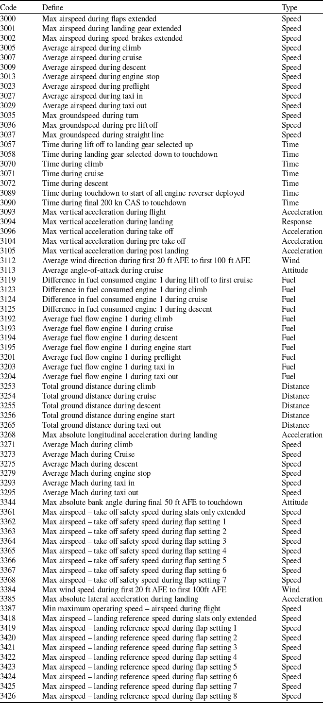
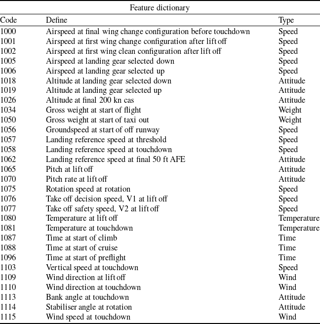
Building on the optimal TL CQR model with A320 as the informative source, we proceed to analyse the factors influencing A380 hard landing risk. The features are divided into several classifications, namely speed, fuel, distance, time, acceleration (non-vertical), weight, attitude, wind speed and temperature. The detailed type of each variable is shown in the ‘type’ column of the Tables A3 and A4.
In order to quantify the impact of different types on the model results, this paper first sums the absolute values of the estimated coefficients of the variables contained in various types of features, and then converts them into relative data with a sum of 1 by normalisation. Finally, the relative contribution value of the type is visualised in Fig. 7 and Table 2. The results show that the controllable factors such as speed, acceleration and attitude have a greater impact on the hard landing risk, while the external conditions such as time, distance, fuel and wind speed have less impact. In summary, the focus of reducing the risk of hard landing is on the optimisation and management of ‘controllable factors’. Reflected in real life, it is necessary to further improve the refined management mechanism of the aircraft control system, improve aircraft performance at the technical level, and strengthen the training of pilots. Reduce the adverse effects of controllable factors from two aspects of human operation and equipment control, thus effectively reducing the risk of the landing phase.
Features contribution from A380 TL CQR with
 $ \tau =\rm{c}(\rm{0.85,0.9,0.95})$

Plot for features contribution from A380 TL CQR with
 $ \tau =c(\rm{0.85,0.9,0.95})$
.

7.0 Summary
In the field of flight safety monitoring, traditional machine learning methods rely on the condition of error distribution, which has limitations when applied to QAR data. Aiming at this application difficulty, we develop a transfer learning framework based on composite quantile regression. By constructing pseudo response variables, the algorithm transforms the non-smooth composite quantile loss into a linear loss form. A large number of numerical simulations show that the algorithm significantly improves the robustness and applicability of the model. In addition, for the case where the informative set in the actual data is unknown, an informative set detection algorithm based on cross-validation is proposed, which can effectively detect the source that can be used for migration. In the QAR data, we establish a composite quantile regression model for the landing risk of the A380 aircraft, and other types of aircraft data can provide additional useful information.
Follow-up research can be extended to other aspects. For example, Li et al. [Reference Li, Cai and Duan23] considered the problem of data privacy, and an extension direction is to study the privacy protection problem in combination with distributed computing, so as to apply to the multi-source situation. The research focus of the example part is QAR data. In the future, it can also be extended to medical, financial and other fields with heterogeneity and heavy-tailed problems to verify the domain applicability of the algorithm.
Acknowledgements
The authors sincerely thank the editor and the anonymous reviewers for their insightful comments and constructive suggestions, which greatly improved the quality of this manuscript. This research is supported by National Natural Science Foundation of China (11771215), Young Talent Fund of Association for Science and Technology in Shaanxi, China (20260518).
Appendix A. Proofs of theorem
The theoretical proof of the convergence rate for CQR is a natural extension of that for the QR case. Consequently, the proof of Theorem 1 follows a structure analogous to that of Theorem 1 in Jin et al. [Reference Jin, Yan and Aseltine9]. The principal technical difficulty lies in dealing with the quantile loss, which we address by introducing a pseudo-response variable following the approach of Chen et al. [Reference Chen, Liu and Mao2]. To maintain a self-contained presentation, we include here the necessary background results from the literature, adapted to our framework. For notational simplicity, we keep the same symbol for constants that appear in convergence rates or probabilistic bounds; for instance,
 $ {c}_{1}$
consistently denotes a generic positive constant in expressions such as
 $ 1-{\exp}\{-\textit{c}_{1}\textit{n}_{0}\}$
. To facilitate the proof, we first establish the convergence rate of the quantile regression estimator under the setting of a single quantile level, and then extend the result to the composite quantile regression estimator with multiple quantile points.
Lemma 1 (Theorem 1 in Jin et al. [Reference Jin, Yan and Aseltine9]). Suppose Conditions 1–6 hold true. We take
 $ {\lambda }_{1}\asymp\sqrt{\log\!(\textit{p}\vee {\rm{m}\rm{a}\rm{x}}_{k\in \mathcal{A}\cup \{0\}}\textit{n}_\textit{k})/(\textit{n}_{\mathcal{A}}+\textit{n}_{0})}$
and
 $ {\lambda }_{0}\asymp{\lambda }_{2}\asymp\sqrt{\log\!(\textit{p}\vee \textit{n}_{0})/\textit{n}_{0}}$
, then with
 \begin{align*} {\xi _1}\left( {{n_0},{n_{\mathcal{A}}},{\mathop{\max }\limits_{k \in {\mathcal{A}} \cup \{ 0\} }}{n_k},{s_0},p} \right) &= {{{s_0}\,\log \left( {p \vee {{\max }_{k \in {\mathcal{A}} \cup \{ 0\} }}{n_k}} \right)} \over {{n_{\mathcal{A}}} + {n_0}}}\nonumber \\ & \quad + {{{s_0}\,\log ( {p \vee {n_0}} )} \over {{n_0}}} \wedge {C_{\boldsymbol {\Sigma }}}d\sqrt {{{\log ( {p \vee {n_0}} )} \over {{n_0}}}} \wedge {\left( {{C_{\boldsymbol {\Sigma }}}d} \right)^2}, \end{align*}
we have
 \begin{align*}{\mathbb{P}} \left( {{1 \over {{n_0}}}{{\left\| {{{\boldsymbol{X}}^{(0)}}({\widehat {{\boldsymbol{\beta}} }} - {{\boldsymbol {\beta }}^{(0)}})} \right\|}^2} \vee {{\left\| {{\widehat {{\boldsymbol{\beta}} }} - {{\boldsymbol {\beta }}^{(0)}}} \right\|}^2} \lesssim {\xi _1}\left( {{n_0},{n_{\mathcal{A}}},{\mathop{\max }\limits_{k \in {\mathcal{A}} \cup \{ 0\} }}{n_k},{s_0},p} \right)} \right)\end{align*}
 \begin{align*} \ge 1 - {C_1}\exp \left( { - {C_2}\mathop {\min }\limits_{k \in {\mathcal{A}} \cup \{0\}} {n_k}} \right) - {C_3}{\left( {\mathop {\min }\limits_{k \in {\mathcal{A}} \cup \{0\}} {n_k}} \right)^{ - {C_4}{{\underline s }_{\mathcal{A}}}}} - \exp \left( { - {C_5}\,\log\,p} \right)\!,\end{align*}
for some positive constants
 $ {C}_{1}$
,…,
 $ {C}_{5}$
, where
 $ {\underline s} _{\mathcal{A}}={\rm{m}\rm{i}\rm{n}}_{k\in \mathcal{A}\cup \{0\}}{s}_{k}$
.
Lemma 2 (Proposition 11 in Chen et al. [Reference Chen, Liu and Mao2]). Denote
 $ {\widehat{\boldsymbol {\Sigma }}}^{(k)}={\sum }_{i=1}^{{n}_{k}} {{\boldsymbol{X}}^{(k)}}^{{\top}}{\boldsymbol{X}}^{(k)}/{n}_{k}$
for
 $ k=0,\dots ,K$
. Recall
 $ {\tilde{\boldsymbol{y}}}^{(k)}$
is the surrogate response. Under Conditions 1, 2, 4, 5 and 6, for any
 $ k=0,\dots ,K$
, we have
 \begin{align*}{\left\| {{1 \over {{n_k}}}{{\boldsymbol{X}}^{{{(k)}^ \top }}}{{{\tilde{\boldsymbol{y}}}}^{(k)}} - {{{\widehat {\boldsymbol\Sigma }}}^{(k)}}{{\boldsymbol {\beta }}^{(k)}}} \right\|_\infty } \lesssim \sqrt {{{\log \left( {p \vee {n_k}} \right)} \over {{n_k}}}} + {{{s_k}\log \left( {p \vee {n_k}} \right)} \over {{n_k}}}.\end{align*}
with probability at least
 $ 1-{c}_{1}{n}_{k}^{-{c}_{2}{s}_{k}}-{c}_{3}{\exp}(\!-\textit{c}_{4}\textit{n}_{\textit{k}})$
for positive constants
 $ {c}_{1}$
to
 $ {c}_{4}$
.
Remark 1. The necessity of Condition 1 can be seen from the following argument. Applying the proof technique of Proposition 11 in Chen et al. [Reference Chen, Liu and Mao2] gives
 \begin{align*} {{\left\| {\frac{1}{n_k}{\boldsymbol{X}^{(k)^\top}}{{\widetilde{\boldsymbol{y}}}^{(k)}} - {\widehat{\boldsymbol {\Sigma}}{}^{(k)}}{\boldsymbol {\beta} ^{(k)}}} \right\|}_\infty } \lesssim \sqrt {\frac{{\log p}}{{{n_k}}}} + \sqrt {\frac{{{s_k}{z_n}\log {n_k}}}{{{n_k}}}} + z_n^2 ,\end{align*}
where
 $ {z}_{n}=\sqrt{{s}_{k}\log {\textit{n}}_{\textit{k}}/{\textit{n}}_{\textit{k}}}$
is the convergence rate of the initial estimator of
 $ {\boldsymbol{\beta }}_{k}$
. Consequently, to attain the rate required in Lemma 1 we must have
 $ {s}_{k}{z}_{n}=O(1)$
, i.e.
 $ \sqrt{{s}_{k}^{3}\log {\textit{n}}_{\textit{k}}/{\textit{n}}_{\textit{k}}}=O(1)$
. This forces
 $ {s}_{k}=O\left({n}_{k}^{b}\right)$
with
 $ b\in (\rm{0,1}/3)$
, which is precisely what Condition 1 states.
 \begin{align} { {\widehat f}^{(k)}}( 0 ) = \frac{1}{{n_k}h^{(k)}}\sum\limits_{i = 1}^{{n_k}} K_h\left(\frac{ y_i^{(k)} - \boldsymbol{x}_i^{(k)^\top}{\widehat{\boldsymbol {\beta}}{} ^{(k)}}}{h^{(k)}}\right)\!,\end{align}
Namely, with
 $ {\widehat{f}}^{(k)}(0)$
defined in 16, Condition 4 contributes to obtain
 \begin{align*} \left| {{{\widehat f}^{(k)}}(0) - {f^{(k)}}(0)} \right| = O_P\left( {\sqrt {\frac{{{s_k}\log {n_k}}}{{{n_k}{h^{(k)}}}}} + \sqrt {\frac{{{s_k}\log {n_k}}}{{{n_k}}}} } \right)\!.\end{align*}
Specifically, denote
 \begin{align*} \mathcal{B}{n,{h^{(k)}}}^{(k)}\left( \boldsymbol {\beta} \right) = \frac{1}{{n{h^{(k)}}}}\sum\limits_{i = 1}^{{n_k}} {K_h\left( {\frac{{y_i^{(k)} - \boldsymbol{x}_{i,{S_k}}^{(k)^\top}{\boldsymbol {\beta} _{{S_k}}}}}{{{h^{(k)}}}}} \right)}, \end{align*}
in which
 $ {\boldsymbol{x}}_{i}^{(k{)}^{{\top}}}{\widehat{\boldsymbol{\beta }}}^{(k)}$
is replaced by
 $ {\boldsymbol{x}}_{i,{S}_{k}}^{(k{)}^{{\top}}}{\boldsymbol{\beta }}_{{S}_{k}}$
. If
 $ {\hat{S}}_{k}\subseteq {S}_{k}$
holds true with high probability (for which we would need the irrepresentable condition), then we have
 $ {\widehat{f}}^{(k)}(0)=\mathcal{B}n,{{h}^{(k)}}^{(k)}({\hat{\boldsymbol{\beta }}}^{(k)})$
with high probability and can bound
 $|{\widehat{f}}^{(k)}(0)-{f}^{(k)}(0)|$
by
 \begin{align*} \left| {{{\widehat f}^{(k)}}(0) - {f^{(k)}}(0)} \right| \le \mathop {\sup }\limits_{\left\| {{\boldsymbol {\beta} _{{S_k}}} - \boldsymbol {\beta} _{{S_k}}^{(k)}} \right\| \le {z_n}} \left| {\mathcal{B}{n,{h^{(k)}}}^{(k)}\left( \boldsymbol {\beta} \right) - {f^{(k)}}(0)} \right|,\end{align*}
where
 $ {z}_{n}=\sqrt{{s}_{k}\log {\textit{n}}_{\textit{k}}/{\textit{n}}_{\textit{k}}}$
is the convergence rate of the initial estimator of
 $ {\boldsymbol{\beta }}_{k}$
provided by Sun et al. [Reference Sun, Zhou and Fan11].
As demonstrated in Chen et al. [Reference Chen, Liu and Mao2], for every coordinate
 $ i$
belonging to the support set
 $ {S}_{k}$
, we partition the interval
 $ [{{\boldsymbol{\beta}} }_{i}^{(k)}-{z}_{n},\rm{}\rm{}{{\boldsymbol{\beta}} }_{i}^{(k)}+{z}_{n}]$
into
 $ {n}^{M}$
small sub-intervals of length
 $ 2{z}_{n}/{n}^{M}$
. In this way, we construct a collection of points
 $ \{{\boldsymbol{\beta }}_{j},1\le j\le {q}_{n}\}$
in
 $ {\mathbb{R}}^{p}$
whose cardinality satisfies
 $ {q}_{n}\le {n}^{M{s}_{k}}$
, and such that for any
 $ \boldsymbol{\beta }$
inside the ball
 $ \| {\boldsymbol{\beta }}_{{S}_{k}}-{\boldsymbol{\beta }}_{{S}_{k}}^{(k)}\| \le {z}_{n}$
there exists an index
 $ j$
(
 $ 1\le j\le {q}_{n}$
) with
 $ \| {\boldsymbol{\beta }}_{{S}_{k}}-{\boldsymbol{\beta }}_{j,{S}_{k}}\| \le 2\sqrt{{s}_{k}}\rm{}\frac{{z}_{n}}{{n}^{M}}$
,
 $ \| {\boldsymbol{\beta }}_{j,{S}_{k}}-{\boldsymbol{\beta }}_{{S}_{k}}^{(k)}\| \le {z}_{n}.$
Consequently, we can relate
 $ {\rm{s}\rm{u}\rm{p}}_{\| {\boldsymbol{\beta }}_{{S}_{k}}-{\boldsymbol{\beta }}_{{S}_{k}}^{(k)}\| \le {z}_{n}}|{\mathcal{B}}_{n,{h}^{(k)}}^{(k)}(\boldsymbol{\beta })-{f}^{(k)}(0\left)\right|$
to
 $ {\rm{s}\rm{u}\rm{p}}_{1\le j\le {n}^{M{s}_{k}}}\left|{\mathcal{B}}_{n,{h}^{(k)}}^{(k)}\right({\boldsymbol{\beta }}_{j})-{f}^{(k)}(0)|,$
and the latter can be bounded using exponential inequalities. This finally yields the required bound on the error of estimating the density functions.
Lemma 3 (Theorem 1 in Raskutti et al. [Reference Raskutti, Wainwright and Yu24]). Denote
 $ {\widehat{\boldsymbol {\Sigma }}}^{\mathcal{A}}={\sum }_{k\in \mathcal{A}\cup \{0\}} {\alpha }_{k}{\widehat{\boldsymbol {\Sigma }}}^{(k)}$
,
 $ {\boldsymbol {\Sigma }}^{\mathcal{A}}={\sum }_{k\in \mathcal{A}\cup \{0\}} {\alpha }_{k}{\boldsymbol {\Sigma }}^{(k)}$
and
 $ {\rho }^{2}(\boldsymbol{\Sigma})=\underset{j=1,\dots ,p}{\rm{m}\rm{a}\rm{x}}{{\Sigma }}_{j,j}$
, where
 $ {\alpha }_{k}=\frac{{n}_{k}}{{n}_{\mathcal{A}}+{n}_{0}}$
. Under Condition 2, we have
 \begin{align*} {u^\top}{\widehat{\boldsymbol {\Sigma}}{} ^\mathcal{A}}u \ge \frac{1}{32}{u^\top}{\boldsymbol {\Sigma} ^\mathcal{A} }u - 81{\rho ^2}\left( \boldsymbol {\Sigma} ^\mathcal{A} \right)\frac{{\log p}}{n_\mathcal{A}+n_0}\left\| u \right\|_1^2\end{align*}
for any
 $ u\in {\mathbb{R}}^{p}$
with probability at least
 $ 1-\exp\!(-{c}_{1}({n}_{\mathcal{A}}+{n}_{0}))$
and
 \begin{align*} {u^\top}{\widehat{\boldsymbol {\Sigma}}{} ^{(0)}}u \ge \frac{1}{32}{u^\top}{\boldsymbol {\Sigma} ^{(0)}}u - 81{\rho ^2}\left( {\boldsymbol {\Sigma} ^{(0)}} \right)\frac{{\log p}}{n_0}\left\| u \right\|_1^2\end{align*}
for any
 $ u\in {\mathbb{R}}^{p}$
with probability at least
 $ 1-{\exp}(\!-{c}_{1}{n}_{0})$
for positive constant
 $ {c}_{1}$
.
Lemma 4 (Bernstein’s inequality (Theorem 1.10 of Boucheron et al. [Reference Boucheron, Lugosi and Bousquet25])). A random variable
 $ X$
is said to follow a sub-exponential distribution with parameter
 $ \lambda $
(written
 $ X\sim \rm{s}\rm{u}\rm{b}\rm{E}\left(\lambda \right)$
) if
 $ \mathbb{E}\left[X\right]=0,$
and its moment generating function satisfies
 \begin{align*}{\mathbb{E}} \left[ {{e^{sX}}} \right] \le \exp \left( {{1 \over 2}{s^2}{\lambda ^2}} \right)\!,\,\,\,\,\,\,\,\forall \left| s \right| \le {1 \over \lambda }.\end{align*}
If
 $ {X}_{1},\dots ,{X}_{n}$
are independent random variables with
 $ \mathbb{E}{X}_{i}={\mu }_{i}$
and
 $ {X}_{i}-{\mu }_{i}\sim subE\left(\lambda \right)$
, then for any
 $ t \gt 0$
we have
 \begin{align*} {\mathbb{P}}\left( {\frac{1}{n}\left| {\sum\limits_{i = 1}^n {\left( {{X_i} - {\mu _i}} \right)} } \right| \ge t} \right) \le \exp \left( { - \frac{n}{2}\min \left\{ {\frac{{{t^2}}}{\lambda ^2},\frac{t}{\lambda}} \right\}} \right)\!.\end{align*}
We now outline the proof of Lemma 1, with the detailed derivations to follow. Let
 $ {\boldsymbol{\beta }}^{\mathcal{A}}$
denote the probabilistic limit of
 $ {\widehat{\boldsymbol{\beta }}}^{\mathcal{A}}$
in Step 3 of the oracle QR algorithm [Reference Jin, Yan and Aseltine9]. It solves the moment equation
 \begin{align} {\mathbb{E}}\left[ {\sum\limits_{k \in {\mathcal{A}} \cup \{0\}} {{{\left( {{\boldsymbol{X}^{(k)}}} \right)}^\top}\left( {{{\tilde y}^{(k)}} - {\boldsymbol{X}^{(k)}}{\boldsymbol {\beta} ^{\mathcal{A}}}} \right)} } \right] = 0,\end{align}
where
 $ {\tilde y}^{(k)}={\boldsymbol{x}}^{(k{)}^{{\top}}}{\boldsymbol{\beta }}^{(k)}-\left\{{f}^{(k)}\right(0\left){\}}^{-1}\right\{I({y}^{(k)}-{\boldsymbol{x}}^{(k{)}^{{\top}}}{\boldsymbol{\beta }}^{(k)}\le 0)-\tau \}.$
Thus,
 $ {\boldsymbol{\beta }}^{\mathcal{A}}$
has the explicit form as
 $ {\boldsymbol{\beta }}^{\mathcal{A}}={\boldsymbol{\beta }}^{(0)}+{\boldsymbol{\delta }}^{\mathcal{A}}$
, where
 $ {\boldsymbol{\delta }}^{\mathcal{A}}=({\boldsymbol {\Sigma }}^{\mathcal{A}}{)}^{-1}{\sum }_{k\in \mathcal{A}\cup \{0\}} {\alpha }_{k}{\boldsymbol {\Sigma }}^{(k)}{\boldsymbol{\delta }}^{(k)}$
. It implies
 $ {\boldsymbol{\beta }}^{\mathcal{A}}$
is a pooled version of
 $ {\boldsymbol{\beta }}^{(0)}$
and
 $ {\boldsymbol{\beta }}^{(k)}$
for all
 $ k\in \mathcal{A}$
such that
 $ {\boldsymbol{\beta }}^{\mathcal{A}}=({\boldsymbol {\Sigma }}^{\mathcal{A}}{)}^{-1}{\sum }_{k\in \mathcal{A}\cup \{0\}} {\alpha }_{k}{\boldsymbol {\Sigma }}^{(k)}{\boldsymbol{\beta }}^{(k)}$
.
Define
 \begin{align*}{B_1} &= {\mkern 1mu} {\rm{ }}\left\{ {{1 \over {{n_{\mathcal{A}}} + {n_0}}}{{\left\| {\sum\limits_{k \in {\mathcal{A}} \cup \{0\}} {{{\boldsymbol{X}}^{{{(k)}^ \top }}}({{{\tilde{\boldsymbol{y}}}}^{(k)}} - {{\boldsymbol{X}}^{(k)}}{{\boldsymbol {\beta }}^{\mathcal{A}}})} } \right\|}_\infty } \le {{{\lambda _1}} \over 2}} \right\}\!,\\{B_2} &= {\mkern 1mu} \left\{ {{1 \over {{n_0}}}{{\left\| {{{\boldsymbol{X}}^{{{(0)}^ \top }}}\left( {{{\tilde y}^{(0)}} - {{\boldsymbol{X}}^{(0)}}{{\boldsymbol {\beta }}^{(0)}}} \right)} \right\|}_\infty } \le {{{\lambda _2}} \over 2}} \right\}\!.\end{align*}
We will show the following statements:
-
• (1) Denote
$ {\widehat{\boldsymbol{u}}}^{\mathcal{A}}={\widehat{\boldsymbol{\beta }}}^{\mathcal{A}}-{\boldsymbol{\beta }}^{\mathcal{A}}$
. On the event of
$ {B}_{1}$
, we havewith probability at least
\begin{align*}{{\widehat{\boldsymbol{u}}}^{{{\mathcal{A}}^ \top }}}{{\widehat {\boldsymbol\Sigma }}^{\mathcal{A}}}{{\widehat{\boldsymbol{u}}}^{\mathcal{A}}} \vee &{\left\| {{{{\widehat{\boldsymbol{u}}}}^{\mathcal{A}}}} \right\|^2}\lesssim {s_0}\lambda _1^2 + {\lambda _1}{C_{\boldsymbol {\Sigma }}}d,\\&{\left\| {{{{\widehat{\boldsymbol{u}}}}^{\mathcal{A}}}} \right\|_1}\lesssim {s_0}{\lambda _1} + {C_{\boldsymbol {\Sigma }}}d\end{align*}
$ 1-{\exp}(\!-{c}_{1}({n}_{\mathcal{A}}+{n}_{0}))$
.
-
• (2) Denote
$ {\widehat{\boldsymbol{v}}}^{\mathcal{A}}={\widehat{\boldsymbol{\delta }}}^{\mathcal{A}}-{\boldsymbol{\delta }}^{\mathcal{A}}$
. On the event of
$ {B}_{2}$
, we havewith probability at least
\begin{align*}&{{\widehat{\boldsymbol{u}}}^{{{\mathcal{A}}^ \top }}}{{\widehat {\boldsymbol\Sigma }}^{(0)}}{{\widehat{\boldsymbol{u}}}^{\mathcal{A}}} \vee {\left\| {{{{\widehat{\boldsymbol{v}}}}^{\mathcal{A}}}} \right\|^2}\lesssim {s_0}\lambda _1^2 + {\lambda _1}{C_{\boldsymbol {\Sigma }}}d,\\&{{\widehat{\boldsymbol{v}}}^{\mathcal{A}^{\top}}} {{\widehat {\boldsymbol\Sigma }}^{(0)}}{{\widehat{\boldsymbol{v}}}^{\mathcal{A}}}\lesssim {\lambda _2}{C_{\boldsymbol {\Sigma }}}d,\\&{\left\| {{{{\widehat{\boldsymbol{v}}}}^{\mathcal{A}}}} \right\|^2}\lesssim {\lambda _2}{C_{\boldsymbol {\Sigma }}}d \wedge {\left( {{C_{\boldsymbol {\Sigma }}}d} \right)^2}\end{align*}
$ 1-3\,{\exp}(\!-{c}_{1}{n}_{0})$
.


We then show that
 $ \mathbb{P}\left({B}_{1}\cap {B}_{2}\right)\to 1$
as
 $ p\to \rm{\infty }$
and
 $ \underset{k\in \mathcal{A}\cup \{0\}}{\rm{m}\rm{i}\rm{n}}{n}_{k}\to \rm{\infty }$
, which is the minimum sample size across the informative sources and the target. Finally, the proof of Lemma 1 is proved by appealing to Lemma 3 together with the observation that
 \begin{align*} \left\| {\widehat{\boldsymbol {\beta}}{} - {\boldsymbol {\beta} ^{(0)}}} \right\| = \left\| {\left( {{\widehat{\boldsymbol {\beta}}{} ^\mathcal{A}} - {\boldsymbol {\beta} ^\mathcal{A}}} \right) - \left( {{\widehat{\boldsymbol {\delta}}{}^\mathcal{A}} - {\boldsymbol {\delta} ^\mathcal{A}}} \right)} \right\|\le\|\widehat{\boldsymbol{u}}^{\mathcal{A}}\|+\|\widehat{\boldsymbol{v}}^{\mathcal{A}}\|.\end{align*}
We now proceed to prove statement (1). The following oracle inequality is identical to (A.1) in the supplementary material of Li et al. [Reference Li, Cai and Li7]. Expanding the loss function in Step 3 of the oracle QR algorithm in Jin et al. [Reference Jin, Yan and Aseltine9] via Taylor expansion gives
 \begin{align*}&\quad {1 \over 2}{{\widehat{\boldsymbol{u}}}^{{{\mathcal{A}}^ \top }}}{{\widehat {\boldsymbol\Sigma }}^{\mathcal{A}}}{{\widehat{\boldsymbol{u}}}^{\mathcal{A}}}\\& \le {\lambda _1}{\big\| {{{\boldsymbol {\beta }}^{\mathcal{A}}}} \big\|_1} - {\lambda _1}{\big\| {{{{\widehat {{\boldsymbol{\beta}} }}}^{\mathcal{A}}}} \big\|_1} + \left| {{{{{{\widehat{\boldsymbol{u}}}}^{{{\mathcal{A}}^ \top }}}} \over {\left( {{n_{\mathcal{A}}} + {n_0}} \right)}}\sum\limits_{k \in {\mathcal{A}} \cup \{0\}} {{{\boldsymbol{X}}^{{{(k)}^ \top }}}\left( {{{{\tilde{\boldsymbol{y}}}}^{(k)}} - {{\boldsymbol{X}}^{(k)}}{{\boldsymbol {\beta }}^{\mathcal{A}}}} \right)} } \right|\\& \le {\lambda _1}{\big\| {{{\boldsymbol {\beta }}^{\mathcal{A}}}} \big\|_1} - {\lambda _1}{\big\| {{{{\widehat {{\boldsymbol{\beta}} }}}^{\mathcal{A}}}} \big\|_1} + {{{\lambda _1}} \over 2}{\big\| {{\hat{\boldsymbol{u}}^{\mathcal{A}}}} \big\|_1}\\ & \le {3 \over 2}{\lambda _1}{\big\| {{\widehat{\boldsymbol{u}}}_{{S_0}}^{\mathcal{A}}} \big\|_1} + {\lambda _1}{\big\| {{\boldsymbol {\beta }}_{{S_0}^c}^{\mathcal{A}}} \big\|_1} - {\lambda _1}{\big\| {{\widehat {{\boldsymbol{\beta}} }}_{{S_0}^c}^{\mathcal{A}}} \big\|_1} + {1 \over 2}{\lambda _1}{\big\| {{\widehat{\boldsymbol{u}}}_{S_0^c}^{\mathcal{A}}} \big\|_1}\\ & \le {3 \over 2}{\lambda _1}{\big\| {{\widehat{\boldsymbol{u}}}_{{S_0}}^{\mathcal{A}}} \big\|_1} + {3 \over 2}{\lambda _1}{\big\| {{\boldsymbol {\beta }}_{{S_0}^c}^{\mathcal{A}}} \big\|_1} - {1 \over 2}{\lambda _1}{\big\| {{\widehat{\boldsymbol{u}}}_{{S_0}^c}^{\mathcal{A}}} \big\|_1}.\end{align*}
-
(1) If
$ \| {\widehat{\boldsymbol{u}}}_{{S}_{0}}^{\mathcal{A}}{\| }_{1}\ge \| {\boldsymbol{\beta }}_{{{S}_{0}}^{c}}^{\mathcal{A}}{\| }_{1}$
, with a positive constant
$ {c}_{4}$
, we can further havewhere the first line holds true with probability at least
\begin{align*}{\left\| {{{{\widehat{\boldsymbol{u}}}}^{\mathcal{A}}}} \right\|^2} - {{\log p} \over {{n_{\mathcal{A}}} + {n_0}}}\left\| {{{{\widehat{\boldsymbol{u}}}}^{\mathcal{A}}}} \right\|_1^2 &\lesssim {1 \over 2}{{\widehat{\boldsymbol{u}}}^{{{\mathcal{A}}^ \top }}}{{\widehat {\boldsymbol\Sigma }}^{\mathcal{A}}}{{\widehat{\boldsymbol{u}}}^{\mathcal{A}}}\\& \le 3{\lambda _1}{\left\| {{\widehat{\boldsymbol{u}}}_{{S_0}}^{\mathcal{A}}} \right\|_1} - {1 \over 2}{\lambda _1}{\left\| {{\widehat{\boldsymbol{u}}}_{{S_0}^c}^{\mathcal{A}}} \right\|_1}\\ & \le 3{\lambda _1}{\left\| {{\widehat{\boldsymbol{u}}}_{{S_0}}^{\mathcal{A}}} \right\|_1}\\ & \le 3{\lambda _1}\sqrt {{s_0}} \left\| {\hat{\boldsymbol{u}}_{{S_0}}^{\mathcal{A}}} \right\|\\ & \le 3{\lambda _1}\sqrt {{s_0}} \left\| {{{{\widehat{\boldsymbol{u}}}}^{\mathcal{A}}}} \right\|\!,\end{align*}
$ 1-{\exp}(\!-{c}_{1}({n}_{\mathcal{A}}+{n}_{0}))$
due to Lemma 3 and Condition 4. It further leads to(18)
\begin{align}{\left\| {{{{\widehat{\boldsymbol{u}}}}^{\mathcal{A}}}} \right\|^2} \lesssim {s_0}\lambda _1^2,\end{align}
(19)by utilising
\begin{align}{\left\| {{{{\widehat{\boldsymbol{u}}}}^{\mathcal{A}}}} \right\|_1} \lesssim {s_0}{\lambda _1}\end{align}
$ {s}_{0}\log p/({n}_{\mathcal{A}}+{n}_{0})=o(1)$
derived from Condition 3.
-
(2) If
$ \| {\widehat{\boldsymbol{u}}}_{{S}_{0}}^{\mathcal{A}}{\| }_{1}\le \| {\boldsymbol{\beta }}_{{{S}_{0}}^{c}}^{\mathcal{A}}{\| }_{1}$
, we have
\begin{align*}0 \le {1 \over 2}{{\widehat{\boldsymbol{u}}}^{{{\mathcal{A}}^ \top }}}{{\widehat {\boldsymbol\Sigma }}^{\mathcal{A}}}{{\widehat{\boldsymbol{u}}}^{\mathcal{A}}} \le 3{\lambda _1}{\left\| {{\boldsymbol {\beta }}_{{S_0}^c}^{\mathcal{A}}} \right\|_1} - {1 \over 2}{\lambda _1}{\left\| {{\widehat{\boldsymbol{u}}}_{{S_0}^c}^{\mathcal{A}}} \right\|_1}.\end{align*}


It follows that
 \begin{align*}{\left\| {{\widehat{\boldsymbol{u}}}_{{S_0}^c}^{\mathcal{A}}} \right\|_1} \le 6{\left\| {{\boldsymbol {\beta }}_{{S_0}^c}^{\mathcal{A}}} \right\|_1},\end{align*}
and
 \begin{align}{\left\| {{{{\widehat{\boldsymbol{u}}}}^{\mathcal{A}}}} \right\|_1} = {\left\| {{\widehat{\boldsymbol{u}}}_{{S_0}}^{\mathcal{A}}} \right\|_1} + {\left\| {{\widehat{\boldsymbol{u}}}_{{S_0}^c}^{\mathcal{A}}} \right\|_1} \le 7{\left\| {{\boldsymbol {\beta }}_{{S_0}^c}^{\mathcal{A}}} \right\|_1} \le 7{\left\| {{\boldsymbol {\delta }}_{{S_0}^c}^{\mathcal{A}}} \right\|_1} \le 7{C_{\boldsymbol {\Sigma }}}d.\end{align}
This implies
 $ \| {\widehat{\boldsymbol{u}}}^{\mathcal{A}}\| \le 7{C}_{\boldsymbol {\Sigma }}d$
by the
 $ {\ell}_{1}$
-
 $ {\ell}_{2}$
inequality. By Lemma 3, we have
 \begin{align*}{\left\| {{{{\widehat{\boldsymbol{u}}}}^{\mathcal{A}}}} \right\|^2} - {{\log p} \over {{n_{\mathcal{A}}} + {n_0}}}\left\| {{{{\widehat{\boldsymbol{u}}}}^{\mathcal{A}}}} \right\|_1^2 &\lesssim {1 \over 2}{{\widehat{\boldsymbol{u}}}^{{{\mathcal{A}}^ \top }}}{{\widehat {\boldsymbol\Sigma }}^{\mathcal{A}}}{{\widehat{\boldsymbol{u}}}^{\mathcal{A}}}\\ &\le 3{\lambda _1}{\left\| {{\boldsymbol {\beta }}_{{S_0}^c}^{\mathcal{A}}} \right\|_1} - {1 \over 2}{\lambda _1}{\left\| {{\widehat{\boldsymbol{u}}}_{{S_0}^c}^{\mathcal{A}}} \right\|_1}\\ &\le 3{\lambda _1}{\left\| {{\boldsymbol {\beta }}_{{S_0}^c}^{\mathcal{A}}} \right\|_1}\\ &\le 3{\lambda _1}{C_{\boldsymbol {\Sigma }}}d\end{align*}
with probability at least
 $ 1-{\exp}(\!-{c}_{1}({n}_{\mathcal{A}}+{n}_{0}))$
. Noticing that
 $ {C}_{\boldsymbol {\Sigma }}d\sqrt{\log p/({n}_{A}+{n}_{0})}=o(1)$
as derived from Condition 3, we get
 \begin{align*}{\left\| {{{{\widehat{\boldsymbol{u}}}}^{\mathcal{A}}}} \right\|^2} &\le {\mkern 1mu} {{\log p} \over {{n_{\mathcal{A}}} + {n_0}}}\left\| {{{{\widehat{\boldsymbol{u}}}}^{\mathcal{A}}}} \right\|_1^2 + 3{\lambda _1}{C_{\boldsymbol {\Sigma }}}d\\ &\le {{\sqrt {{s_0}} \log p} \over {{n_{\mathcal{A}}} + {n_0}}}{\left\| {{{{\widehat{\boldsymbol{u}}}}^{\mathcal{A}}}} \right\|^2} + 3{\lambda _1}{C_{\boldsymbol {\Sigma }}}d,\end{align*}
and then we have
 \begin{align} {\left\| {\widehat{\boldsymbol{u}}{}^\mathcal{A}} \right\|^2} \lesssim {{\lambda _1}C_{\boldsymbol {\Sigma}} d}.\end{align}
Statement (1) then follows by combining the results from Equations (18), (19), (20) and (21) together with Lemma 3.
We now turn to statement (2). Conditional on the event
 $ {B}_{2}$
, the following oracle inequality holds, which is identical to the one appearing in the proofs of Theorems 1 and 4 in Li et al. [Reference Li, Cai and Li7]. Expanding the loss of
 $ {\widehat{\boldsymbol{\delta }}}^{\mathcal{A}}$
via Taylor expansion gives
 \begin{align*}&\quad {1 \over 2}{{\widehat{\boldsymbol{v}}}^{{{\mathcal{A}}^ \top }}}{{\widehat {\boldsymbol\Sigma }}^{(0)}}{{\widehat{\boldsymbol{v}}}^{\mathcal{A}}}\\&\le {\lambda _2}{\big\| {{{\boldsymbol {\delta }}^{\mathcal{A}}}} \big\|_1} - {\lambda _2}{\big\| {{{{\widehat{\boldsymbol \delta }}}^{\mathcal{A}}}} \big\|_1} + \left| {{{{{{\widehat{\boldsymbol{v}}}}^{{{\mathcal{A}}^ \top }}}} \over {{n_0}}}{{\boldsymbol{X}}^{{{(0)}^ \top }}}\big\{ {{{{\tilde{\boldsymbol{y}}}}^{(0)}} - {{\boldsymbol{X}}^{(0)}}\big({{{{\widehat {{\boldsymbol{\beta}} }}}^{\mathcal{A}}} - {{\boldsymbol {\delta }}^{\mathcal{A}}}}\big)}\big\}} \right|\\ &= {\lambda _2}{\big\| {{{\boldsymbol {\delta }}^{\mathcal{A}}}} \big\|_1} - {\lambda _2}{\big\| {{{{\widehat{\boldsymbol \delta }}}^{\mathcal{A}}}} \big\|_1} + \left| {{{{{{\widehat{\boldsymbol{v}}}}^{{{\mathcal{A}}^ \top }}}} \over {{n_0}}}{{\boldsymbol{X}}^{{{(0)}^ \top }}}\big\{ {{{{\tilde{\boldsymbol{y}}}}^{(0)}} - {{\boldsymbol{X}}^{(0)}}{{\boldsymbol {\beta }}^{(0)}} - {{\boldsymbol{X}}^{(0)}}\big({{{{\widehat {{\boldsymbol{\beta}} }}}^{\mathcal{A}}} - {{\boldsymbol {\delta }}^{\mathcal{A}}} - {{\boldsymbol {\beta }}^{(0)}}}\big)}\big\}}\right|\\ & = {\lambda _2}{\big\| {{{\boldsymbol {\delta }}^{\mathcal{A}}}} \big\|_1} - {\lambda _2}{\big\| {{{{\widehat{\boldsymbol \delta }}}^{\mathcal{A}}}} \big\|_1} + \left| {{{{{\boldsymbol{v}}^{{{\mathcal{A}}^ \top }}}} \over {{n_0}}}{{\boldsymbol{X}}^{{{(0)}^ \top }}}\big\{ {\big( {{{{\tilde{\boldsymbol{y}}}}^{(0)}} - {{\boldsymbol{X}}^{(0)}}{{\boldsymbol {\beta }}^{(0)}}}\big) - {{\boldsymbol{X}}^{(0)}}{{{\widehat{\boldsymbol{u}}}}^{\mathcal{A}}}}\big\}} \right|\\ & \le {\lambda _2}{\big\| {{{\boldsymbol {\delta }}^{\mathcal{A}}}} \big\|_1} - {\lambda _2}{\big\| {{{{\widehat{\boldsymbol \delta }}}^{\mathcal{A}}}} \big\|_1} + {{{\lambda _2}} \over 2}{\big\| {{{{\widehat{\boldsymbol{v}}}}^{\mathcal{A}}}} \big\|_1} + {{\widehat{\boldsymbol{u}}}^{{{\mathcal{A}}^ \top }}}{{\widehat {\boldsymbol\Sigma }}^{(0)}}{{\widehat{\boldsymbol{u}}}^{\mathcal{A}}} + {1 \over 4}{{\widehat{\boldsymbol{v}}}^{{{\mathcal{A}}^ \top }}}{{\widehat {\boldsymbol\Sigma }}^{(0)}}{{\widehat{\boldsymbol{v}}}^{\mathcal{A}}}.\end{align*}
Hence, by noticing
 $ \| {\widehat{\boldsymbol{v}}}^{\mathcal{A}}{\| }_{1}=\| {\widehat{\boldsymbol{\delta }}}^{\mathcal{A}}-{\boldsymbol{\delta }}^{\mathcal{A}}{\| }_{1}\ge \| {\widehat{\boldsymbol{\delta }}}^{\mathcal{A}}{\| }_{1}-\| {\boldsymbol{\delta }}^{\mathcal{A}}{\| }_{1}$
, we have
 \begin{align*}{1 \over 4}{{\widehat{\boldsymbol{v}}}^{{{\mathcal{A}}^ \top }}}{{\widehat {\boldsymbol\Sigma }}^{(0)}}{{\widehat{\boldsymbol{v}}}^{\mathcal{A}}} \le 2{\lambda _2}{\left\| {{{\boldsymbol {\delta }}^{\mathcal{A}}}} \right\|_1} - {{{\lambda _2}} \over 2}{\left\| {{{{\widehat{\boldsymbol{v}}}}^{\mathcal{A}}}} \right\|_1} + {{\widehat{\boldsymbol{u}}}^{{{\mathcal{A}}^ \top }}}{{\widehat {\boldsymbol\Sigma }}^{(0)}}{{\widehat{\boldsymbol{u}}}^{\mathcal{A}}}.\end{align*}
-
(1) If
$ {\widehat{\boldsymbol{u}}}^{{\mathcal{A}}^{{\top}}}{\widehat{\boldsymbol {\Sigma }}}^{(0)}{\widehat{\boldsymbol{u}}}^{\mathcal{A}}\le {\lambda }_{2}\| {\boldsymbol{\delta }}^{\mathcal{A}}{\| }_{1}$
, then(22)which further leads to
\begin{align}0 \le {1 \over 4}{{\widehat{\boldsymbol{v}}}^{{{\mathcal{A}}^ \top }}}{{\widehat {\boldsymbol\Sigma }}^{(0)}}{{\widehat{\boldsymbol{v}}}^{\mathcal{A}}} &\le 3{\lambda _2}{\left\| {{{\boldsymbol {\delta }}^{\mathcal{A}}}} \right\|_1} - {{{\lambda _2}} \over 2}{\left\| {{{{\widehat{\boldsymbol{v}}}}^{\mathcal{A}}}} \right\|_1}\nonumber \\ & \le {\mkern 1mu} \,3{\lambda _2}{\left\| {{{\boldsymbol {\delta }}^{\mathcal{A}}}} \right\|_1}\\ & \le 3{\lambda _2}{C_{\boldsymbol {\Sigma }}}d,\nonumber \end{align}
$ \| {\widehat{\boldsymbol{v}}}^{\mathcal{A}}{\| }_{1}\le 6\| {\boldsymbol{\delta }}^{\mathcal{A}}{\| }_{1}\le 6{C}_{\boldsymbol {\Sigma }}d$
and(23)
\begin{align} \left\| {\widehat{\boldsymbol{v}}{}^\mathcal{A}} \right\| \le \left\| {\widehat{\boldsymbol{v}}{}^\mathcal{A}} \right\|_1 \le 6C_{\boldsymbol {\Sigma}} d.\end{align}
Meanwhile, from Lemma 3, we have
with probability at least
\begin{align*}{\left\| {{{{\widehat{\boldsymbol{v}}}}^{\mathcal{A}}}} \right\|^2} - {{\log p} \over {{n_0}}}\left\| {{{{\widehat{\boldsymbol{v}}}}^{\mathcal{A}}}} \right\|_1^2 &\lesssim {1 \over 4}{{\widehat{\boldsymbol{v}}}^{{{\mathcal{A}}^ \top }}}{{\widehat {\boldsymbol\Sigma }}^{(0)}}{{\widehat{\boldsymbol{v}}}^{\mathcal{A}}}\\ &\le 3{\lambda _2}{\left\| {{{\boldsymbol {\delta }}^{\mathcal{A}}}} \right\|_1}\\ & \le 3{\lambda _2}{C_{\boldsymbol {\Sigma }}}d,\end{align*}
$ 1-{\exp}(\!-{c}_{1}{n}_{0})$
, and then(24)by noticing
\begin{align} {\left\| {\widehat{\boldsymbol{v}}{}^\mathcal{A}} \right\|^2} \lesssim {\lambda _2}C_{\boldsymbol {\Sigma}} d\end{align}
$ {C}_{\boldsymbol {\Sigma }}d(\!\log\!(p\vee {n}_{0})/{n}_{0})^{1/2}=o(1)$
as derived from Condition 3.
-
(2) If
$ {\widehat{\boldsymbol{u}}}^{{\mathcal{A}}^{{\top}}}{\widehat{\boldsymbol {\Sigma }}}^{(0)}{\widehat{\boldsymbol{u}}}^{\mathcal{A}}\ge {\lambda }_{2}\| {\boldsymbol{\delta }}^{\mathcal{A}}{\| }_{1}$
, we have
\begin{align*} 0 \le \frac{1}{4}\widehat{\boldsymbol{v}}{}^{\mathcal{A}^\top}{\widehat{\boldsymbol {\Sigma}}{}^{(0)}}\widehat{\boldsymbol{v}}{}^{\mathcal{A}} \le { 3{\widehat{\boldsymbol{u}}{}^{\mathcal{A}^\top}} }{\widehat{\boldsymbol {\Sigma}}{}^{(0)}}\widehat{\boldsymbol{u}}{}^{\mathcal{A}} - \frac{{{\lambda _2}}}{2}\left\|\widehat{\boldsymbol{v}}{}^{\mathcal{A}}\right\|_1.\end{align*}


It follows that
 \begin{align}{\left\| {{{{\widehat{\boldsymbol{v}}}}^{\mathcal{A}}}} \right\|_1}& \leq \frac{6}{\delta_{2}}\widehat{\boldsymbol{u}}^{\mathcal{A}\,\top}\widehat{\Sigma}^{(0)}\widehat{\boldsymbol{u}}^{\mathcal{A}} \nonumber \\&\lesssim {{{{\left\| {{{{\widehat{\boldsymbol{u}}}}^{\mathcal{A}}}} \right\|}^2}} \over {{\lambda _2}}}\\&\lesssim {{{s_0}\lambda _1^2 + {\lambda _1}{C_{\boldsymbol {\Sigma }}}d} \over {{\lambda _2}}}\nonumber\end{align}
with probability at least
 $ 1-2\,{\exp}(\!-{c}_{1}{n}_{0})$
, where the second line holds true with probability at least
 $ 1-{\exp}(\!-{c}_{1}{n}_{0})$
due to Theorem 1.6 of Zhou [Reference Zhou26], and the third line holds true with probability at least
 $ 1-{\exp}(\!-{c}_{1}({n}_{\mathcal{A}}+{n}_{0}))$
due to (18) and (21). By Lemma 3 and Theorem 1.6 of Zhou [Reference Zhou26], once again, we have
 \begin{align*}{\left\| {{{{\widehat{\boldsymbol{v}}}}^{\mathcal{A}}}} \right\|^2} - {{\log p} \over {{n_0}}}\left\| {{{{\widehat{\boldsymbol{v}}}}^{\mathcal{A}}}} \right\|_1^2 &\lesssim {1 \over 4}{{\widehat{\boldsymbol{v}}}^{{{\mathcal{A}}^ \top }}}{{\widehat {\boldsymbol\Sigma }}^{(0)}}{{\widehat{\boldsymbol{v}}}^{\mathcal{A}}}\\ &\le 3{{\widehat{\boldsymbol{u}}}^{{{\mathcal{A}}^ \top }}}{{\widehat {\boldsymbol\Sigma }}^{(0)}}{{\widehat{\boldsymbol{u}}}^{\mathcal{A}}}\\ &\lesssim {\left\| {{{{\widehat{\boldsymbol{u}}}}^{\mathcal{A}}}} \right\|^2}\\ &\lesssim {s_0}\lambda _1^2 + {\lambda _1}{C_{\boldsymbol {\Sigma }}}d\end{align*}
with probability at least
 $ 1-3\,{\exp}(\!-{c}_{1}{n}_{0})$
. Thus, from (25) that shows
 $ \| {\widehat{\boldsymbol{v}}}^{\mathcal{A}}{\| }_{1}^{2}\log p/{n}_{0}\le ({\lambda }_{2}\| {\widehat{\boldsymbol{v}}}^{\mathcal{A}}{\| }_{1}{)}^{2}=o(1)$
, we have
 \begin{align} {\widehat{\boldsymbol{u}}{}^{\mathcal{A}^\top}}{\widehat{\boldsymbol {\Sigma}}{}^{(0)}}{\widehat{\boldsymbol{u}}{}^{\mathcal{A}}} \vee {\left\| {{\widehat{\boldsymbol{v}}{}^\mathcal{A}}} \right\|^2} \lesssim {{s_0}\lambda _1^2 + {\lambda _1}C_{\boldsymbol {\Sigma}} d}.\end{align}
Statement (2) is established by combining results from (22), (23), (24), (25) and (26).
We now prove that
 $ \mathbb{P}({B}_{1}\cap {B}_{2})\ge 1-{c}_{1}(\underset{k\in \mathcal{A}\cup \{0\}}{\rm{m}\rm{i}\rm{n}}{n}_{k}{)}^{-{c}_{2}{\underline s} _{\mathcal{A}}}-{c}_{3}\,{\exp}(\!-{c}_{4}\underset{k\in \mathcal{A}\cup \{0\}}{\rm{m}\rm{i}\rm{n}}{n}_{k})-{\exp}(\!-{c}_{5}\log p)$
for some positive constants
 $ {c}_{1}$
to
 $ {c}_{5}$
. We utilise the inequality
 $ \mathbb{P}({B}_{1}\cap {B}_{2})\ge \mathbb{P}({B}_{1})+\mathbb{P}\left({B}_{2}\right)-1$
and then bound
 $ \mathbb{P}({B}_{1})$
and
 $ \mathbb{P}\left({B}_{2}\right)$
separately. For
 $ \mathbb{P}\left({B}_{2}\right)$
, we have
 $ \mathbb{P}\left({B}_{2}\right)\ge 1-{c}_{1}{n}_{0}^{-{c}_{2}{s}_{0}}-{c}_{3}\,{\exp}(\!-{c}_{4}{n}_{0})$
by Lemma 2. For
 $ \mathbb{P}({B}_{1})$
, we bound it by the following decomposition:
 \begin{align*}&\quad {1 \over {{n_A} + {n_0}}}{\left\| {\sum\limits_{k \in {{\mathcal{A}}} \cup \{0\}} {{X^{{{(k)}^ \top }}}({{\tilde y}^{(k)}} - {X^{(k)}}{{\boldsymbol{\beta}} ^{\mathcal{A}}})} } \right\|_\infty }\\& = \left\| {\rm{\;}}{1 \over {{n_{\mathcal{A}}} + {n_0}}}\mathop \sum \limits_{k \in {\mathcal{A}} \cup \{0\}} {{\boldsymbol{X}}^{{{(k)}^{\top}}}}{{\tilde{\boldsymbol{y}}}^{(k)}} - \mathop \sum \limits_{k \in {\mathcal{A}} \cup \{0\}} {\alpha _k}{{\widehat {\boldsymbol\Sigma }}^{(k)}}{{\boldsymbol{\beta}} ^{(k)}} + \mathop \sum \limits_{k \in {\mathcal{A}} \cup \{0\}} {\alpha _k}{{\widehat {\boldsymbol\Sigma }}^{(k)}}{{\boldsymbol{\beta}} ^{(k)}} - {{\widehat {\boldsymbol\Sigma }}^{\mathcal{A}}}{{\boldsymbol{\beta}} ^{\mathcal{A}}}\right\|_\infty \\ & = \left\|{\rm{\;}}\mathop \sum \limits_{k \in {\mathcal{A}} \cup \{0\}} {\alpha _k}\left( {{1 \over {{n_k}}}{{\boldsymbol{X}}^{{{(k)}^{\top}}}}{{{\tilde{\boldsymbol{y}}}}^{(k)}} - {{{\widehat {\boldsymbol\Sigma }}}^{(k)}}{{\boldsymbol{\beta}} ^{(k)}}} \right) + \mathop \sum \limits_{k \in {\mathcal{A}} \cup \{0\}} {\alpha _k}\big({{{{\widehat {\boldsymbol\Sigma }}}^{(k)}} - {{\boldsymbol {\Sigma }}^{(k)}}}\big){\delta ^{(k)}} - \big( {{{{\widehat {\boldsymbol\Sigma }}}^{\mathcal{A}}} - {{\boldsymbol {\Sigma }}^{\mathcal{A}}}} \big){\delta ^{\mathcal{A}}}\right\|_\infty \\ & \le \left\| \mathop \sum \limits_{k \in {\mathcal{A}} \cup \{0\}} {\alpha _k}\left( {{1 \over {{n_k}}}{{\boldsymbol{X}}^{{{(k)}^{\top}}}}{{{\tilde{\boldsymbol{y}}}}^{(k)}} - {{{\widehat {\boldsymbol\Sigma }}}^{(k)}}{{\boldsymbol{\beta}} ^{(k)}}} \right)\right\|_\infty + \left\|\mathop \sum \limits_{k \in {\mathcal{A}} \cup \{0\}} {\alpha _k}\big( {{{{\widehat {\boldsymbol\Sigma }}}^{(k)}} - {{\boldsymbol {\Sigma }}^{(k)}}} \big){\delta ^{(k)}}\right\|_\infty \\ & \quad + \left\| \big({{{{\widehat {\boldsymbol\Sigma }}}^{\mathcal{A}}} - {{\boldsymbol {\Sigma }}^{\mathcal{A}}}}\big){\delta ^{\mathcal{A}}}\right\|_\infty \\ & \mathop = \limits^{{\rm{def}}} {\rm{\;}}{D_1} + {D_2} + {D_3}{\rm{\;}}.\end{align*}
For
 $ {D}_{1}$
, based on Lemma 2, we have
 \begin{align*}{\alpha _k}\left\|{1 \over {{n_k}}}{{\boldsymbol{X}}^{{{(k)}^{\top}}}}{{\tilde{\boldsymbol{y}}}^{(k)}} - {{\widehat {\boldsymbol\Sigma }}^{(k)}}{{\boldsymbol{\beta}} ^{(k)}}\right\|_\infty &\lesssim {{{n_k}} \over {{n_{\mathcal{A}}} + {n_0}}}\left( {\sqrt {{{{\rm{log}}\left( {p \vee {n_k}} \right)} \over {{n_k}}}} + {{{s_k}\,{\rm{log}}\left( {p \vee {n_k}} \right)} \over {{n_k}}}} \right)\\&\lesssim {{\sqrt {{n_k}\log \left( {p \vee {n_k}} \right)} } \over {{n_{\mathcal{A}}} + {n_0}}} + {{{s_k}\log \left( {p \vee {n_k}} \right)} \over {{n_{\mathcal{A}}} + {n_0}}}\\&\lesssim {{\sqrt {{n_k}\log \left( {p \vee {n_k}} \right)} } \over {{n_{\mathcal{A}}} + {n_0}}}\\&\lesssim \sqrt {{{\log \left( {p \vee {n_k}} \right)} \over {{n_{\mathcal{A}}} + {n_0}}}} \end{align*}
for any
 $ k\in \mathcal{A}\cup \{0\}$
with probability at least
 $ 1-{c}_{1}{n}_{k}^{-{c}_{2}{s}_{k}}-{c}_{3}\,{\exp}(\!-{c}_{4}{n}_{k})$
, where the third line holds true due to
 $ {s}_{k}=O({n}_{k}^{b})$
with
 $ 0\lt b\lt 1/3$
from Condition 1. Hence, considering that
 $ \left|\mathcal{A}\right|$
is bounded, we have
 \begin{align} {D_1} {}\lesssim \mathop {\max }\limits_{k \in \mathcal{A} \cup \{0\}} \sqrt {\frac{{\log \left( p \vee {n_k} \right)}}{{{n_\mathcal{A}} + {n_0}}}} {}\lesssim \sqrt {\frac{{\log \left( p \vee {{n_{\mathcal{A}}}^*} \right)}}{{{n_\mathcal{A}} + {n_0}}}} \end{align}
with probability at least
 $ 1-{c}_{1}\underset{k\in \mathcal{A}\cup \{0\}}{\rm{m}\rm{i}\rm{n}}{{n}_{k}}^{-{c}_{2}{\underline s} _{\mathcal{A}}}-{c}_{3}\,{\exp}(\!-{c}_{4}\underset{k\in \mathcal{A}\cup \{0\}}{\rm{m}\rm{i}\rm{n}}{n}_{k})$
. For
 $ {D}_{2}$
and
 $ {D}_{3}$
, similar with proofs of Theorems 1 and 4 of Li et al. [Reference Li, Cai and Li7], with a positive constant
 $ {c}_{5}$
, we have
 \begin{align*}&\quad {\mathbb{P}} \left( {{{\left\| {\sum\limits_{k \in {\mathcal{A}} \cup \{0\}} {{\alpha _k}\left( {{{\boldsymbol {\Sigma }}^{(k)}} - {{\boldsymbol {\Sigma }}^{(k)}}} \right){{\boldsymbol {\delta }}^{(k)}}} } \right\|}_\infty } \ge t} \right)\\& \le {\mathbb{P}} \left( {{1 \over {{n_{\mathcal{A}}} + {n_0}}}{{\left\| {\sum\limits_{k \in {\mathcal{A}} \cup \{0\}} {\big( {{{\boldsymbol{X}}^{{{(k)}^ \top }}}{{\boldsymbol{X}}^{(k)}} - E\big[ {{{\boldsymbol{X}}^{{{(k)}^ \top }}}{{\boldsymbol{X}}^{(k)}}} \big]} \big){{\boldsymbol {\delta }}^{(k)}}} } \right\|}_\infty } \ge t} \right)\\ & \le p \cdot {\mathbb{P}} \left( {\mathop {\max }\limits_{j \le p} {1 \over {{n_{\mathcal{A}}} + {n_0}}}\left| {{{\left\{ {\sum\limits_{k \in {\mathcal{A}} \cup \{0\}} {\big( {{{\boldsymbol{X}}^{{{(k)}^ \top }}}{{\boldsymbol{X}}^{(k)}} - E\big[ {{{\boldsymbol{X}}^{{{(k)}^ \top }}}{{\boldsymbol{X}}^{(k)}}} \big]} \big){{\boldsymbol {\delta }}^{(k)}}} } \right\}}_j}} \right| \ge t} \right)\\ & \le p\mathop {\max }\limits_{j \le p} \exp \left( { - {c_4}\min \left\{ {{{\left( {{n_{\mathcal{A}}} + {n_0}} \right){t^2}} \over {2\mathop {\max }\limits_{k \in {\mathcal{A}} \cup \{0\}} {{\boldsymbol {\delta }}^{{{(k)}^ \top }}}{{\boldsymbol {\Sigma }}^{(k)}}{{\boldsymbol {\delta }}^{(k)}}}},{{\left( {{n_{\mathcal{A}}} + {n_0}} \right)t} \over {\mathop {\max }\limits_{k \in {\mathcal{A}} \cup \{0\}} \sqrt {{{\boldsymbol {\delta }}^{{{(k)}^ \top }}}{{\boldsymbol {\Sigma }}^{(k)}}{{\boldsymbol {\delta }}^{(k)}}} }}} \right\}} \right)\\ & = p\mathop {\max }\limits_{j \le p,k \in {\mathcal{A}} \cup \{0\}} \exp \left( { - {c_4}\min \left\{ {{{\left( {{n_{\mathcal{A}}} + {n_0}} \right){t^2}} \over {2{{\boldsymbol {\delta }}^{{{(k)}^ \top }}}{{\boldsymbol {\Sigma }}^{(k)}}{{\boldsymbol {\delta }}^{(k)}}}},{{\left( {{n_{\mathcal{A}}} + {n_0}} \right)t} \over {\sqrt {{{\boldsymbol {\delta }}^{{{(k)}^ \top }}}{{\boldsymbol {\Sigma }}^{(k)}}{{\boldsymbol {\delta }}^{(k)}}} }}} \right\}} \right)\!,\end{align*}
where the fourth line holds true by combining Lemma 4 and the fact that
 $ {x}_{i,j}^{(k)}{\boldsymbol{x}}_{i}^{(k{)}^{{\top}}}{\boldsymbol{\delta }}^{(k)}$
is sub-exponential. Hence, applying similar procedure on
 $ {D}_{3}$
with
 $ {D}_{2}$
, by taking
 $ t\geq \underset{k\in \mathcal{A}\cup \{0\}}{\rm{m}\rm{a}\rm{x}}\sqrt{{\boldsymbol{\delta }}^{(k{)}^{{\top}}}{\boldsymbol {\Sigma }}^{(k)}{\boldsymbol{\delta }}^{(k)}\log p/({n}_{\mathcal{A}}+{n}_{0})}$
and noticing that
 $ \log p=o({n}_{\mathcal{A}}+{n}_{0})$
, we have
 \begin{align} {\mathbb{P}}\left(\!{\max \left( {{D_2},{D_3}} \right) \gtrsim \mathop {\max }\limits_{k \in \mathcal{A} \cup \{0\}} \sqrt {{{ {{\boldsymbol {\delta} ^{( k )^\top}}} }}{{\boldsymbol {\Sigma}} ^{( k )}}{\boldsymbol {\delta} ^{( k )}}\log p/( {{n_\mathcal{A}} + {n_0}} )} } \right) \le \exp\left( -c_{4}\log p \right)\!.\end{align}
 \begin{align*} {\mathbb{P}}\left( {{B_1}} \right) \ge 1 - c_1{\mathop {\min }\limits_{k \in \mathcal{A} \cup \{0\}} {n_k}}^{-c_2 \underline{s}_{\mathcal{A}}} - c_3\exp\left( -c_{4} {\mathop {\min }\limits_{k \in \mathcal{A} \cup \{0\}} {n_k}}\right) - \exp\left( -c_{5}\log p \right)\!,\end{align*}
which further leads to the desired conclusion that
 $ \mathbb{P}({B}_{1}\cap {B}_{2})\to 1$
as
 $ p\to \rm{\infty }$
and
 $ \underset{k\in \mathcal{A}\cup \{0\}}{\rm{m}\rm{i}\rm{n}}{n}_{k}\to \rm{\infty }$
. The proof of Lemma 1 is completed.
Consequently, we extend the convergence results established for quantile regression to the composite quantile regression setting. The key insight is that CQR can be viewed as a weighted average of multiple QR estimators, allowing us to leverage the existing QR theory.
Define the CQR estimator as
 $ {\widehat{\boldsymbol{\beta}}^{\textrm{CQR}}}=\frac{1}{S}{\sum }_{\rm{s}=1}^{S} {\widehat{\boldsymbol{\beta }}}_{{\tau }_{s}}$
, where
 $ {\widehat{\boldsymbol{\beta }}}_{{\tau }_{s}}$
is the QR estimator at quantile level
 $ {\tau }_{s}$
. The estimation error decomposes as:
 \begin{align} \|\widehat{\boldsymbol {\beta}}^{\rm{CQR}} - \bar{\boldsymbol {\beta}}^{(0)}\| {}\leq \underbrace{\frac{1}{S}\sum_{s=1}^S \|\widehat{\boldsymbol {\beta}}_{\tau_s} - \boldsymbol {\beta}^{(0)}_{\tau_s}\|}_{F1} {}+ \underbrace{\frac{1}{S}\sum_{s=1}^S \|\boldsymbol {\beta}^{(0)}_{\tau_s} - \bar{\boldsymbol {\beta}}^{(0)}\|}_{F2}\!.\end{align}
-
(1) Bounding Term F1 (estimation error).
For each
 $ {\tau }_{s}$
, under Conditions 1–6 and 8, Lemma 1 implies that with probability at least
 $ 1-{\delta }_{s}$
,
 \begin{align} \|\widehat{\boldsymbol {\beta}}_{\tau_s} - \boldsymbol {\beta}^{(0)}_{\tau_s}\| \lesssim \xi_1 \left( {n_0,n_{\mathcal{A}},{\max _{k \in {\mathcal{A} \cup \{ 0 \}}}}{n_k} ,s_0,p} \right)\!,\end{align}
where
 $ {\delta }_{s}={C}_{1}{\exp}(\!-{C}_{2}\,{\rm{m}\rm{i}\rm{n}}_{k\in \mathcal{A}\cup \{0\}}{n}_{k})+{C}_{3}({\rm{m}\rm{i}\rm{n}}_{k\in \mathcal{A}\cup \{0\}}{n}_{k}{)}^{-{C}_{4}{\underline s} _{\mathcal{A}}}+{\exp}(\!-{C}_{5}\log p)$
. By the union bound and the fact that
 $ S$
is finite (typically small in practice), we obtain that with probability at least
 $ 1-S{\delta }_{s}$
,
 \begin{align} F1 \lesssim \xi_1 \left( {n_0,n_{\mathcal{A}},{\max _{k \in {\mathcal{A} \cup \{ 0 \}}}}{n_k} ,s_0,p} \right)\!.\end{align}
-
(2) Bounding Term F2 (approximation bias).
Under Condition 7, we have
 \begin{align} F2 \leq \frac{1}{S}\sum_{s=1}^S L|\tau_s - \bar{\tau}| \leq L \cdot \max_{1 \leq s \leq S} |\tau_s - \bar{\tau}|,\end{align}
where
 ${\bar \tau} =\frac{1}{S}{\sum }_{s=1}^{S} {\tau }_{s}$
. For equally spaced quantiles, this term is
 $ O(1/S)$
. Since
 $ S$
is fixed and
 $ {\xi }_{1}(\!\cdot\!)\gg 1/S$
under the sample size conditions in Condition 3, Term F2 is dominated by the estimation error and can be absorbed into the
 $ \lesssim $
notation.
Substituting (31) and (32) into (29), we obtain
 \begin{align*} \left\|\widehat{\boldsymbol {\beta}}^{\rm{CQR}}- \bar{\boldsymbol {\beta}}^{(0)}\right\| \lesssim \xi_1 \left( {n_0,n_{\mathcal{A}},{\max _{k \in {\mathcal{A} \cup \{ 0 \}}}}{n_k} ,s_0,p} \right)\!.\end{align*}
The prediction error bound follows similarly by noting the linearity of the prediction operator. The final probability bound follows from the union bound over
 $ S$
quantile levels. Since
 $ S$
is finite and typically small, the factor
 $ S$
in front of
 $ {\delta }_{s}$
can be absorbed into the constants
 $ {C}_{1},\dots ,{C}_{5}$
.
Remark 2. The proof strategy employed here – decomposing the CQR error into estimation error and approximation bias – is general and can be adapted to other loss functions that are linear combinations of convex losses. While the convergence rate remains the same as in the QR case, CQR often exhibits better finite-sample performance due to its robustness to heavy-tailed errors and its ability to capture broader features of the conditional distribution.
Appendix B. Sensitivity analysis for
$ {\boldsymbol {\epsilon }}_{0}$

During the informative set detection process in transfer learning, the parameter
 $ {\epsilon }_{0}$
controls the estimation accuracy of the informative set. In this section, we investigate its influence on model performance by selecting different values of
 $ {\epsilon }_{0}$
. If
 $ {\epsilon }_{0}$
is set too large, it may introduce noise; if it is too small, the information may be insufficient. Therefore, we design several
 $ {\epsilon }_{0}$
values in the simulation and compare the model performance under different settings, such as changes in loss values and running time. By plotting the relationship curves between
 $ {\epsilon }_{0}$
and various metrics, we aim to identify the optimal trade-off point. Here, we assume the relationship between the estimated composite quantile loss under a homogeneous design and
 $ {\epsilon }_{0}$
. We consider the following cases and plot the curves of
 $ {\epsilon }_{0}$
versus model performance (e.g. prediction error) to observe inflection points or stable intervals:
-
1. Relatively small
$ {\boldsymbol{\epsilon }}_{0}$
values, e.g. 0.001, 0.005. These make the detection process stricter. Only sources very close to the target model are allowed into the informative set, which may result in a smaller but more accurate informative set and reduce the risk of negative transfer. -
2. The commonly used baseline value of 0.01 in the literature.
-
3. Relatively large
$ {\boldsymbol{\epsilon }}_{0}$
values, e.g. 0.05, 0.1. These make the criterion more lenient. More source models may be included, increasing the information, but irrelevant models may also be introduced, potentially degrading performance.


In practical applications, the choice of
 $ {\epsilon }_{0}$
can be tailored to the scenario. For instance, in high-reliability settings (e.g. medical applications), smaller
 $ {\epsilon }_{0}$
values are preferred, whereas in scenarios requiring high generalisation (e.g. recommendation systems), larger
 $ {\epsilon }_{0}$
values can be tested. The comparison of model evaluation metrics for different
 $ {\epsilon }_{0}$
values is shown in Figures A8–A9.
Average MSE and composite quantile loss versus the threshold
 $ {\epsilon }_{0}$
(homogeneous design, normal errors).

Average running time versus the threshold
 $ {\epsilon }_{0}$
(homogeneous design, normal errors).

Figures A8 and A9 display the MSE, composite quantile loss and running time under different values of
 $ {\epsilon }_{0}$
. Due to the large variation in the horizontal coordinate, a logarithmic transformation is applied to the running time axis to better visualise the results across different
 $ {\epsilon }_{0}$
values. From the figures, it can be observed that the choice of
 $ {\epsilon }_{0}$
has little impact on model performance, with the main difference being in running time. The plots show that the running time is minimised at
 $ {\epsilon }_{0}=0.01$
. Therefore, in TL-CQR, to simplify the computation, we set the parameter in Step 5 of Algorithm 2 to
 $ {\epsilon }_{0}=0.01$
.
Appendix C. Features dictionary of flight QAR analysis
Features dictionary of flight QAR analysis

Feature dictionary for flight QAR data analysis of scalar measurements


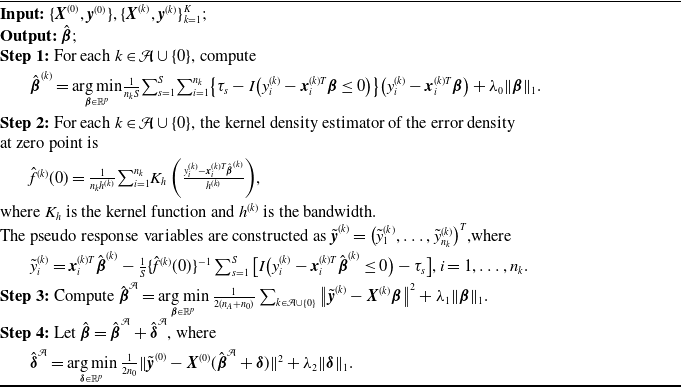
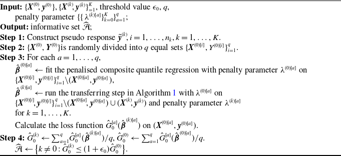
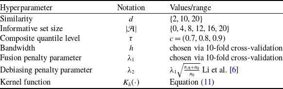

 d

 d

 d

 d

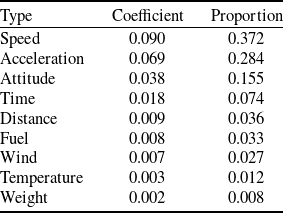
 τ=c(0.85,0.9,0.95)

 τ=c(0.85,0.9,0.95)
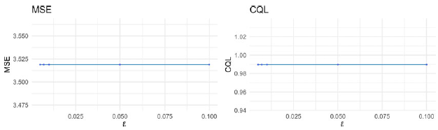
 ϵ0
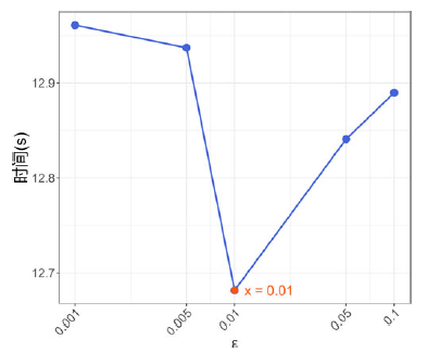
 ϵ0