





1. Introduction and the main result
We fix a time horizon
 $T\lt\infty$
and consider a financial market that consists of a safe asset earning zero interest rate and of a risky asset
 $S_t$
,
 $t\in [0,T]$
that follows the Ornstein–Uhlenbeck diffusion process
 \begin{equation}{\mathrm{d}} S_t=(\mu-S_t) \,{\mathrm{d}} t+{\mathrm{d}} W_t,\end{equation}
where
 $\mu\in\mathbb R$
is the long-term mean and
 $W_t$
,
 $t\geq 0$
is a standard one-dimensional Brownian motion defined on a probability space
 $(\Omega,\mathcal F,\mathbb P)$
and endowed with the augmented natural filtration
 $\mathcal F_t$
,
 $t\geq 0$
. As usual, we assume that the initial stock price is a given constant
 $S_0$
. Without loss of generality we assume that
 $\mathcal F=\mathcal F_T$
.
Our motivation to study optimal investments with a mean reverting risky asset comes from the recent paper by Guasoni et al. [Reference Guasoni, Nagy and Rásonyi10], who considered asymptotically (as the time horizon goes to infinity) optimal investments for mean reverting risky assets. Although they considered a more general type of mean reverting models than the linear Ornstein–Uhlenbeck diffusion, they assumed that the trading is frictionless.
In financial markets, trading moves prices against the trader: buying faster increases execution prices, and selling faster decreases them. This aspect of liquidity, known as market depth [Reference Black5] or price impact, has recently received increasing attention; see e.g. [Reference Alfonsi, Fruth and Schied1], [Reference Bayraktar, Caye and Ekren4], [Reference Caye, Herdegen and Muhle-Karbe6], [Reference Fruth, Schöneborn and Urusov9], [Reference Moreau, Muhle-Karbe and Soner13], [Reference Nadtochiy14], and the references therein.
Following [Reference Almgren and Chriss2], we model this impact in a temporary linear form and, thus, when at time t the investor turns over her position
 $\Phi_t$
at the rate
 $\phi_t=\dot{\Phi}_t$
, the execution price is
 $S_t+{{\phi_t}/{(2\delta)}}$
for some constant
 $\delta\gt0$
that denotes the market depth. As a result, the profits and losses from trading are given by
 \begin{equation}V^{\Phi_0,\phi}_T\, :\!= \, \Phi_0(S_T-S_0)+\int_{0}^T \phi_t(S_T-S_t)\,{\mathrm{d}} t-\dfrac{1}{2\delta} \int_{0}^T \phi^2_t \,{\mathrm{d}} t,\end{equation}
where, for convenience, we assume that the investor marks to market her position
 $\Phi_T = \Phi_0+\int_0^T \phi_t \,{\mathrm{d}} t$
in the risky asset that she has acquired by time
 $T\gt0$
.
The natural class of admissible strategies is given by
 \begin{align*}\mathcal A\, :\!= \, \biggl\{\phi=(\phi_t)_{t\in [0,T]}\colon \ \phi \text{ is } \ \mathcal F_t\text{-optional with } \int_{0}^T \phi^2_t \,{\mathrm{d}} t\lt\infty \ \text{ a.s.}\biggr\}.\end{align*}
Let us explain formula (1.2) in more detail. At time 0, the investor holds
 $\Phi_0$
shares of the stock and an amount
 $-\Phi_0 S_0$
in the savings account. At time
 $t \in [0,T]$
, the investor purchases
 $\phi_t\,{\mathrm{d}} t$
, an infinitesimal number of shares. Consequently, the (infinitesimal) change in the savings account is
 \begin{align*}-\phi_t\biggl(S_t+\dfrac{\phi_t}{2\delta}\biggr)\,{\mathrm{d}} t . \end{align*}
The terminal portfolio value consists of the terminal balance in the savings account together with the value of the stock holdings. Hence it is given by
 \begin{align*}-\Phi_0 S_0-\int_0^T \phi_t\biggl(S_t+\dfrac{\phi_t}{2\delta}\biggr)\,{\mathrm{d}} t+\Phi_T S_T. \end{align*}
Since
 $\Phi_T=\Phi_0+\int_{0}^T \phi_t\,{\mathrm{d}} t,$
we obtain the right-hand side of (1.2).
The investor’s preferences are described by an exponential utility function
 $u(x)=-\exp$
 $({-}\alpha x)$
,
 $x\in\mathbb R$
, with absolute risk aversion parameter
 $\alpha\gt0$
, and her goal is to
 \begin{align}\text{maximize}\ \mathbb E_{\mathbb P}\bigl[u\bigl(V^{\Phi_0,\phi}_T\bigr)\bigr]=\mathbb E_{\mathbb P}\bigl[-\exp\bigl({-}\alpha V^{\Phi_0,\phi}_T\bigr)\bigr]\text{ over } {\phi\in\mathcal A},\end{align}
where
 $\mathbb E_{\mathbb P}$
denotes the expectation with respect to the underlying probability measure
 $\mathbb P$
. Observe that for any
 $(\Phi_0,\phi)\in \mathbb{R}\times\mathcal{A}$
, we have
 $\alpha V_T^{\Phi_0,\phi}=\tilde V_T^{\alpha\Phi_0,\alpha\phi},$
where
 $\tilde V^{\cdot}_{\cdot}$
is defined by (1.2) with market depth
 $\tilde\delta\, :\!= \, \alpha\delta$
. Thus, without loss of generality, we take
 $\alpha=1$
.
The paper’s main result is the following solution to the optimization problem (1.3). For simplicity we assume that the initial number of shares is
 $\Phi_0=0$
.
Theorem 1.1. Set
 \begin{align*}\mathcal V(t)\, :\!= \, \dfrac{\sqrt{ 1+\delta} ({\sinh}(\sqrt{1+\delta} t ) + \sqrt{1+\delta} (1+\delta+\delta t) \cosh(\sqrt{1+\delta}t))}{\sqrt{1+\delta} (1+\delta+\delta t) \sinh(\sqrt{1+\delta} \, t) + (1+\delta^2) \cosh(\sqrt{1+\delta}t) + 2{\delta}}-1, \quad t\geq 0. \end{align*}
The utility maximization problem (1.3) has a unique optimal hedging strategy
 $\hat \phi_t$
,
 $t\in [0,T]$
which is given by the feedback form
 \begin{equation}\hat\phi_t=\delta\dfrac{\bigl(1+\frac{1-\delta}{(1+\delta)^{3/2}}\tanh\bigl(\frac{\sqrt{1+\delta}(T-t)}{2}\bigr)+\frac {\delta (T-t) }{1+\delta}\bigr)(\mu-S_t)-\hat\Phi_t}{1+\frac {\delta (T-t) }{1+\delta}+\frac{\sqrt{1+\delta}}{\sinh(\sqrt{1+\delta} (T-t))}+\frac{1+\delta^2}{(1+\delta)^{3/2}}\tanh\bigl(\frac{\sqrt{1+\delta}(T-t)}{2}\bigr)},\end{equation}
where
 \begin{align*}\hat\Phi_t\, :\!= \, \int_{0}^t\hat\phi_s \,{\mathrm{d}} s,\quad t\in [0,T]. \end{align*}
The corresponding value is equal to
 \begin{equation}\mathbb E_{\mathbb P}\bigl[-\exp\bigl({-} V^{0,\hat\phi}_T\bigr)\bigr]=-\exp\biggl({-}\dfrac{1}{2}\mathcal V(T)(\mu-S_0)^2-\dfrac{1}{2}\int_{0}^T \mathcal V(t)\,{\mathrm{d}} t\biggr). \end{equation}
Let us collect some financial-economic observations from this result. First, direct calculations yield that the derivative of
 $\mathcal V$
is equal to
 \begin{align*}\dot{\mathcal V}(t)=\dfrac{\delta(1+\delta)(A(t)+B(t)+\delta^2\sinh^2(\sqrt{1+\delta}t)) }{(\sqrt{1+\delta} (1+\delta+\delta t) \sinh(\sqrt{1+\delta}t) + (1+\delta^2) \cosh(\sqrt{1+\delta}t) + 2{\delta})^{2}},\end{align*}
where
 \begin{align*}&A(t)\, :\!= \, 2(1+\delta+\delta t)\sqrt{1+\delta}\sinh(\sqrt{1+\delta}t)-2(1+\delta)^2 t , \\[3pt] &B(t)\, :\!= \, 2(1+\delta)\cosh(\sqrt{1+\delta}t)-2(1+\delta)-(\delta+\delta^2) t^2.\end{align*}
Clearly,
 $\sinh(\sqrt{1+\delta}t)\geq\sqrt{1+\delta}t$
and
 $\cosh(\sqrt{1+\delta}t)\geq 1+{{(1+\delta)}/{2}} t^2$
for all t. Thus
 $A,B\geq 0$
. We conclude that
 $\dot{\mathcal V}(t)\gt0$
for
 $t\gt0$
. Since
 $\mathcal V(0)=0$
, we get
 $\mathcal V(t)\gt0$
for
 $t\gt0$
. Hence, from (1.5) the optimal expected utility is increasing in the following two parameters: (i) the time horizon T, and (ii) the term
 $|\mu-S_0|$
, namely the distance between the initial stock price and the long-term mean of the Ornstein–Uhlenbeck diffusion process.
Obviously, for
 $(\Phi_0,\phi)\in \mathbb{R}\times\mathcal{A}$
, the corresponding portfolio is increasing in the market depth
 $\delta$
. Consequently, the value of the optimization problem (1.3) is increasing in the market depth
 $\delta$
. As
 $\delta \downarrow 0$
, we have
 $\mathcal{V}(t) \downarrow 0$
, and hence the corresponding expected utility converges to
 $-1$
. This is intuitively clear: as the market depth approaches zero, any non-zero trading strategy incurs an infinite penalty, making the zero strategy optimal.
On the other hand, as the market depth tends to infinity, the function
 $\mathcal{V}(t)$
converges to t. Consequently, the value converges to
 $-\exp\bigl({-\frac{1}{2}T|\mu - S_0|^2 - \frac{1}{2}T^2}\bigr),$
which coincides with the value of the frictionless utility maximization problem (see Section 3 in [Reference Guasoni, Nagy and Rásonyi10]).
Next, for a fixed
 $\delta\gt0$
, we have
 $\lim_{t\rightarrow\infty} \mathcal V(t)=\sqrt{1+\delta}-1$
. Thus the certainty equivalent
 \begin{align*}c(T)\, :\!= \, -\log\bigl(\mathbb E_{\mathbb P}\bigl[\exp\bigl({-} V^{0,\hat\phi}_T\bigr)\bigr]\bigr) \end{align*}
(the optimal strategy
 $\hat\phi$
depends on the time horizon T) satisfies
 \begin{equation}\lim_{T\rightarrow\infty} \dfrac{c(T)}{T}=\dfrac{\sqrt{1+\delta}-1}{2}.\end{equation}
Let us notice that for the frictionless case (see Section 3 in [Reference Guasoni, Nagy and Rásonyi10]), the certainty equivalent is of order
 $T^2$
(for large T).
The feedback description (1.4) says that the optimal trading strategy is a mean reverting strategy towards the process
 \begin{equation*}X_t\, :\!= \, \biggl(1+\dfrac{1-\delta}{(1+\delta)^{3/2}}\tanh\biggl(\dfrac{\sqrt{1+\delta}(T-t)}{2}\biggr)+\dfrac {\delta (T-t) }{1+\delta}\biggr)(\mu-S_t), \quad t\in [0,T].\end{equation*}
This process depends linearly on the difference between the long-term mean
 $\mu$
and the current stock price
 $S_t$
. If the current time t is close to the maturity date T, the value of
 $X_t$
is close
 $\mu-S_t$
. If
 $T-t$
is large then
 $X_t$
is of order
 ${{(\delta(T-t))}/{(1+\delta)}}(\mu-S_t)$
. The denominator in (1.4) describes how fast (as a function of time) the investor should trade towards the process X. Notice that the denominator is large if the time left until the maturity date
 $T-t$
is large or small. Namely, in both of these cases the investor should trade slowly towards the process X.
For the case where the market depth goes to infinity, i.e.
 $\delta\rightarrow\infty$
, the process X converges (almost surely) to
 $(1+T-t)(\mu-S_t)$
,
 $t\in [0,T]$
. Observe that the denominator in (1.4) is of order
 $\sqrt \delta$
(for large
 $\delta$
) and so, for the case where the friction vanishes, the optimal number of shares
 $\hat\Phi_t$
converges to
 $(1+T-t)(\mu-S_t)$
, which is exactly the optimal strategy for the frictionless utility maximization problem (see Section 3 in [Reference Guasoni, Nagy and Rásonyi10]).
We end this section with the following two remarks.
Remark 1.1. For a simplified presentation and economy of notation, we assume that the mean-reversion rate and the volatility of the Ornstein–Uhlenbeck diffusion process are normalized to 1. Observe that for given
 $\kappa,\sigma\gt0$
, the process
 $Y_t \, :\!= \, ({{\sigma}/{\sqrt{\kappa}}}) S_{\kappa t}$
,
 $t\geq 0$
satisfies the SDE
 \begin{align*}{\mathrm{d}} Y_t = \kappa\biggl(\dfrac{\sigma \mu}{\sqrt{\kappa}} - Y_t\biggr) \,{\mathrm{d}} t + \sigma {\mathrm{d}}\hat W_t,\quad Y_0 = \dfrac{\sigma S_0}{\sqrt{\kappa}}, \end{align*}
where
 $\hat W$
is a standard Brownian motion defined by
 $\hat W_t \, :\!= \, ({{1}/{\sqrt{\kappa}}}) W_{\kappa t}$
,
 $t\geq 0$
. Moreover, for any
 $(\Phi_0,\phi)\in \mathbb{R}\times\mathcal{A}$
we have
 \begin{align*}V^{\Phi_0,\phi}_T=\hat\Phi_0(Y_{\hat T} - Y_0)+ \int_{0}^{\hat T} \hat\phi_{t} (Y_{\hat T} - Y_t)\, {\mathrm{d}} t- \dfrac{1}{2\hat\delta} \int_{0}^{\hat T} \hat\phi_t^2 \, {\mathrm{d}} t, \end{align*}
where
 \begin{align*}\hat{\Phi}_0 \, :\!= \, \frac{\Phi_0 \sqrt{\kappa}}{\sigma},\quad \hat T \, :\!= \, \frac{T}{\kappa},\quad \hat\delta \, :\!= \, \frac{\kappa^2\delta}{\sigma^2}\quad \text{and}\quad \hat\phi_t \, :\!= \, \frac{\kappa^{3/2}}{\sigma}\phi_{\kappa t},\quad t\in [0,\hat T]. \end{align*}
Thus, in the case where the initial number of shares is
 $\Phi_0 = 0$
, the value of the exponential utility maximization problem with maturity date
 $\hat T \gt 0$
, initial stock price
 $\hat S_0$
, long-term mean
 $\hat\mu$
, mean-reversion
 $\kappa \gt 0$
, volatility
 $\sigma \gt 0$
, and market depth
 $\hat\delta \gt 0$
, is equal to the value of (1.3) with the rescaled parameters of maturity date
 $\kappa \hat T$
, initial stock price
 $({{\sqrt{\kappa}}/{\sigma}})\hat S_0$
, long-term mean
 $({{\sqrt{\kappa}}/{\sigma}})\hat\mu$
, and market depth
 $({{\sigma^2}/{\kappa^2}})\hat\delta$
.
From (1.6) and the above analysis, we obtain that the corresponding certainty equivalent satisfies
 \begin{align*}\lim_{T \to \infty} \frac{c(T)}{T}= \frac{\sqrt{1 + {{\sigma^2 \hat\delta}/{\kappa^2}}} - 1}{2}. \end{align*}
Observe that this expression is decreasing in the mean-reversion parameter
 $\kappa \gt 0$
and increasing in the volatility
 $\sigma \gt 0$
.
On the other hand, suppose that the maturity date is fixed and the market depth goes to infinity. Then, from the discussion following Theorem 1.1, we conclude that the corresponding value converges (as
 $\hat\delta \to \infty$
) to
 \begin{align*}{- \exp\biggl({-\frac{\kappa^2}{\sigma^2} T |\hat\mu - \hat S_0|^2 - \frac{1}{2}\kappa^2 \hat T^2}\biggr).} \end{align*}
This expression is clearly increasing in
 $\kappa$
and decreasing in
 $\sigma$
. Thus there is no uniform pattern regarding monotonicity with respect to the mean-reversion and volatility parameters.
Remark 1.2. The proof of Theorem 1.1 relies on the duality result for exponential hedging with quadratic transaction costs given in Proposition A.2 of [Reference Bank, Dolinsky and Rásonyi3]. From a financial perspective, one limitation of our setup is that we do not impose liquidation of the position at the maturity date, that is, we do not include the constraint
 $\Phi_T = 0$
.
A duality result for the case with a liquidation constraint is also available (see [Reference Dolinsky7]). In particular, Theorem 2.1 in [Reference Dolinsky7] extends Proposition A.2 of [Reference Bank, Dolinsky and Rásonyi3] to the setting where liquidation at maturity is required. The liquidation constraint introduces additional difficulties in the dual representation. Specifically, the maximization is taken over all equivalent probability measures together with the corresponding martingales, whereas in Proposition A.2 of [Reference Bank, Dolinsky and Rásonyi3] the dual variables consist only of equivalent probability measures (compare (2.3)–(2.4) in [Reference Dolinsky7] with (2.2)–(2.3) in the current paper).
This additional structure makes the resulting computations substantially more involved. In [Reference Dolinsky7], for example, we considered the problem of hedging a quadratic option in the Bachelier model. Even in this relatively simple setting, the computations arising from the dual formulation are quite complicated (see Proposition 4.1 in [Reference Dolinsky7]). In fact, we were only able to determine the optimal portfolio, but not the corresponding value of the optimization problem.
For these reasons, we do not impose a liquidation constraint in the present paper. Moreover, even in the current setting without a liquidation constraint, in order to express the value of the optimization problem (1.3) in a tractable form, we assume that the initial number of shares satisfies
 $\Phi_0 = 0$
. This assumption simplifies the computations in Lemma 3.2.
2. Proof of Theorem 1.1
Our proof will be based on a change of measure and the duality result given by Proposition A.2 in [Reference Bank, Dolinsky and Rásonyi3].
Set
 $B_t \, :\!= \, S_t - S_0$
,
 $t \ge 0$
. From (1.1),
 \begin{align*}B_t=(S_0 - \mu) ({\mathrm{e}}^{-t}-1)+\int_0^t {\mathrm{e}}^{-(t-s)}\, {\mathrm{d}} W_s, \quad t\geq 0. \end{align*}
Namely,
 $B_t$
,
 $t\in [0,T]$
, is of the form
 \begin{align*}B_t=\gamma_t+\int_{0}^t m_{t,s} \, {\mathrm{d}} W_s, \end{align*}
for
 $\gamma\in L^2[0,T]$
and a Volterra kernel
 $m\in L^2([0,T]^2)$
. Since
 ${\mathrm{d}} B_t = {\mathrm{d}} W_t + (\mu - S_0 - B_t)\,{\mathrm{d}} t$
,
 $t\geq 0$
, then from Theorem 2′ in [Reference Hitsuda11] it follows that there exists a probability measure
 $\hat{\mathbb P}\sim\mathbb P$
such that
 $B_t$
,
 $t\in [0,T]$
is a Brownian motion with respect to
 $\hat{\mathbb P}$
. Clearly,
 ${\mathrm{d}} W_t = {\mathrm{d}} B_t - (\mu - S_0 - B_t)\,{\mathrm{d}} t$
,
 $t\geq 0$
. Thus, by applying Theorem 2′ in [Reference Hitsuda11] again, we obtain that the corresponding Radon–Nikodým derivative is given by
 ${{{\mathrm{d}}\mathbb P}/{{\mathrm{d}}\hat{\mathbb P}}} = {\mathrm{e}}^X$
, where
 \begin{align}X&\, :\!= \, \int_{0}^T (\mu - S_0 - B_t)\,{\mathrm{d}} B_t - \frac{1}{2}\int_{0}^T (\mu - S_0 - B_t)^2\, {\mathrm{d}} t \nonumber\\[3pt] &= \frac{T}{2} + (\mu - S_0)B_T - \frac{B_T^2}{2} - \frac{1}{2}\int_{0}^T (\mu - S_0 - B_t)^2\, {\mathrm{d}} t .\end{align}
Next, we apply Proposition A.2 in [Reference Bank, Dolinsky and Rásonyi3]. We begin by verifying the integrability condition in Assumption A.1 of [Reference Bank, Dolinsky and Rásonyi3]. Since
 $B_t$
,
 $t\in [0,T]$
is a Brownian motion with respect to
 $\hat{\mathbb P}$
, there exists a constant
 $c\gt0$
such that
 \begin{align*}\mathbb E_{\hat{\mathbb P}}\Bigl[\exp\Bigl(c\max_{0\le t\le T} B_t^2\Bigr)\Bigr] \lt \infty . \end{align*}
This, together with the Cauchy–Schwarz inequality, (2.1), and the elementary bound
 \begin{align*}S_t^2 \le 2\bigl(S_0^2 + B_t^2\bigr),\quad t\geq 0 , \end{align*}
gives
 \begin{align*}\mathbb{E}_{\mathbb{P}}\biggl[\exp\biggl(\dfrac{c}{4}\max_{0\le t\le T} S_t^2\biggr)\biggr]\le\mathbb{E}_{\hat{\mathbb{P}}}\biggl[\exp\biggl(\dfrac{cS_0^2+T}{2}+(\mu-S_0)B_T+\dfrac{c}{2}\max_{0\le t\le T} B_t^2\biggr)\biggr]\lt\infty . \end{align*}
Hence Assumption A.1 in [Reference Bank, Dolinsky and Rásonyi3] holds.
Clearly, for any probability measure
 $\mathbb Q\sim\mathbb P$
we have
 \begin{align*}\log\biggl(\frac{{\mathrm{d}}\mathbb Q}{{\mathrm{d}}{\mathbb P}}\biggr)=\log\biggl(\frac{{\mathrm{d}}\mathbb Q}{{\mathrm{d}}\hat{\mathbb P}}\biggr)-X. \end{align*}
Thus, from Proposition A.2 in [Reference Bank, Dolinsky and Rásonyi3], we obtain the following duality:
 \begin{align}&\max_{\phi\in\mathcal A}\bigl\{-\log\bigl(\mathbb E_{\mathbb P}\bigl[\exp\bigl({-}V^{\Phi_0,\phi}_T\bigr)\bigr]\bigr)\bigr\}\nonumber\\[3pt] &\quad =\inf_{\mathbb Q\in \mathcal Q}\mathbb E_{\mathbb Q}\biggl[\Phi_0 B_T-X+\log\biggl(\dfrac{{\mathrm{d}}\mathbb Q}{{\mathrm{d}}\hat{\mathbb P}}\biggr)+\dfrac{\delta}{2}\int_{0}^T(\mathbb E_{\mathbb Q}[B_T-B_t|\mathcal F_t])^2 \,{\mathrm{d}} t\biggr],\end{align}
where
 $\mathcal Q$
is the set of all probability measures
 $\mathbb Q\sim \hat{\mathbb P}$
with finite relative entropy
 \begin{align*}\mathbb E_{\mathbb Q}\biggl[{\log}\frac{{\mathrm{d}}\mathbb Q}{{\mathrm{d}}\hat{\mathbb P}} \biggr]\lt\infty. \end{align*}
The same proposition also yields that there exists a unique solution
 $\hat{\mathbb Q}$
to the dual problem, and it allows us to construct the unique solution
 $\hat{\phi}$
to the primal problem as
 \begin{equation} \hat{\phi}_t = \delta \mathbb E_{\hat{\mathbb Q}}[B_T-B_t|\mathcal F_t], \quad t \in [0,T].\end{equation}
We arrive at the following lemma.
Lemma 2.1. The dual infimum in (2.2) coincides with the one taken over all
 $\mathbb Q \in \mathcal Q$
, whose densities take the form
 \begin{equation}\dfrac{{\mathrm{d}}\mathbb Q}{{\mathrm{d}}\hat{\mathbb P}} = \exp\biggl(\int_0^T \eta_t \,{\mathrm{d}} B_t-\dfrac{1}{2}\int_0^T\eta_t^2\,{\mathrm{d}} t\biggr) \end{equation}
for some bounded and adapted
 $\eta$
changing values only at finitely many deterministic times. For such
 $\mathbb Q$
, the induced value for the dual problem can be written as
 \begin{align}&\mathbb E_{\mathbb Q}\biggl[\Phi_0 B_T-X+\log\biggl(\dfrac{{\mathrm{d}}\mathbb Q}{{\mathrm{d}}\hat{\mathbb P}}\biggr)+\dfrac{\delta}{2}\int_{0}^T(\mathbb E_{\mathbb Q}[B_T-B_t|\mathcal F_t])^2 \,{\mathrm{d}} t\biggr]\nonumber\\[3pt] &\quad =-\dfrac{T}{2}+(\Phi_0-(\mu-S_0))\int_{0}^T a_t \,{\mathrm{d}} t+\dfrac{1}{2}\biggl(\int_{0}^T a_t \,{\mathrm{d}} t\biggr)^2+\dfrac{1}{2}\int_{0}^T a^2_t \,{\mathrm{d}} t \notag\\[3pt] &\quad \quad +\dfrac{1}{2}\int_{0}^T\biggl(\int_{0}^t a_s \,{\mathrm{d}} s-(\mu-S_0)\biggr)^2 \,{\mathrm{d}} t+\dfrac{\delta}{2}\int_{0}^T \biggl(\int_{t}^T a_s \,{\mathrm{d}} s\biggr)^2 \,{\mathrm{d}} t\nonumber\\[3pt] &\quad \quad +\int_{0}^T \mathbb E_{\mathbb Q}\biggl[\dfrac{1}{2}\biggl(1+\int_{s}^T l_{t,s} \,{\mathrm{d}} t\biggr)^2+\dfrac{1}{2}\int_{s}^T\biggl(1+\int_{s}^t l_{u,s}\,{\mathrm{d}} u\biggr)^2 \,{\mathrm{d}} t \nonumber\\[3pt] &\quad \quad +\dfrac{1}{2}\int_{s}^T l^2_{t,s}\,{\mathrm{d}} t+\dfrac{\delta}{2}\int_{s}^T \biggl(\int_{t}^T l_{u,s} \,{\mathrm{d}} u\biggr)^2 \,{\mathrm{d}} t\biggr]\,{\mathrm{d}} s ,\end{align}
where, for
 $t\in[0,T]$
,
 $a_t$
and
 $l_{t,.}=(l_{t,s})_{s\in [0,t]}$
such that
 $\mathbb E_{\mathbb Q}\bigl[\int_{0}^t l^2_{t,s}\,{\mathrm{d}} s\bigr]\lt\infty$
are determined by the Itô representations
 \begin{equation} \eta_t = a_t + \int_0^t l_{t,s} \,{\mathrm{d}} W^{\mathbb Q}_s , \end{equation}
with respect to the
 $\mathbb Q$
-Brownian motion
 $W^{\mathbb Q}_s=B_s-\int_0^s \eta_r \,{\mathrm{d}} r$
,
 $s\in [0,T]$
.
Proof. For any
 $\mathbb Q \in \mathcal Q$
the martingale representation property of Brownian motion gives us a predictable
 $\eta$
with
 \begin{align*}\mathbb E_{\mathbb Q}[{\log}({\mathrm{d}}\mathbb Q/{\mathrm{d}}\hat{\mathbb P})]=\mathbb E_{\mathbb Q}\biggl[\int_0^T\eta^2_s\,{\mathrm{d}} s\biggr]/2 \lt \infty \\[-20pt] \end{align*}
such that the density
 ${\mathrm{d}}\mathbb Q/{\mathrm{d}}\hat{\mathbb P}$
takes the form (2.4). Using this density to rewrite the dual target functional as an expectation under
 $\hat{\mathbb P}$
, we can follow standard density arguments in
 $L^2({\mathrm{d}} t\otimes\hat{\mathbb P})$
(see Section 3.2 in [Reference Karatzas and Shreve12]) to see that the infimum over
 $\mathbb Q \in \mathcal Q$
can be realized by considering the
 $\mathbb Q$
induced via (2.4) by simple
 $\eta$
as described in the lemma’s formulation. As a consequence, the Itô representations of
 $\eta_t$
in (2.6) can be chosen in such a way that the resulting
 $(a_t,l_{t,.})$
are also measurable in t: in fact they only change when
 $\eta$
changes its value, i.e. at finitely many deterministic times. This joint measurability will allow us below to apply Fubini’s theorem freely. Let us rewrite the dual target functional, given in terms of a and l, in terms of
 $\eta$
and the
 $\mathbb Q$
-Brownian motion
 $W^{\mathbb Q}$
.
First, from Itô’s isometry and Fubini’s theorem, we obtain
 \begin{equation}\mathbb E_{\mathbb Q}\biggl[\int_{0}^T \eta^2_u \,{\mathrm{d}} u\biggr] =\int_{0}^T a^2_t \,{\mathrm{d}} t+\int_{0}^T\int_{s}^{T}\mathbb E_{\mathbb Q}\bigl[l^2_{t,s} \bigr]\,{\mathrm{d}} t\, {\mathrm{d}} s.\end{equation}
Again by Fubini’s theorem it follows that
 \begin{align*}\mathbb E_{\mathbb Q}\biggl[\int_{t}^T \eta_u\,{\mathrm{d}} u \biggm|\mathcal F_t\biggr] & =\int_{t}^T a_u \,{\mathrm{d}} u+\mathbb E_{\mathbb Q}\biggl[\int_{0}^T\int_{t}^T l_{u,s}\,{\mathrm{d}} u\, {\mathrm{d}} W^{\mathbb Q}_s\biggm|\mathcal F_t\biggr]\\[3pt] &=\int_{t}^T a_u \,{\mathrm{d}} u+\int_{0}^{t} \int_{t}^T l_{u,s} \,{\mathrm{d}} u\, {\mathrm{d}} W^{\mathbb Q}_s, \quad t\in [0,T],\end{align*}
where the last equality follows from the martingale property of stochastic integrals. Thus another application of Itô’s isometry and Fubini’s theorem yields
 \begin{align*} \int_{0}^T(\mathbb E_{\mathbb Q}[B_T-B_t|\mathcal F_t])^2 \,{\mathrm{d}} t & =\int_{0}^T\biggl(\mathbb E_{\mathbb Q}\biggl[\int_{t}^T \eta_u\,{\mathrm{d}} u \biggm|\mathcal F_t\biggr]\biggr)^2 \,{\mathrm{d}} t\nonumber\\[3pt] &=\int_{0}^T\biggl(\int_{t}^T a_u \,{\mathrm{d}} u\biggr)^2 \,{\mathrm{d}} t+\int_{0}^T\mathbb E_{\mathbb Q}\biggl[\int_{s}^T \biggl(\int_{t}^T l_{u,s} \,{\mathrm{d}} u\biggr)^2 \,{\mathrm{d}} t\biggr]\,{\mathrm{d}} s.\end{align*}
By applying again Itô’s isometry and Fubini’s theorem, we obtain
 \begin{equation*} \mathbb E_{\mathbb Q}\bigl[B^2_T\bigr]=\biggl(\int_{0}^T a_t \,{\mathrm{d}} t\biggr)^2+\int_{0}^T\mathbb E_{\mathbb Q}\biggl[\biggl(1+\int_{s}^T l_{u,s} \,{\mathrm{d}} u\biggr)^2\biggr] \,{\mathrm{d}} s\end{equation*}
and
 \begin{align}&\mathbb E_{\mathbb Q}\biggl[\int_{0}^T (B_t-(\mu-S_0))^2 \,{\mathrm{d}} t\biggr]\nonumber\\[3pt] &\quad =\int_{0}^T\biggl(\int_{0}^t a_s \,{\mathrm{d}} s-(\mu-S_0)\biggr)^2 \,{\mathrm{d}} t+\int_{0}^T \mathbb E_{\mathbb Q}\biggl[\int_{s}^T\biggl(1+\int_{s}^t l_{u,s} \,{\mathrm{d}} u\biggr)^2\,{\mathrm{d}} t\biggr]\,{\mathrm{d}} s.\end{align}
Plugging (2.1) and (2.7)–(2.8) into the left-hand side of (2.5) provides us with the claimed formula.
We now have all the pieces in place that we need to complete the proof of Theorem 1.1.
Proof. The crucial point of the above representation is that by taking the minimum separately over a and over
 $l_{.,s}$
for each
 $s \in [0,T]$
, we obtain deterministic variational problems that can be solved explicitly, and this deterministic minimum yields the solution to the dual problem. Namely, from Lemma 3.2 it follows that there exists deterministic functions
 $\hat a, \hat{\kern-1.3pt l}$
which minimize the right-hand side of (2.5). Theorem 2 in [Reference Hitsuda11] yields a probability measure
 $\hat{\mathbb Q}$
that satisfies
 \begin{align*}\dfrac{{\mathrm{d}}\hat{\mathbb Q}}{{\mathrm{d}}\hat{\mathbb P}} = \exp\biggl(\int_0^T \hat\eta_t \,{\mathrm{d}} B_t-\dfrac{1}{2}\int_0^T\hat\eta_t^2\,{\mathrm{d}} t\biggr) \end{align*}
for
 \begin{align*}\hat\eta_t = \hat a_t + \int_0^t \hat{\kern-1.3pt l}_{t,s} \,{\mathrm{d}} W^{\hat{\mathbb Q}}_s,\quad t\in [0,T]. \end{align*}
The probability measure
 $\hat{\mathbb Q}$
is the unique solution to the dual problem given by the right-hand side of (2.2).
From (2.3) and (3.2) (
 $\hat h=\hat a$
,
 $s=0$
), we obtain
 \begin{align*} \hat\phi_0=\delta\int_{0}^T \hat a_t \,{\mathrm{d}} t=\frac{\bigl(1+\frac{1-\delta}{(1+\delta)^{3/2}}\tanh\bigl(\frac{\sqrt{1+\delta} T}{2}\bigr)+\frac {\delta T }{1+\delta}\bigr)(\mu-S_t)-\Phi_0}{1+\frac {\delta T }{1+\delta}+\frac{\sqrt{1+\delta}}{\sinh(\sqrt{1+\delta}T)}+\frac{1+\delta^2}{(1+\delta)^{3/2}}\tanh\bigl(\frac{\sqrt{1+\delta} T}{2}\bigr)}. \end{align*}
This gives (1.4) for
 $t=0$
. We claim that (1.4) holds for every
 $t \in [0,T]$
. To this end, we apply the dynamic programming argument used in Lemma 3.5 of [Reference Bank, Dolinsky and Rásonyi3]. Assume by contradiction that the statement fails. By (2.3), the sample paths of the unique optimal portfolio
 $\hat{\phi}$
are continuous. Hence there exists
 $t_0 \in [0,T]$
such that, with positive probability,
 $\hat{\phi}_{t_0}$
does not coincide with the right-hand side of (1.4). Now consider the strategy
 $\tilde{\phi}$
which coincides with
 $\hat{\phi}$
up to time
 $t_0$
and is given by (1.4) for
 $t\geq t_0$
. For any strategy
 $\phi$
, we can write the contribution over the interval
 $[t_0,T]$
to the resulting terminal wealth as
 \begin{align*}V_T^{\Phi_0,\phi} - V_{t_0}^{\Phi_0,\phi}= {\Phi}_{t_0}(S_T-S_{t_0})+ \int_{t_0}^T \phi_t(S_T-S_t)\,{\mathrm{d}} t- \dfrac{1}{2\delta}\int_{t_0}^T \phi_t^2\,{\mathrm{d}} t\,=\!:\, V^{\Phi_{t_0},\phi}_{[t_0,T]}, \end{align*}
where
 $V_{t_0}^{\Phi_0,\phi}$
denotes the portfolio value at time
 $t_0$
, defined by (1.2) with T replaced by
 $t_0$
. Thus, by the Markov property of
 $S_t$
,
 $t\in[0,T]$
, and by the choice of
 $\tilde{\phi}$
as the unique optimal policy from time
 $t_0$
onward, we obtain
 \begin{align*}\mathbb{E}_{\mathbb{P}}\Bigl[-\exp\Bigl({-} V^{\tilde\Phi_{t_0},\tilde\phi}_{[t_0,T]}\Bigr)\mid \mathcal F_{t_0}\Bigr]\ge\mathbb{E}_{\mathbb{P}}\Bigl[-\exp\Bigl({-}V^{\hat\Phi_{t_0},\hat\phi}_{[t_0,T]}\Bigr)\mid \mathcal F_{t_0}\Bigr], \end{align*}
with strict inequality on
 $\{\hat\phi_{t_0}\neq \tilde\phi_{t_0}\}$
(i.e. where (1.4) is violated), since the continuity of
 $\hat\phi$
and
 $\tilde\phi$
implies that once they differ at
 $t_0$
, they must differ on an open interval.
Since, by assumption, this occurs with positive probability, it follows for the unconditional expected utility of
 $\tilde\phi$
that
 \begin{align*}\mathbb{E}_{\mathbb{P}}\Bigl[-\exp\Bigl({-}V_T^{\Phi_0,\tilde\phi}\Bigr)\Bigr]&=\mathbb{E}_{\mathbb{P}}\Bigl[\exp\Bigl({-}V_{t_0}^{\Phi_0,\tilde\phi}\Bigr)\mathbb{E}_{\mathbb{P}}\Bigl[-\exp\Bigl({-}V^{\tilde\Phi_{t_0},\tilde\phi}_{[t_0,T]}\Bigr)\mid \mathcal F_{t_0}\Bigr]\Bigr]\\[3pt] &\gt\mathbb{E}_{\mathbb{P}}\Bigl[\exp\Bigl({-} V_{t_0}^{\Phi_0,\tilde\phi}\Bigr)\mathbb{E}_{\mathbb{P}}\Bigl[-\exp\Bigl({-}V^{\hat\Phi_{t_0},\hat\phi}_{[t_0,T]}\Bigr)\mid\mathcal F_{t_0}\Bigr]\Bigr]\\[3pt] &=\mathbb{E}_{\mathbb{P}}\Bigl[-\exp\Bigl({-} V_T^{\Phi_0,\hat\phi}\Bigr)\Bigr],\end{align*}
contradicting the optimality of
 $\hat\phi$
.
Next, we establish (1.5). By applying (3.3) for
 $\theta\, :\!= \, -1$
, we get
 \begin{align*}&\dfrac{1}{2}\biggl(1+\int_{s}^T \hat{\kern-1.3pt l}_{t,s} \,{\mathrm{d}} t\biggr)^2+\dfrac{1}{2}\int_{s}^T\biggl(1+\int_{s}^t \hat{\kern-1.3pt l}_{u,s}\,{\mathrm{d}} u\biggr)^2 \,{\mathrm{d}} t\\[3pt] &\quad +\dfrac{1}{2}\int_{s}^T \hat{\kern-1.3pt l}^2_{t,s}\,{\mathrm{d}} t+\dfrac{\delta}{2}\int_{s}^T \biggl(\int_{t}^T \hat{\kern-1.3pt l}_{u,s} \,{\mathrm{d}} u\biggr)^2 \,{\mathrm{d}} t\\[3pt] &\quad \quad =\dfrac{1}{2}(\mathcal V(T-s)+1), \quad s\in [0,T].\end{align*}
By applying (3.3) for
 $\theta\, :\!= \, \mu-S_0$
, we get
 \begin{align*}&(\Phi_0-(\mu-S_0))\int_{0}^T \hat a_t \,{\mathrm{d}} t+\dfrac{1}{2}\biggl(\int_{0}^T \hat a_t \,{\mathrm{d}} t\biggr)^2+\dfrac{1}{2}\int_{0}^T \hat a^2_t \,{\mathrm{d}} t\\[3pt] &\quad +\dfrac{1}{2}\int_{0}^T\biggl(\int_{0}^t \hat a_s \,{\mathrm{d}} s-(\mu-S_0)\biggr)^2 \,{\mathrm{d}} t+\dfrac{\delta}{2}\int_{0}^T \biggl(\int_{t}^T\hat a_s \,{\mathrm{d}} s\biggr)^2 \,{\mathrm{d}} t\\[3pt] &\qquad =\mathcal V(T)(\mu-S_0)^2.\end{align*}
By combining the above two equalities with (2.2) and (2.5), we obtain (1.5) and complete the proof.
3. Auxiliary results
We start with the following simple result. Since we could not find a direct reference, we provide the full details.
Lemma 3.1. Let
 $\alpha\gt0$
. For any
 $s\in [0,T)$
and
 $x,y\in\mathbb R$
, let
 $\Gamma^s_{x,y}$
be the space of all absolutely continuous functions
 $g\colon [s,T]\rightarrow \mathbb R$
that satisfy
 $g(s)=x$
and
 $g(T)=y$
. Then
 \begin{align*}&\min_{g\in\Gamma^s_{x,y}}\biggl[\dfrac{1}{2}\int_{s}^T\dot{g}_t^2 \,{\mathrm{d}} t+\dfrac{1}{2}\alpha^2\int_{s}^T g^2_t \,{\mathrm{d}} t\biggr]\\[3pt] &\quad =\dfrac{1}{2}\alpha\biggl(\dfrac{(x-y)^2}{\sinh(\alpha (T-s))}+\tanh(\alpha (T-s)/2)(x^2+y^2)\biggr).\nonumber\end{align*}
Proof. The left-hand side of the above equation can be written as the optimization problem
 \begin{align*}\min_{g \in \Gamma^s_{x,y}} \int_{s}^T H(\dot g_t, g_t)\,{\mathrm{d}} t, \end{align*}
where
 $H(u,v) \, :\!= \, \tfrac{1}{2}u^2 + \tfrac{1}{2}\alpha^2 v^2$
for
 $u,v\in\mathbb R$
.
Since H is a positive definite quadratic form, the above optimization problem admits a unique minimizer. This minimizer necessarily satisfies the Euler–Lagrange equation (see e.g. Section 8.2 in [Reference Evans8], applied to the one-dimensional case). Thus the optimizer
 $\hat g$
is the unique solution to the ODE
 \begin{align*}\ddot{\hat g}(t)=\alpha^2 \hat g(t), \quad \hat g(s)=x, \quad \hat g(T)=y. \end{align*}
We conclude that
 \begin{align*}\hat g(t)=\dfrac{x\sinh(\alpha(T-t))+y\sinh(\alpha (t-s))}{\sinh(\alpha (T-s))}, \quad t\in [s,T]. \end{align*}
Hence simple computations yield
 \begin{align*}&\min_{g\in\Gamma^s_{x,y}}\biggl[\dfrac{1}{2}\int_{s}^T\dot{g}_t^2 \,{\mathrm{d}} t+\dfrac{1}{2}\alpha^2\int_{s}^T g^2_t \,{\mathrm{d}} t\biggr]\\[3pt] &\quad =\dfrac{1}{2}\int_{s}^T\dot{\hat g}_t^2 \,{\mathrm{d}} t+\dfrac{1}{2}\alpha^2\int_{s}^T \hat g^2_t \,{\mathrm{d}} t\\[3pt] &\quad =\dfrac{\alpha^2}{2\sinh^2(\alpha (T-s))}\int_{s}^T (x^2\cosh(2\alpha (T-t))+y^2 \cosh (2\alpha(t-s)))\,{\mathrm{d}} t\\[3pt] &\quad \quad -\dfrac{\alpha^2 x y}{2\sinh^2(\alpha (T-s))} \int_{s}^T \cosh(\alpha (2t-s-T))) \,{\mathrm{d}} t\\[3pt] &\quad =\dfrac{1}{2}\alpha \biggl(\coth(\alpha (T-s))(x^2+y^2)-\dfrac{2 x y}{\sinh(\alpha (T-s))}\biggr)\\[3pt] &\quad =\dfrac{\alpha}{2}\biggl(\dfrac{(x-y)^2}{\sinh(\alpha (T-s))}+\tanh(\alpha (T-s)/2))(x^2+y^2)\biggr).\end{align*}
Next we apply Lemma 3.1 in order to derive the following computations.
Lemma 3.2. Let
 $\theta\in \mathbb R$
be a constant and
 $s \in [0,T)$
. Consider the optimization problem
 \begin{align}&\min_{h\in L^2[s,T]}\biggl\{(\Phi_0-\theta)\int_{s}^T h_t \,{\mathrm{d}} t+\dfrac{1}{2}\biggl(\int_{s}^T h_t \,{\mathrm{d}} t\biggr)^2+\dfrac{1}{2}\int_{s}^T h^2_t \,{\mathrm{d}} t \nonumber\\[3pt] &\quad +\dfrac{1}{2} \int_{s}^T\biggl(\int_{s}^t h_v \,{\mathrm{d}} v-\theta\biggr)^2 \,{\mathrm{d}} t+\dfrac{\delta}{2}\int_{s}^T \biggl(\int_{t}^T h_v \,{\mathrm{d}} v\biggr)^2 \,{\mathrm{d}} t\biggr\}.\end{align}
The above optimization problem has a unique optimizer
 $\hat h$
which satisfies
 \begin{equation}\int_{s}^T \hat h_t \,{\mathrm{d}} t=\dfrac{\bigl(1+\frac{1-\delta}{(1+\delta)^{3/2}}\tanh\bigl(\frac{\sqrt{1+\delta}(T-s)}{2}\bigr)+\frac {\delta (T-s) }{1+\delta}\bigr)\theta-\Phi_0}{1+\frac {\delta (T-s) }{1+\delta}+\frac{\sqrt{1+\delta}}{\sinh(\sqrt{1+\delta} (T-s))}+\frac{1+\delta^2}{(1+\delta)^{3/2}}\tanh\bigl(\frac{\sqrt{1+\delta} (T-s)}{2}\bigr)}.\end{equation}
Moreover, for the case
 $\Phi_0=0$
, we have
 \begin{align}&\min_{h\in L^2[s,T]}\biggl\{-\theta\int_{s}^T h_t \,{\mathrm{d}} t+\dfrac{1}{2}\biggl(\int_{s}^T h_t \,{\mathrm{d}} t\biggr)^2+\dfrac{1}{2}\int_{s}^T h^2_t \,{\mathrm{d}} t \nonumber\\[3pt] &\quad +\dfrac{1}{2} \int_{s}^T\biggl(\int_{s}^t h_v \,{\mathrm{d}} v-\theta\biggr)^2 \,{\mathrm{d}} t+\dfrac{\delta}{2}\int_{s}^T \biggl(\int_{t}^T h_v \,{\mathrm{d}} v\biggr)^2 \,{\mathrm{d}} t\biggr\} \notag \\[3pt] &\quad \quad =\dfrac{1}{2}\mathcal V(T-s)\theta^2.\end{align}
Proof. The uniqueness follows from the strict convexity of the functional. For any
 $z\in\mathbb R$
, let
 $\Delta^s_z\subset L^2[s,T]$
be the set of all functions
 $h\in L^2[s,T]$
that satisfy
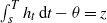 $\int_{s}^T h_{t} \,{\mathrm{d}} t-\theta =z$
. Let
 $z\gt0$
and let
 $h\in \Delta^s_z$
. The function
 \begin{align*}f(t)\, :\!= \, \int_{s}^t h_u \,{\mathrm{d}} u-\theta,\quad t\in [s,T] , \end{align*}
satisfies
 $\dot{f}=h$
a.e., and so
 \begin{align*}&(\Phi_0-\theta)\int_{s}^T h_t \,{\mathrm{d}} t+\dfrac{1}{2}\biggl(\int_{s}^T h_t \,{\mathrm{d}} t\biggr)^2+\dfrac{1}{2}\int_{s}^T h^2_t \,{\mathrm{d}} t\nonumber\\[3pt] &\quad \quad +\dfrac{1}{2} \int_{s}^T\biggl(\int_{s}^t h_v \,{\mathrm{d}} v-\theta\biggr)^2 \,{\mathrm{d}} t+\dfrac{\delta}{2}\int_{s}^T \biggl(\int_{t}^T h_v \,{\mathrm{d}} v\biggr)^2 \,{\mathrm{d}} t\\[3pt] &\quad =(\Phi_0-\theta)(z+\theta)+\dfrac{1}{2}(z+\theta)^2+\dfrac{1}{2}\int_{s}^T \dot{f}^2(t)\,{\mathrm{d}} t\\[3pt] &\quad \quad +\dfrac{1}{2}\int_{s}^T f^2(t) \,{\mathrm{d}} t+\dfrac{\delta}{2} \int_{s}^T (z-f(t))^2 \,{\mathrm{d}} t\\[3pt] &\quad =(\Phi_0-\theta)(z+\theta)+\dfrac{1}{2}(z+\theta)^2+\dfrac{1}{2}\dfrac {\delta (T-s)}{1+\delta}z^2\\[3pt] &\quad \quad +\dfrac{1}{2}\int_{s}^T \dot{f}^2(t)\,{\mathrm{d}} t+\dfrac{1}{2}(1+\delta)\int_{s}^T \biggl(f(t)-\dfrac{\delta z}{1+\delta}\biggr)^2 \,{\mathrm{d}} t.\end{align*}
Next, by applying Lemma 3.1 for
 \begin{align*}\alpha\, :\!= \, \sqrt{1+\delta},\quad g\, :\!= \, f-\frac{\delta z}{1+\delta}, \end{align*}
and observing the relations
 \begin{align*}g(s)=-\theta-\frac{\delta z}{1+\delta },\quad g(T)=\frac{z}{1+\delta}, \end{align*}
we get
 \begin{align*}&\min_{h\in \Delta^s_z}\biggl\{(\Phi_0-\theta)\int_{s}^T h_t \,{\mathrm{d}} t+\dfrac{1}{2}\biggl(\int_{s}^T h_t \,{\mathrm{d}} t\biggr)^2+\dfrac{1}{2}\int_{s}^T h^2_t \,{\mathrm{d}} t \nonumber\\[3pt] &\quad \quad +\dfrac{1}{2} \int_{s}^T\biggl(\int_{s}^t h_v \,{\mathrm{d}} v-\theta\biggr)^2 \,{\mathrm{d}} t+\dfrac{\delta}{2}\int_{s}^T \biggl(\int_{t}^T h_v \,{\mathrm{d}} v\biggr)^2 \,{\mathrm{d}} t\biggr\} \end{align*}
 \begin{align*} &\quad =(\Phi_0-\theta)(z+\theta)+\dfrac{1}{2}\ (z+\theta)^2+\dfrac{1}{2}\dfrac {\delta (T-s) }{1+\delta}z^2+\dfrac{1}{2}\dfrac{\sqrt{1+\delta}}{\sinh(\sqrt{1+\delta} (T-s))}(z+\theta)^2\\[3pt] &\quad \quad +\dfrac{1}{2}\sqrt{1+\delta}\tanh\biggl(\dfrac{\sqrt{1+\delta} (T-s)}{2}\biggr)\biggl(\biggl(\theta+\dfrac{\delta z}{1+\delta}\biggr)^2+\biggl(\dfrac{ z}{1+\delta}\biggr)^2\biggr)\\[3pt] &\quad =\Phi_0\theta+\dfrac{1}{2}\bigl(\sqrt{1+\delta}\coth((\sqrt{1+\delta} (T-s))-1\bigr)\theta^2\\[3pt] &\quad \quad +\biggl(\Phi_0+\dfrac{\delta\theta}{\sqrt{1+\delta}}\coth(\sqrt{1+\delta} (T-s))+\dfrac{\theta}{\sqrt{1+\delta}\sinh(\sqrt{1+\delta} (T-s))}\biggr)z\\[3pt] &\quad \quad +\dfrac{1}{2}\biggl(1+\dfrac {\delta (T-s) }{1+\delta}+\dfrac{\sqrt{1+\delta}}{\sinh(\sqrt{1+\delta} (T-s))}+\dfrac{1+\delta^2}{(1+\delta)^{3/2}}\tanh\biggl(\dfrac{\sqrt{1+\delta} (T-s)}{2}\biggr)\biggr)z^2.\end{align*}
Since
 $L^2[s,T]=\bigcup_{z\in\mathbb R}\Delta^s_z$
, then we are looking for a z which minimizes the above quadratic form. The minimum of the above quadratic is attained at the unique point
 \begin{align*}\hat z\, :\!= \, -\dfrac{\Phi_0+\frac{\delta\theta}{\sqrt{1+\delta}}\coth(\sqrt{1+\delta} (T-s))+\frac{\theta}{\sqrt{1+\delta}\sinh(\sqrt{1+\delta} (T-s))}}{1+\frac {\delta (T-s) }{1+\delta}+\frac{\sqrt{1+\delta}}{\sinh(\sqrt{1+\delta} (T-s))}+\frac{1+\delta^2}{(1+\delta)^{3/2}}\tanh\bigl(\frac{\sqrt{1+\delta} (T-s)}{2}\bigr)}. \end{align*}
Thus the unique solution to the optimization problem (3.1) is an element in
 $\Delta^s_{\hat z}$
. Simple calculations yield
 \begin{align*}\hat z+\theta=\dfrac{\bigl(1+\frac{1-\delta}{(1+\delta)^{3/2}}\tanh\bigl(\frac{\sqrt{1+\delta}(T-s)}{2}\bigr)+\frac {\delta (T-s) }{1+\delta}\bigr)\theta-\Phi_0}{1+\frac {\delta (T-s) }{1+\delta}+\frac{\sqrt{1+\delta}}{\sinh(\sqrt{1+\delta} (T-s))}+\frac{1+\delta^2}{(1+\delta)^{3/2}}\tanh\bigl(\frac{\sqrt{1+\delta} (T-s)}{2}\bigr)} \end{align*}
and (3.2) follows.
Finally, for the case where
 $\Phi_0=0$
, the minimal value of the above quadratic form (in z) is
 \begin{align*}&\dfrac{1}{2}(\sqrt{1+\delta}\coth(\sqrt{1+\delta} (T-s))-1)\theta^2\\[3pt] &\quad \quad -\dfrac{1}{2}\frac{\bigl(\frac{\delta}{\sqrt{1+\delta}}\coth(\sqrt{1+\delta} (T-s))+\frac{1}{\sqrt{1+\delta}\sinh(\sqrt{1+\delta} (T-s))}\bigr)^2\theta^2}{1+\frac {\delta (T-s) }{1+\delta}+\frac{\sqrt{1+\delta}}{\sinh(\sqrt{1+\delta} (T-s))}+\frac{1+\delta^2}{(1+\delta)^{3/2}}\tanh\bigl(\frac{\sqrt{1+\delta} (T-s)}{2}\bigr)}\\[3pt] &\quad =\dfrac{1}{2}\Biggl(\frac{\bigl(1+\frac {\delta (T-s) }{1+\delta}\bigr)\sqrt{1+\delta}\coth(\sqrt{1+\delta} (T-s))+\frac{1}{1+\delta}}{{1+\frac {\delta (T-s) }{1+\delta}+\frac{\sqrt{1+\delta}}{\sinh(\sqrt{1+\delta} (T-s))}+\frac{1+\delta^2}{(1+\delta)^{3/2}}\tanh\bigl(\frac{\sqrt{1+\delta} (T-s)}{2}\bigr)}}-1\Biggr)\theta^2\\[3pt] &\quad =\dfrac{1}{2}\mathcal V(T-s)\theta^2\end{align*}
where the last two equalities follow from direct computations.
Acknowledgements
I would like to thank the referees for their careful reading of the manuscript and for their insightful comments and suggestions, which have significantly improved the quality and clarity of the paper.
Funding information
Partially supported by the Israel Science Foundation (ISF) grant no. 305/25.
Competing interests
There were no competing interests to declare which arose during the preparation or publication process of this article.

 Open access

