2. PRELIMINARIES

In this section, we first recall the definitions of some well-known stochastic orders and then give the definitions of some notions of multivariate positive dependence.

Definition 2.1 (see Shaked and Shanthikumar [24, Chap. 1]): Let X and Y be two random variables with distribution functions F and G, respectively. Then X is said to be smaller than Y for the following:

(a) In the usual stochastic order, denoted by X ≤_st Y, if F(x) ≤ G(x) for all x, or if

for all increasing functions h

The relationships among these orders are shown in the following diagram (see, e.g., Shaked and Shanthikumar [24], Müller and Stoyan [20]):

A random vector X = (X₁,…,X_n) is said to be smaller than another random vector Y = (Y₁,…,Y_n) in the usual stochastic order, denoted by X ≤_st Y, if

holds for all increasing functions φ (see [24, Sect.4B]).

Let

be a product of totally ordered spaces

, endowed with the natural partial ordering. Let ψ₁, ψ₂ be two nonnegative functions defined on

, satisfying

where x ∨ y = (max(x₁,y₁),…,max(x_n,y_n)) and x ∧ y = (min(x₁,y₁),…,min(x_n,y_n)). Then we use the following notation:

Let X and Y be two n-dimensional random vectors with respective density functions f and g. X is said to be smaller than Y in the multivariate likelihood ratio order, denoted by X ≤_lr Y, if f [pr ]_TP2 g. It is well known that X ≤_lr Y implies X ≤_st Y (see Karlin and Rinott [14]).

There are several notions of multivariate positive dependence in the literature; see Barlow and Proschan [1] and Tong [27]. Here we review some among them. A function

is said to be multivariate totally positive of order 2 (MTP₂) if ψ [pr ]_TP2 ψ.

Definition 2.2: A random vector X = (X₁,X₂,…,X_n) is said to be the following:

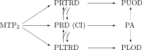
It is well known that MTP₂ implies CIS and CI, each of which, in turn, implies PA and that PA implies both PUOD and PLOD; see Barlow and Proschan [1] or Müller and Stoyan [20]. For n = 2, MTP₂ reduces to TP₂.

Harris [10] introduced the following two notions of multivariate dependence.

Definition 2.3: Let X be an n-dimensional random vector. Then X is said to be the following:

(a) right corner set increasing (RCSI) if

is increasing in z for all x

(b) left corner set decreasing (LCSD) if

is decreasing in z for all x

Lee [17] proved that if

is positive on a product space, then X is RCSI if and only if

is MTP₂ in x and that if

is positive on a product space, then X is LCSD if and only if

is MTP₂ in x. It is known from Block and Ting [5] that MTP₂ implies both RCSI and LCSD. Example 1 in Colangelo, Scarsini, and Shaked [6] illustrates that neither RCSI nor LCSD implies PA for n ≥ 3.

3. MULTIVARIATE NOTIONS OF POSITIVE DEPENDENCE

Three well-known notions of bivariate positive dependence are the stochastically increasing (SI), the right-tail increasing (RTI), and the left-tail decreasing (LTD); see Barlow and Proschan [1, Chap.5]. Given a random vector (X₁,X₂), X₂ is said to be the following:

• Stochastically increasing in X₁, denoted by SI(X₂|X₁), if
  
  is increasing in x₁ for all x₂
• Right-tail increasing in X₁, denoted by RTI(X₂|X₁), if
  
  is increasing in x₁ for all x₂
• Left-tail decreasing in X₁, denoted by LTD(X₂|X₁), if
  
  is decreasing in x₁ for all x₂

It is well known that SI implies both RTI and LTD, each of which, in turn, implies PA. Several notions of positive dependence were introduced in the literature to generalize SI, RTI, and LTD from the bivariate case to the multivariate case, which can be found in Colangelo et al. [6]. In this section, we introduce three notions of multivariate positive regression dependence generalizing bivariate notions of SI, RTI, and LTD.

For

and X = (X₁,…,X_n), let x_J and X_J denote a vector and a random vector constructed by using the coordinates in J ⊆ {1,…,n} of the indicated vectors, and let X_J ≤ x_J mean that X_j ≤ x_j for j ∈ J. The notations X_J = x_J and X_J > x_J have a similar interpretation.

Definition 3.1: Let X = (X₁,…,X_n) be a random vector. X is said to be the following:

The above notions of positive dependence reflect the intuition that if a set of positively dependent random variables is split into two subsets in some manner, then the random variables in two subsets tend to assume concordant values. For n = 2, PRD, PRTRD, and PLTRD reduce to SI, RTI, and LTD, respectively. Dubhashi and Ranjan [8] introduced the notions of negative regression dependence (NRD), negative left-tail regression dependence (NLTRD) and negative right-tail regression dependence (NRTRD) by reversing inequalities (3.1), (3.2), and (3.3) in Definition 3.1, and advocated their use as a simple and unifying paradigm for the analysis of random structures and algorithms. They claimed in their Proposition 24 [8] that the implication NRD ⇒ NLTRD and NRTRD is in the positive. However, the proof of their Proposition 24 is not correct. There is one big gap there. For occupancy numbers in the balls and bins experiment, their NRD property was proved by Dubhashi and Ranjan [8]. They also stated the NLTRD and NRTRD properties of occupancy numbers by their wrong Proposition 24. Hu and Xie [12] gave a detailed proof of the NLTRD and NRTRD properties of occupancy numbers with applications to dependence structure of order statistics.

We now investigate relationships between the above-defined notions.

Proposition 3.1: PRD [hArr ] CI.

Proof: By the definition of CI, it suffices to prove that X being CIS is equivalent to

for x₁ ≤ x₁*,…,x_k ≤ x_k* and k = 1,…,n − 1.

Fix k < n and let h(x_k+1,…,x_n) be an increasing function. For each i = k,…,n, define

Observe that

for i = k,…,n − 1. We claim that, due to (3.6), if h_i+1 is increasing, then h_i is also increasing. To see this, let x_j ≤ x_j* for j = 1,…,i. Then by (3.6),

where the first inequality follows from the increasing property of h_i+1 and the second one follows from the CIS property of X. From (3.5), we see that h_n is increasing. Therefore, h_k is increasing. This completes the proof. █

Proposition 3.2: MTP₂ ⇒ PRD, PLTRD, and PRTRD.

Proof: Since it is well known that MTP₂ implies CI (and hence PRD by Proposition 3.1), we only give the proof of the implication MTP₂ ⇒ PRTRD; the proof of the implication MTP₂ ⇒ PLTRD is similar. Let I and J be any two disjoint proper subsets of {1,…,n}. Without loss of generality, assume that I = {1,…,k} and J = {k + 1,…,n} with 1 ≤ k < n. Then the conditional density function of X_I, given X_J > x_J, is given by

where f is the density function of X and

is a normalizing constant. Similarly, the conditional density function of X_I, given X_J > x_J*, is

Fix x_J ≤ x_J* and notice that 1_[xJ,∞)(v_J) [pr ]_TP2 1_[xJ*,∞)(v_J), where 1_A denotes the indicator function of set A. Since f (x) is MTP₂ in x, it follows from Theorem 2.4 in Karlin and Rinott [14] that

and, hence, f₁(x_I) [pr ]_TP2 f₂(x_I). By Theorem 2.2 in [14], we get that f₁ ≤_st f₂; that is,

for all x_J ≤ x_J*. This completes the proof. █

It is seen that PRD implies PRTRD and PLTRD in the bivariate case and that neither PRTRD nor PLTRD implies PRD. However, the next counterexample illustrates that PRD does not imply PRTRD or PLTRD in the multivariate case.

Example 3.1 (PRD ⇒/ PRTRD or PLTRD for n ≥ 3; see Example 2 in [6]): Let (X₁,X₂,X₃) be a random vector with probability mass

at the points (−1,−1,0), (0,−1,0), (−1,0,1), (1,0,1), (0,2,2), and (1,2,2). It can be checked that X is PRD. However, X is not PRTRD or PLTRD, since

Example 3.1 also illustrates that PRD does not imply RCSI or LCSD. Example 3 in [6] shows that neither PRTRD nor PLTRD implies RCSI or LCSD. Furthermore, it can be checked that Example 1 in [6] shows that neither RCSI nor LCSD implies PRTRD or PLTRD. Therefore, there is no relationship among PRD, PRTRD, PLTRD, RCSI, and LCSD.

The relationships among these notions defined in Definitions 2.2 and 3.1 are summarized in Figure 1. It is still an open problem whether PRTRD or PLTRD implies PA.

Implications among some notions of positive dependence for n ≥ 3.

4. REGRESSION DEPENDENCE PROPERTIES IN LATENT VARIABLE MODELS

Let (T, Θ) be a latent variable model as described in Section 1. Throughout, assume that either Θ is absolutely continuous with respect to the Lebesgue measure on

, or that Θ is a discrete random variable. Let σ = σ₁ × σ₂ × ··· × σ_m denote a product measure on the support of Θ, where σ_i is the Lebesgue measure or the counting measure on the support of Θ_i, i = 1,…,m. We will generally use the abbreviations dσ_i(θ_i) = dθ_i and dσ(θ) = dθ without ambiguity.

4.1. Unidimensional Latent Variable Models

Theorem 4.1: Let (T,Θ) be a unidimensional latent variable model.

1. If

then T is PRTRD.

2. If

then T is PLTRD.

3. If

then T is PRD.

Proof: Part (3) follows from Corollary 1.1 and Proposition 3.2. We only give the proof of part (1), and the proof of part (2) is similar. To prove part (1), let I and J be any two disjoint proper subsets of {1,2,…,n} and let

be any increasing function. It suffices to prove that

Notice that

where G_Θ(·|t_J) is the conditional distribution function of [Θ|T_J > t_J]. On the other hand, it is easy to see from (4.1) and the conditional independence of T given Θ = θ that

is increasing [decreasing] in θ. So, to prove (4.4), we need to verify that

whenever t_J ≤ t_J′. In fact, denote by g_Θ(·|t_J) the conditional density or mass function of G_θ(·|t_J) and by g(θ) the density or mass function of Θ. Then

where

is a normalizing positive constant. Using the fact that the likelihood ratio order implies the hazard rate order, it follows from (4.1) that for any t_J ≤ t_J′,

is increasing [decreasing] in θ; that is, [Θ|T_J > t_J] ≤_lr [≥_lr] [Θ|T_J > t_J′] whenever t_J ≤ t_J′, which implies (4.6). This completes the proof. █

Assumptions (4.1), (4.2), and (4.3) in Theorem 4.1 cannot be replaced by the weaker assumption that

which can be seen from the following counterexample in Shaked and Spizzichino [25].

Example 4.1: Let ((T₁,T₂),Θ) be a unidimensional latent variable model with Θ taking on only two values, θ₁ and θ₂, where θ₁ < θ₂, and suppose that F₁(·|θ) = F₂(·|θ) = K(·|θ) for each θ. Denote

for i = 1,2 and assume that 0 < p < 1. Then the joint survival function of (T₁,T₂) can be written as

and, hence,

is increasing [decreasing] in η(t) = K₂(t)/K₁(t) for any fixed s if

Therefore, if T₁(θ₁) ≤_st [≥_st] T₁(θ₂), then

is increasing in t for any fixed s if and only if η(t) is increasing [decreasing] in t; that is, (T₁,T₂) is RTI if and only if T₁(θ₁) ≤_hr [≥_hr] T₁(θ₂).

From the argument in Example 4.1, we can easily get the following theorem, which states that assumptions (4.1), (4.2), and (4.3) are respectively necessary and sufficient conditions for T to be PRTRD, PLTRD, and PRD under the additional assumption that F_i(·|θ) does not depend on i and that G is an arbitrarily chosen distribution function of Θ. The proof is omitted here.

Theorem 4.2: Let (T,Θ) be a unidimensional latent variable model with F_i(·|θ) does not depend on i, and let G be the distribution function Θ. Then the following hold:

1. T is PRTRD for any G if and only if (4.1) holds.
2. T is PLTRD for any G if and only if (4.2) holds.
3. T is PRD for any G if and only if (4.3) holds.

4.2. Multidimensional Latent Variable Models

Theorem 4.1 will be generalized to the case that Θ is an m-dimensional random vector. The first result below gives sufficient conditions under which T is PRTRD.

Theorem 4.3: Let (T, Θ) be a multidimensional latent variable model with the conditional survival function of T_i(θ) being F_i(·|θ) for each i. If

(a)

(b) F_i(t|θ) is MTP₂ in θ for each t and i

(c) Θ is MTP₂,

then T is PRTRD.

Proof: Let I and J be any two disjoint proper subsets of {1,2,…,n} and let

be any increasing function. It follows that

where G_Θ(·|t_J) is the conditional distribution function of [Θ|T_J > t_J]. It is easy to see from (4.8) and the conditional independence of T, given Θ = θ, that

is increasing [decreasing] in θ. To prove that

is increasing in t_J, it suffices to prove that

We now turn to prove that

which implies (4.9).

Let h_Θ(·|t_J) and g(·) denote the density or mass functions of [Θ|T_J > t_J] and Θ, respectively. Then

where c(t_J) is a normalizing positive constant given by

Since a product of MTP₂ functions is still an MTP₂ function (see Proposition 3.3 in Karlin and Rinott [14]), it follows from assumptions (b) and (c) that g_Θ(θ|t_J) is MTP₂ in θ for each t_J. Let θ and θ′ be any two vectors in the support of Θ, and t_J ≤ t_J′. Then

implying (4.10), where the first inequality follows from the MTP₂ property of g_Θ(·|t_J) for each t_J and the second one follows from assumption (a). This completes the proof. █

By similar argument to that in the proof of Theorem 4.3, we can get the following two theorems concerning the dependence notions of PLTRD and PRD.

Theorem 4.4: Let (T, Θ) be a multidimensional latent variable model with the conditional distribution function of T_i(θ) being F_i(·|θ) for each i. If

(a)

(b) F_i(t|θ) is MTP₂ in θ for each t and i

(c) Θ is MTP₂,

then T is PLTRD.

Proof: The proof is similar to that of Theorem 4.3 with g_Θ(·|t_J), denoting the density or mass function of [Θ|T_J ≤ t_J], given by

where c(t_J) is a normalizing positive constant given by

This completes the proof. █

Theorem 4.5: Let (T, Θ) be a multidimensional latent variable model with the conditional density function of T_i(θ) being f_i(·|θ) for each i. If

(a)

(b) f_i(t|θ) is MTP₂ in θ for each t and i

(c) Θ is MTP₂,

then T is PRD.

Proof: The proof is similar to that of Theorem 4.3, with g_Θ(·|t_J), denoting the density or mass function of [Θ|T_J = t_J], given by

where c(t_J) is a normalizing positive constant given by

This completes the proof. █

For a componentwise separable latent variable model (T, Θ), assumption (b) in Theorems 4.3, 4.4, and 4.5 can be omitted.

5. APPLICATIONS

In this section, we give two applications of the results that were developed in previous sections. The applications are not exhaustive. There are several other interesting applications and examples given in Shaked and Spizzichino [25], Khaledi and Kochar [16], and Belzunce and Semeraro [3] to which the results in Section 4 can be applied.

5.1. Dependence Among Concomitants of Order Statistics

Let (X₁,Y₁),…,(X_n,Y_n) be a random sample of size n from a continuous bivariate distribution. If we arrange the X's in ascending order as X_1:n ≤ X_2:n ≤ ··· ≤ X_n:n, then the Y's associated with these order statistics are denoted by Y_[1],Y_[2],…,Y_[n] and are called concomitants of order statistics. They are also known as induced order statistics in the literature. Let F(·|x) denote the conditional distribution function of Y given X = x and let G denote the distribution function of Θ = (X_1:n,X_2:n,…,X_n:n). Then the distribution function of Y_[] = (Y_[1],Y_[2],…,Y_[n]) is given by

(see David and Nagaraja [7]); that is, (Y_[], Θ) is a componentwise separable latent variable model.

Khaledi and Kochar [15] obtained several results on dependence structure of Y_[] under different types of dependence between the parent random variables X and Y. Blessinger [4] extended some results in [15]. He proved that if (X,Y) is TP₂ or RR₂ (reverse regular of order 2) then Y_[] is MTP₂, and that if F(y|x) is TP₂ or RR₂ in (x,y), then Y_[] is RCSI. Similarly, if F(y|x) is TP₂ or RR₂ in (x,y), then Y_[] is LCSD. Recall that (X,Y) is RR₂ if and only if (X,−Y) is TP₂, and that a function ψ(x,y) is RR₂ if and only if ψ(x,−y) is TP₂ in (x,y). Notice that Θ is MTP₂ (see [14, Prop. 3.11]). By Proposition 3.2 and Theorems 4.3 and 4.4, we conclude the following.

Theorem 5.1:

1. If (X,Y) is TP₂ or RR₂, then Y_[] is PRD.

2. If F(y|x) is TP₂ or RR₂ in (x,y), then Y_[] is PRTRD.

3. If F(y|x) is TP₂ or RR₂ in (x,y), then Y_[] is PLTRD.

5.2. Dependence Among Concomitants of Record Values

Let {(X_i,Y_i),i ≥ 1} be a sequence of independent and identically distributed random vectors from a continuous bivariate distribution and let {Θ_n,n ≥ 1} be the sequence of upper record values of the sequence {X_i,i ≥ 1} with Θ₁ = X₁. Then the Y's associated with Θ_n are denoted by Y_[n] and is called the concomitant of the nth record value. Let F(·|x) denote the conditional distribution function of Y₁ given X₁ = x, and let W(·) and w(·) denote the survival function and the density function of X₁, respectively. It is well known that the joint density function of Θ = (Θ₁,…,Θ_n) is given by

and that the joint survival function of the concomitants Y_[] = (Y_[1],…,Y_[n]) is given by

(see Khaledi and Kochar [16]). Hence, (Y_[], Θ) is a componentwise separable latent variable model.

Khaledi and Kochar [16] proved that if (X,Y) is TP₂ or RR₂, then Y_[] TP₂ in pairs, and that if F(y|x) is TP₂ or RR₂ in (x,y), then H(y) is TP₂ in pairs. Similarly, if F(y|x) is TP₂ or RR₂ in (x,y), then H(y) is TP₂ in pairs. Since 1_{{θ1<θ2<···<θn}} is MTP₂ in θ, it follows from (5.1) that Θ is MTP₂. Therefore, by Theorems 4.3–4.5, we conclude that Theorem 5.1 also holds.