
 ϵ¯(Tl(λ),n,δ)



1. Introduction
Random sampling without replacement is prevalent across various scientific disciplines, including social sciences, computer sciences, and biology. Its applications span a wide range, from modeling gene mutations [Reference Lodato, Woodworth, Lee, Evrony, Mehta, Karger, Lee, Chittenden, D’Gama, Cai, Luquette, Lee, Park and Walsh30] and recommender systems [Reference Becchetti, Colesanti, Marchetti-Spaccamela and Vitaletti4] to analyzing social networks [Reference Casiraghi and Nanumyan8] and implementing variational clustering algorithms [Reference Sutter, Manduchi, Ryser and Vogt43]. In addition, beyond these traditional applications, random sampling can be employed for learning in cryptographic scenarios in which adversaries may exist. In cryptographic settings, when an adversarial player generates random variables [Reference Shamir41], these variables can be arbitrarily correlated. In contrast, as explained in Section 2, when a standard player generates random variables, they are subjected to the independent and identically distributed (i.i.d.) condition. Such cryptographic settings encompass numerous applications in quantum information processing that demand high-security requirements, such as blind-measurement-based quantum computation [Reference Hayashi and Morimae22] and quantum key distribution [Reference Hayashi and Tsurumaru23]. Moreover, similar settings are observed in machine learning, referred to as adversarial examples [Reference Bradley and Blossom7, Reference Chalé, Cox, Weir and Bastian9, Reference Dong, Liu and Shang15, Reference Gubri, Cordy, Papadakis, Traon and Sen20, Reference Levine and Feizi28, Reference Narodytska and Kasiviswanathan33]. In such settings, to estimate the behavior of the random variables, we need to employ random sampling without replacement. In addition, this kind of problem setting has been actively studied in the area of quantum information in several references (see [Reference Zhu and Hayashi46, Reference Zhu and Hayashi47] and references therein), while its essential part can be treated as a problem of statistics like the problem presented in this paper.
Random sampling without replacement is described by the hypergeometric distribution. It models the number of samples per group given a limited total number of samples. Since the selection of a single group element affects the probability of the remaining elements being drawn, the behavior of the random variable differs from that under the i.i.d. condition. Hypothesis testing provides a more logically complete structure to decision-making and therefore to better decisions. However, most existing studies on statistical hypothesis testing assume the i.i.d. condition, making them unsuitable for the adversarial setting mentioned previously. Although many papers have studied the behavior of observations under random sampling without replacement [Reference Ai, Kuželka and Wang1, Reference Bardenet and Maillard2, Reference Ben-Hamou, Peres and Salez5, Reference Chiu10–Reference Covey and Buonamano12, Reference Dey and Chaudhuri14, Reference Feng, Du, Gomes and Selman16, Reference Greene and Wellner18, Reference Greene and Wellner19, Reference Hodara and Reynaud-Bouret24, Reference Motoyama32, Reference O’Neill and Stern35, Reference Ouimet36, Reference Sambale and Sinulis38, Reference Serfling40, Reference Simon and Telle42, Reference Withers and Nadarajah45], only a limited number of works [Reference Bartroff, Lorden and Wang3, Reference Samohyl39] have addressed the problem under the framework of hypothesis testing. Therefore, to establish a logical decision-making framework in the above areas, it is necessary to study hypothesis testing under the hypergeometric distribution. In fact, while this setting is useful in the cryptographic setting, it can also be applied to other scenarios beyond the cryptographic setting that involve adversarial examples [Reference Bradley and Blossom7, Reference Chalé, Cox, Weir and Bastian9, Reference Dong, Liu and Shang15, Reference Gubri, Cordy, Papadakis, Traon and Sen20, Reference Levine and Feizi28, Reference Narodytska and Kasiviswanathan33]. In these scenarios, the adversarial case can be considered as a certain accidental case, and the i.i.d. case is considered as a certain non-accidental case.
In this paper we discuss one-sided hypothesis testing for random sampling without replacement. Assume that
 $n+1$
binary random variables
 $X_1, \ldots, X_{n+1}$
are generated according to random sampling without replacement. The task of this paper is to verify whether the expectation of the
 $(n+1)$
th binary random variable
 $X_{n+1}$
is smaller than a threshold
 $\epsilon$
when n observations
 $X_1, \ldots, X_{n}$
are given. We investigate this problem under the framework of statistical hypothesis testing, i.e. we study the upper confidence limit for the above expectation under a given significance level
 $\delta>0$
. In the case of random sampling with replacement, the optimal test has been well studied. In the optimal test, the decision should be made based on whether the count K of observed outcome 0 among
 $X_1, \ldots, X_{n}$
is greater than or less than a specific threshold
 $k(n,\delta)$
[Reference Lehmann and Romano27]. Only when K is equal to this threshold is a randomized decision necessary. This indicates that the benefit gained from employing a randomized decision is marginal.
Suppose that we have
 $n+m$
random variables
 $X_1,\ldots, X_{n+m}$
and n observations, and we are interested in the expectation of the remaining m variables. If both n and m go to infinity, we can use the normal approximation, which enables us to handle our problem in a way similar to the case with normal distribution. However, when random variables
 $X_1, \ldots, X_{n+1}$
are generated and we have only one remaining variable, we cannot use a normal approximation. Hypothesis testing in this case has not been sufficiently studied. This case requires us to discuss the problem in a different way. Such a problem setting occurs very frequently when we consider a cryptographic setting. In particular, the authors’ companion paper [Reference Li, Zhu and Hayashi29] applies the results obtained in this paper to the verification of blind quantum computation based on the relation pointed in [Reference Hayashi and Morimae22], although quantum key distribution is related to the case when n and m increase simultaneously [Reference Hayashi and Tsurumaru23]. In fact, the recent paper [Reference Li, Zhu and Hayashi29] derived the analysis of the verification of blind quantum computation based on the result of this paper. In addition, it is expected that the above-mentioned problem setting for hypothesis testing appears in adversarial machine learning [Reference Shamir41].
In this paper, to address the problem mentioned above, we introduce a randomized test that makes a randomized decision using a randomization parameter
 $0 \leq \lambda < 1 $
when the outcome K is greater than a certain threshold l. That is, our randomized test makes a deterministic decision when the outcome K is not greater than the threshold l. This randomized test with parameter
 $0 < \lambda < 1$
significantly improves the performance over the deterministic test. For example, when the significance level
 $\delta>0$
is exponentially small in n, the upper confidence limit for the expectation of
 $X_{n+1}$
is always the trivial value 1, i.e. any deterministic test cannot provide a non-trivial value. However, our randomized test provides a non-trivial value for the upper confidence limit even with an exponentially small significance level
 $\delta$
in n. We study the asymptotic behavior of the performance of this new randomized test under two regimes, depending on the behavior of the threshold l. One is the constant regime in which the threshold l remains a constant. The other is the linear regime in which the threshold l increases in proportion to n. Under both regimes, we show that our randomized tests outperform the deterministic test significantly.
The rest of this paper is organized as follows. Section 2 explains the relation between our problem setting and the cryptographic setting. Section 3 formulates our problem setting and introduces our new randomized test based on the randomization parameter
 $0 \leq \lambda < 1$
. Some preliminary results that demonstrate the randomized test’s advantages are also presented in Section 3, with detailed proofs deferred to Section 4. Section 5 presents the first main result (Theorem 1) of this paper, which clarifies the asymptotic behaviors of our randomized test under the linear regime. Section 6 considers the power, i.e. the probability of detecting a given upper confidence limit for the i.i.d. case under this regime. Section 7 presents the second main result (Theorem 2) of this paper, which clarifies the asymptotic behaviors of our randomized test under the constant regime. Section 8 proposes a new method for computing the upper confidence limit, with its analytical expression provided in Theorem 3. This result is pivotal to the proofs of our main results in Sections 5 and 7. Section 9 presents a brief proof of the theorem stated in Section 5. Section 10 gives the conclusion. Several auxiliary lemmas are presented in Appendices A and B. Many technical results are also presented in the appendices.
2. Relation with Cryptographic Setting
The research topics in cryptography are not limited to secret message transmission; message authentication is also a major focus in this field. Any message authentication process involves a decision-making step to determine whether a received document should be accepted or rejected, as we need to consider two scenarios, the honest case and the dishonest case, where the latter is often referred to as the adversarial case. Beyond message authentication, it is often required to distinguish the honest case and the dishonest case in the cryptographic setting. For example, in the verification of quantum computation [Reference Li, Zhu and Hayashi29, Reference Morimae, Takeuchi and Hayashi31, Reference Zhu and Hayashi46, Reference Zhu and Hayashi47], there are two players, Alice and Bob, with Bob preparing part of the quantum computing device for Alice to use. Assume that Alice does not trust Bob, then she must measure the part provided by Bob to verify whether he has prepared it honestly. This kind of problem setting is formulated in the following general way.
In the honest case, the original random variables
 $X_1, X_2, \ldots, X_{n+1}$
satisfy the i.i.d. condition. In the dishonest case, these variables do not satisfy this condition. In the latter scenario, it is presumed that the adversary has artificial control over these random variables. As such, our decision-making process must account for the dishonest case. The cryptographic scenario imposes the following two requirements on our decision-making approach [Reference Morimae, Takeuchi and Hayashi31].
The first requirement is soundness, which ensures the quality of the remaining variable
 $Y_{n+1}$
(whose formal definition is given in Section 3) under the condition that the test is passed and the dishonest case is assumed. Since we consider ‘under the condition’, we need to guarantee that the conditional probability
 $\textrm{P} (Y_{n+1} =1|\operatorname{Pass})$
is smaller than a certain threshold. This is because we are interested in the objective probability only when the test is passed. In the case of a one-sided test, soundness is guaranteed by the upper (or lower) confidence limit of the parameter of interest under a given significant level. In other words, this part corresponds to the calculation of the minimum significant level to guarantee a given upper confidence limit, which is often called the p-value for the upper confidence limit.
The second requirement is completeness, which means that the test is passed with a high probability in the honest case when the probability
 $\textrm{P}(X_i=1)$
is sufficiently small. The completeness is guaranteed by the power. Therefore, we discuss the power of our test only in the honest case.
3. Problem Setting
3.1. Formulation
We consider
 $n+1$
binary random variables
 $X_1, \ldots, X_{n+1}$
that take values in
 $\{0,1\}$
and are subject to a joint distribution
 $P_{X_1, \ldots, X_{n+1}}$
. By randomly drawing n samples
 $Y_1, \ldots, Y_n$
without replacement from
 $X_1, \ldots, X_{n+1}$
, we would like to estimate the marginal distribution of the remaining binary variable
 $Y_{n+1}$
. To characterize this problem, we introduce the set
 $S_{n+1}$
of permutations on
 $[n+1]\,:\!=\,\{1, \ldots, n+1\}$
. The joint distribution
 $P_{Y_1, \ldots, Y_{n+1}}$
of
 $Y_1, \ldots, Y_{n+1}$
is given as
 \begin{align*}P_{Y_1, \ldots, Y_{n+1}}(y_1, \ldots, y_{n+1})=\sum_{\sigma \in S_{n+1}}\frac{1}{(n+1) ! }P_{X_{\sigma(1)}, \ldots, X_{\sigma(n+1)}}(y_1, \ldots, y_{n+1}).\end{align*}
Denote the set of permutation invariant distributions on
 $[n+1]$
by
 ${\mathcal Q}_{n+1}$
, then the joint distribution
 $P_{Y_1, \ldots, Y_{n+1}}$
can be considered as an arbitrary element of
 ${\mathcal Q}_{n+1}$
.
Our problem setting is formulated as follows. Suppose n observed variables
 $Y_1, \ldots, Y_n$
are
 $y_1, \ldots, y_n$
, our task is to estimate the conditional distribution
 $P_{Y_{n+1}| (Y_1, \ldots, Y_n) =(y_1, \ldots, y_n)}$
. For each observed variable
 $Y_i$
, the observation outcome
 $Y_i=0$
is labeled as a ‘success’ and the outcome
 $Y_i=1$
is labeled as a ‘failure’. Since
 $P_{Y_1, \ldots, Y_{n+1}}$
is permutation invariant, the above conditional distribution
 $P_{Y_{n+1}| Y_1, \ldots, Y_n}$
depends only on the random variable K that describes the number of failures among the n observations
 $Y_1, \ldots, Y_n$
. Hence, we discuss only the conditional distribution
 $P_{Y_{n+1}|K}$
. Since
 $Y_{n+1}$
is a binary variable taking values in
 $\{0,1\}$
, it suffices to estimate the conditional probability
 $\textrm{P}(Y_{n+1}=1|K \le k)$
for each realization k.
Now, we discuss this problem in the framework of one-sided hypothesis testing with significance level
 $\delta$
. The problem setting is formulated as follows. We are interested in the probability of
 $Y_{n+1}=1$
under the condition that our test is passed. That is, we focus on the conditional distribution
 $\textrm{P}(Y_{n+1}=1| \operatorname{Pass} )$
, where ‘
 $\operatorname{Pass}$
’ means the case that our test is passed. The aim of our test is to guarantee that the conditional probability
 $\textrm{P}(Y_{n+1}=1| \operatorname{Pass} )$
is not greater than a threshold
 $\epsilon$
with significance level
 $\delta$
. Hence, when its upper bound
 $\epsilon$
is given, the null hypothesis
 $H_0$
and the alternative hypothesis
 $H_1$
are given as
 \begin{align*}H_0\,:\, &\quad \textrm{P}(Y_{n+1}=1| \operatorname{Pass} ) > \epsilon, \\H_1\,:\, &\quad \textrm{P}(Y_{n+1}=1| \operatorname{Pass} ) \le \epsilon.\end{align*}
In this problem setting, it is needed to set the event ‘Pass’ as follows: when the test is passed, the null hypothesis
 $H_0$
is rejected. This is because we are required to guarantee the alternative hypothesis
 $H_1$
under the event ‘Pass’. Due to the above requirement and the correlation between
 $Y_{n+1}$
and
 $Y_1, \ldots, Y_n$
, the forms of our hypotheses depend on our decision.
In other words, the expectation
 $\textrm{E}[Y_{n+1}]$
does not equal
 $\textrm{P} (Y_{n+1} =1|\operatorname{Pass})$
. This point is the difficulty of our problem. Given a test T, the maximum of the conditional probability
 $\textrm{P}(Y_{n+1}=1| \operatorname{Pass} T)$
with significance level
 $\delta$
is given as
 \begin{align*}\overline{\epsilon}(T,n,\delta)\,:\!=\,\max_{Q \in {\mathcal Q}_{n+1}}\{Q(Y_{n+1}=1| \operatorname{Pass} T)|Q(\operatorname{Pass} T) \ge \delta \}.\end{align*}
Since we can guarantee that the conditional probability
 $\textrm{P}(Y_{n+1}=1| \operatorname{Pass} T)$
is not greater than the maximum, the above maximum is simply called the upper confidence limit at significance level
 $\delta$
. In this case, we can say that
 $\delta$
is the p-value of the upper bound
 $\overline{\epsilon}(T,n,\delta)$
of the conditional probability
 $\textrm{P}(Y_{n+1}=1| \operatorname{Pass} T)$
.
The most natural choice for the rejection region of the null hypothesis
 $H_0$
is the set
 $\{K| K \leq k\}$
, i.e. the test is passed when
 $K \le k$
. This rejection region is determined by the threshold value k. We denote this deterministic test by
 $T_k$
. Under this choice of the rejection region, the upper confidence limit is given as
 \begin{align*}\overline{\epsilon}(T_k,n,\delta)=\max_{Q \in {\mathcal Q}_{n+1}}\{Q(Y_{n+1}=1|K \le k)\,|\, Q(K \le k) \ge \delta \}.\end{align*}
That is, we can guarantee that the conditional probability
 $\textrm{P}(Y_{n+1}=1 |K \le k)$
is not greater than the upper confidence limit
 $\overline{\epsilon}(T_k,n,\delta)$
at significance level
 $\delta$
. Here the threshold k denotes the number of allowed failures.
As we show in Section 4.1, the upper confidence limit
 $\overline{\epsilon}(T_k,n,\delta)$
reads
 \begin{align}\overline{\epsilon}(T_k,n,\delta)=\left\{\begin{array}{l@{\quad}c}\dfrac{(k+1) (n+1-k) -\delta(n+1)}{\delta(n-k)(n+1)} &\hbox{ when } \delta \ge \dfrac{k+1}{n+1}, \\[6pt]1&\hbox{ when }\delta < \dfrac{k+1}{n+1} .\end{array}\right.\end{align}
Equation (1) shows that when the significance level
 $\delta$
is smaller than
 $1/(n+1)= \min_{k \ge 0} ((k+1)/(n+1))$
, we cannot make any non-trivial upper confidence limit for the conditional probability
 $\textrm{P}(Y_{n+1}=1|K \le k)$
for any integer
 $k=0,1,\ldots, n$
. Therefore, it is impossible to realize an exponentially small significance level with respect to n for any non-trivial upper confidence limit. In other words, when we set the significance level
 $\delta$
to be an exponentially small value with respect to n, the upper confidence limit becomes 1.
Fortunately, this problem can be resolved by introducing a randomized test. Our randomized test is not a trivial idea. To see the strength of our method, we first see a usual randomized test as follows. When we consider a randomized test, usually we make the randomization only on the threshold. Consider the following test. When
 $K \le k-1$
, we reject the null hypothesis
 $H_0$
. When
 $K \ge k+1$
, we adopt the null hypothesis
 $H_0$
. When
 $K = k$
, we reject the null hypothesis
 $H_0$
with probability
 $1-\lambda$
, and adopt
 $H_0$
with probability
 $\lambda$
. This test can be considered as a probabilistic mixture of the test
 $T_k$
and
 $T_{k-1}$
with probabilities
 $1-\lambda $
and
 $\lambda$
. We denote this test by
 $\tilde{T}_k(\lambda)$
. Since
 $\tilde{T}_k(0)=T_k$
, this method is a generalization of the above method. As we show in Section 4.2, the upper confidence limit
 $\overline{\epsilon}(\tilde{T}_k(\lambda),n,\delta)$
reads
 \begin{align}\overline{\epsilon}(\tilde{T}_k(\lambda),n,\delta)&=\left\{\begin{array}{l@{\quad}l}\xi_1(n,k,\lambda,\delta) &\hbox{ when }\delta\ge (1-\lambda) +\lambda \dfrac{k}{n+1}, \\[3pt]\xi_2(n,k,\lambda,\delta) &\hbox{ when }(1-\lambda) +\lambda \dfrac{k}{n+1} > \delta\ge (1-\lambda) \dfrac{k+1}{n+1}, \\[3pt]1&\hbox{ when }(1-\lambda) \dfrac{k+1}{n+1}> \delta ,\end{array}\right.\end{align}
where
 \begin{align*}\xi_1(n,k,\lambda,\delta) &\,:\!=\, \frac{(k-1)\lambda(n+1-k)+(n+1)(1-\delta)}{\delta(n+1)\lambda(n+1-k)},\\[3pt]\xi_2(n,k,\lambda,\delta) &\,:\!=\, \frac{\delta(n+1) (k-(1-\lambda)(k+1))+(1-\lambda)^2 (k+1) (n+1-k)}{\delta(n+1)(k+(1-\lambda) (n-2k))}.\end{align*}
Consequently, with this type of randomized test, when we set the significance level
 $\delta$
to be an exponentially small value with respect to n, the upper confidence limit
 $\overline{\epsilon}(\tilde{T}_k(\lambda),n,\delta)$
becomes 1. To see this, we examine two cases depending the behavior of
 $\lambda$
. First, if
 $(1-\lambda) (k+1)/(n+1)> \delta$
then the above observation holds immediately. Second, if
 $(1-\lambda) +\lambda {k}/{(n+1)} > \delta\ge (1-\lambda) (k+1)/(n+1)$
then
 $(1-\lambda)$
is also an exponentially small value with respect to n, leading to that
 $\overline{\epsilon}(\tilde{T}_k(\lambda),n,\delta)=\xi_2(n,k,\lambda,\delta)$
converges to 1. This discussion shows that a more advanced randomization is needed for further improvement.
The above randomized test makes a randomized decision only when the observation is the threshold value. In contrast, our method makes this kind of randomized decision for all observations, and the probability of this randomization depends on our observation. To introduce our randomized test, which is different from the above randomized test, we consider the following artificial noise before our data processing. Instead of
 $Y_1, \ldots, Y_{n}$
, we focus on n variables
 $U_1, \ldots, U_{n}$
with the following conditional distribution
 $P_{U_i|Y_i}$
:
 \begin{align}P_{U_i|Y_i}(0|0)=1, \quad P_{U_i|Y_i}(1|0)=0 ,\quad P_{U_i|Y_i}(0|1)=\lambda, \quad P_{U_i|Y_i}(1|1)=1-\lambda ,\end{align}
where
 $0 \leq \lambda < 1$
is a randomization parameter. For convenience, we define
 $\nu\,:\!=\,1-\lambda$
. The outcome
 $U_i=0$
is labeled as a ‘success’ and the outcome
 $U_i=1$
is labeled as a ‘failure’. Denote the number of failures among
 $U_1, \ldots, U_{n}$
by the random variable L, which satisfies the following conditional distribution
 $P_{L|K}$
:
 \begin{align*}P_{L|K}(l|k)=\left\{\begin{array}{l@{\quad}l}0 & {\rm when}\,\, l > k, \\\left(\begin{smallmatrix} k \\ l \end{smallmatrix}\right) \lambda^{k-l} (1-\lambda)^{l}& {\rm when}\,\, l \le k,\end{array}\right. \end{align*}
which implies that
 $L \le K$
. Then, we define the following test by using the random variable L instead of K. When
 $L \le l$
, we reject the null hypothesis
 $H_0$
. When
 $L \ge l+1$
, we adopt the null hypothesis
 $H_0$
. We denote this test by
 $T_l(\lambda)$
, in which the threshold l denotes the number of allowed failures.
Then, the upper confidence limit
 $\overline{\epsilon}(T_l(\lambda),n,\delta)$
is calculated as
 \begin{align*}\overline{\epsilon}(T_l(\lambda),n,\delta)=\max_{Q \in {\mathcal Q}_{n+1}}\{Q(Y_{n+1}=1|L \le l)\,|\, Q(L \le l) \ge \delta \}.\end{align*}
When
 $K \le l$
, the relation
 $L\le K$
guarantees that the probability
 $\textrm{P}(Y_{n+1}=1)$
under the observed condition is not greater than the upper limit. Otherwise, we make a randomized decision. Note that
 $\overline{\epsilon}(T_l,n,\delta)$
is the special case of
 $\overline{\epsilon}(T_l(\lambda),n,\delta)$
with
 $\lambda=0$
. This method guarantees that the conditional probability
 $\textrm{P}(Y_{n+1}=1|L \le l)$
is not greater than
 $\overline{\epsilon}(T_l(\lambda),n,\delta)$
at significance level
 $\delta$
.
The one-sided hypothesis testing introduced above plays a crucial role in the task of verifying quantum states in the adversarial scenario (QSVadv) [Reference Zhu and Hayashi46, Reference Zhu and Hayashi47]. In QSVadv, one aims to ensure that the quantum state on one system has sufficiently high fidelity with the target state by performing n measurements on other systems. So far, only the verification protocol with
 $l=0$
has been studied in the literature. The performance with general
 $l>0$
is still not clear.
To see how our new method with
 $\lambda>0$
can achieve exponentially small significance level, we set
 $l=0$
. For
 $z\in\{0,1,\dots,n+1\}$
, let
 $\delta=\delta_z\,:\!=\,({(n+1-z)\lambda^z+ z \lambda^{z-1}})/({n+1})$
, then we have
 \begin{align}\overline{\epsilon}(T_0(\lambda),n,\delta_z)=\frac{z}{z+(n-z+1)\lambda}. \end{align}
Equation (4) follows from (57) in Ref. [Reference Zhu and Hayashi47], and a simple proof is also given in Section 4.3. Since
 $\delta_z$
has a similar behavior as
 $\lambda^z$
, this equation shows that the above randomized test can realize a non-trivial statement even with an exponentially small significance level. So randomized tests can significantly outperform deterministic tests.
By contrast, randomized tests are not necessary to achieve an exponentially small significance level for i.i.d. variables. To see this, we define the upper confidence limit for the i.i.d. case and a test T as
 \begin{align*}\overline{\epsilon}_{\textrm{i.i.d.}}(T,n,\delta)\,:\!=\,\max_{Q \in {\mathcal Q}_{\operatorname{i.i.d.},n+1}}\{Q(Y_{n+1}=1| \operatorname{Pass} T) \,|\, Q(\operatorname{Pass} T) \ge \delta \},\end{align*}
where
 ${\mathcal Q}_{\textrm{i.i.d.},n+1} $
is the set of independent and identical distributions on
 $[n+1]$
. Then, for the deterministic test
 $T_k$
, we have
 \begin{align}\overline{\epsilon}_{\textrm{i.i.d.}}(T_k,n,\delta)=&\max_{Q \in {\mathcal Q}_{\operatorname{i.i.d.},n+1}}\{Q(Y_{n+1}=1|K \le k)\,|\, Q(K\le k) \ge \delta \} .\end{align}
We denote by
 $P_{\theta}^{n+1}$
the independent and identical distribution on
 $[n+1]$
where the probability of the event
 $Y_i=1$
is
 $\theta$
. Hence,
 ${\mathcal Q}_{\textrm{i.i.d.},n+1} $
can be written as
 $\{P_{\theta}^{n+1}\}_{\theta \in [0,1]}$
, which implies that
 \begin{align}\overline{\epsilon}_{\textrm{i.i.d.}}(T_k,n,\delta)=&\max_{\theta \in [0,1]} \{\theta \,|\, P_{\theta}^{n+1}(K\le k) \ge \delta \} .\end{align}
As we show in Sections 5 and 7,
 $\overline{\epsilon}_{\textrm{i.i.d.}}(T_k,n,\delta)$
has a non-trivial value even when the significance level
 $\delta$
is exponentially small with respect to n.
3.2. Frequently used notation
In preparation for further discussions, here we introduce further notation, which will be frequently used throughout the paper.
Let
 $\mathbb{Z}^{\geq j}$
be the set of integers larger than or equal to j. For
 $0 \leq p \leq 1$
and
 $z,l,j\in\mathbb{Z}^{\geq 0}$
, let
 \begin{align} b_{z,j}(p)\,:\!=\, \binom{z}{j} p^j (1-p)^{z-j},\qquad B_{z,l}(p)\,:\!=\, \sum_{j=0}^l b_{z,j}(p)= \sum_{j=0}^l \binom{z}{j} p^j (1-p)^{z-j}.\end{align}
Here it is understood that
 $b_{z,j}(p)=0$
whenever
 $j\geq z+1$
, and
 $x^0=1$
even if
 $x=0$
. When there is no danger of confusion, we shall use
 $b_{z,l}$
and
 $B_{z,l}$
as shorthand for
 $b_{z,l}(\nu)$
and
 $B_{z,l}(\nu)$
, respectively. Define
 \begin{align} \Delta_{z,l}\,:\!=\,B_{z,l}-B_{z+1,l},\quad z,l=0,1,2,\ldots.\end{align}
For
 $0 < \delta\leq 1$
, define
 \begin{align} z^*(l,\delta,\lambda)\,:\!=\,\min\{z\in\mathbb{Z}^{\geq l}|B_{z,l}\leq \delta\},\quad z_*(l,\delta,\lambda)\,:\!=\,z^*(l,\delta,\lambda)-1.\end{align}
Here
 $z^*(l,\delta,\lambda)$
and
 $z_*(l,\delta,\lambda)$
are well defined because
 $B_{l,l}(\nu)=1$
,
 $\lim_{z\to\infty} B_{z,l}(\nu)=0$
, and that
 $B_{z,l}(\nu)$
is non-increasing in z for
 $z\geq l$
according to Lemma 7. In this paper we shall frequently use
 $z^*$
and
 $z_*$
as shorthand for
 $z^*(l,\delta,\lambda)$
and
 $z_*(l,\delta,\lambda)$
, respectively.
The standard normal density function and its distribution function read
 \begin{align} \phi(x)\,:\!=\,\frac{1}{\sqrt{2\pi}}\mathrm{e}^{-x^2/2},\quad \Phi(x)\,:\!=\,\int_{-\infty}^x \phi(t) \,\textrm{d} t.\end{align}
The function
 $\Phi^{-1}(x)$
is defined as the inverse function of
 $\Phi(x)$
.
For
 $0< p,q<1$
, the relative entropy between two binary non-negative vectors
 $(p,1-p)$
and
 $(q,1-q)$
reads
 \begin{align} D(p\|q)\,:\!=\,p\ln\frac{p}{q}+(1-p)\ln\frac{1-p}{1-q}.\end{align}
For
 $\gamma\geq0$
and
 $0<x<1$
, define
 $t_\mathrm{D}(\gamma,x)$
as the unique solution of t to the equation
 \begin{align} t D\!\left( \frac{\gamma}{t}\Big\|x\right) =1, \quad t\geq \frac{\gamma}{x}.\end{align}
Note that
 $t_\mathrm{D}(\gamma,x)$
is well defined because
 $D(x\|x)=0$
,
 $D(0\|x)=-\ln(1-x)$
, and that
 $D( \gamma/t\|x)$
is non-decreasing in t for
 $t\geq \gamma/x$
thanks to Lemma 12 in Appendix A.2. For
 $0 \leq s < 1$
and
 $r>0$
, define
 $\epsilon_D(s,r)$
as the unique solution of
 $\epsilon$
to the equation
 \begin{align} r=D(s\|\epsilon ), \quad 0 \leq s \leq \epsilon < 1 .\end{align}
Similarly, for
 $0 < \epsilon<1$
and
 $0 < r \leq- \ln(1-\epsilon)$
, define
 $s_D(\epsilon,r)$
as the unique solution of s to (13). Both
 $\epsilon_D(s,r)$
and
 $s_D(\epsilon,r)$
are well defined according to Lemma 12 in Appendix A.2.
For
 $x\geq 0$
and
 $k\in\mathbb{Z}^{\geq 0}$
, the Poisson cumulative distribution function reads
 \begin{align} \mathrm{Pois}(k,x)\,:\!=\,\mathrm{e}^{-x} \sum_{j=0}^k \frac{x^j}{j!}.\end{align}
For
 $0 < \delta < 1$
and
 $k\in\mathbb{Z}^{\geq 0}$
, define
 $t_\mathrm{P}(k,\delta)$
as the unique solution of t to the equation
 \begin{align}\mathrm{Pois}(k,t) = \delta \quad \hbox{for } \ t\geq 0.\end{align}
Note that
 $t_\mathrm{P}(k,\delta)$
is well defined because
 $\mathrm{Pois}(k,0)=1$
,
 $\lim_{t\to\infty}\mathrm{Pois}(k,t)=0$
, and that
 $\mathrm{Pois}(k,t)$
is monotonically decreasing in t for
 $t\geq0$
according to Lemma 13 in Appendix A.3.
3.3. Properties of the upper confidence limit
Here we summarize some basic properties of the upper confidence limit. In particular, Proposition 1 clarifies the monotonicities of
 $\overline{\epsilon}_{\operatorname{i.i.d.}}(T_k,n,\delta)$
, and Lemma 1 provides useful bounds for
 $\overline{\epsilon}(T_k,n,\delta)$
,
 $\overline{\epsilon}(T_l(\lambda),n,\delta)$
, and
 $\overline{\epsilon}_{\textrm{i.i.d.}}(T_k,n,\delta)$
. The monotonicities of
 $\overline{\epsilon}(T_l(\lambda),n,\delta)$
will be clarified later in Proposition 6 after several preparations. Proposition 1 and Lemma 1 are proved in Appendices C and D, respectively.
Proposition 1. Suppose
 $0 < \delta\leq1$
,
 $n,k\in\mathbb{Z}^{\geq 0}$
, and
 $n>k$
. Then
 $\overline{\epsilon}_{\operatorname{i.i.d.}}(T_k,n,\delta)$
is non-increasing in
 $\delta$
for
 $0 < \delta\leq1$
, non-increasing in n for
 $n\geq k+1$
, and non-decreasing in k for
 $0 \leq k\leq n-1$
.
Lemma 1. Suppose
 $0 < \delta \leq \tfrac12$
,
 $k,l,n\in \mathbb{Z}^{\geq 0}$
,
 $n>k$
,
 $n>l$
. In the i.i.d. case, we have
 \begin{align}\overline{\epsilon}_{\textrm{i.i.d.}}(T_k,n,\delta) \ge\overline{\epsilon}_{\textrm{i.i.d.}}\left(T_k,n,\frac12\right) > \frac{k}{n}.\end{align}
As a generalization, for
 $0 \leq \lambda < 1$
we have
 \begin{align}\overline{\epsilon}(T_l(\lambda),n,\delta)\ge\overline{\epsilon}\left(T_l(\lambda),n,\frac12\right)\left\{\begin{array}{l@{\quad}l} =1 &\quad when \,\, l\geq \nu n ,\\ > \frac{l}{\nu n}&\quad when\,\, l<\nu n.\end{array}\right.\end{align}
For
 $\lambda=0$
and
 $k/n<\delta\leq \tfrac12$
, we have
 \begin{align}\overline{\epsilon}(T_k,n,\delta) > \frac{k}{n\delta}.\end{align}
4. Proofs of Simple Key Relations
4.1. Proof of (1)
Let
 $Q_{j}$
be the permutation invariant distribution of variables
 $Y_1, Y_2,\ldots, Y_{n+1}\in\{0,1\}$
that satisfy
 $\sum_{i=1}^{n+1}Y_i=j$
. Then any element of
 $ {\mathcal Q}_{n+1}$
can be written in the form
 $Q[\vec{p}]\,:\!=\,\sum_{j=0}^{n+1}p_j Q_j$
, where
 $\vec{p}\,:\!=\,(p_j)_{j=0}^{n+1}$
. In addition, we have
 \begin{align*}Q_j(K=k)=\left\{\begin{array}{l@{\quad}l}\dfrac{n+1-j}{n+1}& \hbox{ when } k=j, \\[6pt]\dfrac{j}{n+1} & \hbox{ when } k=j-1, \\[6pt]0 & \hbox{ otherwise} .\end{array}\right.\end{align*}
It follows that
 \begin{align}Q[\vec{p}](K \le k)&=\sum_{j=0}^k p_j + \frac{k+1}{n+1}p_{k+1}\end{align}
 \begin{align} Q[\vec{p}](Y_{n+1}=1,K \le k)&=\sum_{j=0}^k \frac{j}{n+1}p_j+ \frac{k+1}{n+1}p_{k+1},\end{align}
and
 \begin{align}\overline{\epsilon}(T_k,n,\delta)=&\max_{(p_j)_{j=0}^{n+1}}\bigg\{\dfrac{Q[\vec{p}](Y_{n+1}=1,K \le k)}{Q[\vec{p}](K \le k)}\,\bigg|\,Q[\vec{p}](K \le k)\ge \delta\bigg\}\nonumber\\[6pt]\stackrel{(a)}{=}&\max_{0 \le p_k \le 1 }\bigg\{\frac{p_k\dfrac{k}{n+1} +\dfrac{k+1}{n+1}(1- p_{k})}{p_k + \dfrac{k+1}{n+1}(1-p_{k})}\,\bigg|\, p_k + \dfrac{k+1}{n+1}(1-p_{k}) \ge \delta\bigg\}\nonumber\\[6pt]=&\max_{0 \le p_k \le 1 }\bigg\{\dfrac{ k+1 -p_k}{(k+1)+ p_k(n-k)}\,\bigg|\, \dfrac{(k+1)+ p_k(n-k)}{n+1}\ge \delta\bigg\}.\end{align}
To derive (a) above, we use (19), (20), and choose
 $p_1, \ldots, p_{k-1}$
to be zero. When
 $(k+1)/(n+1)> \delta$
, the maximum in (21) is realized with
 $p_k=0$
, i.e. the maximum is 1. When
 $(k+1)/(n+1)\le \delta$
, the maximum is realized with
 $p_k=((n+1)\delta-(k+1))/(n-k)$
, i.e. the maximum is
 $((k+1)(n-k+1)-\delta(n+1))/[\delta(n+1)(n-k)]$
. Then, we have (1).
4.2. Proof of (2)
The test
 $\tilde{T}_k(\lambda)$
satisfies that
 \begin{align*}Q[\vec{p}](\operatorname{Pass} \tilde{T}_j(\lambda))&=(1-\lambda) \left( \sum_{j=0}^k p_j + \frac{k+1}{n+1}p_{k+1} \right)+\lambda\left( \sum_{j=0}^{k-1} p_j + \frac{k}{n+1}p_{k} \right) \nonumber\\&= \sum_{j=0}^{k-1} p_j+\left( 1-\lambda + \frac{k}{n+1}\lambda\right) p_k+ \frac{k+1}{n+1} (1-\lambda) p_{k+1}=\sum_{j=0}^{k+1} a_j p_j ,\\Q[\vec{p}](Y_{n+1}=1,\operatorname{Pass} \tilde{T}_j(\lambda))&=(1-\lambda) \sum_{j=0}^{k+1} \frac{j}{n+1}p_j+\lambda \sum_{j=0}^k \frac{j}{n+1} p_j \nonumber\\&=\sum_{j=0}^k \frac{j}{n+1}p_j+ \frac{k+1}{n+1}(1-\lambda)p_{k+1}=\sum_{j=0}^{k+1} b_j p_j ,\end{align*}
where we choose the parameters
 $a_{j}$
and
 $b_{j}$
as follows:
 \begin{align*}&a_{k+1}\,:\!=\,(1-\lambda) \frac{k+1}{n+1} , \quad a_{k}\,:\!=\,(1-\lambda) +\lambda \frac{k}{n+1}, \quad a_{j}\,:\!=\,1 \quad \hbox{for } j=0, \ldots, k-1, \\&b_{k+1}\,:\!=\,(1-\lambda) \frac{k+1}{n+1} , \quad b_{j}\,:\!=\,\frac{j}{n+1} \quad \hbox{for } j=0, \ldots, k .\end{align*}
Then, we have
 \begin{align}\frac{b_{k-1}-b_{k}}{a_{k-1}-a_{k}}=-\frac{1}{\lambda(n+1-k)}\le\frac{(k+1)\lambda-1}{(n-k)+\lambda(2k-n)}=\frac{b_{k}-b_{k+1}}{a_{k}-a_{k+1}}.\end{align}
Hence, the positional relation among the points
 $(a_0,b_0),(a_1,b_1),\ldots,(a_{k+1},b_{k+1})$
are illustrated as Figure 1. The upper confidence limit
 $\overline{\epsilon}(\tilde{T}_k(\lambda),n,\delta)$
can be written as
 \begin{align}\overline{\epsilon}(\tilde{T}_k(\lambda),n,\delta)=&\max_{(p_j)_{j=0}^{n+1}}\left\{\frac{Q[\vec{p}](Y_{n+1}=1,\operatorname{Pass} \tilde{T}_j(\lambda))}{Q[\vec{p}](\operatorname{Pass} \tilde{T}_j(\lambda))}\,\bigg| \,Q[\vec{p}](\operatorname{Pass} \tilde{T}_j(\lambda))\ge \delta\right\}\nonumber\\=&\max_{(p_j)_{j=0}^{n+1} \in {\mathcal P}_{k,n}}\left\{\frac{Q[\vec{p}](Y_{n+1}=1,\operatorname{Pass} \tilde{T}_j(\lambda))}{Q[\vec{p}](\operatorname{Pass} \tilde{T}_j(\lambda))}\,\bigg|\,Q[\vec{p}](\operatorname{Pass} \tilde{T}_j(\lambda))\ge \delta\right\},\end{align}
where
 ${\mathcal P}_{k,n}$
is the set of distributions on
 $\{0,1, \ldots, n,n+1\}$
such that
 $p_0=p_1=\cdots =p_{k-2}=p_{k+2}=\cdots =p_n=p_{n+1}=0$
.
Positional relation among the points
 $(a_0,b_0),(a_1,b_1),\ldots, (a_{k},b_{k}),(a_{k+1},b_{k+1})$
. Due to (22), the point
 $(a_{k},b_{k})$
is located above the line segment between the points
 $(a_{k-1},b_{k-1})$
and
 $(a_{k+1},b_{k+1})$
. This positional relation shows that the maximum in (23) is achieved by a probabilistic mixture among the three points
 $(a_{k-1},b_{k-1}),(a_{k},b_{k}),(a_{k+1},b_{k+1})$
.

Figure 1 Long description
A scatter plot displays the positional relationship among the points (a0, b0), (a1, b1), ..., (ak, bk), (ak+1, bk+1). The point (ak, bk) is located above the line segment connecting the points (ak-1, bk-1) and (ak+1, bk+1). This positional relationship indicates that the maximum in the given equation is achieved by a probabilistic mixture among the three points (ak-1, bk-1), (ak, bk), and (ak+1, bk+1). The x-axis represents the variable 'a' and the y-axis represents the variable 'b'. The plot includes several labeled data points and a line segment connecting two of them. All values are approximated.
When
 $a_{k+1} > \delta$
, the maximum in (23) is realized with
 $p_{k-1}=p_k=0$
and
 $p_{k+1}=1$
, and the maximum is 1. When
 $a_{k} > \delta\ge a_{k+1} $
, the maximum is realized with
 $p_{k-1}=0,p_k=(\delta(n+1)-(1-\lambda)(k+1))/(k+(1-\lambda)(n-2k))$
and
 $p_{k+1}=1-(\delta(n+1)-(1-\lambda)(k+1))/((k+(1-\lambda)(n-2k))$
, and the maximum is
 $(\delta(n+1) (k-(1-\lambda)(k+1))+(1-\lambda)^2 (k+1) (n+1-k))/(\delta(n+1)(k+(1-\lambda) (n-2k)))$
. When
 $1=a_{k-1} \ge \delta\ge a_{k} $
, the maximum is realized with
 $p_{k-1}=1-(1-\delta)(n+1-k)/(\lambda(n+1)),p_k=(1-\delta)(n+1-k)/[\lambda(n+1)]$
, and
 $p_{k+1}=0$
, i.e. the maximum is
 $((k-1)\lambda(n+1-k)+(n+1)(1-\delta))/[\delta(n+1)\lambda(n+1-k)]$
. Thus, we obtain (2).
4.3. Proof of (4)
In preparation for proving (4), we define the new quantity
 $\overline{\epsilon}^\textrm{c}(T_0(\lambda),n,\delta)\,:\!=\, 1-\overline{\epsilon}(T_0(\lambda),n,\delta)$
. In the following, we shall show (4) by proving that
 \begin{align} \overline{\epsilon}^\textrm{c}(T_0(\lambda),n,\delta_z) =\frac{(n-z+1)\lambda}{z+(n-z+1)\lambda} \quad \mbox{for all }z\in\{0,1,\dots,n+1\}. \end{align}
Let
 $Q_{z}\in {\mathcal Q}_{n+1}$
be the permutation invariant distribution of variables
 $Y_1, \ldots, Y_{n+1}\in\{0,1\}$
that satisfy
 $\sum_{i=1}^{n+1}Y_i=z$
. Then by a simple calculation we have
 \begin{align*} Q_z(L=0)&= \left\{ \begin{array}{l@{\quad}l} \lambda^{n} & \hbox{ when } z =n+1, \\[4pt] \frac{(n+1-z)\lambda^z+ z \lambda^{z-1}}{n+1} =\delta_z & \hbox{ when } 1\le z \le n, \\[4pt] 1 & \hbox{ when } z =0, \end{array} \right.\\[4pt] Q_z(L=0,Y_{n+1}=0)&= \left\{ \begin{array}{ll} 0 & \hbox{ when } z =n+1, \\[4pt] \frac{(n+1-z)\lambda^z}{n+1} & \hbox{ when } 1\le z \le n, \\[4pt] 1 & \hbox{ when } z =0, \end{array} \right.\end{align*}
and, thus,
 \begin{align}\dfrac{Q_z(L=0,Y_{n+1}=0)}{Q_z(L=0)}&=\left\{\begin{array}{l@{\quad}l} 0 & z =n+1 \\[5pt] \dfrac{(n+1-z)\lambda}{(n+1-z)\lambda+ z }\quad & 1\le z \le n \\[7pt] 1 & z =0\end{array} \right\}=\dfrac{(n-z+1)\lambda}{z+(n-z+1)\lambda} .\end{align}
In addition, we have
 \begin{equation*} \overline{\epsilon}(T_0(\lambda),n,\delta) = \min_{ \{p_j\}_{j=0}^{n+1}} \left\{ \frac{\sum_{j=0}^{n+1} p_j Q_j(L=0,Y_{n+1}=0) }{\sum_{j=0}^{n+1} p_j Q_j(L=0)} \,\Bigg|\, \sum_{j=0}^{n+1} p_j Q_j(L=0) \ge \delta \right\},\end{equation*}
where
 $p_j$
form a probability distribution on
 $[n+1]$
.
Note that
 $Q_z(L=0)$
,
 $Q_z(L=0,Y_{n+1}=0)$
, and
 $Q_z(L=0,Y_{n+1}=0)/Q_z(L=0)$
all strictly decrease with z for
 $z\in\{0,1,\ldots,n+1\}$
. Therefore, when
 $\delta=\delta_z$
, the above minimum is realized with
 \begin{align*} p_j= \left\{ \begin{array}{ll} 1 & \hbox{ when } j=z, \\ 0 & \hbox{ otherwise. } \end{array} \right.\end{align*}
This fact together with (25) confirms (24) and completes the proof of (4).
5. Asymptotic Evaluations in the Linear Regime
We consider two types of asymptotic regimes. In the first type, the number l of allowed failures is proportional to n, and we take the limit
 $n \to \infty$
. That is, we set the number of allowed failures l to be
 $\lceil s\nu n\rceil $
, where
 $0 \leq s<1$
. In the i.i.d. setting, this regime leads to the central limit theorem. We call it the linear regime, and assume it in this section.
5.1. Preparations
To discuss the linear regime, we prepare the function
 $\psi(\delta)$
as
 \begin{align*}\psi(\delta)\,:\!=\, \frac{\phi(\Phi^{-1}(\delta)) }{\delta \Phi^{-1}(\delta)},\end{align*}
which takes a central role in our analysis on
 $\overline{\epsilon}(T_{\lceil s \nu n\rceil}(\lambda),n,\delta)$
. This quantity can be approximated as
 \begin{align*}\psi(\delta)\cong -B\!\left( 1-\mathrm{e}^{c \Phi^{-1}(\delta)}\right) ^{-1},\end{align*}
where
 $B=1.135$
and
 $c={1.98}/{\sqrt{2}}$
[Reference Karagiannidis and Lioumpas26, Reference Tanash and Riihonen44].
When
 $x\ge 0$
, the function
 $\eta(x)\,:\!=\,{x \Phi(x)}/{\phi(x)}$
satisfies the condition
 ${{\textrm{d}} \eta(x)}/{{\textrm{d}} x}> 0$
. Hence,
 $\psi(\delta)$
is strictly decreasing in
 $\delta > \tfrac12$
. Since
 $ \lim_{\delta\to (\tfrac{1}{2})^+}\psi(\delta)=+\infty$
and
 $ \lim_{\delta\to 1^-}\psi(\delta)=0^+$
, we can define
 $\psi^{-1}$
on
 $\mathbb{R}^+$
with the range
 $(\tfrac{1}{2},1) $
. Then, we define the function
 \begin{align}C(\lambda,s,\delta)\,:\!=\,&\, \frac{\sqrt{(1-\lambda)s}(1-s)}{\sqrt{\lambda}}\Phi^{-1}(\delta)\bigg[\psi(\delta)-\frac{\lambda}{(1-\lambda)(1-s)} \bigg] \nonumber\\=&\,\sqrt{s}(1-s)\Phi^{-1}(\delta)\bigg[\sqrt{\frac{1-\lambda}{\lambda}}\psi(\delta)-\sqrt{\frac{\lambda}{1-\lambda}} \frac{1}{1-s}\bigg] ,\end{align}
where
 $\Phi(x)$
and
 $\phi(x)$
are defined in (10). When
 $s \le 1$
, the value
 $C(\lambda,s,\delta)$
is non-negative for
 $ \delta \le\psi^{-1}\left({\lambda}/[{(1-\lambda)(1-s)}]\right)$
. Its minimization over
 $\lambda$
is given as
 \begin{align}\underline{C}(s,\delta)\,:\!=\,\inf_{\lambda \in (0, 1)}C(\lambda,s,\delta)=\left\{\begin{array}{l@{\quad}l}2\sqrt{\frac{-s (1-s)\Phi^{-1}(\delta)\phi(\Phi^{-1}(\delta))}{\delta}}&\hbox{ when } \delta \le \frac{1}{2}, \\[6pt]-\infty &\hbox{ otherwise. }\end{array}\right.\end{align}
When
 $\delta \le \tfrac{1}{2}$
, due to the relation of the arithmetic–geometric means, the above minimum value is attained when
 $\sqrt{({1-\lambda})/{\lambda}}\psi(\delta)=-\sqrt{{\lambda}/({1-\lambda})} ({1}/({1-s})) $
, i.e.
 $\lambda={(1-s)\psi(\delta)}/({(1-s)\psi(\delta)-1 })$
because the minimum is calculated as
 \begin{align*}& \min_{\lambda \in (0, 1)}\sqrt{s}(1-s)\Phi^{-1}(\delta)\bigg[\sqrt{\frac{1-\lambda}{\lambda}}\psi(\delta)-\sqrt{\frac{\lambda}{1-\lambda}} \frac{1}{1-s}\bigg] \\&= -2\sqrt{s}(1-s)\Phi^{-1}(\delta)\sqrt{\bigg[-\sqrt{\frac{1-\lambda}{\lambda}}\psi(\delta)\cdot\sqrt{\frac{\lambda}{1-\lambda}} \frac{1}{1-s}\bigg]} \\&=-2\sqrt{s(1-s)}\Phi^{-1}(\delta)\sqrt{-\psi(\delta)}=2\sqrt{\frac{-s(1-s) \Phi^{-1}(\delta)\phi(\Phi^{-1}(\delta))}{\delta}}.\end{align*}
When
 $\delta >\frac{1}{2}$
, the minimum is realized when
 $\lambda \to 1$
.
5.2. Upper confidence limit
In the linear regime, according to (17) of Lemma1, when
 $0 < \delta\leq \tfrac12$
and
 $0 \leq s < 1$
, we have the following relation:
 \begin{equation*} \overline{\epsilon}(T_{\lceil s\nu n\rceil}(\lambda),n,\delta) > s.\end{equation*}
Hence, our interest is the difference between
 $\overline{\epsilon}(T_{\lceil s\nu n\rceil}(\lambda),n,\delta)$
and s.
Theorem 1. We consider the linear regime.
-
(a) We fix
 $0 \leq s < 1$
,
$0 < \delta < 1$
, and
$0 < \lambda < 1$
. When
$s \le \delta$
and n goes to infinity, we have (28)where
\begin{align}&\overline{\epsilon}(T_{\lceil s n\rceil}(0),n,\delta)=\frac{s}{\delta}+\left(\frac{1-s+s^2-\delta}{\delta(1-s)}+\frac{\upsilon_n}{\delta}\right)\frac{1}{n}+O\left(\frac{1}{n^2}\right), \end{align}
$\upsilon_n\,:\!=\, \lceil s n\rceil- s n\le 1$
. When
$s > \delta$
and n is sufficiently large, we have (29)When n goes to infinity, we have
\begin{align}&\overline{\epsilon}(T_{\lceil s n\rceil}(0),n,\delta)=1. \end{align}
(30)The coefficient
\begin{align}&\overline{\epsilon}(T_{\lceil s\nu n\rceil}(\lambda),n,\delta)=s +C(\lambda,s,\delta)\sqrt{\frac{1}{n}}+O\left(\frac{1}{n}\right).\end{align}
$C(\lambda,s,\delta)$
takes a non-negative value when
$ \delta \le\psi^{-1}\left({\lambda}/[{\nu (1-s)}]\right)$
. That is, it is a positive number in a realistic situation.
-
(b) Suppose
$\delta=\mathrm{e}^{- r n}$
for a certain constant
$r>0$
. We fix
$0 \leq s < 1$
,
$r>0$
, and
$0 < \lambda < 1$
. When n goes to infinity we have (31)
\begin{align}\overline{\epsilon}(T_{\lceil s n\rceil}(0),n,\delta=\mathrm{e}^{-r n})=1, \end{align}
(32)where
\begin{align}\overline{\epsilon}(T_{\lceil s\nu n\rceil}(\lambda),n,\delta=\mathrm{e}^{-r n})=\left\{\begin{array}{ll}1 & \quad r > D(s\nu\|\nu),\\E_{\lambda, s}(r) +o(1)& \quad 0 < r\leq D(s\nu\|\nu),\end{array}\right.\end{align}
\begin{align*}E_{\lambda, s}(r)\,:\!=\,\frac{r t_\mathrm{D}\left({\nu s}/{r},\nu\right)-\nu s}{\lambda -\nu s + \nu r t_\mathrm{D}\left({\nu s}/{r},\nu\right) }.\end{align*}


The comparison between (30) and (28) leads to an advantage of our randomized test. Equation (30) shows that the upper confidence limit attains s for
 $\delta >0$
and
 $\lambda> 0$
while (28) shows that it is impossible for
 $\delta >0$
and
 $\lambda= 0$
. That is, to achieve the upper confidence limit s, we need to choose non-zero
 $\lambda$
.
Equations (29) and (31) are shown by the substitution of sn into k at (1) with the asymptotic expansion for n. The derivation of (28) is slightly complicated. Let
 $ s_n= \lceil s n\rceil/n$
; then
 $0 \le s_n - s=\upsilon_n/n \le 1/n$
. The substitution of sn into k at (1) with the asymptotic expansion for n implies that
 \begin{align}&\overline{\epsilon}(T_{\lceil s n\rceil}(0),n,\delta)=\frac{s_n}{\delta}+\frac{1-s_n+s_n^2-\delta}{\delta(1-s_n)}\frac{1}{n}+O\left(\frac{1}{n^2}\right), \end{align}
Substituting
 $s_n=s +\upsilon_n/n $
in (33), we obtain (28). Equations (30) and (32) are shown in Section 9 after several preparations.
Equation (30) shows that the term
 $C(\lambda,s,\delta)n^{-1/2}$
is an extra value to guarantee the significance level
 $\delta$
. Hence, a smaller coefficient
 $C(\lambda,s,\delta)$
is better. That is, the minimizer
 \begin{align*}\lambda_{s,\delta}\,:\!=\, \mathop{\textrm{argmin}}_{\lambda}C(\lambda,s,\delta)=\frac{(1-s)\psi(\delta)}{(1-s)\psi(\delta)-1 }\end{align*}
gives the asymptotically minimum upper confidence limit when s and
 $\delta\in(0, \tfrac12)$
are fixed. To see this characterization, we consider the minimum upper confidence limit:
 \begin{align*}\overline{\epsilon}_{\min}(s ,n,\delta)\,:\!=\,\min_{\lambda \in [0,1)}\overline{\epsilon}(T_{\lceil s\nu n\rceil}(\lambda),n,\delta).\end{align*}
Lemma 1 implies that
 \begin{align}\overline{\epsilon}_{\min}(s ,n,\delta)\ge \frac{\lceil \nu s n\rceil}{\nu n}\ge s \quad \mbox{for all } 0< \delta \le \frac{1}{2}.\end{align}
Equation (30) yields the following corollary for the minimum upper confidence limit.
Corollary 1. We fix
 $0 \leq s < 1$
,
 $0 < \delta< \tfrac12$
, and
 $0 < \lambda < 1$
. When n goes to infinity, we have
 \begin{align}\overline{\epsilon}_{\min}(s ,n,\delta)=s +\underline{C}(s,\delta)\sqrt{\frac{1}{n}}+O\left(\frac{1}{n}\right).\end{align}
Due to (31), when the significance level
 $\delta$
is exponentially small and
 $\lambda=0$
, the upper confidence limit takes the trivial value 1. That is, to achieve an exponentially small significance level
 $\delta$
, we need to choose non-zero
 $\lambda$
, which is an advantage of our randomized test. Indeed, when the significance level
 $\delta$
is exponentially small value
 $\mathrm{e}^{-nr}$
and
 $\lambda>0$
, (32) shows the upper confidence limit. Hence, when s and r are fixed, the asymptotically minimum upper confidence limit equals the minimum
 $\min_{\lambda}\min\{1,E_{\lambda, s}(r)\}$
, because the condition
 $E_{\lambda, s}(r)\geq 1$
is equivalent to the condition
 $r \geq D(s\nu\|\nu)$
. Since we have
 $D(s\nu\|\nu)\to\infty$
when
 $\lambda\to 0^+$
, this value is a non-trivial value.
In fact, when r approaches
 $0^+$
,
 $r t_\mathrm{D}({\nu s}.{r},\nu)$
approaches
 $s^+$
, and
 $E_{\lambda, s}(r)$
approaches
 $s^+$
. In addition, when r approaches
 $+\infty$
, we have
 $E_{\lambda, s}(r)\geq 1$
. This fact shows that the quantity
 $\overline{\epsilon}(T_{\lceil \nu s n\rceil}(\lambda),n,\delta=\mathrm{e}^{-r n})$
takes values in (s,1].
In contrast, we have the following proposition under the i.i.d. case. Under this case with the linear regime, we set k to be
 $\lceil s n\rceil$
with
 $0 \leq s < 1$
. According to Lemma 1, when
 $0 < \delta \leq \tfrac12$
we have
 \begin{align}\overline{\epsilon}_{\textrm{i.i.d.}}(T_{\lceil s n\rceil},n,\delta)>s.\end{align}
Proposition 2. We consider the linear regime.
-
(a) We fix
$0 \leq s < 1 $
and
$0 < \delta < 1$
. When n goes to infinity, we have (37)
\begin{align}\overline{\epsilon}_{\textrm{i.i.d.}}(T_{\lceil s n\rceil},n,\delta)=s- \Phi^{-1}(\delta) \sqrt{s(1-s) } \sqrt{\frac{1}{ n}}+O\left(\frac{1}{n}\right). \end{align}
-
(b) Suppose
$\delta=\mathrm{e}^{-r n}$
for a certain constant
$r>0$
. We fix
$0 \leq s < 1$
and
$r>0$
. When n goes to infinity, we have (38)
\begin{align}&\overline{\epsilon}_{\textrm{i.i.d.}}(T_{\lceil s n\rceil},n,\delta=\mathrm{e}^{-r n})=\epsilon_D(s,r)+o(1).\end{align}


Cases (a) and (b) immediately follow from the central limit theorem and large deviation principle, respectively. For the reader’s convenience, Appendix E gives their proofs. A numerical comparison among (30), (35), and (37) is presented in Figure 2(b).
(a) Variations of upper confidence limits in the constant regime. Here
 $k_0=100$
and
 $\delta=0.1$
. The symbols ‘
 $\times$
’ represent
 $\overline{\epsilon}_{\textrm{i.i.d.}}(T_{k_0},n,\delta)$
, ‘
 $*$
’ represent
 $\overline{\epsilon}(T_{k_0}(0),n,\delta)$
, whereas other symbols represent
 $\overline{\epsilon}(T_{\lceil\nu k_0\rceil}(\lambda) ,n,\delta)$
. The five curves from left to right represent the approximate formula in (66), (63), (63), (63), and (62), respectively (the terms
 $O(n^{-1})$
are ignored). (b) Variations of upper confidence limits in the linear regime. Here
 $s=0.1$
and
 $\delta=0.1$
. The symbols ‘
 $\times$
’ represent
 $\overline{\epsilon}_{\textrm{i.i.d.}}(T_{\lceil s n\rceil},n,\delta)$
, and other symbols represent
 $\overline{\epsilon}(T_{\lceil s\nu n\rceil}(\lambda),n,\delta)$
. The four curves from left to right represent the approximate formula in (37), (35), (30), and (30), respectively (the terms
 $O(n^{-1})$
are ignored);
 $\overline{\epsilon}(T_{\lceil s n\rceil}(0),n,\delta)$
is not shown because its value is too large.

Figure 2 Long description
Two line graphs compare variations of upper confidence limits in constant and linear regimes. The left graph shows five curves representing different formulas for the constant regime with symbols indicating specific data points. The right graph displays four curves for the linear regime with symbols marking certain data points. Each graph plots the variable epsilon against the variable n, illustrating how confidence limits change across different conditions and formulas.
5.3. Minimum number of required observations n
Next, under the linear regime, we consider the minimum number of observations n required to guarantee the upper confidence limit
 $\epsilon$
at significance level
 $\delta$
. To this end, for
 $0 \leq \lambda < 1$
,
 $0 < \epsilon,\delta < 1$
, and
 $0 \leq s < 1$
, we define the following values,
 \begin{align}N_{\lambda,\textrm{l}}(s,\epsilon, \delta)\,:\!=\,&\min \{n \ge \lceil \nu s n\rceil+1 \,|\,\overline{\epsilon}(T_{\lceil s\nu n\rceil}(\lambda),n,\delta) \le \epsilon \} ,\\\nonumber\underline{N}_{\textrm{l}}(s,\epsilon, \delta)\,:\!=\,&\min_{\lambda \in [0,1)} N_{\lambda,\textrm{l}}(s,\epsilon, \delta),\\N_{\textrm{i.i.d.},\textrm{l}}(s,\epsilon, \delta)\,:\!=\,&\min \{n \ge \lceil s n\rceil+1 \,|\,\overline{\epsilon}_{\textrm{i.i.d.}}(T_{\lceil s n\rceil},n,\delta) \le \epsilon \} .\end{align}
In the above notation, the subscript l expresses the linear regime. To make a fair comparison of the required number n, we need to choose the number of allowed failures l or k depending on
 $\lambda$
and s in the above way.
For the asymptotic evaluation of the above values, we have the following corollary.
Corollary 2. Suppose
 $0 < \lambda,\delta < 1$
and
 $0 \leq s < \epsilon < 1$
.
-
(a) We fix s,
$\lambda$
, and
$\delta$
. When
$0 < \delta \leq \tfrac12$
and
$\epsilon$
goes to
$s^+$
, we have (40)
\begin{align}N_{\lambda,\textrm{l}}(s,\epsilon, \delta)&=\left(\frac{C(\lambda,s,\delta)}{\epsilon - s}\right)^2+O\left( \frac{1}{\epsilon - s}\right) ,\end{align}
(41)
\begin{align}\underline{N}_{\textrm{l}}(s,\epsilon, \delta)&=\left(\frac{\underline{C}(s,\delta)}{\epsilon - s}\right)^2+O\left( \frac{1}{\epsilon - s}\right) ,\end{align}
(42)where
\begin{align}N_{\textrm{i.i.d.},\textrm{l}}(s,\epsilon,\delta)&=\frac{[\Phi^{-1}(\delta)]^2s(1-s) }{(\epsilon - s)^2} +O\left( \frac{1}{\epsilon - s}\right) ,\end{align}
$C(\lambda,s,\delta)$
and
$\underline{C}(s,\delta)$
are defined in (26) and (27), respectively.
We fix
$s,\delta$
with the condition
$s < \delta \leq \tfrac{1}{2}$
. We have (43)
\begin{align}\limsup_{\epsilon\to (\frac{s}{\delta})^+}\left|\left(\epsilon -\frac{s}{\delta}\right)N_{0,\textrm{l}}(s,\epsilon,\delta)-\frac{1-s+s^2-\delta}{\delta(1-s)}-\frac{1}{2\delta}\right|< \frac{1}{2\delta}.\end{align}
-
(b) When
$\epsilon$
, s, and
$\lambda$
are fixed and
$\delta$
goes to zero, we have (44)
\begin{align}N_{\lambda,\textrm{l}}(s,\epsilon,\delta)&=\frac{1}{E_{\lambda, s}^{-1}(\epsilon)} \ln\delta^{-1}+o(\ln\delta^{-1}), \end{align}
(45)
\begin{align}N_{\textrm{i.i.d.},\textrm{l}}(s,\epsilon,\delta)&=\frac{1}{D(s\|\epsilon)}\ln \delta^{-1} +o(\ln \delta^{-1}).\end{align}


Proof. The condition
 $0 < \delta \leq \tfrac12$
guarantees
 $ C(\lambda,s,\delta)\geq 0$
and
 $\overline{\epsilon}(T_{\lceil s\nu n\rceil}(\lambda),n,\delta)>s$
. The definition in (39) guarantees that
 $N_{\lambda,\textrm{l}}(s,\epsilon, \delta)$
is non-increasing in
 $\epsilon$
. Due to (30) and
 $ C(\lambda,s,\delta)\geq0$
, the equation
 $\epsilon= \overline{\epsilon}(T_{\lceil s\nu n\rceil}(\lambda),n,\delta)$
guarantees
 $C(\lambda,s,\delta)\sqrt{\frac{1}{n}}=\epsilon -s +O(n^{-1})$
, which implies that
 $n={C(\lambda,s,\delta)^2}/{(\epsilon-s)^2} +O\big((\epsilon -s)^{-1}\big)$
. Hence, there exists an integer
 $n_0 > 0$
and some constant
 $C_0>0$
such that
 \begin{align*}\left|n-\frac{C(\lambda,s,\delta)^2}{(\epsilon -s)^2}\right|\le\frac{ C_0}{\epsilon -s}\quad \mbox{for all } n \ge n_0.\end{align*}
On the other hand, due to Lemma 1, there exits an
 $s<\epsilon_0<1 $
such that
 \begin{align*}\overline{\epsilon}(T_{\lceil s\nu n\rceil}(\lambda),n,\delta) \ge \epsilon_0 \quad \mbox{for all }n \le n_0.\end{align*}
Therefore, for
 $\epsilon \in (s,\epsilon_0)$
, we have
 \begin{align*}N_{\lambda,\textrm{l}}(s,\epsilon, \delta)=\frac{C(\lambda,s,\delta)^2}{(\epsilon -s)^2} + O\left( \frac{1}{\epsilon - s}\right) .\end{align*}
Hence, we obtain (40). In the same way, we can show (41) from (34) and (35), and show (42) from (36) and (37). In addition, (43) follows from (18) and (28) of Lemma 1 in the same way because of
 $1-s+s^2\ge \tfrac12$
. By solving the equation
 $E_{\lambda, s}(r)=\epsilon$
for r, we obtain (44) from (32). Similarly, by solving
 $\epsilon_D(s,r)=\epsilon$
for r, we obtain (45) from (38).
5.4. Maximum number of allowed failures l
In addition, we may consider the following quantities:
 \begin{equation}\begin{aligned}l_{\lambda}(n,\epsilon, \delta)&\,:\!=\,\max \{l \ge 0 \,|\, \overline{\epsilon}(T_l(\lambda),n,\delta) \le \epsilon \}, \\l_{\textrm{i.i.d.}}(n,\epsilon, \delta)&\,:\!=\,\max \{l \ge 0 \,|\, \overline{\epsilon}_{\textrm{i.i.d.}}(T_l,n,\delta) \le \epsilon \},\end{aligned}\end{equation}
which denote the maximum numbers of failures l allowed to guarantee the upper confidence limit
 $\epsilon$
at significance level
 $\delta$
.
Proposition 3. Suppose
 $0 < \lambda,\delta,\epsilon<1$
.
-
(a) When
$\epsilon, \lambda,\delta$
are fixed and n goes to infinity, we have (47)When
\begin{align} &l_{0}(n,\epsilon, \delta)= \left\lfloor\delta \epsilon n -\frac{1-\delta-\delta\epsilon+\delta^2\epsilon^2}{1-\delta\epsilon}+O\left( \frac{1}{n}\right) \right\rfloor, \end{align}
$\delta \le \psi^{-1}\left(\frac{\lambda}{(1-\lambda)(1-s)}\right)$
and n goes to infinity, we have (48)When
\begin{align} &l_{\lambda}(n,\epsilon, \delta)=\epsilon \nu n-C(\lambda,\epsilon,\delta)\nu \sqrt{n}+O(1), \end{align}
$\delta \leq \tfrac12$
and n goes to infinity, we have (49)where
\begin{align}&l_{\textrm{i.i.d.}}(n,\epsilon, \delta)=\epsilon n + \Phi^{-1}(\delta) \sqrt{\epsilon(1-\epsilon) n}+O(1),\end{align}
$C(\lambda,s,\delta)$
is defined in (26).
-
(b) Suppose
$\delta=\mathrm{e}^{-rn}$
for a certain constant
$r>0$
. When r is fixed and n goes to infinity, we have (50)
\begin{align}l_{\lambda}(n,\epsilon, \mathrm{e}^{-r n})&= \nu \bar{E}_{\lambda,r}^{-1}(\epsilon) n+o(n) \quad \text{for } r \leq \frac{-\lambda\epsilon\ln\lambda}{1-\nu\epsilon}, \end{align}
(51)where
\begin{align}l_{\textrm{i.i.d.}}(n,\epsilon, \mathrm{e}^{-r n})&=s_D(\epsilon,r) n +o(n) \quad \text{for } r\leq-\ln(1-\epsilon),\end{align}
$s_D(\epsilon,r)$
is defined in (13),
$\bar{E}_{\lambda,r}(s)\,:\!=\,E_{\lambda,s}(r)$
, and
$\bar{E}_{\lambda,r}^{-1}(\epsilon)$
denotes the inverse function of
$\bar{E}_{\lambda,r}$
.


Proof. First, we prove (47). The condition
 $\overline{\epsilon}(T_l,n,\delta) \le \epsilon$
is equivalent to the conditions
 \begin{align}l^2 -[ (1+\epsilon\delta) n + \epsilon\delta]l-(n+1) (1-\delta -\epsilon \delta n )\ge 0\end{align}
and
 $l \le \delta (n+1)-1$
. The condition in (52) is equivalent to
 \begin{align}l \le \delta \epsilon n -\frac{1-\delta-\delta\epsilon+\delta^2\epsilon^2}{1-\delta\epsilon}+O\left(\frac{1}{n}\right) \quad \text{or} \quad l \ge n +\frac{1-\delta}{1-\delta\epsilon}+O\left(\frac{1}{n}\right) .\end{align}
However, the second case in (53) is not allowed due to the condition
 $l \le \delta (n+1)-1$
. Hence, we have only the first case in (53). Since
 $l_{0}(n,\epsilon, \delta)$
is the maximum integer that satisfies the first inequality in (53), we have (47).
Next, we prove (48). When l is proportional to n, (30) implies that
 \begin{align}&\overline{\epsilon}(T_l(\lambda),n,\delta)=\frac{l}{\nu n} +C\left( \lambda,\frac{l}{\nu n},\delta\right) \sqrt{\frac{1}{n}}+O\left(\frac{1}{n}\right).\end{align}
To determine
 $l_{\lambda}(n,\epsilon, \delta)$
, we set the right-hand side of (54) to be
 $\epsilon$
, that is,
 \begin{align}\frac{l}{\nu n} +C\left( \lambda,\frac{l}{\nu n},\delta\right) \sqrt{\frac{1}{n}}+O\left(\frac{1}{n}\right)=\epsilon. \end{align}
This implies that
 $l= \nu n\epsilon+x$
, where
 $x=o(n)$
is some small quantity. By plugging
 $l= \nu n\epsilon+x$
into (55), we get
 \begin{align*}\frac{x}{\nu} +C(\lambda,\epsilon+o(1),\delta)\sqrt{n}+O(1)=0.\end{align*}
Hence, we have
 $x=-C(\lambda,\epsilon,\delta)\nu\sqrt{n}+o(\sqrt{n})$
and
 $l= \nu n\epsilon-C(\lambda,\epsilon,\delta)\nu\sqrt{n}+y$
, where
 $y=o(\sqrt{n})$
. By plugging this relation into (55) again, we can deduce that
 $y=O(1)$
. This confirms (48). Equation (49) can be derived in a similar way.
Finally, we prove (50). Solving the equation
 $\bar{E}_{\lambda, r}(s)=E_{\lambda, s}(r)=\epsilon$
for s, we obtain
 ${l}/[{(1-\lambda)n}]=\bar{E}_{\lambda, r}^{-1}(\epsilon)$
from (32). Note that
 $E_{\lambda,s}(r)$
is increasing in s and this equation has a solution for
 $s\geq0$
when the constraint
 $E_{\lambda,0}(r)\leq\epsilon$
, i.e.
 $r \leq {-\lambda\epsilon\ln\lambda}/({1-\nu\epsilon})$
holds. Hence, we obtain (50) under the condition
 $r \leq {-\lambda\epsilon\ln\lambda}/({1-\nu\epsilon})$
. In the same way, we obtain (51) from (38).
6. Power and Detection Probability under the i.i.d. Distribution
Until now, to cover soundness, we have discussed how to design our test with the randomization parameter
 $\lambda$
. By (46), if we choose the number of allowed failures
 $l=l_{\lambda}(n,\epsilon, \delta)$
, then we can guarantee that the conditional probability
 $\textrm{P}(Y_{n+1}=1|L \le l)$
is not greater than the upper confidence limit
 $\epsilon$
at significance level
 $\delta$
. However, we have not discussed how our test efficiently detects the event guaranteeing the above condition. In the following, to cover completeness, we consider the power, i.e. the detection probability
 $\textrm{P}(L \le l)$
of our test under random sampling without replacement. Since completeness cares only the i.i.d. case, we assume that the true distribution belongs to the set
 ${\mathcal Q}_{\textrm{i.i.d.},n+1}$
in this section. We assume that the number n of observations is sufficiently large for the normal approximation, and that the true distribution is given as
 $P_{\theta_0+{t}/{\sqrt{n}}}^{n+1}$
. For
 $\epsilon>\theta_0 + {t}/{\sqrt{n}}$
, a higher power, i.e. a higher detection probability is preferred.
When
 $\epsilon= \theta_0+{e}/{\sqrt{n}}$
and
 $0< \lambda < 1$
, the maximum number of allowed failures is
 \begin{align*}l_{\lambda}\!\left( n,\theta_0+\frac{e}{\sqrt{n}}, \delta\right)=\theta_0 (1-\lambda) n+e (1-\lambda) \sqrt{n}-C(\lambda,\theta_0,\delta)(1-\lambda)\sqrt{n}+O(1)\end{align*}
due to (48). To make a fair comparison, we focus on the threshold detecting the desired event with respect to a random variable asymptotically subject to the standard normal distribution under the normal approximation.
First, we fix
 $\lambda=0$
. Then, the maximum number of allowed failures is
 \begin{align*}l_{0}\!\left( n,\theta_0+\frac{e}{\sqrt{n}}, \delta\right)=\delta \theta_0 n +\delta e\sqrt{n}+O(1). \end{align*}
The random variable
 $K^{(n)} \,:\!=\, (K-\left(\theta_0 + {t}/{\sqrt{n}}\right) n)/{\sqrt{n \theta_0(1-\theta_0) }}$
is subject to the standard normal distribution under the distribution
 $P_{\theta_0+ {t}/{\sqrt{n}}}^{n+1} $
. The threshold for the variable
 $K^{(n)}$
is given as
 \begin{equation}\frac{l_{0}\left(n,\theta_0+\frac{e}{\sqrt{n}}, \delta\right)-\left(\theta_0 +\frac{t}{\sqrt{n}}\right) n}{\sqrt{n \theta_0(1-\theta_0) }}=-\frac{(1-\delta) \sqrt{\theta_0 n}}{\sqrt{1-\theta_0}} +\frac{\delta e-t}{\sqrt{\theta_0(1-\theta_0)}}+O\left( \frac{1}{\sqrt{n}}\right) . \end{equation}
Since the probability
 $\Phi$
(56) goes to zero, the power, i.e. the detection probability converges to zero. That is, it is almost impossible to guarantee that the conditional probability
 $\textrm{P}(Y_{n+1}=1|L \le l)$
is not greater than the upper confidence limit
 $\epsilon=\theta_0+ {e}/{\sqrt{n}}$
at significance level
 $\delta$
when
 $\lambda=0$
and the true distribution is
 $P_{\theta_0+ {t}/{\sqrt{n}}}^{n+1}$
, regardless of the values of e, t, and
 $\delta$
. This can be considered as a serious defect of random sampling without replacement.
However, our randomized test with non-zero
 $\lambda>0$
resolves this problem as follows. In this case, the random variable
 $L^{(n)}(\lambda) \,:\!=\, ({L-\left(\theta_0 + {t}/{\sqrt{n}}\right)(1-\lambda) n})/{\sqrt{n \theta_0 (1-\lambda)(1-\theta_0 (1-\lambda)) }}$
is subject to the standard normal distribution under the normal approximation when the true distribution is
 $P_{\theta_0+ {t}/{\sqrt{n}}}^{n+1} $
. The threshold for the random variable
 $L^{(n)}(\lambda)$
is given as
 \begin{align*}&\frac{l_{\lambda}\left(n,\theta_0+\frac{e}{\sqrt{n}}, \delta\right)-\left(\theta_0 +\frac{t}{\sqrt{n}}\right) (1-\lambda) n}{\sqrt{n \theta_0 (1-\lambda)(1-\theta_0 (1-\lambda)) }} \nonumber\\&=\frac{(e-t) (1-\lambda)}{\sqrt{ \theta_0 (1-\lambda)(1-\theta_0 (1-\lambda))} }-\frac{C(\lambda,\theta_0,\delta)(1-\lambda)}{\sqrt{ \theta_0 (1-\lambda)(1-\theta_0 (1-\lambda)) }}+O\left( \frac{1}{\sqrt{n}}\right) \nonumber\\&=\frac{\sqrt{1-\lambda}}{\sqrt{ \theta_0 (1-\theta_0 (1-\lambda))} }((e-t) -C(\lambda,\theta_0,\delta))+O\left( \frac{1}{\sqrt{n}}\right) .\end{align*}
That is, the limiting value of the power is
 \begin{align}\Phi\left( \frac{\sqrt{1-\lambda}}{\sqrt{ \theta_0 (1-\theta_0 (1-\lambda))} }\big((e-t) -C(\lambda,\theta_0,\delta)\big)\right) ,\end{align}
which is a strictly positive value. In other words, with the above probability, our randomized test guarantees that the conditional probability
 $\textrm{P}(Y_{n+1}=1|L \le l)$
is not greater than the upper confidence limit
 $\epsilon=\theta_0+ {e}/{\sqrt{n}}$
at significance level
 $\delta$
when the true distribution is
 $P_{\theta_0+ {t}/{\sqrt{n}}}^{n+1} $
. This can be considered as a significant advantage of our randomized test.
In addition, to achieve the power
 $p_0$
, the parameters e, t,
 $\delta$
, and
 $\lambda$
need to satisfy the condition
 \begin{align*}\frac{\sqrt{1-\lambda}}{\sqrt{ \theta_0 (1-\theta_0 (1-\lambda))} }\big((e-t) -C(\lambda,\theta_0,\delta)\big)\ge \Phi^{-1}(p_0)+O\left( \frac{1}{\sqrt{n}}\right),\end{align*}
which is equivalent to
 \begin{align*}e-t \ge C(\lambda,\theta_0,\delta)+\frac{\sqrt{ \theta_0 (1-\theta_0 (1-\lambda))} }{\sqrt{1-\lambda}}\Phi^{-1}(p_0)+O\left( \frac{1}{\sqrt{n}}\right).\end{align*}
To achieve the power
 $p_0$
, the difference
 $e-t$
needs to satisfy the above condition.
In the following, we maximize the power (57) by changing
 $\lambda$
when the parameters
 $\theta_0$
, e, t, and
 $\delta$
are fixed. That is, we maximize
 ${(e-t) \sqrt{1-\lambda}}/{\sqrt{ \theta_0 (1-\theta_0 (1-\lambda))} }-{C(\lambda,\theta_0,\delta)\sqrt{1-\lambda}}/{\sqrt{ \theta_0 (1-\theta_0 (1-\lambda)) }}$
with respect to
 $\lambda$
. This term is written as
 $\kappa(\lambda)\,:\!=\,({\alpha\sqrt{\lambda}+{\beta(1-\lambda)}/{\sqrt{\lambda}}+\gamma\sqrt{1-\lambda}})/{(1-\theta_0(1-\lambda))^{1/2}}$
with
 $\alpha=\Phi^{-1}(\delta)$
,
 $\beta=-\Phi^{-1}(\delta) \psi(\delta)(1-\theta_0) $
, and
 $\gamma=({e-t})/{\sqrt{\theta_0}}$
. Then, the optimal choice of
 $\lambda$
is characterized by the following lemma (see Appendix F for a proof) whereas the optimal
 $\lambda$
is numerically given in Figure 3(a).
(a) Variations of
 $\mathop{\textrm{argmax}}_{\lambda \in (0, 1)}\kappa(\lambda)$
with
 $e-t$
for different
 $\theta_0$
. Here we choose
 $\delta=0.1$
. The curves are calculated by solving (58) based on Lemma 2. (b) Variations of the power with
 $e-t$
. Here
 $\theta_0=0.1$
and
 $\delta=0.1$
. The first curve from the left expresses (59), which corresponds to the i.i.d. case; the other three curves express (57). The power
 $\Phi$
(56) is not shown because its value is too small.

Figure 3 Long description
The image contains two line graphs. The first graph on the left shows the variations of optimal lambda with e-t for different theta values. The x-axis represents e-t, and the y-axis represents the optimal lambda. Four curves are plotted for different theta values: 0.1, 0.01, 0.001, and 0.0001. The second graph on the right shows the variations of detection probability with e-t. The x-axis represents e-t, and the y-axis represents the detection probability. Four curves are plotted: one for the i.i.d. case and three for different lambda values: 0.1, 0.3, and the lambda that maximizes kappa(lambda).
Lemma 2. For
 $\lambda \in (0, 1)$
, the equation
 $\kappa'(\lambda)=0$
is equivalent to the following polynomial equation with degree 3:
 \begin{align} (1-\lambda)[\Phi^{-1}(\delta)(1-\theta_0)]^2 \Big[ \left[ 1 +(1+\theta_0)\psi(\delta) \right] \lambda+(1-\theta_0)\psi(\delta)\Big]^2 =\frac{(e-t)^2}{\theta} \lambda^3. \end{align}
For
 $\delta<\tfrac12$
, (58) has but only one solution in (0, 1). If we denote the solution by
 $\lambda_0$
then we have
 \begin{align*} \max_{\lambda \in (0, 1)} \kappa(\lambda)=\kappa(\lambda_0). \end{align*}
In contrast, when we employ the above test under the i.i.d. assumption, the maximum number of allowed failures is
 \begin{align*}l_{\textrm{i.i.d.}}\!\left( n,\theta_0+\frac{e}{\sqrt{n}}, \delta\right)=\theta_0 n+e \sqrt{n}+\Phi^{-1}(\delta)\sqrt{\theta_0(1-\theta_0)}\sqrt{n}+O(1).\end{align*}
The threshold for the variable
 $K^{(n)}$
is given as
 \begin{align*}\frac{l_{\textrm{i.i.d.}}\left(n,\theta_0+\frac{e}{\sqrt{n}}, \delta\right)-\left(\theta_0 +\frac{t}{\sqrt{n}}\right) n}{\sqrt{n \theta_0 (1-\theta_0) }}=\frac{e -t}{\sqrt{ \theta_0 (1-\theta_0 )} }+\Phi^{-1}(\delta)+O\left( \frac{1}{\sqrt{n}}\right).\end{align*}
That is, the limiting value of the power is
 \begin{align}\Phi \!\left( \frac{e -t}{\sqrt{ \theta_0 (1-\theta_0 )} }+\Phi^{-1}(\delta)\right) . \end{align}
We compare the power in (57) and (59) as follows while their numerical comparison is given in Figure 3(b). Their magnitude relation follows from the magnitude relation of their input values. The first and second terms of their input values are evaluated as
 \begin{align}\frac{e -t}{\sqrt{ \theta_0 (1-\theta_0 )} } \ge\frac{\sqrt{1-\lambda}}{\sqrt{ \theta_0 (1-\theta_0 (1-\lambda))} } (e-t) ,\end{align}
 \begin{align} \Phi^{-1}(\delta)\ge-\frac{\sqrt{1-\lambda}\,C(\lambda,\theta_0,\delta)}{\sqrt{ \theta_0 (1-\theta_0 (1-\lambda))} }=\frac{\sqrt{\theta_0}(1-\theta_0)\Phi^{-1}(\delta)}{\sqrt{ \theta_0 (1-\theta_0 (1-\lambda))} }\bigg[\frac{\sqrt{\lambda}}{1-\theta_0}-\frac{1-\lambda}{\sqrt{\lambda}}\psi(\delta)\bigg] . \end{align}
Since
 $\Phi$
is monotonic increasing, their combination yields the relation (57)
 $\le$
(59), i.e. the i.i.d. assumption realizes a larger power. This inequality cannot be saturated because the equality in (60) holds in the limit
 $\lambda\to 0$
, but the equality in (61) holds in the limit
 $\lambda\to 1$
.
7. Asymptotic Evaluations in the Constant Regime
In this section, we fix the number of allowed failures l to be a certain constant and take the limit
 $n \to \infty$
. In the i.i.d. setting, this regime leads to the law of small numbers, i.e. Poisson limit theorem. We call it the constant regime. In this section, we assume the constant regime, i.e. the number of allowed failures l is fixed to be
 $\lceil\nu k_0\rceil$
depending on
 $1>\lambda\ge 0$
and an integer
 $k_0\ge 0$
because the average of L is proportional to
 $\nu$
.
7.1. Upper confidence limit
For the asymptotic evaluation of
 $\overline{\epsilon}(T_{l}(\lambda),n,\delta)$
, we define the coefficient
 \begin{align*}G(l,\delta,\lambda)\,:\!=\,\frac{(B_{z_*,l}-\delta)z^*B_{z_*,l}+(\delta-B_{z^*,l})z_*B_{z_*-1,l}}{ \delta\Delta_{z_*,l}},\end{align*}
where
 $z^*$
and
 $z_*$
are shorthand for
 $z^*(l,\delta,\lambda)$
and
 $z_*(l,\delta,\lambda)$
, respectively, which are defined in (9). Then, we have the following theorem.
Theorem 2. We consider the constant regime. We fix
 $0 < \lambda < 1$
and
 $k_0\in\mathbb{Z}^{\geq 0}$
. Then the following statements hold.
-
(a) When
$0 < \delta < 1$
is fixed and n goes to infinity, the upper confidence limit has the following behavior (62)
\begin{align}\overline{\epsilon}(T_{k_0}(0),n,\delta)&=\frac{ k_0+1-\delta}{\delta }n^{-1} +o(n^{-1}), \end{align}
(63)
\begin{align}\overline{\epsilon}(T_{\lceil\nu k_0\rceil}(\lambda) ,n,\delta)&=G(\lceil\nu k_0\rceil,\delta,\lambda) n^{-1} +o(n^{-1}).\end{align}
-
(b) Suppose
$\delta=\mathrm{e}^{- r n}$
for a certain constant
$r>0$
. When r is fixed and n goes to infinity, the upper confidence limit has the following behavior (64)
\begin{align}\overline{\epsilon}(T_{k_0}(0),n,\delta=\mathrm{e}^{-r n})&=1, \end{align}
(65)
\begin{align}\overline{\epsilon}(T_{\lceil\nu k_0\rceil}(\lambda),n,\delta=\mathrm{e}^{-r n})&=\begin{cases}\frac{r}{r +\lambda(\ln\lambda^{-1}-r)}+o(1) & 0 < r\leq\ln\lambda^{-1}, \\1 & r>\ln\lambda^{-1}.\end{cases}\end{align}


Equations (62) and (64) follow from (1) with the limit
 $n \to \infty$
. Other equations will be shown in Appendix N after several preparations.
In contrast, we have the following proposition under the i.i.d. case.
Proposition 4. We consider the constant regime. We fix
 $k_0\in\mathbb{Z}^{\geq 0}$
.
-
(a) When
$0 < \delta < 1$
is fixed and n goes to infinity, we have (66)
\begin{align}\overline{\epsilon}_{\textrm{i.i.d.}}(T_{k_0},n,\delta)=t_\mathrm{P}(k_0,\delta)n^{-1}+o(n^{-1}).\end{align}
-
(b) Suppose
$\delta=\mathrm{e}^{-r n}$
for a certain constant
$r>0$
. When r is fixed and n goes to infinity, we have (67)
\begin{align}&\overline{\epsilon}_{\textrm{i.i.d.}}(T_{k_0},n,\delta=\mathrm{e}^{-r n})=1-\mathrm{e}^{-r}+o(1).\end{align}


Cases (a) and (b) immediately follow from the law of small numbers and the large deviation principle, respectively. For the reader’s convenience, we give their proofs in Appendix G. A numerical comparison among (62), (63), and (66) is presented as Figure 2(a).
7.2. Minimum number of required observations n
Next, we consider the minimum number of observations n required to guarantee the upper confidence limit
 $\epsilon$
at significance level
 $\delta$
. For
 $0 \leq \lambda < 1$
,
 $0 < \epsilon,\delta < 1$
, and
 $k,l\in\mathbb{Z}^{\geq 0}$
, we define the following values:
 \begin{align*}N_{\lambda,\textrm{c}}(l,\epsilon, \delta)\,:\!=\,&\min \{n \in\mathbb{Z}^{\geq l+1}\,|\, \overline{\epsilon}(T_l(\lambda), n,\delta) \le \epsilon \}, \\N_{\textrm{i.i.d.},\textrm{c}}(k,\epsilon, \delta)\,:\!=\,&\min \{n \in\mathbb{Z}^{\geq k+1}\,|\, \overline{\epsilon}_{\textrm{i.i.d.}}(T_k,n,\delta) \le \epsilon \} .\end{align*}
In the above notation, the subscript c expresses the constant regime.
For the asymptotic evaluation of
 $N_{\lambda,\textrm{c}}(l,\epsilon, \delta)$
, we have the following result.
Corollary 3. Suppose
 $0 < \lambda,\epsilon,\delta< 1$
and
 $k_0\in\mathbb{Z}^{\geq 0}$
. Then the following statements hold.
-
(a) When
$k_0$
,
$\delta$
, and
$\lambda$
are fixed and
$\epsilon$
goes to zero, we have (68)
\begin{align}N_{0,\textrm{c}}(k_0,\epsilon,\delta)&=\frac{ k_0+1-\delta}{\delta \epsilon} +o(\epsilon^{-1}), \end{align}
(69)
\begin{align}N_{\lambda,\textrm{c}}( \lceil\nu k_0\rceil,\epsilon,\delta)&=G(\lceil\nu k_0\rceil,\delta,\lambda) \epsilon^{-1} +o(\epsilon^{-1}), \end{align}
(70)
\begin{align}N_{\textrm{i.i.d.},\textrm{c}}(k_0,\epsilon,\delta)&=t_\mathrm{P}(k_0,\delta) \epsilon^{-1} +o(\epsilon^{-1}) .\end{align}
-
(b) When
$k_0$
,
$\epsilon$
, and
$\lambda$
are fixed and
$\delta$
goes to zero, we have (71)
\begin{align}N_{0,\textrm{c}}(k_0,\epsilon,\delta)&=\frac{k_0+1}{\delta\epsilon}+o(\delta^{-1}), \end{align}
(72)
\begin{align}N_{\lambda,\textrm{c}}(\lceil\nu k_0\rceil,\epsilon,\delta)&=\frac{1-\nu\epsilon}{\lambda\epsilon\ln\lambda^{-1}}\ln\delta^{-1}+o(\ln\delta^{-1}), \end{align}
(73)
\begin{align}N_{\textrm{i.i.d.},\textrm{c}}(k_0,\epsilon,\delta)&=\frac{\ln \delta^{-1}}{\ln (1-\epsilon)^{-1}} +o(\ln \delta^{-1}).\end{align}


In case (b), choosing non-zero
 $\lambda$
improves the required number
 $N_{\lambda,\textrm{c}}(k_0,\epsilon,\delta)$
exponentially.
Proof. Equations (68), (69), and (70) follow from (62), (63), and (66), respectively. When
 $\delta^{-1}$
and n go to infinity, (71) follows from (1).
Equation (72) can be shown from (65) as follows. We consider the following equation for r:
 \begin{align*}\lim_{n\to \infty}\overline{\epsilon}(T_{\lceil\nu k_0\rceil}(\lambda),n,\delta=\mathrm{e}^{-r n})=\frac{r}{r +\lambda(\ln\lambda^{-1}-r)}=\epsilon.\end{align*}
The solution is
 $ r= {\lambda\epsilon\ln\lambda^{-1}}/({1-\nu\epsilon})$
. Since
 $\delta=\mathrm{e}^{-nr}$
, we obtain (72). In the same way, solving the equation
 $1-\mathrm{e}^{-r}=\epsilon$
for r, we obtain (73) from (67).
As shown in Appendix H after several preparations, we have the following lemma.
Lemma 3. Suppose
 $0 < \lambda,\epsilon,\delta< 1$
and
 $k_0\in\mathbb{Z}^{\geq 0}$
. Then
 \begin{align*}\lim_{\delta,\epsilon\to 0} \frac{\epsilon N_{\lambda,\textrm{c}}(\lceil\nu k_0\rceil,\epsilon,\delta)}{\ln \delta^{-1}}=\frac{1}{\lambda \ln \lambda^{-1}},\end{align*}
where the order of the two limits
 $\epsilon\to 0$
and
 $\delta\to 0$
does not matter.
The function
 ${1}/({\lambda \ln \lambda^{-1}})$
takes the minimum value e when
 $\lambda= 1/\mathrm{e}$
. Hence, the choice
 $\lambda= 1/\mathrm{e}$
is optimal under the constant regime.
8. Computation of the Upper Confidence Limit
$\overline{\epsilon}(T_l(\lambda),n,\delta)$

8.1. Region approach
We extend the idea based on the region used in Section 4.2 to the case with the test
 $T_l(\lambda)$
. In order to determine the upper confidence limit
 $\overline{\epsilon}(T_l(\lambda),n,\delta)$
, we introduce the quantities
 $p_l (Q)$
and
 $f_l(Q)$
for
 $0 \leq \lambda < 1$
,
 $l\in\mathbb{Z}^{\geq 0}$
,
 $n\in\mathbb{Z}^{\geq l+1}$
, and
 $Q \in {\mathcal Q}_{n+1}$
as
 \begin{align*}p_l (Q)\,:\!=\,Q(L \le l), \quad f_l (Q)\,:\!=\,Q(Y_{n+1}=0, L \le l).\end{align*}
Then, instead of
 $\overline{\epsilon}(T_l(\lambda),n,\delta)$
, we discuss
 $\overline{\epsilon}^\textrm{c}(T_l(\lambda),n,\delta)\,:\!=\,1-\overline{\epsilon}(T_l(\lambda),n,\delta)$
. Define the two-dimensional region
 ${\mathcal R}_{l,n,\lambda}$
as
 \begin{align}{\mathcal R}_{l,n,\lambda}\,:\!=\,\big\{\big(p_l (Q),f_l (Q)\big)\in \mathbb{R}_+^2\,\big|\,Q \in {\mathcal Q}_{n+1}\big\}.\end{align}
This region
 ${\mathcal R}_{l,n,\lambda}$
is convex because
 $p_l (Q)$
and
 $f_l (Q)$
are both linear in Q, and the set
 ${\mathcal Q}_{n+1}$
is convex. The geometric picture of
 ${\mathcal R}_{l,n,\lambda}$
is helpful to understanding and calculating
 $\overline{\epsilon}(T_l(\lambda),n,\delta)$
. In particular,
 $\overline{\epsilon}^\textrm{c}(T_l(\lambda),n,\delta)$
can be determined for all
 $0 < \delta\leq 1$
once the lower boundary of
 ${\mathcal R}_{l,n,\lambda}$
is known, because it has the following form
 \begin{align}\overline{\epsilon}^\textrm{c}(T_l(\lambda),n,\delta)&=\min_{Q \in {\mathcal Q}_{n+1}}\{Q(Y_{n+1}=0\,|\, L \le l)\,|\, Q(L \le l) \ge \delta \}\nonumber\\&=\min_{Q \in {\mathcal Q}_{n+1}} \bigg\{\frac{f_l (Q)}{p_l (Q)}\,\bigg|\, p_l (Q) \ge \delta \bigg\}.\end{align}
To characterize
 ${\mathcal R}_{l,n,\lambda}$
, we define the random variable
 $Z\,:\!=\,\sum_{i=1}^{n+1}Y_i$
. Then any
 $Q \in {\mathcal Q}_{n+1}$
is completely determined by the
 $n+1$
probabilities
 $\{Q(Z=z)\}_{z=0}^n$
, and the joint distribution
 $P_{Y_1, \ldots, Y_{n+1}}$
of
 $Y_1, \ldots, Y_{n+1}$
is given as
 \begin{align*} P_{Y_1, \ldots, Y_{n+1}}(y_1, \ldots, y_{n+1})= {\left(\begin{smallmatrix} n+1 \\ \sum_{i=1}^{n+1}y_i \end{smallmatrix}\right)}^{-1} Q\bigg(Z=\sum_{i=1}^{n+1}y_i \bigg) .\end{align*}
For integer
 $0 \leq z \leq n+1$
, we define
 \begin{align}h_z(l,n,\lambda)&\,:\!=\,Q(L \le l\,|\, Z=z)=\begin{cases}1 & 0 \leq z \le l, \\[6pt]\dfrac{(n-z+1) B_{z,l} +z B_{z-1,l} }{n+1} & l+1 \leq z \leq n+1,\end{cases} \end{align}
 \begin{align}g_z(l,n,\lambda)&\,:\!=\,Q(Y_{n+1}=0, L \le l\,|\, Z=z)=\begin{cases}\dfrac{n-z+1}{n+1} & 0 \leq z \le l, \\[6pt]\dfrac{(n-z+1)B_{z,l}}{n+1} & l+1 \leq z \leq n+1,\end{cases}\end{align}
where
 $B_{z,l}$
is shorthand for
 $B_{z,l}(\nu)$
as defined in (7), and
 $B_{z,l}(\nu)=1$
for
 $l\geq z$
. The second equality of (76) and the second equality of (77) are proved in Appendix 1. Then, we have
 \begin{align*}Q(L \le l)&=\sum_{z=0}^{n+1}Q(Z=z)Q(L \le l \,|\, Z=z)=\sum_{z=0}^{n+1}Q(Z=z)h_z(l,n,\lambda) ,\\Q(Y_{n+1}=0,L \le l)&=\sum_{z=0}^{n+1}Q(Z=z)Q(Y_{n+1}=0,L \le l \,|\, Z=z)\\&=\sum_{z=0}^{n+1}Q(Z=z)g_z(l,n,\lambda) .\end{align*}
Therefore, any element of the region
 ${\mathcal R}_{l,n,\lambda}$
can be written as a convex combination of the
 $n+2$
points
 $\left\{ (h_z(l,n,\lambda),g_z(l,n,\lambda))\right\}_{z=0}^{n+1}$
. That is, we obtain the following proposition.
Proposition 5. The two-dimensional region
 ${\mathcal R}_{l,n,\lambda}$
(see Figure 4) is the convex hull of the following set of points
 \begin{align}\left\{\big(h_z(l,n,\lambda),g_z(l,n,\lambda)\big)\right\}_{z=0}^{n+1}.\end{align}
The region
 ${\mathcal R}_{l,n,\lambda}$
composed of points
 $(p_l (Q),f_l (Q))$
as defined in (74). The region is the convex hull of the points in (78), which are highlighted as dots. Here we choose
 $l=3$
for all plots.

Figure 4 Long description
The image contains four scatter plots arranged in a 2x2 grid. Each plot compares points in regions defined by the parameters lambda and n. The x-axis represents p_l(Q) and the y-axis represents f_l(Q). The top-left plot shows data for lambda equals 0 and n equals 10, with a convex hull and highlighted dots. The top-right plot shows data for lambda equals 1/3 and n equals 10, with a convex hull and highlighted dots. The bottom-left plot shows data for lambda equals 0 and n equals 50, with a convex hull and highlighted dots. The bottom-right plot shows data for lambda equals 1/3 and n equals 50, with a convex hull and highlighted dots. The convex hulls are shaded in cyan, and the highlighted dots are red. The plots illustrate the relationship between p_l(Q) and f_l(Q) under different conditions.
According to this proposition,
 ${\mathcal R}_{l,n,\lambda}$
is a polygon, as illustrated in Figure 4. Now, the original complicated problem of determining the region
 ${\mathcal R}_{l,n,\lambda}$
has been transformed into the intuitive task of studying the geometric relation between the
 $n+2$
points given in (78).
8.2. Case with
$\lambda>0$

In this subsection we discuss
 $\overline{\epsilon}^\textrm{c}(T_l(\lambda),n,\delta)$
in the case
 $0 < \lambda < 1$
.
As the first step, we clarify that the lower boundary of the region
 ${\mathcal R}_{l,n,\lambda}$
defined in (74) consists of
 $n-l+1$
line segments, as shown in the following lemmas (see Appendix J for proofs).
Lemma 4. Suppose
 $0 < \lambda < 1 $
,
 $l,z\in\mathbb{Z}^{\geq 0}$
, and
 $n\in\mathbb{Z}^{\geq l+1}$
. Then
 $h_z(l,n,\lambda)>0$
;
 $g_z(l,n,\lambda)\geq0$
for all
 $z\leq n+1$
;
 $g_z(l,n,\lambda)<0$
for all
 $z\geq n+2$
. In addition,
 $h_z(l,n,\lambda)$
strictly decreases with z for
 $l\leq z\leq n+1$
;
 $g_z(l,n,\lambda)$
strictly decreases with z for
 $0 \leq z \leq n+1$
.
Lemma 5. Suppose
 $0 < \lambda < 1$
,
 $l,z\in\mathbb{Z}^{\geq 0}$
, and
 $n\in\mathbb{Z}^{\geq l+1}$
. Then for
 $l \leq z\leq n+1$
, the point
 $\big(h_z(l,n,\lambda),g_z(l,n,\lambda)\big)$
is an extremal point of
 ${\mathcal R}_{l,n,\lambda}$
and belongs to the lower boundary of
 ${\mathcal R}_{l,n,\lambda}$
.
Next, we shall determine the exact value of
 $\overline{\epsilon}^\textrm{c}(T_l(\lambda),n,\delta)$
. By Lemma 4, we have
 $B_{n,l}=h_{n+1}(l,n,\lambda)\leq h_z(l,n,\lambda)\leq 1$
for
 $z\in\{0,\dots,n+1\}$
. For
 $B_{n,l}<\delta\leq 1$
, let
 $\hat{z}$
be the largest integer z such that
 $h_z(l,n,\lambda)\geq\delta$
. For
 $z\in\{l,l+1,\dots,n\}$
, define
 \begin{align}\kappa_z(l,n,\delta,\lambda) \,:\!=\,\;& \frac{\delta-h_{z+1}(l,n,\lambda)}{h_z(l,n,\lambda)-h_{z+1}(l,n,\lambda)}, \end{align}
 \begin{align}\tilde{\zeta}_\lambda(l,n,\delta,z) \,:\!=\,\;& [1-\kappa_z(l,n,\delta,\lambda)]g_{z+1}(l,n,\lambda) +\kappa_z(l,n,\delta,\lambda)g_z(l,n,\lambda). \end{align}
The following theorem provides the analytical expression of
 $\overline{\epsilon}^\textrm{c}(T_l(\lambda),n,\delta)$
.
Theorem 3. Suppose
 $0 < \lambda < 1$
,
 $0 < \delta \leq 1$
,
 $l\in\mathbb{Z}^{\geq 0}$
, and
 $n\in\mathbb{Z}^{\geq l+1}$
. Then we have
 \begin{align*}&\overline{\epsilon}^\textrm{c}(T_l(\lambda),n,\delta)=\begin{cases}0 & \delta \leq B_{n,l}, \\\delta^{-1}\, \tilde{\zeta}_\lambda(l,n,\delta,\hat{z}) >0 & \delta > B_{n,l}.\end{cases}\end{align*}
Proof. According to (75), to determine the value of
 $\overline{\epsilon}^\textrm{c}(T_l(\lambda),n,\delta)$
, we need to find the best point
 $\big(p_l (Q),f_l (Q)\big)$
in the region
 ${\mathcal R}_{l,n,\lambda}$
such that
 $p_l (Q) \ge \delta$
and
 ${f_l (Q)}/{p_l (Q)}$
is minimum. Note that this best point must be on the lower boundary of
 ${\mathcal R}_{l,n,\lambda}$
.
First, we consider the case
 $0 < \delta \leq B_{n,l}$
. According to Proposition 5, the point
 $\big(h_{n+1}(l,n,\lambda),g_{n+1}(l,n,\lambda)\big)=(B_{n,l},0)$
is in the region
 ${\mathcal R}_{l,n,\lambda}$
. Hence, there exists a
 $Q\in {\mathcal Q}_{n+1}$
such that
 $p_l (Q) \ge \delta$
and
 ${f_l (Q)}/{p_l (Q)}=0$
. This implies that
 $\overline{\epsilon}^\textrm{c}(T_l(\lambda),n,\delta)=0$
.
Second, we consider the case
 $B_{n,l}<\delta\leq 1$
. Let
 $\big(p_l (Q_A),f_l (Q_A)\big)$
be the point on the lower boundary of
 ${\mathcal R}_{l,n,\lambda}$
that satisfies
 $p_l (Q_A)=\delta$
. According to Proposition 5 and Lemmas 4 and 5, if
 $\big(p_l (Q_B),f_l (Q_B)\big)$
is a point on the lower boundary of
 ${\mathcal R}_{l,n,\lambda}$
that satisfies
 $p_l (Q_B)>\delta$
, then we must have
 ${f_l (Q_B)}/{p_l (Q_B)}>{f_l (Q_A)}/{p_l (Q_A)}$
. Therefore,
 $\big(p_l (Q_A),f_l (Q_A)\big)$
is the best point
 $\big(p_l (Q),f_l (Q)\big)$
in the region
 ${\mathcal R}_{l,n,\lambda}$
such that
 $p_l (Q) \ge \delta$
and
 ${f_l (Q)}/{p_l (Q)}$
is minimum. This implies that
 \begin{align}\overline{\epsilon}^\textrm{c}(T_l(\lambda),n,\delta)= \frac{f_l (Q_A)}{p_l (Q_A)}= \frac{f_l (Q_A)}{\delta}.\end{align}
Since
 $p_l (Q_A)=\delta$
and
 $\hat{z}$
is the largest integer z such that
 $h_z(l,n,\lambda)\geq\delta$
, the point
 $\big(p_l (Q_A),f_l (Q_A)\big)$
is on the line segment connecting the following two points,
 \begin{align*}\big(h_{\hat{z}+1}(l,n,\lambda), g_{\hat{z}+1}(l,n,\lambda)\big), \quad\big(h_{\hat{z}}(l,n,\lambda), g_{\hat{z}}(l,n,\lambda)\big).\end{align*}
Using this fact, one can easily verify that
 $f_l (Q_A)=\tilde{\zeta}_\lambda(l,n,\delta,\hat{z})$
. This together with (81) completes the proof of Theorem 3.
In particular, when
 $\delta=h_z(l,n,\lambda)$
for
 $z\in\{l,l+1,\dots,n+1\}$
, Theorem 3 implies that
 \begin{align}\overline{\epsilon}^\textrm{c}(T_l(\lambda),n,\delta=h_z(l,n,\lambda))= \frac{g_z(l,n,\lambda)}{h_z(l,n,\lambda)},\end{align}
which is non-increasing in z. This is because
 $h_z(l,n,\lambda)$
decreases monotonically with z by Lemma 4, and
 $\overline{\epsilon}^\textrm{c}(T_l(\lambda),n,\delta)$
is non-decreasing in
 $\delta$
for
 $0 < \delta\leq1$
by Proposition 6.
As a counterpart of Proposition 1 in Section 3.3, the following proposition clarifies the monotonicities of
 $\overline{\epsilon}(T_l(\lambda),n,\delta)$
. See Appendix K for a proof.
Proposition 6. Suppose
 $0 \leq \lambda < 1$
,
 $0 < \delta\leq1$
,
 $l\in\mathbb{Z}^{\geq 0}$
, and
 $n\in\mathbb{Z}^{\geq l+1}$
. Then,
 $\overline{\epsilon}(T_l(\lambda),n,\delta)$
is non-increasing in
 $\delta$
for
 $0 < \delta\leq1$
, non-increasing in n for
 $n\in\mathbb{Z}^{\geq l+1}$
, and non-decreasing in l for
 $0 \leq l\leq n-1$
.
In the following, in order to show the remaining unproved results of Theorems 1 and 2, we prepare two useful statements, which provide several tight bounds for
 $\overline{\epsilon}^\textrm{c}(T_l(\lambda),n,\delta)$
. Corollary 4 follows from (82), Theorem 3, Lemma 4, and the fact that
 $\overline{\epsilon}^\textrm{c}(T_l(\lambda),n,\delta) $
is non-decreasing in
 $\delta$
by Proposition 6. Lemma 6 is proved in Appendix L.
Corollary 4. Suppose
 $0 < \lambda < 1$
,
 $0 < \delta < 1$
,
 $l\in\mathbb{Z}^{\geq 0}$
, and
 $n\in\mathbb{Z}^{\geq l+1}$
, then we have
 \begin{align*}\frac{g_{z^*+1}(l,n,\lambda)}{h_{z^*+1}(l,n,\lambda)}\leq \overline{\epsilon}^\textrm{c}(T_l(\lambda),n,\delta)\leq \max \left\{0, \frac{g_{z_*}(l,n,\lambda)}{h_{z_*}(l,n,\lambda)}\right\},\end{align*}
where
 $z^*$
and
 $z_*$
are shorthand for
 $z^*(l,\delta,\lambda)$
and
 $z_*(l,\delta,\lambda)$
defined in (9), respectively.
Lemma 6. Suppose
 $0 < \lambda < 1$
,
 $0 < \delta < 1$
,
 $l\in\mathbb{Z}^{\geq 0}$
, and
 $n\in\mathbb{Z}^{\geq l+1}$
. Then
 \begin{align}\overline{\epsilon}^\textrm{c}(T_l(\lambda),n,\delta)&\leq \max \left\{0, \frac{\lambda(n-z_*+1)}{\lambda(n-z_*+1)+z_*-l }\right\}, \end{align}
 \begin{align}\overline{\epsilon}^\textrm{c}(T_l(\lambda),n,\delta)&\geq \frac{\lambda(n-z^*)}{\lambda(n-z^*)+z^*+1 }. \end{align}
If in addition
 $\delta\leq \tfrac12$
then
 \begin{align}\overline{\epsilon}^\textrm{c}(T_l(\lambda),n,\delta)&\geq \frac{\lambda(n-z^*)}{\lambda(n-z^*)+z^*-l+1+\sqrt{\lambda l} }\geq 1-\frac{z^*-l+1+\sqrt{\lambda l}}{\lambda n }.\end{align}
9. Proof of Theorem 1
We shall first prove (30) and then prove (32).
Proof of (30). Since the case
 $s=0$
follows from (63), we focus on the case
 $0 < s < 1$
. In the following, we let
 $l=\lceil\nu s n\rceil$
. The proof is composed of two steps.
Step 1: The aim of this step is to show that (87) holds when
 $0 < s < 1$
.
When
 $0 < s < 1$
, in the limit
 $n\to+\infty$
we have
 \begin{align}z^*= \frac{l-\Phi^{-1}(\delta)\sqrt{\lambda l }}{\nu}+O(1)= sn - \frac{\Phi^{-1}(\delta)\sqrt{\lambda\nu s n }}{\nu}+O(1) < n ,\end{align}
where the first equality follows from Lemma 17. Hence, the relation
 $B_{n,l}< B_{z^*,l}\leq\delta$
holds as
 $n\to+\infty$
, and we have
 $\overline{\epsilon}^\textrm{c}(T_l(\lambda),n,\delta)>0$
according to Theorem 3. This fact together with Corollary 4 implies that
 \begin{align}\frac{g_{z^*+1}(\lceil\nu s n\rceil,n,\lambda)}{h_{z^*+1}(\lceil\nu s n\rceil,n,\lambda)}\leq \overline{\epsilon}^\textrm{c}(T_{\lceil\nu s n\rceil}(\lambda),n,\delta)\leq \frac{g_{z_*}(\lceil\nu s n\rceil,n,\lambda)}{h_{z_*}(\lceil\nu s n\rceil,n,\lambda)}\end{align}
for a sufficiently large integer n.
Step 2: The aim of this step is to prove (30) in the case
 $0 < s < 1$
. As shown in Appendix M, in the limit
 $n\to\infty$
, we have

Using a similar reasoning for deriving (88), we can deduce that

Then (87)–(89) together confirm (30).
Proof of (32). In the following, we let
 $l=\lceil\nu s n\rceil$
and
 $\delta=\mathrm{e}^{-rn}$
. The proof is composed of two steps.
Step 1: In this step we consider the case with
 $r > D(s\nu\|\nu)$
. In this case, we have
 \begin{align*} \lim_{n\to\infty} \frac{\ln\delta}{\ln B_{n,l}} \stackrel{(a)}{\geq} \lim_{n\to\infty} \frac{\ln(\mathrm{e}^{-r n})}{\ln \!\Big[\frac{1}{\mathrm{e}\sqrt{\lceil\nu s n\rceil}}\mathrm{e}^{-D(\lceil\nu s n\rceil/n\|\nu)n}\Big]} = \frac{r}{D(\nu s\|\nu)} > 1,\end{align*}
where (a) follows from the reverse Chernoff bound given in Lemma 8. This fact together with Theorem 3 implies that
 $\overline{\epsilon}^\textrm{c}(T_l(\lambda),n,\delta=\mathrm{e}^{-r n})=0$
when n is sufficiently large, which confirms (32).
Step 2: In this step we consider the case with
 $0 < r \leq D(s\nu\|\nu)$
.
Step 2.1: The aim of this step is to show that
 \begin{align}z^*=r t_\mathrm{D}\Big(\frac{\nu s }{r} ,\nu\Big) n +o(n),\end{align}
where
 $t_\mathrm{D}(\frac{\nu s }{r} ,\nu)$
is defined in (12).
Equations (A.1) and (A.2) imply that
 \begin{align*} \frac{1}{\mathrm{e} \sqrt{\lceil\nu s n\rceil}} \mathrm{e}^{-z^* D(\frac{\lceil\nu s n\rceil}{z^*}\| \nu)} \leq B_{z^*, \lceil\nu s n\rceil} \leq \delta=\mathrm{e}^{-rn} \leq B_{z_*, \lceil\nu s n\rceil} \leq \mathrm{e}^{-z_* D(\frac{\lceil\nu s n\rceil}{z_*}\| \nu)}.\end{align*}
It follows that
 \begin{align*}r= \lim_{n\to\infty} \frac{z_*}{n} D\left(\frac{\nu s n}{z^*}\Big\| \nu\right)= \left(\lim_{n\to\infty} \frac{z_*}{n}\right) D\!\left(\frac{\nu s }{\lim_{n\to\infty} (z^*/n)}\bigg\| \nu\right),\end{align*}
and, thus,
 $\lim_{n\to\infty} (z_*/n)=r t_\mathrm{D}({\nu s }/{r} ,\nu)$
, which confirms (90).
Step 2.2: The aim of this step is to show (32) by using (90) and Lemma 6.
According to Lemma 6 we have
 \begin{align}\frac{\lambda(n-z^*)}{\lambda(n-z^*)+z^*-l+1+\sqrt{\lambda l} }&\leq\overline{\epsilon}^\textrm{c}(T_l(\lambda),n,\delta)\\\nonumber&\leq \max\left\{ 0, \frac{\lambda(n-z_*+1)}{\lambda(n-z_*+1)+z_*- l}\right\}.\end{align}
Then we have

where (a) follows from (90). By a similar reasoning, we can deduce that
 \begin{equation*} \lim_{n\to\infty} \frac{\lambda(n-z_*+1)}{\lambda(n-z_*+1)+z_*- l} =1-E_{\lambda, s}(r)\geq 0 \quad \mbox{for all } 0 < r \leq D(s\nu\|\nu).\end{equation*}
Hence, we have
 . This fact together with (92) and (91) confirms (32) in the case
 $0 < r \leq D(s\nu\|\nu)$
.
10. Conclusion
We have studied one-sided hypothesis testing under random sampling without replacement. That is, when
 $n+1$
binary random variables
 $X_1,\ldots, X_{n+1}$
are subject to a permutation invariant distribution and n binary random variables
 $X_1,\ldots, X_{n}$
are observed, we have proposed randomized tests with a randomization parameter
 $\lambda>0$
for the expectation of the
 $(n+1)$
th random variable
 $X_{n+1}$
under a given significance level
 $\delta>0$
. We have shown that our proposed randomized test significantly improves deterministic test under random sampling without replacement. For example, as shown in (30) and (28) of Theorem 1, the asymptotic upper confidence limit in our randomized test is much better than that in the deterministic test in sampling without replacement. This problem setting appears under a certain adversarial setting. We can expect that our results will be applied to various areas when the data are generated in an adversarial way. Although our analysis is limited to one-sided hypothesis testing on a binary random variable, in principle, it can be generalized to the case with general non-binary random variables. In this way, our results are expected to have wider applications.
Appendix A. Useful Lemmas
We present several useful lemmas with their derivations.
A.1. Binomial probability
To show several important statements, here we prepare several useful lemmas to characterize
 $B_{z,l}(p)$
and
 $\Delta_{z,l}$
, which are defined in (7) and (8), respectively. If there is no danger of confusion, we shall use
 $B_{z,l}$
as shorthand for
 $B_{z,l}(\nu)$
, where
 $\nu\,:\!=\,1-\lambda$
and
 $\lambda$
is the randomization parameter introduced in (3).
Lemma 7 (Lemma 3.2 of [Reference Zhu, Li and Hayashi48]) Suppose
 $0 \leq l \leq z$
and
 $0 < p < 1$
. Then
 $B_{z, l}(p)$
is strictly increasing in l, strictly decreasing in z, and non-increasing in p.
The Chernoff bound states that
 \begin{align} B_{z,l}\leq \mathrm{e}^{-z D({l}/{z}\| \nu )}\quad \mbox{for all } l\leq \nu z, \end{align}
where
 $ D(p\|q)$
is the relative entropy defined in (11). The following lemma provides a reverse Chernoff bound for
 $B_{z,l}$
.
Lemma 8. (Proposition 5.4 of [Reference Zhu, Li and Hayashi48].) Suppose l,z are positive integers and satisfy
 $l\leq z-1$
, then
 \begin{align} B_{z,l} \geq \frac{1}{\mathrm{e} \sqrt{l}} \mathrm{e}^{-zD({l}/{z}\|\nu )} . \end{align}
The following lemma is a simple corollary of the Berry–Esseen theorem [Reference Berry6]
Lemma 9. Suppose
 $0 < \lambda < 1$
and integers
 $z\geq l\geq 1$
. Then
 \begin{align*} \left| B_{z,l} - \Phi\left(\frac{l - \nu z}{\sqrt{\nu\lambda z}}\right) \right| \leq \frac{0.5(1-2\nu\lambda)}{\sqrt{\nu\lambda z}} \leq \frac{0.5}{\sqrt{\nu\lambda l}} , \end{align*}
where
 $\Phi(x)$
is the standard normal distribution function defined in (10).
Lemma 10. Suppose
 $0 < \lambda < 1$
and integers
 $0 \leq l\leq z$
. Then
 $B_{z, l} / B_{z+1, l}$
is non-decreasing in z, and satisfies
 \begin{align}\frac{z-l+1}{(z+1)\lambda}\leq \frac{B_{z,l}}{B_{z+1,l}} \leq \frac{1}{\lambda}. \end{align}
In addition, if
 $l\leq \nu z$
then
 \begin{align}\frac{B_{z,l}}{B_{z+1,l}}\leq \frac{z-l+1+\sqrt{\lambda l}}{(z+1)\lambda} . \end{align}
Proof of Lemma 10. If
 $l=0$
then
 $B_{z, l} / B_{z+1, l}=1/\lambda$
is nondecreasing in z. If
 $l\geq 1$
then the monotonicity of
 $B_{z, l} / B_{z+1, l}$
with z follows from Lemma 3.4 of [Reference Zhu, Li and Hayashi48].
In addition, (A.3) follows from Lemma 3.4 of [Reference Zhu, Li and Hayashi48], and (A.4) follows from Proposition 4.10 of [Reference Zhu, Li and Hayashi48].
Lemma 11. Suppose
 $0 < \lambda < 1$
and
 $z\geq l+1$
; then
 $\Delta_{z,l}/\Delta_{z-1,l}$
is non-increasing in z and non-decreasing in l.
Proof of Lemma 11. The equality
 \begin{align*}B_{z+1,l}=(1-\lambda)B_{z,l-1}+\lambda B_{z,l},\end{align*}
implies that
 \begin{align}\Delta_{z,l}&=(1-\lambda)(B_{z,l}-B_{z,l-1})=(1-\lambda)b_{z,l}\\\nonumber&=\begin{cases} 0 & l\geq z+1,\\ (1-\lambda)\binom{z}{l}(1-\lambda)^l\lambda^{z-l} &l\leq z.\end{cases}\end{align}
When
 $z\geq l+1$
, (A.5) implies that
 \begin{align*}\frac{ \Delta_{z,l}}{\Delta_{z-1,l}}=\frac{\binom{z}{l}\lambda}{\binom{z-1}{l}}=\frac{z\lambda}{z-l},\end{align*}
so
 $\Delta_{z,l}/\Delta_{z-1,l}$
is non-increasing in z and non-decreasing in l.
A.2. Relative entropy
To show that
 $t_\mathrm{D}(\gamma,x)$
,
 $\epsilon_D(s,r)$
, and
 $s_D(\epsilon,r)$
are well defined in Section 3.2, we prepare the following lemma.
Lemma 12. The relative entropy
 $D(p\|q)$
defined in (11) is non-decreasing in q and non-increasing in p when
 $0 \leq p\leq q\leq 1$
.
Proof of Lemma 12. When
 $0 \leq p\leq q\leq 1$
we have
 \begin{align*}\frac{\partial D(p\|q)}{\partial q} = \frac{q-p}{q(1-q)} \geq 0,\quad\frac{\partial D(p\|q)}{\partial p} = \ln \frac{p}{q} + \ln \frac{1-q}{1-p} \leq 0 ,\end{align*}
which confirm the lemma.
A.3. Poisson distribution
To show that
 $t_\mathrm{P}(k,\delta)$
is well defined in (15), we prepare the following lemma.
Lemma 13. Suppose
 $k \in \mathbb{Z}^{\geq 0}$
. Then
 $\mathrm{Pois}(k,x)$
defined in (14) is monotonically decreasing in x for
 $x\geq0$
.
Proof of Lemma 13. For
 $x>0$
we have
 \begin{align*}\frac{\partial \,\mathrm{Pois}(k,x)}{\partial x}&=-\mathrm{e}^{-x} \sum_{i=0}^{k} \frac{x^{i}}{i !}+\mathrm{e}^{-x} \sum_{i=1}^{k} i \frac{x^{i-1}}{i !}\nonumber\\&=-\mathrm{e}^{-x} \sum_{i=0}^{k} \frac{x^{i}}{i !}+\mathrm{e}^{-x} \sum_{i=0}^{k-1} \frac{x^{i}}{i !}=-\mathrm{e}^{-x} \frac{x^{k}}{k !}<0,\end{align*}
which confirms the lemma.
Appendix B. Properties of
$z^*$
and
$B_{z_*,l}/B_{z^*,l}$


Given
 $0 < \delta\leq1$
,
 $z^*(l,\delta,\lambda)$
is the smallest integer z that satisfies
 $B_{z,l}\leq \delta$
, as defined in (9). If there is no danger of confusion, we shall use
 $z^*$
as shorthand for
 $z^*(l,\delta,\lambda)$
, and use
 $z_*=z^*-1$
. This appendix provides some properties of
 $z^*$
and
 $B_{z_*,l}/B_{z^*,l}$
, which are useful for proving several important statements.
B.1. Lower bound for
$z^*$

Lemma 14. (Corollary 1 in [Reference Kaas and Buhrman25].) Suppose
 $z\in\mathbb{Z}^{\geq 0}$
and
 $0 \leq p\leq1$
, then
 $B_{z,\lceil zp \rceil}(p)\geq\tfrac12$
.
Lemma 15. (Theorem 4.1 in [Reference Nowakowski34].) Suppose
 $l\in\mathbb{Z}^{\geq 0}$
and
 $z\in\mathbb{Z}^{\geq l+1}$
, then
 $B_{z,l}(l/z)\ne\tfrac12$
.
Corollary 5. Suppose
 $l\in\mathbb{Z}^{\geq1}$
and
 $z\in\mathbb{Z}^{\geq l}$
, then
 $B_{z,l}(l/z)>\tfrac12$
.
Proof. First, in the case
 $z=l$
, we have
 $B_{z,l}(l/z)=B_{z,z}(1)=1\geq\tfrac12$
. Second, in the case
 $z\geq l+1$
, the corollary immediately follows from Lemmas 14 and 15.
Corollary 6. Suppose
 $0 < \lambda < 1$
and
 $0 < \delta\leq \tfrac12$
. Then
 $z^*\geq l/\nu $
.
Proof. When
 $l=0$
, the lemma clearly holds.
Next, we shall consider
 $l\in\mathbb{Z}^{\geq1}$
. In this case we have
 $\lfloor l/\nu \rfloor\geq l$
and
 \begin{align} B_{\lfloor l/\nu \rfloor, l}(\nu) \stackrel{(a)}{\geq} B_{\lfloor l/\nu \rfloor, l}\left(\frac{l}{\lfloor l/\nu \rfloor} \right) \stackrel{(b)}{>} \tfrac12, \end{align}
where (a) follows from Lemma 7 and the inequality
 $\nu \leq l/\lfloor l/\nu \rfloor$
, and (b) follows from Corollary 5. Therefore,
 \begin{align*} z^* =\min\{z\in\mathbb{Z}^{\geq l}|B_{z,l}(\nu)\leq \delta\} \stackrel{(a)}{\geq} \min\left\{z\in\mathbb{Z}^{\geq l}|B_{z,l}(\nu)\leq \frac12\right\} \stackrel{(b)}{\geq} \lfloor l/\nu \rfloor+1 \geq l/\nu, \end{align*}
which confirms the lemma. Here (a) follows from the assumption
 $\delta\leq \tfrac12$
, and (b) follows from (B.1).
B.2. Limits of
$z^*$

Lemma 16. Suppose
 $l\in\mathbb{Z}^{\geq 0}$
,
 $0 < \lambda < 1$
, and
 $0 < \delta < 1$
, then
 \begin{align*} \lim_{\delta\to 0}\, \frac{z^*}{\ln\delta} &=\frac{1}{\ln \lambda}. \end{align*}
Proof of Lemma 16. By the large deviation principle, we have
 \begin{align*} \lim_{z \to \infty}\frac{1}{z}\ln (B_{z,l}) = -D( 0\|1-\lambda) =\ln \lambda. \end{align*}
Since we have
 $z^*\to \infty$
when
 $\delta\to 0$
, the above relation implies that
 \begin{align*} \lim_{\delta\to 0}\, \frac{\ln\delta}{z^*} =\lim_{\delta \to 0}\frac{\ln (B_{z^*,l})}{z^*} =\lim_{z^* \to \infty}\frac{\ln (B_{z^*,l})}{z^*} =\ln \lambda, \end{align*}
which confirms the lemma.
Lemma 17. Suppose
 $l\in\mathbb{Z}^{\geq 0}$
,
 $0 < \lambda < 1$
, and
 $0 < \delta < 1$
. Then in the limit
 $l\to+\infty$
we have
 \begin{align*} z^* &= \frac{l-\Phi^{-1}(\delta)\sqrt{\lambda l}}{\nu}+O(1), \end{align*}
where
 $z^*$
is the smallest integer z such that
 $B_{z,l}\leq \delta$
, and
 $\Phi(x)$
is defined in (10).
Proof of Lemma 17. By Lemma 9 we have
 \begin{align} \Phi\bigg(\frac{l - \nu z}{\sqrt{\nu \lambda z}}\bigg) - \frac{0.5}{\sqrt{\nu \lambda l}} \leq B_{z,l} \leq \Phi\bigg(\frac{l - \nu z}{\sqrt{\nu \lambda z}}\bigg) + \frac{0.5}{\sqrt{\nu \lambda l}}. \end{align}
When
 $l\to \infty$
, we have
 $\delta- {0.5}/{\sqrt{\nu \lambda l}}>0$
, and
 \begin{align}z^*&=\min\{z\in\mathbb{Z}^{\geq l}|B_{z,l}\leq \delta\}\nonumber\\&\leq\bigg\lceil \bigg\{z \in \mathbb{R}^+ \,\bigg|\,\Phi\bigg(\frac{l - \nu z}{\sqrt{\nu \lambda z}}\bigg) + \frac{0.5}{\sqrt{\nu \lambda l}} =\delta \bigg\}\bigg\rceil\nonumber\\&= \bigg\lceil \bigg\{z \in \mathbb{R}^+ \,\bigg|\,\frac{l - \nu z}{\sqrt{\nu \lambda z}}= \Phi^{-1}\bigg( \delta-\frac{0.5}{\sqrt{\nu \lambda l}}\bigg) \bigg\}\bigg\rceil\nonumber\\&= \left\lceil \left(- \sqrt{\frac{\lambda}{4\nu}} \, \Phi^{-1}\bigg(\delta-\frac{0.5}{\sqrt{\nu \lambda l}}\bigg)+\sqrt{\frac{l}{\nu}+\frac{\lambda}{4\nu}\bigg[\Phi^{-1}\bigg(\delta-\frac{0.5}{\sqrt{\nu \lambda l}}\bigg)\bigg]^2}\right)^2 \right\rceil\nonumber\\&= \left\lceil \left(- \sqrt{\frac{\lambda}{4\nu}} \, \Phi^{-1}(\delta)+O\Big(\frac{1}{\sqrt{l}}\Big)+\sqrt{\frac{l}{\nu}+O(1)}\right)^2 \right\rceil\nonumber\\&=\frac{l-\Phi^{-1}(\delta)\sqrt{\lambda l}}{\nu}+O(1),\end{align}
where the inequality follows from the upper bound in (B.2).
In addition, when
 $l\to \infty$
, we have
 $\delta+\frac{0.5}{\sqrt{\nu \lambda l}}<1$
, and
 \begin{align}z^*&=\min\{z\in\mathbb{Z}^{\geq l}|B_{z,l}\leq \delta\}\nonumber\\&\geq\bigg\{z \in \mathbb{R}^+ \,\bigg|\,\Phi\bigg(\frac{l - \nu z}{\sqrt{\nu \lambda z}}\bigg) -\frac{0.5}{\sqrt{\nu \lambda l}} =\delta \bigg\}\nonumber\\&= \bigg\{z \in \mathbb{R}^+ \,\bigg|\,\frac{l - \nu z}{\sqrt{\nu \lambda z}}= \Phi^{-1}\bigg( \delta+\frac{0.5}{\sqrt{\nu \lambda l}}\bigg) \bigg\}\nonumber\\&= \left(- \sqrt{\frac{\lambda}{4\nu}} \, \Phi^{-1}\bigg(\delta+\frac{0.5}{\sqrt{\nu \lambda l}}\bigg)+\sqrt{\frac{l}{\nu}+\frac{\lambda}{4\nu}\bigg[\Phi^{-1}\bigg(\delta+\frac{0.5}{\sqrt{\nu \lambda l}}\bigg)\bigg]^2}\right)^2\nonumber\\&= \left(- \sqrt{\frac{\lambda}{4\nu}} \, \Phi^{-1}(\delta)+O\Big(\frac{1}{\sqrt{l}}\Big)+\sqrt{\frac{l}{\nu}+O(1)}\right)^2\nonumber\\&=\frac{l-\Phi^{-1}(\delta)\sqrt{\lambda l}}{\nu}+O(1),\end{align}
where the inequality follows from the lower bound in (B.2). Equations (B.3) and (B.4) together confirm the lemma.
B.3. Limit of
$B_{z_*,l}/B_{z^*,l}$

Lemma 18. Suppose
 $l\in\mathbb{Z}^{\geq 0}$
,
 $0 < \lambda < 1$
and
 $0 < \delta< 1$
. Then in the limit
 $l\to+\infty$
we have
 \begin{align}\frac{ B_{z_*,l}}{B_{z^*,l}}&= 1+\frac{\phi(\Phi^{-1}(\delta)) \nu}{\delta \sqrt{\lambda l}} +O(l^{-1}),\end{align}
 \begin{align}\frac{ B_{z_*-1,l}}{B_{z_*,l}}&= 1+\frac{\phi(\Phi^{-1}(\delta)) \nu}{\delta \sqrt{\lambda l}} +O(l^{-1}),\end{align}
 \begin{align}\frac{ B_{z^*,l}}{B_{z^*+1,l}}&= 1+\frac{\phi(\Phi^{-1}(\delta)) \nu}{\delta \sqrt{\lambda l}} +O(l^{-1}).\end{align}
Proof of Lemma 18. To consider the normal approximation, we define
 \begin{align*} x_1\,:\!=\,\frac{l-z^*\nu}{\sqrt{z^*\lambda\nu} },\qquad x_2\,:\!=\,\frac{l-z_*\nu}{\sqrt{z_*\lambda\nu} }. \end{align*}
By Lemma 17, in the limit
 $l\to+\infty$
we have
 $z^*=l/\nu+O(\sqrt{l})$
and, thus,
 \begin{align*} x_1 = \frac{l-z^*\nu}{\sqrt{z^*\lambda\nu} } = \frac{l-\nu [l/\nu+O(\sqrt{l})] }{\sqrt{\lambda\nu[l/\nu+O(\sqrt{l})]} } = \frac{O(\sqrt{l}) }{\sqrt{\lambda l+O(\sqrt{l})} } = O(1). \end{align*}
In addition, we have
 \begin{align} x_2-x_1 &= \frac{l-z_*\nu}{\sqrt{z_*\lambda\nu} } -x_1 = \frac{1}{\sqrt{z_*}}\sqrt{\frac{\nu}{\lambda}} + \frac{\sqrt{z^*}}{\sqrt{z_*}} \left(\frac{l-z^*\nu}{\sqrt{z^*\lambda\nu} } \right) -x_1 (B.9)\\ &= \frac{1}{\sqrt{z_*}}\sqrt{\frac{\nu}{\lambda}} + \left( \sqrt{1+\frac{1}{z_*}} -1 \right) x_1 \nonumber\\ &\stackrel{(a)}{=} \frac{1}{\sqrt{\frac{l}{\nu}+O\left(\sqrt{l}\right)}}\sqrt{\frac{\nu}{\lambda}}+ \left( \sqrt{1+O\left(\frac{1}{l}\right)} -1 \right) x_1 \nonumber\\ &\stackrel{(b)}{=} \left[1+O\Big(\frac{1}{\sqrt{l}}\Big)\right] \frac{\nu}{\sqrt{\lambda l}} + O(l^{-1}) = \frac{\nu}{\sqrt{\lambda l}}+O(l^{-1}), \end{align}
where (a) holds because
 $z_*=l/\nu+O(\sqrt{l})$
and
 $1/z_*=O(1/l)$
(see Lemma 17), and (b) holds because
 $x_1=O(1)$
.
According to Lemma 9 we have
 \begin{align} B_{z^*,l} &= \Phi\bigg(\frac{l-z^*\nu}{\sqrt{z^*\lambda\nu} }\bigg)+O\Big(\frac{1}{\sqrt{l}}\Big) =\Phi(x_1)+O\Big(\frac{1}{\sqrt{l}}\Big). \end{align}
In addition, considering the Edgeworth series [Reference Hall21, (2.1)], we have
 \begin{align*} \frac{ B_{z_*,l}}{B_{z^*,l}} &= \frac{\Phi(x_2)}{\Phi(x_1)}+ O(l^{-1}) = \frac{\Phi(x_1)+ \phi(x_3) (x_2-x_1) }{\Phi(x_1)}+ O(l^{-1}) \end{align*}
where
 $x_3\in(\min(x_1,x_2),\max(x_1,x_2))$
. By (B.8), we have
 $x_2-x_1= {\nu}/{\sqrt{\lambda l}}+O(l^{-1})$
and
 $x_3=x_1+O({1}/{\sqrt{l}})$
. Hence,
 \begin{align} \frac{ B_{z_*,l}}{B_{z^*,l}} &= \frac{\Phi(x_1)+ \phi(x_3) (x_2-x_1) }{\Phi(x_1)}+ O(l^{-1})\nonumber\\ &= 1+\frac{\phi\left( x_1+O(\frac{1}{\sqrt{l}})\right) \left( \frac{\nu}{\sqrt{\lambda l}}+O(l^{-1})\right) }{\Phi(x_1)}+ O(l^{-1}) \nonumber\\ &= 1+\frac{\left[ \phi\left( x_1\right)+O(\frac{1}{\sqrt{l}})\right] \left( \frac{\nu}{\sqrt{\lambda l}}+O(l^{-1})\right) }{\Phi(x_1)}+ O(l^{-1}) \nonumber\\ &= 1+\frac{\phi(x_1) \nu }{\Phi(x_1)\sqrt{\lambda l}} +O(l^{-1}), \end{align}
Since
 $B_{z^*,l}\leq \delta < B_{z_*,l}$
, (B.10) implies that
 $B_{z^*,l}=\delta+O\left(\frac{1}{\sqrt{l}}\right)$
. This fact together with (B.9) implies that
 \begin{align*} \Phi(x_1)=\delta+O\Bigg(\frac{1}{\sqrt{l}}\Bigg), \qquad x_1 =\Phi^{-1}(\delta)+O\Bigg(\frac{1}{\sqrt{l}}\Bigg). \end{align*}
Then by plugging the above two equations into (B.10) we get (B.5).
Equations (B.6) and (B.7) follow from (B.5) and the relations
 $B_{z^*,l}=\delta+O\left(\frac{1}{\sqrt{l}}\right)$
and
 $B_{z_*,l}=\delta+O\left(\frac{1}{\sqrt{l}}\right)$
.
Appendix C. Proof of Proposition 1
According to (6) we have
 \begin{align*} \overline{\epsilon}_{\operatorname{i.i.d.}}(T_k,n,\delta) = \max \{0 \leq\epsilon\leq1 \,| B_{n,k}(\epsilon)\geq \delta \},\end{align*}
where
 $B_{n,k}(\epsilon)$
is defined in (7).
Monotonicity in
 $\delta$
: The monotonicity of
 $\overline{\epsilon}_{\operatorname{i.i.d.}}(T_k,n,\delta)$
with
 $\delta$
follows immediately from (75).
Monotonicity in n : We have
 \begin{align*} \overline{\epsilon}_{\operatorname{i.i.d.}}(T_k,n,\delta) &= \max \{0 \leq\epsilon\leq1 \,| B_{n,k}(\epsilon)\geq \delta \} \nonumber\\ &\geq \max \{0 \leq\epsilon\leq1 \,| B_{n+1,k}(\epsilon)\geq \delta \} = \overline{\epsilon}_{\operatorname{i.i.d.}}(T_k,n+1,\delta),\end{align*}
where the inequality holds because
 $B_{n,k}(\epsilon)\geq B_{n+1,k}(\epsilon)$
(according to Lemma 7). Therefore,
 $\overline{\epsilon}_{\operatorname{i.i.d.}}(T_k,n,\delta)$
is non-increasing in n for
 $n\geq k+1$
.
Monotonicity in k : We have
 \begin{align*} \overline{\epsilon}_{\operatorname{i.i.d.}}(T_k,n,\delta) &= \max \{0 \leq\epsilon\leq1 \,| B_{n,k}(\epsilon)\geq \delta \} \nonumber\\ &\leq \max \{0 \leq\epsilon\leq1 \,| B_{n,k+1}(\epsilon)\geq \delta \} = \overline{\epsilon}_{\operatorname{i.i.d.}}(T_{k+1},n,\delta),\end{align*}
where the inequality holds because
 $B_{n,k}(\epsilon)\leq B_{n,k+1}(\epsilon)$
(according to Lemma 7). Therefore,
 $\overline{\epsilon}_{\operatorname{i.i.d.}}(T_k,n,\delta)$
is nondecreasing in k for
 $0 \leq k\leq n-1$
.
Appendix D. Proof of Lemma 1
Proof of (16). First, we show (16) by showing the relation
 \begin{align} \max\left\{0 \leq\epsilon\leq1 \,| B_{n,k}(\epsilon)\geq \frac12\right\} > \frac{k}{n} \end{align}
because (6) guarantees the equation
 $\max \{0 \leq\epsilon\leq1 \,| B_{n,k}(\epsilon)\geq \delta \} =\overline{\epsilon}_{\operatorname{i.i.d.}}(T_k,n,\delta)$
and the relation
 $\max\{0 \leq\epsilon\leq1 \,| B_{n,k}(\epsilon)\geq \delta \} \ge \max\{0 \leq\epsilon\leq1 \,| B_{n,k}(\epsilon)\geq \frac{1}{2} \}$
holds for
 $0 < \delta \le \frac{1}{2}$
. For this aim, we shall consider two cases depending on the value of k.
-
(1)
$k=0$
. In this case we have which confirms (D.1).
\begin{align*} \max\left\{0 \leq\epsilon\leq1 \,| B_{n,k}(\epsilon)\geq \frac12\right\} =\max\left\{0 \leq\epsilon\leq1 \,| (1-\epsilon)^n\geq \frac12\right\} >0 , \end{align*}
-
(2)
$k\in\mathbb{Z}^{\geq 1}$
. In this case we have
$B_{n,k}(k/n)> \tfrac12$
according to Corollary 5. Since
$B_{n,k}(\epsilon)$
is continuous in
$\epsilon$
, there exists a positive number
$\epsilon_0> {k}/{n}$
such that
$B_{n,k}(\epsilon_0) \ge \tfrac12$
. Hence, we find that which implies (D.1).
\begin{align*} \max\left\{0 \leq\epsilon\leq1 \,| B_{n,k}(\epsilon)\geq \tfrac12\right\} \ge \epsilon_0 > \frac{k}{n} , \end{align*}


In conclusion, (D.1) holds for all
 $k\in\mathbb{Z}^{\geq 0}$
.
Proof of (17). We show (17) by using (16). When
 $0 < \delta \leq \tfrac12$
we have
 \begin{align}\bar{\epsilon}(T_l(\lambda), n, \delta)&\geq \bar{\epsilon}\left(T_l(\lambda), n, \frac12\right)\stackrel{(a)}{\geq}\max _{Q \in \mathcal{Q}_{\operatorname{i.i.d.},n+1}}\left\{Q\left(Y_{n+1}=1 | L \leq l\right) |\, Q(L \leq l) \geq \frac12\right\} \\\nonumber& \stackrel{(b)}{=} \max\left\{0 \leq\epsilon\leq1 \,| B_{n,l}(\nu\epsilon)\geq \frac12\right\}.\end{align}
Here (a) holds because the optimization constraints on the right-hand side are stronger than those in
 $\bar{\epsilon}_{\lambda}(l, n, \tfrac12)$
; (b) follows from the fact that
 $\mathcal{Q}_{\operatorname{i.i.d.},n+1}=\{P_{\theta}^{n+1}\}_{\theta \in [0,1]}$
.
In the following, we consider two cases depending on the relation between
 $\nu n$
and l. First, when
 $\nu n\leq l$
, we have
 \begin{align*} B_{n,l}(\nu) \stackrel{(a)}{\geq} B_{n,l}(l/n) \stackrel{(b)}{\geq} \frac12, \end{align*}
where (a) follows from
 $l/n\geq \nu$
and Lemma 7; and (b) follows from Lemma 14. This equation together with (D.2) implies that
 $\bar{\epsilon}_{\lambda}(l, n, \tfrac12)=1$
, which confirms (17).
Second, when
 $\nu n> l$
, we have

which confirms (17) again. Here (a) follows from (16), i.e. (D.1).
Proof of (18). When
 ${k}/{n}< \delta < ({k+1})/({n+1})$
, (1) implies (18). When
 $({k+1})/({n+1})\leq \delta\leq \tfrac12$
, we have
 \begin{align*} \overline{\epsilon}(T_k(0),n,\delta) &= \frac{(k+1) (n+1-k) -\delta(n+1)}{\delta(n-k)(n+1)} \geq \frac{(k+1) (n+1-k) -\frac{1}{2}(n+1)}{\delta(n-k)(n+1)} \\ &= \frac{k(n-k) +\frac{1}{2}(n+1)}{\delta(n-k)(n+1)} > \frac{k }{\delta n} , \end{align*}
which confirms (18) again. Here the last inequality holds because the following conditions are equivalent,
 \begin{align} \frac{k(n-k) +\frac{1}{2}(n+1)}{\delta(n-k)(n+1)} >\frac{k }{\delta n} \quad&\Leftrightarrow\quad nk(n-k) +\frac{n}{2}(n+1) > k(n-k)(n+1) \nonumber\\ \quad&\Leftrightarrow\quad \frac{n}{2}(n+1) > k(n-k), \end{align}
and that (D.3) holds for
 $({k+1})/({n+1})\leq \tfrac12$
.
Appendix E. Proof of Proposition 2
Recall that
 ${\mathcal Q}_{\textrm{i.i.d.},n+1} =\{P_{\theta}^{n+1}\}_{\theta \in [0,1]}$
, where
 $P_{\theta}^{n+1}$
is the i.i.d. distribution on
 $[n+1]$
with
 $\Pr(Y_i=1)=\theta$
. The central limit theorem states that
 \begin{align*}\lim_{n \to \infty}P_{\theta}^{n+1}\left( K \le n\Big(\theta+\frac{z}{\sqrt{n}}\Big)\right)= \Phi\left( \frac{z}{\sqrt{\textrm{Var}[Y_i]}}\right)= \Phi\left( \frac{z}{\sqrt{\theta(1-\theta)}}\right)\end{align*}
for any real number z, where
 $\textrm{Var}[Y_i]$
is the variance of
 $Y_i$
. As a consequence, we have
 \begin{align*}\lim_{n \to \infty}P_{s +\frac{\tau}{\sqrt{n}}}^{n+1}(K \le \lceil s n\rceil)=\lim_{n \to \infty} \Phi\left( \frac{\left(\frac{\lceil s n\rceil}{n} -s -\frac{\tau}{\sqrt{n}}\right)\sqrt{n} }{\sqrt{\left(s +\frac{\tau}{\sqrt{n}}\right)\left(1-s -\frac{\tau}{\sqrt{n}}\right)}}\right)=\Phi\left( -\frac{\tau}{\sqrt{s(1-s)}}\right).\end{align*}
Hence, the condition
 $\lim_{n \to \infty}P_{s +\frac{\tau}{\sqrt{n}}}^{n+1}(K \le \lceil s n\rceil) \le \delta$
is equivalent to the condition
 $\tau \le - \Phi^{-1}(\delta) \sqrt{s(1-s) } $
. The above relation shows case (a) for
 $\overline{\epsilon}_{\textrm{i.i.d.}}(T_{\lceil s n\rceil},n,\delta)$
.
In addition, we have
 \begin{align*}\lim_{n \to \infty}\frac{-1}{n}\ln P_{\tau}^{n+1}(K \le \lceil s n\rceil)=D( s\|\tau).\end{align*}
Solving the equation
 $D( s\|\tau)=r $
for
 $\tau$
, we have
 $\tau=\epsilon_D(s,r)$
. The above relation shows case (b) for
 $\overline{\epsilon}_{\textrm{i.i.d.}}(\lceil s n\rceil,n,\delta)$
.
Appendix F. Proof of Lemma 2
First, the derivative of
 $\kappa(\lambda)$
reads
 \begin{align*}\kappa'(\lambda) &=\frac{((1-\theta_0)\alpha -(1+\theta_0))\beta \lambda^{-1/2}-(1-\theta_0)\beta\lambda^{-3/2}-\gamma (1-\lambda)^{-1/2}}{2(1-\theta_0(1-\lambda))^{3/2}} \\&=\frac{\Phi^{-1}(\delta)(1-\theta_0)\Big((1 +(1+\theta_0)\psi(\delta) )\lambda^{-1/2}+(1-\theta_0)\psi(\delta)\lambda^{-3/2}\Big)-\frac{e-t}{\sqrt{\theta_0}}(1-\lambda)^{-1/2}}{2(1-\theta_0(1-\lambda))^{3/2}} ,\end{align*}
which confirms the equivalence between
 $\kappa'(\lambda)=0$
and (58). We note that (58) is equivalent to the cubic equation
 $f_1(\lambda)+f_2(\lambda)=0$
, where the functions
 $f_1(x)$
and
 $f_2(x)$
are defined as follows,
 \begin{align*} f_1(x)&\,:\!=\,\frac{(e-t)^2}{\theta(\Phi^{-1}(\delta)(1-\theta_0))^2} x^3, \\ f_2(x)&\,:\!=\,(x-1) \left[(1 +(1+\theta_0)\psi(\delta) )x+(1-\theta_0)\psi(\delta)\right]^2. \end{align*}
The cubic equation
 $f_2(x)=0$
has two real roots
 $x_0=\frac{-(1-\theta_0)\psi(\delta)}{1 +(1+\theta_0)\psi(\delta)}$
and
 $x_1=1$
, where
 $x_0$
is a double root.
The remaining proof is composed of three steps. The results of steps 1–3 will together confirm the fact that (58) has but only one solution in (0, 1).
Step 1: The aim of this step is to show that the equation
 $f_1(x)+f_2(x)=0$
has at least one solution in (0, 1).
We have
 \begin{equation} \begin{aligned} f_1(0)+f_2(0)&=-\left[(1-\theta_0)\psi(\delta)\right]^2<0, \\ f_1(1)+f_2(1)&=\frac{(e-t)^2}{\theta(\Phi^{-1}(\delta)(1-\theta_0))^2}>0. \end{aligned} \end{equation}
Since
 $f_1(x)+f_2(x)$
is continuous in x, the above inequalities imply that the equation
 $f_1(x)+f_2(x)=0$
has at least one solution in (0, 1).
Step 2: The aim of this step is to show the double root
 $x_0<0$
.
First note that the numerator satisfies
 $-(1-\theta_0)\psi(\delta)>0$
for
 $\delta<\tfrac12$
. Second, the denominator satisfies
 \begin{align*} 1 +(1+\theta_0)\psi(\delta) \stackrel{(a)}{<} 1 +\psi(\delta) =1+\frac{\phi(\Phi^{-1}(\delta)) }{\delta \Phi^{-1}(\delta)} \stackrel{(b)}{=} 1-\frac{\phi(y) }{y\Phi(-y)} \stackrel{(c)}{\leq} 0, \end{align*}
which confirms that
 $x_0<0$
. Here (a) holds because
 $\psi(\delta)<0$
when
 $\delta<\tfrac12$
; in (b) we change the variable by letting
 $y=-\Phi^{-1}(\delta)$
; and (c) holds because
 $\Phi(-y)\leq\phi(y)/y$
for
 $y>0$
, witch was first proved by Gordon [Reference Gordon17].
Step 3: The aim of this step is to show that the equation
 $f_1(x)+f_2(x)=0$
has at most one solution in
 $(0,\infty)$
. Since the double root
 $x_0<0$
, there are only two cases for the monotonicity of
 $f_2(x)$
in
 $(0,\infty)$
:
Case A:
 $f_2(x)$
increases monotonically with x for
 $x\in(0,\infty)$
. In this case,
 $f_1(x)+f_2(x)$
is non-decreasing in x for
 $x\in(0,\infty)$
. Hence, the equation
 $f_1(x)+f_2(x)=0$
has at most one solution in
 $(0,\infty)$
.
Case B: In
 $(0,\infty)$
,
 $f_2(x)$
first decreases monotonically and then increases monotonically. In this case, in the interval
 $(0,\infty)$
, the cubic function
 $f_1(x)+f_2(x)$
also first monotonically decreases and then monotonically increases. This fact together with the first inequality in (F.1) implies that the equation
 $f_1(x)+f_2(x)=0$
has at most one solution in
 $(0,\infty)$
.
Appendix G. Proof of Proposition 4
Remember that
 ${\mathcal Q}_{\textrm{i.i.d.},n+1} =\{P_{\theta}^{n+1}\}_{\theta \in [0,1]}$
. The law of small numbers [Reference Papoulis37] guarantees that
 \begin{align*}\lim_{n \to \infty}P_{\frac{\tau}{n}}^{n+1}(K \le k_0)=\mathrm{Pois}(k_0,\tau).\end{align*}
Hence, the condition
 $\mathrm{Pois}(k_0,\tau)=\lim_{n \to \infty}P_{{\tau}/{n}}^{n+1}(K \le k_0) \le \delta$
is equivalent to the condition
 $\tau \le t_\mathrm{P}(k_0,\delta)$
. The above relation shows Case (a) for
 $\overline{\epsilon}_{\textrm{i.i.d.}}(T_{k_0},n,\delta)$
.
The large deviation principle [Reference Dembo and Zeitouni13] guarantees that
 \begin{align*}\lim_{n \to \infty}\frac{-1}{n}\ln P_{\tau}^{n+1}(K \le k_0)=D( 0\|\tau)=-\ln (1-\tau).\end{align*}
Solving the equation
 $-\ln (1-\tau)=r $
for
 $\tau$
, we have
 $\tau=1-\mathrm{e}^{-r}$
. The above relation shows case (b) for
 $\overline{\epsilon}_{\textrm{i.i.d.}}(T_{k_0},n,\delta)$
.
Appendix H. Proof of Lemma 3
Proof of Lemma 3. First, by (72) we have
 \begin{align} \lim_{\epsilon \to 0}\lim_{\delta\to 0} \frac{\epsilon N_{\lambda,\textrm{c}}\left(\lceil \nu k_0\rceil,\epsilon,\delta\right)}{\ln \delta^{-1}} =\frac{1}{\lambda \ln \lambda^{-1}}. \end{align}
In the following, we shall prove that
 \begin{align} \lim_{\delta\rightarrow 0}\,\lim_{\epsilon\rightarrow 0} \frac{\epsilon N_{\lambda,\textrm{c}}\left(\lceil \nu k_0\rceil,\epsilon,\delta\right)}{\ln\delta^{-1}} =\frac{1}{\lambda \ln\lambda^{-1}}, \end{align}
which together with (H.1) confirms the lemma.
For convenience, we use
 $l=\lceil \nu k_0\rceil$
. By Lemma 19 below, when
 $\delta\leq\tfrac12$
we have
 \begin{align} \frac{(1-\epsilon)(z_*-l)}{\lambda\ln\delta^{-1}}+\frac{\epsilon(z_*-1)}{\ln\delta^{-1}} \leq \frac{\epsilon N_{\lambda,\textrm{c}}(l,\epsilon,\delta)}{\ln\delta^{-1}} \leq \frac{z^*-l+1+\sqrt{\lambda l}}{\lambda\ln\delta^{-1}}, \end{align}
where the upper bound follows from (H.5), and the lower bound follows from (H.4). Then Lemma 16 implies that

which confirm (H.2) and complete the proof.
Lemma 19. Suppose
 $0 < \lambda,\epsilon,\delta< 1$
and
 $l\in\mathbb{Z}^{\geq 0}$
. Then
 \begin{align} N_{\lambda,\textrm{c}}(l,\epsilon,\delta) &\geq \left(\frac{1}{\epsilon}-1\right) \frac{z_*B_{z_*-1,l}}{B_{z_*,l}} +z_*-1 \geq \left(\frac{1}{\epsilon}-1\right) \frac{z_*-l}{\lambda} +z_*-1. \end{align}
If in addition
 $\delta\leq\tfrac12$
then
 \begin{align} N_{\lambda,\textrm{c}}(l,\epsilon,\delta) &\leq \biggl\lceil\frac{z^*-l+1+\sqrt{\lambda l}}{\lambda}\left(\frac{1}{\epsilon}-1\right)+z^*\biggr\rceil < \frac{z^*-l+1+\sqrt{\lambda l}}{\lambda \epsilon}. \end{align}
Proof of Lemma 19. The proof is composed of two steps.
Step 1: Proof of (H.4). When
 $0 < \delta < 1$
we have
 \begin{align*} N_{\lambda,\textrm{c}}(l,\epsilon,\delta) &= \min\{ n \geq l+1 \,|\, \overline{\epsilon}^\textrm{c}(T_{l}(\lambda),n,\delta) \geq 1-\epsilon \} \nonumber\\ &\geq \min\bigg\{ n \,\bigg| \max \left\{0, \frac{g_{z_*}(l,n,\lambda)}{h_{z_*}(l,n,\lambda)}\right\} \geq 1-\epsilon \bigg\}\nonumber\\ &=\biggl\lceil \frac{z_*B_{z_*-1,l}}{B_{z_*,l}}\left(\frac{1}{\epsilon}-1\right)+z_*-1\biggr\rceil \geq \frac{z_*-l}{\lambda}\left(\frac{1}{\epsilon}-1\right)+z_*-1, \end{align*}
which confirms (H.4). Here the first inequality follows from Corollary 4 in the main text, and the second equality follows from Lemma 10.
Step 2: Proof of (H.5). When
 $0 < \delta\leq\tfrac12$
we have
 \begin{align*} N_{\lambda,\textrm{c}}(l,\epsilon,\delta) &= \min\{ n \geq l+1 \,|\, \overline{\epsilon}^\textrm{c}(T_l(\lambda),n,\delta) \geq 1-\epsilon \} \nonumber\\ &\leq \min\bigg\{ n \geq l+1 \,\bigg|\, \frac{g_{z^*+1}(l,n,\lambda)}{h_{z^*+1}(l,n,\lambda)} \geq 1-\epsilon \bigg\} = \biggl\lceil\frac{(z^*+1)B_{z^*,l}}{B_{z^*+1,l}}\left(\frac{1}{\epsilon}-1\right)+z^*\biggr\rceil \nonumber\\ & \leq \biggl\lceil\frac{z^*-l+1+\sqrt{\lambda l}}{\lambda}\left(\frac{1}{\epsilon}-1\right)+z^*\biggr\rceil < \frac{z^*-l+1+\sqrt{\lambda l}}{\lambda \epsilon}, \end{align*}
which confirms (H.5). Here the first inequality follows from Corollary 4 in the main text, and the second inequality follows from Lemma 10 and the fact that
 $z^*\geq l/\nu$
when
 $0 < \delta\leq\tfrac12$
(see Corollary 6).
Appendix I. Proofs of (76) and (77)
For
 $z\in\{0,1,\dots,n+1\}$
, we have
 \begin{align*} Q(K=z,Y_{n+1}=0|Z=z) &= \frac{n -z+1}{n+1}, \\ Q(K=z-1,Y_{n+1}=1|Z=z) &= \frac{z}{n+1}.\end{align*}
In the following, we shall show (76) and (77), respectively.
Step 1: Proof of (76). For
 $0 \leq v\leq z-1$
, we have
 \begin{align*} Q(L=v|Z=z) &= Q(K=z,Y_{n+1}=0|Z=z) \binom{z}{v} (1-\lambda)^v \lambda^{z-v} \\ &\quad +Q(K=z-1,Y_{n+1}=1|Z=z) \binom{z-1}{v} (1-\lambda)^v \lambda^{z-1-v} \nonumber\\ &= \frac{n -z+1}{n+1} b_{z,v}(\nu) +\frac{z}{n+1} b_{z-1,v}(\nu),\end{align*}
where
 $b_{z-1,v}(\nu)$
is defined in (7). Hence, for
 $0 \leq l \leq z-1$
, we have
 \begin{align*} Q(L\leq l |Z=z) &= \sum_{v=0}^l Q(L=v|Z=z) = \frac{n -z+1}{n+1} \sum_{v=0}^l b_{z,v}(\nu) +\frac{z}{n+1} \sum_{v=0}^l b_{z-1,v}(\nu) \nonumber\\ &= \frac{n -z+1}{n+1}B_{z,l} +\frac{z}{n+1} B_{z-1,l}.\end{align*}
In addition, when
 $l \geq z$
, it is obvious that
 $P(L \le l|Z=z)=1$
. This completes the proof of (76).
Step 2: Proof of (77). For
 $0 \leq v\leq z-1$
, we have
 \begin{align*} Q(L=v,Y_{n+1}=0|Z=z) &= Q(K=z,Y_{n+1}=0|Z=z) \binom{z}{v} (1-\lambda)^v \lambda^{z-v} \nonumber\\ &=\frac{n -z+1}{n+1} b_{z,v}(\nu).\end{align*}
Hence, when
 $0 \leq l \leq z-1$
, we have
 \begin{align*} Q(L\leq l ,Y_{n+1}=0 |Z=z) &= \sum_{v=0}^l Q(L=v,Y_{n+1}=0|Z=z) \nonumber\\ &= \frac{n -z+1}{n+1} \sum_{v=0}^l b_{z,v}(\nu) = \frac{n -z+1}{n+1} B_{z,l}.\end{align*}
In addition, when
 $l \geq z$
, we have
 \begin{equation*} Q(L\leq l ,Y_{n+1}=0 |Z=z) = Q(K=z,Y_{n+1}=0|Z=z) = \frac{n -z+1}{n+1}.\end{equation*}
This completes the proof of (77).
Appendix J. Proofs of Lemmas 4 and 5
Proof of Lemma 4. According to Lemma 7,
 $B_{z,l}$
decreases monotonically in z for
 $z\geq l$
.
For
 $z\in\{l+1,\dots,n\}$
, we have
 \begin{align*} h_{n+1}(l,n,\lambda)=B_{n,l} \leq B_{z,l}< h_z(l,n,\lambda) < B_{z-1,l}\leq B_{l,l}= h_l(l,n,\lambda), \end{align*}
where the second and third inequality hold because
 \begin{align*} h_z(l,n,\lambda)= B_{z,l} + \frac{z}{n+1} (B_{z-1,l}-B_{z,l}). \end{align*}
Hence,
 $h_z(l,n,\lambda)$
decreases monotonically in z for
 $l\leq z\leq n+1$
.
The monotonicity of
 $g_z(l,n,\lambda)$
with z follows from the facts that
 $({n-z+1})/({n+1})$
decreases monotonically in z for
 $0 \leq z\leq n+1$
, and that
 $B_{z,l}$
decreases monotonically in z for
 $l\leq z\leq n+1$
.
By (77),
 $g_z(l,n,\lambda)\geq0$
for
 $z\leq n+1$
, and
 $g_z(l,n,\lambda)<0$
for
 $z\geq n+2$
. In addition, By (76) we have
 \begin{align*} h_z(l,n,\lambda)=B_{z,l}+ \frac{z }{n+1}(B_{z-1,l}-B_{z,l})>0, \end{align*}
which completes the proof.
Proof of Lemma 5. Due to Lemma 4, in order to prove Lemma 5, it suffices to show that
 $[h_{z+1}(l,n,\lambda)-h_z(l,n,\lambda)]/[g_{z+1}(l,n,\lambda)-g_z(l,n,\lambda)]$
is strictly increasing in z for
 $l\leq z\leq n$
. We have
 \begin{align*} (n+1)[h_{z+1}(l,n,\lambda)-h_z(l,n,\lambda)]&=(n-z)B_{z+1,l}+(2z-n)B_{z,l}-zB_{z-1,l},\\ (n+1)[g_{z+1}(l,n,\lambda)-g_z(l,n,\lambda)]&=(n-z)B_{z+1,l}-(n-z+1)B_{z,l}, \end{align*}
which imply that
 \begin{align*} \frac{h_{z+1}(l,n,\lambda)-h_z(l,n,\lambda)}{g_{z+1}(l,n,\lambda)-g_z(l,n,\lambda)}-1 &=\frac{z(B_{z-1,l} -B_{z,l})-B_{z,l}}{(n-z)(B_{z,l} -B_{z+1,l}) +B_{z,l}}\nonumber\\ &=\frac{z\Delta_{z-1,l}-B_{z,l}}{(n-z)\Delta_{z,l} +B_{z,l}} =\frac{z\Delta_{z-1,l}}{(n-z)\Delta_{z,l} +B_{z,l}}\biggl(1-\frac{B_{z,l}}{z\Delta_{z-1,l}}\biggr). \end{align*}
Note that
 \begin{equation*} \frac{\Delta_{z-1,l}}{B_{z,l}}=\frac{B_{z-1,l}}{B_{z,l}}-1 \end{equation*}
is non-decreasing in z according to Lemma 10, so the function
 $\left(1-\frac{B_{z,l}}{z\Delta_{z-1,l}}\right)$
is strictly increasing in z. In addition,
 $\Delta_{z-1,l}/\Delta_{z,l}$
is nondecreasing in z according to Lemma 11, so the function
 $z\Delta_{z-1,l}/[(n-z)\Delta_{z,l} +B_{z,l}]$
is strictly increasing in z, because
 \begin{equation*} \frac{(n-z)\Delta_{z,l} +B_{z,l}}{z\Delta_{z-1,l}} =\left(\frac{n}{z}-1\right)\frac{\Delta_{z,l}}{\Delta_{z-1,l}}+\frac{B_{z,l}}{z\Delta_{z-1,l}} \end{equation*}
is strictly decreasing in z. Therefore,
 $[h_{z+1}(l,n,\lambda)-h_z(l,n,\lambda)]/[g_{z+1}(l,n,\lambda)-g_z(l,n,\lambda)]$
is strictly increasing in z for
 $l\leq z\leq n$
, which completes the proof.
Appendix K. Proof of Proposition 6
We show Proposition 6 by proving the following lemma.
Lemma 20. Suppose
 $0 \leq \lambda < 1$
,
 $0 < \delta\leq1$
,
 $l\in\mathbb{Z}^{\geq 0}$
, and
 $n\in\mathbb{Z}^{\geq l+1}$
. Then
 $\overline{\epsilon}^\textrm{c}(T_l(\lambda),n,\delta)$
is non-decreasing in
 $\delta$
for
 $0 < \delta\leq1$
, non-decreasing in n for
 $n\in\mathbb{Z}^{\geq l+1}$
, and non-increasing in l for
 $0 \leq l\leq n-1$
.
Monotonicity in
 $\delta$
: The monotonicity of
 $\overline{\epsilon}^\textrm{c}(T_l(\lambda),n,\delta)$
with
 $\delta$
follows immediately from its definition in (75).
Monotonicity in
n
: To prove the monotonicity of
 $\overline{\epsilon}^\textrm{c}(T_l(\lambda),n,\delta)$
with n, we consider two cases depending on the value of
 $\lambda$
. First, when
 $\lambda=0$
, the monotonicity follows from (1). Second, when
 $\lambda>0$
, we show the monotonicity by showing that the lower boundary of
 ${\mathcal R}_{n,l,\lambda}$
is not higher than that of
 ${\mathcal R}_{n+1,l,\lambda}$
for
 $n\geq l+1$
. This fact can be shown as follows.
Since
 $g_z(l,n,\lambda)$
and
 $h_z(l,n,\lambda)$
are defined in (77) and (76), respectively, we have the relations
 \begin{align*} g_z(l,n,\lambda) \leq g_z(l,n+1,\lambda), \quad h_z(l,n,\lambda) \geq h_z(l,n+1,\lambda)\end{align*}
for
 $z=0,1,\dots,n+1$
. Let
 $\tau_{n,l}(x)$
be the function that corresponds to the lower boundary of
 ${\mathcal R}_{n,l,\lambda}$
. For
 $x \le h_{n+1}(l,n,\lambda)$
, we define
 $\tau_{n,l}(x) $
to be 0. We denote by
 $\kappa[A_1,A_2]$
the line that passes through the two points
 $A_1$
and
 $A_2$
, and by
 $A_z(l,n)$
the point
 $(h_{z}(l,n,\lambda),g_{z}(l,n,\lambda))$
. Since Lemma 4 guarantees that
 $h_z(l,n,\lambda)$
is monotonically decreasing in z, for
 $x \le h_{z}(l,n,\lambda)$
, there exists an integer
 $z'\ge z+1$
such that
 $x \in [h_{z'}(l,n,\lambda), h_{z'-1}(l,n,\lambda)]$
. Then, we have
 \begin{align} \tau_{n,l}(x) \le \kappa[A_{z}(l,n),A_{z'}(l,n)](x). \end{align}
Since Lemma 4 guarantees that
 $g_z(l,n,\lambda)$
is monotonically decreasing in z, we have
 \begin{align} g_z(l,n+1,\lambda) \ge g_z(l,n,\lambda) \ge g_{z'}(l,n,\lambda). \end{align}
Combining (K.1) and (K.2), we have
 \begin{align*} \tau_{n,l}(h_{z}(l,n+1,\lambda)) \le g_z(l,n+1,\lambda).\end{align*}
Therefore, the lower boundary of
 ${\mathcal R}_{n,l,\lambda}$
is not higher than that of
 ${\mathcal R}_{n+1,l,\lambda}$
for
 $n\geq l+1$
. (see Figure K.1(a) for an illustration),
(a) The lower boundary of
 ${\mathcal R}_{l,n,\lambda}$
is not higher than that of
 ${\mathcal R}_{l,n+1,\lambda}$
for
 $n\geq l+1$
. The lower (upper) solid lines and circular (triangular) symbols represent the lower boundary and extremal points of
 ${\mathcal R}_{l=1,n=5,\lambda=1/\mathrm{e}}$
(
 ${\mathcal R}_{l=1,n=6,\lambda=1/\mathrm{e}}$
), respectively. (b) The lower boundary of
 ${\mathcal R}_{l+1,n,\lambda}$
is not higher than that of
 ${\mathcal R}_{l,n,\lambda}$
for
 $n\geq l+2$
. The upper (lower) solid lines and circular (triangular) symbols represent the lower boundary and extremal points of
 ${\mathcal R}_{l=1,n=5,\lambda=1/\mathrm{e}}$
(
 ${\mathcal R}_{l=2,n=5,\lambda=1/\mathrm{e}}$
), respectively.

Figure K.1 Long description
The image contains two line graphs labeled (a) and (b). In graph (a), the lower boundary of dataset R_{l,n,λ} is compared with that of R_{l,n+1,λ} for n ≥ l+1. The lower solid line and circular symbols represent the lower boundary and extremal points of R_{l=1,n=5,λ=1/e}, while the upper solid line and triangular symbols represent those of R_{l=1,n=6,λ=1/e}. In graph (b), the lower boundary of R_{l+1,n,λ} is compared with that of R_{l,n,λ} for n ≥ l+2. The upper solid line and circular symbols represent the lower boundary and extremal points of R_{l=1,n=5,λ=1/e}, while the lower solid line and triangular symbols represent those of R_{l=2,n=5,λ=1/e}. The x-axis represents p_l(Q) and the y-axis represents f_l(Q) in both graphs. All values are approximated.
Monotonicity in l :
Step 1: To prove the monotonicity of
 $\overline{\epsilon}^\textrm{c}(T_l(\lambda),n,\delta)$
with l, we still consider two cases depending on the value of
 $\lambda$
. First, when
 $\lambda=0$
, the monotonicity follows from (1). Second, when
 $\lambda>0$
, we show the monotonicity by showing that the lower boundary of
 ${\mathcal R}_{n,l+1,\lambda}$
is not higher than that of
 ${\mathcal R}_{n,l,\lambda}$
for
 $0 \leq l\leq n-2$
. This fact can be shown as follows.
As shown later, we have the following relations:
 \begin{align} g_{z_1}(l,n,\lambda) \leq g_{z_1}(l+1,n,\lambda), \quad h_{z_1}(l,n,\lambda) \leq h_{z_1}(l+1,n,\lambda), \end{align}
 \begin{align} h_{z+1}(l+1,n,\lambda) \geq h_z(l,n,\lambda), \end{align}
 \begin{align}\frac{g_{z+1}(l,n,\lambda)-g_z(l,n,\lambda)}{h_{z+1}(l,n,\lambda)-h_z(l,n,\lambda)} \geq \frac{g_{z+1}(l,n,\lambda)-g_{z+1}(l+1,n,\lambda)}{h_{z+1}(l,n,\lambda)-h_{z+1}(l+1,n,\lambda)} \end{align}
for
 $ z_1=0,1,\dots,n+1$
, and
 $z=l,l+1,\dots,n$
.
Step 2: In the following, using (K.3)–(K.5), we show the following inequality by induction,
 \begin{align} \tau_{n,l+1}(h_{z}(l,n,\lambda)) \le g_z(l,n,\lambda). \end{align}
First, we show (K.6) with
 $z=n+1$
. Since (K.4) guarantees that
 $h_{n+1}(l,n,\lambda) \le h_{n+1}(l+1,n,\lambda)$
, we have
 \begin{align*} \tau_{n,l+1}(h_{n+1}(l,n,\lambda)) =0 \stackrel{(a)}{=} g_{n+1}(l,n,\lambda),\end{align*}
where (a) follows from the definition of
 $g_{z}(l,n,\lambda)$
. Hence, (K.6) holds when
 $z=n+1$
.
Next, we show (K.6) with
 $z=z_0$
by assuming that (K.6) holds when
 $z=z_0+1$
. Equations (K.3)–(K.5) guarantee that
 \begin{align} \kappa[A_{z_0+1}(l,n), A_{z_0+1}(l+1,n)](h_{z_0}(l,n,\lambda))\le g_{z_0}(l,n,\lambda), \end{align}
 \begin{align} h_{z_0}(l,n,\lambda) \in [h_{z_0+1}(l,n,\lambda),h_{z_0+1}(l+1,n,\lambda)] .\end{align}
Hence, we have
 \begin{align}& \tau_{n,l+1} (h_{z_0}(l,n,\lambda)) \nonumber\\&\stackrel{(a)}{\le}\kappa[(h_{z_0+1}(l,n,\lambda) ,\tau_{n,l+1}(h_{z_0+1}(l,n,\lambda)) ), A_{z_0+1}(l+1,n)](h_{z_0}(l,n,\lambda)) \nonumber\\&\stackrel{(b)}{\le}\kappa[A_{z_0+1}(l,n), A_{z_0+1}(l+1,n)](h_{z_0}(l,n,\lambda)), \end{align}
where (a) follows from (K.8), and (b) follows from the assumption that (K.6) holds when
 $z=z_0+1$
. The combination of (K.9) and (K.7) implies (K.6) with
 $z=z_0$
.
Hence, we obtain (K.6) for
 $z=1, \ldots, n+1$
, i.e. the lower boundary of
 ${\mathcal R}_{n,l+1,\lambda}$
is not higher than that of
 ${\mathcal R}_{n,l,\lambda}$
for
 $0 \leq l\leq n-2$
. (see Figure K.1(b) for an illustration).
Step 3: In the following, we shall prove (K.3), (K.4), and (K.5) in three steps, respectively.
Step 3.1: Proof of (K.3). Equation (K.3) follows from (76), (77), and Lemma 7.
Step 3.2: Proof of (K.4). For
 $z=l$
, we have
 $h_{z+1}(l+1,n,\lambda)=h_z(l,n,\lambda)=1$
according to (76). For
 $z=l+1,\dots,n$
, we have
 \begin{align*}(n+1)[h_{z+1}(l+1,n,\lambda)-h_z(l,n,\lambda)]&= [(n-z) B_{z+1,l+1}+(z+1) B_{z,l+1}]\nonumber\\&\quad-[(n-z+1) B_{z,l}+z B_{z-1,l}] \nonumber\\&= (n-z) (B_{z+1,l+1}-B_{z,l}) +z(B_{z,l+1}-B_{z-1,l})\nonumber\\&\quad+(B_{z,l+1}-B_{z,l}) \nonumber\\&\stackrel{(a)}{=} (n-z) [(1-\lambda)B_{z,l}+\lambda B_{z,l+1}-B_{z,l}] \nonumber\\&\quad +z[(1-\lambda)B_{z-1,l}+\lambda B_{z-1,l+1}-B_{z-1,l}]\nonumber\\&\quad+(B_{z,l+1}-B_{z,l}) \nonumber\\&= (n-z) \lambda (B_{z,l+1}-B_{z,l}) +z\lambda(B_{z-1,l+1}-B_{z-1,l})\nonumber\\&\quad+(B_{z,l+1}-B_{z,l})\stackrel{(b)}{\ge} 0 .\end{align*}
Here (a) follows from the basic relation
 $B_{z+1,l}=(1-\lambda)B_{z,l-1}+\lambda B_{z,l}$
, and (b) follows from Lemma 7.
Step 3.3: Proof of (K.5). To prove (K.5), we shall consider three cases depending on the value of z. First, for
 $z=l$
, we have
 $h_{z+1}(l+1,n,\lambda)=h_z(l,n,\lambda)=1$
and
 $g_{z+1}(l+1,n,\lambda)\leq g_z(l,n,\lambda)$
, so (K.5) holds. Second, for
 $z=n$
, the left-hand side of (K.5) is positive, and the right-hand side of (K.5) equals zero, so (K.5) holds.
Lastly, we consider the case
 $z\in\{l+1,\dots,n-1\}$
. To prove (K.5) in this case, it suffices to show
 \begin{align} \frac{h_{z+1}(l,n,\lambda)-h_z(l,n,\lambda)}{g_{z+1}(l,n,\lambda)-g_z(l,n,\lambda)}-1 \leq \frac{h_{z+1}(l,n,\lambda)-h_{z+1}(l+1,n,\lambda)}{g_{z+1}(l,n,\lambda)-g_{z+1}(l+1,n,\lambda)}-1\end{align}
for
 $z=l,l+1,\dots,n$
. Note that
 \begin{align}\text{LHS of (K.10)}&=\frac{z(B_{z-1,l} -B_{z,l})-B_{z,l}}{(n-z)(B_{z,l} -B_{z+1,l}) +B_{z,l}}\leq \frac{z(B_{z-1,l} -B_{z,l})}{(n-z)(B_{z,l} -B_{z+1,l})} \nonumber\\&=\frac{z\Delta_{z-1,l}}{(n-z)\Delta_{z,l}}=\frac{z-l}{(n-z)\lambda},\end{align}
where the last equality holds because
 \begin{align*} \frac{\Delta_{z-1,l}}{ \Delta_{z,l}} =\frac{\binom{z-1}{l}}{\binom{z}{l}\lambda} =\frac{z-l}{z\lambda}.\end{align*}
In addition,
 \begin{align}\text{RHS of (K.10)}&=\frac{(z+1)(B_{z,l+1}-B_{z,l})}{(n-z)(B_{z+1,l+1}-B_{z+1,l})}=\frac{(z+1)b_{z,l+1}}{(n-z)b_{z+1,l+1}} \nonumber\\&=\frac{z+1}{n-z} \cdot \frac{z-l}{\lambda(z+1)}=\frac{z-l}{(n-z)\lambda}.\end{align}
Then (K.11) and (K.12) together confirm (K.10), and complete the proof of (K.5).
Appendix L. Proof of Lemma 6
Proof of Lemma 6. When
 $0 < \delta\leq B_{n,l}$
, we have
 $z^*\geq n$
and
 $\overline{\epsilon}^\textrm{c}(T_l(\lambda),n,\delta) =0$
. So (83)–(85) hold obviously. In the following, we consider the case
 $B_{n,l}<\delta < 1$
.
Step 1: Proof of (83). When
 $B_{n,l}<\delta < 1$
, we have
 \begin{align*} \overline{\epsilon}^\textrm{c}(T_l(\lambda),n,\delta) &\leq \frac{g_{z_*}(l,n,\lambda)}{h_{z_*}(l,n,\lambda)} = \frac{1}{1+\frac{z_*}{n-z_*+1}\cdot\frac{B_{z_*-1,l}}{B_{z_*,l}}}\nonumber\\ &\leq \frac{1}{1+\frac{z_*}{n-z_*+1}\cdot\frac{z_*-l}{\lambda z_*}} =\frac{\lambda(n-z_*+1)}{\lambda(n-z_*+1)+z_*-l }, \end{align*}
where the first inequality follows from Corollary 4 and the fact that
 $\overline{\epsilon}^\textrm{c}(T_l(\lambda),n,\delta) >0$
when
 $B_{n,l}<\delta < 1$
, and the last inequality follows from Lemma 10.
Step 2: Proof of (84). When
 $B_{n,l}<\delta < 1$
, we have
 \begin{align*} \overline{\epsilon}^\textrm{c}(T_l(\lambda),n,\delta) &\geq \frac{g_{z^*+1}(l,n,\lambda)}{h_{z^*+1}(l,n,\lambda)} = \frac{1}{1+\frac{z^*+1}{n-z^*}\cdot\frac{B_{z^*,l}}{B_{z^*+1,l}}} \\&\geq \frac{1}{1+\frac{z^*+1}{n-z^*}\cdot\frac{1}{\lambda}} =\frac{\lambda(n-z^*)}{\lambda(n-z^*)+z^*+1}, \end{align*}
where the first inequality follows from Corollary 4; and the last inequality follows from Lemma 10.
Step 3: Proof of (85). When
 $B_{n,l}<\delta\leq\tfrac12$
, we have
 $l/\nu\leq z^*\leq n$
according to Corollary 6, and
 \begin{align*} \overline{\epsilon}^\textrm{c}(T_l(\lambda),n,\delta) &\stackrel{(a)}{\geq} \frac{g_{z^*+1}(l,n,\lambda)}{h_{z^*+1}(l,n,\lambda)} = \frac{1}{1+\frac{z^*+1}{n-z^*}\cdot\frac{B_{z^*,l}}{B_{z^*+1,l}}} \stackrel{(b)}{\geq} \frac{1}{1+\frac{z^*+1}{n-z^*}\cdot\frac{z^*-l+1+\sqrt{\lambda l}}{(z^*+1)\lambda}}\nonumber\\ &=\frac{\lambda(n-z^*)}{\lambda(n-z^*)+z^*-l+1+\sqrt{\lambda l} } =1-\frac{z^*-l+1+\sqrt{\lambda l}}{\lambda n+(\nu z^*-l+1+\sqrt{\lambda l}) } \nonumber\\ &\stackrel{(c)}{\geq} 1-\frac{z^*-l+1+\sqrt{\lambda l}}{\lambda n }, \end{align*}
where (a) follows from Corollary 4; (b) follows from Lemma 10 and the inequality
 $z^*\geq l/\nu$
; and (c) holds because
 $(\nu z^*-l+1+\sqrt{\lambda l}) \geq0$
.
Appendix M. Proof of (88)
In the limit
 $n\to\infty$
, we have
 \begin{align}&\frac{z_*}{n-z_*+1}\stackrel{(a)}{=} \frac{\nu s n-\Phi^{-1}(\delta)\sqrt{\lambda \nu s n}+O(1)}{\nu n-\nu s n+\Phi^{-1}(\delta)\sqrt{\lambda \nu s n}+O(1)}\nonumber\\& = \frac{\nu s -\Phi^{-1}(\delta)\sqrt{\lambda \nu s }\frac{1}{\sqrt{n}}+O\left(\frac{1}{n}\right)}{\nu -\nu s +\Phi^{-1}(\delta)\sqrt{\lambda \nu s }\frac{1}{\sqrt{n}}+O\left(\frac{1}{n}\right)} \nonumber\\&= \left[\nu s -\frac{\Phi^{-1}(\delta)\sqrt{\lambda \nu s }}{\sqrt{n}}+O\left( \frac{1}{n}\right)\right] \! \left[\frac{1}{\nu -\nu s } - \frac{\Phi^{-1}(\delta)\sqrt{\lambda \nu s }}{(\nu -\nu s )^2\sqrt{n}} +O\left( \frac{1}{n}\right) \right] \nonumber\\&=\frac{s}{1 - s } -\frac{\Phi^{-1}(\delta)\sqrt{\lambda s}}{(1 - s )^2 \sqrt{\nu n}}+O\left( \frac{1}{n}\right) ,\end{align}
where (a) follows from (86). Then, we have
 \begin{align*} &\text{RHS of (87)} =\left(1 +\frac{z_* B_{z_*-1,\lceil \nu s n\rceil} } {(n-z_*+1) B_{z_*,\lceil \nu sn\rceil} }\right)^{-1}\nonumber\\ &\stackrel{(a)}{=} \left( 1 + \left[\frac{ s}{1 - s} -\frac{\Phi^{-1}(\delta)\sqrt{\lambda s}}{ (1 -s)^2 \sqrt{\nu n}}+O\left(\frac{1}{n}\right) \right]\! \left[1+\frac{\phi(\Phi^{-1}(\delta)) \nu}{\delta \sqrt{\lambda \nu sn}} +O\left( \frac{1}{n}\right) \right]\right)^{-1} \nonumber\\ &= \left( \frac{ 1}{1 - s} + \frac{ s}{1 - s}\frac{\phi(\Phi^{-1}(\delta)) \nu}{\delta \sqrt{\lambda \nu sn}}-\frac{\Phi^{-1}(\delta)\sqrt{\lambda s}}{ (1 -s)^2 \sqrt{\nu n}}+O(n^{-1})\right) ^{-1} \nonumber\\ &= (1-s) \left( 1- \frac{s\phi(\Phi^{-1}(\delta)) \nu}{\delta \sqrt{\lambda \nu sn}}+\frac{\Phi^{-1}(\delta)\sqrt{\lambda s}}{ (1 -s) \sqrt{\nu n}}+O(n^{-1}) \right) \nonumber\\ &= 1-s+\frac{\Phi^{-1}(\delta)\sqrt{\lambda s}}{\sqrt{\nu n}} - \frac{s(1-s)\phi(\Phi^{-1}(\delta)) \nu}{\delta \sqrt{\lambda \nu sn}} +O(n^{-1})\nonumber\\ &= 1-s -C(\lambda,s,\delta)\sqrt{\frac{1}{n}}+O\left( \frac{1}{n}\right) ,\end{align*}
which confirms (88). Here (a) follows from (B.6) in Lemma 18 and (M.1).
Appendix N. Proof of Theorem 2
We shall first prove (63) and then prove (65).
Proof of (63). In the following, we let
 $l=\lceil\nu k_0\rceil$
. The proof is composed of two steps.
Step 1: The aim of this step is to prove (63) in the case
 $B_{z^*,l}<\delta$
.
In this case, we have
 \begin{align}&\lim_{n\to\infty} n\overline{\epsilon}(T_l(\lambda),n,\delta)=\lim_{n\to\infty} n[1-\overline{\epsilon}^\textrm{c}(T_l(\lambda),n,\delta)]\stackrel{(a)}{=}G(l,\delta,\lambda), \end{align}
where (a) is shown in Section O by using Theorem 3. Then (N.1) confirms (63).
Step 2: The aim of this step is to prove (63) in the case
 $B_{z^*,l}=\delta$
.
In this case, when
 $n\to\infty$
, we have
 $B_{n,k}<\delta$
and
 $\hat{z}=z^*$
. Then by a similar reasoning that leads to (N.1) we can deduce that
 \begin{align*} \lim_{n\to\infty} n\overline{\epsilon}(T_l(\lambda),n,\delta) = \frac{(B_{z_*,l}-\delta) z^*B_{z_*,l} }{\delta(B_{z_*,l}-B_{z^*,l})} = G(l,\delta,\lambda),\end{align*}
which confirms (63) again.
Proof of (65). In the following, we let
 $l=\lceil\nu k_0\rceil$
,
 $\delta=\mathrm{e}^{-r n}$
. The proof is composed of two steps.
Step 1: The aim of this step is to prove (65) in the case
 $r>\ln\lambda^{-1}$
.
When
 $\delta=\mathrm{e}^{-r n}$
with
 $r>\ln\lambda^{-1}$
, we have
 \begin{align}\lim_{n\to\infty} \frac{\ln\delta}{\ln B_{n,l}}&\stackrel{(a)}{\geq} \lim_{n\to\infty} \frac{\ln(\mathrm{e}^{-r n})}{\ln \!\Big[\frac{1}{\mathrm{e}\sqrt{l}}\mathrm{e}^{-D(l/n\|\nu)n}\Big]}\nonumber\\&= \lim_{n\to\infty} \frac{r}{D(l/n\|\nu)+\frac{\ln(\mathrm{e}\sqrt{l})}{n}}\stackrel{(b)}{=} \frac{r}{\ln\lambda^{-1}}> 1,\end{align}
where (a) follows from the reverse Chernoff bound given in Lemma 8, and (b) holds because
 $D(0\| \nu)=\ln\lambda^{-1}$
. (N.2) implies that
 $B_{n,l}>\delta$
when
 $n\to\infty$
. This fact together with Theorem 3 implies that
 $\overline{\epsilon}^\textrm{c}(T_l(\lambda),n,\delta=\mathrm{e}^{-r n})=0$
as
 $n\to\infty$
, which confirms (65).
Step 2: The aim of this step is to prove (65) in the case
 $0 < r\leq \ln\lambda^{-1}$
.
When
 $\delta=\mathrm{e}^{-r n}$
with
 $0 < r\leq\ln\lambda^{-1}$
, we have
 \begin{align}\frac{\lambda(n-z^*)}{\lambda(n-z^*)+z^*-l+1+\sqrt{\lambda l} }&\leq\overline{\epsilon}^\textrm{c}(T_l(\lambda),n,\delta)\nonumber\\&\leq \max\left\{ 0, \frac{\lambda(n-z_*+1)}{\lambda(n-z_*+1)+z_*- l}\right\}\end{align}
according to Lemma 6. In the following we shall show (65) by proving that
 \begin{align}\lim_{n\to\infty} \text{LHS of (N.3)}=\lim_{n\to\infty} \text{RHS of (N.3)}=\frac{\lambda\ln\lambda+\lambda r}{\lambda\ln\lambda-\nu r}.\end{align}
Note that
 \begin{align*}\lim_{n\to\infty} \text{LHS of }&= \lim_{\delta\to 0} \frac{\lambda\left(\frac{n}{\ln\delta}-\frac{z^*}{\ln\delta}\right)}{\lambda\big(\frac{n}{\ln\delta}-\frac{z^*}{\ln\delta}\big)+\frac{z^*}{\ln\delta}+\frac{1-l+\sqrt{\lambda l}}{\ln\delta} }\nonumber\\&= \frac{\lambda\big(-\frac{1}{r}-\frac{1}{\ln\lambda}\big)}{\lambda\big(-\frac{1}{r}-\frac{1}{\ln\lambda}\big)+\frac{1}{\ln\lambda}}=\frac{\lambda\ln\lambda+\lambda r}{\lambda\ln\lambda-\nu r} ,\end{align*}
where the second equality follows from Lemma 16 and the relation
 $\delta=\mathrm{e}^{-rn}$
. Using a similar reasoning, we can deduce that
 \begin{align*}\lim_{n\to\infty} \frac{\lambda(n-z_*+1)}{\lambda(n-z_*+1)+z_*- l}=\frac{\lambda\ln\lambda+\lambda r}{\lambda\ln\lambda-\nu r},\end{align*}
which is positive when
 $0 < r < \ln\lambda^{-1}$
, and is equal to 0 when
 $r=\ln\lambda^{-1}$
. These observations confirm (N.4) and complete the proof of (65).
Appendix O. Proof of (N.1)
In the case
 $B_{z^*,l}<\delta$
, when n goes to infinity, we have
 $B_{n,l}<\delta$
and
 \begin{align} h_z(l,n,\lambda)\to B_{z,l} \end{align}
for any finite
 $z\in\mathbb{Z}^{\geq l+1}$
. Thus, in this limit we have
 $\hat{z}=z_*$
, where
 $\hat{z}$
denotes the largest integer z such that
 $h_z(l,n,\lambda)\geq\delta$
. This fact together with Theorem 3 implies that
 \begin{align*}\overline{\epsilon}^\textrm{c}(T_l(\lambda),n,\delta)&\stackrel{(a)}{=} \frac{\tilde{\zeta}_\lambda(l,n,\delta,z_*)}{\delta}\nonumber\\&\stackrel{(b)}{=} \frac{1}{\delta}\left[(1-\kappa_{z_*}(l,n,\delta,\lambda))g_{z^*}(l,n,\lambda)+\kappa_{z_*}(l,n,\delta,\lambda)g_{z_*}(l,n,\lambda) \right]\nonumber\\&\stackrel{(c)}{=}\frac{1}{\delta} \left( \frac{\left[\delta-h_{z^*}(l,n,\lambda)\right] g_{z_*}(l,n,\lambda)}{h_{z_*}(l,n,\lambda)-h_{z^*}(l,n,\lambda)}+\frac{\left[h_{z_*}(l,n,\lambda)-\delta\right] g_{z^*}(l,n,\lambda)}{h_{z_*}(l,n,\lambda)-h_{z^*}(l,n,\lambda)}\right)\nonumber\\&\stackrel{(d)}{=}\frac{ (n+1)[\delta-h_{z^*}(l,n,\lambda)]\big[h_{z_*}(l,n,\lambda)-\frac{z_*B_{z_*-1,l}}{n+1}\big]}{\delta(n+1)[h_{z_*}(l,n,\lambda)-h_{z^*}(l,n,\lambda)]}\nonumber\\&\quad+\frac{ (n+1)[h_{z_*}(l,n,\lambda)-\delta]\big[h_{z^*}(l,n,\lambda)-\frac{z^*B_{z_*,l}}{n+1}\big]}{\delta(n+1)[h_{z_*}(l,n,\lambda)-h_{z^*}(l,n,\lambda)]}\nonumber\\&=1-\frac{\delta z_*B_{z_*-1,l}- \delta z^*B_{z_*,l} + z^*B_{z_*,l}h_{z_*}(l,n,\lambda)-z_*B_{z_*-1,l}h_{z^*}(l,n,\lambda)}{\delta(n+1)[h_{z_*}(l,n,\lambda)-h_{z^*}(l,n,\lambda)]}.\end{align*}
Here (a) follows from Theorem 3, (b) follows from (80), (c) follows from (79), and (d) holds because
 \begin{align*} g_{z_*}(l,n,\lambda)=h_{z_*}(l,n,\lambda)-\frac{z_*B_{z_*-1,l}}{n+1}, \qquad g_{z^*}(l,n,\lambda)=h_{z^*}(l,n,\lambda)-\frac{z^*B_{z_*,l}}{n+1}.\end{align*}
It follows that
 \begin{align*} \lim_{n\to\infty} n\overline{\epsilon}(T_l(\lambda),n,\delta) &=\lim_{n\to\infty} n[1-\overline{\epsilon}^\textrm{c}(T_l(\lambda),n,\delta)]\nonumber\\ &= \lim_{n\to\infty} \frac{\delta z_*B_{z_*-1,l}- \delta z^*B_{z_*,l} + z^*B_{z_*,l}h_{z_*}(l,n,\lambda)-z_*B_{z_*-1,l}h_{z^*}(l,n,\lambda)}{\delta[h_{z_*}(l,n,\lambda)-h_{z^*}(l,n,\lambda)]}\nonumber\\ &\stackrel{(a)}{=} \lim_{n\to\infty} \frac{\delta z_*B_{z_*-1,l}- \delta z^*B_{z_*,l} + z^*B_{z_*,l}B_{z_*,l}-z_*B_{z_*-1,l}B_{z^*,l}}{\delta(B_{z_*,l}-B_{z^*,l})}\nonumber\\ &= \frac{(\delta-B_{z^*,l}) z_*B_{z_*-1,l}+ (B_{z_*,l}-\delta) z^*B_{z_*,l} }{\delta(B_{z_*,l}-B_{z^*,l})} =G(l,\delta,\lambda),\end{align*}
where (a) follows from (O.1).
Funding Information
The work at Fudan is supported by the National Natural Science Foundation of China (Grants No. 92165109 and No. 11875110) and Shanghai Municipal Science and Technology Major Project (Grant No. 2019SHZDZX01). MH is supported in part by the National Natural Science Foundation of China (Grants No. 62171212 and No. 11875110).
Competing Interests
There were no competing interests to declare which arose during the preparation or public cation process of this article.
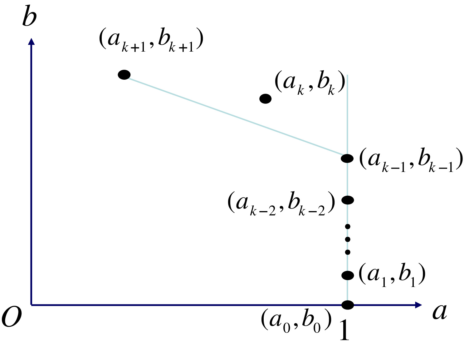
 (a0,b0),(a1,b1),…,(ak,bk),(ak+1,bk+1)
 (ak,bk)
 (ak−1,bk−1)
 (ak+1,bk+1)
 (ak−1,bk−1),(ak,bk),(ak+1,bk+1)

 k0=100
 δ=0.1
 ×
 ϵ¯i.i.d.(Tk0,n,δ)
 ∗
 ϵ¯(Tk0(0),n,δ)
 ϵ¯(T⌈νk0⌉(λ),n,δ)
 O(n−1)
 s=0.1
 δ=0.1
 ×
 ϵ¯i.i.d.(T⌈sn⌉,n,δ)
 ϵ¯(T⌈sνn⌉(λ),n,δ)
 O(n−1)
 ϵ¯(T⌈sn⌉(0),n,δ)
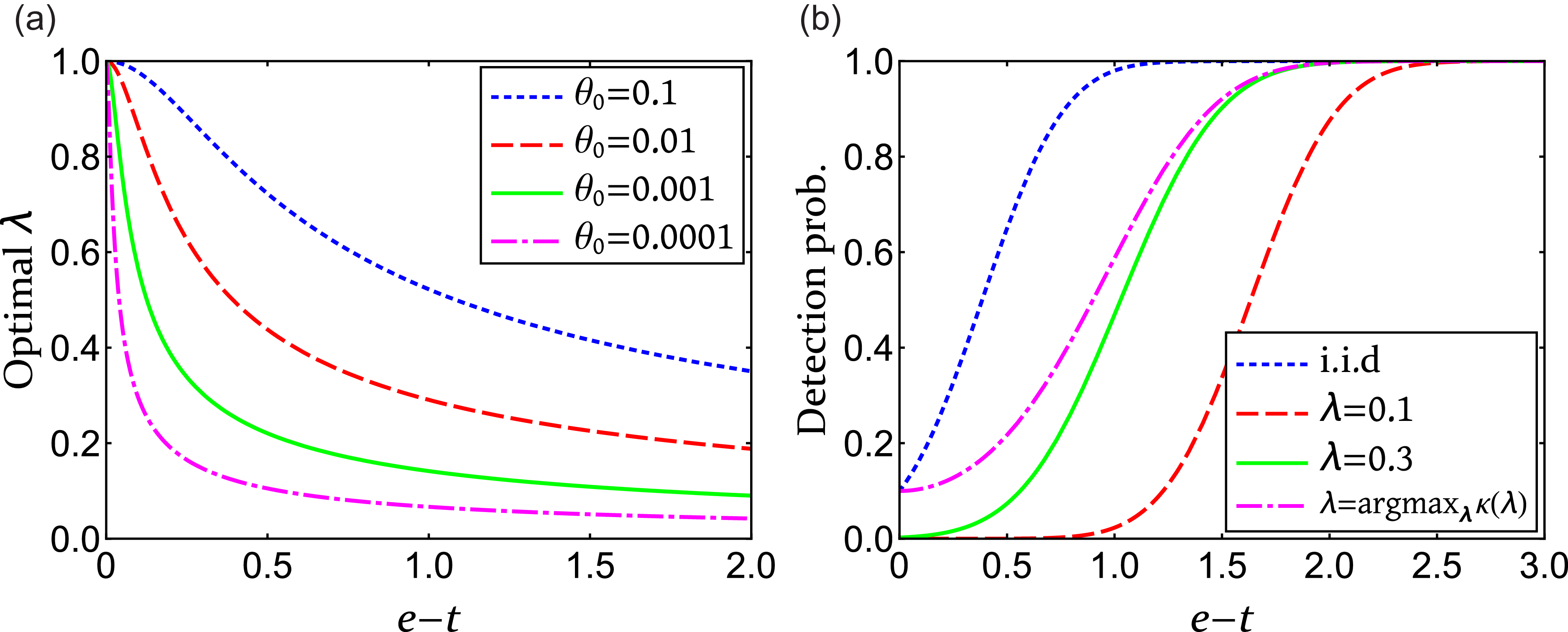
 argmaxλ∈(0,1)κ(λ)
 e−t
 θ0
 δ=0.1
 e−t
 θ0=0.1
 δ=0.1
 Φ
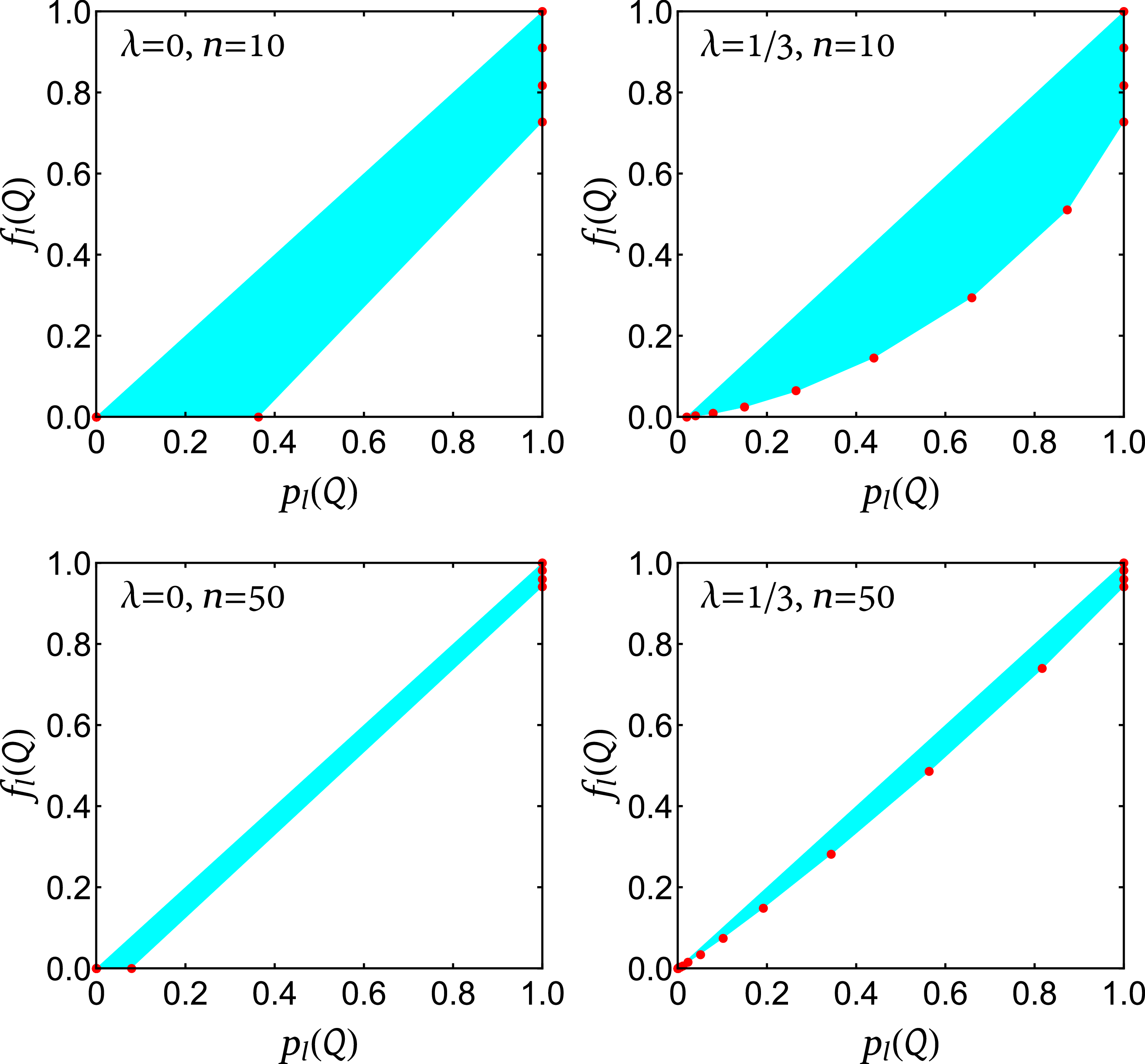
 Rl,n,λ
 (pl(Q),fl(Q))
 l=3
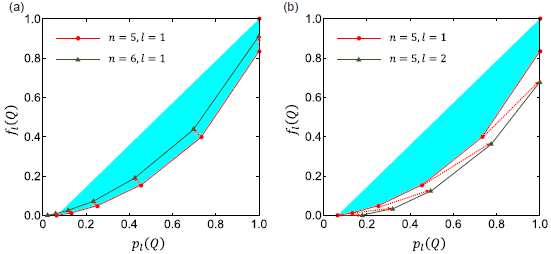
 Rl,n,λ
 Rl,n+1,λ
 n≥l+1
 Rl=1,n=5,λ=1/e
 Rl=1,n=6,λ=1/e
 Rl+1,n,λ
 Rl,n,λ
 n≥l+2
 Rl=1,n=5,λ=1/e
 Rl=2,n=5,λ=1/e


