




No CrossRef data available.
POWER FUNCTIONS AND ENVELOPES FOR UNIT ROOT TESTS
Published online by Cambridge University Press: 31 January 2003
Abstract
This paper studies power functions and envelopes for covariate augmented unit root tests. The power functions are calculated by integrating the characteristic function, allowing accurate evaluation of the power envelope and the power functions. Using the power functions, we study the selection among point optimal invariant unit root tests. An “optimal” point optimal test is proposed based on minimizing the integrated power difference. We find that when there are covariate effects, optimal tests use a local alternative where the power envelope has an approximate value of 0.75.We thank Pentti Saikkonen and two referees for helpful comments.
Information
- Type
- Research Article
- Information
- Copyright
- © 2003 Cambridge University Press
1. INTRODUCTION
Testing for the presence of unit roots is now a common practice in empirical macroeconomic and financial time series analysis. Although the unit root hypothesis has been tested in hundreds of time series, it is widely recognized that the discriminatory power of unit root tests is generally low. In addition, oftentimes practitioners do not know whether a trend is deterministic or stochastic, so it is necessary in empirical analysis to include deterministic terms in the model when estimating the hypothesized unit root parameter. This inclusion of “extra” deterministic components in the model reduces power from its already low level.
One of the mechanisms for increasing the power of unit root tests is related to point optimal testing procedures. The point optimal procedures, which are optimal only for a specific point alternative, can also be used to test for a unit root against more complex alternative hypotheses, although it is no longer optimal for alternatives at other points. Actually, a point optimal test based on an “appropriately chosen” value of the local parameter may have higher power than the conventional unit root tests. Because there is no uniformly most powerful test for the unit root hypotheses, a point optimal test using some plausible choice of local parameter value is a reasonable choice. Notice that a point optimal test will touch the power envelope at the corresponding local parameter value, so that there is an infinitely large class of tests, all of which are asymptotically admissible. A natural question to ask is: How should we choose an “optimal” point optimal test? We attempt to address this issue for a class of unit root tests in the current paper.
When ordinary least squares (OLS) is used (with no covariates), point optimal unit root tests have been studied by Elliott, Rothenberg, and Stock (1996) and Saikkonen and Luukkonen (1993). Elliott et al. (1996) show that the power of point optimal tests is not sensitive to the choice of the alternative so long as the point optimal test has a tangency between power 0.25 and 0.75. Elliott and Jansson (2000) propose point optimal invariant tests when covariate effects are estimated. We show that there are interesting differences that arise when using covariates so that the choice of a point optimal invariant test magnifies the familiar trade-off between alternatives close to the null and more distant alternatives. In this paper, we derive characteristic functions for covariate augmented unit root tests to accurately evaluate power envelopes and power functions for point optimal tests. Using power envelopes and power functions calculated from our characteristic functions, one can evaluate differences between point optimal tests and the envelope. This allows, perhaps, formulation of an “optimal” point optimal test.
The paper is organized as follows. In Section 2, we present the asymptotic power functions derived for invariant unit root tests developed by Elliott and Jansson (2000). Section 3 provides the characteristic functions for the power functions. Section 4 studies the selection of optimal point optimal unit root tests and reports new critical values used for a feasible version of the test. Section 5 concludes.
2. UNIT ROOT TESTS USING COVARIATES
Elliott and Jansson (2000) extend the covariate augmented unit root tests developed by Hansen (1995) to form point optimal tests invariant to deterministic terms. Because our focus is on the evaluation of the asymptotic power curves and envelopes, we take the asymptotic distributions as given and proceed with a strategy for evaluation.
Suppose that a time series yt can be decomposed into a deterministic component and a stochastic component, yt = dt + st, where dt = γ′zt, with zt a deterministic trend of known form. The stochastic part is represented as Δst = δst−1 + vt. We also assume δ = −(c/T). Suppose we wish to test the null hypothesis H0 : c = 0 versus Hc : c = c where c ≥ 0. The limiting distributions of the likelihood ratio test depend on the parameters c, c, and R2. The parameter c is the true value of the local parameter, whereas c is the hypothesized local parameter. The term R2 indicates the correlation between covariates and the quasi-difference of the local to unit root process (for a more detailed description of the unit root model with covariates, see Hansen, 1995; Elliott and Jansson, 2000). We consider three cases with emphasis on the two empirically relevant cases where a constant is estimated and a constant and trend are estimated. In particular, case 1 represents the distribution when there are no deterministic components estimated or when they are treated as known. In case 2, an intercept is included for both the covariates and the local to unit root process, whereas case 3 includes a constant and trend in both. Our cases 1, 2, and 3 correspond to the cases 1, 3, and 5, respectively, in Elliott and Jansson (2000). Denoting the limiting distributions corresponding to these three cases as LRj(c,c), j = 1, 2, 3, the limiting distributions are as follows:

where m1 = 1/(1 + c2/3 + c), W1c(r) is an Ornstein–Uhlenbeck process satisfying the stochastic differential equation

and W1cτ(s) = W1c(s) + (6s − 4)∫W1c(r) dr − (12s − 6)∫rW1c(r) dr, W1c = ∫W1c(r) dr.1
The parameters c and c are taken as positive, which is the opposite of Elliott and Jansson (2000) but the same as in Hansen (1995).
These limiting variates all have nonstandard distributions and are dependent on nuisance parameters. In practice, simulation methods are generally used to obtain approximations of these distributions. However, Nabeya and Tanaka (1990), Perron (1991), and Tanaka (1996) suggest a general approach for deriving the limiting distributions of OLS estimators for autoregressive parameters. We explore using similar methods for the covariate case in the next section.
3. CHARACTERISTIC FUNCTIONS
We find the characteristic functions of the limiting distributions and use them to find probabilities based on numerical integration. The probabilities are used to find critical values for a range of point alternatives that are then used to find the power envelope.
Evaluating the distributions using numerical integration has certain advantages over the traditional Monte Carlo based approximation. First, as documented in Nabeya and Tanaka (1990), accuracy is improved using numerical methods. For our purposes, this is important as we plan to use the derived power envelopes to find a class of optimal point optimal tests. Second, the computational time decreases substantially. This is important as we must evaluate and compare multiple power curves for point optimal tests.
The characteristic function of the random variable LRj(c,c) is defined as E(eiθLRj), and we denote this by φLRj(θ,c,c), j = 1, 2, 3. We give an expression for the characteristic function in the following theorem.2
Case 3 has a representation using sin λ and cos λ. However, this representation is several pages long, and we use the determinant representation to conserve space.
THEOREM 3.1.

Once we have obtained the characteristic function, calculating probabilities is based on numerical integration using Gurland's (1948) formula:

where Im is the imaginary part of the complex number.
Using the preceding formula, it is possible to calculate critical values for specific alternatives, which can then be used to obtain power envelopes and power functions for point optimal tests of the null hypothesis, H0 : c = 0. We compare these point optimal tests for several cases of the nuisance parameter R2 in the next section.
The power envelope was calculated by first finding critical values for the test indexed by c. That is, a critical value must be found for each alternative hypothesis and each value of the nuisance parameter R2 considered. After critical values are generated for each of the alternatives, the power is calculated by numerical integration with x = x0.05 so that P(LRj(0,c) ≤ x0.05) = 0.05. The power functions are denoted

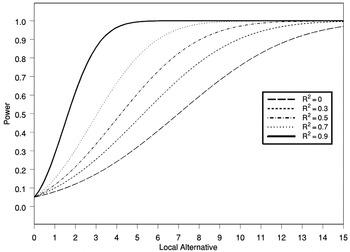
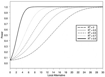
so that the power envelope is Π(c,c). For the numerical integration using characteristic functions, we found 2,500 values of the characteristic function and used a simple application of Simpson's rule to find the integral. The truncation of the integral was determined where the integrand consistently took a value of less than 10−20 in absolute value. The power envelopes for cases 2 and 3 appear in Figures 1 and 2 and correspond to Figures 1b and 1d in Elliott and Jansson (2000).

Case 2 envelopes.

Case 3 envelopes.
4. OPTIMAL POINT OPTIMAL UNIT ROOT TESTS
A point optimal test for H0 : c = 0 against Hc : c = c > 0 also naturally provides a test for alternative Hc : c > 0. Although, strictly speaking, such a test is only optimal for the specified alternative, a point optimal test with an appropriate selection of c can be nearly optimal in the sense that the power function is very close to the power envelope. Because there is no uniformly most powerful test, point optimal tests (against the alternative of c) are of interest and may provide a power gain relative to tests based simply on estimated autoregressive parameters.
Given the different behavior of tests based on different values of c, an obvious question is which of these tests has the best overall power properties. As suggested in King (1988), one possibility is to choose c so that the test is more powerful over certain ranges of the parameter space. A natural criterion for measuring the closeness of a power curve to the power envelope is the integral of the difference between a power curve and the power envelope, so that we may select the optimal point optimal test by minimizing the integrated power differences; i.e., we choose c by

Because the power envelope is above the power function Π(c,c), the difference between Π(c,c) and Π(c,c) is always nonnegative. Notice that criterion (4.1) is equivalent to maximizing the power function Π(c,c) integrated over c and the suggested criterion can be treated as an application of Cox and Hinkley (1974) to the unit root model.3
We thank an anonymous referee for pointing out this connection.
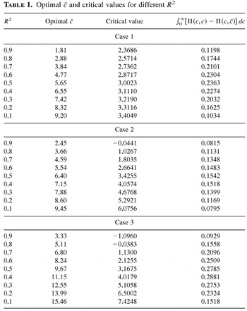
We apply the results developed in Section 3 to select an optimal point optimal test. The optimal choices of c (and thus the corresponding test) are found for representative R2 values. The integral is evaluated over the range from zero to 30 because the difference between the point optimal test and the envelope is negligible at this point. Point optimal tests indexed by c from .01 to 20 are considered because the integral is decreasing and then increasing in c. The integral is evaluated using Simpson's rule with 3,000 points, starting at 0.01 and 0.01 increments. The integral is evaluated for R2 = 0.1,…,0.9.
The output from searching for a class of optimal c is given in Table 1. First, we point out that the minimized integral of the difference between the power envelope and the power function of the point optimal test initially increases and eventually decreases as R2 increases. In fact, when R2 is nearly zero, the differences in the power envelope and the point optimal test are trivial. This is in agreement with the simulation evidence in Elliott et al. (1996) and the numerical evidence presented in Tanaka (1996). In addition, we found that the point optimal tests were tangent to the power envelope at approximately 0.75 regardless of the value of R2. For a wide range of R2 (except close to zero), these different choices of c are important. However, this is not of practical importance when R2 = 0 (or close to 0) as the difference in point optimal tests is very small.
Optimal c and critical values for different R2

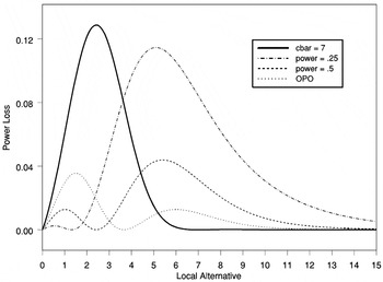
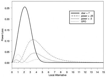
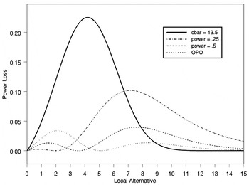
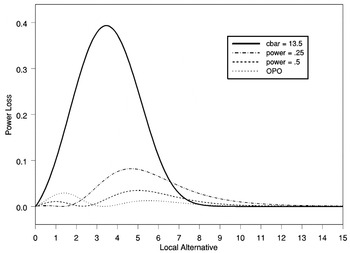
To illustrate the choice of tests, we plot the difference between the power envelope and several cases of point optimal invariant tests for the empirically relevant cases. Figure 3 presents the power differences for case 2 when R2 = 0.8. The optimal point optimal invariant test is denoted OPO and is compared with the point optimal invariant tests associated with power at 0.5 and 0.25. In addition, the case where c = 7 was suggested by Elliott and Jansson (2000) and is included for comparison.4
When c = 7, the point optimal test is tangent to the power envelope at 0.5 if there are no covariate effects. This is the same alternative used in Elliott et al. (1996).
For case 3, c = 13.5 is tangent to the power envelope at power = 0.5 when there is no covariate effect and a constant and trend are estimated.
See Figure 1 in Elliott et al. (1996) for a comparison of tests when R2 = 0.

Case 2: R2 = 0.8.

Case 2: R2 = 0.9.

Case 3: R2 = 0.8.

Case 3: R2 = 0.9.
5. CONCLUSION
We have developed expressions for characteristic functions for the limiting distribution of point optimal invariant tests for the unit root hypothesis using covariates. Using these characteristic functions, we are able to find power envelopes and power functions by numerical integration in the manner proposed in Nabeya and Tanaka (1990) and Perron (1991) for OLS based unit root tests.
Employing the power envelopes and power functions for point optimal tests, we find the “optimal” point optimal tests, in the sense that the integrated difference between the envelope and the point optimal tests is minimized. Remarkably, the tangency occurs where the power envelope takes a value of approximately 0.75 regardless of the magnitude of the covariate effect. The power gains from using these optimal tests (relative to the choice of alternative when there is no covariate effect) are greater as the covariate is more effective in explaining variation. The values of c and the critical values associated with the optimal point optimal invariant tests can be used in conjunction with Elliott and Jansson (2000).
Appendix
Proof of Theorem 3.1. The theorem follows Nabeya and Tanaka (1990) and Perron (1991) closely. We prove the result for case 2 because the other cases are similar. The proof is completed by finding E(eθLR2) and then replacing θ by iθ. First,

Condition on W1c so that we have

Following Perron (1991), use Girsanov's (1960) theorem to eliminate the ∫(W1c)2 terms, setting

The moment generating function becomes

Let X = W1β(1) and Y = ∫W1β. Then V = (X,Y)[top ] ∼ N(0,Σ) where

(see Tanaka, 1996, p. 234).
Then

Then

A simple change of variables gives us

After algebra, we have

Substituting iθ for θ and noting that β = iλ gives the result. █
References
REFERENCES
Cox, D.R. &
D.V. Hinkley
(1974)
Theoretical Statistics.
London:
Chapman and Hall.
Elliott, G. &
M. Jansson
(2000)
Testing for Unit Roots with Stationary Covariates.
Working paper,
University of California, San Diego.
Elliott, G.,
T.J. Rothenberg, &
J.H. Stock
(1996)
Efficient tests for an autoregressive unit root.
Econometrica
64,
813–836.CrossRefGoogle Scholar
Girsanov, I.V.
(1960)
On transforming a certain class of stochastic processes by absolutely
continuous substitution of measures.
Theory of Probability and Its Applications,
5,
285–301.CrossRefGoogle Scholar
Gurland, J.
(1948)
Inversion formulae for the distribution of ratios.
Annals of Mathematical Statistics
19,
228–237.CrossRefGoogle Scholar
Hansen, B.E.
(1995)
Rethinking the univariate approach to unit root testing.
Econometric Theory
11,
1148–1171.CrossRefGoogle Scholar
King, M.
(1983)
Testing for moving average regression disturbances.
Australian Journal of Statistics
25,
23–34.CrossRefGoogle Scholar
King, M.
(1988)
Towards a theory of point optimal testing.
Econometric Reviews
6,
169–218.Google Scholar
Nabeya, S. &
K. Tanaka
(1990)
Limiting powers of unit-root tests in time-series regression.
Journal of Econometrics
46,
246–271.CrossRefGoogle Scholar
Nelson, C.R. &
C. Plosser
(1982)
Trends and random walks in macroeconomic time series: Some evidence
and implications.
Journal of Monetary Economics
10,
139–162.CrossRefGoogle Scholar
Perron, P.
(1991)
A continuous time approximation to the unstable first-order
autoregressive process: The case without an intercept.
Econometrica
59,
211–236.CrossRefGoogle Scholar
Saikkonen, P. &
R. Luukkonen
(1993)
Point optimal tests for testing the order of differencing in ARIMA
models.
Econometric Theory
9,
343–362.CrossRefGoogle Scholar
Tanaka, K.
(1996)
Time Series Analysis.
New York:
Wiley.
Case 2 envelopes.
Case 3 envelopes.
Optimal c and critical values for different R2
Case 2: R2 = 0.8.
Case 2: R2 = 0.9.
Case 3: R2 = 0.8.
Case 3: R2 = 0.9.
 You have
Access
- 12
- Cited by