

1. INTRODUCTION
Decision theorists have suggested that it is sometimes appropriate to represent the value of certain options as intervals of real numbers.Footnote 1 In this note I show that doing so is incompatible with some deeply held intuitions about rational choice.
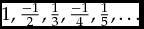
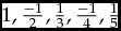
Claims about interval values can be motivated in different ways.Footnote 2 Here I focus on Lauwers and Vallentyne's (Reference Lauwers and Vallentyne2016) recent suggestion to assign interval values to some Pasadena-style gambles.Footnote 3 The original version of the Pasadena gamble can be formulated as follows:Footnote 4 You toss a fair coin n times until it lands heads up for the first time; if n is odd you win (2n)/n units of value, but if n is even you have to pay (2n)/n. It is tempting to claim that the expected value of the Pasadena gamble is  $\frac{1}{2} \cdot \frac{2}{1} - \frac{1}{4} \cdot \frac{4}{2} + \frac{1}{8} \cdot \frac{8}{3} - \frac{1}{{16}} \cdot \frac{{16}}{4} + \frac{1}{{32}} \cdot \frac{{32}}{5} \ldots = 1 - \frac{1}{2} + \frac{1}{3} - \frac{1}{4} + \frac{1}{5} \ldots = \mathop \sum_n^{} \frac{{{{( { - 1} )}^{n - 1}}}}{n} $. However, according to the Riemann Rearrangement Theorem the sum of these terms, known as the alternating harmonic series, depends on the order in which they are summed up. If the terms are added together in the manner indicated above the sum is ln 2, but by rearranging the order we can make the sum converge to any real number, including −∞ and +∞.Footnote 5 Decision theorists have been puzzled by this mathematical fact. What is the value of something if the sum of its parts depends on the order in which they are added up? Easwaran (Reference Easwaran2008) famously introduces a distinction between weak and strong expectations.Footnote 6 The weak expected value of the Pasadena gamble is ln 2, which Easwaran takes to be the value that should guide our choices. However, as Easwaran himself is aware, some slightly modified versions of the Pasadena gamble have neither strong nor weak expectations.Footnote 7 Consider, for instance, the oscillating gamble (see Table 1) introduced by Lauwers and Vallentyne (Reference Lauwers and Vallentyne2016: 392).
The Oscillating Gamble.

In the oscillating gamble the first term in the series of possible outcomes is positive, the next two are negative, the next four are positive, and the next eight are negative, and so on. By multiplying the probability of each state with the value of the corresponding outcome we get  $1 - \frac{1}{2} - \frac{1}{3} + \frac{1}{4} + \frac{1}{5} + \frac{1}{6} + \frac{1}{7} - \frac{1}{8}$. . . . As we keep adding up these terms, the sum is sometimes close to 0 and sometimes close to 1, but it oscillates up and down no matter how long we keep adding the terms together. As explained by Lauwers and Vallentyne, this ensures that the oscillating gamble has no weak expected value.Footnote 8 Their proposal is that we should think of the oscillating gamble as having an “interval value”. On their view, the value of the oscillating gamble is the interval [0,1]. This interval is no mere approximation of some yet unknown point value. The entire interval between 0 and 1, including its endpoints, represents the value of the gamble.
Although Lauwers and Vallentyne do not make any claim about rational choice themselves (but rather about value), nearly all decision theorists would agree that evaluations of options that have nothing to say about how decision makers should choose are at best incomplete. In the next section we state a simple yet powerful impossibility result, which is applicable not just to interval values assigned to Pasadena-style gambles but to every interval value no matter how it is derived.
2. AN IMPOSSIBILITY RESULT
If we believe that the value of the oscillating gamble is [0,1], then it is appropriate to ask how a rational agent should choose if offered a choice between something worth [0,1] and some other option worth, say, 1/3 or 1/2 units of value. Lauwers and Vallentyne correctly point out that if the minimum value of some interval [a,b] exceeds the maximum of some other interval [c,d], then [a,b] is better than [c,d], meaning that it is not rationally permissible to choose the latter option if the former is available.Footnote 9 However, this observation does not cover choices between overlapping intervals (e.g. a choice between [0,5] and [2,3]) or between intervals and real-valued points within an interval (e.g. a choice between [0,1] and 0.5). The claim that the oscillating gamble is worth [0,1] is, arguably, hard to evaluate until we know how to choose among all possible combinations of options.
In what follows we will consider some general conditions a decision theory for interval values ought to satisfy. To start with, it is reasonable to assume that interval values cannot be reduced to point values: For every interval value [x,y], with x≠ y, there is no real-valued point a such that [x,y] ~ a, where ~ means that the two options are equally valuable. If the interval value [x,y] turned out to be worth exactly as much as some real-valued point a, then there would be no need for interval values in decision theory. Suppose, for instance, that the interval value of the oscillating gamble, [0,1], is worth exactly 0.5. The value of the oscillating gamble would then simply be that particular real number. This would make the interval value redundant. In the formal impossibility result stated at the end of this section we invoke the following, somewhat stronger version of this idea, in which a > b means that a is more valuable than b.
Local Incomparability. For every interval value [x,y], where x≠ y, there exist at least two real-valued points a, b such that a > b and:
(i) ¬([x,y] > a) and ¬([x,y] ~ a) and ¬([x,y] < a)
(ii) ¬([x,y] > b) and ¬([x,y] ~ b) and ¬([x,y] < b)
The motivation for this condition can be broken down into two parts. First, although some point-values are better or worse than some interval values (e.g. a point value that exceeds the maximum of the interval), interval values would be of little interest unless there exists at least one point that is neither better, worse, nor equally good as the interval. As noted above, interval values must not be reducible to point values.Footnote 10 Second, if there is one such point, there has to be two. Why? Because otherwise, for every other point b located arbitrary close to a, the point b would have to be better, worse or equally good as the interval. We can exclude the possibility that b is equally good as the interval, because then the value of the interval could obviously be reduced to a point-value, which we are not willing to accept, as noted above. We are thus left with the possibility that every point b < a is worse than the interval while every b > a is better, which leads to further trouble. To see this, we assume that a rational and fully informed agent is indifferent between options just in case they are of equal value. We then apply Savage's well-known definition of indifference:
If the person really does regard [two options] as equivalent, that is, if he is indifferent between them, then, if [one of the options] were modified by attaching an arbitrarily small bonus to its consequences in every state, the person's decision would presumably be for whichever act was thus modified. (Savage Reference Savage1954: 17)
Savage's definition entails that if there is only one point a of the type described in Local Incomparability, then the agent would, according to this widely accepted definition of indifference, be indifferent between a and [x,y], because every slightly improved version of a (including b) would be preferred to [x,y]. So [x,y] ~ a, which contradicts our initial assumption. The upshot is that the distinction between indifference and incomparability requires the existence of at least two points that are neither better, worse, or equally good as something else. Incomparability cannot be fully local.
The remaining conditions should be familiar to the reader.Footnote 11 Let S denote the set of feasible options and let C(S) be a subset of rationally permissible options in S. Our second condition states that it is not permissible to choose an option if some better option is available:
Better. For all a, b ∈ S, if a > b then b∉ C(S)
The next condition holds that at least one option in each choice problem is rationally permissible.
No Dilemmas. For every S, there is some a such that a ∈ C(S).
The fourth and final condition is designed to exclude the possibility that one of two incomparable options is rationally permissible while the other is not. This is probably the most controversial condition. I will discuss it at length in the next section:
Choice Parity. For all a, b ∈ S, if ¬(a > b) and ¬(a ~ b) and ¬(b < a), then a ∈ C(a) iff C(b).
It can be easily verified that at least one of the four conditions stated here has to be rejected:
Observation. Local Incomparability, Better, No Dilemmas and Choice Parity are logically inconsistent.
Proof. We assume that any set of values is a feasible set and that options can be identified with their values.Footnote 12 Consider the interval [x,y]. Local Incomparability guarantees the existence of points a and b, with a > b such that [x,y] is incomparable with both a and b. (Formally: (i) ¬([x,y] > a) and ¬([x,y] ~ a) and ¬([x,y] < a) and (ii) ¬([x,y] > b) and ¬([x,y] ~ b) and ¬([x,y] < b).) Let S = {a, b, [x, y]} be a set of feasible options. Because a > b, Better entails that b∉ C(S). Hence, No Dilemmas entails that a ∈ C(S) or [x, y] ∈ C(S) . If a ∈ C(S) then Choice Parity entails that [x, y] ∈ C(S), and by applying Choice Parity again we find that b ∈ C(S), which contradicts the conclusion (above) that b∉ C(S). The second case, [x, y] ∈ C(S), is analgous to the first.
3. DISCUSSION
Should we feel worried by this impossibility result? Although it is not very exciting from a technical point of view it makes the decision theorist's worries about interval values explicit. Lauwers and Vallentyne, as well as other advocates of interval values, have to reject at least one of the four conditions.
Vallentyne believes that Choice Parity is too strong.Footnote 13 In his view, we should conclude that sometimes only one of two incomparable options is permissible. Imagine, for instance, that we are offered three options worth [0,1], 0.49 and 0.51 units of value, and conclude that [0,1] and 0.49, as well as [0,1] and 0.51, are incomparable. Would it then be reasonable to maintain that [0,1] is permissible if 0.49 is permissible? The fact that we can choose 0.51, which is better than 0.49, might be taken to indicate that although [0,1] and 0.49 are incomparable, [0,1] but not 0.49 is permissible. If so, Choice Parity is false.
I agree that this manoeuvre would avoid the inconsistency outlined above. But what is the reason for accepting all this, apart from the fact that it solves the problem? Perhaps it could be argued that one of the options in the example has a property the other lacks.Footnote 14 The option worth 0.49 has the property of being less valuable than some feasible option (viz. 0.51); the interval [0.1] does not have that property. Of course, we all agree that this makes it rationally impermissible to choose 0.49 whenever 0.51 is available, as stipulated by Better. But why would this be a reason for rejecting Choice Parity? The latter condition merely asserts that if [0,1] is rationally permissible then so is 0.49, and vice versa. What is missing here is a reason for thinking that [0,1] would be rationally permissible when 0.51 and 0.49 are available.Footnote 15
It is also worth pointing out that the refutation of Choice Parity leads to another problem. If the mere presence of a third option affects the permissibility of the two other options, then this violates Sen's principle beta. (If x and y are rationally permissible options in A, and A ⊆ B, then x is a rationally permissible option in B iff y is a rationally permissible option in B.) Principle beta is not accepted by everyone, but my view is that it is not reasonable to give up this principle just to make room for interval values.Footnote 16 If we let pairwise comparisons between two options depend on the presence of a third option, it seems to me that the characterization of the normatively relevant properties of those options may have been incomplete.Footnote 17
A more promising response to the impossibility result could be to make room for genuine dilemmas in decision theory, that is, reject No Dilemmas. Although it seems implausible to claim that all options may be rationally impermissible, one can make roughly the same point by questioning the assumption that rational permissibility is a binary property. Perhaps it is neither fully permissible nor fully impermissible to choose [0,1] in a choice between that option and 0.51. All things considered, each option might be somewhat impermissible and somewhat permissible. Claims about rationality need not be black or white. Perhaps rational permissibility comes in different shades of grey.Footnote 18 On such a nonbinary view, it is not implausible to think that it is somewhat less impermissible, but not fully permissible, to choose 0.51 instead of [0,1].
However, even if we accept this somewhat exotic idea, the impossibility result would still go through as long as we can construct a case in which one option is strictly better (in the binary sense) than another and both these options are permissible to the same degree when compared to some third option. Note that this is true irrespective of which (minimally plausible) ordinal or cardinal representation of degrees of permissibility we prefer.Footnote 19
To reject Better is, in my opinion, out of the question. If one option is better than another in the traditional, binary sense, then it is not rationally permissible to choose the second option, period.
Although the remarks in this paper are primarily motivated by Lauwers and Vallentyne's analysis of the oscillating gamble, it is worth noting that the scope of the impossibility result is broader. For instance, authors who believe that options can be of ‘roughly equal’ value (Parfit Reference Parfit1984) or be ‘on a par’ (Chang Reference Chang2002) also have reason to worry about this result. The Local Incomparability condition seems to be equally applicable to options that are roughly equal or on a par, as are the three other ones. If some options are roughly equal or on a par, then there are at least two local point-values that are neither better, worse or equally good as options to which they stand in that relation to. Neither rough equality nor parity can be fully local phenomena.
It is also worth keeping in mind that the probabilistic nature of the Pasadena-style choices discussed by Lauwers and Vallentyne is not essential for their appeal to interval values. Pasadena-style problems can arise in nonprobabilistic contexts; see Peterson (Reference Peterson2013a).Footnote 20
All this suggests that the scope of the impossibility theorem stated in this paper is fairly large. It applies to a wide range of gambles and nonprobabilistic choice situations and it is not the principle of maximizing expected value that is at stake in these problems, but rather the idea that the value of the whole is equal to some interval of real numbers. We may, therefore, wish to reject the proposal that sometimes the value of an option is an interval of real numbers.
ACKNOWLEDGEMENTS
I would like to thank Peter Vallentyne and two anonymous reviewers for extremely helpful comments on earlier versions of this paper.