



1 Introduction
Let M denote the interior of a compact smooth manifold with boundary
 $\overline {M}$
, and let
 $\overline {g}$
be a nondegenerate smooth metric on
 $\overline {M}$
. Let
 $r\in C^\infty (\overline {M})$
with
 $r\geq 0$
on M,
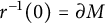 ${r^{-1}(0)=\partial M}$
. Consider the metric g on M given by
 $g=r^{-2}\overline {g}$
. Then, we call g a conformally compact metric and
 $(M,g)$
a conformally compact manifold. In addition, if
 $(M,g)$
satisfies
 $|dr|_{\overline {g}}=1$
on
 $\partial M$
, it can be shown in [Reference Mazzeo24] that this condition is equivalent to the sectional curvature uniformly tends to
 $-1$
as we approach the boundary
 $\partial M$
. When this additional condition holds, we say that the conformally compact manifold
 $(M,g)$
is asymptotically hyperbolic.
Suppose that M and N are Riemannian manifolds of dimensions m and
 $n,$
respectively, and their Riemannian metrics are
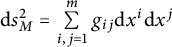 $\mathrm {d} s^2_{M}=\sum \limits _{i,j=1}^{m}g_{ij}\mathrm {d} x^i\mathrm {d} x^j$
and
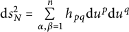 $\mathrm {d} s^2_{N}=\sum \limits _{\alpha ,\beta =1}^{n}h_{pq}\mathrm {d} u^p\mathrm {d} u^q$
, respectively. Then, the energy density function of a
 $C^1$
map
 ${u: M \rightarrow N}$
is defined by
 $$\begin{align*}e\left(u\right)=\frac{1}{2}g^{ij}\frac{\partial u^p}{\partial x^i}\frac{\partial u^q}{\partial x^j}h_{pq},\end{align*}$$
and the total energy of u is given by
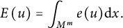 $$\begin{align*}E\left(u\right)=\int_{M^m} e(u)\mathrm{d} x.\end{align*}$$
The harmonic map equation from M into N, which is the Euler–Lagrange equation for critical points of the total energy functional, can be written as
 $$\begin{align*}\tau(u)^s=\Delta_{M} u^s+g^{ij}{\Gamma}_{pq}^s\frac{\partial u^p}{\partial x^j}\frac{\partial u^q}{\partial x^i}=0, s=1,\ldots ,n, \end{align*}$$
where
 ${\Gamma }_{pq}^s$
are the Christoffel symbols of N.
The model example for asymptotically hyperbolic manifolds is Poincaré model for hyperbolic space
 $\mathbb {H}^m$
given by the unit ball
 ${B}^m$
with metric
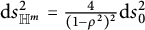 $\mathrm {d}s_{\mathbb {H}^m}^2 = \frac {4}{(1-\rho ^2)^2} \mathrm {d}s_0^2$
. Here,
 $\rho $
denotes the Euclidean distance measured from the origin, and
 $\mathrm {d}s_0^2$
stands for the standard Euclidean metric. Under this equivalence relation, a map from the
 $(m - 1)$
-dimensional sphere
 $\mathbb {S}^{m - 1}$
to the
 $(n - 1)$
-dimensional sphere
 $\mathbb {S}^{n - 1}$
can be interpreted as a map from the boundary at infinity of
 $\mathbb {H}^m$
to the boundary at infinity of
 $\mathbb {H}^n$
. Schoen [Reference Schoen27] proposed a conjecture: For every quasiconformal mapping
 $f: \mathbb {S}^1 \to \mathbb {S}^1$
, there exists a unique harmonic and quasiconformal extension
 $\mathcal {H}(f): \mathbb {H}^2 \to \mathbb {H}^2$
. Li and Wang [Reference Li and Wang18] extended this conjecture to the case where
 $m=n \geq 2$
.
The results of uniqueness, existence, and regularity properties for the Dirichlet problem at infinity for proper harmonic maps between hyperbolic spaces were obtained by Li and Tam [Reference Li and Tam15–Reference Li and Tam17] when the harmonic map is
 $C^1$
up to boundary. In their work [Reference Li and Tam17], they investigated the boundary regularity of these harmonic maps and posed some thought-provoking questions. Specifically, they wondered if the singularities of these harmonic maps could be understood by showing that near the boundary, the harmonic map must have an expansion similar to those in the complex Monge–Ampère equation [Reference Lee and Melrose12] and the Bergman Laplacian [Reference Graham10]. Donnelly [Reference Donnelly4, Reference Donnelly5] generalized a portion of their findings to any rank one symmetric spaces. When the boundary map is a quasiconformal map, Li, Tam, and Wang [Reference Li and Tam17, Reference Li and Wang18] established the uniqueness and Lemm and Markovic [Reference Lemm and Marković13, Reference Marković22, Reference Marković23] proved existence using heat flow theorem in [Reference Wang28]. Benoist and Hulin [Reference Benoist and Hulin2] completed the proof of the Schoen–Li–Wang conjecture when both the domain manifold and the target manifold are symmetric spaces of rank one. The complex case was studied by Donanelly [Reference Donnelly6] Li and Ni [Reference Li and Ni19] Li and Simon [Reference Li and Simon20], etc. When the boundary map is smooth and has nowhere vanishing energy density, Chen, Li, and Luo provide an asymptotic expansion formula for the harmonic map between balls in Berman metrics in [Reference Chen, Li and Luo3], so they obtained the optimal regularity of harmonic maps in the case of complex spaces.
There have also been several relevant works on harmonic maps between asymptotically hyperbolic spaces. Leung [Reference Leung14] employed the heat flow method to demonstrate the existence of harmonic maps between asymptotically hyperbolic conformally compact manifolds. Regarding boundary regularity, Economakis proved that any
 $C^{1,1}$
local harmonic map whose boundary map is smooth and has nowhere vanishing energy density admits a polyhomogeneous expansion at the boundary in [Reference Economakis8]. Economakis adopted an approach that is purely microlocal, as can be seen in the references [Reference Lee and Melrose12, Reference Mazzeo25, Reference Mazzeo26]. Donnelly [Reference Donnelly7] proved existence and uniqueness for asymptotic Dirchlet problems for harmonic maps from Hadamard manifolds to complete simply connected manifolds with nonpositive sectional curvature. Kim and Lee [Reference Kim and Lee11] proved the existence of nonconstant bounded harmonic maps on a Cartan–Hadamard manifold of pinched negative curvature by solving the asymptotic Dirichlet problem. Akutagawa and Matsumoto [Reference Akutagawa and Matsumoto1] generalized the result of Li and Tam [Reference Li and Tam16], they proved an existence theorem for harmonic maps with
 $C^1$
boundary conditions between asymptotically hyperbolic manifolds. For other studies on harmonic maps between asymptotically hyperbolic spaces, see [Reference Fotiadis9, Reference Mazzeo24].
Compared with the above works, this article has two advantages. First, it improves the boundary regularity in Li and Tam [Reference Li and Tam17] and achieves the optimal boundary regularity. Second, it reduces the assumption of [Reference Economakis8] for harmonic maps between asymptotically hyperbolic spaces to
 $C^1$
up to the boundary, and obtains an expansion of harmonic maps between a class of asymptotically hyperbolic spaces. Moreover, in the Poincaré disk model, this expansion is global. In the case where both M and N are hyperbolic spaces, according to the asymptotic expansion obtained in this article, it is easy to see that the coefficient of the first power of the logarithm, which has an impact on the regularity, can be completely determined by the boundary map. Moreover, the specific expression of this coefficient can be calculated.
Let
 $\mathbb {H}^m$
and
 $\mathbb {H}^n$
be hyperbolic spaces of dimensions m and n, respectively. The hyperbolic space
 $\mathbb {H}^m$
is identified with
 $B^m=\{x\in \mathbb {R}^m | |x|<1 \}$
with the Poincaré metric given by
 $$\begin{align*}g_{\mathbb{H}^m}=\frac{4(dx^1 \otimes dx^1 + \cdots + dx^m \otimes dx^m)}{(1-\rho^2)^2}, \end{align*}$$
where
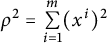 $\rho ^2=\sum \limits _{i=1}^m(x^i)^2$
. Under this identification, the idea boundary of
 $\mathbb {H}^m$
can be viewed as
 $\mathbb {S}^{m-1}$
. Similarly, we identify
 $\mathbb {H}^n$
with the unit ball
 $B^n$
in
 $\mathbb {R}^n$
with Poincaré metric given by
 $$\begin{align*}g_{\mathbb{H}^n}=\frac{4(du^1 \otimes du^1 + \cdots + du^n \otimes du^n)}{(1-|u|^2)^2}. \end{align*}$$
Also, the idea boundary of
 $\mathbb {H}^n$
is identified with
 $\mathbb {S}^{n-1}$
. In terms of these coordinates, the tension field of a map
 $u:\mathbb {H}^m\rightarrow \mathbb {H}^n$
is given by
 $$ \begin{align} \begin{aligned} \tau_0(u)^p=&\frac{(1-\rho^2)^2}{4}\Delta_0u^p+\sum\limits_{i=1}^m\frac{(m-2)(1-\rho^2)}{2}x^i\frac{\partial u^p}{\partial x^i}\\ &+\frac{(1-\rho^2)^2}{2(1-|u|^2)}(2 \langle u , \nabla_0 u \rangle \nabla_0u^p-\langle \nabla_0 u, \nabla_0 u \rangle u^p), p=1,\ldots,n, \end{aligned} \end{align} $$
where
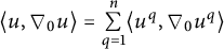 $\langle u , \nabla _0 u\rangle =\sum \limits _{q=1}^n \langle u^q , \nabla _0 u^q \rangle $
and
 $\langle \nabla _0 u, \nabla _0 u \rangle =\sum \limits _{q=1}^n\langle \nabla _0 u^q, \nabla _0 u^q \rangle $
. The notation
 $\Delta _0$
denotes the Euclidean Laplacian and
 $\nabla _0$
denotes the Euclidean gradient.
 $\langle \cdot , \cdot \rangle $
represents the inner product of two n-dimensional vectors.
We assume that M is a class of asymptotically hyperbolic spaces. In the Poincaré disk model
 $B^m=\{x\in \mathbb {R}^m | |x|<1 \}$
, it has a metric
 $$ \begin{align} \begin{aligned} g_M=\frac{4(dx^1 \otimes dx^1 + \cdots + dx^m \otimes dx^m)}{(1-\rho^2)^2}+h_M(x), \end{aligned} \end{align} $$
where
 $\rho =|x|$
. The term
 $h_M(x)$
is a symmetric 2-tensor, which serves as the perturbation term. It has the expansion
 $$ \begin{align*} \begin{aligned} h_M=\sum\limits_{i,j}^mh_{ij}dx^i\otimes dx^j. \end{aligned} \end{align*} $$
When expressed as a function of the variables
 $(\rho ,\theta )$
,
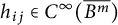 $h_{ij}\in C^\infty (\overline {B^m})$
adheres to a decay condition. Precisely, for any non-negative integer
 $s, k$
, the following relation holds:
 $$ \begin{align*} \begin{aligned} |\nabla^k_{\rho}\nabla^s_\theta h_{ij}|=O((1-|\rho|^2)^{a-k}), \rho \to 1^-, a>-1. \end{aligned} \end{align*} $$
Similarly, we assume that N is an asymptotically hyperbolic space and we identify N with the unit ball
 $B^n$
in
 $\mathbb {R}^n$
with Poincaré metric given by
 $$ \begin{align} \begin{aligned} g_N=\frac{4(du^1 \otimes du^1 + \cdots + du^n \otimes du^n)}{(1-|u|^2)^2}+h_N(x), \end{aligned} \end{align} $$
where
 $h_N(x)$
is a symmetric 2-tensor (i.e., the perturbation term) and has the expansion
 $$ \begin{align*} \begin{aligned} h_N=\sum\limits_{i,j}^n\overline{h}_{ij}du^i\otimes du^j. \end{aligned} \end{align*} $$
When expressed as a function of the variables
 $(\rho ,\theta )$
,
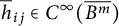 $\overline {h}_{ij}\in C^\infty (\overline {B^m})$
satisfies the decay condition: for any non-negative integer
 $s, k$
,
 $$ \begin{align*} \begin{aligned} |\nabla^k_{\rho}\nabla^s_\theta \overline{h}_{ij}|=O((1-|u|^2)^{b-k}), \rho \to 1^-, b>-1. \end{aligned} \end{align*} $$
In terms of these coordinates, the tension field of a map
 $u:M\rightarrow N$
is given by
 $$ \begin{align} \begin{aligned} \tau(u)^p =&\sum\limits_{i,j=1}^m(\frac{(1-\rho^2)^2}{4}\delta_{ij}+O((1-\rho^2)^{4+a}))\frac{\partial^2 u^p}{\partial x^i\partial x^j}\\ &+\sum\limits_{i=1}^m\frac{(m-2)}{2}((1-\rho^2)+O((1-\rho^2)^{3+a})x^i\frac{\partial u^p}{\partial x^i}\\ &+\frac{(1-\rho^2)^2+O((1-\rho^2)^{4+a})}{2}(\frac{1}{1-|u|^2}+O((1-|u|^2)^{b+1}))\\ &\times(2 \langle u , \nabla_0 u \rangle \nabla_0u^p-\langle \nabla_0 u, \nabla_0 u \rangle u^p), p=1,\ldots,n. \end{aligned} \end{align} $$
Let
 $\phi _0: \mathbb {S}^{m-1}\rightarrow \mathbb {S}^{n-1}$
. The Dirichlet boundary value problem for a proper harmonic map is given by
 $$ \begin{align} \begin{aligned} \tau(u)&=0 \text{ in } B^m \\ u&=\phi_0 \text{ on } \partial B^m. \end{aligned} \end{align} $$
The main purpose of this article is to study optimal boundary regularity for proper harmonic maps between asymptotically hyperbolic spaces similar to those in [Reference Li, Nguyen and Xiong21]. The main theorem is as follows.
Theorem 1.1 Let M and N be asymptotically hyperbolic spaces with metrics (1.2) and (1.3), respectively, in the Poincaré disk model. Let u be a harmonic map from M to N so that
 $u\in C^1$
as a map from
 $\overline {B^m}$
to
 $\overline {B^n}$
. Suppose that the boundary map
 $\phi _0$
of u, when restricted to
 $\mathbb {S}^{m-1}$
, is in
 $C^{\infty }(\mathbb {S}^{m-1}, \mathbb {S}^{n-1})$
, and has nowhere-vanishing energy density with respect to the standard metrics. Then,
 $u\in C^{m,\alpha }(\overline {B^m},\overline {B^n})$
for all
 $0<\alpha <1$
. Moreover, the solution u of (1.5) has the following asymptotic expansion:
 $$ \begin{align} \begin{aligned} u(x)\sim \phi_0+\sum\limits_{k=1}^{\infty}\overline{\phi}_k(x)d^k+\sum\limits_{k=m+1}^{\infty}\sum\limits_{l=1}^{[\frac{k-1}{m}]} \overline{\psi}_{k,l}(x)d^k(\log (-d))^l, \end{aligned} \end{align} $$
where
 $\overline {\phi }_k$
and
 $\overline {\psi }_{k,l}\in C^\infty (\overline {B^m};\overline {B^n})$
,
 $d(x)=|x|-1$
.
Remark 1.2 Here, (1.6) is understood in the sense that, for every
 ${m_0\geq m+1}$
and with
 $w_{m_0}=\phi _0+\sum \limits _{k=1}^{m_0}\overline {\phi }_k(x)d^k+\sum \limits _{k=1}^{m_0}\sum \limits _{l=m+1}^{[\frac {k-1}{m}]} \overline {\psi }_{k,l}(x)d^k(\log (-d))^l$
, we have
 $|\nabla ^j_\rho \nabla ^s_\theta (u-w_{m_0})|=O(d^{m_0+1-j-\varepsilon })$
, for any
 $\varepsilon>0$
and non-negative integers
 $s, j$
.
Remark 1.3
 $|\phi _0|^2=1$
on
 $\mathbb {S}^{m-1}$
. Differentiating with respect to
 $\theta _j\in \mathbb {S}^{m-1}$
, we can get
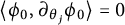 $\langle \phi _0 , \partial _{\theta _j} \phi _0 \rangle =0$
on
 $\mathbb {S}^{m-1}$
,
 $j=1,\ldots , m-1$
.
The main challenge is that since harmonic map is a system of semi-linear equations, the comparison principle is not applicable in some cases. To address this, we use the method of Fourier series expansion for functions on the Poincaré ball model to prove that taking the derivative in the tangential direction has little effect on the boundary regularity (see Lemma 3.2). For the mixed terms of different components in the system of equations, we regard it as a whole for estimation.
The organization of this article is as follows. In Section 2, we construct a good approximate solution
 $\overline {w}$
. This approximate solution has the form
 $\overline {w}=\phi _0+\sum \limits _{k=1}^{m} \overline {\phi }_k(\rho -1)^k+\overline {\psi }_{m+1,1}(\rho -1)^{m+1} \log (1-\rho )$
, where
 $\overline {\phi }_k(\theta ), \overline {\psi }_{m+1,1}(\theta )\in C^\infty (\mathbb {S}^{m-1};\mathbb {S}^{n-1})$
and
 $\tau (\overline {w})=O((1-\rho )^{m+2}\log (1-\rho ))$
. In Section 3, we extend methods and conclusions of [Reference Li and Tam16] to the harmonic maps between asymptotically hyperbolic spaces. Moreover, by using the method of Fourier series expansion, we prove that taking derivatives in the tangential direction has little effect on the boundary regularity. In Section 4, we prove Theorem 1.1 by using the method of solving ordinary differential equations.
2 The coefficient functions
 $\phi _0,\ldots , \phi _m, \psi _{m+1,1}$

In this section, we mainly prove Theorem 2.1. The coefficients
 $\phi _0,\ldots , \phi _m, \psi _{m+1,1}$
are completely determined by
 $\phi _0$
. Based on the expressions of
 $\tau _0$
and
 $\tau $
in (1.1) and (1.4), we can make a modification to
 $\phi _0,\ldots , \phi _m, \psi _{m+1,1}$
in Theorem 2.8. As a result, we obtain
 $\overline {\phi }_1, \overline {\phi }_2,\ldots , \overline {\phi }_m, \overline {\psi }_{m+1,1}$
in
 $C^{\infty }(\mathbb {S}^{m-1}, \mathbb {S}^{n-1})$
and the vector function
 $\overline {w}=\phi _0+\sum \limits _{k=1}^{m} \overline {\phi }_kd^k+\overline {\psi }_{m+1,1}d^{m+1} \log (-d), d=\rho -1$
such that
 $|\tau (\overline {w})|=O(d^{m+2}\log (-d))$
. In fact, according to the proof of Theorem 2.1, for any
 $m_0\geq 0$
, we can obtain
 $\overline {w}_{m_0}$
such that
 $|\tau (\overline {w}_{m_0})|=O(d^{m_0+1}\log (-d))$
. However,
 $\overline {\phi }_{m+1}$
cannot be completely determined by
 $\phi _0$
. We temporarily set the value of
 $\overline {\phi }_{m+1}$
to zero, and Lemma 4.2 will make the correction.
Theorem 2.1 Let
 $\phi _0 \in C^{\infty }(\mathbb {S}^{m-1}, \mathbb {S}^{n-1})$
be a boundary map with nowhere-vanishing energy density. There exist vector functions
 $\phi _1,\ldots , \phi _m, \psi _{m+1,1}$
in
 $C^{\infty }(\mathbb {S}^{m-1}, \mathbb {S}^{n-1})$
such that the vector function
 $$ \begin{align*} \begin{aligned} w=\sum\limits_{k=0}^{m} \phi_kd^k+\psi_{m+1,1}d^{m+1} \log (-d), d=\rho-1 \end{aligned} \end{align*} $$
satisfies
 $$ \begin{align*} \begin{aligned} &(1) |\tau_0(w)|=O(d^{m+2}\log(-d)),\\ &(2) \langle \phi_1,\phi_1\rangle=\frac{\langle\nabla\phi_0,\nabla\phi_0 \rangle }{m-1}, \langle \phi_0,\phi_1\rangle=\sqrt{\frac{\langle\nabla\phi_0,\nabla\phi_0 \rangle }{m-1}},\\ &(3)\phi_1=\sqrt{\frac{\langle\nabla\phi_0,\nabla\phi_0\rangle}{m-1}}\phi_0,\\ &(4)\frac{1}{C}\leq\frac{1-|w|^2}{1-\rho}\leq C \text{ for some constant } C>0, \end{aligned} \end{align*} $$
where
 $\phi _k(\theta )=\phi _k(s\theta ), \psi _{m+1,1}(\theta )= \psi _{m+1,1}(s\theta )$
, for any
 $s\in (0,1), \theta \in \mathbb {S}^{m-1}, k=1,\ldots ,m$
.
Since
 $e(\phi _0)>0$
on
 $\mathbb {S}^{n-1}$
, we have
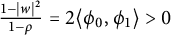 $\frac {1-|w|^2}{1-\rho }=2\langle \phi _0,\phi _1\rangle>0$
by
 $(3)$
. Let
 $u\in C^2({B}^{m},{B}^{n})$
. Then,
 $\tau _0(u)=0$
if and only if
 $$ \begin{align} \begin{aligned} &\rho(1-|u|^2)(1-\rho^2)\Delta_0u+\sum\limits_{i=1}^m2(m-2)(1-|u|^2)\rho x^i\frac{\partial u}{\partial x^i}\\ & \quad +2(1-\rho^2)\rho(2 \langle u , \nabla_0 u \rangle \nabla_0u-\langle \nabla_0 u, \nabla_0 u \rangle u)=0. \end{aligned} \end{align} $$
Lemma 2.2 Let
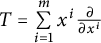 $T=\sum \limits _{i=1}^m x^i\frac {\partial }{\partial x^i}$
. If
 $\phi \in C^2(\overline {{B}^{m}}\backslash \{0\})$
with
 $\phi (x)=\phi (sx), \forall s \in (0,1)$
, then
 $T \phi (x)=0, \forall x\in {B}^{m}.$
Proof
 $\phi (x)=\phi (sx), \forall s \in (0,1)$
. Then, for any
 $x\in \mathbb {B}^{m}$
,
 $$ \begin{align*} T\phi(x)=T(\phi(sx))=\sum\limits_{i=1}^m x^i\frac{\partial}{\partial x^i}\phi(sx)=\sum\limits_{i=1}^m s x^i\frac{\partial \phi}{\partial x^i}(sx)\rightarrow 0, \text{ as } s\rightarrow 0.\\[-43pt] \end{align*} $$
Next, we will calculate equation (2.1) in two parts.
2.1 Computation of
$\rho(1-|u|^2)(1-\rho^2)\Delta_0u+\sum\limits_{i=1}^m2(m-2)(1-|u|^2)\rho x^i\frac{\partial u}{\partial x^i}$

Let
 $d:=\rho -1$
,
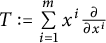 $T:=\sum \limits _{i=1}^{m}x^i\frac {\partial }{\partial x^i}$
. Let
 $\phi _k(x)=\phi _k(sx)$
be smooth functions except the origin and
 $$ \begin{align} \begin{aligned} \phi(x)=\sum\limits_{k=0}^{\infty} \phi_kd(x)^k. \end{aligned} \end{align} $$
For
 $k\geq 0$
with
 $\phi _{-1}=\phi _{-2}=0$
, define
 $$ \begin{align} \begin{aligned} D_k[\phi]=&-[\Delta_0 \phi_{k-3} +3\Delta_0 \phi_{k-2} +2\Delta_0 \phi_{k-1} + (k-1)(k+m-3)\phi_{k-1}\\ &+ k(3k+2m-5)\phi_k+ 2 k(k+1)\phi_{k+1}]+2(m-2)[(k-1)\phi_{k-1}\\ &+2k\phi_k+(k+1)\phi_{k+1}]. \end{aligned} \end{align} $$
Lemma 2.3 Let
 $\phi \in C^\infty (\overline {{B}^{m}},\overline {{B}^{n}})$
with the asymptotic expansion (2.2) near
 $\partial {B}^{m} $
. Then,
 $$ \begin{align} \begin{aligned} \rho(1-\rho^2)\Delta_0\phi+\sum\limits_{i=1}^m2(m-2)\rho x^i\frac{\partial \phi}{\partial x^i}=\sum\limits_{k=0}^{\infty}D_k[\phi]d^k. \end{aligned} \end{align} $$
Proof Notice that for any non-negative integer k and for each i ranging from
 $1$
to m, it holds that
 $$ \begin{align} \begin{aligned} \frac{\partial (\phi_kd^k)}{\partial x^i}&=\frac{\partial \phi_k}{\partial x^i}d^k+k\phi_kd^{k-1}\frac{x^i}{\rho},\\\frac{\partial^2 (\phi_kd^k)}{\partial (x^i)^2} &=\frac{\partial^2 \phi_k}{\partial (x^i)^2}d^k+2k\frac{\partial \phi_k}{\partial x^i}d^{k-1}\frac{x^i}{\rho}\\& \quad +k(k-1)\phi_kd^{k-2}(\frac{x^i}{\rho})^2+k\phi_kd^{k-1}(\frac{1}{\rho}-\frac{(x^i)^2}{\rho^3}). \end{aligned} \end{align} $$
Recall the definitions
 $\rho =d+1, 1-\rho ^2=-d(d+2)$
. Summing the second equation in (2.5) over i from
 $1$
to m and then multiplying the result by
 $\rho (1-\rho ^2)$
, we can calculate
 $\Delta _0(\phi _kd^k)$
multiplied by
 $(1-\rho ^2)\rho $
. According to Lemma 2.2, we have
 $$ \begin{align*} \begin{aligned} &(1-\rho^2)\rho\Delta_0(\phi_kd^k)\\& \quad =-[\Delta_0 \phi_k d^{k+1}(d+1)(d+2)+k(k-1)\phi_kd^{k-1}(d+1)(d+2)\\& \qquad +k(m-1)\phi_kd^{k}(d+2)]\\& \quad =-[\Delta_0 \phi_k d^{k+3} +3\Delta_0 \phi_k d^{k+2} +(2\Delta_0 \phi_k + k(k-1)\phi_k+k(m-1)\phi_k )d^{k+1}\\& \qquad + (3k(k-1)\phi_k+2k(m-1)\phi_k )d^k+ 2 k(k-1)\phi_kd^{k-1}]. \end{aligned} \end{align*} $$
Next, by summing the above expression over k from
 $0$
to
 $\infty $
, we get
 $$ \begin{align} \begin{aligned} &(1-\rho^2)\rho\Delta_0\phi\\& \quad =-[\sum\limits_{k=3}^{\infty}\Delta_0 \phi_{k-3} d^{k} +3\sum\limits_{k=2}^{\infty}\Delta_0 \phi_{k-2} d^{k}\\& \qquad +\sum\limits_{k=1}^{\infty}(2\Delta_0 \phi_{k-1} + (k-1)(k-2)\phi_{k-1}+(k-1)(m-1)\phi_{k-1} )d^{k}\\& \qquad + \sum\limits_{k=0}^{\infty}(3k(k-1)\phi_k+2k(m-1)\phi_k )d^k+ 2 \sum\limits_{k=0}^{\infty}k(k+1)\phi_{k+1}d^{k}]\\& \quad =-\sum\limits_{k=0}^{\infty}[\Delta_0 \phi_{k-3} +3\Delta_0 \phi_{k-2} +2\Delta_0 \phi_{k-1} + (k-1)(k+m-3)\phi_{k-1}\\& \qquad + k(3k+2m-5)\phi_k+ 2 k(k+1)\phi_{k+1}]d^{k}\\& \quad =: \sum\limits_{k=0}^{\infty}D^1_k[\phi]d^k. \end{aligned} \end{align} $$
We multiply the first equation of (2.5) by
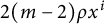 $2(m-2)\rho x^i$
and then sum over i from
 $1$
to m. By applying Lemma 2.2, we can derive
 $$ \begin{align} \begin{aligned} \sum\limits_{i=1}^m2(m-2)\rho x^i\frac{\partial (\phi_kd^k)}{\partial x^i}&= \sum\limits_{i=1}^m2(m-2)\rho x^i(\frac{\partial \phi_k}{\partial x^i}d^k+k\phi_kd^{k-1}\frac{x^i}{\rho})\\&=2(m-2)k\phi_kd^{k-1}(d+1)^2\\&=2(m-2)[k\phi_kd^{k+1}+2k\phi_kd^{k}+k\phi_kd^{k-1}]. \end{aligned} \end{align} $$
We sum equation (2.7) over k from
 $0$
to
 $\infty $
. This summation yields
 $$ \begin{align} \begin{aligned} &\sum\limits_{i=1}^m2(m-2)\rho x^i\frac{\partial \phi}{\partial x^i}\\& \quad =\sum\limits_{k=0}^\infty2(m-2)[k\phi_kd^{k+1}+2k\phi_kd^{k}+k\phi_kd^{k-1}]\\& \quad =\sum\limits_{k=0}^{\infty}2(m-2)[(k-1)\phi_{k-1}d^{k}+2k\phi_kd^{k}+(k+1)\phi_{k+1}d^{k}]\\& \quad =: \sum\limits_{k=0}^{\infty}D^2_k[\phi]d^k. \end{aligned} \end{align} $$
By adding equations (2.6) and (2.8), we obtain
 $$ \begin{align*} \begin{aligned} &(1-\rho^2)\rho\Delta_0\phi+\sum\limits_{i=1}^m2(m-2)\rho x_i\frac{\partial \phi}{\partial x_i}\\& \quad = \sum\limits_{k=0}^{\infty}(D^1_k[\phi]+D^2_k[\phi])d^k = \sum\limits_{k=0}^{\infty}D_k[\phi]d^k. \end{aligned}\\[-41pt] \end{align*} $$
Next, we will use the following notations:
 $$ \begin{align*} \begin{aligned} \psi_l(x)=\sum\limits_{k=1}^{\infty} \psi_{k,l}d^k \text{ with } \psi_{k,l}=0 \text{ when } k<lm+1 \end{aligned} \end{align*} $$
and
 $$ \begin{align*} \begin{aligned} u(x)=\phi(x)+\sum\limits_{l=1}^{\infty} \psi_{l}(x)(\log (-d))^l. \end{aligned} \end{align*} $$
First, we have the operator
 $D_k[u]$
given by
 $$ \begin{align} \begin{aligned} D_k[u]&=D_k[\phi]-2\xi_{k,1}[\psi_{1}]+\eta_{k,1}[\psi_{1}]-(m-1)\zeta_{k,1}[\psi_{1}]-2\eta_{k,2}[\psi_{2}]\\& \quad +2(m-2)(\psi_{k-1,1}+2\psi_{k,1}+\psi_{k+1,1}) \end{aligned} \end{align} $$
and the operator
 $D_{k,l}[u]$
defined as
 $$ \begin{align} \begin{aligned} D_{k,l}[u]&=D_k[\psi_l]-2(l+1 ) \xi_{k,l+1}[\psi_{l+1}]+(l+1 ) \eta_{k,l+1}[\psi_{l+1}]\\& \quad -(l+1)(m-1)\zeta_{k,l+1}[\psi_{l+1}]-(l+1)(l+2)\eta_{k,l+2}[\psi_{l+2}]\\& \quad+ 2(m-2)(l+1)(\psi_{k-1,l+1}+2\psi_{k,l+1}+\psi_{k+1,l+1}), \end{aligned} \end{align} $$
where
 $D_k[\phi ]$
is defined by (2.3) and we have the following definitions for the terms involving
 $\xi _{k,l}[\psi _l]$
,
 $\eta _{k,l}[\psi _l]$
, and
 $\zeta _{k,l}[\psi _l]$
,
 $$ \begin{align} \xi_{k,l}[\psi_l]&=(k-1)\psi_{k-1,l} +3k\psi_{k,l}+2(k+1)\psi_{k+1,l},\end{align} $$
 $$ \begin{align} \begin{aligned} \eta_{k,l}[\psi_l]=\psi_{k-1,l}+3\psi_{k,l}+2\psi_{k+1,l}, \end{aligned} \end{align} $$
 $$ \begin{align} \begin{aligned} \zeta_{k,l}[\psi_l]=\psi_{k-1,l}+2\psi_{k,l}. \end{aligned} \end{align} $$
For the function
 $(\log (-d))^l$
, notice the following partial derivative relationships:
 $$ \begin{align} \begin{aligned} \frac{\partial }{\partial x_i}(\log (-d))^l&=l(\log (-d))^{l-1}\frac{x^i}{d\rho},\\\frac{\partial^2 (\log (-d))^l}{\partial (x^i)^2} &=l(l-1)(\log (-d))^{l-2}\frac{1}{d^2}\frac{(x^i)^2}{\rho^2}\\& \quad -l(\log (-d))^{l-1}\frac{1}{d^2}\frac{(x^i)^2}{\rho^2}+l(\log (-d))^{l-1}\frac{1}{d}(\frac{1}{\rho}-\frac{(x^i)^2}{\rho^3}). \end{aligned} \end{align} $$
Additionally, we have the following summation and Laplacian relationships:
 $$ \begin{align*} \begin{aligned} &\sum\limits_{i=1}^mx^i \frac{\partial (\log (-d))^l}{\partial x^i}=l\frac{d+1}{d}(\log (-d))^{l-1},\\&\Delta_0 (\log (-d))^l\\& \quad =l(l-1)d^{-2}(\log (-d))^{l-2}-ld^{-2}(\log (-d))^{l-1}+l(m-1)d^{-1}\rho^{-1}(\log (-d))^{l-1}. \end{aligned} \end{align*} $$
Let
 $v_l=\psi _l(\log (-d))^l$
. Recall the definitions
 $\rho =d+1, 1-\rho ^2=-d(d+2)$
. According to the second equation in (2.14), we can calculate
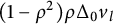 $(1-\rho ^2)\rho \Delta _0 v_l$
,
 $$ \begin{align*} \begin{aligned} &(1-\rho^2)\rho\Delta_0 v_l\\& \quad =(1-\rho^2)\rho[\Delta_0\psi_l (\log (-d))^l+\sum\limits_{i=1}^m2\frac{\partial \psi_l}{\partial x^i}\frac{\partial (\log (-d))^l}{\partial x^i}+\psi_l\Delta_0 (\log (-d))^l]\\& \quad =-[\Delta_0\psi_ld(d+1)(d+2) (\log (-d))^l+\sum\limits_{i=1}^m2(d+2) \frac{\partial \psi_l}{\partial x^i}x^il(\log (-d))^{l-1}\\& \qquad +l(l-1)d^{-1}(d+1)(d+2)\psi_l (\log (-d))^{l-2} -ld^{-1}(d+1)(d+2)\psi_l (\log (-d))^{l-1} \\& \qquad +l(m-1)(d+2)\psi_l (\log (-d))^{l-1}]\\& \quad =-[\Delta_0\psi_ld(d+1)(d+2) (\log (-d))^l\\& \qquad +(2(d+2)l T \psi_l -ld^{-1}(d+1)(d+2)\psi_l +l(m-1)(d+2)\psi_l )(\log (-d))^{l-1}\\& \qquad +l(l-1)d^{-1}(d+1)(d+2)\psi_l (\log (-d))^{l-2}], \end{aligned} \end{align*} $$
where
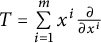 $T=\sum \limits _{i=1}^m x^i\frac {\partial }{\partial x^i}$
. Finally, for the infinite sum
 $\sum \limits _{l=1}^\infty v_l$
, we have
 $$ \begin{align} &(1-\rho^2)\rho\Delta_0 (\sum\limits_{l=1}^\infty v_l)\nonumber\\& \quad =-[\sum\limits_{l=1}^\infty\Delta_0\psi_ld(d+1)(d+2) (\log (-d))^l\nonumber\\& \qquad +\sum\limits_{l=1}^\infty(2(d+2)(l+1 )T \psi_{l+1}-(l+1)d^{-1}(d+1)(d+2)\psi_{l+1}\\& \qquad +(l+1)(m-1)(d+2)\psi_{l+1} )(\log (-d))^{l}\nonumber\\& \qquad +\sum\limits_{l=1}^\infty (l+2)(l+1)d^{-1}(d+1)(d+2)\psi_{l+2} (\log (-d))^{l}+2(d+2)T\psi_1\nonumber\\& \qquad -d^{-1}(d+1)(d+2)\psi_1+(m-1)(d+2)\psi_1+2d^{-1}(d+1)(d+2)\psi_2 ].\nonumber \end{align} $$
Similar to the computation of (2.6), we have
 $$ \begin{align} \begin{aligned} -\sum\limits_{l=1}^\infty\Delta_0\psi_ld(d+1)(d+2) =\rho(1-\rho^2)\Delta_0\psi_l= \sum\limits_{k=1}^{\infty}D^1_k[\psi_l]d^k. \end{aligned} \end{align} $$
By Lemma 2.2,
 $T\psi _{k,l}=0$
. Notice that
 $\psi _{k,l}=0 \text { when } k<ml+1$
. We can compute the term
 $2(d+2)(l+1 )T \psi _{l+1}$
,
 $$ \begin{align*} \begin{aligned} 2(d+2)(l+1 )T \psi_{l+1}&=2(d+2)(l+1 )\sum\limits_{k=1}^{\infty} \psi_{k,l+1} Td^k \\&=2(d+2)(l+1 )\sum\limits_{k=1}^{\infty} \psi_{k,l+1} k(d^k+d^{k-1}). \end{aligned} \end{align*} $$
After arranging according to the powers of d, we can obtain
 $$ \begin{align} \begin{aligned} &2(d+2)(l+1 )T \psi_{l+1}\\& \quad =2(l+1 )\sum\limits_{k=1}^{\infty} k\psi_{k,l+1} (d^{k+1}+3d^k+2d^{k-1}) \\& \quad =2(l+1 )\sum\limits_{k=1}^{\infty} [(k-1)\psi_{k-1,l+1} +3k\psi_{k,l+1}+2(k+1)\psi_{k+1,l+1}]d^k \\& \quad =2(l+1 )\sum\limits_{k=1}^{\infty} \xi_{k,l+1}[\psi_{l+1}]d^k, \end{aligned} \end{align} $$
where
 $\xi _{k,l+1}[\psi _{l+1}]$
is defined in (2.11). Next, we can perform a calculation on the terms
 $(l+1)d^{-1}(d+1)(d+2)\psi _{l+1}$
,
 $(l+1)(m-1)(d+2)\psi _{l+1}$
similar to that on
 $2(d+2)(l+1 )T \psi _{l+1}$
to obtain
 $$ \begin{align} \begin{aligned} &(l+1)d^{-1}(d+1)(d+2)\psi_{l+1}\\& \quad =(l+1)(d^2+3d+2)\sum\limits_{k=1}^{\infty} \psi_{k,l+1} d^{k-1}\\& \quad =(l+1)\sum\limits_{k=1}^{\infty} (\psi_{k-1,l+1}+3\psi_{k,l+1}+2\psi_{k+1,l+1}) d^k\\& \quad =(l+1 )\sum\limits_{k=1}^{\infty} \eta_{k,l+1}[\psi_{l+1}]d^k, \end{aligned} \end{align} $$
where
 $\eta _{k,l+1}[\psi _{l+1}]$
is defined in (2.12) and
 $$ \begin{align} \begin{aligned} (l+1)(m-1)(d+2)\psi_{l+1}&= (l+1)(m-1)(d+2)\sum\limits_{k=1}^{\infty} \psi_{k,l+1} d^{k}\\& =(l+1)(m-1)\sum\limits_{k=1}^{\infty} (\psi_{k-1,l+1}+2\psi_{k,l+1}) d^{k}\\& =(l+1)(m-1)\sum\limits_{k=1}^{\infty} \zeta_{k,l+1}[\psi_{l+1}]d^k, \end{aligned} \end{align} $$
where
 $\zeta _{k,l+1}[\psi _{l+1}]$
is defined in (2.13). And finally,
 $$ \begin{align} \begin{aligned} & (l+2)(l+1)d^{-1}(d+1)(d+2)\psi_{l+2}\\& \quad = (l+1)(l+2)\sum\limits_{k=1}^{\infty} (\psi_{k-1,l+2}+3\psi_{k,l+2}+2\psi_{k+1,l+2}) d^k\\& \quad =(l+1)(l+2)\sum\limits_{k=1}^{\infty} \eta_{k,l+2}[\psi_{l+2}]d^k. \end{aligned} \end{align} $$
Therefore substituting (2.16)–(2.20) into (2.15), we have
 $$ \begin{align} \begin{aligned} &(1-\rho^2)\rho\Delta_0 (\sum\limits_{l=1}^\infty v_l)\\& \quad =\sum\limits_{l=1}^\infty\sum\limits_{k=1}^{\infty}(D^1_k[\psi_l]-2(l+1 ) \xi_{k,l+1}[\psi_{l+1}]+(l+1 ) \eta_{k,l+1}[\psi_{l+1}]\\& \qquad -(l+1)(m-1)\zeta_{k,l+1}[\psi_{l+1}]-(l+1)(l+2)\eta_{k,l+2}[\psi_{l+2}])d^k(\log (-d))^l\\& \qquad +\sum\limits_{k=1}^{\infty}( -2\xi_{k,1}[\psi_{1}]+\eta_{k,1}[\psi_{1}]-(m-1)\zeta_{k,1}[\psi_{1}]-2\eta_{k,2}[\psi_{2}])d^k. \end{aligned} \end{align} $$
For the second part,
 $$ \begin{align*} \begin{aligned} &2(m-2)\rho\sum\limits_{i=1}^m x_i\frac{\partial v_l}{\partial x_i}=2(m-2)\rho[\sum\limits_{i=1}^m x_i\frac{\partial \psi_l}{\partial x_i}(\log (-d))^l+\psi_lx^i\frac{\partial (\log (-d))^l}{\partial x^i}]\\& \quad =\sum\limits_{k=1}^{\infty} D_k^2[\psi_l] d^k (\log (-d))^l+2(m-2)l\psi_l(d+2+\frac{1}{d})(\log (-d))^{l-1}. \end{aligned} \end{align*} $$
Summing l from
 $1$
to
 $\infty $
, we get
 $$ \begin{align} \\[-18pt] &2(m-2)\rho\sum\limits_{i=1}^m x_i\frac{\partial }{\partial x_i}(\sum\limits_{l=1}^\infty v_l)\nonumber\\& \quad =\sum\limits_{l=1}^\infty \sum\limits_{k=1}^{\infty} D_k^2[\psi_l] d^k (\log (-d))^l+\sum\limits_{l=1}^\infty 2(m-2)l\psi_l(d+2+\frac{1}{d})(\log (-d))^{l-1}\nonumber\\& \quad =\sum\limits_{l=1}^\infty \sum\limits_{k=1}^{\infty} D_k^2[\psi_l] d^k (\log (-d))^l\nonumber\\& \qquad +\sum\limits_{l=1}^\infty 2(m-2)(l+1)\psi_{l+1}(d+2+\frac{1}{d})(\log (-d))^{l}+2(m-2)\psi_1(d+2+\frac{1}{d})\nonumber\\& \quad =\sum\limits_{l=1}^\infty \sum\limits_{k=1}^{\infty} (D_k^2[\psi_l]+ 2(m-2)(l+1)(\psi_{k-1,l+1}+2\psi_{k,l+1}+\psi_{k+1,l+1}))\nonumber\\& \qquad \times d^k (\log (-d))^l+2(m-2)\sum\limits_{k=1}^{\infty}(\psi_{k-1,1}+2\psi_{k,1}+\psi_{k+1,1})d^k .\nonumber \end{align} $$
Therefore the summation of equations (2.21), (2.22), and (2.4) yields
 $$ \begin{align*} \begin{aligned} &((1-\rho^2)\rho\Delta_0 +2(m-2)\rho T)(\phi+\sum\limits_{l=1}^{\infty} \psi_{l}(x)(\log (-d))^l)\\& \quad =\sum\limits_{k=0}^{\infty}D_k[u]d^k+\sum\limits_{l=1}^\infty \sum\limits_{k=1}^{\infty}D_{k,l}[u] d^k (\log (-d))^l, \end{aligned} \end{align*} $$
where
 $D_k[u]$
and
 $D_{k,l}[u]$
are defined in (2.9) and (2.10).
As a summary, we have proved the following lemma.
Lemma 2.4 Let
 $\psi _{k,l}=0$
when
 $k<ml+1$
and let
 $$ \begin{align} \begin{aligned} u(x)=\sum\limits_{k=0}^{\infty}\phi_k(x)d^k+\sum\limits_{l=1}^{\infty}\sum\limits_{k=1}^{\infty} \psi_{k,l}(x)d^k(\log (-d))^l. \end{aligned} \end{align} $$
Then
 $$ \begin{align*} \begin{aligned} &((1-\rho^2)\rho\Delta_0 +2(m-2)\rho T)u(x)\\& \quad =\sum\limits_{k=0}^{\infty}D_k[u]d^k+\sum\limits_{l=1}^\infty \sum\limits_{k=1}^{\infty}D_{k,l}[u] d^k (\log (-d))^l, \end{aligned} \end{align*} $$
where
 $D_k[u]$
and
 $D_{k,l}[u]$
are defined in (2.9) and (2.10).
Define
 $$ \begin{align*} \begin{aligned} A_{p,q}[\phi]:=\langle \phi_p,\phi_q\rangle, \ A_k[\phi]:=\sum\limits_{p+q=k} A_{p,q}[\phi], \end{aligned} \end{align*} $$
 $$ \begin{align*} \begin{aligned} {A}_{k,l}[u]:=\sum\limits_{\alpha+\beta=k}(\langle \phi_\alpha,\psi_{\beta,l}\rangle+\langle\phi_\beta,\psi_{\alpha,l}\rangle)+\sum\limits_{s+t=l}\sum\limits_{\alpha+\beta=k}\langle\psi_{\alpha,s},\psi_{\beta,t}\rangle, \end{aligned} \end{align*} $$
 $$ \begin{align} \begin{aligned} B_k[u]:=-\sum\limits_{\alpha+\beta=k}A_\alpha[\phi]D_\beta[u], \end{aligned} \end{align} $$
and
 $$ \begin{align} \begin{aligned} B_{k,l}[u]&:=-\sum\limits_{\alpha+\beta=k}(A_\alpha[\phi]D_{\beta,l}[u]+{A}_{\alpha,l}D_\beta[u])\\& \quad -\sum\limits_{s+t=l}\sum\limits_{\alpha+\beta=k}{A}_{\alpha,s}[u]D_{\beta,t}[u]. \end{aligned} \end{align} $$
Theorem 2.5 Let u be defined in (2.23) with
 $|\phi _0|=1$
, then
 $$ \begin{align*} \begin{aligned} &(1-|u|^2)((1-\rho^2)\rho\Delta_0 +2(m-2)\rho T)u(x)\\& \quad =\sum\limits_{k=0}^{\infty}B_k[u]d^k+\sum\limits_{l=1}^\infty \sum\limits_{k=1}^{\infty}B_{k,l}[u] d^k (\log (-d))^l. \end{aligned} \end{align*} $$
Proof According to the expression of u, we have
 $$ \begin{align*} \begin{aligned} 1-|u|^2&=1-\sum\limits_{k=0}^{\infty}\sum\limits_{\alpha+\beta=k}\langle\phi_\alpha,\phi_\beta\rangle d^k\\& \quad -\sum\limits_{l=1}^\infty \sum\limits_{k=1}^{\infty}\sum\limits_{\alpha+\beta=k}(\langle \phi_\alpha,\psi_{\beta,l}\rangle+\langle\phi_\beta,\psi_{\alpha,l}\rangle)d^k(\log(-d))^l\\& \quad -\sum\limits_{l=1}^\infty \sum\limits_{k=1}^{\infty}\sum\limits_{\alpha+\beta=k}\sum\limits_{s+t=l}\langle \psi_{\alpha,s},\psi_{\beta,t}\rangle d^k(\log(-d))^l. \end{aligned} \end{align*} $$
Since
 $\langle \phi _0,\phi _0\rangle =1$
, we can get
 $$ \begin{align*} \begin{aligned} 1-|u|^2=&-\sum\limits_{k=1}^{\infty}A_k[\phi]d^k-\sum\limits_{l=1}^\infty \sum\limits_{k=1}^{\infty}A_{l,k}[u]d^k(\log(-d))^l. \end{aligned} \end{align*} $$
By Lemma 2.4, substituting the expression for
 $1-|u|^2$
obtained above, we get
 $$ \begin{align*} \begin{aligned} &\quad -(1-|u|^2)((1-\rho^2)\rho\Delta_0 +2(m-2)\rho T)u(x)\\&=\sum\limits_{k=1}^{\infty} \sum\limits_{\alpha+\beta=k}A_\alpha[\phi]D_\beta[u] d^k\\& \quad +\sum\limits_{l=1}^\infty \sum\limits_{k=1}^{\infty}\sum\limits_{\alpha+\beta=k}(A_\alpha[\phi]D_{\beta,l}[u]+A_{\alpha,l}D_\beta[u])d^k(\log(-d))^l\\& \quad +\sum\limits_{l=1}^\infty \sum\limits_{k=1}^{\infty}\sum\limits_{\alpha+\beta=k}\sum\limits_{s+t=l}A_{\alpha,s}[u]D_{\beta,t}[u]d^k(\log(-d))^l\\&=-\sum\limits_{k=1}^{\infty}B_k[u]d^k-\sum\limits_{l=1}^\infty \sum\limits_{k=1}^{\infty}B_{k,l}[u]d^k(\log(-d))^l. \end{aligned} \end{align*} $$
The proof of the proposition is complete.
2.2 Computation of
$2(1-\rho ^2)\rho (2 \langle u , \nabla _0 u \rangle \nabla _0u-\langle \nabla _0 u, \nabla _0 u \rangle u)$

Given that
 $ u(x)=\sum \limits _{k=0}^{\infty }\phi _k(x)d^k+\sum \limits _{l=1}^{\infty }\sum \limits _{k=1}^{\infty } \psi _{k,l}(x)d^k(\log (-d))^l$
, we can proceed to calculate its partial derivative with respect to
 $x_i$
,
 $$ \begin{align} \begin{aligned} \frac{\partial u}{\partial x_i}&= \sum\limits_{k=0}^{\infty}(\frac{\partial \phi_k}{\partial x_i}d^k+k\phi_kd^{k-1}\frac{x_i}{\rho})+\sum\limits_{l=1}^\infty \sum\limits_{k=1}^{\infty}[\frac{\partial \psi_{k,l}}{\partial x_i} d^k(\log (-d))^l\\& \quad +k \psi_{k,l}d^{k-1}\frac{x_i}{\rho}(\log (-d))^l+l \psi_{k,l}d^{k-1}\frac{x_i}{\rho}(\log (-d))^{l-1}]\\&= \sum\limits_{k=0}^{\infty}(\frac{\partial \phi_k}{\partial x_i}d^k+[(k+1)\phi_{k+1}+\psi_{k+1,1}] d^{k}\frac{x_i}{\rho}\\& \quad +\sum\limits_{l=1}^\infty \sum\limits_{k=1}^{\infty}\frac{\partial \psi_{k,l}}{\partial x_i} d^k(\log (-d))^l\\& \quad +[(k+1) \psi_{k+1,l}+(l+1) \psi_{k+1,l+1}]d^{k}\frac{x_i}{\rho}(\log (-d))^l. \end{aligned} \end{align} $$
Recall that the definition of
 $\langle \cdot ,\cdot \rangle $
, we can compute
 $$ \begin{align} \begin{aligned} &\langle u, \frac{\partial u}{\partial x_i} \rangle \frac{\partial u}{\partial x_i}=\sum\limits_{k=0}^{\infty}\Omega_kd^k+\sum\limits_{l=1}^{\infty}\sum\limits_{k=m}^{\infty} \sum\limits_{p+q+j=k} \Omega_{pqj}d^{k} (\log (-d))^l\\& \quad +\sum\limits_{l=1}^{\infty}\sum\limits_{k=1}^{\infty} \sum\limits_{p+q+j=k}\sum\limits_{\alpha+\beta=l}\Omega_{pqj\alpha\beta}d^{k} (\log (-d))^l\\& \quad +\sum\limits_{l=1}^{\infty}\sum\limits_{k=1}^{\infty} \sum\limits_{p+q+j=k}\sum\limits_{\alpha+\beta+\gamma=l} \Omega_{pqj\alpha\beta\gamma}d^{k} (\log (-d))^l. \end{aligned} \end{align} $$
Here, the coefficients
 $\Omega _k$
,
 $\Omega _{pqj}$
,
 $\Omega _{pqj\alpha \beta }$
, and
 $\Omega _{pqj\alpha \beta \gamma }$
are defined as follows:
 $$ \begin{align*} \begin{aligned} \Omega_k&=\sum\limits_{p+q+j=k} \langle \frac{\partial \phi_p}{\partial x_i}, \phi_{q} \rangle\frac{\partial \phi_j}{\partial x_i}\\& \quad +\left(\langle \frac{\partial \phi_p}{\partial x_i}, \phi_{q} \rangle(((j+1)\phi_{j+1}+\psi_{j+1,1}))+\langle(p+1)\phi_{p+1}+\psi_{p+1,1},\phi_q\rangle\frac{\partial \phi_j}{\partial x_i} \right)\frac{x_i}{\rho}\\& \quad +\left( \langle (p+1)\phi_{p+1}+\psi_{p+1,1},\phi_q \rangle [(j+1)\phi_{j+1}+\psi_{j+1,1} ] \right)(\frac{x_i}{\rho})^2, \end{aligned} \end{align*} $$
and
 $$ \begin{align*} \begin{aligned} &\Omega_{pqj}=( \langle \frac{\partial \psi_{p,l}}{\partial x_i} ,\phi_q \rangle \frac{\partial \phi_j}{\partial x_i} + \langle \frac{\partial \phi_p}{\partial x_i},\phi_q \rangle \frac{\partial \psi_{j,l}}{\partial x_i}+\langle \frac{\partial \phi_p}{\partial x_i},\psi_{q,l}\rangle \frac{\partial \phi_{j}}{\partial x_i} )\\& \quad +\left( \langle \frac{\partial \psi_{p,l}}{\partial x_i} ,\phi_q \rangle [(j+1)\phi_{j+1}+\psi_{j+1,1}]+\langle (p+1)\psi_{p+1,l}+(l+1)\psi_{p+1,l+1}, \phi_q \rangle \frac{\partial \phi_j}{\partial x_i}\right.\\& \quad \left.+ \langle (p+1)\phi_{p+1}+\psi_{p+1,1},\phi_q \rangle \frac{\partial \psi_{j,l}}{\partial x_i}+\langle \frac{\partial \phi_p}{\partial x_i} , \phi_q\rangle [(j+1)\psi_{j+1,l}+(l+1)\psi_{j+1,l+1}]\right.\\& \quad \left.+ \langle \frac{\partial \phi_{p}}{\partial x_i},\psi_{q,l} \rangle [(j+1)\phi_{j+1}+\psi_{j+1,1}] +\langle (p+1)\phi_{p+1}+\psi_{p+1,1},\psi_{q,l} \rangle \frac{\partial \phi_{j}}{\partial x_i} \right)\frac{x^i}{\rho}\\& \quad +\left(\langle (p+1)\phi_{p+1}+\psi_{p+1,1} ,\phi_q \rangle[(j+1)\psi_{j+1,l}+(l+1)\psi_{j+1,l+1}] \right.\\& \quad \left.+\langle (p+1)\phi_{p+1}+\psi_{p+1,1},\psi_{q,l} \rangle [(j+1)\phi_{j+1}+\psi_{j+1,1}] \right.\\& \quad \left.+\langle (p+1)\psi_{p+1,l}+(l+1)\psi_{p+1,l+1} ,\phi_q \rangle [(j+1)\phi_{j+1}+\psi_{j+1,1}] \right) (\frac{x_i}{\rho})^2 , \end{aligned} \end{align*} $$
and the expressions of
 $\Omega _{pqj\alpha \beta }$
and
 $\Omega _{pqj\alpha \beta \gamma }$
are omitted for the sake of brevity.
Sum for i from
 $1$
to m and multiply
 $\rho $
in (2.27) to find
 $$ \begin{align*} &\rho \langle u, \nabla u \rangle \nabla u =\sum\limits_{k=0}^{\infty} \sum\limits_{p+q+j=k} (\langle \phi_{p} , \nabla \phi_q \rangle \nabla\phi_j\\& \quad +\langle(p+1)\phi_{p+1}+\psi_{p+1,1},\phi_q\rangle [(j+1)\phi_{j+1}+\psi_{j+1,1}])d^k(d+1)\\& \quad +\sum\limits_{l=1}^{\infty}\sum\limits_{k=m}^{\infty} \sum\limits_{p+q+j=k} ( \langle \nabla\psi_{p,l}, \phi_q \rangle \nabla \phi_j + \langle\nabla \phi_p, \phi_q \rangle \nabla \phi_{j,l}+\langle \nabla\phi_p, \psi_{q,l}\rangle \nabla\phi_j \\& \quad +\langle(p+1)\phi_{p+1}+\psi_{p+1,1},\phi_q\rangle[(j+1)\psi_{j+1,l}+(l+1)\psi_{j+1,l+1}]\\& \quad +\langle(p+1)\phi_{p+1}+\psi_{p+1,1},\psi_{q,l}\rangle[(j+1)\phi_{j+1}+\psi_{j+1,1}]\\& \quad +\langle(p+1)\psi_{p+1,l}+(l+1)\psi_{p+1,l+1},\phi_q\rangle[(j+1)\phi_{j+1}+\psi_{j+1,1}]) d^{k} (d+1)(\log (-d))^l\\& \quad +\sum\limits_{l=1}^{\infty}\sum\limits_{k=1}^{\infty} \sum\limits_{p+q+j=k}(\sum\limits_{\alpha+\beta=l}\Lambda_{pqj\alpha\beta}+\sum\limits_{\alpha+\beta+\gamma=l} \Lambda_{pqj\alpha\beta\gamma}) d^{k}(d+1) (\log (-d))^l, \end{align*} $$
where
 $\Lambda _{pqj\alpha \beta }$
and
 $\Lambda _{pqj\alpha \beta \gamma }$
are omitted for the sake of brevity.
Define
 $H_k[u]$
and
 $H_{k,l}[u]$
such that
 $$ \begin{align*} \begin{aligned} &\rho \langle u, \nabla u \rangle \nabla u =:\sum\limits_{k=0}^{\infty} H_k[u]d^k+\sum\limits_{l=1}^{\infty}\sum\limits_{k=1}^{\infty} H_{k,l}[u]d^k(\log (-d))^l. \end{aligned} \end{align*} $$
Consider
 $1-\rho ^2=-d(d+2)$
. By multiplying both sides of the equation
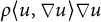 $\rho \langle u, \nabla u \rangle \nabla u$
by
 $4(1-\rho ^2)$
, we get
 $$ \begin{align*} \begin{aligned} &4(1-\rho^2)\rho \langle u, \nabla u \rangle \nabla u=-4d(d+2)\rho \langle u, \nabla u \rangle \nabla u\\& \quad =-4(\sum\limits_{k=2}^{\infty} H_{k-2}[u]d^k+\sum\limits_{l=1}^{\infty}\sum\limits_{k=3}^{\infty} H_{k-2,l}[u]d^k(\log (-d))^l)\\& \qquad -8(\sum\limits_{k=1}^{\infty} H_{k-1}[u]d^k+\sum\limits_{l=1}^{\infty}\sum\limits_{k=2}^{\infty} H_{k-1,l}[u]d^k(\log (-d))^l)\\& \quad =:\sum\limits_{k=1}^{\infty} F_{k}[u]d^k+\sum\limits_{l=1}^{\infty}\sum\limits_{k=2}^{\infty} F_{k,l}[u]d^k(\log (-d))^l, \end{aligned} \end{align*} $$
where
 $$ \begin{align} \begin{aligned} F_{k}[u]=-4 H_{k-2}[u]-8 H_{k-1}[u] \end{aligned} \end{align} $$
and
 $$ \begin{align} \begin{aligned} F_{k,l}[u]=-4 H_{k-2,l}[u]-8 H_{k-1,l}[u]. \end{aligned} \end{align} $$
According to the expression of (2.23) and (2.26), we deduce
 $$ \begin{align} \begin{aligned} \langle \frac{\partial u}{\partial x^i}, \frac{\partial u}{\partial x^i} \rangle u &=\sum\limits_{k=0}^{\infty}X_kd^k+\sum\limits_{l=1}^{\infty}\sum\limits_{k=m}^{\infty} \sum\limits_{p+q+j=k} X_{pqj}d^{k} (\log (-d))^l\\& \quad +\sum\limits_{l=1}^{\infty}\sum\limits_{k=1}^{\infty} \sum\limits_{p+q+j=k}\sum\limits_{\alpha+\beta=l}X_{pqj\alpha\beta}d^{k} (\log (-d))^l\\& \quad +\sum\limits_{l=1}^{\infty}\sum\limits_{k=1}^{\infty} \sum\limits_{p+q+j=k}\sum\limits_{\alpha+\beta+\gamma=l} X_{pqj\alpha\beta\gamma}d^{k} (\log (-d))^l, \end{aligned} \end{align} $$
where
 $$ \begin{align*} \begin{aligned} X_{k} &= \sum\limits_{p+q+j=k}\langle \frac{\partial \phi_p}{\partial x^i} , \frac{\partial \phi_q}{\partial x^i} \rangle \phi_j +\langle \frac{\partial \phi_p}{\partial x^i},(q+1)\phi_{q+1}+\psi_{q+1,1} \rangle \phi_j\frac{x^i}{\rho}\\& \quad +\langle(p+1)\phi_{p+1}+\psi_{p+1,1} ,(q+1)\phi_{q+1}+\psi_{q+1,1} \rangle \phi_j(\frac{x^i}{\rho})^2, \end{aligned} \end{align*} $$
and
 $$ \begin{align*} \begin{aligned} &X_{pqj} =\left(\langle \frac{\partial \phi_p}{\partial x^i} , \frac{\partial \phi_q}{\partial x^i} \rangle \psi_{j,l}+ \langle \frac{\partial \phi_p}{\partial x^i} , \frac{\partial \psi_{q,l}}{\partial x^i} \rangle \phi_j \right )+\left(\langle \frac{\partial \phi_p}{\partial x^i} , (q+1)\phi_{q+1}+\psi_{q+1,1} \rangle \psi_{j,l}\right.\\& \quad \left.+ \langle \frac{\partial \phi_p}{\partial x^i} , (q+1)\psi_{q+1,l}+(l+1)\psi_{q+1,l+1} \rangle \phi_j+ \langle (p+1)\phi_{p+1}+\psi_{p+1,1}, \frac{\partial \psi_{q,l}}{\partial x^i} \rangle \phi_{j} \right) \frac{x^i}{\rho}\\& \quad +(\langle (p+1)\phi_{p+1}+\psi_{p+1,1} ,(q+1)\phi_{q+1}+\psi_{q+1,1} \rangle \psi_{j,l}\\& \quad + \langle (p+1)\phi_{p+1}+\psi_{p+1,1} , (q+1)\psi_{q+1,l}+(l+1)\psi_{q+1,l+1} \rangle \phi_j ) (\frac{x^i}{\rho})^2, \end{aligned} \end{align*} $$
and
 $X_{pqj\alpha \beta }$
and
 $X_{pqj\alpha \beta \gamma }$
are omitted for the sake of brevity.
Summing i from
 $1$
to m and multiplying
 $\rho $
in (2.30), we find that
 $$ \begin{align*} \begin{aligned} &\rho\langle \nabla u, \nabla u \rangle u\\& \quad =\sum\limits_{k=0}^{\infty} \sum\limits_{p+q+j=k} (\langle \nabla \phi_p, \nabla \phi_q \rangle \phi_j +\langle(p+1)\phi_{p+1}+\psi_{p+1,1} ,(q+1)\phi_{q+1}+\psi_{q+1,1} \rangle \phi_j)\\& \qquad \times d^k(d+1) +\sum\limits_{l=1}^{\infty} \sum\limits_{k=1}^{\infty} \sum\limits_{p+q+j=k}(\langle \nabla \phi_p , \nabla\phi_q \rangle \psi_{j,l}+ \langle \nabla \phi_p , \nabla \psi_{q,l}\rangle \phi_j \\& \qquad +\langle (p+1)\phi_{p+1}+\psi_{p+1,1} ,(q+1)\phi_{q+1}+\psi_{q+1,1} \rangle \psi_{j,l}\\& \qquad + \langle (p+1)\phi_{p+1}+\psi_{p+1,1} , (q+1)\psi_{q+1,l}+(l+1)\psi_{q+1,l+1} \rangle \phi_j ) d^k(d+1)(\log (-d))^l\\& \qquad +\sum\limits_{l=2}^{\infty}\sum\limits_{k=1}^{\infty} \sum\limits_{p+q+j=k}(\sum\limits_{\alpha+\beta=l}\Xi_{pqj\alpha\beta}+\sum\limits_{\alpha+\beta+\gamma=l} \Xi_{pqj\alpha\beta\gamma}) d^{k}(d+1) (\log (-d))^l, \end{aligned} \end{align*} $$
where
 $\Xi _{pqj\alpha \beta }$
and
 $\Xi _{pqj\alpha \beta \gamma }$
are omitted for the sake of brevity.
Define
 $W_k[u]$
and
 $W_{k,l}[u]$
such that
 $$ \begin{align*} \begin{aligned} \rho \langle \nabla u, \nabla u \rangle u =:\sum\limits_{k=0}^{\infty} W_k[u]d^k+\sum\limits_{l=1}^{\infty}\sum\limits_{k=1}^{\infty} W_{k,l}[u]d^k(\log (-d))^l. \end{aligned} \end{align*} $$
Then, by multiplying both sides of the equation
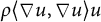 $\rho \langle \nabla u, \nabla u \rangle u$
by
 $-2(1-\rho ^2)$
, we conclude that
 $$ \begin{align*} \begin{aligned} & \quad -2(1-\rho^2)\rho\langle \nabla u, \nabla u \rangle u=2d(d+2)\rho\langle \nabla u, \nabla u \rangle u\\& =2(\sum\limits_{k=2}^{\infty} W_{k-2}[u]d^k+\sum\limits_{l=1}^{\infty}\sum\limits_{k=3}^{\infty} W_{k-2,l}[u]d^k(\log (-d))^l)\\& \quad +4(\sum\limits_{k=1}^{\infty} W_{k-1}[u]d^k+\sum\limits_{l=1}^{\infty}\sum\limits_{k=2}^{\infty} W_{k-1,l}[u]d^k(\log (-d))^l)\\& =:\sum\limits_{k=1}^{\infty} E_{k}[u]d^k+\sum\limits_{l=1}^{\infty}\sum\limits_{k=2}^{\infty} E_{k,l}[u]d^k(\log (-d))^l, \end{aligned} \end{align*} $$
where
 $$ \begin{align} \begin{aligned} E_{k}[u]=2 W_{k-2}[u]+4 W_{k-1}[u] \end{aligned} \end{align} $$
and
 $$ \begin{align} \begin{aligned} E_{k,l}[u]=2 W_{k-2,l}[u]+4 W_{k-1,l}[u]. \end{aligned} \end{align} $$
Lemma 2.6 With the notations above, one has
 $$ \begin{align*} \begin{aligned} &2(1-\rho^2)\rho(2 \langle u , \nabla_0 u \rangle \nabla_0u-\langle \nabla_0 u, \nabla_0 u \rangle u)\\& \quad =\sum\limits_{k=1}^{\infty} (F_{k}[u]+E_{k}[u])d^k+\sum\limits_{l=1}^{\infty}\sum\limits_{k=2}^{\infty} (F_{k,l}[u]+E_{k,l}[u])d^k(\log (-d))^l. \end{aligned} \end{align*} $$
2.3 Proof of Theorem 2.1
Theorem 2.7 With the notations above, one has
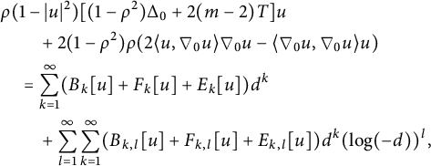 $$ \begin{align*} \begin{aligned} &\rho(1-|u|^2)[(1-\rho^2)\Delta_0+2(m-2) T]u\\& \qquad +2(1-\rho^2)\rho(2 \langle u , \nabla_0 u \rangle \nabla_0u-\langle \nabla_0 u, \nabla_0 u \rangle u)\\& \quad =\sum\limits_{k=1}^{\infty} (B_{k}[u]+F_{k}[u]+E_{k}[u])d^k\\& \qquad +\sum\limits_{l=1}^{\infty}\sum\limits_{k=1}^{\infty} (B_{k,l}[u]+F_{k,l}[u]+E_{k,l}[u])d^k(\log (-d))^l, \end{aligned} \end{align*} $$
where
 $B_k$
and
 $B_{k,l}$
are given by (2.24) and (2.25),
 $F_k$
and
 $F_{k,l}$
are given by (2.28) and (2.29), and
 $E_k$
and
 $E_{k,l}$
are given by (2.31) and (2.32).
From the definition of
 $B_{k,l} , F_{k,l}$
, and
 $E_{k,l}$
, one has
 $$ \begin{align*} \begin{aligned} B_{k,l} =F_{k,l}=E_{k,l}=0 \text{ for } k<ml+1. \end{aligned} \end{align*} $$
Theorem 2.7 implies that if
 $\tau _0(u)=0$
, then
 $$ \begin{align*} \left\{ \begin{aligned} &B_{k}[u]+E_{k}[u]+F_{k}[u]=0, k\geq1,\\&B_{k,l}[u]+E_{k,l}[u]+F_{k,l}[u]=0, l\geq1, k\geq ml+1. \end{aligned} \right. \end{align*} $$
We will solve
 $\phi _k$
and
 $\psi _{k,l}$
through the above system of equations.
Let’s analyze the coefficients
 $B_k$
for different values of k. When
 $k=1$
, the coefficient
 $B_1[u]$
is given by
 $$ \begin{align} \begin{aligned} B_1[u]=-A_1[\phi]D_0[u], \end{aligned} \end{align} $$
where
 $A_1[\phi ]=2\langle \phi _0,\phi _1\rangle , D_0[u]=D_0[\phi ]=2(m-2)\phi _1$
. When
 $2\leq k \leq m$
, the coefficient
 $B_k[u]$
can be expressed as
 $$ \begin{align} \begin{aligned} B_k[u]=-\sum\limits_{q=1}^{k}A_q[\phi]D_{k-q}[u]=-A_kD_0-\sum\limits_{q=1}^{k-1}A_q[\phi]D_{k-q}[u]. \end{aligned} \end{align} $$
Since
 $1\leq k-q\leq m-1$
, we have
 $D_{k-q}[u]=D_{k-q}[\phi ]$
. Recall that
 $A_{p,q}[\phi ]=\langle \phi _p, \phi _q \rangle $
and
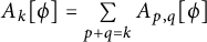 $A_k[\phi ]= \sum \limits _{p+q=k}A_{p,q}[\phi ]$
. When
 $1\leq k\leq m-1$
, according to (2.3), we have
 $$ \begin{align} \begin{aligned} D_k[\phi]&=-[\Delta_0 \phi_{k-3} +3\Delta_0 \phi_{k-2} +2\Delta_0 \phi_{k-1}] + (k-1)(m-k-1)\phi_{k-1}\\& \quad + k(2m-3k-3)\phi_k+ 2 (k+1)(m-2-k)\phi_{k+1}\\& =:2 (k+1)(m-2-k)\phi_{k+1}+\widetilde{D}[\phi_k,\phi_{k-1},\phi_{k-2},\phi_{k-3}], \end{aligned} \end{align} $$
where
 $\widetilde {D}[\phi _k,\phi _{k-1},\phi _{k-2},\phi _{k-3}]$
is determined by
 $\phi _k,\phi _{k-1},\phi _{k-2},\phi _{k-3}$
.
Let us examine the coefficients
 $F_k$
for different values of k. When
 $k=1$
, the coefficient
 $F_1[u]$
is given by
 $$ \begin{align} \begin{aligned} F_1[u]=-8H_0[u], H_0[u]=\langle \phi_0,\nabla \phi_0\rangle\nabla\phi_0+\langle \phi_0, \phi_1\rangle\phi_1=\langle \phi_0, \phi_1\rangle\phi_1\end{aligned} \end{align} $$
and for
 $2\leq k \leq m$
, the coefficient
 $F_k[u]$
is defined by
 $$ \begin{align} \begin{aligned} F_k[u]&=-4H_{k-2}[u]-8H_{k-1}[u]\\&=-8k\langle \phi_0, \phi_k\rangle\phi_1-8k\langle \phi_0, \phi_1\rangle\phi_k+\widetilde{F}[\phi_0,\ldots, \phi_{k-1}] , \end{aligned} \end{align} $$
where
 $\widetilde {F}[\phi _0,\ldots , \phi _{k-1}] $
depends on
 $\phi _0,\ldots , \phi _{k-1}$
.
Let us focus on the coefficients
 $E_k$
and analyze their expressions for different values of k. When
 $k=1$
, the coefficient
 $E_1[u]$
is given by
 $$ \begin{align} \begin{aligned} E_1[u]=4W_0[u], W_0[u]=\langle\nabla\phi_0,\nabla\phi_0\rangle\phi_0+\langle\phi_1,\phi_1\rangle\phi_0 \end{aligned} \end{align} $$
and for
 $2\leq k \leq m$
, the coefficient
 $E_k[u]$
is defined through a combination of
 $W_{k-2}[u]$
and
 $W_{k-1}[u]$
,
 $$ \begin{align} \begin{aligned} E_k[u]=2W_{k-2}[u]+4W_{k-1}[u]=8k\langle\phi_k,\phi_1\rangle\phi_0+\widetilde{E}[\phi_0,\ldots, \phi_{k-1}], \end{aligned} \end{align} $$
where
 $\widetilde {E}[\phi _0,\ldots , \phi _{k-1}] $
depends on
 $\phi _0,\ldots , \phi _{k-1}$
.
2.3.1
$B_{1}[u]+E_{1}[u]+F_{1}[u]=0$

According to (2.33), (2.36), and (2.38),
 $ B_1+E_1+F_1=0$
yields
 $$ \begin{align} \begin{aligned} -m\langle\phi_0,\phi_1\rangle\phi_1+ \langle\nabla\phi_0,\nabla\phi_0\rangle\phi_0+\langle\phi_1,\phi_1\rangle\phi_0=0, \end{aligned} \end{align} $$
where we have used
 $|\phi _0|^2=1$
and
 $\langle \phi _0, \partial _{x^i}\phi _0\rangle =0$
. Then, multiplying (2.40) by
 $\phi _0$
and
 $\phi _1$
, respectively, we get
 $$ \begin{align*} \left\{ \begin{aligned} -mA_{1,0}^2+A_{1,1}+\langle\nabla\phi_0,\nabla\phi_0 \rangle&=0,\\(1-m)A_{1,0}A_{1,1}+\langle\nabla\phi_0,\nabla\phi_0 \rangle A_{1,0}&=0. \end{aligned} \right. \end{align*} $$
Choosing
 $A_1>0$
, we can get
 $$ \begin{align} \begin{aligned} A_{1,1}=A_{1,0}^2=\frac{\langle\nabla\phi_0,\nabla\phi_0 \rangle}{m-1}. \end{aligned} \end{align} $$
So we can solve
 $\phi _1$
from (2.40) that
 $$ \begin{align} \begin{aligned} \phi_1=\frac{ \langle\nabla\phi_0,\nabla\phi_0\rangle\phi_0+\langle\phi_1,\phi_1\rangle\phi_0}{m\langle\phi_0,\phi_1\rangle}=\sqrt{\dfrac{\langle \nabla\phi_0,\nabla\phi_0\rangle}{m-1}}\phi_0. \end{aligned} \end{align} $$
In particularly,
 $\phi _0$
and
 $\phi _1$
are linearly dependent.
2.3.2
$B_{k}[u]+E_{k}[u]+F_{k}[u]=0$
when
$k=2,\ldots , m$


According to (2.34), (2.35), (2.37), and (2.39),
 $B_{k}[u]+E_{k}[u]+F_{k}[u]=0$
implies that
 $$ \begin{align} \begin{aligned} 0&=-A_k[\phi]D_0[\phi]-A_1D_{k-1}[\phi]-8kA_{k,0}\phi_1-8kA_{1,0}\phi_k+8kA_{k,1}\phi_0\\& \quad +\widetilde{H}[\phi_0,\ldots, \phi_{k-1}]\\&=-(A_{k,0}+A_{0,k})D_0-A_12k(m-k-1)\phi_k\\& \quad -8kA_{k,0}\phi_1-8kA_{1,0}\phi_k+8kA_{k,1}\phi_0+\widetilde{H}[\phi_0,\ldots, \phi_{k-1}]\\&=-4[(m-2)+2k]A_{k,0}\phi_1-2k(m-k+1)A_{1}\phi_k\\& \quad +8kA_{k,1}\phi_0+\widetilde{H}[\phi_0,\ldots, \phi_{k-1}], \end{aligned} \end{align} $$
where
 $\widetilde {H}[\phi _0,\ldots , \phi _{k-1}] $
depends on
 $\phi _0,\ldots , \phi _{k-1}$
. Then, we multiply (2.43) by
 $\phi _0$
and consider
 $\phi _1= A_{1,0}\phi _0 $
to find
 $$ \begin{align*} \begin{aligned} &\langle\widetilde{H}[\phi_0,\ldots, \phi_{k-1}],\phi_0\rangle\\& \quad =4[(m-2)+2k]A_{k,0}A_{1,0}+4k(m-k+1)A_{1,0}A_{k,0}-8kA_{k,1} \end{aligned} \end{align*} $$
and
 $$ \begin{align} \begin{aligned} A_{k,0}=\frac{ \langle\widetilde{H}[\phi_0,\ldots, \phi_{k-1}],\phi_0\rangle}{4A_{1,0}(m-2+km-k^2+k)}. \end{aligned} \end{align} $$
If
 $0<k<\frac {m+1+\sqrt {(m+1)^2+4(m-2)}}{2}$
,
 $-k^2+(m+1)k+m-2>0$
. This ensures that the denominator of (2.44) is greater than
 $0$
when
 $k=2,\ldots , m$
.
Then
 $$ \begin{align} \begin{aligned} \phi_k=\frac{-4(m-2)A_{k,0}A_{1,0}\phi_0+\widetilde{H}[\phi_0,\ldots, \phi_{k-1}]}{ 4k(m-k+1)A_{1,0}}, k=2,\ldots,m. \end{aligned} \end{align} $$
When
 $k=m+1$
, the coefficient of
 $\phi _k$
in equation (2.43) is equal to zero. So we cannot get
 $\phi _{m+1}$
.
2.3.3
$B_{m+1,1}[u]+E_{m+1,1}[u]+F_{m+1,1}[u]=0.$

We first calculate several expressions of
 $B_{m+1,1}[u]$
,
 $E_{m+1,1}[u],$
and
 $F_{m+1,1}[u]$
. For
 $B_{m+1,1}[u]$
, we have
 $$ \begin{align*} \begin{aligned} B_{m+1,1}[u]&=-A_1[\phi]D_{m,1}[u]-D_0[u]A_{m+1,1}[u]\\&=8(m+1)\langle\phi_0,\phi_1\rangle\psi_{m+1,1}-4(m-2)\langle\phi_0,\psi_{m+1,1}\rangle\phi_1. \end{aligned} \end{align*} $$
Next, we calculate
 $$ \begin{align*} \begin{aligned} F_{m+1,1}[u]&=-4H_{m-1,1}[u]-8H_{m,1}[u]\\&=-8(m+1)(\langle\phi_0,\phi_1\rangle\psi_{m+1,1}+\langle\phi_0,\psi_{m+1,1}\rangle\phi_1). \end{aligned} \end{align*} $$
Meanwhile, the calculation result of
 $E_{m+1,1}[u]$
is
 $$ \begin{align*} \begin{aligned} E_{m+1,1}[u]=2W_{m-1,1}[u]+4W_{m,1}[u]=4(m+1)\langle\phi_1,\psi_{m+1,1}\rangle\phi_0. \end{aligned} \end{align*} $$
Based on these expressions above, we obtained from
 $B_{m+1,1}[u]+E_{m+1,1}[u]+F_{m+1,1}[u]=0$
that
 $$ \begin{align*} \begin{aligned} -3m\langle\phi_0,\psi_{m+1,1}\rangle\phi_1+(m+1)\langle\phi_1,\psi_{m+1,1}\rangle\phi_0=0. \end{aligned} \end{align*} $$
Starting from this equation, through further rearrangement and simplification, we derive
 $$ \begin{align*} \begin{aligned} (1-2m)\langle\phi_0,\psi_{m+1,1}\rangle=0. \end{aligned} \end{align*} $$
Since
 $1-2m\neq 0$
, it can be further determined that
 $$ \begin{align} \begin{aligned} \langle\phi_0,\psi_{m+1,1}\rangle=0. \end{aligned} \end{align} $$
It is important to note that
 $\phi _0$
and
 $\psi _{m+1,1}$
are functions that map from the
 $m-1$
-dimensional sphere
 $\mathbb {S}^{m-1}$
to the
 $n-1$
-dimensional sphere
 $\mathbb {S}^{n-1}$
.
2.3.4
$B_{k}[u]+E_{k}[u]+F_{k}[u]=0$
when
$m+1 \leq k<2m+1$


First, we calculate the expressions for
 $B_k[u]$
,
 $F_{k}[u]$
, and
 $E_{k}[u]$
. For
 $B_k[u]$
,
 $$ \begin{align} \begin{aligned} B_k[u]=-A_1[\phi]D_{k-1}[u]-D_0[\phi]A_k[\phi]+\widetilde{B}_{k-1}[\phi_p,\psi_{p,1}: p<k]. \end{aligned} \end{align} $$
Here, the term
 $\widetilde {B}_{k-1}[\phi _p,\psi _{p,1}: p<k]$
is a function that relies on
 $\phi _p,\psi _{p,1}$
for all
 $p<k$
. When
 $m\leq k\leq 2m$
,
 $$ \begin{align} \begin{aligned} D_k[u]&=D_k[\phi]-2\xi_{k,1}[\psi_{1}]+\eta_{k,1}[\psi_{1}]-(m-1)\zeta_{k,1}[\psi_{1}]-2\eta_{k,2}[\psi_{2}]\\& \quad +2(m-2)(\psi_{k-1,1}+2\psi_{k,1}+\psi_{k+1,1})\\&=-2k(k+1)\phi_{k+1}+2(m-2)(k+1)\phi_{k+1}-4(k+1)\psi_{k+1,1}\\& \quad +2\psi_{k+1,1}+2(m-2)\psi_{k+1,1}+\widetilde{D}[\phi_p,\psi_{p,1}: p<k]\\&=2(k+1)(m-2-k)\phi_{k+1}-2(2k-m+3)\psi_{k+1,1}\\& \quad +\widetilde{D}[\phi_p,\psi_{p,1}: p<k]. \end{aligned} \end{align} $$
Similarly,
 $\widetilde {D}[\phi _p,\psi _{p,1}: p<k]$
is also a function that depends on
 $\phi _p,\psi _{p,1}, p<k$
. Substituting (2.48) into (2.47), we can get
 $$ \begin{align*} \begin{aligned} B_{k}[u]=&-A_1[\phi]D_{k-1}[u]-D_0[u]A_{k}[\phi]+B_{k-1}[\phi_p,\psi_{p,1}: p<k]\\ =&-4k(m-k-1)A_{1,0}\phi_k+4(2k-m+1)A_{1,0}\psi_{k,1}\\ &-4(m-2)A_{k,0}\phi_1+\widetilde{B}[\phi_p,\psi_{p,1}: p<k]. \end{aligned} \end{align*} $$
For
 $F_k[u]$
, by calculating based on (2.28), we obtain
 $$ \begin{align*} \begin{aligned} F_{k}[u]=&-4 H_{k-2}[u]-8 H_{k-1}[u]\\ =&-8(\langle k\phi_k+\psi_{k,1},\phi_0\rangle\phi_1+\langle\phi_0,\phi_1\rangle( k\phi_k+\psi_{k,1}))+F[\phi_p,\psi_{p,1}: p<k]\\ =&-8k\langle\phi_0,\phi_k\rangle\phi_1-8k\langle\phi_0,\phi_1\rangle\phi_k-8\langle\phi_0,\psi_{k,1}\rangle\phi_1-8\langle\phi_0,\phi_1\rangle\psi_{k,1}\\ &+F[\phi_p,\psi_{p,1}: p<k].\\ \end{aligned} \end{align*} $$
For
 $E_k[u]$
, by calculating based on (2.31), we obtain
 $$ \begin{align*} \begin{aligned} E_k[u]=&2W_{k-2}[u]+4W_{k-1}[u]\\ =&8k\langle\phi_k,\phi_1\rangle\phi_0+8\langle \psi_{k,1},\phi_1\rangle\phi_0+\widetilde{E}[\phi_p,\psi_{p,1}: p<k]. \end{aligned} \end{align*} $$
Therefore,
 $B_{k}[u]+ F_{k}[u]+ E_k[u]=0$
yields
 $$ \begin{align} \begin{aligned} 0=& B_{k}[u]+ F_{k}[u]+ E_k[u]\\ =&-4k(m-k+1)A_{1,0}\phi_k+4(2k-m-1)A_{1,0}\psi_{k,1}\\ &-4(m-2)A_{k,0}\phi_1+\Phi_{k-1}[\phi_p,\psi_{p,1}: p<k]. \end{aligned} \end{align} $$
When
 $k=m+1$
, we multiply equation (2.49) by
 $\phi _0$
and recall
 $\langle \psi _{m+1,1},\phi _0\rangle =0$
to discover
 $$ \begin{align*} \begin{aligned} 0=4(m+1)A_{1,0}\psi_{m+1,1}-4(m-2)A_{m+1,0}\phi_1+\Phi_{k-1}[\phi_p,\psi_{p,1}: p<k]. \end{aligned} \end{align*} $$
This implies that when
 $m>2$
,
 $$ \begin{align*} \begin{aligned} A_{m+1,0}=\frac{ \langle\Phi_m[\phi_0,\ldots,\phi_m],\phi_0\rangle}{4(m-2)A_{1,0}}. \end{aligned} \end{align*} $$
So
 $$ \begin{align*} \begin{aligned} \psi_{m+1,1}=\frac{\langle\Phi_m[\phi_0,\ldots,\phi_m], \phi_0\rangle\phi_0-\Phi_m[\phi_0,\ldots,\phi_m]}{4(m+1) \langle\phi_0,\phi_1\rangle}. \end{aligned} \end{align*} $$
We have obtained
 $\phi _1,\ldots , \phi _m, \psi _{m+1,1}$
in
 $C^{\infty }(\mathbb {S}^{m-1}, \mathbb {S}^{n-1}),$
which is only related to
 $\phi _0$
. Let
 $$ \begin{align*} \begin{aligned} w=\sum\limits_{k=0}^{m} \phi_kd(x)^k+\psi_{m+1,1}d^{m+1} \log (-d), d=\rho-1. \end{aligned} \end{align*} $$
Then, according to the above discussion, w satisfies the conclusion of Theorem 2.1.
Theorem 2.8 Let
 $\phi _0 \in C^{\infty }(\mathbb {S}^{m-1}, \mathbb {S}^{n-1})$
be a boundary map with nowhere-vanishing energy density. There exist vector functions
 $\overline {\phi }_1=\phi _1, \overline {\phi }_2,\ldots , \overline {\phi }_m, \overline {\psi }_{m+1,1}$
in
 $C^{\infty }(\mathbb {S}^{m-1}, \mathbb {S}^{n-1})$
such that the vector function
 $$ \begin{align*} \begin{aligned} \overline{w}=\phi_0+\sum\limits_{k=1}^{m} \overline{\phi}_kd(x)^k+\overline{\psi}_{m+1,1}d^{m+1} \log (-d), d=\rho-1 \end{aligned} \end{align*} $$
satisfies
 $$ \begin{align*} \begin{aligned} &(1) |\tau(\overline{w})|=O(d^{m+2}\log(-d)) \text{ as } \rho\rightarrow 1^{-};\\ &(2) \langle \phi_1,\phi_1\rangle=\frac{\langle\nabla\phi_0,\nabla\phi_0 \rangle }{m-1}, \langle \phi_0,\phi_1\rangle=\sqrt{\frac{\langle\nabla\phi_0,\nabla\phi_0 \rangle }{m-1}};\\ &(3)\phi_1=\sqrt{\frac{\langle\nabla\phi_0,\nabla\phi_0\rangle}{m-1}}\phi_0;\\ &(4)\frac{1}{C}\leq\frac{1-|\overline{w}|^2}{1-\rho}\leq C \text{ for some constant } C>0, \end{aligned} \end{align*} $$
where
 $\overline {\phi }_k(\theta )=\overline {\phi }_k(s\theta ), \overline {\psi }_{m+1,1}(\theta )= \overline {\psi }_{m+1,1}(s\theta )$
, for any
 $s\in (0,1), \theta \in \mathbb {S}^{m-1}, k=1,\ldots ,m$
.
Proof Assume
 $$ \begin{align} \begin{aligned} u(x)=\phi_0+\sum\limits_{k=1}^{\infty}\overline{\phi}_k(x)d^k+\sum\limits_{l=1}^{\infty}\sum\limits_{k=1}^{\infty} \overline{\psi}_{k,l}(x)d^k(\log (-d))^l. \end{aligned} \end{align} $$
Similar to Proposition 2.7, we have
 $$ \begin{align*} \begin{aligned} &\rho\frac{1-|u|^2}{1-\rho^2}\tau(u)\\& \quad =\sum\limits_{k=1}^{\infty} (\overline{B}_{k}[u]+\overline{F}_{k}[u]+\overline{E}_{k}[u])d^k+\sum\limits_{l=1}^{\infty}\sum\limits_{k=1}^{\infty} (\overline{B}_{k,l}[u]+\overline{F}_{k,l}[u]+\overline{E}_{k,l}[u])d^k(\log (-d))^l. \end{aligned} \end{align*} $$
Since
 $a,b>-1$
, we see that
 $$ \begin{align*} \begin{aligned} \overline{B}_{1}[u]={B}_{1}[u], \overline{F}_{1}[u]={F}_{1}[u], \overline{E}_{1}[u]={E}_{1}[u]. \end{aligned} \end{align*} $$
So
 $\overline {B}_{1}[u]+\overline {F}_{1}[u]+\overline {E}_{1}[u]=0$
yields
 $\overline {\phi }_1=\phi _1$
. Hence, we have proved
 $(2)$
–
 $(4)$
in Theorem 2.8.
For
 $k\geq 2$
, we have
 $$ \begin{align*} \begin{aligned} \overline{F}_{k}[u]={F}_{k}[u]+ f_1(x){F}_{k-1}[u] , \overline{E}_{k}[u]={E}_{k}[u]+f_2(x){E}_{k-1}[u], \end{aligned} \end{align*} $$
where
 $f_1(x),f_2(x)=O((1-\rho ^2)^{1+\min \{a,b\}} )$
and they depend on
 $h_{ij}$
and
 $\overline {h}_{ij}$
.
For
 $\overline {B}_{k}[u]$
,
 $\overline {B}_{k}[u]={B}_{k}[u]+ f_3(x)\hat {B}_{k-1}[u] $
, where
 $\hat {B}_{k-1}[u]$
depends on
 $\phi _0, \overline {\phi }_p,\overline {\psi }_{p,1}, p<k$
. Therefore, when
 $2\leq k\leq m$
, similarly to (2.43) and (2.45),
 $\overline {B}_{k}[u]+\overline {F}_{k}[u]+\overline {E}_{k}[u]=0$
implies that
 $$ \begin{align} \begin{aligned} 0&=-4[(m-2)+2k]\langle \overline{\phi}_k,\phi_0 \rangle \phi_1-2k(m-k+1)A_{1}\overline{\phi}_k\\& \quad +8k\langle \overline{\phi}_k,\phi_1 \rangle\phi_0+\hat{H}[\phi_0, \overline{\phi}_1, \ldots, \overline{\phi}_{k-1}], \end{aligned} \end{align} $$
where
 $\hat {H}[\phi _0, \overline {\phi }_1, \ldots , \overline {\phi }_{k-1}] $
depends on
 $\phi _0, \overline {\phi }_1, \ldots , \overline {\phi }_{k-1}$
. Then,
 $$ \begin{align} \begin{aligned} \langle \overline{\phi}_k,\phi_0 \rangle =\frac{ \langle\hat{H}[\phi_0, \overline{\phi}_1, \ldots, \overline{\phi}_{k-1}],\phi_0\rangle}{4A_{1,0}(m-2+km-k^2+k)} \end{aligned} \end{align} $$
and
 $$ \begin{align*} \begin{aligned} \overline{\phi}_k=\frac{-4(m-2)\langle \overline{\phi}_k,\phi_0 \rangle A_{1,0}\phi_0+\hat{H}[\phi_0, \overline{\phi}_1, \ldots, \overline{\phi}_{k-1}]}{ 4k(m-k+1)A_{1,0}}, k=2,\ldots,m. \end{aligned} \end{align*} $$
When
 $k=m+1$
, the coefficient of
 $\overline {\phi }_k$
in equation (2.51) is equal to zero. So we cannot get
 $\overline {\phi }_{m+1}$
.
Since
 $a>-1$
and
 $b>-1$
, we have
 $\overline {B}_{m+1,1}[u]=B_{m+1,1}[u], \overline {E}_{m+1,1}[u]=E_{m+1,1}[u],$
and
 $ \overline {F}_{m+1,1}[u]=F_{m+1,1}[u]$
. This implies that
 $$ \begin{align} \begin{aligned} \langle\phi_0,\overline{\psi}_{m+1,1}\rangle=0. \end{aligned} \end{align} $$
When
 $m+1 \leq k<2m+1$
, similar to (2.49),
 $\overline {B}_{k}[u]+\overline {F}_{k}[u]+\overline {E}_{k}[u]=0$
implies that
 $$ \begin{align} \begin{aligned} 0&=-4k(m-k+1)A_{1,0}\overline{\phi}_k+4(2k-m-1)A_{1,0}\overline{\psi}_{k,1}\\& \quad -4(m-2)\langle \overline{\phi}_k,\phi_0 \rangle\phi_1+\overline{\Phi}_{k-1}[\phi_0,\overline{\phi}_p,\overline{\psi}_{p,1}: 1\leq p<k]. \end{aligned} \end{align} $$
When
 $k=m+1$
, we obtain
 $$ \begin{align} \begin{aligned} 0&=4(m+1)A_{1,0}\overline{\psi}_{m+1,1}-4(m-2)\langle \overline{\phi}_{m+1},\phi_0 \rangle\phi_1\\& \quad +\overline{\Phi}_{k-1}[\phi_0,\overline{\phi}_p,\overline{\psi}_{p,1}: 1\leq p<k]. \end{aligned} \end{align} $$
Since
 $\langle \overline {\psi }_{m+1,1},\phi _0\rangle =0$
, multiplying (2.55) by
 $\phi _0$
, we can deduce that when
 $m>2$
,
 $$ \begin{align*} \begin{aligned} \langle \overline{\phi}_{m+1},\phi_0 \rangle=\frac{ \langle\overline{\Phi}_m[\phi_0,\overline{\phi}_1,\ldots,\overline{\phi}_m],\phi_0\rangle}{4(m-2)A_{1,0}}. \end{aligned} \end{align*} $$
So
 $\overline {\psi }_{m+1,1}$
can be solved by (2.55),
 $$ \begin{align*} \begin{aligned} \overline{\psi}_{m+1,1}=\frac{\langle\overline{\Phi}_m[\phi_0,\overline{\phi}_1,\ldots,\overline{\phi}_m], \phi_0\rangle\phi_0-\overline{\Phi}_m[\phi_0,\overline{\phi}_1,\ldots,\overline{\phi}_m]}{4(m+1) \langle\phi_0,\phi_1\rangle}. \end{aligned} \end{align*} $$
We have obtained
 $\overline {\phi }_1,\ldots , \overline {\phi }_m, \overline {\psi }_{m+1,1}$
in
 $C^{\infty }(\mathbb {S}^{m-1}, \mathbb {S}^{n-1}),$
which is related to
 $\phi _0$
,
 $h_{ij}$
, and
 $\overline {h}_{ij}$
. Let
 $$ \begin{align*} \begin{aligned} \overline{w}=\phi_0+\sum\limits_{k=1}^{m} \overline{\phi}_kd(x)^k+\overline{\psi}_{m+1,1}d^{m+1} \log (-d), d=\rho-1. \end{aligned} \end{align*} $$
Then, according to the above discussion,
 $\overline {w}$
satisfies the conclusion of Theorem 2.8.
3
$C^{m-1,\alpha } (\forall \alpha \in (0,1)) $
Regularity near the boundary

In the following, we will generalize the proof of
 $C^{m-1,\alpha } (\forall \alpha \in (0,1)) $
regularity of harmonic maps between hyperbolic spaces in [Reference Li and Tam16] to harmonic maps between asymptotically hyperbolic spaces. The difference is that we will use
 $\overline {w}$
constructed by Theorem 2.8 as the initial value of the heat flow.
By Theorem 5.2 of [Reference Li and Tam15], there exists a solution
 $u(x, t)$
for the parabolic equation of harmonic maps with initial data
 $\overline {w}$
 $$ \begin{align*} \begin{aligned} \partial_t u(x,t)&=\tau(u)(x,t), \ \ (x,t) \in M\times (0,+\infty) \\ u(x,0)&=\overline{w}(x) \ \ x \in M\times \{t=0\}, \end{aligned} \end{align*} $$
such that
 $\lim \limits _{t\rightarrow \infty }u(x, t) = u_\infty (x)$
for some harmonic map
 $u_\infty $
with bounded energy density from M to N. Moreover,
 $$ \begin{align} \begin{aligned} \lim\limits_{x\rightarrow \infty} \hat{d}(u_\infty(x), \overline{w}(x))=0, \end{aligned} \end{align} $$
where
 $\hat {d}$
is the distance function of N. Expressing
 $u_\infty =(u_\infty ^1,\ldots , u_\infty ^n)$
, in terms of rectangular coordinates, let us denote
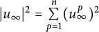 $|u_\infty |^2=\sum \limits _{p=1}^n(u_\infty ^p)^2$
. Then, by equation (3.1) and condition (4) of Theorem 2.8 for
 $\overline {w}$
, we easily see that there is a constant
 $C> 0$
such that
 $$ \begin{align} \begin{aligned} \frac{1}{C}\leq \frac{1-|u_\infty|}{1-\rho}\leq C. \end{aligned} \end{align} $$
Lemma 3.1 Let
 $$ \begin{align*} \begin{aligned} \Delta_M&=\sum\limits_{i,j=1}^m(\frac{(1-\rho^2)^2}{4}\delta_{ij}+O((1-\rho^2)^{4+a}))\frac{\partial^2 }{\partial x^i\partial x^j} \\& \quad +\sum\limits_{i=1}^m\frac{(m-2)}{2}((1-\rho^2)+O((1-\rho^2)^{3+a})x^i\frac{\partial }{\partial x^i}. \end{aligned} \end{align*} $$
For
 $0<s\leq m-1$
, there is a constant
 $\delta \in (0,1)$
such that
 $(1-\rho )^s$
is a superharmonic function of M at
 $B_1 \setminus B_\delta $
.
Proof Notice that
 $\Delta _{\mathbb {H}^m}=\frac {(1-\rho ^2)^2}{4}\Delta _0+\sum \limits _{i=1}^m\frac {(m-2)(1-\rho ^2)}{2}x^i\frac {\partial }{\partial x^i}$
, then
 $$\begin{align*}\Delta_M (1-\rho)^s=\Delta_{\mathbb{H}^m} (1-\rho)^s+O((1-\rho)^{s+2+a}). \end{align*}$$
According to Lemma 3.1 of [Reference Li and Tam16],
 $$ \begin{align*} \begin{aligned} \Delta_M (1-\rho)^s=\frac{s}{4}(1+\rho)(1-\rho)^{s+1}(-1-\frac{m-1}{\rho})+O((1-\rho)^{s+2+a}). \end{aligned} \end{align*} $$
Hence, there is a constant
 $\delta \in (0,1)$
such that
 $$ \begin{align*} \begin{aligned} \Delta_M (1-\rho)^s\leq 0 \text{ in } B_1 \setminus B_\delta. \end{aligned}\\[-33pt] \end{align*} $$
Similar to the proof of Lemmas 3.2 and 3.3 of [Reference Li and Tam16], we have
 $$ \begin{align*} \begin{aligned} d(u_\infty(x),\overline{w}(x))=O((1-\rho)^{m-1}\log(\frac{1}{1-\rho})) \end{aligned} \end{align*} $$
and
 $$ \begin{align*} \begin{aligned} |u_\infty(x)-\overline{w}(x)|=O((1-\rho)^{m}\log(\frac{1}{1-\rho})). \end{aligned} \end{align*} $$
From now on, since there is no ambiguity, we can simply denote
 $u_\infty $
by u.
Lemma 3.2 Assume the function
 $v(\rho ,\theta )$
on the
 $B^m$
satisfies
 $v=0$
at the boundary and for any
 $\varepsilon> 0$
, v is
 $C^{m-1,1-\varepsilon }$
up to the boundary. Also, for any
 $\varepsilon> 0$
,
 $ j\geq 0$
,
 $$ \begin{align*} \begin{aligned} |\nabla^j v|=O((1-\rho)^{m-j-\varepsilon}) \text{ as } \rho\rightarrow 1. \end{aligned} \end{align*} $$
Then, for any
 $s,j \geq 0$
, we have
 $$ \begin{align*} \begin{aligned} |\nabla^s_\theta\nabla^j v|=O((1-\rho)^{m-j-\varepsilon}) \text{ as } \rho\rightarrow 1. \end{aligned} \end{align*} $$
Proof Let
 $\varepsilon>0$
be fixed and define
 $k:=m-\varepsilon $
. Consequently, we have
 ${|v|=O((1-\rho )^k)}$
. Suppose
 $|\nabla v|=O((1-\rho )^{\overline {k}})$
. By Lemma 4.1 of [Reference Li and Tam16], it follows that
 $$ \begin{align} \begin{aligned} \sup\{ \overline{k}: \ |\nabla v|=O((1-\rho)^{\overline{k}})\}=k-1. \end{aligned} \end{align} $$
Let
 $d=1-\rho $
. Assume that
 $ |\partial _\theta v|=O((1-\rho )^{r})$
and define
 $$ \begin{align} \begin{aligned} s=\sup\{ r: \ |\partial_\theta v|=O((1-\rho)^{r})\}. \end{aligned} \end{align} $$
By the definition of supremum,
 $s-\delta <r\leq s, \forall \delta>0$
.
We aim to prove
 $s\geq k-\delta $
for all
 $\delta>0$
. We will proceed by contradiction. Assume
 $s< k-\delta _0$
for some
 $\delta _0>0$
, then it follows that
 $r< k-\delta _0$
.
Consider the case when
 $m=2$
, v has a Fourier series expansion
 $$ \begin{align*} \begin{aligned} v=\frac{a_0}{2}+\sum_{l=1}^\infty a_l\cos(l\theta)+ b_l\sin(l\theta), \end{aligned} \end{align*} $$
where the Fourier coefficients are given by
 $$ \begin{align*} \begin{aligned} a_l&=\frac{1}{\pi}\int_{-\pi}^\pi v(\rho,\theta)\cos l\theta \mathrm{d} \theta, l=0,1,2,\ldots\\b_l&=\frac{1}{\pi}\int_{-\pi}^\pi v(\rho,\theta)\sin l\theta \mathrm{d} \theta, l=1,2,\ldots \end{aligned} \end{align*} $$
Given the decay properties of v, we have
 $$ \begin{align*} \begin{aligned} a_l&=O((1-\rho)^k), l=0,1,2,\ldots\\b_l&=O((1-\rho)^k), l=1,2,\ldots \end{aligned} \end{align*} $$
Differentiating v with respect to
 $\theta $
, we obtain
 $$ \begin{align*} \begin{aligned} \frac{\partial v}{\partial \theta}=\sum_{l=1}^\infty -la_l\sin(l\theta)+l b_l\cos(l\theta). \end{aligned} \end{align*} $$
Since
 $ |\partial _\theta v|=O((1-\rho )^{r})$
, combining with (3.4) and
 $s<k-\delta _0$
, there must exist some
 $a_l$
or
 $b_l$
(without loss of generality, assume it is
 $a_l$
) such that
 $la_l=O((1-\rho )^{r})$
and
 $la_l\neq O((1-\rho )^{k})$
. This implies that l satisfies
 $l=O((1-\rho )^{r-k})$
. Therefore, v includes a term of the form
 $a_l \sin (h(\rho )(1-\rho )^{r-k}\theta )$
, where
 $h\in L^\infty (\overline {B})\cap C^\infty (B\setminus \{0\})$
. And then
 $\frac {\partial v}{\partial \rho }=O((1-\rho )^{r-1})$
. However,
 $r-1<k-\delta _0-1$
, which contradicts (3.3).
When
 $m\geq 3$
,
 $v=v(\rho ,\theta ^1,\ldots ,\theta ^{m-1})$
. Fix
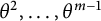 $\theta ^2,\ldots ,\theta ^{m-1}$
and regard v as a function of
 $\rho $
and
 $\theta ^1$
. Then, we can prove, similar to the case of
 $m=2$
, that
 $\frac {\partial v}{\partial \theta ^1}$
satisfies
 $ |\frac {\partial v}{\partial \theta ^1 }|=O((1-\rho )^{k-\delta })$
for any
 $\delta>0$
. Similarly, the partial derivative of v with respect to
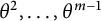 $\theta ^2,\ldots ,\theta ^{m-1}$
also has the same conclusion.
For any
 $s\geq 0$
,
 $g:=(1-\rho )^sv=O((1-\rho )^{m+s-\varepsilon })$
and
 $g\in C^{m+s-1,1-\varepsilon }(\overline {B^m}\setminus \{0\})$
. So we can use the method of Fourier expansion to prove
 $|\nabla ^s_\theta g|=O((1-\rho )^{m+s-\varepsilon })$
, that is,
 $|\nabla ^s_\theta v|=O((1-\rho )^{m-\varepsilon })$
.
Lemma 3.3 Let
 $\overline {w}$
be given by Theorem 2.8. Then, we have for any
 $\varepsilon> 0, j\geq 0$
that
 $$ \begin{align} \begin{aligned} |\nabla_0^j (u(x)-\overline{w}(x))|=O((1-\rho)^{m-j-\varepsilon}) \text{ as } \rho\rightarrow 1, \end{aligned} \end{align} $$
and for any
 $s,j \geq 0$
, we have
 $$ \begin{align} \begin{aligned} |\nabla^s_\theta\nabla_0^j (u(x)-\overline{w}(x))|=O((1-\rho)^{m-j-\varepsilon}) \text{ as } \rho\rightarrow 1. \end{aligned} \end{align} $$
Proof Let
 $v:=u-\overline {w}$
and define
 $d=1-\rho $
. According to Lemma 3.3 and Theorem 4.2 of [Reference Li and Tam16], we can assert that for any
 $\varepsilon>0$
and integers j satisfying
 $0\leq j\leq m-1$
,
 $|v|=O(d^{m-\varepsilon })$
and
 $|\nabla ^j_0 v|=O(d^{m-j-\varepsilon })$
. In our current analysis, instead of estimating
 $\Delta _0 v$
as was done in [Reference Li and Tam16], we need to focus on estimating
 $\sum \limits _{i,j=1}^m(\delta _{ij}+O((1-\rho ^2)^{2+a}))\frac {\partial ^2 v}{\partial x^i\partial x^j}$
. It is the second derivative part of
 $\Delta _M$
and thus it is an elliptic operator. Let
 $\phi _0,\overline {\phi }_1,\ldots , \overline {\phi }_m, \overline {\psi }_{m+1,1}$
in
 $C^{\infty }(\mathbb {S}^{m-1}, \mathbb {S}^{n-1})$
and
 $\overline {w}$
be given by Theorem 2.8. According to Theorem 2.8,
 $$ \begin{align} \begin{aligned} &O(d^{m+2}\log(-d))= \tau(\overline{w})\\& \quad =\sum\limits_{i,j=1}^m(\frac{(1-\rho^2)^2}{4}\delta_{ij}+O((1-\rho^2)^{4+a}))\frac{\partial^2 \overline{w}}{\partial x^i\partial x^j}\\& \qquad +\sum\limits_{i=1}^m\frac{(m-2)}{2}((1-\rho^2)+O((1-\rho^2)^{3+a})x^i\frac{\partial \overline{w}}{\partial x^i}\\& \qquad +\frac{(1-\rho^2)^2+O((1-\rho^2)^{4+a})}{2}(\frac{1}{1-|\overline{w}|^2}+O((1-|\overline{w}|^2)^{b+1})\\& \qquad \times(2 \langle \overline{w} , \nabla_0 \overline{w} \rangle \nabla_0\overline{w}-\langle \nabla_0 \overline{w}, \nabla_0 \overline{w} \rangle \overline{w}). \end{aligned} \end{align} $$
Let u be a harmonic map from M to N so that
 $u\in C^1$
as a map from
 $\overline {B}^m$
to
 $\overline {B}^n$
. Then,
 $$ \begin{align} \begin{aligned} \tau(u)=0. \end{aligned} \end{align} $$
Note that we have the following expression for
 $\overline {w:}$
 $$ \begin{align} \begin{aligned} \overline{w}=\phi_0+\sum\limits_{k=1}^{m} \overline{\phi}_kd(x)^k+\overline{\psi}_{m+1,1}d^{m+1} \log (-d). \end{aligned} \end{align} $$
For any
 $\varepsilon>0$
, since
 $u= \overline {w}+(u- \overline {w})$
, we get
 $$ \begin{align} \begin{aligned} u= \overline{w}+(u- \overline{w})=\phi_0+\phi_1 d+O(d^{2-\varepsilon}) . \end{aligned} \end{align} $$
Given that
 $|\phi _0|^2=1$
, we can derive
 $$ \begin{align*} \begin{aligned} |u|^2-1=2\langle\phi_0,\phi_1\rangle d+O(d^{2-\varepsilon}) \end{aligned} \end{align*} $$
and
 $$ \begin{align*} \begin{aligned} \frac{1-|u|^2}{1-\rho}=2\langle\phi_0,\phi_1\rangle +O(d^{1-\varepsilon}). \end{aligned} \end{align*} $$
Thus, we have
 $$ \begin{align} \begin{aligned} \frac{(1-\rho^2)^2}{2(1-|u|^2)}=\frac{(1+\rho)^2(1-\rho)}{4\langle\phi_0,\phi_1\rangle+O(d^{1-\varepsilon})}. \end{aligned} \end{align} $$
Additionally, consider the expression
 $$ \begin{align} \begin{aligned} &\frac{(1-\rho^2)^2+O((1-\rho^2)^{4+a})}{2}(\frac{1}{1-|u|^2}+O((1-|u|^2)^{b+1})\\& \quad =\frac{(1-\rho^2)^2}{2(1-|u|^2)}(1+O(1-\rho)). \end{aligned} \end{align} $$
By subtracting (3.7) from (3.8), we obtain
 $$ \begin{align} \begin{aligned} &O(d^{m+2}\log(-d))= \tau(u)-\tau(\overline{w})\\& \quad =\Delta_{M} v\\& \qquad + \frac{(1-\rho^2)^2}{2(1-|u|^2)}(1+O(1-\rho))\\& \qquad \times[ ( 2 \langle u , \nabla_0 u \rangle \nabla_0u-\langle \nabla_0 u, \nabla_0 u \rangle u )-(2 \langle \overline{w} , \nabla_0 \overline{w}\rangle \nabla_0\overline{w}-\langle \nabla_0 \overline{w}, \nabla_0 \overline{w} \rangle \overline{w})]\\& \qquad +(\frac{(1-\rho^2)^2}{2(1-|u|^2)}-\frac{(1-\rho^2)^2}{2(1-|\overline{w}|^2)}(1+O(1-\rho))\\& \qquad \times (2 \langle \overline{w} , \nabla_0 \overline{w}\rangle \nabla_0\overline{w}-\langle \nabla_0 \overline{w}, \nabla_0 \overline{w} \rangle \overline{w}). \end{aligned} \end{align} $$
The calculation of
 $ ( 2 \langle u , \nabla _0 u \rangle \nabla _0u-\langle \nabla _0 u, \nabla _0 u \rangle u )-(2 \langle \overline {w} , \nabla _0 \overline {w}\rangle \nabla _0\overline {w}-\langle \nabla _0 \overline {w}, \nabla _0 \overline {w} \rangle \overline {w})$
in a certain expansion process yields
 $$ \begin{align} \begin{aligned} & O(d^{m+2}\log(-d))\\& \quad =\Delta_{M} v+\frac{(1-\rho^2)^2}{2(1-|u|^2)}(1+O(1-\rho))[2(\langle u , \nabla_0 u \rangle \nabla_0v+(\langle v , \nabla_0 u \rangle\\& \qquad +\langle \overline{w} , \nabla_0 v\rangle)\nabla_0 \overline{w}) -(\langle\nabla_0 v,\nabla_0 u\rangle u+\langle\nabla_0 \overline{w},\nabla_0 v\rangle u+\langle\nabla_0 \overline{w},\nabla_0 \overline{w}\rangle v)]\\& \qquad +(\frac{(1-\rho^2)^2}{2(1-|u|^2)}-\frac{(1-\rho^2)^2}{2(1-|\overline{w}|^2)})(1+O(1-\rho))\\& \qquad \times(2 \langle \overline{w} , \nabla_0 \overline{w}\rangle \nabla_0\overline{w}-\langle \nabla_0 \overline{w}, \nabla_0 \overline{w} \rangle \overline{w}), \end{aligned} \end{align} $$
where
 $\Delta _M=\sum \limits _{i,j=1}^m(\frac {(1-\rho ^2)^2}{4}\delta _{ij}+O((1-\rho ^2)^{4+a}))\frac {\partial ^2 }{\partial x^i\partial x^j} +\sum \limits _{i=1}^m\frac {(m-2)}{2}((1-\rho ^2)+O((1-\rho ^2)^{3+a})x^i\frac {\partial }{\partial x^i}$
. For any
 $l>0$
, given that
 $|\nabla _0 v|=O((1-\rho )^{m-\varepsilon -1})$
, we can deduce that
 $\sum \limits _{i,j=1}^m(\delta _{ij}+O((1-\rho ^2)^{2+a}))\frac {\partial ^2 }{\partial x^i\partial x^j}((1-\rho )^lv)=O((1-\rho )^{m+l-\varepsilon -2})$
and must be
 $C^{m+l-3,1-\varepsilon }$
up to the boundary. Together with the fact that
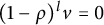 $(1-\rho )^lv=0$
at the boundary, this implies that
 $(1-\rho )^lv$
is
 $C^{m+l-1,1-\varepsilon }$
up to the boundary. In particular,
 $|\nabla ^{m+l-1}((1-\rho )^lv)|=O((1-\rho )^{1-\varepsilon })$
. Therefore, we have
 $$ \begin{align*} \begin{aligned} |\nabla_0^{m+l-1}v|=O((1-\rho)^{1-\varepsilon-l}), \end{aligned} \end{align*} $$
and subsequently,
 $$ \begin{align*} \begin{aligned} |\nabla^j_0 v|=O(d^{m-j-\varepsilon}), \forall \varepsilon>0, j\geq 0. \end{aligned} \end{align*} $$
Theorem 3.4 Let M and N be asymptotically hyperbolic spaces with metrics (1.2) and (1.3), respectively, in the Poincaré disk model. Let u be a harmonic map from M to N so that
 $u\in C^1$
as a map from
 $\overline {B^m}$
to
 $\overline {B^n}$
. Suppose that the boundary map
 $\phi _0$
of u, when restricted to
 $\mathbb {S}^{m-1}$
, is in
 $C^{\infty }(\mathbb {S}^{m-1}, \mathbb {S}^{n-1})$
, and has nowhere-vanishing energy density with respect to the standard metrics. Then,
 $u\in C^{m-1,\alpha }(\overline {B^m},\overline {B^n})$
for all
 $0<\alpha <1$
.
Proof Notice that
 $u-\overline {w}=0$
on
 $\partial B^m$
. According to Lemma 3.3 and Theorem 4.2 of [Reference Li and Tam16],
 $u-\overline {w}\in C^{m-1,\alpha }(\overline {B^m},\overline {B^n})$
and then
 $u\in C^{m-1,\alpha }(\overline {B^m},\overline {B^n})$
for all
 $0<\alpha <1$
.
4 Optimal regularity near the boundary
4.1 Equations of
$v=u-\overline {w}$

First, note the following expression for
 $\overline {w}$
:
 $$ \begin{align} \begin{aligned} \overline{w}=\phi_0+\sum\limits_{k=1}^{m} \overline{\phi}_kd(x)^k+\overline{\psi}_{m+1,1}d^{m+1} \log (-d). \end{aligned} \end{align} $$
Differentiating
 $\overline {w}$
with respect to
 $x^i(i=1,\ldots ,m)$
, we obtain
 $$ \begin{align} \begin{aligned} \frac{\partial \overline{w}}{\partial x^i}=\frac{\partial \phi_0}{\partial x^i}+\phi_1\frac{x^i}{\rho}+O(d),i=1,\ldots,m. \end{aligned} \end{align} $$
It follows that for any
 $\varepsilon>0$
,
 $$ \begin{align} \begin{aligned} u&=\overline{w}+(u-\overline{w})=\phi_0+\phi_1 d+O(d^{2-\varepsilon}) ,\\\frac{\partial u}{\partial x^i}&= \frac{\partial \overline{w}}{\partial x^i}+\frac{\partial (u-\overline{w})}{\partial x^i} =\frac{\partial \phi_0}{\partial x^i}+\phi_1\frac{x^i}{\rho}+O(d^{1-\varepsilon}),i=1,\ldots,m. \end{aligned} \end{align} $$
Taking into account equation (4.3) and the fact that
 $|\phi _0|^2\equiv 1$
, we can deduce that the inner product
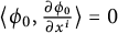 $\langle \phi _0, \frac {\partial \phi _0}{\partial x^i}\rangle =0$
for all
 $i=1,\ldots , m$
. Taking into account (3) of Theorem 2.8, we see that
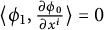 $\langle \phi _1, \frac {\partial \phi _0}{\partial x^i}\rangle =0$
for all
 $i=1,\ldots , m$
and then
 $$ \begin{align} \begin{aligned} 2 \langle u , \nabla_0 u\rangle \nabla_0 &=2 \sum\limits_{i=1}^m(\langle \phi _0, \phi_1\frac{x^i}{\rho}\rangle+O(d^{1-\varepsilon}) ) \frac{\partial}{\partial x^i}.\end{aligned} \end{align} $$
We can apply (3.11) and (4.4) to deduce
 $$ \begin{align} \begin{aligned} \frac{(1-\rho^2)^2}{(1-|u|^2)} \langle u , \nabla_0 u\rangle \nabla_0 &=\frac{(1+\rho)^2(1-\rho)}{2\langle\phi_0,\phi_1\rangle+O(d^{1-\varepsilon})} \sum\limits_{i=1}^m(\langle \phi _0, \phi_1\frac{x^i}{\rho}\rangle+O(d^{1-\varepsilon}) ) \frac{\partial}{\partial x^i}\\&=[\frac{(1+\rho)(1-\rho^2)}{2\rho}+O(d^{2-\varepsilon}) ]\sum\limits_{i=1}^mx^i \frac{\partial}{\partial x^i}\\&=[(1-\rho^2) +O(d^{2-\varepsilon})]\sum\limits_{i=1}^mx^i \frac{\partial}{\partial x^i}. \end{aligned} \end{align} $$
Define linear operator
 $$ \begin{align} \begin{aligned} L&:=\Delta_{\mathit{H}}+(1-\rho^2) \sum\limits_{i=1}^mx^i \frac{\partial}{\partial x^i}\\&=\frac{(1-\rho^2)^2}{4}\Delta_0+\sum\limits_{i=1}^m\frac{m(1-\rho^2)}{2}x^i\frac{\partial }{\partial x^i}. \end{aligned} \end{align} $$
The right side of equation (3.14) can be written in two parts. The first part is
 $$ \begin{align*} \begin{aligned} &\Delta_{M} v+ \frac{(1-\rho^2)^2}{2(1-|u|^2)}(1+O(1-\rho))[2(\langle u , \nabla_0 u \rangle \nabla_0v+(\langle v , \nabla_0 u \rangle+\langle \overline{w} , \nabla_0 v\rangle)\nabla_0 \overline{w})\\& \qquad -(\langle\nabla_0 v,\nabla_0 u\rangle u+\langle\nabla_0 \overline{w},\nabla_0 v\rangle u+\langle\nabla_0 \overline{w},\nabla_0 \overline{w}\rangle v)]\\& \quad =Lv+\frac{(1-\rho^2)^2}{2(1-|u|^2)}[2 \langle \overline{w} , \nabla_0 v\rangle\nabla_0 \overline{w} -(\langle\nabla_0 v,\nabla_0 u\rangle u+\langle\nabla_0 \overline{w},\nabla_0 v\rangle u)]\\& \qquad +O(d^{3})|\nabla^2_0 v|+O(d^{2-\varepsilon})|\nabla_0 v|+O(d)|v|. \end{aligned} \end{align*} $$
In the
 $ m $
-dimensional spherical coordinates
 $(\rho , \theta ^1, \theta ^2, \ldots , \theta ^{m-1})$
, the expression for the gradient operator
 $ \nabla _0$
is
 $$ \begin{align} \begin{aligned} \nabla_0 = \frac{\partial}{\partial \rho} \mathbf{e}_\rho + \frac{1}{\rho} \sum_{k=1}^{m-1} \left( \frac{1}{\prod_{j=1}^{k-1} \sin \theta^j} \frac{\partial}{\partial \theta^k} \mathbf{e}_{\theta^k} \right), \end{aligned} \end{align} $$
where
 $ \mathbf {e}_\rho $
is the radial unit vector and
 $\mathbf {e}_{\theta ^k} $
are the angular unit vectors corresponding to the coordinates
 $\theta ^k $
.
 $ \prod _{j=1}^{k-1} \sin \theta ^j $
denotes the product of
 $ \sin \theta ^j $
from
 $ j=1 $
to
 $ k-1 $
, with the convention that
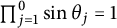 $ \prod _{j=1}^0 \sin \theta _j = 1 $
. Then, (4.1)–(4.3) imply
 $$ \begin{align*} \begin{aligned} &2 \langle {\overline{w}}, \nabla_0 v\rangle\nabla_0 {\overline{w} }-(\langle\nabla_0 v,\nabla_0 u\rangle u+\langle\nabla_0 {\overline{w}},\nabla_0 v\rangle u).\\& \quad =2\langle \phi_0 , \partial_\rho v\rangle\phi_1 -2\langle \partial_\rho v,\phi_1 \rangle \phi_0+O(d^{1-\varepsilon}) |\partial_\rho v|+O(1) |\nabla_\theta v|. \end{aligned} \end{align*} $$
Since (3) of Theorem 2.8,
 $\langle \phi _0 , \partial _\rho v\rangle \phi _1 =\langle \partial _\rho v,\phi _1 \rangle \phi _0$
. And then
 $$ \begin{align} \begin{aligned} &\Delta_{M} v+ \frac{(1-\rho^2)^2}{2(1-|u|^2)}(1+O(1-\rho))[2(\langle u , \nabla_0 u \rangle \nabla_0v+(\langle v , \nabla_0 u \rangle\\& \qquad +\langle \overline{w} , \nabla_0 v\rangle)\nabla_0 \overline{w}) -(\langle\nabla_0 v,\nabla_0 u\rangle u+\langle\nabla_0 \overline{w},\nabla_0 v\rangle u+\langle\nabla_0 \overline{w},\nabla_0 \overline{w}\rangle v)]\\& \quad =Lv+O(d^{3})|\nabla^2_0 v|+O(d^{2-\varepsilon})|\nabla_0 v|+O(d)(|v|+|\nabla_\theta v|). \end{aligned} \end{align} $$
The second part of (3.14) is
 $$ \begin{align} \begin{aligned} & (\frac{(1-\rho^2)^2}{2(1-|u|^2)}-\frac{(1-\rho^2)^2}{2(1-|\overline{w}|^2)})(1+O(1-\rho))\\& \qquad \times(2 \langle \overline{w} , \nabla_0 \overline{w}\rangle \nabla_0\overline{w}-\langle \nabla_0 \overline{w}, \nabla_0 \overline{w} \rangle \overline{w})\\& \quad =\frac{(2-m)(1+\rho)^2}{4}\langle v , \phi_0\rangle \phi_0+O(d^{1-\varepsilon}) v. \end{aligned} \end{align} $$
In fact, we can calculate
 $$ \begin{align*} \begin{aligned} \frac{(1-\rho^2)^2}{2(1-|u|^2)}-\frac{(1-\rho^2)^2}{2(1-|\overline{w}|^2)}&= \frac{(1-\rho^2)^2(u+\overline{w})v}{2(1-|u|^2)(1-|\overline{w}|^2)}\\&=\frac{(1-\rho^2)^2\langle \phi_0 , v\rangle }{(1-|u|^2)(1-|\overline{w}|^2)}+O(d^{1-\varepsilon})v. \end{aligned} \end{align*} $$
Since
 $\langle \phi _0,\phi _0\rangle \equiv 1$
,
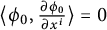 $\langle \phi _0,\frac {\partial \phi _0}{\partial x^i}\rangle =0$
, for any
 $i=1, \ldots ,m$
. Equations (2.41), (4.1), and (4.2) imply that
 $$ \begin{align*} \begin{aligned} &2 \langle \overline{w} , \nabla_0 \overline{w}\rangle \nabla_0\overline{w}-\langle \nabla_0 \overline{w}, \nabla_0 \overline{w} \rangle \overline{w}\\& \quad =2 \langle \phi _0, \phi_1 \rangle \phi_1-\langle \nabla_0 \phi _0, \nabla_0 \phi _0 \rangle \phi _0-\langle \phi _1, \phi_1 \rangle \phi_0+O(d)\\& \quad =(2-m)A_{1,0}^2\phi_0+O(d), \end{aligned} \end{align*} $$
where
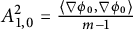 $A_{1,0}^2=\frac {\langle \nabla \phi _0,\nabla \phi _0\rangle }{m-1}$
.
We conclude from (3.14), (4.8), and (4.9) that
 $$ \begin{align*} \begin{aligned} &Lv-\frac{(m-2)(1+\rho)^2}{4}\langle v , \phi_0\rangle\phi_0\\& \quad =O(d^{3})|\nabla^2_0 v|+O(d^{2-\varepsilon})|\nabla_0 v|+O(d)(|v|+|\nabla_\theta v|)+O(d^{m+2}\log(-d)). \end{aligned} \end{align*} $$
Notice that
 $\frac {(1+\rho )^2}{4}-1=\frac {(\rho +3)(\rho -1)}{4}$
. Then, v satisfies
 $$ \begin{align} \begin{aligned} &Lv-(m-2)\langle v , \phi_0\rangle\phi_0\\& \quad =O(d^{3})|\nabla^2_0 v|+O(d^{2-\varepsilon})|\nabla_0 v|+O(d)(|v|+|\nabla_\theta v|)+O(d^{m+2}\log(-d)). \end{aligned} \end{align} $$
4.2 Estimate of
$\langle u-\overline {w}, \phi _0\rangle $
and
$u-\overline {w}$


When
 $m\geq 3$
, we need to deal with
 $(m-2)\langle v , \phi _0\rangle \phi _0$
.
Lemma 4.1 Let u be a harmonic map from M to N so that
 $u\in C^1$
as a map from
 $\overline {B^m}$
to
 $\overline {B^n}$
. Suppose that the boundary map
 $\phi _0$
of u, when restricted to
 $\mathbb {S}^{m-1}$
, is in
 $C^{\infty }(\mathbb {S}^{m-1}, \mathbb {S}^{n-1})$
, and has nowhere-vanishing energy density with respect to the standard metrics. Let
 $\phi _0, \overline {\phi }_1, \ldots , \overline {\phi }_m, \overline {\psi }_{m+1,1}$
in
 $C^{\infty }(\mathbb {S}^{m-1}, \mathbb {S}^{n-1})$
and
 $\overline {w}$
be given by Theorem 2.8. Then,
 $\langle u-\overline {w},\phi _0\rangle =O((1-\rho )^{m+1+\varepsilon _0})$
and
 $ u-\overline {w}=O((1-\rho )^{m+1})$
, where
 $\varepsilon _0=\frac {(m+1)+\sqrt {(m+1)^2+4(m-2)}}{2}-m-1$
. In addition, for any
 $\varepsilon> 0, j\geq 0$
,
 $$ \begin{align} \begin{aligned} |\nabla_0^j \langle u-\overline{w}, \phi_0\rangle|=O((1-\rho)^{m+1+\varepsilon_0-j-\varepsilon}) \text{ as } \rho\rightarrow 1^{-}, \end{aligned} \end{align} $$
and for any
 $s,j \geq 0$
, we have
 $$ \begin{align} \begin{aligned} |\nabla^s_\theta\nabla_0^j \langle u-\overline{w}, \phi_0\rangle|=O((1-\rho)^{m+1+\varepsilon_0-j-\varepsilon}) \text{ as } \rho\rightarrow 1^{-}. \end{aligned} \end{align} $$
Proof Set
 $v:=u-\overline {w}$
. Multiplying (4.10) by
 $\phi _0$
, we have
 $$ \begin{align} \begin{aligned} &L\langle v , \phi_0\rangle-(m-2)\langle v , \phi_0\rangle\\& \quad =O(d^{3})|\nabla^2_0 v|+O(d^{2-\varepsilon})|\nabla_0 v|+O(d)(|v|+|\nabla_\theta v|)+O(d^{m+2}\log(-d)). \end{aligned} \end{align} $$
Define
 $v_0:=\langle v,\phi _0 \rangle $
. By Proposition 3.3, for any
 $\varepsilon>0$
and non-negative integers
 $j, s$
, we have
 $|\nabla _\theta ^s\nabla ^j v_0|=O((1-\rho )^{m-j-\varepsilon })$
.
In the
 $ m $
-dimensional spherical coordinates
 $(\rho , \theta ^1, \theta ^2, \ldots , \theta ^{m-1})$
, the expression for the gradient operator
 $ \nabla _0$
is (4.7) and the expression for the Laplace operator
 $ \Delta _0$
are
 $$ \begin{align} \begin{aligned} \Delta_0 = \frac{\partial^2}{\partial \rho^2}+\frac{m-1}{\rho}\frac{\partial}{\partial \rho}+\frac{1}{\rho^2}\Delta_{\mathbb{S}^{m-1}}, \end{aligned} \end{align} $$
where
 $\Delta _{\mathbb {S}^{m - 1}}$
is the Laplace operator on the
 $(m - 1)$
-dimensional sphere.
Hence, by (4.13), along the direction
 $\rho $
,
 $v_0:=\langle v , \phi _0\rangle $
satisfies the ODEs
 $$ \begin{align} \begin{aligned} \frac{(1-\rho^2)^2}{4}\frac{\partial ^2v_0}{\partial \rho^2}+\frac{m(1-\rho^2)}{2}\rho\frac{\partial v_0}{\partial \rho}-(m-2)v_0=O(d^{m+1-2\varepsilon}). \end{aligned} \end{align} $$
Define
 $r:=\frac {1-\rho }{1+\rho }$
. We compute
 $$ \begin{align*} \begin{aligned} \frac{\partial v_0}{\partial \rho}&=\frac{\partial v_0}{\partial r}\frac{\partial r }{\partial \rho}=-\frac{2}{(1+\rho)^2}\frac{\partial v_0}{\partial r}=-\frac{(1+r)^2}{2}\frac{\partial v_0}{\partial r},\\\frac{\partial ^2v_0}{\partial \rho^2}&=\frac{\partial(\frac{\partial v_0}{\partial \rho})}{\partial r}\frac{\partial r }{\partial \rho}=\frac{(1+r)^4}{4}\frac{\partial^2 v_0}{\partial r^2}+\frac{(1+r)^3}{2}\frac{\partial v_0}{\partial r}. \end{aligned} \end{align*} $$
Based on the above calculations, we can derive
 $$ \begin{align} \begin{aligned} r^2\frac{\partial ^2v_0}{\partial r^2}-mr\frac{\partial v_0}{\partial r}-(m-2)v_0=:\eta=O(r^{m+1-2\varepsilon}). \end{aligned} \end{align} $$
Let
 $t=\ln r$
and then
 $r=e^t$
. We proceed to compute the derivatives of
 $v_0$
with respect to r in terms of t
 $$ \begin{align} \begin{aligned} \frac{\partial v_0}{\partial r}&=\frac{\partial v_0}{\partial t}\frac{\partial t}{\partial r}=e^{-t}\frac{\partial v_0}{\partial t},\\\frac{\partial^2 v_0}{\partial r^2}&=\frac{\partial (\frac{\partial v_0}{\partial r})}{\partial t}\frac{\partial t}{\partial r}=e^{-2t}\frac{\partial^2 v_0}{\partial t^2}-e^{-2t}\frac{\partial v_0}{\partial t}. \end{aligned} \end{align} $$
Substituting (4.17) into (4.16), we obtain the following second-order linear ordinary differential equation:
 $$ \begin{align} \begin{aligned} \frac{\partial ^2v_0}{\partial t^2}-(m+1)\frac{\partial v_0}{\partial t}-(m-2)v_0=\eta. \end{aligned} \end{align} $$
It has two characteristic roots
 $$ \begin{align*} \begin{aligned} \mu_1=\frac{(m+1)-\sqrt{(m+1)^2+4(m-2)}}{2}, \ \mu_2=\frac{(m+1)+\sqrt{(m+1)^2+4(m-2)}}{2}. \end{aligned} \end{align*} $$
We have an explicit formula for
 $v_0$
,
 $$ \begin{align*} \begin{aligned} v_0=C_1(\theta) e^{\mu_1t}+C_2(\theta) e^{\mu_2t}+G_0(\eta), \end{aligned} \end{align*} $$
where
 $$ \begin{align*} \begin{aligned} G_0(\eta)=\frac{1}{\mu_2-\mu_1}[ e^{\mu_2t}\int_{t_1}^te^{-\mu_2\tau}\eta(\tau,\theta)\mathrm{d} \tau-e^{\mu_1t}\int_{-\infty}^te^{-\mu_1\tau}\eta(\tau,\theta)\mathrm{d} \tau], t_1\in (-\infty,t). \end{aligned} \end{align*} $$
Note that
 $r=e^t$
.
 $$ \begin{align*} \begin{aligned} v_0=C_1(\theta) r^{\mu_1}+C_2(\theta) r^{\mu_2}+G_0(\eta) \end{aligned} \end{align*} $$
with
 $$ \begin{align*} \begin{aligned} G_0(\eta)=\frac{1}{\mu_2-\mu_1}[ r^{\mu_2}\int_{e^{t_1}}^rs^{-1-\mu_2}\eta(s,\theta)\mathrm{d} s-r^{\mu_1}\int_0^rs^{-1-\mu_1}\eta(s,\theta)\mathrm{d} s]. \end{aligned} \end{align*} $$
From (4.16), there exists a positive number
 $C>0$
such that
 $|\eta (s,\theta )|\leq Cs^{m+1-2\varepsilon }$
. Therefore,
 $$ \begin{align*} \begin{aligned} |G_0(\eta)|\leq C r^{m+1-2\varepsilon}+\widetilde{C} r^{\mu_2}. \end{aligned} \end{align*} $$
Since we have known
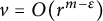 $v= O(r^{m -\varepsilon })$
,
 $C_1=0$
. So
 $$ \begin{align} \begin{aligned} v_0=C_2(\theta) r^{\mu_2}+G_0(\eta). \end{aligned} \end{align} $$
In view of
 $G_0(\eta )=O(r^{m+1-2\varepsilon })$
, we have
 $v_0=O(r^{m+1-2\varepsilon })$
.
Owing to (4.10) and (4.19), v satisfies equation
 $$\begin{align*}Lv=\frac{(1-\rho^2)^2}{4}\Delta_0 v+\sum\limits_{i=1}^m\frac{m(1-\rho^2)}{2}x^i\frac{\partial v}{\partial x^i}=O(d^{m+1-2\varepsilon}). \end{align*}$$
By Proposition 3.3, v satisfies the ODEs
 $$ \begin{align} \begin{aligned} \frac{(1-\rho^2)^2}{4}\frac{\partial ^2v}{\partial \rho^2}+\frac{m(1-\rho^2)}{2}\rho\frac{\partial v}{\partial \rho}=O(d^{m+1-2\varepsilon}). \end{aligned} \end{align} $$
Notice that
 $r=\frac {1-\rho }{1+\rho }$
, v satisfies
 $$ \begin{align} \begin{aligned} r^2\frac{\partial ^2v}{\partial r^2}-mr\frac{\partial v}{\partial r}=:\overline{\eta}=O(r^{m+1-2\varepsilon}). \end{aligned} \end{align} $$
Let
 $t=\ln r$
and then
 $r=e^t$
. We compute
 $$ \begin{align} \begin{aligned} \frac{\partial ^2v}{\partial t^2}-(m+1)\frac{\partial v}{\partial t}=\overline{\eta}. \end{aligned} \end{align} $$
It has two characteristic roots
 $$ \begin{align*} \begin{aligned} \overline{\mu}_1=0, \ \overline{\mu}_2=m+1. \end{aligned} \end{align*} $$
We have an explicit formula for v,
 $$ \begin{align*} \begin{aligned} v=\overline{C}_1(\theta) e^{\overline{\mu}_1t}+\overline{C}_2(\theta) e^{\overline{\mu}_2t}+\overline{G}_0(\eta), \end{aligned} \end{align*} $$
where
 $$ \begin{align*} \begin{aligned} \overline{G}_0(\eta)=\frac{1}{\overline{\mu}_2-\overline{\mu}_1}[ e^{\overline{\mu}_2t}\int_{\overline{t}_1}^te^{-\overline{\mu}_2\tau}\overline{\eta}(\tau,\theta)\mathrm{d} \tau-e^{\overline{\mu}_1t}\int_{-\infty}^te^{-\overline{\mu}_1t}\overline{\eta}(\tau,\theta)\mathrm{d} \tau], \overline{t}_1\in (-\infty,t). \end{aligned} \end{align*} $$
Notice that
 $r=e^t$
,
 $$ \begin{align*} \begin{aligned} v=\overline{C}_1(\theta) r^{\overline{\mu}_1}+\overline{C}_2(\theta) r^{\overline{\mu}_2}+\overline{G}_0(\eta), \end{aligned} \end{align*} $$
with
 $$ \begin{align*} \begin{aligned} \overline{ G}_0(\eta)=\frac{1}{\overline{\mu}_2-\overline{\mu}_1}[ r^{\overline{\mu}_2}\int_{e^{\overline{t}_1}}^rs^{-1-\mu_2}\overline{\eta}(s,\theta)\mathrm{d} s-r^{\overline{\mu}_1}\int_0^rs^{-1-\overline{\mu}_1}\overline{\eta}(s,\theta)\mathrm{d} s]. \end{aligned} \end{align*} $$
From (4.16), there exists a positive number
 $C>0$
such that
 $|\overline {\eta }(s,\theta )|\leq Cs^{m+1-2\varepsilon }$
. Therefore,
 $$ \begin{align*} \begin{aligned} |\overline{G}_0(\eta)|\leq C r^{m+1-2\varepsilon}+\hat{C} r^{\overline{\mu}_2}. \end{aligned} \end{align*} $$
Since we have known
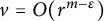 $v= O(r^{m-\varepsilon })$
,
 $\overline {C}_1=0$
. So
 $$ \begin{align} \begin{aligned} v=(\overline{C}_2\theta) r^{\overline{\mu}_2}+\overline{G}_0(\eta). \end{aligned} \end{align} $$
In view of
 $\overline {G}_0(\eta )=O(r^{m+1-2\varepsilon })$
, we have
 $v=O(r^{m+1-2\varepsilon })$
.
Repeating the process above, we can get
 $\langle v, \phi _0\rangle =O(r^{\min \{\mu _2,m+2-3\varepsilon \}})=O(r^{\mu _2}), (\mu _2=\frac {(m+1)+\sqrt {(m+1)^2+4(m-2)}}{2})$
and
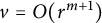 $v=O(r^{m+1}) $
.
According to (4.13),
 $v_0=\langle v,\phi _0 \rangle $
satisfies the conditions of Lemma 4.1 of [Reference Li and Tam16] if the general elliptic operator is substituted for
 $\Delta _0$
. Similar to the proof of Proposition 3.3 (Replace m in Proposition 3.3 with
 $m+1+\varepsilon _0$
.), for any
 $\varepsilon>0$
and non-negative integers
 $j, s$
, we have
 $|\nabla _\theta ^s\nabla ^j v_0|=O((1-\rho )^{m+1+\varepsilon _0-j-\varepsilon })$
.
4.3 The coefficient function
$\overline {\phi }_{m+1}$
and the rest of the proof

The next step in the proof of Theorem 1.1 is to find
 $W_{m+1}=\overline {w}+\overline {\phi }_{m+1}d^{m+1}$
, where
 $\overline {w}$
is given by Theorem 2.8 such that
 $u-W_{m+1}=o(d^{m+1})$
.
We have already proved
 $u-\overline {w}=O(d^{m+1})$
in Lemma 4.1, but since we have reached the conclusion by solving ordinary differential equations, the coefficient
 $\frac {u-\overline {w}}{d^{m+1}}$
is not yet certain. Therefore, the following lemma proves this coefficient by the convergence method.
Define
 $$ \begin{align} \begin{aligned} c(\rho, \theta)=\frac{u-\overline{w}}{d^{m+1}}(\rho, \theta). \end{aligned} \end{align} $$
Lemma 4.2 Let u be a harmonic map from M to N so that
 $u\in C^1$
as a map from
 $\overline {B^m}$
to
 $\overline {B^n}$
. Suppose that the boundary map
 $\phi _0$
of u, when restricted to
 $\mathbb {S}^{m-1}$
, is in
 $C^{\infty }(\mathbb {S}^{m-1}, \mathbb {S}^{n-1})$
, and has nowhere-vanishing energy density with respect to the standard metrics. Let
 $\phi _0,\overline {\phi }_1, \ldots , \overline {\phi }_m, \overline {\psi }_{m+1,1}$
in
 $C^{\infty }(\mathbb {S}^{m-1}, \mathbb {S}^{n-1})$
and
 $\overline {w}$
be given by Theorem 2.8. Let c be defined by (4.24). Then, there exists
 $\overline {\phi }_{m+1}\in C^\infty ( \mathbb {S}^{m-1};\mathbb {S}^{n-1})$
such that c converges to
 $\overline {\phi }_{m+1}$
in
 $C^j(\mathbb {S}^{m-1};\mathbb {S}^{n-1})$
for all
 $j\geq 0$
as
 $\rho \rightarrow 1$
, and for any
 $s\geq 0$
,
 $$ \begin{align} \begin{aligned} |\nabla^s_\theta(c-\overline{\phi}_{m+1})|\leq C(1-\rho)^{1-\varepsilon}, \end{aligned} \end{align} $$
where
 $\varepsilon $
can take any real number in
 $(0,1)$
.
Proof Set
 $v:=u-\overline {w}$
. By Proposition 3.3 and Lemma 4.1, we know for any
 $\varepsilon>0$
and non-negative integers
 $j,s$
,
 $|\nabla ^j\nabla ^s_\theta v|=O((1-\rho )^{m+1-j-\varepsilon })$
.
Define function
 $\varphi :=\nabla _\theta ^s v$
and
 $\varphi _0:=\nabla _\theta ^s\langle v, \phi _0\rangle $
. Differentiating (4.13) with respect to
 $\theta s$
times, we know
 $$ \begin{align} \begin{aligned} &L\varphi_0-(m-2)\varphi_0=O((1-\rho)^{m+2-\varepsilon}). \end{aligned} \end{align} $$
Set
 $r=\frac {1-\rho }{1+\rho }$
and
 $\mu _2=\frac {(m+1)+\sqrt {(m+1)^2+4(m-2)}}{2}$
. So for any fixed
 $\theta _0\in \mathbb {S}^{m-1}$
, we have
 $$ \begin{align*} \begin{aligned} r^2\frac{\partial ^2\varphi_0(\theta_0,r)}{\partial r^2}-mr\frac{\partial \varphi_0(\theta_0,r)}{\partial r}-(m-2)\varphi_0=O(r^{m+2-\varepsilon}). \end{aligned} \end{align*} $$
Introducing
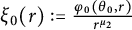 $\xi _0(r):=\frac {\varphi _0(\theta _0,r)}{r^{\mu _2}}$
, we have
 $$ \begin{align*} \begin{aligned} & r^{\mu_2+2}\frac{\partial^2 \xi_0}{\partial r^2}+(2\mu_2-m)r^{\mu_2+1}\frac{\partial \xi_0}{\partial r}\\& \quad =r^2\frac{\partial^2 \varphi_0}{\partial r^2}-mr \frac{\partial \varphi_0}{\partial r}-\mu_2(\mu_2-m-1)\varphi_0=O(r^{m+2-\varepsilon}),\\& \qquad (r^{\mu_2+2}\xi_0^{'}(r))^{'} +(\mu_2-m-2)r^{\mu_2+1}\xi_0^{'}(r)=O(r^{m+2-\varepsilon}), \end{aligned} \end{align*} $$
where we have used that
 $\mu _2$
is a solution of
 $\mu _2^2-(m+1)\mu _2-(m-2)=0$
.
Set
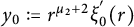 $y_0:=r^{\mu _2+2}\xi _0^{'}(r)$
and notice that
 $\mu _2<m+2$
. Then,
 $y_0$
satisfies the following ODE and
 $$ \begin{align*} \begin{aligned} ry_0^{'}(r)+(\mu_2-m-2)y_0=:\pi_0=O(r^{m+3-\varepsilon}) \end{aligned} \end{align*} $$
has solution
 $$ \begin{align*} \begin{aligned} y_0(r)=r^{m+2-\mu_2}(\int_{r_0}^r \pi_0(R)R^{\mu_2-m-3}\mathrm{d} R+\widetilde{C}), \end{aligned} \end{align*} $$
where
 $r_0\in (0,r)$
. Since
 $y_0=O(r^{\mu _2+1-\varepsilon })$
,
 $\widetilde {C}=0,$
and
 $y_0=O(r^{m+3-\varepsilon })$
. Therefore,
 $\xi _0^{'}(r)=O(r^{m+1-\mu _2-\varepsilon })$
, which gives
 $\xi _0(r)=O(r^{m+2-\mu _2-\varepsilon })$
and
 $\varphi _0=O(r^{m+2-\varepsilon })$
.
Differentiating (4.10) with respect to
 $\theta s$
times, we have
 $$ \begin{align*} \begin{aligned} L\varphi=\frac{(1-\rho^2)^2}{4}\Delta_0\varphi+\sum\limits_{i=1}^m\frac{m(1-\rho^2)}{2}x^i\frac{\partial \varphi}{\partial x^i}=O((1-\rho)^{m+2-\varepsilon}). \end{aligned} \end{align*} $$
Similar to the estimate of
 $\varphi _0$
, we can get
 $$ \begin{align*} \begin{aligned} r^2\frac{\partial ^2\varphi(\theta_0,r)}{\partial r^2}-mr\frac{\partial \varphi(\theta_0,r)}{\partial r}=O(r^{m+2-\varepsilon}). \end{aligned} \end{align*} $$
Introducing
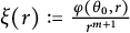 $\xi (r):=\frac {\varphi (\theta _0,r)}{r^{m+1}}$
, we have
 $$ \begin{align*} \begin{aligned} r^{m+3}\frac{\partial^2 \xi}{\partial r^2}+(m+2)r^{m+2}\frac{\partial \xi}{\partial r}&=r^2\frac{\partial^2 \varphi}{\partial r^2}-mr \frac{\partial \varphi}{\partial r}=O(r^{m+2-\varepsilon}),\\(r^{m+3}\xi^{'}(r))^{'} -r^{m+2}\xi^{'}(r)&=O(r^{m+2-\varepsilon}). \end{aligned} \end{align*} $$
Set
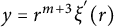 $y=r^{m+3}\xi ^{'}(r)$
, then
 $$ \begin{align*} \begin{aligned} ry^{'}(r)-y=:\pi=O(r^{m+3-\varepsilon}) \end{aligned} \end{align*} $$
has solution
 $$ \begin{align*} \begin{aligned} y(r)=r(\int_0^r R^{-2}\pi(R)\mathrm{d} R+\widetilde{C}). \end{aligned} \end{align*} $$
Since
 $y=O(r^{m+2-\varepsilon })$
,
 $\widetilde {C}=0,$
and
 $y=O(r^{m+3-\varepsilon })$
. Therefore,
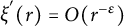 $\xi ^{'}(r)=O(r^{-\varepsilon })$
, which gives
 $$ \begin{align*} \begin{aligned} |\frac{\nabla^s_\theta v(\theta_0,r)}{r^{m+1}}-\frac{\nabla^s_\theta v(\theta_0,\overline{r})}{\overline{r}^{m+1}}|=|\xi(r)-\xi(\overline{r})|\leq C|r^{1-\varepsilon}-\overline{r}^{1-\varepsilon}| \end{aligned} \end{align*} $$
and
 $$ \begin{align*} \begin{aligned} |\nabla^s_\theta(\frac{ v(\theta_0,\rho)}{(1-\rho)^{m+1}}-\frac{ v(\theta_0,\overline{\rho})}{(1-\overline{\rho})^{m+1}})|\leq C|(1-\rho)^{1-\varepsilon}-(1-\overline{\rho})^{1-\varepsilon}|. \end{aligned} \end{align*} $$
Letting
 $\overline {\rho }\rightarrow 1$
, the conclusion follows.
Proof of Theorem 1.1. Let
 $\overline {\phi }_0,\ldots , \overline {\phi }_m, \overline {\psi }_{m+1,1}$
and
 $\overline {w}$
be given by Theorem 2.8 and
 $\overline {\phi }_{m+1}$
be given by Lemma 4.2. Set
 $v:=u-\overline {w}$
. According to Lemma 4.1, we know
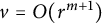 $v=O(r^{m+1}) $
. By Theorem 4.2 of [Reference Li and Tam16],
 $u\in C^{\infty }(B_1^m;B_{1}^n)\cap C^{m,\alpha }(\overline {B_1^m};\overline {B_{1}^n}), \forall \alpha \in (0,1)$
.
Let
 $$\begin{align*}\overline{w}_{m+1}=\overline{w}+\overline{\phi}_{m+1}d^{m+1}. \end{align*}$$
By (4.25), for any
 $s\geq 0$
, we have
 $$\begin{align*}|\nabla^s_\theta(u-\overline{w}_{m+1})|=O(d^{m+2-\varepsilon}), \forall \varepsilon>0. \end{align*}$$
Furthermore, by Theorem 4.2 of [Reference Li and Tam16], for any non-negative integers j and s, it holds that
 $$\begin{align*}|\nabla^j\nabla^s_\theta(u-\overline{w}_{m+1})|=O(d^{m+2-j-\varepsilon}), \forall \varepsilon>0. \end{align*}$$
Let
 $\overline {w}_{m_0}=\phi _0+\sum \limits _{k=1}^{m_0}\overline {\phi }_k(x)d^k+\sum \limits _{k=m+1}^{m_0}\sum \limits _{l=1}^{[\frac {m_0-1}{m}]} \overline {\psi }_{k,l}(x)d^k(\log (-d))^l$
. We assume, by induction, that the following inequality has been established for
 $m=m_0\geq m+1$
and for all non-negative integers j and s,
 $$ \begin{align} \begin{aligned} |\nabla^j\nabla^s_\theta(u-\overline{w}_{m_0})|=O(d^{m_0+1-j-\varepsilon}). \end{aligned} \end{align} $$
In Theorem 2.8, solving the equation
 $\overline {B}_{m_0+1}[u]+\overline {F}_{m_0+1}[u]+\overline {E}_{m_0+1}[u]=0$
is equivalent to finding
 $\overline {\phi }_{m_0+1}$
that satisfies this relationship. Similarly, the set of equations
 $\overline {B}_{m_0+1,l}[u]+\overline {F}_{m_0+1,l}[u]+\overline {E}_{m_0+1,l}[u]=0$
for
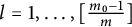 $l=1,\ldots ,[\frac {m_0-1}{m}]$
is used to determine the coefficients
 $\overline {\psi }_{m_0+1,l}$
. We then define the function
 $$\begin{align*}\overline{w}_{m_0+1}:=\phi_0+\sum\limits_{k=1}^{m_0+1}\overline{\phi}_k(x)d^k+\sum\limits_{k=m+1}^{m_0}\sum\limits_{l=1}^{[\frac{m_0-1}{m}]} \overline{\psi}_{k,l}(x)d^k(\log (-d))^l.\end{align*}$$
We have
 $$ \begin{align} \begin{aligned} \tau(\overline{w}_{m_0+1})=O(d^{m_0+2}\log(-d)). \end{aligned} \end{align} $$
Based on equation (4.27), we can establish an estimate for the difference between u and
 $\overline {w}_{m_0+1}$
. For any non-negative integers j and s, we have
 $$ \begin{align} \begin{aligned} &|\nabla^j\nabla^s_\theta(u-\overline{w}_{m_0+1})|\\& \quad =|\nabla^j\nabla^s_\theta(u-\overline{w}_{m_0}-\overline{\phi}_{m_0+1}d^{m_0+1}-\sum\limits_{l=1}^{[\frac{m_0}{m}]} \overline{\psi}_{m_0+1,l}(x)d^{m_0+1}(\log (-d))^l)|\\& \quad =O(d^{m_0+1-j-\varepsilon}). \end{aligned} \end{align} $$
Set
 $v_{m_0+1}:=u-\overline {w}_{m_0+1}$
and
 $v^0_{m_0+1}:=\langle u-\overline {w}_{m_0+1},\phi _0\rangle $
. Similar to the process used to derive equation (4.10), and by leveraging the result in (4.28), we can obtain
 $$ \begin{align} \begin{aligned} &Lv_{m_0+1}-(m-2)\langle v_{m_0+1} , \phi_0\rangle\phi_0\\& \quad =O(d^{3})|\nabla^2_0 v_{m_0+1}|+O(d^{2-\varepsilon})|\nabla_0 v_{m_0+1}|\\& \qquad +O(d)(|v_{m_0+1}|+|\nabla_\theta v_{m_0+1}|)+O(d^{m_0+2}\log(-d)), \end{aligned} \end{align} $$
where linear operator L is defined in (4.6).
Multiplying both sides of equation (4.30) by the function
 $\phi _0$
, we get
 $$ \begin{align} \begin{aligned} &L\langle v_{m_0+1} , \phi_0\rangle-(m-2)\langle v_{m_0+1} , \phi_0\rangle\\& \quad =O(d^{3})|\nabla^2_0 v_{m_0+1}|+O(d^{2-\varepsilon})|\nabla_0 v_{m_0+1}|\\& \qquad +O(d)(|v_{m_0+1}|+|\nabla_\theta v_{m_0+1}|)+O(d^{m_0+2}\log(-d)). \end{aligned} \end{align} $$
Define
 $\varphi _{m_0+1}:=\nabla ^s_\theta (u-\overline {w}_{m_0+1})$
. Differentiating (4.31) with respect to
 $\theta $
, we know
 $\varphi ^0_{m_0+1}:=\nabla ^s_\theta \langle u-\overline {w}_{m_0+1}, \phi _0\rangle $
satisfies
 $$ \begin{align} \begin{aligned} &L\varphi^0_{m_0+1}-(m-2)\varphi^0_{m_0+1}\\& \quad =O(d^{3})|\nabla^2_0 \varphi_{m_0+1}|+O(d^{2-\varepsilon})|\nabla_0 \varphi_{m_0+1}|\\& \qquad +O(d)(|\varphi_{m_0+1}|+|\nabla_\theta \varphi_{m_0+1}|)+O(d^{m_0+2}\log(-d)). \end{aligned} \end{align} $$
As in the proof of Lemma 4.1, we know that
 $\varphi ^0_{m_0+1}=O((1-\rho )^{m_0+2-\varepsilon })$
. So we can conclude that
 $$ \begin{align} \begin{aligned} L\varphi_{m_0+1}=O((1-\rho)^{m_0+2-\varepsilon}). \end{aligned} \end{align} $$
Finally, by using equation (4.29), we can derive
 $$ \begin{align} \begin{aligned} \frac{(1-\rho^2)^2}{4}\frac{\partial ^2\varphi_{m_0+1}}{\partial \rho^2}+\sum\limits_{i=1}^m\frac{m(1-\rho^2)}{2}\rho\frac{\partial \varphi_{m_0+1}}{\partial \rho}=O(d^{m_0+2-\varepsilon}). \end{aligned} \end{align} $$
Define
 $r:=\frac {1-\rho }{1+\rho }$
, we can get
 $$ \begin{align} \begin{aligned} r^2\frac{\partial ^2\varphi_{m_0+1}}{\partial r^2}-mr\frac{\partial \varphi_{m_0+1}}{\partial r}=:\eta=O(r^{m_0+2-\varepsilon}). \end{aligned} \end{align} $$
Next, we introduce a new function
 $\xi _{m_0+1}(r):=\frac {\varphi _{m_0+1}(\theta _0,r)}{r^{m+1}}$
. By substituting
 $\varphi _{m_0+1}=r^{m+1}\xi _{m_0+1}(r)$
into the previous equation, we obtain
 $$ \begin{align*} \begin{aligned} r^{m+3}\frac{\partial^2 \xi_{m_0+1}}{\partial r^2}+(m+2)r^{m+2}\frac{\partial \xi_{m_0+1}}{\partial r}&=r^2\frac{\partial^2 \varphi_{m_0+1}}{\partial r^2}-mr \frac{\partial \varphi_{m_0+1}}{\partial r}=O(r^{m_0+2-\varepsilon}),\\(r^{m+3}\xi_{m_0+1}^{'}(r))^{'} -r^{m+2}\xi_{m_0+1}^{'}(r)&=O(r^{m_0+2-\varepsilon}). \end{aligned} \end{align*} $$
Set
 $y_{m_0+1}=r^{m+3}\xi _{m_0+1}^{'}(r)$
, then
 $$ \begin{align*} \begin{aligned} ry_{m_0+1}^{'}(r)-y_{m_0+1}=:\pi_{m_0+1}=O(r^{m_0+3-\varepsilon}) \end{aligned} \end{align*} $$
has solution
 $$ \begin{align*} \begin{aligned} y_{m_0+1}(r)=r(\int_0^r R^{-2}\pi(R)\mathrm{d} R+\widetilde{C}). \end{aligned} \end{align*} $$
Therefore,
 $y_{m_0+1}=O(r^{m_0+3-\varepsilon })$
and
 $\xi _{m_0+1}=O(r^{m_0-m+1-\varepsilon })$
, which gives
 $\varphi _{m_0+1}=O(r^{m_0+2-\varepsilon })$
.
We may then argue as Theorem 4.2 of [Reference Li and Tam16] to obtain the regularity of u. For any non-negative integers j and s,
 $|\nabla ^s_\theta \nabla ^j_\rho (u-\overline {w}_{m_0+1})|=O(d^{m_0+2-j-\varepsilon }), \forall \varepsilon \in (0,1)$
.
Acknowledgements
Special thanks are extended to Professor Jingang Xiong for suggesting this research problem and for his continuous guidance throughout the study.



