1. Introduction
Toroidal drops present a phenomenon in fluid dynamics which has attracted the attention of researchers since they were observed in the experiments by Plateau (Reference Plateau1857) in rotating fluid. In recent years, the interest in this non-trivial form of fluid particles has been stimulated by new applications of non-spherical microparticles which have important potential as building blocks for self-assembled materials, imaging probes for therapy or drug carriers (see, e.g., Velev, Lenhoff & Kaler (Reference Velev, Lenhoff and Kaler2000), a review by Champion, Katare & Mitragotri (Reference Champion, Katare and Mitragotri2007) and more recent papers by Pairam et al. (Reference Pairam, Vallamkond, Koning, Benjamin, van Zuiden, Ellis, Bates, Vitelli and Fernández-Nieves2013) and Senyuk et al. (Reference Senyuk, Liu, He, Kamien, Kusner, Lubensky, Ivan and Smalyukh2013)). One advanced method of producing microparticles of complex shape is solidification of drops deformed by the flow in which they are embedded in microfluidic devices, see, e.g., Dendukuri et al. (Reference Dendukuri, Tsoi, Hatton and Doyl2005), Wang, Shum & Weitz (Reference Wang, Shum and Weitz2009) and Shum et al. (Reference Shum, Abate, Lee, Studart, Wang, Chen, Thiele, Shah, Krummel and Weitz2010). Thus, it is important to investigate the shape of drops in various types of flow. This work addresses the behaviour of drops of toroidal shape in a viscous flow.
Toroidal drops can be obtained in number of ways, including but not limited to the following.
-
(1) In rotating fluid, as in the experiments by Plateau (Reference Plateau1857), relying on inertial forces, and as in recent studies by Pairam & Fernández-Nieves (Reference Pairam and Fernández-Nieves2009), relying on viscous stresses.
-
(2) In the course of free fall of a large drop in an immiscible fluid (Baumann et al. Reference Baumann, Joseph, Mohr and Renardy1992; Sostarecz & Belmonte Reference Sostarecz and Belmonte2003).
-
(3) By the impact of a droplet with a superhydrophobic surface (Renardy et al. Reference Renardy, Popinet, Duchemin, Renardy, Zaleski, Josserand, Drumright-Clarke, Richard, Clanet and Quéré2003).
-
(4) By deformation of a drop in an electric (Deshmukh & Thaokar Reference Deshmukh and Thaokar2013; Ghazian, Adamiak & Castle Reference Ghazian, Adamiak and Castle2013) or magnetic field (Texier et al. Reference Texier, Piroird, Quéré and Clanet2013).
Of particular interest, with significance in geophysical flows, are swarms of particles that can evolve in a viscous fluid into toroidal shape (Machu et al. Reference Machu, Meile, Nitsche and Schaflinger2001b ; Bosse et al. Reference Bosse, Kleiser, Härtel and Meiburg2005). They resemble ‘drops’ of similar viscosity but have practically zero surface tension and behave dynamically as if composed of an immiscible different phase. The exciting field of drop deformation in electric and magnetic fields is beyond the scope of this paper. Below, we present a brief review of studies of viscous toroidal drops in the absence of such forces.
Pairam & Fernández-Nieves (Reference Pairam and Fernández-Nieves2009) reported experiments on the formation of fluid tori in rotating viscous fluid. It was demonstrated that once formed, the torus transforms into single or multiple spheres. The dynamics scenario depends on the aspect ratio of the torus: for extended thin tori, classical hydrodynamic instabilities develop and the torus breaks up into several droplets, while sufficiently fat tori shrink towards their centre and coalesce onto themself, forming a single spherical droplet. The experiments by Pairam & Fernández-Nieves (Reference Pairam and Fernández-Nieves2009) have inspired a number of theoretical studies of these two modes of toroidal drop dynamics. Thus, approximate models assuming a circular cross-section of the torus were suggested to describe the dynamics of the capillary-induced shrinking of toroidal drops. Yao & Bowick (Reference Yao and Bowick2011) studied the dynamics of a toroidal drop embedded into a viscous flow that was at rest far from the drop. Energy considerations were used to derive an equation reminiscent of the Rayleigh–Plesset equation for the collapse of transient cavities. Some physical considerations were presented to justify the circular shape assumption and the aspect ratio of the torus beyond which the Rayleigh instability overcomes the shrinking mode. Texier et al. (Reference Texier, Piroird, Quéré and Clanet2013) employed a potential flow approach to describe the dynamics of a fluid torus and obtained another variant of the Rayleigh–Plesset equation for the dynamics of toroidal drop collapse. Mehrabian & Feng (Reference Mehrabian and Feng2013) simulated a three-dimensional (3D) dynamics of a Newtonian torus suspended in a surrounding Newtonian liquid using finite elements on an unstructured and adaptively generated grid. Initially, sinusoidal disturbances were introduced on the torus and the effect of the retraction and the axial curvature on the growth rate of these disturbances was studied. The nonlinear instability and the final breakup into droplets were simulated as well. The numerical results were compared with the experiment of Pairam & Fernández-Nieves (Reference Pairam and Fernández-Nieves2009). The three theoretical works cited above consider the flow induced solely by surface tension in the absence of external forcing. Under such conditions solely spherical stationary drops are possible, and the studies were focused on the dynamic behaviour of the collapsing and breaking toroidal drops.
A number of works address stationary fluid tori with free surfaces in solid-body rotation, reflecting the original Plateau experiments. The shape of such a fluid body is determined by the interplay of centrifugal force and surface tension. Gulliver (Reference Gulliver1984) rigorously proved the existence of toroidal solutions of the governing equilibrium equations. Hynd & MacCuan (Reference Hynd and MacCuan2006) reported on further study of the existence and uniqueness of free rotating tori. Slobozhanin (Reference Slobozhanin1968) proved that all rotationally symmetric fluid tori are unstable to non-axisymmetric disturbances. Heine (Reference Heine2006) reported on the numerical computation of equilibrium rotating drops, including beautiful non-axisymmetric toroidal shapes. Zhao & Tao (Reference Zhao and Tao2013) analysed the base state and the surface-tension-induced instabilities of an inviscid liquid rotating ring considering the effects of the radius ratio, the normal velocity and the tangential velocity. Fontelos, Garcia-Garrido & Kindelian (Reference Fontelos, Garcia-Garrido and Kindelian2011) studied the evolution of rotating viscous drops embedded into viscous fluid rotating with the same angular velocity. The Stokes regime was assumed and the boundary integral formulation was employed. Various regimes of axisymmetric and 3D evolution were found, including stationary and evolving toroidal drops. Recently, Nurse, Coriell & McFadden (Reference Nurse, Coriell and McFadden2015) reported computed solutions for the axisymmetric equilibrium of toroidal (and spheroidal) drops or bubbles and a stability study of these shapes via computations of the second variation of the energy functional.
Kojima, Hinch & Acrivos (Reference Kojima, Hinch and Acrivos1984) reported the existence of toroidal shapes for drops in a viscous domain as a result of deformation of drops settling in a quiescent fluid, as a consequence of an interfacial instability induced by a finite surface perturbation. They also studied the dynamics of a highly expanded slender toroidal drop, making use of matched asymptotic expansion techniques, and showed that such a settling drop can expand only if small effects of inertia are incorporated into the analysis. On the other hand, the more recent numerical simulations by Machu et al. (Reference Machu, Meile, Nitsche and Schaflinger2001a ) demonstrated that the non-slender torus can also expand in quasi-static Stokes flow. As was mentioned above, such toroidal drops are constantly expanding and never achieve stationary configurations. The velocity field inside such a drop is characterized by the presence of a single vortex. No theoretical studies on toroidal drops in non-trivial viscous flow, other than in quiescent or rotating fluid, are available in the literature so far. The subject of this work is to study the deformation of fluid tori embedded in an axisymmetric compressional viscous flow (also known as biaxial extension).
In a recent study on the deformation of simply connected viscous drops in an axisymmetric compressional viscous flow, Zabarankin et al. (Reference Zabarankin, Smagin, Lavrenteva and Nir2013) showed that the drops deform to steady oblate shapes, characterized by a small half-thickness to radial extension ratio (aspect ratio) until critical conditions for the intensity of the flow condition are obtained. The latter is characterized by the capillary number (the ratio of viscous to capillary forces). For near-critical conditions, the shape of the drop is almost flat in the centre regions. However, the aspect ratios of such steady deformations were limited, and steady stationary shapes could not be obtained when the intensity of the flow increased any further. Remarkably, the critical aspect ratio appeared to be insensitive to the viscosity ratio of the immiscible fluids, and was very similar in cases with two fluids of equal viscosity and in cases involving embedded high-viscosity drops or inviscid bubbles. In cases of drop to ambient viscosity ratios of order unity or higher, Zabarankin et al. (Reference Zabarankin, Smagin, Lavrenteva and Nir2013) found that dimples of negative curvature appeared at the axis of symmetry. Dynamic simulations by Stone & Leal (Reference Stone and Leal1989) demonstrated that at supercritical capillary number, a fast thinning occurs near the middle of the drop, forming a nearly flat layer enclosed by a large bulbous ring. The authors argued that this shape continues to stretch and thin until the width of the layer becomes so small that intermolecular forces will lead to its breakup and the formation of a liquid torus. Such tori, embedded in the viscous compressional flow, are studied here.
The contribution and organization of this work are as follows. The problem of dynamic and stationary deformation of a drop in linear compressional viscous flow is formulated in § 2. Section 3 outlines dynamic simulations of axisymmetric toroidal drops and presents their results, which suggest, in particular, the existence of unstable stationary shapes at small enough capillary number. The asymptotic case of capillary-dominated flow (torus dynamics in a quiescent viscous fluid) is considered separately. The results of simulation in this case are compared with the experiments of Pairam & Fernández-Nieves (Reference Pairam and Fernández-Nieves2009). Section 4 presents a variational formulation of the problem of stationary toroidal drops in compressional flow and finds approximate solutions to this problem in the form of tori with circular and elliptic cross-sections. The findings of this work are summarized and discussed in § 5. Appendix A includes auxiliary results.
2. Problem formulation
Consider a drop of volume
 $4{\rm\pi}\,l^{3}/3$
(equal to that of a sphere with radius
 $l$
) and viscosity
 ${\it\mu}^{+}$
that is embedded in an unbounded compressional viscous flow with viscosity
 ${\it\mu}^{-}$
. The ratio
 ${\it\mu}^{+}/{\it\mu}^{-}$
will be denoted by
 ${\it\lambda}$
. Let
 $(x_{1},x_{2},x_{3})$
be a Cartesian coordinate system with the basis
 $(\boldsymbol{e}_{1},\boldsymbol{e}_{2},\boldsymbol{e}_{3})$
. In the absence of the drop, the ambient fluid is subject to an undisturbed flow:
 $$\begin{eqnarray}\boldsymbol{u}^{\infty }=G\left(x_{1}\,\boldsymbol{e}_{1}+x_{2}\,\boldsymbol{e}_{2}-2x_{3}\,\boldsymbol{e}_{3}\right),\end{eqnarray}$$
where
 $G$
is a constant shear rate, characterizing the intensity of the flow.
Let
 $V^{+}$
and
 $V^{-}$
denote the closed domain occupied by the drop with the interface
 $S$
, and the open domain occupied by the ambient fluid respectively. Let
 $\boldsymbol{u}^{+}=u_{k}^{+}\boldsymbol{e}_{k}$
and
 $\boldsymbol{u}^{-}=u_{k}^{-}\boldsymbol{e}_{k}$
be the actual velocity in
 $V^{+}$
and the disturbance velocity in
 $V^{-}$
respectively, and let
 $p^{\pm }$
be the pressure in
 $V^{\pm }$
. It should be noted that the actual velocity in
 $V^{-}$
is
 $\boldsymbol{u}^{\infty }+\boldsymbol{u}^{-}$
. Further on, we assume a creeping flow, i.e. the fields
 $\boldsymbol{u}^{\pm }$
and
 $p^{\pm }$
satisfying the stationary Stokes equations
 $$\begin{eqnarray}{\it\mu}^{\pm }\,u_{i,\,jj}^{\pm }=p_{,i},\quad u_{j,\,j}^{\pm }=0\quad \text{in }V^{\pm },\end{eqnarray}$$
with the following boundary conditions at
 $S$
and at infinity:
 $$\begin{eqnarray}(u_{i}^{-}+u_{i}^{\infty }-u_{i}^{+})|_{S}=0,\quad u_{i}^{-}|_{\infty }=0,\quad p^{-}|_{\infty }=0.\end{eqnarray}$$
In the case of the drop and ambient fluid having equal viscosities, i.e. when
 ${\it\lambda}=1$
, a stress balance across the interface results in simplified stress boundary conditions:
 $$\begin{eqnarray}p^{+}-p^{-}={\it\gamma}\,\text{div}_{S}\,\boldsymbol{n},\quad (u_{i,j}^{+}-u_{j,i}^{+})n_{j}=(u_{i,j}^{-}-u_{j,i}^{-})n_{j}\quad \text{on }S,\end{eqnarray}$$
where
 $\boldsymbol{n}=n_{k}\,\boldsymbol{e}_{k}$
is the outward normal to the surface
 $S$
,
 $\text{div}_{S}$
is the surface divergence operator (see, e.g., Aris Reference Aris1962) and
 ${\it\gamma}$
is the interfacial tension.
At the moving interface between the two immiscible fluids, the normal velocity
 $u_{n}^{+}$
equals the velocity
 ${\mathcal{U}}_{n}$
of the interface
 $S$
in the direction of
 $\boldsymbol{n}$
:
 $$\begin{eqnarray}u_{n}^{+}\equiv u_{i}^{+}n_{i}={\mathcal{U}}_{n}.\end{eqnarray}$$
In what follows, the length and the velocity and pressure fields are scaled with
 $l$
,
 $Gl$
and
 ${\it\mu}^{-}G$
respectively, and the capillary number is introduced as
 $Ca={\it\mu}^{-}Gl/{\it\gamma}$
. For the sake of simplicity, we keep the same notations for the scaled variables.
When
 ${\it\lambda}=1$
, the problem (2.2)–(2.4) is governed by a single parameter
 $Ca$
. For arbitrary
 $S$
, it admits a closed-form solution (see, e.g., Rallison & Acrivos Reference Rallison and Acrivos1978; Pozrikidis Reference Pozrikidis1992),
 $$\begin{eqnarray}\displaystyle & \displaystyle u_{i}^{\pm }(\boldsymbol{x})=\frac{1\pm 1}{2}u_{i}^{\infty }(\boldsymbol{x})-\frac{1}{Ca}\oint _{S}J_{ij}(\,\boldsymbol{y}-\boldsymbol{x})n_{j}(\,\boldsymbol{y})\text{div}_{S}\,\boldsymbol{n}(\,\boldsymbol{y})\,\text{d}S_{y},\quad \boldsymbol{x}\in V^{\pm }, & \displaystyle\end{eqnarray}$$
 $$\begin{eqnarray}\displaystyle & \displaystyle p^{\pm }(\boldsymbol{x})=\pm \frac{\text{div}_{S}\,\boldsymbol{n}(\boldsymbol{x})}{2Ca}{\mathcal{I}}_{\{\boldsymbol{x}\in S\}}+\frac{1}{4{\rm\pi}\,Ca}\oint _{S}\frac{n_{i}(\,\boldsymbol{y})(y_{i}-x_{i})}{\Vert \boldsymbol{y}-\boldsymbol{x}\Vert ^{3}}\text{div}_{S}\,\boldsymbol{n}(\,\boldsymbol{y})\,\text{d}S_{y},\quad \boldsymbol{x}\in V^{\pm }, & \displaystyle\end{eqnarray}$$
where
 $\boldsymbol{x}=x_{k}\,\boldsymbol{e}_{k}$
,
 $\boldsymbol{y}=y_{k}\,\boldsymbol{e}_{k}$
,
 $J_{ij}(\boldsymbol{x})$
is the fundamental solution of the Stokes equations (2.2), or so-called Stokeslet,
 $$\begin{eqnarray}J_{ij}(\boldsymbol{x})=\frac{1}{8{\rm\pi}}\left(\frac{{\it\delta}_{ij}}{\Vert \boldsymbol{x}\Vert }+\frac{x_{i}x_{j}}{\Vert \boldsymbol{x}\Vert ^{3}}\right),\quad {\it\delta}_{ij}=\left\{\begin{array}{@{}cc@{}}1, & i=j,\\ 0, & i\neq j,\end{array}\right.\end{eqnarray}$$
and
 ${\mathcal{I}}_{\{\boldsymbol{x}\in S\}}$
is the indicator function equal to 1 if
 $\boldsymbol{x}\in S$
and equal to 0 if
 $\boldsymbol{x}\not \in S$
. The representation (2.7) follows from the fact that
 $p=p^{\pm }$
is a harmonic function in
 $V^{\pm }$
having jump
 $Ca^{-1}\,\text{div}_{S}\,\boldsymbol{n}$
across
 $S$
. It is essentially a double-layer potential and holds for those
 $\boldsymbol{x}\in S$
at which
 $S$
is smooth.
At a stationary state, the shape of the drop does not change with time, i.e.
 $$\begin{eqnarray}{\mathcal{U}}_{n}(\boldsymbol{x})=u_{n}^{+}(\boldsymbol{x})=0,\quad \boldsymbol{x}\in S.\end{eqnarray}$$
With the representation (2.6), the condition (2.9) yields a nonlinear equation for finding a stationary-state shape
 $S$
:
 $$\begin{eqnarray}u_{n}^{+}(\boldsymbol{x})\equiv \left(u_{i}^{\infty }(\boldsymbol{x})-\frac{1}{Ca}\oint _{S}J_{ij}(\,\boldsymbol{y}-\boldsymbol{x})n_{j}(\,\boldsymbol{y})\text{div}_{S}\,\boldsymbol{n}(\,\boldsymbol{y})\,\text{d}S_{y}\right)n_{i}(\boldsymbol{x})=0,\quad \boldsymbol{x}\in S.\end{eqnarray}$$
Equation (2.10) has a simply connected solution (oblate spheroidal-like shapes), obtained and studied in Zabarankin et al. (Reference Zabarankin, Smagin, Lavrenteva and Nir2013), and, as shown here, a doubly connected solution (toroidal shapes). One of the approaches to solve (2.10) numerically is to simulate quasi-stationary dynamic deformation of the drop starting from some initial shape (Rallison & Acrivos Reference Rallison and Acrivos1978), i.e. from a unit sphere or a torus with circular cross-section, as described in § 3. A corresponding procedure is described in detail in Zabarankin et al. (Reference Zabarankin, Smagin, Lavrenteva and Nir2013) and was efficient in finding stable stationary-state shapes for simply connected deformable drops in a compressional flow, see Zabarankin et al. (Reference Zabarankin, Smagin, Lavrenteva and Nir2013). However, it is not expected to converge to unstable stationary shapes. Alternatively, (2.10) can be reformulated as a calculus of variations problem – this approach is efficient in identifying approximate solutions (both stable and unstable) in a family of shapes with one or two free parameters (§ 4).
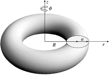
Toroidal drop:
 $R$
and
 $a$
are the major and minor radii respectively. The cross-section of the torus is shown in the
 $rz$
half-plane in the cylindrical coordinate system
 $(r,{\it\varphi},z)$
, where the
 $z$
-axis is the axis of revolution.

3. Numerical simulations
The drop dynamics simulations follow the general scheme for the quasi-stationary deformations.
-
(1) At time
 ${\it\tau}$
, start with some shape
$S_{{\it\tau}}$
.
-
(2) Divide
$S_{{\it\tau}}$
into
$N$
(evenly distributed) boundary elements and represent each element by a cubic spline parametrized by the arclength. -
(3) Express the normal unit vector
$\boldsymbol{n}$
and the curvature
$\text{div}\,\boldsymbol{n}$
of
$S_{{\it\tau}}$
in terms of the cubic spline coefficients explicitly. -
(4) Evaluate the boundary integral in (2.6) for
$\boldsymbol{x}\in S_{{\it\tau}}$
by the Gauss–Legendre quadrature with the so-called singularity subtraction (Pozrikidis Reference Pozrikidis1992) and output
$u_{n}^{+}$
. -
(5) If
$\Vert u_{n}^{+}\Vert <{\it\epsilon}$
for a given norm
$\Vert \cdot \Vert$
and accuracy
${\it\epsilon}$
, then stop, otherwise for a given time step
${\rm\Delta}{\it\tau}$
, advance
$S_{{\it\tau}}$
based on (2.5) as
$S_{{\it\tau}+{\rm\Delta}{\it\tau}}=S_{{\it\tau}}+u_{n}^{+}\,\boldsymbol{n}\,{\rm\Delta}{\it\tau}$
, set
${\it\tau}:={\it\tau}+{\rm\Delta}{\it\tau}$
and go to (2).




3.1. Dynamics
The initial shape of the drop is assumed to be a torus with circular cross-section and major radius
 $R$
, as depicted in figure 1. Since for the chosen scaled variables, the volume of the torus equals
 $4{\rm\pi}/3$
, the initial minor radius of the drop is
 $a=\sqrt{2/(3{\rm\pi}R)}$
. Here, we can take advantage of the axial symmetry of the drop and introduce a cylindrical coordinate system
 $(r,{\it\varphi},z)$
with the basis
 $(\boldsymbol{e}_{r},\boldsymbol{e}_{{\it\varphi}},\boldsymbol{e}_{z})$
, where the
 $z$
-axis coincides with the
 $x_{3}$
-axis. Equation (2.1) takes the form
 $\boldsymbol{u}^{\infty }=r\,\boldsymbol{e}_{r}-2z\,\boldsymbol{e}_{z}$
, and the problem (2.2)–(2.4) can be considered to be axisymmetric, i.e. independent of the angular coordinate
 ${\it\varphi}$
, so that
 $\boldsymbol{u}^{\pm }$
and
 $p^{\pm }$
are represented by
 $$\begin{eqnarray}\boldsymbol{u}^{\pm }=u_{r}^{\pm }(r,z)\,\boldsymbol{e}_{r}+u_{z}^{\pm }(r,z)\,\boldsymbol{e}_{z},\quad p^{\pm }=p^{\pm }(r,z).\end{eqnarray}$$
In this case, the integral representation (2.6) can be integrated over the angular coordinate
 ${\it\varphi}$
and simplified to expressions containing curvilinear integrals over the cross-section of the drop interface
 $S$
. The expressions for the hydrodynamic variables can be found in, e.g., (3.3) or (3.5a) and (3.5b) in Zabarankin et al. (Reference Zabarankin, Smagin, Lavrenteva and Nir2013) for the velocity and (3.9) and (3.10) in Zabarankin & Nir (Reference Zabarankin and Nir2011) for the pressure
 $p^{\pm }$
and vorticity
 $u_{i,j}^{\pm }-u_{j,i}^{\pm }$
; see also appendix A.
The drop dynamics is simulated for various values of
 $R$
and
 $Ca$
with
 $N=200$
and
 ${\rm\Delta}{\it\tau}=2\times 10^{-4}$
. The drop deformation is characterized by the major radius of the deformed torus, by the Taylor deformation factor of the torus and by a deformation factor of the torus cross-section,
 $$\begin{eqnarray}\displaystyle R({\it\tau})=\frac{R_{max}+R_{min}}{2},\quad D_{\mathit{torus}}=\frac{R_{max}-z_{max}}{R_{max}+z_{max}},\quad D_{\mathit{cross}\text{-}\mathit{section}}=\frac{R_{max}-R_{min}-2z_{max}}{R_{max}-R_{min}+2z_{max}} & & \displaystyle \nonumber\\ \displaystyle & & \displaystyle\end{eqnarray}$$
respectively, where
 $R_{max}$
and
 $R_{min}$
denote maximum and minimum distances of the drop interface from the
 $z$
-axis and
 $$\begin{eqnarray}z_{max}=\displaystyle \max _{(r,{\it\varphi},z)\in S}z.\end{eqnarray}$$
It should be recalled that the Taylor deformation factor varies between 0 and 1. The limiting behaviour
 $D_{\mathit{torus}}\rightarrow 1$
corresponds to
 $R_{max}\gg z_{max}$
, i.e. to a highly expanded thin torus. The opposite limit
 $D_{\mathit{torus}}=0$
would mean that
 $R_{max}=z_{max}$
. The latter equality is impossible for circular tori. Thus, the initial value of this parameter in our computations is always positive,
 $$\begin{eqnarray}D_{\mathit{torus}}(0)=\frac{R}{R+2a}>\frac{1}{3}\text{ (corresponds to the closed torus)}.\end{eqnarray}$$
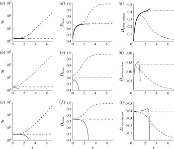
Time evolution of parameters of deforming initially circular tori. (a–c) Major radius of the toroid. (d–f) Taylor deformation factor of the torus. (g–i) Deformation factor of the torus cross-section. In (a,d,g),
 $Ca=0.18$
; dashed curves,
 $R=0.82$
; solid curves,
 $R=0.81$
; dot-dashed curves,
 $R=0.8107$
. In (b,e,h),
 $Ca=0.1$
; dashed curves,
 $R=1.2$
; solid curves,
 $R=1$
; dot-dashed curves,
 $R=1.09327$
. In (c,f,i),
 $Ca=0.04$
; dashed curves,
 $R=1.9$
; solid curves,
 $R=1.86$
; dot-dashed curves,
 $R=1.86969$
.

Dynamic deformation of the cross-section of an initially circular toroidal drop:
 $Ca=0.16$
; (a)
 $R=0.86$
; (b)
 $R=0.85236$
; (c)
 $R=0.852$
.

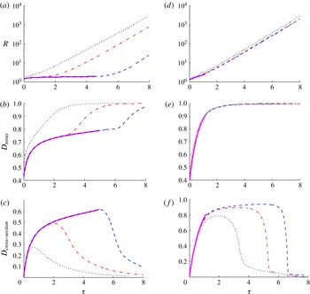
Figure 2 shows the typical evolution of these parameters at relatively small values of
 $Ca$
. In all of these cases,
 $R({\it\tau})$
and
 $D_{\mathit{torus}}$
initially increase. If the initial major radius
 $R$
exceeds some critical value
 $R_{cr}$
, the torus expands indefinitely,
 $R({\it\tau})$
and
 $D_{\mathit{torus}}$
grow monotonically with time. In these cases, shown by the dashed curves,
 $D_{\mathit{torus}}\rightarrow 1$
and
 $R({\it\tau})$
exhibits exponential growth as
 ${\it\tau}\rightarrow \infty$
. If
 $R<R_{cr}$
, then after initial growth,
 $R({\it\tau})$
and
 $D_{\mathit{torus}}$
attain maximum values and then decrease (see the solid curves). Finally, for
 $R\sim R_{cr}$
, after initial increase, all of the parameters approach some ‘equilibrium’ value and remain visibly constant for a relatively long time (dot-dashed curves). The initial period of deformation grows rapidly with increase of
 $Ca$
. Remarkably, the dependence of the equilibrium value of
 $D_{\mathit{torus}}$
on
 $Ca$
is not monotonic: the ‘equilibrium’ shapes for both
 $Ca=0.04$
and
 $Ca=0.18$
are more deformed than that for
 $Ca=0.1$
; see figure 2(d–f).
It is evident from figure 2(g–i) that, in all these cases, the cross-section initially elongates in the
 $r$
direction and
 $D_{\mathit{cross}\text{-}\mathit{section}}$
increases. Since initially the torus has a circular cross-section,
 $D_{\mathit{cross}\text{-}\mathit{section}}(0)=0$
. The initial period of elongation grows rapidly with increase of
 $Ca$
. Then,
 $D_{\mathit{cross}\text{-}\mathit{section}}$
either approaches some ‘equilibrium’ value, which remains visibly constant for a long time (dot-dashed curves), or attains a maximum and then decreases (solid curves). The ‘equilibrium’ deformation of the cross-section increases monotonically with
 $Ca$
. In the case of expansion (dashed curves),
 $D_{\mathit{cross}\text{-}\mathit{section}}\rightarrow 0$
as
 ${\it\tau}\rightarrow \infty$
, i.e. the shape of the drop becomes close to an expanding circular torus, and the maximum deformation is smaller than the ‘equilibrium’ one. In the case of contraction (solid curves),
 $D_{\mathit{cross}\text{-}\mathit{section}}$
attains a maximum, which is greater than the equilibrium value, and then decreases as the torus collapses towards the
 $z$
-axis (see figure 3
c).
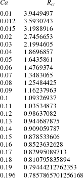
Critical major radius,
 $R_{cr}$
, for various values of
 $Ca$
.

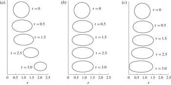
Dynamic deformation of the cross-section of an initially circular toroidal drop: (a)
 $Ca=0.04$
,
 $R=1.2$
; (b)
 $Ca=0.1$
,
 $R=1$
; (c)
 $Ca=0.15$
,
 $R=0.86$
.

Deformation parameters of the torus in two cases: (a–c)
 $Ca=0.2$
and (d–f)
 $Ca=0.5$
. In (a–c), the dotted, dot-dashed, dashed and solid curves correspond to
 $R=1$
, 0.786, 0.780438260324 and 0.780438260323 respectively, whereas in (d–f), they correspond to
 $R=0.8$
, 0.7, 0.6846 and 0.6845 respectively.

While figure 2 summarizes three types of drop dynamic deformation behaviour observed for
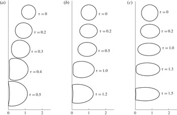
 $Ca\lesssim 0.19$
, figure 3 exemplifies these types of behaviour and change of cross-section shapes for
 $Ca=0.16$
and for
 $R$
assuming supercritical, near-critical and subcritical values.
In summary, the circular cross-section of the torus initially elongates in the
 $r$
direction. Then, the torus either contracts to the
 $z$
-axis or expands indefinitely. For any
 $Ca$
below a critical capillary number
 $Ca_{cr}$
, there exists a critical major radius
 $R_{cr}$
of the initial circular torus, separating these two scenarios (see figure 3
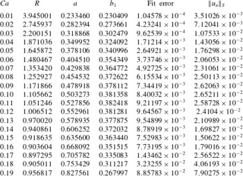
a,c) and estimated from table 1 as a function of
 $Ca$
to be
 $$\begin{eqnarray}\displaystyle R_{cr}(Ca)\approx 0.588678\cdot Ca^{-0.44371}+2.37196\cdot Ca^{1.61282}-0.598646,\quad Ca\in [0.01,0.196],\hspace{-10.00002pt} & & \displaystyle \nonumber\\ \displaystyle & & \displaystyle\end{eqnarray}$$
with a mean absolute error of
 $8.4\times 10^{-4}$
. For
 $Ca<Ca_{cr}$
and
 $R\sim R_{cr}$
, after initial elongation, the drop maintains the same shape for a relatively long time (figure 3
b), which suggests the existence of unstable stationary shapes of viscous toroids – the subject of § 4. One can expect that this time can be made as long as desired with a very accurate choice of
 $R$
. However, in practical calculations, we are restricted by the computer accuracy (the number of digits). Here, we assume ‘relatively long time’ to be
 ${\it\tau}^{\ast }\sim 6$
. The values of
 $R_{cr}$
that are presented in table 1 satisfy the above definition for
 $Ca\leqslant 0.19$
. For
 $Ca=0.196$
, the maximal time of stay at ‘equilibrium’ achievable with 15 digits of
 $R$
equals 3. Table 1 shows that the needed accuracy of
 $R_{cr}$
increases with
 $Ca$
– the greater
 $Ca$
is, the more accurately
 $R_{cr}$
should be determined to sustain a visually stationary cross-section for a prolonged period of time. Moreover, the lower
 $Ca$
is, the longer value of
 ${\it\tau}^{\ast }$
is available. (The above interpolating function of
 $R_{cr}(Ca)$
provides only a rough (and quick) estimate of
 $R_{cr}$
.)
Figure 3(c) shows that for
 $R<R_{cr}$
, the torus cross-section is deformed in the vicinity of the
 $z$
-axis when the interface approaches it. The inner part of the drop surface forms a thin almost circular cylinder centred at the
 $z$
-axis. It is anticipated that it will collapse, the drop will regain a simply connected shape and, with the passage of time, it will settle on the stationary shape studied in Zabarankin et al. (Reference Zabarankin, Smagin, Lavrenteva and Nir2013). However, the code stops when any point of the torus comes closer than
 $10^{-4}$
to the
 $z$
-axis (this is reflected by the fact that the solid curves in figure 2 do not span the full
 ${\it\tau}$
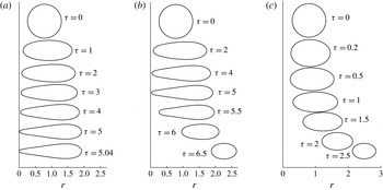
range), so that detailed investigation of the drop coalescence calls for a separate work. Figure 4(a–c) shows sequential stages of torus contraction for three pairs:
 $Ca=0.04$
,
 $R=1.2$
;
 $Ca=0.1$
,
 $R=1$
;
 $Ca=0.15$
,
 $R=0.86$
respectively. In all these cases, when the torus contracts to the
 $z$
-axis, the inner part of its cross-section straightens first and then develops a region of converted curvature at the centre. Thus, the closest approach of the interface to the
 $z$
-axis is not at the
 $z=0$
plane but rather at some distance from it. It should be noted that the concave and convex portions of the cross-section perimeter, depicted in figure 4, are connected by narrow regions of very high local curvature, although the interface is regular and continuous. With increase of
 $Ca$
, the torus cross-section becomes more elongated in the
 $r$
direction and the size of the straightened and dimpled region decreases. It is observed numerically that if
 $R<R_{cr}$
and
 $R\not \approx R_{0}=(3{\rm\pi}/2)^{-1/3}$
, where
 $R_{0}$
corresponds to a closed circular torus, the developed stage of contraction does not depend on
 $R$
.
Dynamic deformation of the initially circular cross-section of a toroidal drop for
 $Ca=0.2$
in three cases: (a)
 $R=0.780438260323$
, (b)
 $R=0.780438260324$
, (c)
 $R=0.8$
.

For
 $Ca>Ca_{cr}$
, no ‘equilibrium’ shapes that persist for a relatively long time were found, and the drop dynamics simulations suggest that
 $Ca_{cr}\in (0.19,0.2)$
. Figure 5 shows typical examples of the time evolution of
 $R({\it\tau})$
,
 $D_{\mathit{torus}}$
and
 $D_{\mathit{cross}\text{-}\mathit{section}}$
for
 $Ca>Ca_{cr}$
. In figures 5(a–c),
 $Ca=0.2$
and the dotted, dot-dashed, dashed and solid curves correspond to
 $R=1$
,
 $0.7806$
, 0.780438260324 and 0.780438260323 respectively. One can observe that, during the initial period, the cross-section elongates rapidly in the
 $r$
direction, the major radius and both deformation factors grow; then,
 $D_{\mathit{cross}\text{-}\mathit{section}}$
slows down and, if the initial
 $R>R_{cr}$
, it eventually begins to decrease. Moreover, after the initial rapid increase,
 $D_{\mathit{torus}}$
slows down but continues to grow, and then, after the cross-section begins to contract in the
 $r$
direction, it accelerates again. As time increases, the torus expands indefinitely, with the major radius increasing exponentially with time and with the cross-section approaching a circular shape. When
 $R<R_{cr}$
, the interface approaches the proximity of the
 $z$
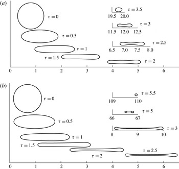
-axis and the code stops. These two types of behaviour are illustrated in figure 6(a,c), where cross-section shapes corresponding to figure 5(a–c) are shown at several time moments. In figure 6(a), where the process starts at
 $R=0.780438260323$
(solid curves in figure 5
a,b), the drop elongates in the
 $r$
direction, approaches the
 $z$
-axis, becomes thinner in the centre region and collapses. In figure 6(b), where
 $R=0.780438260324$
(dashed curves in figure 5
a,b) is greater than
 $R$
in figure 6(a) by just
 $10^{-12}$
, the drop behaves initially as in figure 6(a): it also approaches the
 $z$
-axis near the
 $z=0$
plane. However, its interface does not collapse, and the initial approach to the
 $z$
-axis is followed by contraction of the cross-section and expansion of the torus. In figure 6(c), where
 $R=0.8$
, no close approach to the
 $z$
-axis occurs, and the dynamic behaviour is similar to that described in the supercritical case for
 $Ca<0.19$
(see, e.g., figure 3
a). With the passage of time, the cross-section of the drop assumes an almost circular shape, and the torus expands indefinitely.
In figure 5(d–f), where
 $Ca=0.5$
, during the initial period the cross-section elongates rapidly in the
 $r$
direction and then slows down. If the initial
 $R\lesssim 0.6845$
, the torus collapses. For higher initial
 $R$
,
 $D_{\mathit{torus}}$
continues to grow rapidly, which contrasts the two stages evident in the case of
 $Ca=0.2$
. Figure 7 shows an evolving cross sections shape at this relatively high
 $Ca=0.5$
. In figure 7(a), where
 $R=0.8$
, considerable initial elongation occurs simultaneously with torus expansion. The cross-section first assumes an elliptic shape, then flattens, and forms a dimple. With the passage of time and as the torus expands further, the cross-section contracts and assumes an elliptic shape that becomes more and more circular. In figure 7(b), where
 $R=0.7$
, the deformation pattern is qualitatively similar to that observed for higher values of
 $R$
. However, in this case, the cross-section becomes more elongated and the dimple is more developed, so that the cross-section becomes very thin in its centre region and is even more susceptible to a potential breakup. Moreover, thin highly expanded tori may become unstable to disturbances, involving the azimuthal angle
 ${\it\varphi}$
, and break up in a non-axisymmetric manner. Nevertheless, if breaking does not occur, with further expansion of the torus, its cross-section contracts again and assumes an almost circular shape. Table 2 summarizes outcomes of deformation of circular tori with initial radius
 $R$
.
Dynamic deformation of the initially circular cross-section of a toroidal drop for
 $Ca=0.5$
in two cases: (a)
 $R=0.8$
and (b)
 $R=0.7$
.

3.2. Dynamics in the absence of external flow
The case of the absence of external flow corresponds to
 $Ca=0$
. The representation (2.6) is not directly applicable in this case. However, multiplying (2.6) by
 $Ca$
, rescaling the velocity and taking
 $Ca=0$
results in
 $$\begin{eqnarray}u_{i}^{\pm }(\boldsymbol{x})=-\oint _{S}J_{ij}(\,\boldsymbol{y}-\boldsymbol{x})n_{j}(\,\boldsymbol{y})\text{div}_{S}\,\boldsymbol{n}(\,\boldsymbol{y})\,\text{d}S_{y},\quad \boldsymbol{x}\in V^{\pm }.\end{eqnarray}$$
The rescaling implies that the velocity and time are scaled by
 $U^{\ast }={\it\gamma}/{\it\mu}^{-}$
and
 $t^{\ast }=l{\it\mu}^{-}/{\it\gamma}$
respectively. It should be noted that (3.6) contains no parameters.
Outcomes of deformation of circular tori with initial radius
 $R$
.

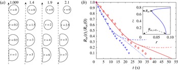
We employed (3.6) to simulate the dynamics of a torus in a quiescent fluid for initial conditions corresponding to those in Pairam & Fernández-Nieves (Reference Pairam and Fernández-Nieves2009) and Yao & Bowick (Reference Yao and Bowick2011). Figure 8(a) demonstrates typical dynamic deformations of initially circular fat tori with various initial aspect ratios,
 $R/a$
. Here, we chose the aspect ratio as a characteristic of the initial state (instead of
 $R$
which is used in the rest of the paper) in order to facilitate comparison with the available experimental data. This dynamics is qualitatively similar to that for a small capillary (see figure 4
a): the droplet first shrinks keeping an almost circular cross-section, then, as its inner part contracts to the
 $z$
-axis, considerable deformation takes place. The inner part of the drop surface forms a thin almost circular cylinder centred at the
 $z$
-axis and then develops a region of converted curvature in the centre. In contrast to the case of deformation in the presence of external compressional flow, no initial elongation in the
 $r$
direction occurs. It should be noted also that the developed stages of deformation are almost independent of the initial aspect ratio, unless the latter is very close to one (the case of a closed torus). In this case, no region of converted curvature is formed and the drop assumes an almost spherical shape with a thin cylindrical hole around the
 $z$
-axis.
(a) Dynamic deformation of the initially circular cross-section of a toroidal drop for
 $Ca=0$
in four cases:
 $R/a=1.009$
,
 $1.4$
,
 $1.9$
and
 $2.1$
. (b) The inner radius
 $R_{in}=\min _{\boldsymbol{x}\in S}r$
(dotted and solid curves) and
 $R_{in,\,z=0}=\min _{\boldsymbol{x}\in S,\,z=0}r$
(see inset) of the droplet normalized by its initial value for initial aspect ratios of 1.4 (dotted and dashed curves) and 1.9 (solid and dot-dashed curves). The physical parameters are taken from Pairam & Fernández-Nieves (Reference Pairam and Fernández-Nieves2009):
 ${\it\mu}=30\,000~\text{cp}$
,
 ${\it\sigma}=4~\text{mN}~\text{m}^{-1}$
.

In the experiments of Pairam & Fernández-Nieves (Reference Pairam and Fernández-Nieves2009), the drop to ambient fluid viscosity ratio was very small,
 ${\it\lambda}=1/30\,000$
, while in the theory developed in this paper
 ${\it\lambda}=1$
. A direct quantitative comparison between theory and experiments is, thus, not possible. However, assuming that the relevant time scale for drop deformation in viscous fluid is
 $l({\it\mu}^{+}+{\it\mu}^{-})/{\it\gamma}=(1+{\it\lambda})t^{\ast }$
, we concluded that the time scale for the experiment of Pairam & Fernández-Nieves (Reference Pairam and Fernández-Nieves2009) is approximately half of what it would be for
 ${\it\lambda}=1$
. In figure 8(b), the inner radius of the droplet normalized by its initial value is plotted versus
 $0.5t^{\ast }{\it\tau}$
for initial aspect ratios of 1.4 (dotted and dashed curves) and 1.9 (solid and dot-dashed curves). The physical parameters taken from Pairam & Fernández-Nieves (Reference Pairam and Fernández-Nieves2009) are
 ${\it\mu}=30\,000~\text{cp}$
,
 ${\it\sigma}=4~\text{mN}~\text{m}^{-1}$
and a volume of the drop of
 $272~\text{mm}^{3}$
. Two definitions of the inner radius are used:
 $R_{in}=\min _{\boldsymbol{x}\in S}r$
(dotted and solid curves) and
 $R_{in,\,z=0}=\min _{\boldsymbol{x}\in S,\,z=0}r$
(solid and dot-dashed curves), see the inset in figure 8(b). These two definitions coincide for circular tori, and, as it is evident in the figure, also during the initial period of torus deformation before the region of converted curvature is formed. Experimental data points taken from Pairam & Fernández-Nieves (Reference Pairam and Fernández-Nieves2009) are presented by triangle and diamond symbols. It is evident that, during the initial period, the curves in figure 8(b) are almost linear, and the agreement of the experimental data and computations is excellent. However, as the torus contracts, considerable deformations result in slowing down of the inner radius change, and the linearity of the curves is lost. At this stage, the computed results deviate from the experimental data. The predicted final contraction time is approximately 1.5 times as much as that observed experimentally. This difference can be attributed to the axial asymmetry of both the flow and the drop shape in the experiments reported by Pairam & Fernández-Nieves (Reference Pairam and Fernández-Nieves2009), which, evidently, enhances the self-coalescence of the torus.


3.3. Stationary shapes
In this subsection, the cross-sections of the slowly changing deformed shapes, resulting from dynamic simulations via (2.6) of initially circular tori with
 $R\simeq R_{cr}$
(see, e.g., figure 3
b) and referred to further as pointwise stationary shapes, are fitted by smooth curves parametrized by
 $$\begin{eqnarray}r(t)=R+a\cos t,\quad z(t)=\sin t\mathop{\sum }_{k=1}^{K}b_{k}\,T_{2(k-1)}(t/{\rm\pi}),\quad t\in [-{\rm\pi},{\rm\pi}],\end{eqnarray}$$
where
 $R$
,
 $a$
,
 $b_{1},\ldots ,b_{k}$
are parameters, and
 $T_{k}(t)$
is a
 $k\text{th}$
-order Chebyshev polynomial of the first kind. For
 $K=1$
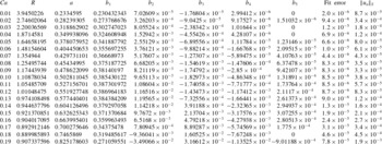
, (3.7) describes an ellipse. Tables 3 and 4 present parameters for (3.7) approximating the cross-sections of pointwise stationary-state shapes with
 $K=1$
and
 $K=5$
respectively. The tables also present the mean absolute value
 $\Vert u_{n}\Vert _{S}$
defined by
 $$\begin{eqnarray}\Vert u_{n}\Vert _{S}=\frac{\displaystyle \int _{\ell }|u_{n}^{+}|\,\text{d}s}{\displaystyle \int _{\ell }\,\text{d}s},\end{eqnarray}$$
where
 $u_{n}^{+}$
is determined by (2.10) and
 $\text{d}s=\sqrt{(r^{\prime }(t))^{2}+(z^{\prime }(t))^{2}}\,\text{d}t$
is the curve length element, and the fit error introduced by
 $$\begin{eqnarray}\sqrt{\frac{1}{N}\mathop{\sum }_{i=1}^{N}\left|\sqrt{1-\left(\frac{r_{i}-R}{a}\right)^{2}}\mathop{\sum }_{k=1}^{K}b_{k}\,T_{2(k-1)}\left(\frac{1}{{\rm\pi}}\arccos \frac{r_{i}-R}{a}\right)-z_{i}\right|^{2}},\end{eqnarray}$$
where
 $N=200$
is the number of points in the cross-section of a pointwise stationary-state shape.
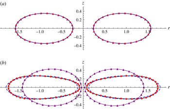
Cross-sections of the pointwise stationary-state shapes (solid curves) and their approximations by (3.7) with
 $K=1$
(fitted ellipses, dashed curves) and with
 $K=5$
(circles) in two cases: (a)
 $Ca=0.16$
and (b)
 $Ca=0.19$
. Triangles mark the cross-sections of corresponding ‘stationary’ elliptic tori found from the inverse problem (4.18) with
 $w=r^{-1}$
.

Figure 9(a,b) shows the cross-sections of the pointwise stationary-state shapes (solid curves) and their approximations by (3.7) with
 $K=1$
(fitted ellipses, dashed curves) and with
 $K=5$
(circles) in two cases: (a)
 $Ca=0.16$
and (b)
 $Ca=0.19$
. They also depict the cross-sections of the corresponding ‘stationary’ elliptic tori (triangles) found from the inverse problem (4.18) in § 4. In figure 9(a), all of the shapes are visually indistinguishable – elliptic tori are a remarkably good approximation for stationary-state shapes up to
 $Ca=0.16$
. In figure 9(b), the cross-section of the pointwise stationary-state shape is no longer elliptic – the deviation from the fitted ellipse is quite visible. In this case, the cross-section of the of ‘stationary’ elliptic torus differs considerably not only from that of the pointwise stationary shape, but also from the fitted ellipse, which yields a much smaller mean absolute value
 $\Vert u_{n}\Vert _{S}$
. (The reason why
 $\Vert u_{n}\Vert _{S}$
is smaller for the fitted elliptic torus is because the ‘stationary’ elliptic torus is found from the inverse problem rather than from direct minimization of
 $\Vert u_{n}\Vert _{S}$
; see § 4.1.) However, (3.7) with
 $K=5$
still provides an excellent approximation – the red circles firmly trace the solid curve.
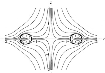
Streamlines about the stationary-state toroidal shape for
 $Ca=0.05$
.

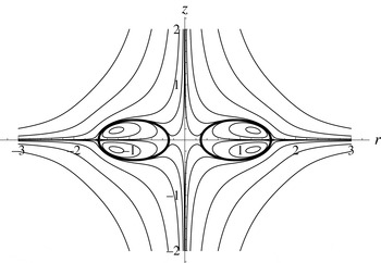
Streamlines about the stationary-state toroidal shape for
 $Ca=0.15$
.

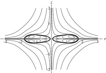
Streamlines about the stationary-state toroidal shape for
 $Ca=0.19$
.

Figures 10–12 show the streamline patterns inside and outside the cross-sections of the stationary-state drops in the
 $rz$
plane for
 $Ca=0.05$
, 0.15 and 0.19 respectively – the interface in all of these cases is a streamline, confirming that the drops are indeed at steady state. However, continuation of the dynamic computation for an extended time (this time grows with decrease of
 $Ca$
and with the accuracy of the initial radius
 $R$
) always results in destruction of these shapes, reflecting their possible instability. Thus, the search for stationary tori by dynamic computations is hindered by the need for extremely accurate initial conditions. In the next section we describe an alternative much more efficient method of finding these shapes.
4. Calculus of variations approach to finding stationary toroidal shapes
An alternative approach to finding stationary-state shapes is to cast (2.10) as a calculus of variations problem. For example, we can introduce error functionals by
 $$\begin{eqnarray}\mathscr{E}_{1}(u_{n}^{+},w;S)=\oint _{S}w(\boldsymbol{x})\left|u_{n}^{+}(\boldsymbol{x})\right|\text{d}S_{x},\quad \mathscr{E}_{2}(u_{n}^{+},w;S)=\sqrt{\oint _{S}w(\boldsymbol{x})\left[u_{n}^{+}(\boldsymbol{x})\right]^{2}\,\text{d}S_{x}},\end{eqnarray}$$
where
 $w$
is a positive weight function on
 $S$
, and minimize any of
 $\mathscr{E}_{1}$
and
 $\mathscr{E}_{2}$
in (4.1) with respect to
 $S$
subject to conditions that
 $u_{n}^{+}$
is given in (2.10) and that the volume of the drop is equal to
 $4{\rm\pi}/3$
:
 $$\begin{eqnarray}\min _{S}\mathscr{E}_{k}(u_{n}^{+},w;S)\quad \text{subject to the volume of the drop being equal to }4{\rm\pi}/3.\end{eqnarray}$$
Obviously, a shape
 $S$
satisfies (2.10) if and only if it yields zero minima for
 $\mathscr{E}_{1}$
or
 $\mathscr{E}_{2}$
. The problem (4.2) with (4.1) is a direct problem and is similar to the one in § 3.1 in Zabarankin (Reference Zabarankin2013). If the cross-section of
 $S$
in the
 $rz$
half-plane in the cylindrical coordinates is represented by a smooth curve with a finite number of parameters that satisfy the volume constraint identically, the problem (4.2) simplifies to finite parameter optimization. However, as a function of those parameters,
 $\mathscr{E}_{1}$
and
 $\mathscr{E}_{2}$
are unlikely to be convex, and, as a result, gradient-based methods (Ruszczyński Reference Ruszczyński2011) may converge slowly and be trapped in one of the local minima. In the case when the smooth curve has merely one or two free parameters, an approximation of a stationary shape can be efficiently found through an inverse problem formulated in the next section.
4.1. Inverse problem for finding approximate stationary shapes
Suppose that a family of shapes,
 $\mathscr{F}$
, is determined by a single free parameter, e.g. the major radius
 $R$
in circular tori of volume
 $4{\rm\pi}/3$
, and suppose that for a given
 $Ca$
, a ‘stationary’ shape minimizes
 $\mathscr{E}_{2}^{2}(u_{n}^{+},w;S)$
subject to
 $S\in \mathscr{F}$
. In this case, numerical optimization finds optimal
 $R$
iteratively, e.g. by the golden section method. (The complexity of the golden section method is the same as for the ordinary bisection method for finding a zero of a monotone function.) Then, in order to plot
 $R=R(Ca)$
, numerical optimization should be repeated for an array of values of
 $Ca$
, which is a computationally expensive procedure.
To find the curve
 $(Ca,R(Ca))$
approximately but with considerably less computational effort, Zabarankin (Reference Zabarankin2013) proposed to solve the inverse problem that interchanges the roles of
 $Ca$
and
 $R$
: for a given
 $R$
, minimize an error functional, e.g.
 $\mathscr{E}_{1}$
or
 $\mathscr{E}_{2}$
, with respect to
 $Ca$
. In this case,
 $\mathscr{E}_{2}^{2}(u_{n}^{+},w;S)$
is a quadratic function of
 $1/Ca$
,
 $$\begin{eqnarray}\mathscr{E}_{2}^{2}(u_{n}^{+},w;S)=\mathscr{E}_{2}^{2}(u_{n}^{\infty },w;S)-\frac{2}{Ca}\oint _{S}w(\boldsymbol{x})u_{n}^{\infty }(\boldsymbol{x})v(\boldsymbol{x})\,\text{d}S_{x}+\frac{1}{Ca^{2}}\mathscr{E}_{2}^{2}(v,w;S),\end{eqnarray}$$
where
 $$\begin{eqnarray}u_{n}^{\infty }(\boldsymbol{x})=u_{i}^{\infty }(\boldsymbol{x})n_{i}(\boldsymbol{x}),\quad v(\boldsymbol{x})=n_{i}(\boldsymbol{x})\oint _{S}J_{ij}(\,\boldsymbol{y}-\boldsymbol{x})n_{j}(\boldsymbol{y})\text{div}_{S}\,\boldsymbol{n}(\,\boldsymbol{y})\,\text{d}S_{y},\end{eqnarray}$$
so that an optimal
 $Ca$
can be determined analytically,
 $$\begin{eqnarray}Ca=\frac{\mathscr{E}_{2}^{2}(v,w;S)}{\displaystyle \oint _{S}w(\boldsymbol{x})u_{n}^{\infty }(\boldsymbol{x})v(\boldsymbol{x})\,\text{d}S_{x}},\end{eqnarray}$$
which yields
 $Ca=Ca(R)$
with no iteration procedure. In general, the curves
 $(Ca,R(Ca))$
and
 $(Ca(R),R)$
do not coincide. However, they do coincide when
 $\mathscr{E}_{2}(u_{n}^{+},w;S)=0$
and
 $R(Ca)$
and
 $Ca(R)$
are uniquely determined. When the corresponding optimal values of
 $\mathscr{E}_{2}(u_{n}^{+},w;S)$
are small, these curves are expected to be close.
For a family of shapes having two free parameters, one of the parameters can be assumed to be fixed,
 $Ca$
determined by (4.5) and the second parameter found by minimizing
 $\mathscr{E}_{2}^{2}(u_{n}^{+},w;S)$
with (4.5) by the golden section method. This approach is demonstrated in § 4.4.
4.2. ‘Stationary’ circular tori
In the
 $rz$
half-plane of the cylindrical coordinates
 $(r,{\it\varphi},z)$
, the cross-section of a circular torus having the volume of a unit sphere, i.e.
 $4{\rm\pi}/3$
, can be parametrized by
 $$\begin{eqnarray}r(t)=R+a\cos t,\quad z(t)=a\sin t,\quad a=\sqrt{\frac{2}{3{\rm\pi}R}},\quad t\in [-{\rm\pi},{\rm\pi}],\end{eqnarray}$$
where
 $R$
and
 $a$
are the major and minor torus radii respectively. In this case,
 $R\geqslant R_{0}=(3{\rm\pi}/2)^{-1/3}$
 ${\approx}0.596$
, where
 $R_{0}$
corresponds to a closed torus (with no opening), and
 $$\begin{eqnarray}\boldsymbol{n}(t,{\it\varphi})=\boldsymbol{e}_{r}\cos t+\boldsymbol{e}_{z}\sin t,\quad \text{div}_{S}\,\boldsymbol{n}(t,{\it\varphi})=\frac{1}{a}+\frac{\cos t}{R+a\cos t}.\end{eqnarray}$$
Section 3.1 shows that circular tori are never stationary: for
 $R<R_{cr}$
, a circular torus contracts to the
 $z$
-axis and regains a simply connected shape, whereas for
 $R>R_{cr}$
, it will expand indefinitely, where the critical radius
 $R_{cr}$
is found by the trial-and-error method (see table 1). Nonetheless, when
 $R=R_{cr}(Ca)$
and
 $Ca\rightarrow 0$
, the stationary toroid approaches a circular torus, and the circular torus analysis can provide accurate estimates of
 $R_{cr}$
. (A streamfunction satisfying the boundary conditions (2.3) and (2.4) for circular tori can be constructed in the toroidal coordinates
 $({\it\xi},{\it\eta})$
as in Zabarankin & Krokhmal (Reference Zabarankin and Krokhmal2007), where
 $({\it\xi},{\it\eta})$
are related to the cylindrical coordinates
 $(r,z)$
as
 $r=c\sinh {\it\xi}/(\cosh {\it\xi}-\cos {\it\eta})$
and
 $z=c\sin {\it\eta}/(\cosh {\it\xi}-\cos {\it\eta})$
, with
 ${\it\xi}\in [0,\infty )$
,
 ${\it\eta}\in [-{\rm\pi},{\rm\pi}]$
and
 $c$
being a positive metric parameter, see also Pell & Payne (Reference Pell and Payne1960) and Khuri & Wazwaz (Reference Khuri and Wazwaz1997).)
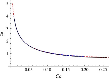
Circular tori:
 $(Ca,R(Ca))$
with
 $R(Ca)$
minimizing
 $\mathscr{E}_{1}(u_{n}^{+},r^{-1};S)$
(solid curve),
 $(Ca(R),R)$
with
 $Ca(R)$
determined by (4.9) (dot-dashed curve) and
 $(Ca,R_{cr}(Ca))$
with the critical radius
 $R_{cr}(Ca)$
tabulated in table 1 (dashed curve). The dashed and dot-dashed curves are visually indistinguishable.

Given that circular tori do not satisfy (2.10) identically, one of the approaches to find a ‘stationary’ torus is to minimize a kinematic condition error, e.g.
 $\mathscr{E}_{1}\left(u_{n}^{+},w;S\right)$
or
 $\mathscr{E}_{2}\left(u_{n}^{+},w;S\right)$
defined in (4.1), with respect to
 $R$
. Remarkably, the curve
 $(Ca,R(Ca))$
with
 $$\begin{eqnarray}R(Ca)=\mathop{\text{argmin}}_{R}\mathscr{E}_{1}\left(u_{n}^{+},r^{-1};S\right)\end{eqnarray}$$
is quite close to
 $(Ca(R),R)$
, with
 $$\begin{eqnarray}Ca(R)=\mathop{\text{argmin}}_{Ca}\mathscr{E}_{2}^{2}\left(u_{n}^{+},r^{-3};S\right)=\frac{\mathscr{E}_{2}^{2}\left(v,r^{-3};S\right)}{\displaystyle \oint _{S}r^{-3}(\boldsymbol{x})u_{n}^{\infty }(\boldsymbol{x})v(\boldsymbol{x})\,\text{d}S_{x}},\end{eqnarray}$$
and to the curve
 $(Ca,R_{cr}(Ca))$
, where
 $R_{cr}(Ca)$
is tabulated in table 1, see figure 13. In fact,
 $(Ca(R),R)$
with
 $Ca(R)$
determined by (4.9) is visually indistinguishable from
 $(Ca,R_{cr}(Ca))$
, and the inverse of
 $Ca(R)$
is estimated to be
 $$\begin{eqnarray}0.59335\cdot Ca^{-0.442585}+1.14997\cdot Ca^{1.17774}-0.61228,\quad Ca\in [0.00625,0.26],\end{eqnarray}$$
with a mean absolute error of
 $10^{-4}$
based on 26 tabulations.
In figure 14(b), triangles mark the curve
 $(Ca(R),a(R))$
, with
 $a(R)=\sqrt{2/(3{\rm\pi}R)}$
and
 $Ca(R)$
determined by (4.9).
4.3. Relationship between
$Ca$
and
$R$
for ‘stationary’ circular tori as
$Ca\rightarrow 0$


Section 4.2 suggests that
 $R(Ca)\rightarrow \infty$
as
 $Ca\rightarrow 0$
. In this case, the asymptotic behaviour of
 $Ca(R)$
as
 $R\rightarrow \infty$
can be obtained as follows. With (2.6) and (4.7),
 $u_{i}^{+}(\boldsymbol{x})$
takes the form
 $$\begin{eqnarray}u_{i}^{+}(\boldsymbol{x})=u_{i}^{\infty }(\boldsymbol{x})-\frac{1}{Ca}\oint _{S}J_{ij}(\,\boldsymbol{y}-\boldsymbol{x})n_{j}(\,\boldsymbol{y})\left(\frac{1}{a}+\frac{\boldsymbol{e}_{r}\boldsymbol{\cdot }n(\,\boldsymbol{y})}{R+a\,\boldsymbol{e}_{r}\boldsymbol{\cdot }n(\,\boldsymbol{y})}\right)\,\text{d}S_{y},\quad \boldsymbol{x}\in S.\end{eqnarray}$$
The curves
 $(Ca(R),R)$
and
 $(Ca(R),a(R))$
for ‘stationary’ circular tori determined by (4.9) (triangles), for the ‘stationary’ elliptic tori found from the inverse problem (4.18) with
 $w=r^{-1}$
(dashed curves), and for (3.7) approximating the cross-sections of the pointwise stationary-state shapes with
 $K=1$
(fitted ellipses, red circles) and with
 $K=5$
(solid curves).

For arbitrary shape
 $S$
(not just a circular torus), the following identity holds:
 $$\begin{eqnarray}\oint _{S}J_{ij}(\,\boldsymbol{y}-\boldsymbol{x})n_{j}(\,\boldsymbol{y})\,\text{d}S_{y}=0,\quad \boldsymbol{x}\in \mathbb{R}^{3},\end{eqnarray}$$
see, e.g., Pozrikidis (Reference Pozrikidis1992), with which
 $u_{i}^{+}(\boldsymbol{x})$
simplifies to
 $$\begin{eqnarray}u_{i}^{+}(\boldsymbol{x})=u_{i}^{\infty }(\boldsymbol{x})-\frac{1}{Ca}\oint _{S}J_{ij}(\,\boldsymbol{y}-\boldsymbol{x})n_{j}(\,\boldsymbol{y})\frac{\boldsymbol{e}_{r}\boldsymbol{\cdot }n(\,\boldsymbol{y})}{R+a\,\boldsymbol{e}_{r}\boldsymbol{\cdot }n(\,\boldsymbol{y})}\,\text{d}S_{y},\quad \boldsymbol{x}\in S.\end{eqnarray}$$
Now let
 $\boldsymbol{x}=r\,\boldsymbol{e}_{1}+z\,\boldsymbol{e}_{3}$
and
 $\boldsymbol{y}=r_{1}\,\boldsymbol{e}_{1}\cos {\it\varphi}+r_{1}\,\boldsymbol{e}_{2}\sin {\it\varphi}+z_{1}\,\boldsymbol{e}_{3}$
, then
 $u_{i}^{+}(\boldsymbol{x})$
can be rewritten in the form (A 1); see appendix A. Further, with
 $(r,z)=(R+a\cos s,a\sin s)$
,
 $s\in [-{\rm\pi},{\rm\pi}]$
,
 $(r_{1},z_{1})=(R+a\cos t,a\sin t)$
,
 $t\in [-{\rm\pi},{\rm\pi}]$
and
 $a=\sqrt{2/(3{\rm\pi}R)}$
, the asymptotic behaviour of (A 1) as
 $R\rightarrow \infty$
can be obtained by Mathematica 10:
 $$\begin{eqnarray}\boldsymbol{u}^{+}=R\,\boldsymbol{e}_{r}+O\left(R^{-1/2}\right)-\frac{1}{Ca}\left(\frac{1}{4}\sqrt{\frac{3}{2{\rm\pi}}}R^{-3/2}(\ln R)\,\boldsymbol{e}_{r}+O\left(R^{-3/2}\right)\right)\quad \text{as }R\rightarrow \infty ,\end{eqnarray}$$
which implies that for ‘stationary’ circular tori,
 $Ca$
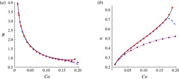
and
 $R$
are related by
 $$\begin{eqnarray}Ca=\frac{1}{4}\sqrt{\frac{3}{2{\rm\pi}}}R^{-5/2}\ln R+O\left(R^{-5/2}\right)\quad \text{as }R\rightarrow \infty .\end{eqnarray}$$
4.4. ‘Stationary’ elliptic tori
Figure 3(b) shows that, for
 $Ca\leqslant 0.16$
, the cross-section of an initially circular torus with
 $R=R_{cr}(Ca)$
approaches an approximately elliptic shape. This section finds ‘stationary’ elliptic tori through the inverse problem outlined in § 4.1.
In the
 $rz$
half-plane in the cylindrical coordinates, the cross-section of an elliptic torus having the volume of a unit sphere can be parametrized by
 $$\begin{eqnarray}r(t)=R+a\cos t,\quad z(t)=b\sin t,\quad b=\frac{2}{3{\rm\pi}Ra},\quad t\in [-{\rm\pi},{\rm\pi}],\end{eqnarray}$$
where
 $R$
and
 $a$
can still be referred to as major and minor torus radii respectively, and
 $b=2/(3{\rm\pi}Ra)$
follows from the volume constraint. In this case,
 $$\begin{eqnarray}\text{div}_{S}\,\boldsymbol{n}(t,{\it\varphi})=\frac{b\left(4aR+\left(5a^{2}+3b^{2}\right)\cos t+\left(b^{2}-a^{2}\right)\cos [3t]\right)}{4(R+a\cos t)\left(a^{2}\sin ^{2}t+b^{2}\cos ^{2}t\right)^{3/2}}.\end{eqnarray}$$
The inverse problem in § 4.1 implies that for each
 $R$
and
 $a$
,
 $Ca$
is expressed by (4.5), and
 $\mathscr{E}_{2}^{2}(u_{n}^{+},w;S)$
with (4.5) is minimized with respect to
 $a$
over the interval
 $[\sqrt{2/(3{\rm\pi}R)},R]$
,
 $$\begin{eqnarray}a(R)=\text{argmin}_{a}\mathscr{E}_{2}^{2}\left(u_{n}^{\infty },w;S\right)-\frac{\left(\displaystyle \oint _{S}w(\boldsymbol{x})u_{n}^{\infty }(\boldsymbol{x})v(\boldsymbol{x})\,\text{d}S_{x}\right)^{2}}{\mathscr{E}_{2}^{2}\left(v,w;S\right)}\quad \text{subject to }\sqrt{\frac{2}{3{\rm\pi}R}}\leqslant a\leqslant R,\end{eqnarray}$$
which is found by the golden section method. (The golden section method requires identification of an interval on which a minimized function is convex. In this case, an appropriate subinterval of
 $[\sqrt{2/(3{\rm\pi}R)},R]$
can be identified visually by plotting the minimized function.) Optimal
 $Ca$
, denoted as
 $Ca(R)$
, is then determined by (4.5) with given
 $R$
and
 $a(R)$
found as in (4.18).
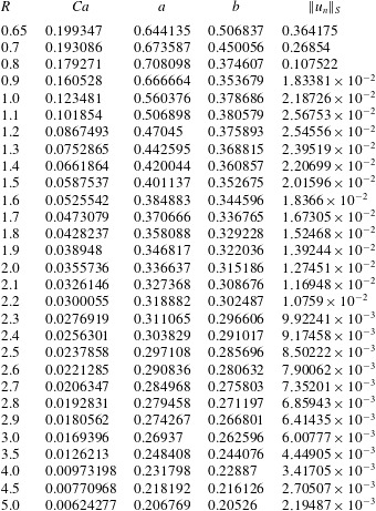
Table 5 presents
 $Ca(R)$
,
 $a(R)$
and
 $b(R)=2/(3{\rm\pi}\,R\,a(R))$
for ‘stationary’ elliptic tori found from the inverse problem (4.18) for
 $R\in [0.65,5]$
with
 $w=r^{-1}$
and also provides the mean absolute value
 $\Vert u_{n}\Vert _{S}$
defined by (3.8). The increase of
 $\Vert u_{n}\Vert _{S}$
for
 $Ca>0.16$
is quite noticeable. Figure 14 compares the parameters
 $R$
and
 $a$
as functions of
 $Ca$
for ‘stationary’ elliptic tori found from the inverse problem (4.18) with
 $w=r^{-1}$
(dashed curves) and for (3.7) which fits the cross-sections of the stationary toroids with
 $K=1$
(fitted ellipses, red circles) and with
 $K=5$
(solid curves). For
 $Ca\leqslant 0.16$
, all three curves are visually indistinguishable. The triangles correspond to
 $(Ca(R),R)$
with
 $Ca(R)$
determined by (4.9) for ‘stationary’ circular tori, which approximate the stationary toroids quite well for
 $Ca\leqslant 0.05$
.


5. Discussion
5.1. Dynamics
Simulations of the dynamic deformation for a toroidal drop with an initially circular cross-section show that for each
 $Ca<Ca_{cr}$
, there is a critical major radius
 $R_{cr}$
, and there are three deformation regimes corresponding to
 $R<R_{cr}$
,
 $R=R_{cr}$
and
 $R>R_{cr}$
, see figure 3. In each case, the cross-section initially deforms to a shape close to elliptic. When the initial
 $R>R_{cr}$
, the torus expands indefinitely with
 $R$
increasing exponentially in time. This result can be anticipated, since the tensile shrinking force resisting the expansion of the torus, being of
 $O(R^{-1})$
, decays as
 $R\rightarrow \infty$
, and, hence, the torus cross-section moves almost with the outer flow. The expansion rate
 $$\begin{eqnarray}\frac{\text{d}R}{\text{d}{\it\tau}}\sim R\quad \Longrightarrow \quad R\sim \exp ({\it\tau}).\end{eqnarray}$$
Thus, the large-
 $R$
asymptotic expansion rate depends neither on the initial conditions nor on the capillary number, which is reflected by the same slope of the
 $R({\it\tau})$
curves in figures 2 and 5. Moreover, as
 $R$
increases, the toroidal drop gradually assumes a circular cross-section. This reflects the ever growing local curvature, of
 $O(R^{1/2})$
, of the cross-section perimeter which renders the tension forces there increasingly dominant.
For
 $Ca<0.16$
and
 $R<R_{cr}$
, the torus collapses towards the axis of symmetry. Again, initially, the cross-section assumes a shape that resembles an ellipse. However, when the radius of the inner interface shrinks, the local surface surrounding the gap at the axis of symmetry flattens into a cylindrical shape (see, e.g., figure 4), reflecting the local viscous stress that develops at this gap due to the need to drain the suspending viscous fluid from this diminishing region. With time, a circular depression develops about the symmetry plane
 $z=0$
– an indication that some of the outer fluid remains trapped within this dimpled shape, and that the contact (and perhaps coalescence) of the torus may occur above and below
 $z=0$
.
5.2. High
$Ca$

For
 $Ca$
sufficiently close to
 $Ca_{cr}$
, e.g.
 $Ca\in [0.19,0.2]$
, the resulting dynamics has a different character. When the torus expands, the initial circular cross-section deforms to a highly asymmetric egg shape which extends further until it is sufficiently far from the axis of symmetry, at which stage the cross-section gradually becomes circular again (see, e.g., figure 6). For
 $Ca=0.2$
, the extended inner circular tip of the torus collapses to complete contact. When
 $Ca\gg Ca_{cr}$
, the drop expansion reveals yet another pattern. For
 $Ca=0.5$
and two different values of initial
 $R$
, figure 7 shows that after an initial short-lived deformation of the cross-section into an elliptical shape, the drop keeps on flattening and attains a very thin shape that might be susceptible to collapse and disintegration. If this does not happen, with further toroidal expansion, a small circular cross-section is regained. These examples reflect the dominance of the distorting viscous stresses upon the interfacial tension.
5.3. Instability and breakup
The dynamics of toroidal drop deformations, simulated in § 3.1, admits several scenarios where the drop may break up. When the inner circle of the torus shrinks during an inward collapse and approaches the axis of symmetry, coalescence may occur either at the symmetry plane
 $z=0$
or far from it when a dimpled inner region exists. In such cases, the toroidal drop may regain a simply connected shape or form a multiphase drop if a portion of the outer fluid is captured into the drop. In another scenario that can lead to a breakup, the drop has a highly flattened cross-section – the drop in figure 7(b) (
 $Ca=0.5$
,
 $R=0.8$
) is likely to disintegrate into many small droplets. Furthermore, highly expanded tori with shrinking circular cross-sections can experience instabilities in the form of varicose waves, which can result in drop breakup as well. Thus, all of this described dynamics, be it collapse or expansions, can lead to a destruction of the toroidal drop in finite time.
5.4. Stationary solutions
For
 $Ca<Ca_{cr}$
and
 $R=R_{cr}(Ca)$
, where
 $R_{cr}(Ca)$
should be determined very accurately for
 $Ca\lesssim Ca_{cr}$
, drop dynamics simulations could maintain a stationary toroid with almost elliptic cross-section for a relatively long time (see § 3.1), which suggests that (2.10) has doubly connected solutions. However, such stationary shapes cannot be maintained in this way forever because of the inherent instability: they will either expand or contract following any tiny deviation of
 $R({\it\tau})$
from its equilibrium value. As a result, the anticipated experimental realization may prove difficult. Nevertheless, as § 3.3 shows, unstable stationary toroids with the error
 $\Vert u_{n}\Vert _{S}$
on the scale of
 $10^{-3}$
exist as long as
 $Ca<Ca_{cr}$
. (‘Stationary’ circular and elliptic tori that minimize an error functional exist for considerably higher values of
 $Ca$
, although the corresponding error is much larger.) Figure 10 shows that the cross sections of stationary toroids are quite close to circular for
 $Ca\leqslant 0.05$
, whereas figures 9(a) and 11 suggest that they are almost perfect ellipses for
 $Ca\leqslant 0.16$
. Remarkably, the curve
 $(Ca(R),R)$
with
 $Ca(R)$
determined by (4.9) for ‘stationary’ circular tori predicts
 $(Ca,R_{cr}(Ca))$
quite accurately for all
 $Ca$
up to
 $Ca_{cr}$
(see figure 13), and the ‘stationary’ elliptic tori found from the inverse problem (4.18) with
 $w=r^{-1}$
are visually indistinguishable from the corresponding stationary toroids obtained in drop dynamics simulations for
 $Ca\leqslant 0.16$
. Figures 9(b) and 12 show that when
 $Ca\rightarrow Ca_{cr}$
, the elliptic cross-section is distorted to that of an extended egg, with the sharper end pointing towards the axis of symmetry.
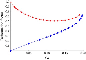
The Taylor deformation factor
 $D=(R_{max}-z_{max})/(R_{max}+z_{max})$
for a simply connected stationary shape (diamonds) and for a toroidal stationary shape (circles) as a function of
 $Ca$
. In the ‘circles’ curve, the short dashed curve at
 $Ca\sim 0$
does not follow from computations, but reflects the assumption that
 $R_{max}\rightarrow \infty$
as
 $Ca\rightarrow 0$
.

5.5. Solution non-uniqueness
The problem (2.1)–(2.5) with
 ${\mathcal{U}}_{n}=0$
, which corresponds to the stationary states of the torus, is identical to the one for steady shapes of a simply connected oblate drop embedded in the same linear compressional flow; see Zabarankin et al. (Reference Zabarankin, Smagin, Lavrenteva and Nir2013). To describe the two cases in one plot, we redefine the Taylor deformation parameter by the ratio of the maximum half-thickness and the maximum radius at the drop meridian perimeter,
 $$\begin{eqnarray}D=\frac{R_{max}-z_{max}}{R_{max}+z_{max}},\end{eqnarray}$$
see figure 15, where the lower and upper curves correspond to the simply connected oblate drop (
 ${\it\lambda}=1$
) and the doubly connected toroidal drop respectively, which were found for approximately the same range of
 $Ca$
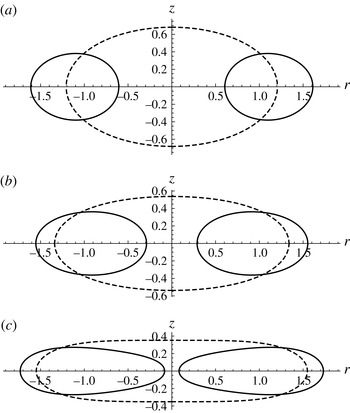
. Figure 16 shows the cross-sections of the simply connected and toroidal stationary shapes existing for the same value of
 $Ca$
. The solution non-uniqueness arises from the fact that the drop interface, being unknown, enters equations (2.1)–(2.5) nonlinearly.
Cross-sections of the stable simply connected stationary-state shape (dashed curves) and of the unstable toroidal stationary-state shape (solid curves) for (a)
 $Ca=0.1$
, (b)
 $Ca=0.15$
and (c)
 $Ca=0.19$
.

Acknowledgements
A.N. and O.M.L. acknowledge partial support by the Israel Science Foundation (grant no. ISF/327.17) and thank I. Smagin for writing the Fortran code used for the dynamic simulations presented in § 3.1. O.M.L. also acknowledges the support of the Israel Ministry of Immigrant Absorption.
Appendix A. Axisymmetric velocity field representation
Suppose that the regions
 $V^{+}$
and
 $V^{-}$
, occupied by the drop and the fluid respectively and having a common boundary
 $S$
(interface), are axisymmetric. Let
 $(r,{\it\varphi},z)$
be a system of cylindrical coordinates with the basis
 $(\boldsymbol{e}_{r},\boldsymbol{e}_{{\it\varphi}},\boldsymbol{e}_{z})$
, where the
 $z$
-axis is the axis of revolution, and let
 ${\mathcal{D}}^{\pm }$
be the cross sections of
 $V^{\pm }$
in the meridional
 $rz$
half-plane (
 $r\geqslant 0$
). The regions
 ${\mathcal{D}}^{\pm }$
are closed and their common boundary (cross-section of
 $S$
) is assumed to be a positively oriented curve
 $\ell$
, which is either closed (as for a toroid) or open with the ends lying on the
 $z$
-axis (as for a spheroid). In the axisymmetric case (the
 $z$
-axis is the axis of revolution),
 $\boldsymbol{u}^{\infty }=r\,\boldsymbol{e}_{r}-2z\,\boldsymbol{e}_{z}$
and
 $\boldsymbol{u}^{\pm }$
are given by (3.1). The components
 $u_{r}^{\pm }$
and
 $u_{z}^{\pm }$
in (3.1) are independent of the angular coordinate
 ${\it\varphi}$
and can be represented by (3.5a,b) in Zabarankin et al. (Reference Zabarankin, Smagin, Lavrenteva and Nir2013), which are unified in the form
 $$\begin{eqnarray}u_{z}^{\pm }(r,z)+\text{i}\,u_{r}^{\pm }(r,z)=\frac{1\pm 1}{2}(\text{i}\,r-2z)+\frac{1}{Ca}\int _{\ell }\text{div}_{S}\,\boldsymbol{n}({\it\tau})(K_{1}({\it\zeta},{\it\tau})\,\text{d}{\it\tau}-K_{2}({\it\zeta},{\it\tau})\,\overline{\text{d}{\it\tau}})\end{eqnarray}$$
for
 ${\it\zeta}\in {\mathcal{D}}^{\pm }$
, where
 ${\it\zeta}=r+\text{i}\,z$
and
 ${\it\tau}=r_{1}+\text{i}\,z_{1}$
, with
 $\text{i}=\sqrt{-1}$
,
 $\overline{\text{d}{\it\tau}}$
is the complex conjugate of
 $\text{d}{\it\tau}$
, and the kernels
 $K_{1}$
and
 $K_{2}$
are defined by
 $$\begin{eqnarray}\displaystyle & \displaystyle K_{1}({\it\zeta},{\it\tau})=\frac{1}{2{\rm\pi}\text{i}}\frac{z-z_{1}-{\displaystyle \frac{\text{i}}{2}}(r-r_{1})}{{\it\tau}-{\it\zeta}}\frac{\left|{\it\tau}+\overline{{\it\zeta}}\right|}{2r}\left\{({\it\chi}^{2}({\it\zeta},{\it\tau})-1)\mathbb{K}({\it\chi}({\it\zeta},{\it\tau}))+\mathbb{E}({\it\chi}({\it\zeta},{\it\tau}))\right\},\hspace{-10.00002pt} & \displaystyle \nonumber\\ \displaystyle & & \displaystyle\end{eqnarray}$$
 $$\begin{eqnarray}\displaystyle & \displaystyle K_{2}({\it\zeta},{\it\tau})=\frac{1}{2{\rm\pi}\text{i}}\frac{z-z_{1}-{\displaystyle \frac{\text{i}}{2}}(r+r_{1})}{\overline{{\it\tau}}+{\it\zeta}}\frac{\left|{\it\tau}+\overline{{\it\zeta}}\right|}{2r}\left\{\mathbb{K}({\it\chi}({\it\zeta},{\it\tau}))-\mathbb{E}({\it\chi}({\it\zeta},{\it\tau}))\right\}, & \displaystyle\end{eqnarray}$$
with
 ${\it\chi}^{2}({\it\zeta},{\it\tau})=4r_{1}r|{\it\tau}+\overline{{\it\zeta}}|^{-2}$
and with
 $\mathbb{K}({\it\chi}({\it\zeta},{\it\tau}))$
and
 $\mathbb{E}({\it\chi}({\it\zeta},{\it\tau}))$
being complete elliptic integrals of the first and second kinds respectively. The complex form of (A 1) is due to the fact that (A 1) was obtained through the generalized Cauchy integral formula for
 $r$
-analytic functions, see Zabarankin (Reference Zabarankin2008, Reference Zabarankin2012). In this case, the pressure and vorticity in
 ${\mathcal{D}}^{\pm }$
are represented by the formulae (3.10) and (3.9) respectively in Zabarankin & Nir (Reference Zabarankin and Nir2011).