1.1. Motivation

This article investigates how carrying a beneficial genetic mutation influences the quantity of transmitted genome, in a population of sexually reproducing hermaphroditic individuals. Building on previous works [Reference Coron and Le Jan5, Reference Coron and Le Jan6], we consider a population, represented by a biparental Moran model, of haploid individuals whose genome is a random and balanced mixture of their two parents’ genomes. Initially, a proportion a of individuals carry a mutation that increases their life expectancy and thus their genetic contribution to the population. Our goal is to quantify the effect of selection strength on the genetic composition of the population in the limit of large population size, and more specifically to determine the impact of the advantage conferred by the mutation on the genetic contribution of ancestors. Our approach could be used, for instance, to estimate the strength of selection in a population composed of two types of individuals (e.g. coming from two different source populations), using admixture data, as is the object of [Reference Fortes-Lima, Laurent, Thouzeau, Toupance and Verdu13, Reference Verdu and Rosenberg26].

Our paper focuses on two major phenomena in population genetics: on the one hand, the impact of selection on genome structure, which has been the subject of numerous studies, and on the other hand, the biparental transmission of the genome, which has been relatively little studied so far. Biparental genealogies and genetics have received some interest, notably in [Reference Chang3, Reference Derrida, Manrubia and Zanette8, Reference Gravel and Steel14], in which the time to more recent common ancestors and ancestors’ weights are investigated for the Wright–Fisher biparental model. In [Reference Coron and Le Jan5], we studied the asymptotic law of the contribution of an ancestor to the genome of the present-time population within a neutral genetic framework. In [Reference Lambert, Miró Pina and Schertzer19], the authors studied the asymptotic structure of the genome of individuals in a population experiencing biparental haploid reproduction, while in [Reference Pfaffelhuber and Wakolbinger22] the authors studied the biparental transmission of transposable elements in diploid populations. The monoparental Moran model with selection at birth has received some interest, notably in [Reference Etheridge and Griffiths10], which studies its dual coalescent, and [Reference Kluth and Baake16], which studies allele fixation probabilities and ancestral lines. The impact of selection on genetic transmission has also been studied using the concept of an ancestral selection graph, introduced in [Reference Krone and Neuhauser18], that notably led to the articles [Reference Baake, Lenz and Wakolbinger1, Reference Cordero4, Reference Fearnhead11, Reference Kluth, Hustedt and Baake17, Reference Lenz, Kluth, Baake and Wakolbinger20, Reference Taylor25] dealing with ancestor type distribution in populations modeled by monoparental bi-type Wright–Fisher or Moran models with mutation and selection, and using the lookdown construction. Finally, a few articles combine selection and biparental pedigree. The articles [Reference Matsen and Evans21] and [Reference Barton and Etheridge2] study the link between pedigree, individual reproductive success, and genetic contribution, while in [Reference Coron and Le Jan6] we studied the expectation of the asymptotic contribution to the genome of a biparental population of a mutant subject to infinite selection.

Studying the dynamics of genome transmission during the fixation period of an advantageous allele is linked to studying genetic hitchhiking, which is done notably in [Reference Etheridge, Pfaffelhuber and Wakolbinger9, Reference Schweinsberg and Durrett23] for haploid individuals and in [Reference Stephan, Song and Langley24] for diploid individuals. Genetic hitchhiking is a phenomenon through which the dynamics of the frequency of an allele is influenced by the dynamics of genes under selection that are close to this first allele, or at least on the same DNA strand. This phenomenon intrinsically relies on the spatial structure of the genome, and on the fact that two pieces of genomes that are close to each other on the genome have a large probability of being transmitted together during reproduction. In this article we study the transmission of the genome of advantaged individuals, while assuming that the genome is composed of infinitely many independent loci (which is obviously a strong simplification). In some sense, we study the weakest form of genetic hitchhiking, in which pieces of genome are linked only through the fact that they are present in the same individual and are transmitted through the same pedigree, which is itself shaped by the transmission of advantageous alleles. The form and role of the pedigree on unlinked neutral loci during a selective sweep is also investigated using simulations in [Reference Wakeley, King and Wilton27] for populations of diploid individuals.

Note: A manuscript bearing a similar title to the present work has been deposited on arXiv and is not intended for publication. It contains the proof of a weaker convergence statement, based on properties of the discrete model, some of which have not been included in the present work.

1.2. Model

Following the framework of previous papers [Reference Coron and Le Jan5, Reference Coron and Le Jan6], we model the dynamics of a population of N haploid individuals using a biparental two-type discrete-time Moran model with viability selection and no mutation. Time will be represented by the set $\mathbb{Z}_+=\{0,1,\ldots\}$ of non-negative integers.

Specifically, we consider a population of fixed size N in which a mutation at a given locus confers an advantage to individuals carrying it. We assume that selection affects only the death rate of individuals: advantaged individuals have a death weight of 1, while non-advantaged individuals have a death weight of $1+s$ , with $s\gt0$ . At each discrete time step, two individuals are chosen uniformly at random with replacement to be parents and produce one offspring, which replaces a third individual chosen with probability proportional to its death weight (and independently from the two parents, which means that a child can replace its own parent, and also that both parents can be the same individual). This results in a death probability at each time step that is $1+s$ times higher for a non-advantaged individual than for an advantaged individuals, leading to an increased life expectancy and mean offspring number for the latter. The selection parameter s will not depend on N, as is often the case in population genetics literature, and in particular we will not explore the diffusive scalings introduced in [Reference Kimura15].

Genetic transmission follows Mendelian rules, in the sense that at a given locus of the genome, each individual inherits an allele, chosen uniformly at random among the two alleles of its parents. In particular, the transmission of advantage to offspring is characterized by Mendelian transmission at one locus. We refer to the parent that transmits a copy of its gene at the locus under selection as the ‘mother’ and the other parent as the ‘father’. An individual is therefore advantaged if and only if its mother is advantaged. The limiting case where s is infinite (i.e. only non-advantaged individuals can die) has been studied in a previous paper [Reference Coron and Le Jan6], and comparisons to this work will be provided later on. As in [Reference Coron and Le Jan5, Reference Coron and Le Jan6], recombination is not considered. We indeed focus on the probability for a gene sampled at the present time to originate from a given ancestor, which can be seen as the proportion of genome transmitted by this ancestor if the genome is seen as a set of infinitely many independent loci.

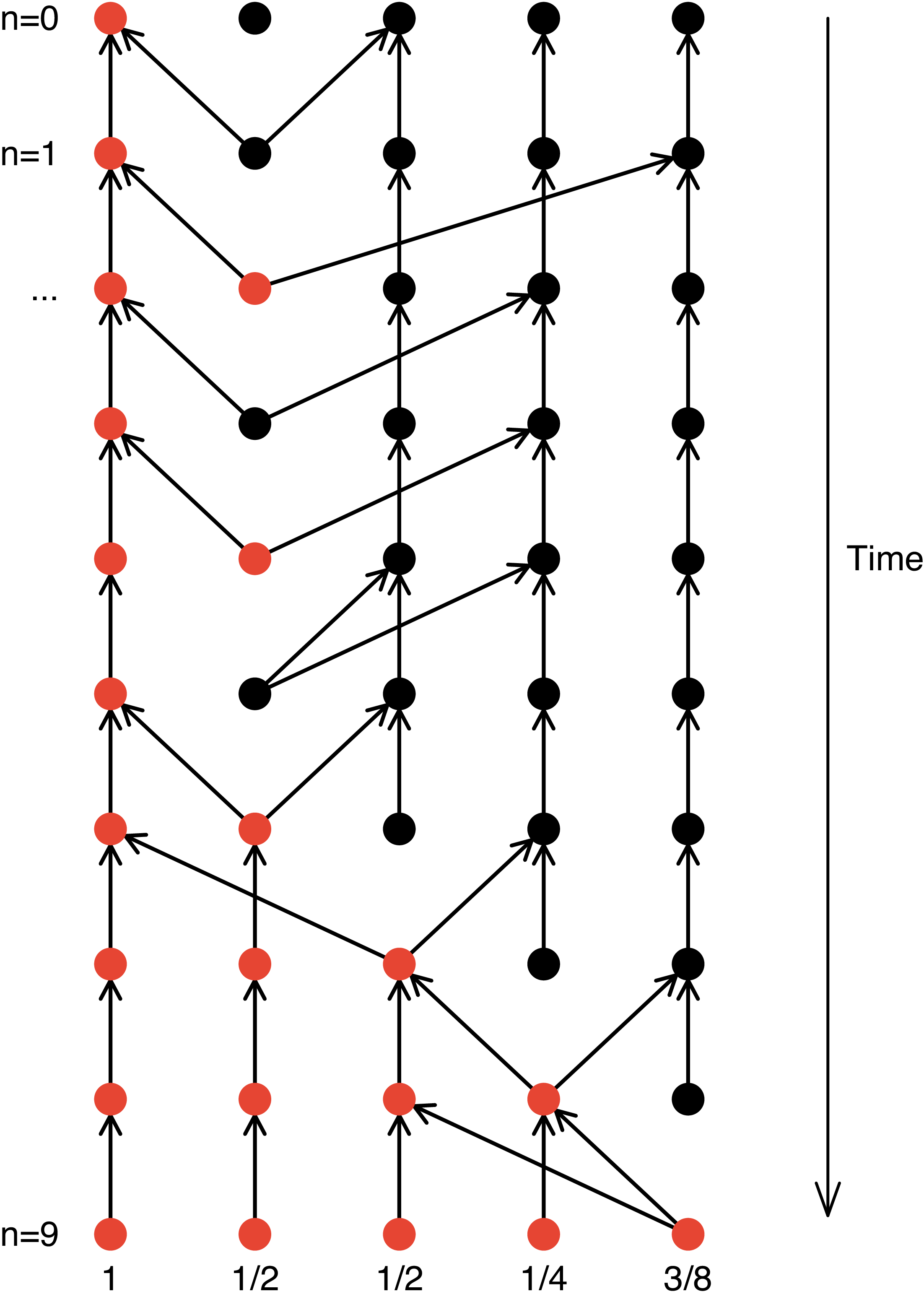
Let us denote by $I=\{1,2,\ldots,N\}$ the sites in which individuals live (which is simply a way to number individuals at each time step), and denote by $(\mu_n,\pi_n,\kappa_n)\in I^3$ the respective positions of the mother, father, and dying individual at time step $n\in\mathbb{Z}_+$ . As in [Reference Coron and Le Jan5], the reproduction dynamics described above defines an oriented random graph on $I\times\mathbb{Z}_+$ (as shown in Figure 1), denoted by G, representing the pedigree of the population, such that between time n and time $n+1$ , two arrows are drawn from $(\kappa_n,n+1)$ to $(\pi_n,n)$ and $(\mu_n,n)$ respectively and $N-1$ arrows are drawn from $(i,n+1)$ to (i, n) for each $i\in I\setminus\{\kappa_n\}$ . Note that individuals are now also characterized by their advantage: advantaged individuals are represented in red in Figure 1. We denote by $\mathcal{Y}_n\subset \{1,\ldots,N\}$ the set of advantaged individuals at time n. We also define by $(\mathcal{F}_n,n\in\mathbb{Z}_+)$ the filtration associated to the whole population dynamics, i.e. $\mathcal{F}_n=\sigma(\mathcal{Y}_0,\{\mu_l,\pi_l,\kappa_l, l\lt n\})$ for any $n\in\mathbb{Z}_+$ . The filtration $(\mathcal{F}_n,n\in\mathbb{Z}_+)$ notably includes the filtration associated to the stochastic process $(\mathcal{Y}_n)_{n\in\mathbb{Z}_+}$ . Note that the pedigree is characterized only by the sequence $((\{\mu_n,\pi_n\},\kappa_n))_{n\in\mathbb{Z}_+}$ , which is not a Markov chain, due to selection. We denote by $\{\mathcal{G}_n,n\in\mathbb{Z}_+\}$ with $\mathcal{G}_n=\sigma(\{\{\mu_l,\pi_l\},\kappa_l,l\lt n\})$ its associated filtration.

1.3. Ancestors’ genetic weights

To investigate the impact of selection on the genetic composition of the population, we consider a second locus that is far enough from the locus under mutation that the genome is assumed to be transmitted independently at these two loci. We then sample an individual in the population at time n and consider the genealogy of its gene at this second locus, i.e. the sequence of ancestral individuals through which this gene was transmitted, at all times $0\leq n-k\leq n$ . This genealogy, denoted by $(X^{(n)}_k, n-k)_{0\leq k\leq n}$ , is a symmetric random walk on the pedigree G. A particularly interesting element is the number $X_n^{(n)}$ that gives the position of the initial ancestor of the sampled gene.

The key object in this model, as introduced in [Reference Coron and Le Jan5], is therefore the sequence of random variables $((W_n(i,j))_{1\leq i,j\leq N})_{n\geq 0}$ defined by

(1) \begin{align} W_n(i,j)=\mathbb{P}\big(X^{(n)}_n=j\mid X^{(n)}_0=i,\mathcal{G}_n\big).\end{align}

In words, the quantity $W_n(i,j)$ is the probability, given the pedigree before time n, $\mathcal{G}_n$ , that any gene of individual i living at time n comes from the ancestor j, living at time 0. It is a deterministic function of the random graph G between time 0 and time n and does not depend on the advantage status of individuals in the pedigree (although the pedigree itself depends on this status). More formally, $W_n(i,j)=\mathbb{P}(X^{(n)}_n=j\mid X^{(n)}_0=i,\mathcal{F}_n)$ .

If the genome is very large and the evolution of distant genes sufficiently decorrelated, we can expect this quantity to be close to the proportion of genes of individual i that come from individual j. For this reason we refer to this quantity as the genetic weight at time n of ancestor j in the genome of individual i (see Figure 1 for an illustration). We define the genetic weight of ancestor j at time n as the sum $\sum_{i=1}^NW_n(i,j)$ .

Figure 1.

This figure represents simultaneously the pedigree G and the set of advantaged individuals, over ten time steps in a population of five individuals. The time orientation is from past to future and arrows materialize gene flow between individuals, represented backwards in time. Advantaged individuals are represented in red. The numbers at the bottom give the probability that a gene sampled in each of the individuals come from the initially advantaged individual. In this example the genetic weight of the initially advantaged individual (i.e. N times the probability, given the pedigree, that a gene sampled uniformly at time $n=9$ comes from this individual at time $n=0$ ) is equal to $21/8=1+1/2+1/2+1/4+3/8$ .

1.4. Main result

Recall that $\mathcal{Y}_n\subset I$ denotes the set of advantaged individuals at time n, and let $Y_n$ be its cardinality, i.e. the number of advantaged individuals at time n. Our goal is to investigate the impact of selection on the weight of ancestors, and notably to study the probability that a gene sampled in the population at the present time originated from an advantaged individual.

To this end we introduce the quantities

\begin{align*}U_n=\sum_{l\in\mathcal{Y}_n}\sum_{l'\in\mathcal{Y}_0} W_n(l,l'), \quad V_n=\sum_{l\notin\mathcal{Y}_n}\sum_{l'\in\mathcal{Y}_0} W_n(l,l').\end{align*}

$U_n$ (resp. $V_n$ ) will be called the total genetic weight of initially advantaged ancestors among advantaged (resp. disadvantaged) individuals at time n; it gives the quantity of genome coming from the initially advantaged ancestors and carried by advantaged (resp. disadvantaged) individuals, assuming that each individual carries a quantity of genome equal to 1. The quantity $U_n\in[0,N]$ (resp. $V_n\in[0,N]$ ) is equal to $Y_n$ (resp. $N-Y_n$ ) times the probability, knowing the pedigree, that a gene sampled uniformly among advantaged (resp. non-advantaged) individuals at time n originates from an initially advantaged individual. More formally, as long as $Y_n\notin\{0,N\}$ , if we denote by $\mathcal{U}(A)$ the uniform law on a discrete set A,

\begin{align*}\frac{U_n}{Y_n}&=\mathbb{P}\big(X_n^{(n)}\in \mathcal{Y}_0\mid X^{(n)}_0\sim\mathcal{U}(\mathcal{Y}_n),\mathcal{G}_n\big), \\[5pt] \frac{V_n}{N-Y_n}&=\mathbb{P}\big(X_n^{(n)}\in\mathcal{Y}_0\mid X^{(n)}_0\sim\mathcal{U}(I\setminus\mathcal{Y}_n),\mathcal{G}_n\big).\end{align*}

We denote by $T_k$ the first hitting time of any integer k lying between 0 and N by the Markov chain $(Y_n)_{n\in\mathbb{N}}$ . Then the two quantities

\begin{align*}\frac{U_{T_N}}{N}\mathbf{1}_{\{T_N\lt\infty\}}=\frac{U_{T_N}}{Y_{T_N}}\mathbf{1}_{\{T_N\lt\infty\}}\quad\text{and}\quad\frac{V_{T_0}}{N}\mathbf{1}_{\{T_0\lt\infty\}}=\frac{V_{T_0}}{N-Y_{T_0}}\mathbf{1}_{\{T_0\lt\infty\}}\end{align*}

represent the proportion of genome of the population coming from initially advantaged individuals once the mutation is fixed or has disappeared, respectively. They indeed give the probability that a gene sampled uniformly from the population, once the latter has become monomorphic, originates from an advantaged individual (see Figure 1 for an example starting with one advantaged individual, and fixation of this type).

After the time $\inf(T_0,T_N)$ the population continues to evolve according to the neutral model studied in [Reference Coron and Le Jan5]. Note finally that although $W_n$ is a $\mathcal{G}_n$ -measurable function, the genetic weights $U_n$ and $V_n$ are not, since the pedigree alone does not give the advantage status of individuals. The precise dynamics of all these stochastic processes will be given in the next section, but our brief introduction so far suffices to state our main result.

Theorem 1. Let $Z_n=({Y_n}/{N},{U_n}/{N},{V_n}/{N})_{n\in\mathbb{N}}$ and $a\in(0,1)$ . If $Y_0=\lfloor aN\rfloor$ then, for any $c\in\mathbb{R}_+$ ,

(2) \begin{align} \textrm{sup}_{0\leq t\leq c}\|Z_{\lfloor Nt\rfloor}-z_t\|\underset{N\rightarrow\infty}{\longrightarrow}0 \end{align}

in probability, where $(z_t)_{t\geq0}=(y_t,u_t,v_t)_{t\geq0}$ satisfies

\begin{align*}\left\{ \begin{aligned} y_t &= F^{-1}\bigg(\frac{a^{1+s}}{1-a}\exp\!(st)\bigg), \quad\textit{where $F\colon x\mapsto\dfrac{x^{1+s}}{1-x}$ maps $[0,1)$ onto $[0,\infty)$}, \\[5pt] u_t &= y_t\frac{a^{({1+s})/{2s}}}{(1-a)^{{1}/{2s}}}\bigg[\frac{(1-y_t)^{{1}/{2s}}}{y_t^{({1+s})/{2s}}}+\int_a^{y_t}\frac{(1-x)^{{1}/{2s}}}{x^{({1+s})/{2s}}}\bigg[\frac{1}{2}+\frac{1}{2s}\frac{1}{1-x}\bigg]\,{\mathrm{d}} x\bigg], \\[5pt] v_t &= (1-y_t)\frac{a^{({1+s})/{2s}}}{(1-a)^{{1}/{2s}}}\int_a^{y_t}\frac{(1-x)^{{1}/{2s}}}{x^{({1+s})/{2s}}}\bigg[\frac{1}{2}+\frac{1}{2s}\frac{1}{1-x}\bigg]\,{\mathrm{d}} x. \end{aligned}\right.\end{align*}

This result gives the convergence of the trajectory of the stochastic process $(Z_{\lfloor Nt\rfloor})_{0\leq t\leq c}$ for any $c\gt0$ towards an explicit solution of a dynamical system. In particular, it gives the genetic contribution of the initially advantaged individuals in compact time intervals under a large population size assumption. More precisely, it gives the limiting dynamics of the proportion of advantaged individuals ( $Y_{\lfloor Nt\rfloor}/N$ ), and of the proportion of genome coming from advantaged individuals carried respectively by advantaged ( $U_{\lfloor Nt\rfloor}/N$ ) and disadvantaged ( $V_{\lfloor Nt\rfloor}/N$ ) individuals. In Section 2 we will see that the limiting dynamics of the proportion of advantaged individuals results from an autonomous differential equation,

\begin{align*}y'=\frac{sy(1-y)}{y+(1+s)(1-y)}.\end{align*}

This differential equation, driven by the selection parameter s, can be compared to that obtained for the classical (monoparental) Moran model, for which the proportion z of advantaged individuals under a similar scaling satisfies $z'=sz(1-z)$ (as can be seen in [Reference Cordero4, Proposition 3.1], for instance). The difference between the two equations lies in the biparental Mendelian transmission versus the clonal transmission. A simple and unsurprising comparison between the two models is that the proportion of advantaged individuals increases more slowly in the biparental Mendelian model, since $y+(1+s)(1-y)\gt1$ . Note that if the initial proportion of advantaged individuals ${Y_0}/{N}$ is equal to $\lfloor aN\rfloor$ then $\mathbb{P}(T_N\lt T_0)\rightarrow 1$ when N goes to infinity (Proposition 4). The following corollary gives, under a large population approximation, the genetic weight of the initially advantaged ancestors, initially assumed to be in proportion a, when this proportion reaches any level $b\gt a$ .

Corollary 1. Let $a\lt b\in(0,1)$ . If $Y_0=\lfloor aN\rfloor$ then

\begin{align*} \frac{U_{T_{\lfloor bN\rfloor}}}{N}\mathbf{1}_{\{T_{\lfloor bN\rfloor\}}\lt\infty} \underset{N\rightarrow\infty}{\longrightarrow} b\frac{a^{({1+s})/{2s}}}{(1-a)^{{1}/{2s}}}\bigg[\frac{(1-b)^{{1}/{2s}}}{b^{({1+s})/{2s}}} + \int_a^{b}\frac{(1-x)^{{1}/{2s}}}{x^{({1+s})/{2s}}}\bigg[\frac{1}{2}+\frac{1}{2s}\frac{1}{1-x}\bigg]\, {\mathrm{d}} x\bigg] \end{align*}

in probability.

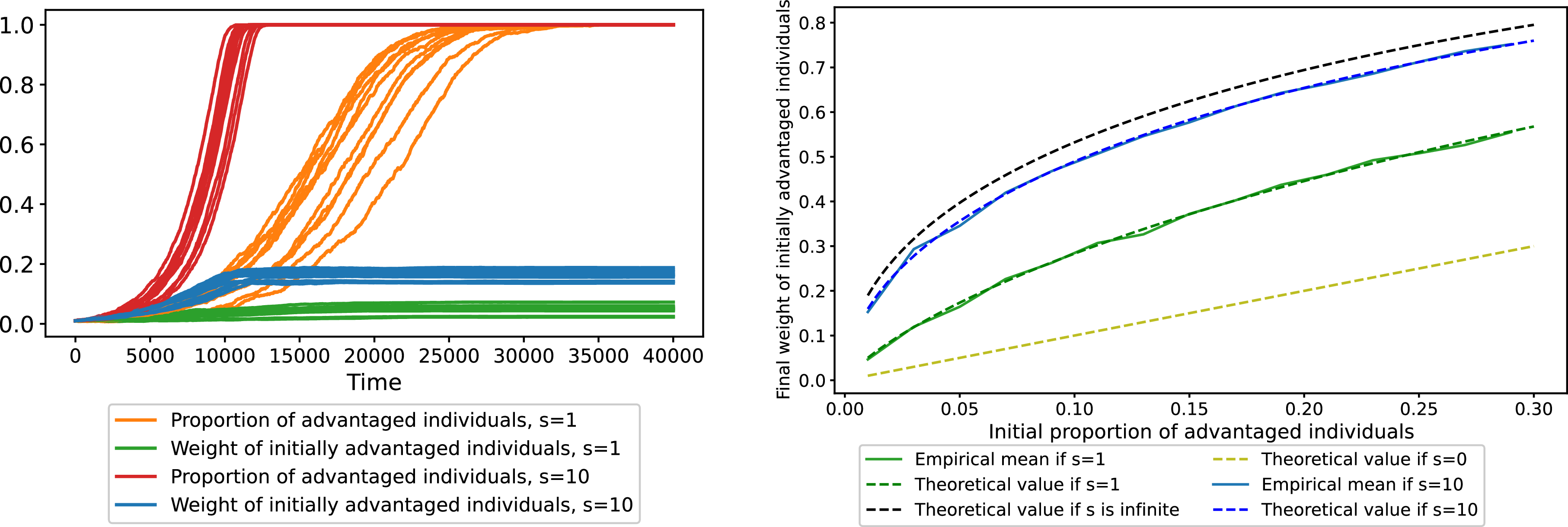
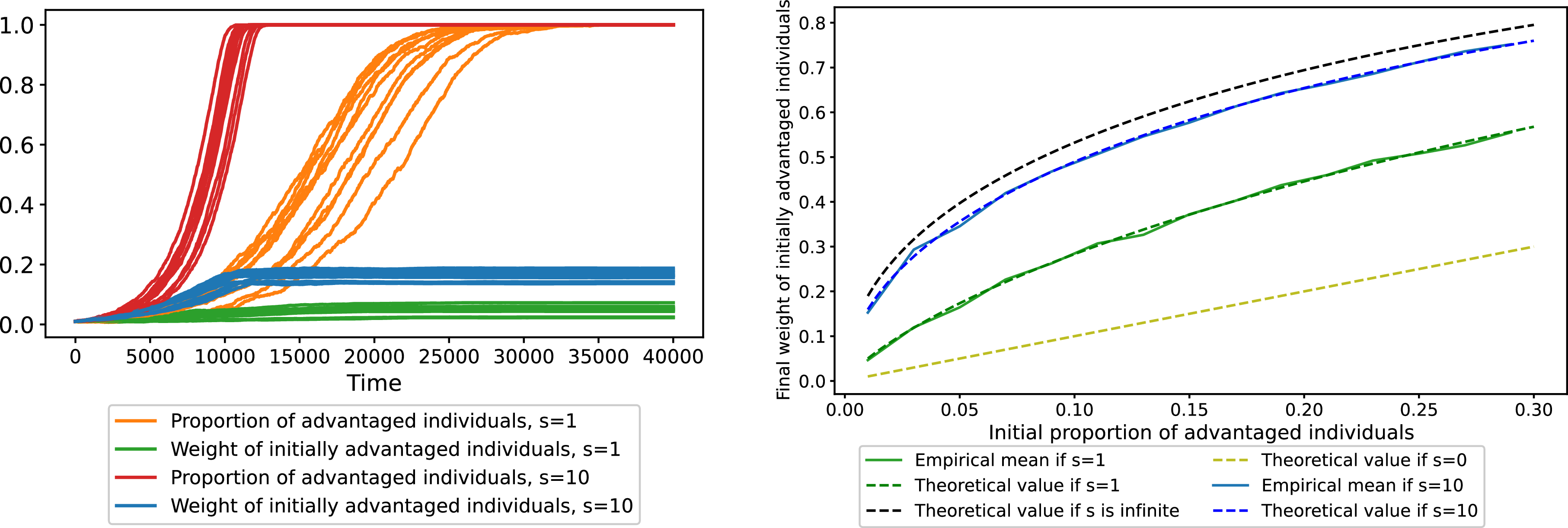
We think that this still holds true for $b=1$ , but proving it would necessitate a finer study of the variance of $U_n$ (see [Reference Coron and Le Jan7] for the proof of the convergence of the expectation of ${U_{T_{N}}}/{N}$ ). As an example, if $s=1$ then Corollary 1 tells us that if 1% of the individuals are initially advantaged, then they will on average end up being responsible for approximately 5% of the whole population’s genome (instead of 1% in the neutral case where $s=0$ ). Note also that the limit given in Corollary 1 is non-decreasing in s, and we can see that it converges to $2\sqrt{a}-a$ as $s\uparrow \infty$ and b converges to 1. This result can also be retrieved from [Reference Coron and Le Jan6], in which we focused on the case where $s=\infty$ . In particular, for large selection strength s, if only 1% of the individuals are initially advantaged, they will on average be responsible for approximately 19% of the population’s genome. Theorem 1 and Corollary 1 are illustrated in Figure 2.

Figure 2.

Left: For $N=1000$ and $a=1\%$ we plot ten realizations of the dynamics of the proportion of advantaged individuals (in red for $s=10$ and in orange for $s=1$ ) and the genetic weight of initially advantaged individuals (in blue for $s=10$ and in green for $s=1$ ). Right: For different values of the initial proportion of advantaged individuals, we plot for $s=1$ (in green) and for $s=10$ (in blue) the mean of the weight at time $n=40\,000$ of the initially advantaged individuals over ten simulations. We also give the associated theoretical predictions, as well as the theoretical predictions for $s=0$ (in yellow) and for infinite s (in black).

2.1. A few Markovian properties

We begin by presenting a series of results that shed light on various aspects of the dynamics of the process under consideration, and notably the interplay between the set and number of advantaged individuals, the pedigree, and the genetic weights of ancestors.

2.1.1. Number and set of advantaged individuals

We first focus on the set and number of advantaged individuals, whose dynamics happen to be particularly simple. Recall that $\mu_n\in I$ is the site of the mother (the parent that transmits advantage) at time step n, while $\kappa_n\in I$ is the site of the individual that is killed at step n. These notations combined with the modeling framework described in Section 1.2 immediately give the following result.

Proposition 1. The stochastic process $(\mathcal{Y}_n)_{n\in\mathbb{Z}_+}$ is a Markov chain such that

Proof. If the mother is chosen among advantaged individuals then by the definition of the model described in Section 1.2, the site $\kappa_n$ is added to (or remains in) the set of advantaged individuals. If the mother is chosen among non-advantaged individuals then the site $\kappa_n$ is removed from the set of advantaged individuals if it was present in this set.

As a consequence we have the next result.

Proposition 2. The stochastic process $(Y_n)_{n\in\mathbb{Z}_+}$ is a Markov chain such that if $Y_n=k\in \{0,1,\ldots,N\}$ , then $Y_{n+1}\in\{k-1,k,k+1\}$ and

\begin{align*} \mathbb{P}(Y_{n+1}=k-1\mid Y_n=k) & = p_k\times\frac{1}{2+s}, \\[5pt] \mathbb{P}(Y_{n+1}=k+1\mid Y_n=k) & = p_k\times\frac{1+s}{2+s}, \\[5pt] \mathbb{P}(Y_{n+1}=k\mid Y_n=k) & = 1-p_k, \end{align*}

where

\begin{align*} p_k & = \frac{k(N-k)}{N(({1}/({2+s}))k + (({1+s})/({2+s}))(N-k))} \\[5pt] & = \frac{1}{(({1}/({2+s}))({N}/({N-k})) + (({1+s})/({2+s})({N}/{k}))}. \end{align*}

This Markov chain is absorbed in 0 and in N.

Proof. As summarized in Proposition 1, the number of advantaged individuals is increased by 1 if the mother is advantaged while the dying individual is disadvantaged, which gives

\begin{align*} \mathbb{P}(Y_{n+1}=k+1\mid Y_n=k) & = \frac{k}{N}\times\frac{(1+s)(N-k)}{k+(1+s)(N-k)} \\[5pt] & = \frac{1+s}{2+s}\times \frac{k(N-k)}{N(({1}/({2+s}))k+(({1+s})/({2+s}))(N-k))}. \end{align*}

Similarly, the number of advantaged individuals is decreased by 1 if the mother is disadvantaged while the dying individual is advantaged, which gives

\begin{align*} \mathbb{P}(Y_{n+1}=k-1\mid Y_n=k) & = (N-k)/N\times\frac{k}{k+(1+s)(N-k)} \\[5pt] & = \frac{1}{2+s}\times \frac{k(N-k)}{N(({1}({2+s}))k+(({1+s})/({2+s}))(N-k))}. \end{align*}

Finally, the number of advantaged individuals remains the same if the mother and replaced individual have the same advantage status, which gives

\begin{align*} \mathbb{P}(Y_{n+1}=k\mid Y_n=k) & = \frac{k}{N}\frac{k}{k+(1+s)(N-k)}+\frac{N-k}{N}\frac{(1+s)(N-k)}{k+(1+s)(N-k)} \\[5pt] & = \frac{k^2+(1+s)(N-k)^2}{N(k+(1+s)(N-k))}=1-\frac{(2+s)k(N-k)}{N(k+(1+s)(N-k))}=1-p_k. \end{align*}

As $p_0=p_N=0$ , this gives that the states 0 and N are absorbing.

The previous result implies that the skeleton of the Markov chain $(Y_n)_{n\in\mathbb{Z}_+}$ has a particularly simple dynamics. More precisely, let $\tau_0=0$ and $H_0=Y_0=Y_{\tau_0}$ . Now, for any $l\in\mathbb{Z}_+^*$ , if $H_l\notin\{0,N\}$ let $\tau_{l+1}=\inf\{n\gt\tau_l\mid Y_n\neq H_l\}$ and $H_{l+1}=Y_{\tau_{l+1}}$ . If $Y_{\tau_l}\in\{0,N\}$ let $H_{l+1}=H_l$ . Then, from Proposition 2, we have the following.

Proposition 3. The stochastic process $(H_l)_{l\in\mathbb{Z}_+}$ is a simple random walk absorbed in $\{0,N\}$ : for any $l\in\mathbb{Z}_+$ such that $H_l\notin\{0,N\}$ ,

\begin{align*} \mathbb{P}(H_{l+1}=H_{l}+1) = \frac{1+s}{2+s}, \quad \mathbb{P}(H_{l+1}=H_{l}-1)=\frac{1}{2+s}, \end{align*}

and if $H_l\in\{0,N\}$ , $H_{l+1}=H_l$ . We denote by $S_k$ the first hitting time of $k\in\{0,1,\ldots,N\}$ by the random walk H.

This result allows us to prove very simply the first item of the following proposition.

Proposition 4. Let $a\in(0,1)$ . If $Y_0=\lfloor aN\rfloor$ , then

1. (i) The fixation probability of advantaged individuals satisfies $\mathbb{P}(T_N\lt T_0)\underset{N\rightarrow\infty}{\longrightarrow} 1$ .

2. (ii) Let $b\in [a,1)$ . There exists $C\gt0$ (depending on b) such that $\mathbb{P}(T_{\lfloor bN\rfloor}\gt N C)\rightarrow 0$ when N goes to infinity.

Proof. We recall that $S_k$ is the first hitting time of $k\in\{0,1,\ldots,N\}$ by the biased random walk $(H_l)_{l\in\mathbb{Z}_+}$ . Note that $T_N\lt T_0$ if and only if $S_N\lt S_0$ . Then (i) follows from Proposition 3 and from a classical result on ‘gambler’s ruin’ (see, for example, [Reference Feller12, Chap. XIV-1]). Now, let us turn our attention to (ii). The proof is decomposed into two parts: we first prove the result for the absorbed biased random walk $(H_l)_{l\in\mathbb{Z}_+}$ , i.e. we prove that for any $b\in[a,1)$ there exists a constant $K\gt0$ such that $\mathbb{P}(S_{\lfloor bN\rfloor}\gt N K)\rightarrow 0$ when N goes to infinity. Second, we prove that the Markov chain $(Y_n)_{n\in\mathbb{Z}_+}$ cannot stay for a long time at each position, by noting that the parameters $p_k=\mathbb{P}(Y_{n+1}\neq Y_n\mid Y_n=k)$ are bounded from below when the Markov chain $(Y_n)_{n\in\mathbb{Z}_+}$ stays away from $\varepsilon N$ , which occurs with high probability. We conclude using the Bienaymé–Chebyshev inequality.

More formally, we bound the probability of interest as follows. For any $C, K\gt0$ ,

(3) \begin{align} \mathbb{P}(T_{\lfloor bN\rfloor}\gt CN) & \leq \mathbb{P}(T_{\lfloor bN\rfloor}\gt CN,S_{\lfloor \varepsilon N\rfloor} \geq S_{\lfloor bN\rfloor},S_{\lfloor bN\rfloor}\leq KN) \nonumber \\[5pt] & \quad + \mathbb{P}(S_{\lfloor bN\rfloor}\gt KN) + \mathbb{P}(S_{\lfloor \varepsilon N\rfloor}\lt S_{\lfloor bN\rfloor}), \end{align}

and we control the three terms of the right-hand side of this equation. For the last one, note that for any $\varepsilon\lt a$ ,

\begin{align*} \mathbb P(S_{\lfloor bN\rfloor}\lt S_{\lfloor \varepsilon N\rfloor}) = \frac{(1+s)^{\lfloor \varepsilon N\rfloor-\lfloor a N\rfloor}-1}{(1+s)^{\lfloor \varepsilon N\rfloor-\lfloor bN\rfloor}-1} \rightarrow 1 \end{align*}

as N goes to infinity. For the second term, let us introduce a random walk $\tilde{H}$ which has the same transition probabilities and starting point $\lfloor aN\rfloor$ as the random walk H but is not absorbed in $\{0,N\}$ , i.e. which is such that $\mathbb{P}(\tilde{H}_{l+1}=\tilde{H}_{l}+1)=({1+s})/({2+s})$ and $\mathbb{P}(\tilde{H}_{l+1}=\tilde{H}_{l}+1)={1}/({2+s})$ whatever value $\tilde{H}_l$ takes in $\mathbb{Z}$ . We have, for any $K\gt0$ ,

(4) \begin{align} \mathbb{P}(S_{\lfloor bN\rfloor}\gt KN)\leq\mathbb{P}(H_{KN}\lt\lfloor bN\rfloor) & \leq \mathbb{P}(H_{KN}=0)+\mathbb{P}(0\lt\tilde{H}_{KN}\lt\lfloor bN\rfloor)) \nonumber \\[5pt] & \leq \mathbb{P}(H_{KN}=0)+\mathbb{P}(\tilde{H}_{KN}\lt bN)). \end{align}

Now recall that $H_0=Y_0=\lfloor aN\rfloor$ . Therefore $\mathbb{P}(H_{KN}=0)=\mathbb{P}(S_0\leq KN)\leq \mathbb{P}(S_0\lt\infty)\rightarrow 0$ as N goes to infinity from the same gambler’s ruin result as before. Also, by the law of large numbers, $({\tilde{H}_{KN}-\lfloor aN\rfloor})/{N}$ converges to $({s}/({2+s}))K$ when N goes to infinity. Hence $\mathbb{P}(\tilde{H}_{KN}\lt\lfloor bN\rfloor)$ goes to 0 when N goes to infinity as soon as $K\gt{(b-a)(2+s)}/{s}$ . Therefore, from (4), $\mathbb{P}(S_{\lfloor bN\rfloor}\gt KN)$ goes to 0 when N goes to infinity if K is large enough.

We finally consider the first term of the right-hand side of (3). We know that

\begin{align*} \mathbb{P}(Y_{n+1}\neq Y_n\mid Y_n=k) = p_k = \frac{k(N-k)}{N(({1}/({2+s}))k+(({1+s})/({2+s}))(N-k))}= f(k/N), \end{align*}

with

\begin{align*}f(x)=\frac{1}{({1}/({2+s}))({1}/({1-x}))+(({1+s})/({2+s}))({1}/{x})}.\end{align*}

Since $f'(0+)\gt0$ , $f(0)=0$ , and $f\gt0$ on (0, b], there exists $\varepsilon\gt0$ such that $p_k\gt p_{\lfloor \varepsilon N\rfloor}$ for all $\lfloor \varepsilon N\rfloor\leq k\leq \lfloor bN\rfloor$ if N is large enough. Moreover, as $f'(0)=({2+s})/({1+s})$ , $p_{\lfloor \varepsilon N\rfloor}\gt\varepsilon$ if N is large enough. Now, on $T_k\lt\infty$ , $T_k=\sum_{i=0}^{S_k-1}L_i $ , with the $L_i$ being, conditionally on H, independent geometric random variables with parameter $p_{H_i}^{}$ . Therefore

\begin{align*} \mathbb{P}(T_{\lfloor bN\rfloor}\gt CN \mid S_{\lfloor \varepsilon N\rfloor} \geq S_{\lfloor bN\rfloor},S_{\lfloor bN\rfloor}\leq KN) \leq \mathbb{P}\Bigg(\sum_{i=0}^{KN}L_i\gt CN\Bigg), \end{align*}

and therefore

\begin{align*} \mathbb{P}(T_{\lfloor bN\rfloor}\gt CN, S_{\lfloor \varepsilon N\rfloor} \geq S_{\lfloor bN\rfloor},S_{\lfloor bN\rfloor}\leq KN) \leq \mathbb{P}\Bigg(\sum_{i=0}^{KN}L_i\gt CN\Bigg). \end{align*}

Now, recall that any geometric random variable of parameter $p'_2\gt p'_1$ can be decomposed into the sum of M independent geometric random variables of parameter $p'_1$ , M being an independent geometric random variable of parameter $p'_1/p'_2$ . We can infer that

\begin{align*} \mathbb{P}(T_{\lfloor bN\rfloor}\gt CN, S_{\lfloor \varepsilon N\rfloor} \geq S_{\lfloor bN\rfloor},S_{\lfloor bN\rfloor}\leq KN) \leq \mathbb{P}\Bigg(\sum_{i=0}^{KN}D_i\gt CN\Bigg), \end{align*}

where the $D_i$ are independent geometric random variables with parameter $p_{\lfloor \varepsilon N\rfloor}$ . Since the expectation and the variance of $\sum_{i=0}^{KN}D_i$ are respectively smaller than ${KN}/{\varepsilon}$ and ${KN}/{\varepsilon^2}$ , we conclude using the Bienaymé–Chebyshev inequality if we take C larger than ${K}/{\varepsilon}$ .

Note that the previous result can be extended to the case where $Y_0/N$ converges in probability to $a\in(0,1)$ .

Ancestors’ genetic weights. Let us now focus on ancestors’ weights. Due to selection, the sequence of ancestors’ weights $((W_n(i,j)_{1\leq i,j\leq N})_{n\in\mathbb{Z}_+}$ is not a Markov chain. However, the pair $((W_n(i,j)_{1\leq i,j\leq N},\mathcal{Y}_n)_{n\in\mathbb{Z}_+}$ is, and satisfies the following property.

Lemma 1. The sequence $(W_n,\mathcal{Y}_n)_{n\in\mathbb{Z}_+}$ is a Markov chain, with transition rules

(5)

(6) \begin{align} W_{n+1}(i,j) & = \begin{cases} W_n(i,j) & \text{if $i\neq \kappa_n$}, \\[5pt] \dfrac12{W_n(\mu_n,j)+W_n(\pi_n,j)} & \text{if $i=\kappa_n$,} \end{cases} \end{align}

where $\mu_n$ and $\pi_n$ are drawn uniformly in $1,\ldots,N$ , and $\kappa_n$ is such that

\begin{align*}\mathbb{P}(\kappa_n=i)=\frac{1+s\mathbf{1}_{\{i\notin\mathcal{Y}_n\}}}{Y_n+(1+s)(N-Y_n)}\end{align*}

for all $i\in\{1,\ldots,N\}$ .

Proof. Equation (5) is equivalent to the result stated in Proposition 2, and (6) is a consequence of the model presented in Section 1.2 and the definition in (1).

Now recall the definitions of the two key quantities,

\begin{align*}U_n=\sum_{l\in\mathcal{Y}_n}\sum_{l'\in\mathcal{Y}_0} W_n(l,l'), \quad V_n=\sum_{l\notin\mathcal{Y}_n}\sum_{l'\in\mathcal{Y}_0} W_n(l,l'),\end{align*}

and note that $U_0=Y_0$ and $V_0=0$ . From now on we consider the sequence of the rescaled triplets $Z_n=({Y_n}/{N},{U_n}/{N},{V_n}/{N})\in[0,1]^3$ and denote by $(\mathcal{F}^Z_n,n\geq0)$ its natural filtration. We also denote by $\mathcal{C}^2([0,1]^3)$ the set of real-valued twice continuously differentiable functions on $[0,1]^3$ . Our first aim in this section is to present the dynamics of this stochastic process and to prove that when the population size goes to infinity, this stochastic process converges to the solution of a dynamical system that can be explicitly solved.

First, the following proposition follows from Lemma 1.

Proposition 5. The sequence $(Z_n)_{n\in\mathbb{Z}_+}=({Y_n}/{N},{U_n}/{N},{V_n}/{N})_{n\in\mathbb{Z}_+}$ (which is not Markovian) is such that

(7) \begin{align} Z_{n+1} & = Z_n + \frac{1}{N}\Bigg[ \Bigg(1,\sum_{l'\in\mathcal{Y}_0}\frac{W_n(\mu_n,l')+W_n(\pi_n,l')}{2}, \sum_{l'\in\mathcal{Y}_0}-W_n(\kappa_n,l')\Bigg) \mathbf{1}_{\{\mu_n\in\mathcal{Y}_n,\kappa_n\notin\mathcal{Y}_n\}} \nonumber \\[5pt] & \qquad\; + \Bigg({-}1, -\sum_{l'\in\mathcal{Y}_0}W_n(\kappa_n,l'), \sum_{l'\in\mathcal{Y}_0}\frac{W_n(\mu_n,l')+W_n(\pi_n,l')}{2}\Bigg) \mathbf{1}_{\{\mu_n\notin\mathcal{Y}_n,\kappa_n\in\mathcal{Y}_n\}} \nonumber \\[5pt] & \qquad\; + \Bigg(0,\sum_{l'\in\mathcal{Y}_0}\frac{W_n(\mu_n,l')+W_n(\pi_n,l')}{2} - \sum_{l'\in\mathcal{Y}_0}W_n(\kappa_n,l'),0\Bigg) \mathbf{1}_{\{\mu_n\in\mathcal{Y}_n,\kappa_n\in\mathcal{Y}_n\}} \nonumber \\[5pt] & \qquad\; + \Bigg(0,0,\sum_{l'\in\mathcal{Y}_0}\frac{W_n(\mu_n,l')+W_n(\pi_n,l')}{2} - \sum_{l'\in\mathcal{Y}_0}W_n(\kappa_n,l')\Bigg) \mathbf{1}_{\{\mu_n\notin\mathcal{Y}_n,\kappa_n\notin\mathcal{Y}_n\}}\Bigg]. \end{align}

In particular, since $\sum_jW_n(i,j)\leq1$ , $\|Z_{n+1}-Z_n\|\leq \sqrt{3}/N$ for all $n\geq0$ , and

(8) \begin{align} \mathbb{E}\big(Z_{n+1}-Z_n\mid\mathcal{F}^Z_n\big) & = \frac{1}{N}\bigg(\frac{sY_n/N(1-Y_n/N)}{Y_n/N+(1+s)(1-Y_n/N)}, \nonumber \\[5pt] & \qquad\quad \frac{U_n}{2N} + \frac{U_n+V_n}{2N}\frac{Y_n}{N} - \frac{U_n/N}{Y_n/N+(1+s)(1-Y_n/N)}, \nonumber \\[5pt] & \qquad\quad \frac{V_n}{2N} + \frac{U_n+V_n}{2N}\bigg(1-\frac{Y_n}{N}\bigg) - \frac{(1+s)V_n/N}{Y_n/N+(1+s)(1-Y_n/N)}\bigg). \end{align}

Proof. Equation (7) follows from the model described in Section 1.2 (i.e. from Lemma 1), and (8) follows from (7) and from the fact that $\mu_n$ and $\pi_n$ are uniformly chosen in $\{1,\ldots,N\}$ and $\kappa_n\in\mathcal{Y}_n$ with probability ${Y_n}/[{Y_n+(1+s)(N-Y_n)}]$ . For example, the first term ${U_n}/{2N}$ in the second coordinate of the right-hand side of (8) is equal to

\begin{align*}\mathbb{E}\Bigg(\sum_{l'\in\mathcal{Y}_0} \frac{W_n(\mu_n,l')}{2}\mathbf{1}_{\{\mu_n\in\mathcal{Y}_n\}}\Bigg),\end{align*}

which appears when adding the first and third terms in (7).

From the previous proposition we will derive the convergence, as the population size goes to infinity, of the stochastic sequence $(Z_{\lfloor N\rfloor})_N$ , towards a solution of the following dynamical system:

(9) \begin{align} \begin{cases} y' = \dfrac{sy(1-y)}{y+(1+s)(1-y)}, \\[3mm] u' = \bigg[\dfrac{u}{2}+\dfrac{u+v}{2}y-\dfrac{u}{y+(1+s)(1-y)}\bigg], \\[3mm] v' = \bigg[\dfrac{v}{2}+\dfrac{u+v}{2}(1-y)-\dfrac{(1+s)v}{y+(1+s)(1-y)}\bigg], \end{cases}\end{align}

which is the first element of Theorem 1.

2.2. Dynamical system

We first determine this solution of the system.

Proposition 6. The differential equation (9) admits the unique solution $z_t\;:\!=\;(y_t,u_t,v_t)_{t\geq0}$ starting from (a, a, 0) with $a\in(0,1)$ . This solution satisfies

(10) \begin{align} \left\{ \begin{aligned} y_t & = F^{-1}\bigg(\frac{a^{1+s}}{1-a}\exp\!(st)\bigg), \quad \textit{where $F\colon x\rightarrow\frac{x^{1+s}}{1-x}$ maps $[0,1)$ onto $[0,\infty)$}, \\[5pt] u_t & = y_t\frac{a^{({1+s})/{2s}}}{(1-a)^{{1}/{2s}}}\bigg[ \frac{(1-y_t)^{{1}/{2s}}}{y_t^{({1+s})/{2s}}} + \int_a^{y_t}\frac{(1-x)^{{1}/{2s}}}{x^{({1+s})/{2s}}} \bigg[\frac{1}{2}+\frac{1}{2s}\frac{1}{1-x}\bigg]\,{\mathrm{d}} x\bigg], \\[5pt] v_t & = (1-y_t)\frac{a^{({1+s})/{2s}}}{(1-a)^{{1}/{2s}}} \int_a^{y_t}\frac{(1-x)^{{1}/{2s}}}{x^{({1+s})/{2s}}} \bigg[\frac{1}{2}+\frac{1}{2s}\frac{1}{1-x}\bigg]\,{\mathrm{d}} x. \end{aligned}\right. \end{align}

Proof. We initially focus on the first differential equation of (9), which happens to be autonomous and easily solvable:

(11) \begin{align} \frac{{\mathrm{d}} y_t}{{\mathrm{d}} t}=\frac{sy_t(1-y_t)}{y_t+(1+s)(1-y_t)}=\frac{sy_t(1-y_t)}{1+s(1-y_t)}\;=\!:\;m(y_t), \end{align}

with $y_0=a$ . Since the function m is Lipschitz continuous on [0, 1], from the Picard–Lindelöf (or Cauchy–Lipschitz) theorem, this ordinary differental equation admits a unique solution starting at $a\in[0,1]$ . Since $m(0)=m(1)=0$ , this solution is simply constant if $a\in\{0,1\}$ , and if $a\in(0,1)$ then this solution is such that $y_t\in(0,1)$ for all t, and the differential equation (11) can then also be written as

\begin{align*}\frac{{\mathrm{d}} y_t}{{\mathrm{d}} t}\bigg[\frac{1+s}{y_t}+\frac{1}{1-y_t}\bigg]=s.\end{align*}

Noting that $({1+s})/{y}$ and ${1}/({1-y})$ are the respective derivatives of $y\rightarrow(1+s)\ln(y)$ and $y\rightarrow-\ln(1-y)$ gives us that the solution to this equation starting from a satisfies

(12) \begin{align} \frac{y_t^{1+s}}{1-y_t}=\frac{a^{1+s}}{1-a}\exp\!(st)\in[0,\infty) \quad\text{for all $t\geq0$}. \end{align}

Let F be the function such that $F(x)={x^{1+s}}/({1-x})$ for all $x\in[0,1)$ . The function F is strictly increasing on [0, 1) and sends [0, 1) onto $[0,+\infty)$ . Therefore, since $a\in[0,1)$ , (12) gives

\begin{align*}y_t= F^{-1}\bigg(\frac{a^{1+s}}{1-a}\exp\!(st)\bigg) \quad \text{for all $t\geq0$},\end{align*}

which is the first equation of (10).

Note that in particular we have

(13) \begin{align} \exp\!(t/2) = \exp\!(st)^{{1}/{2s}} = \bigg(F(y_t)\frac{1-a}{a^{1+s}}\bigg)^{{1}/{2s}} = \frac{y_t^{({1+s})/{2s}}}{(1-y_t)^{{1}{2s}}}\frac{(1-a)^{{1}/{2s}}}{a^{({1+s})/{2s}}}. \end{align}

This formula will be used at the end of the proof.

Let us now come back to the whole differential equation (9). The existence and uniqueness of the solution starting from the initial condition (a, a, 0) again follow from the Cauchy–Lipschitz theorem. This solution $(z_t)_{t\geq0}$ takes values in $[0,1]^3$ . Now, from (9),

\begin{align*} \bigg(\frac{u}{y}\bigg)' = \frac{u'}{y} - u\frac{y'}{y^2} & = \frac{u}{2y} + \frac{u+v}{2} - \frac{u}{y[y+(1+s)(1-y)]} - \frac{usy(1-y)}{y^2[y+(1+s)(1-y)]} \\[5pt] & = \frac{u+v}{2}-\frac{u}{2y}; \end{align*}

similarly,

(14) \begin{align} \bigg(\frac{v}{1-y}\bigg)' & = \frac{v'}{1-y} + v\frac{y'}{(1-y)^2} \nonumber \\[5pt] & = \frac{v}{2(1-y)} + \frac{u+v}{2} - \frac{(1+s)v}{(1-y)[y+(1+s)(1-y)]} + \frac{vsy(1-y)}{(1-y)^2[y+(1+s)(1-y)]} \nonumber \\[5pt] & = \frac{u+v}{2}-\frac{v}{2(1-y)}. \end{align}

Hence,

\begin{align*} \bigg(\frac{u}{y}-\frac{v}{1-y}\bigg)' = -\frac{1}{2}\bigg(\frac{u}{y}-\frac{v}{1-y}\bigg), \end{align*}

which gives that

\begin{align*} \frac{u_t}{y_t} - \frac{v_t}{1-y_t} = \exp\!\bigg({-}\frac{t}{2}\bigg) \end{align*}

since $u_0=y_0$ and $v_0=0$ .

Therefore, considering the quantity $D_t={u_t{\mathrm{e}}^{t/2}}/{y_t}-{v_t{\mathrm{e}}^{t/2}}/({1-y_t})$ , we have

(15) \begin{align} \frac{{\mathrm{d}} D_t}{{\mathrm{d}} t}=0, \quad \text{hence}\ D_t=D_0=1 \quad \text{for all $t\geq0$.} \end{align}

Note that this property is a fundamental characteristic of our model. An analogous version of it was given in [Reference Coron and Le Jan6, (1.7)] in a discrete setting and for infinite selection, and can be extended to the finite selection case (see [Reference Coron and Le Jan7, Proposition 2.6]).

Equation (15) gives

(16) \begin{align} u_t{\mathrm{e}}^{t/2}=y_t\bigg(1+\frac{v_t}{1-y_t}{\mathrm{e}}^{t/2}\bigg) \end{align}

for all $t\geq0$ . Finally, let us set

(17) \begin{align} \beta_t=\frac{v_t}{1-y_t}{\mathrm{e}}^{t/2}. \end{align}

We can express $\beta_t$ as a function of $y_t$ . Indeed, since

\begin{align*}\frac{{\mathrm{d}}\beta_t}{{\mathrm{d}} t}=\frac{u_t+v_t}{2}{\mathrm{e}}^{t/2}\end{align*}

from (14),

\begin{align*} \frac{{\mathrm{d}}\beta_t}{{\mathrm{d}} y_t} = \frac{{{\mathrm{d}}\beta_t}/{{\mathrm{d}} t}}{{{\mathrm{d}} y_t}/{{\mathrm{d}} t}} & = \frac{({u_t+v_t})/{2}{\mathrm{e}}^{t/2}}{{sy_t(1-y_t)}/({y_t+(1+s)(1-y_t)})} \\[5pt] & = \frac{y_t\big[1+({v_t}/({1-y_t})){\mathrm{e}}^{t/2}\big] + v_t{\mathrm{e}}^{t/2}}{{2sy_t(1-y_t)}/({y_t+(1+s)(1-y_t)})} \qquad\qquad\text{(from (16))} \\[5pt] & = \frac{y_t+\beta_t}{{2sy_t(1-y_t)}/({y_t+(1+s)(1-y_t)})}. \end{align*}

So

(18) \begin{align} \frac{{\mathrm{d}}\beta_t}{{\mathrm{d}} y_t} = \frac{\beta_t}{{2sy_t(1-y_t)}/({y_t+(1+s)(1-y_t)})} + \frac{y_t+(1+s)(1-y_t)}{2s(1-y_t)}, \end{align}

and this linear autonomous equation can be solved by variation of parameters. We introduce a function C defined on (0, 1) such that

\begin{align*} \beta_t=C(y_t)\frac{y_t^{({1+s})/{2s}}}{(1-y_t)^{{1}/{2s}}}\quad\text{for all $t\geq0$}. \end{align*}

Then, from (18),

\begin{align*} \frac{{\mathrm{d}} C}{{\mathrm{d}} y}\frac{y^{({1+s})/{2s}}}{(1-y)^{{1}/{2s}}} = \frac{y+(1+s)(1-y)}{2s(1-y)} = \frac{y}{2s(1-y)}+\frac{1+s}{2s}, \end{align*}

and therefore

\begin{align*} \frac{{\mathrm{d}} C}{{\mathrm{d}} y} = \frac{(1-y)^{({1}/{2s})-1}}{2sy^{(({1+s})/{2s})-1}} + \frac{1+s}{2s}\frac{(1-y)^{{1}/{2s}}}{y^{({1+s})/{2s}}}. \end{align*}

Hence, since $\beta_0=0$ and $y_0=a$ ,

\begin{align*} C(y) = \frac{1}{2s}\int_a^{y}\frac{(1-x)^{{1}/{2s}}}{x^{({1+s})/{2s}}}\bigg[\frac{x}{1-x}+1+s\bigg]\,{\mathrm{d}} x & = \frac{1}{2s}\int_a^{y}\frac{(1-x)^{{1}/{2s}}}{x^{({1+s})/{2s}}}\bigg[\frac{1}{1-x}+s\bigg]\,{\mathrm{d}} x \\[5pt] & = \int_a^{y}\frac{(1-x)^{{1}/{2s}}}{x^{({1+s})/{2s}}}\bigg[\frac{1}{2}+\frac{1}{2s}\frac{1}{1-x}\bigg]\,{\mathrm{d}} x, \end{align*}

which gives

\begin{align*} \beta_t = \frac{y_t^{({1+s})/{2s}}}{(1-y_t)^{{1}/{2s}}}\int_a^{y_t}\frac{(1-x)^{{1}/{2s}}}{x^{({1+s})/{2s}}} \bigg[\frac{1}{2}+\frac{1}{2s}\frac{1}{1-x}\bigg]\,{\mathrm{d}} x. \end{align*}

Hence, from (13) and the definition of $\beta_t$ in (17),

\begin{align*} \frac{v_t}{1-y_t} = {\mathrm{e}}^{-{t}/{2}}\beta_t = \frac{a^{({1+s})/{2s}}}{(1-a)^{{1}/{2s}}}\int_a^{y_t}\frac{(1-x)^{{1}/{2s}}}{x^{({1+s})/{2s}}} \bigg[\frac{1}{2}+\frac{1}{2s}\frac{1}{1-x}\bigg]\,{\mathrm{d}} x, \end{align*}

which gives the third equation of (10).

Finally, from (15),

\begin{align*} \frac{u_t}{y_t} = {\mathrm{e}}^{-{t}/{2}}(1+\beta_t) = \frac{a^{({1+s})/{2s}}}{(1-a)^{{1}/{2s}}}\bigg[\frac{(1-y_t)^{{1}/{2s}}}{y_t^{({1+s})/{2s}}} + \int_a^{y_t}\frac{(1-x)^{{1}/{2s}}}{x^{({1+s})/{2s}}}\bigg[\frac{1}{2}+\frac{1}{2s}\frac{1}{1-x}\bigg]\,{\mathrm{d}} x\bigg], \end{align*}

which gives the second equation of (10).

Recall that in the limiting solution $(z_t)_{t\geq0}=(y_t,u_t,v_t)_{t\geq0}$ , $y_t$ is strictly increasing, from $y_0$ to 1 (the function y was used as a time change in the previous proof). For any $b\in[a,1)$ , let us denote by $r_b$ the hitting time of b by $(y_t)_{t\geq0}$ . The limiting dynamical system $(z_t)_{t\geq0}$ then satisfies the following result.

2.3. Convergence

We finally prove that if $Y_0=\lfloor aN\rfloor$ , then for any constant $c\gt0$ the stochastic process $(Z_{\lfloor Nt\rfloor})_{0\leq t\leq c}$ converges, when N goes to infinity, to the solution $(y_t,u_t,v_t)_{0\leq t \leq c}$ of the dynamical system (9), starting from (a, a, 0). Recall that we denoted by $(\mathcal{F}^Z_n,n\geq 0)$ the filtration associated to the stochastic process $(Z_n)_{n\geq 0}$ .

Proof. From Proposition 5, for any $n\in\mathbb{Z}_+$ we obtain that

\begin{align*}Z_{n+1}-Z_n=A_{n+1}+\frac{1}{N}g(Z_n),\end{align*}

where $g(Z_n)=\mathbb{E}(Z_{n+1}-Z_n\mid\mathcal{F}^Z_n)$ is such that

\begin{align*} g(y,u,v) = \bigg(&\frac{y(1-y)s}{y+(1+s)(1-y)}, \\[5pt] & \frac{u}{2}+\frac{u+v}{2}y-\frac{u}{y+(1+s)(1-y)}, \\[5pt] & \frac{v}{2}+\frac{u+v}{2}(1-y)-\frac{(1+s)v}{y+(1+s)(1-y)}\bigg) \end{align*}

for all $(y,u,v)\in[0,1]^3$ , and $A_{n+1}=Z_{n+1}-Z_n-\mathbb{E}(Z_{n+1}-Z_n\mid\mathcal{F}^Z_n)=Z_{n+1}-\mathbb{E}(Z_{n+1}\mid\mathcal{F}^Z_n)$ . Therefore,

(19) \begin{align} Z_n=Z_0+\sum_{k=1}^n A_k+\frac{1}{N}\sum_{k=0}^{n-1} g(Z_k) \end{align}

and the variables $(A_k)_{1\leq k\leq n}$ are the increments of the $\mathcal{F}^Z$ -martingale $(M_n)_{n\geq 0}$ such that $M_n=\sum_{k=1}^nA_k$ for any $n\geq 0$ . Now, from Doob’s martingale inequality, for all $c\gt0$ ,

\begin{align*} \mathbb{E}\big(\textrm{sup}_{0\leq n\leq \lfloor c N\rfloor}(M_n)^2\big) \leq 4\mathbb{E}\big(M_{\lfloor cN\rfloor}^2\big). \end{align*}

Also, from the martingale property,

\begin{align*} \mathbb{E}\big(M_{\lfloor cN\rfloor}^2\big) = \mathbb{E}\Bigg(\Bigg(\sum_{k=1}^{\lfloor cN\rfloor}A_k\Bigg)^2\Bigg) = \mathbb{E}\Bigg(\sum_{k=1}^{\lfloor cN\rfloor}(A_k)^2\Bigg) \leq \frac{12c}{N} \quad \text{as } \|Z_{n+1}-Z_n\|^2 \leq \frac{3}{N^2}, \end{align*}

which gives that $\sup_{0\leq t\leq c}\big\|\sum_{k=1}^{\lfloor Nt\rfloor} A_k\big\| \longrightarrow 0$ in probability when N goes to infinity. Now, from Proposition 6, $z_t=(a,a,0)+\int_{0}^{t}g(z_s)\,{\mathrm{d}} s$ . Therefore, by (19),

\begin{align*} Z_{\lfloor Nt\rfloor} - z_t = \bigg(\frac{Y_0}{N},\frac{Y_0}{N},0\bigg) - (a,a,0) + \sum_{k=1}^{\lfloor Nt\rfloor}A_k + \int_0^t g(Z_{\lfloor Ns\rfloor}) - g(z_s)\,{\mathrm{d}} s + R_N(t), \end{align*}

where $|R_N(t)|\leq {\|g\|_{\infty}}/{N}$ . Now, since the Jacobian of the function g is bounded, there exists $K\in\mathbb{R}_+$ such that $\|g(z)-g(z')\|\leq K\|z-z'\|$ for all $z,z'\in[0,1]^3$ . Hence

\begin{align*} \big\|Z_{\lfloor Nt\rfloor}-z_t\big\| \leq \bigg\|\bigg(\frac{Y_0}{N},\frac{Y_0}{N},0\bigg) - (a,a,0)\bigg\| + \Bigg\|\sum_{k=1}^{\lfloor Nt\rfloor}A_k\Bigg\| + \int_0^t K\|Z_{\lfloor Ns\rfloor}-z_s)\|\,{\mathrm{d}} s + \frac{\|g\|_{\infty}}{N}. \end{align*}

Therefore, by Gronwall’s inequality, for any $t\in[0,c]$ ,

\begin{align*} \big\|Z_{\lfloor Nt\rfloor}-z_t\big\| \leq \Bigg(\bigg\|\bigg(\frac{Y_0}{N},\frac{Y_0}{N},0\bigg) - (a,a,0)\bigg\| + \Bigg\|\sum_{k=1}^{\lfloor Nt\rfloor}A_k\Bigg\| + \frac{\|g\|_{\infty}}{N}\Bigg){\mathrm{e}}^{Kt}, \end{align*}

which gives the result.

Corollary 1 follows directly from Theorem 1, Proposition 4(ii), and Corollary 2(i).