2. LOWER AND UPPER BOUNDS FOR U

In this section we use the method described in Section 1 to establish a new general upper bound for the renewal function U corresponding to a probability distribution F on [0,∞). To avoid unnecessary trivialities, we assume throughout that F(0) = 0, although it should be clear that the method applies with minor modifications if F has a mass at the origin. Moreover, we will assume that F is not concentrated on one point.

Theorem 2.1: For x ≥ 0, an upper bound for the renewal function is given by

Moreover, this bound is better than Lorden's for all x such that

The last relation is always true at least on an interval [0,a) with 0 < a ≤ ∞.

Proof: Inserting Lorden's bound given in (1) into the renewal equation (8) gives

A simple integration by parts yields

and the bound in (9) follows immediately from the last two relations.

In order to compare U₁(x) with U_L(x), let Δ(x) = U_L(x) − U₁(x). Then, for Δ(x), we have

and, therefore, U₁(x) ≤ U_L(x) if and only if (10) holds, as asserted.

Finally, it is clear that Δ(0) = μ₂ /μ² − 1, which is strictly positive since F is nondegenerate. Since Δ is a continuous function, we have Δ(x) > 0, at least in a neighborhood near zero. █

Marshall [13] used a similar approach to establish an upper bound of the form

where

is the mean residual life (MRL) function associated with F and the supremum above is taken over all t with F(t) > 0. A disadvantage of the last bound is that it cannot be used for distributions with unbounded MRL, such as IMRL distributions with lim_t→∞ m(t) = ∞. However, as demonstrated by Marshall [13], one advantage of the method is that it can be used recursively, by inserting the successive bounds in (8), and this also can be done with the bound in (9).

A direct comparison of the upper bound (9) to the lower bound (7) reveals that, on using both of them, we can provide an interval estimation for U(x) of length μ₂ F(x)/μ².

Moreover, it is worth noting that if the distribution F in Theorem 2.1 is NBUE, then

(i.e. condition (10) holds for all x). Therefore, in this case, U₁(x) is uniformly better than Lorden's bound U_L(x).

On the other hand, if (10) is true in a neighborhood of zero (0 ≤ x < a), we can write

and taking into account that the mean residual lifetime can be expressed as

we obtain

This leads to the double inequality

which offers a necessary condition for (10) to hold on the interval 0 ≤ x < a.

Example 1: Let F be exponential with mean 1. Then the renewal function U(x) equals U(x) = 1 + x. Lorden's bound turns out to be U_L(x) = 2 + x, and the new bound is

Example 2: Consider a Weibull distribution with survival function

When γ ≥ 1, the distribution is NBUE, so in view of the above remark, we have a = ∞ in the theorem. Thus, we consider an example where γ < 1, so that the improvement of U₁(x) over Lorden's bound holds on a bounded interval [0,a). Taking τ = 3 and γ = ½, we see that U_L(x) = 6 + 9x/2, and some straightforward calculations yield that the MRL function equals

Note that

, so that m(x) is smaller than μ₂ /μ in the interval

and larger than μ₂ /μ in the interval

.

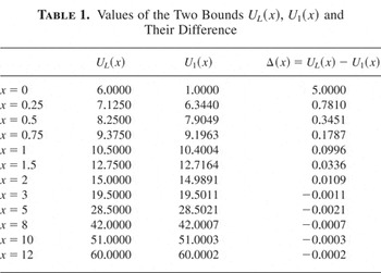
Table 1 presents the values of the two bounds U₁(x) and U_L(x) and their difference, Δ(x) = U_L(x) − U₁(x), for various values of x. Lorden's bound performs poorly for small values of x; notice in particular that Δ(0) = 5 and that for small values of x, say x ≤ 1, there is a substantial improvement of U₁(x) over U_L(x). On the other hand, for values of

, when U_L is better, the magnitude of Δ(x) is always smaller than 3 × 10⁻³.

Values of the Two Bounds UL(x), U1(x) and Their Difference

Example 3: We have seen earlier that if F is NBUE, then condition (10) holds, so that a = ∞ in Theorem 2.1. Is the NBUE condition necessary for a = ∞ in the theorem? The answer is negative, as elucidated by the following example.

Consider a lifetime distribution F with density f (x) given by

It is easily checked that the MRL function corresponding to F is

where Erf denotes the error function. Note that although F has two NBUE parts, it is not a NBUE distribution itself. For a NBUE distribution, it holds that m(x) ≤ m(0) for all x, whereas here, for example, m(1) = 1.5 and m(0) = 0.89. Further, one can verify that μ = 1.2986 and μ₂ = 3.2073, so that μ₂ /μ = 2.47. On noting that the maximum of the MRL function is achieved at x = 1, with m(1) = 1.5, we have shown that m(x) ≤ μ₂ /μ for all x, which, in turn, yields that condition (10) in Theorem 2.1 holds uniformly on the nonnegative half-axis.

Condition (10) requires m(x) to be bounded above by μ₂ /μ, a fact turning U₁(x) to a uniform improvement of Lorden's bound. At this point it is natural to ask whether an alternative upper bound could be established if m(x) was simply bounded, not necessarily by the quantity μ₂ /μ. The next proposition gives an affirmative answer to this, providing a much more flexible bound than U₁(x). Note also that in the case of a MRL that is bounded below, a lower bound for U(x) is deduced.

Proposition 2.2: Let a life distribution F be such that its MRL function is bounded above (below) by a constant r; that is,

for some 0 < a ≤ ∞. Then for the renewal function associated with F and for x ∈ [0,a), it holds that

Proof: We mention first the well-known fact that the solution of (6) is given by

(see e.g. Feller [10, XI]). Further, since U has a unit mass at zero, (14) can be rewritten as

Since m(x) = μF_e(x)/F(x), the condition m(x) ≤ (≥)r for x ∈ [0,a) implies that F_e(x) ≤ (≥)rF(x)/μ, and applying this on the integral term of the right-hand-side series, we obtain

for x ∈ [0,a), as asserted. █

If the life distribution F is NBUE (NWUE), then the MRL function is bounded above (below) by μ for all x ∈ [0,∞). Thus, we arrive at the following result, which is an improvement over (3).

Corollary 2.3: If F is NBUE (NWUE), then

Note that Proposition 2.2 is of much wider applicability than Corollary 2.3. First, the corollary applies only when F is NBUE (NWUE), whereas Proposition 2.2 is in force for the much larger class of distributions whose mean residual life is bounded above (below). Next, condition (13) is only required to hold on a finite interval, not on the whole of the nonnegative half-axis; therefore, the proposition is in fact applicable to all distributions whose MRL is bounded in an interval [0,a) for some a > 0. This implies, in particular, that for most distributions of interest, both a lower and an upper bound are available.

Before closing this section, we state two additional lower bounds for U(x) that do not require any assumptions on the underlying distribution F.

Insert first (7) into (8) to obtain

and then use (11) to deduce the more appealing expression

This can also be obtained as an immediate consequence of the fact that the solution of (6) is given by (14). From (14), another simple lower bound can be obtained; in particular, since F_e is decreasing, we get

and solving for U(x), this gives that for all x such that F_e(x) > 0,

which is another improvement of (2).

3. BOUNDS FOR RENEWAL FUNCTIONS WITH MONOTONE DENSITY

In this section we provide bounds for the renewal function U under the assumption that a version of the associated renewal density u is monotone. Note that u is related to U via the relation

A sufficient condition for u to be decreasing is that F has decreasing failure rate (DFR). If F is IFR, however, it does not follow that u is increasing. As Shaked and Zhu [17] proved, a necessary and sufficient condition for U to be concave (convex), so that the renewal density u is decreasing (increasing), is that the excess lifetime is increasing (decreasing) in t. However, as this might be a difficult condition to check, we note that a necessary (but not sufficient) condition for the concavity (convexity) of the renewal function is that the distribution F is NWU (NBU) [8].

In the analysis that follows, we will use often the following simple result from calculus (see, e.g., [1]).

Lemma 3.1: Let f and g be two functions that are integrable over a finite interval [a,b] and they have different monotonicity within that interval. Then it holds that

Moreover, if f and g have the same monotonicity on [a,b], then the sign of the above inequality is reversed.

We now state one of our main results, which gives a two-sided bound for U.

Theorem 3.2: Assume that U(x) has a density u(x) that is increasing (decreasing). Then it holds that

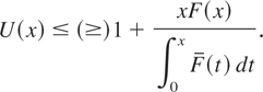
Provided that F has a finite first moment μ, the above inequality can be expressed as

Moreover, complementary bounds if u is increasing (decreasing) are given by

Proof: First we express (8) in terms of the renewal density. Since convolution is commutative between positive (possibly infinite) measures, we get

Assume now that u(x) is decreasing. Using Lemma 3.1, we then obtain that

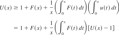
and the lower bound in (17) follows by solving for U(x).

For the upper bound in (19), note that (14) can be written as

Since u is decreasing and for a fixed x, F_e(x − t) is an increasing function of t, again using Lemma 3.1, we derive that

from which

Multiplying both sides by x gives

which, on replacing

and F_e(x) by 1 − F_e(x), reduces to

It is readily checked that the last inequality is the same as the upper bound in (19).

The proof of the complementary bounds in (17) and (19) for the case where u is increasing is similar. Finally, to show that the lower (upper) bound in (17) is the same as the corresponding bound in (18) when μ is finite, note that

and this concludes the proof. █

It is worth noting that for (17) to hold, we do not require the existence of any moments for F.

As already mentioned, if F is DFR, then the density u is decreasing and therefore the bound in (17) or (18) can be used. Since F will also belong to the NWUE class, the lower bound (3) is also applicable. In this case, the lower bounds provided by Theorem 3.2 are preferable over (3), as the next proposition indicates.

Proposition 3.3: If F is DFR, then the lower bound in Theorem 3.2 is sharper than the corresponding bound in (3) for all x ≥ 0.

Proof: For the result to hold, we require that F(x) − F_e(x) ≤ 0 for all x ≥ 0, which is the same as

However, this is obviously true; F being DFR implies that it is also NWUE. █

Assume now that F has a density f and let

be the associated renewal density. Here * denotes the usual convolution between integrable functions, defined by

, and f*^k is the kth convolution power of f.

If the distribution F is IMRL, it follows from the results of Brown [3] that there exists a version of the renewal density such that u(x) ≥ μ⁻¹ for x ≥ 0. Using this inequality on the right-hand side of the renewal equation

we obtain

and inserting this bound again into (21) yields

By induction, we get that for all m ≥ 1, the following inequality holds:

This gives a new bound for U via the relation

; more explicitly,

In view of the above-mentioned inequality, it is clear that

One possible use of this bound is the following. A very simple and commonly used approximation for U is based on truncating the series of convolution powers of F, so that

for some positive integer m. The bound above thus yields a lower bound for the truncation error of that approximation.

Finally, we mention that if F is DFR, then it is also concave (see, e.g., Sengupta and Nanda [16]), so that, in particular, it possesses a decreasing density, f (x). Thus, we have from (21),

and applying Lemma 3.1, we derive that

Solving this for U, we obtain the following lower bound:

4. BOUNDS UNDER AGING PROPERTIES FOR THE INTERARRIVAL TIMES

In this section we obtain refined bounds under various additional assumptions on the distribution F, which represents the interarrival time between renewals. More specifically, we consider the case where F belongs to an aging class of distributions, such as those mentioned in Section 1. Our first result concerns the IFR class of distributions.

Proposition 4.1: Let F be an IFR life distribution with finite mean μ and variance σ². Then for the renewal function associated with F, we have the lower bound

Proof: Inserting Brown's result (5) into (8) we get, by virtue of (11),

and the result follows immediately. █

Note that the new bound is better than that in (5) for all x such that

which is the same as m(x) ≥ σ²/μ. Since m(0) = μ > σ²/μ for any IFR distribution with finite mean, the previous condition is true at least in an interval [0,b) with 0 < b ≤ ∞. Further, when F is IFR with a finite mean, it is also DMRL, so that m(x) is decreasing. Thus, b = ∞ for all IFR distributions whose MRL function has a limit greater than or equal to σ²/μ (i.e., lim_x→∞ m(x) ≥ σ²/μ).

As an illustration, consider the case where F is a Gamma distribution with shape parameter α > 1 and scale parameter λ. Then it holds that

whereas for the MRL function m(x), we have

Thus, in this case, the lower bound for U(x) in Proposition 4.1 is an improvement over that in (5) for all x ≥ 0.

This is illustrated further in the following example where the two bounds in (5) and (22) are also compared with the lower bound given in Theorem 3.2. Note first that the lower bounds for U(x) from (19) apply when the renewal density u is increasing, and the lower bounds from (5) and Proposition 4.1 can be used when the underlying distribution F is IFR. Since, in general, F is IFR does not imply that u is increasing, we use a well-known example of a Gamma distribution with shape parameter greater than one (so that it is IFR) for which the renewal density is known to be increasing. This has the additional advantage that the renewal function can be found explicitly, so that the absolute as well as the relative performance of the various bounds can be assessed.

Example 4: Consider the IFR Gamma density f (x) = xe^−x, with associated renewal density

Brown's [4] bound for U(x) (cf. (5)) is, in this case,

whereas the lower bound from Proposition 4.1 takes the form

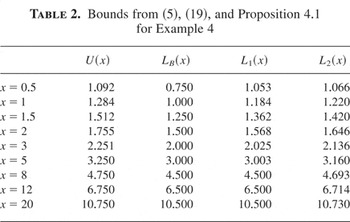
Call L_B(x) and L₁(x) the bounds from (5) and Proposition 4.1, respectively, and let L₂(x) be the lower bound for the renewal function from (19). Table 2 presents these bounds, as well as the true values for U(x), for various choices of x.

Bounds from (5), (19), and Proposition 4.1 for Example 4

As expected from the above expressions, L₁ is uniformly better than L_B; however, the improvement becomes negligible for large values of x. On the other hand, L₂ is much better than L_B for all values of x, and its relative performance over L₁ increases as x gets larger; we mention in particular, that, in contrast with the other two bounds, L₂ seems to possess the correct asymptotic behavior.

The last remark can be made rigorous; a standard result in renewal theory (see, e.g. [10]) is that

whereas a simple application of l'Hospital's rule in (19) yields

Note that this is valid for any distribution where the associated renewal density is increasing. It is worth noting that the correct asymptotic behavior of L₂ is also useful in the DFR case, when u is decreasing and L₂ is used as an upper bound.

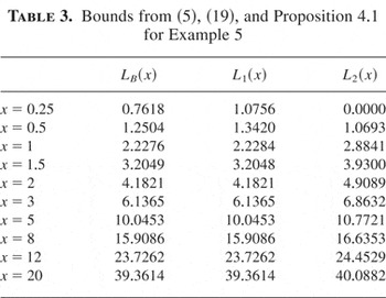
Example 5: Consider now the case where the interarrival distribution F in a renewal process has a Weibull density

so that F is again IFR. It is easy to see that in this case, lim_x→∞ m(x) = 0 and

Let L_B(x), L₁(x), and L₂(x) be the bounds from (5), Proposition 4.1, and (19) respectively. Table 3 presents these bounds for various choices of x. Compared with Table 2, we see that now L₂(x) is not uniformly superior to the other two bounds, as it performs poorly for very small values of x. For such values, L₁(x) improves significantly over L_B(x) and, as expected, when x becomes larger, the difference between these two values is negligible. For x ≥ 1, the bound from (19) exceeds the other two bounds by a steady amount of approximately 0.72.

Bounds from (5), (19), and Proposition 4.1 for Example 5

The rest of this section deals with upper and lower bounds for IMRL distributions. First, we recall that if F is IMRL, then H(x) = U(x) − x/μ is increasing (see, e.g., [3]). Then (6) gives

and for all x such that F(x) < 1, the next bound results for U(x):

Another upper bound is obtained by inserting Brown's bound (4) into (8); this gives

Observe that this is a refinement of (4) for all x such that

A lower bound for U in the IMRL case can also be obtained using the next simple result, which is easily verified. Let F_e⁽²⁾ be the equilibrium distribution corresponding to F_e. Then for x ≥ 0, the following identity holds:

Put now H₀(x) = H(x) − 1. Then from Brown [3], we have that H₀(x) is nonnegative and increasing. Thus, we can write

and since the left-hand side above is nonnegative, so is the right; therefore, we get H(x) ≥ (μ₂ /2μ²)F_e⁽²⁾(x) + F_e(x). This implies the following lower bound for U:

This is the same as Brown [3], on noting that Brown [3] allows F to have an atom at zero, which we have excluded here only for convenience.

Observe that from (23) and (25) we derive the following two-sided bound for U(x):

Next, since the IMRL class is a subfamily of the NWUE class, one might wonder whether the lower bound in (25) is a refinement over the corresponding bound for U in Corollary 2.3, and it is interesting to note that this is not true. In fact, for (25) to be an improvement over the lower bound given in (16), we need that

Using, for example, a Pareto distribution, one verifies easily that the last inequality is valid only for some x.

5. LOWER BOUNDS FOR TAILS OF COMPOUND GEOMETRIC DISTRIBUTIONS

Let X₁,X₂,…, be i.i.d. variables with cumulative distribution function F and let N be a geometric random variable (r.v.) such that P(N = n) = (1 − φ)φⁿ,n = 0,1,2,…,0 < φ < 1. Then the tail of the distribution for the random sum

is given by

Assume now that {N(x),x ≥ 0} is a renewal process with interarrival distribution F; Lin [11] proved the following relation between N(x) and the compound geometric tail in (26):

(see also Cai and Garrido [5]). Applying Jensen's inequality, we deduce that (see [15])

or, equivalently, solving for U(x),

Thus, bounds for U(x) can be used to deduce bounds for ψ(x) and vice versa. For instance, a bound for ψ is obtained immediately from Lorden's bound, U(x) ≤ x/μ + μ₂ /μ², and (27); namely

or

Further, using the bound U₁(x) (cf. Theorem 2.1) rather than Lorden's gives a different bound for ψ(x), which has the advantage that it is exact for x = 0 and it is better than the above bound for small values of x. Following the discussion after Theorem 2.1, we note in particular that the bound ψ(x) ≥ φ^U₁(x) is uniformly better than the bound in the last displayed expression if the underlying distribution F is NBUE.

6. CONCLUDING REMARKS

Interest in bounds for the renewal function exists also in the more general case where F is not concentrated on the nonnegative half-axis, so that it represents the step distribution of a random walk and U(x) denotes the expected number of visits in the interval (−∞,x] (see [10] for further details on this). An advantage of the method presented here is that it can be applied, without extra effort, for the case where F does not vanish on the negative half-axis. The passage from the one-sided case to the more general two-sided case is provided by the renewal equation

which should be used instead of (8). The analog of Lorden's bound for this more general case is given in [9], and concerning the performance of the bound, similar remarks apply to those for the one-sided case.

Finally, as mentioned after Theorem 2.1, the approach taken to prove that theorem can be used recursively. Thus, if one inserts the bound U₁(x) into the renewal equation (8), one obtains the bound

and, continuing in this way, we obtain after k successive iterations that

Letting k → ∞ yields the bound

which, in view of (14), shows that this procedure converges iteratively to the right solution for U(x).