A distributed force element method with matching of fundamental solutions

Zhiteng Zhou; Yi Liu; Zhenyu Zang; Zenghui Zhu; Hongping Wang; Shizhao Wang

doi:10.1017/jfm.2026.11373

A distributed force element method with matching of fundamental solutions

Published online by Cambridge University Press: 06 April 2026

and

Zhiteng Zhou: Affiliation:
State Key Laboratory of Nonlinear Mechanics, Institute of Mechanics, Chinese Academy of Sciences, Beijing, 100190, PR ChinaSchool of Engineering Sciences, University of Chinese Academy of Sciences, Beijing, 100049, PR China
Yi Liu: Affiliation:
State Key Laboratory of Nonlinear Mechanics, Institute of Mechanics, Chinese Academy of Sciences, Beijing, 100190, PR ChinaSchool of Engineering Sciences, University of Chinese Academy of Sciences, Beijing, 100049, PR China
Zhenyu Zang: Affiliation:
State Key Laboratory of Nonlinear Mechanics, Institute of Mechanics, Chinese Academy of Sciences, Beijing, 100190, PR ChinaSchool of Engineering Sciences, University of Chinese Academy of Sciences, Beijing, 100049, PR China
Zenghui Zhu: Affiliation:
State Key Laboratory of Nonlinear Mechanics, Institute of Mechanics, Chinese Academy of Sciences, Beijing, 100190, PR ChinaSchool of Engineering Sciences, University of Chinese Academy of Sciences, Beijing, 100049, PR China
Hongping Wang: Affiliation:
State Key Laboratory of Nonlinear Mechanics, Institute of Mechanics, Chinese Academy of Sciences, Beijing, 100190, PR ChinaSchool of Engineering Sciences, University of Chinese Academy of Sciences, Beijing, 100049, PR China
Shizhao Wang*: Affiliation:
State Key Laboratory of Nonlinear Mechanics, Institute of Mechanics, Chinese Academy of Sciences, Beijing, 100190, PR ChinaSchool of Engineering Sciences, University of Chinese Academy of Sciences, Beijing, 100049, PR China
*: Corresponding author: Shizhao Wang, wangsz@lnm.imech.ac.cn

Article contents

Abstract
Introduction
Pressure decomposition with fundamental solution
Results and discussion
Conclusion
Funding
Declaration of interests
References

Rights & Permissions

Abstract

Quantifying the contribution of vortex structures to wall forces is essential for identifying the primary sources of forces. The traditional force-element method focuses on the contribution of flow structures to the resultant force. However, the contribution of flow structures to the distributed force cannot be identified. This work proposes a distributed force element method to address this issue. Inspired by the framework of matched asymptotic expansions, the method resolves the surface pressure by matching the fundamental solutions of the outer wave and inner flow regions. The pressure is thus decomposed into contributions from a convective acceleration term, a boundary acceleration term and a boundary vorticity term. The method is implemented by solving the resulting linear system with singular value decomposition. The volume source is further decomposed into direct radiation and boundary scattering components. It is found that compared with the direct radiation component, the boundary scatter component decays fast in the wake. Consequently, the direct radiation component is dominant in the far wake. A finite-domain pressure correction is proposed based on the direct radiation component. The distributed force element method is validated using several benchmark cases: two-dimensional configurations including laminar flow around stationary and oscillating circular cylinders; three-dimensional cases comprising laminar flow past a sphere, subcritical flow past a sphere and laminar flow over an inclined spheroid. The results suggest that the proposed distributed force element method enables the precise quantification of how flow structures in the wake and around the bluff bodies contribute to the surface pressure.

JFM classification

Vortex Flows: Vortex dynamics

Information

Type: JFM Papers
Information: Journal of Fluid Mechanics , Volume 1032 , 10 April 2026, A56
DOI: https://doi.org/10.1017/jfm.2026.11373 [Opens in a new window]
Copyright: © The Author(s), 2026. Published by Cambridge University Press

1. Introduction

Understanding the physical origin of the hydrodynamic forces is one of the fundamental questions in fluid dynamics (Anderson Reference Anderson2011). It is directly relevant to diverse applications such as drag reduction (Russo et al. Reference Russo, Saetta, Tognaccini, Dacome and Demasi2021), sound source identification (Ji et al. Reference Ji, Jin, Huang, Wang, Ravi, Young, Lai and Tian2024) and the design of flow control strategies (Lu & Chang Reference Lu and Chang2025). Progress in these areas benefits from the ability to extract quantitative relationships between coherent flow structures and the resulting hydrodynamic forces from experimental or simulation data (Chang, Yang & Chu Reference Chang, Yang and Chu2008; Menon & Mittal Reference Menon and Mittal2021b ; Prakhar, Seo & Mittal Reference Prakhar, Seo and Mittal2025). This work proposes a new diagnostic method to spatially resolve how such flow structures contribute to the surface load distribution on the solid body.

Different methods have been developed to quantify the relationship between vortex structures and resultant forces. One approach uses impulse theory to link bulk flow features to resultant force, which is called the vorticity-moment method (Wu, Liu & Liu Reference Xu, Tian, Young and Lai2018). The vorticity-moment method traces its origins to foundational work in the early 20th century. Burgers (Reference Burgers1921) pioneered the concept by linking aerodynamic forces to the time rate of change of fluid impulse, proposing that vorticity generation and diffusion at the body surface govern resistance. This idea remained dormant until Wu (Reference Wu1981) and Lighthill (Reference Lighthill1986) revitalized and systematized the theory, establishing its modern framework for incompressible flows. They demonstrated that the resultant force on a body in unbounded flow could be expressed through a global integral of vorticity moments, bypassing direct pressure calculations. By using derivative-moment transformations, Wu, Pan & Lu (Reference Wu, Pan and Lu2005) proposed a formula for calculating the resultant force that relies solely on the boundary integrals over a control surface enclosing the solid body. The theory gained traction in biological propulsion studies, where discrete vortex structures dominate unsteady flows. Li & Lu (Reference Li and Lu2012) proposed a finite-domain impulse formulation and found that the resultant force on a flapping plate is determined solely by the two wake vortices that remain connected to the body. Kang et al. (Reference Kang, Liu, Su and Wu2018) later improved the theory by developing a minimum-domain approach, showing that forces could be determined using only the vorticity attached to or near the body, dramatically simplifying applications to complex wake interactions. The Galilean-invariance of different methods is discussed by Gao & Wu (Reference Gao and Wu2019). Recent applications by Liu, Zhu & Wu (Reference Liu, Zhu and Wu2015) bridged classical linear models with viscous flows, revealing how finite Reynolds number effects alter vortex shedding patterns.

Another approach relies on projecting the Navier–Stokes (NS) equations to an irrotational space to decompose the flow fields into different components, known as the force-element theory. The force-element theory decouples pressure from vortex structures (Quartapelle & Napolitano Reference Quartapelle and Napolitano1983), enabling direct calculation of a resultant force via vorticity (Chang Reference Chang1992; Chang et al. Reference Chang, Yang and Chu2008). The force-element theory originated in the early 1980s from the work of Quartapelle & Napolitano (Reference Quartapelle and Napolitano1983), who introduced auxiliary divergence-free vector fields to reformulate the pressure integral into volume integrals of acceleration and vorticity terms. Chang (Reference Chang1992) further refined the theory by introducing potential flow solutions around solid boundaries to account for their geometric role. Consequently, the forces acting on a bluff body can be decomposed into inertial (added-mass), vortical (Lamb vector) and viscous components, which enables a clear physical interpretation. Howe (Reference Howe1995) connected the theory to vortex–sound interactions by employing potential functions that are tied to body geometry, thereby unifying the mechanisms of force and sound generation. Hsieh et al. (Reference Hsieh, Kung, Chu and Chang2009) extended the application of this theory to biological locomotion, showcasing its ability to analyse unsteady flows by identifying the dominant force contributors. Recently, Gao, Xie & Lu (Reference Gao, Xie and Lu2025) proposed the weighted integral method. By introducing a weight function in the form of a second-order tensor, the weighted integral method provides a unified framework that enhances both the flexibility and accuracy of force and moment estimations.

Traditional potential-based methods, which rely on Gauss’s theorem, primarily resolve the resultant force rather than surface pressure, inherently limiting their ability to connect flow structures to distributed surface forces. Although the work of Gao et al. (Reference Gao, Xie and Lu2025), through a clever selection of weight function, offers an approach to analyse the source of surface pressure distribution on a two-dimensional (2-D) cylinder, a general method for identifying the origin of surface force distribution on arbitrary geometries is still lacking. This work proposes a distributed force element method that enables the spatial decomposition of surface pressure into physically interpretable source components for flows over general body shapes. A finite-domain correction is proposed to significantly reduce computational and storage demands. In implementation, inspired by the framework of matched asymptotic expansions (Kambe Reference Kambe1986; Kambe, Minota & Takaoka Reference Kambe, Minota and Takaoka1993), the distributed force element method employs superposition of fundamental solutions – a technique widely used in aeroacoustics (Lee et al. Reference Lee, Brentner and Morris2010, Reference Lee, Brentner and Morris2011; Lee Reference Lee2017) – to quantify contributions from flow structures at different locations. A robust singular value decomposition (SVD) algorithm is integrated to enhance numerical efficiency and stability.

The proposed distributed force element method functions as a postprocessing tool, starting from a complete NS solution that provides the baseline flow fields. For each point in the flow domain, the method computes the contribution of its corresponding source to the surface pressure by matching the inner flow field with a superposition of fundamental solutions (free-space Green’s functions) corresponding to virtual source points inside the solid body. The unknown strengths of these virtual sources are obtained by solving a linear system derived from the Neumann boundary condition. A key numerical advantage arises because, for flow around a stationary body, the coefficient matrices of these linear systems are independent of both the source locations and time. Consequently, their SVD needs to be computed only once, transforming subsequent solutions into efficient vector multiplications and additions, which significantly reduces the computational cost during repeated evaluations. However, for bodies in motion or with deforming boundaries, the coefficient matrices become time-dependent. In such cases, the matrix system must be recomputed at each time step, introducing additional computational overhead.

The remainder of this paper is organized as follows. Section 2 details the distributed force element method. Section 3 provides validations of the proposed method using both 2-D and three-dimensional (3-D) flows over solid bodies. Finally, the key findings and conclusions are summarized in § 4.

2. Pressure decomposition with fundamental solution

2.1. Partitioning of pressure fields

According to the NS equations for compressible flows, the governing equation of pressure $p$ can be written as

(2.1)

\begin{equation} \frac {1}{c_0^2} \frac {\partial ^2 p}{\partial t^2}-\Delta p=\boldsymbol{\nabla }\boldsymbol{\nabla }: \boldsymbol{T}, \end{equation}

where

(2.2)

\begin{equation} \boldsymbol{T}=\rho \boldsymbol{u} \boldsymbol{u}+ \big [(p-p_0)-c_0^2 (\rho -\rho _0)\big ] \boldsymbol{I}-\boldsymbol{\tau }, \end{equation}

under the homentropic assumption (Lighthill Reference Lighthill1952; Glegg & Devenport Reference Glegg and Devenport2017). Here, $\rho$ denotes density; $c_0$ , $p_0$ and $\rho _0$ are the speed of sound, pressure and density in the ambient flow; $\boldsymbol {u}$ represents fluid velocity; $\boldsymbol{I}$ is the unit tensor; $\boldsymbol{\tau }$ represents the viscous stress tensor. The Neumann condition at the solid boundary is required to specify the pressure uniquely. By projecting the NS equations to the norm $\boldsymbol {n}$ of the solid boundary, the Neumann condition can be obtained as

(2.3)

\begin{equation} \frac {{\partial p}}{{\partial n}} = \left ( { - \mu \boldsymbol{\nabla }\times {\boldsymbol{\omega }}} \right ) \boldsymbol{\cdot }{\boldsymbol {n}} - \rho _0 \frac {{{\textrm D}{\boldsymbol {u}}}}{{{\textrm D}t}} \boldsymbol{\cdot }{\boldsymbol {n}}, \end{equation}

where the first term on the right-hand side $ - \mu \boldsymbol{\nabla }\times {\boldsymbol{\omega }}$ denotes the effects of vorticity $\boldsymbol{\omega }$ and the second term $- \rho _0 ({{{\textrm D}{\boldsymbol {u}}}}/{{{\textrm D}t}}) \boldsymbol{\cdot }{\boldsymbol {n}}$ denotes the effects of acceleration of the solid boundary.

Figure 1.

Schematics of the spatial partitioning based on the dominant mechanism of pressure.

Kambe et al. (Reference Kambe, Minota and Takaoka1993) divided the pressure into inner flow region and outer wave region in low Mach number and relatively high Reynolds number flows for predicting far-field sound in free space. The Mach number is defined as $M$ and the Reynolds number ${\textit{Re}}$ hereinafter. As is shown the figure 1, the vorticity in the inner flow region is characterized by the space and velocity scales $l_v$ and $u_v$ . The corresponding time scale can be defined as $\tau _v = l_v / u_v$ . The pressure perturbation in the far field is characterized by the wavelength scale $\lambda = l_{v/M}$ , which is much larger than $l_v$ at low Mach numbers. In the outer wave region away from the source, the adiabatic relation is approximately satisfied and the viscosity effect can be neglected according to the estimation of Kambe et al. (Reference Kambe, Minota and Takaoka1993),

(2.4)

\begin{equation} \frac {{\left | {\boldsymbol{\nabla }\boldsymbol{\cdot }{\boldsymbol{\tau }}} \right |}}{{\left | {{\rho _0}\dfrac {{\partial {\boldsymbol {u}}}}{{\partial t}}} \right |}} = O\left ( {\frac {{\mu {\lambda ^{ - 2}}}}{{{\rho _0}{\tau _v ^{ - 1}}}}} \right ) = O \big( {{{{\mathop {Re}\nolimits } }^{ - 1}}{M^2}} \big). \end{equation}

Therefore, the source on the right-hand side of (2.1) is negligible and the pressure perturbation in the outer wave region is governed by the acoustic wave propagation as follows:

(2.5)

\begin{equation} \frac {1}{c_0^2} \frac {\partial ^2 p}{\partial t^2}-\Delta p=0. \end{equation}

In the inner flow region near the source, the pressure is governed by vortex dynamics. According to the work of Kambe et al. (Reference Kambe, Minota and Takaoka1993), we have

(2.6)

\begin{equation} \frac {\partial ^2 p}{c^2 \partial t^2} / \Delta p = O(M^2). \end{equation}

Therefore, $({1}/{{c_0^2}})({{{\partial ^2}p}}/{{\partial {t^2}}})$ can be neglected on the left-hand side of (2.1) in low Mach number flows. Meanwhile, the right-hand side of (2.1) can be reduced to $\rho _0 \boldsymbol{\nabla }\boldsymbol{\cdot }(\boldsymbol{{\boldsymbol {u}}} \boldsymbol{\cdot }\boldsymbol{\nabla }\boldsymbol{{\boldsymbol {u}}})$ with the adiabatic relation and the assumption of a relatively high Reynolds number. Therefore, (2.1) can be reduced to

(2.7)

\begin{equation} \Delta p = - \rho _0 \boldsymbol{\nabla }\boldsymbol{\cdot }(\boldsymbol{{\boldsymbol {u}}} \boldsymbol{\cdot }\boldsymbol{\nabla }\boldsymbol{{\boldsymbol {u}}}), \end{equation}

in the inner flow region. In incompressible flows, the right-hand side of (2.7) can alternatively be expressed in terms of the Q-invariant as $2\rho _0Q$ (Gao et al. Reference Gao, Zou, Shi and Wu2019).

2.2. Pressure decomposition in the inner flow region

According to the governing equation for pressure in the inner flow region, we decompose the pressure as follows:

(2.8)

\begin{equation} p = p_f + p_s, \end{equation}

where $p_f$ is the pressure from volume sources and satisfies

(2.9)

\begin{equation} \Delta p_f=- \rho _0 \boldsymbol{\nabla }\boldsymbol{\cdot }(\boldsymbol{{\boldsymbol {u}}} \boldsymbol{\cdot }\boldsymbol{\nabla }\boldsymbol{{\boldsymbol {u}}}), \end{equation}

in the fluid and

(2.10)

\begin{equation} \frac {{\partial p_f}}{{\partial n}} = 0, \end{equation}

on the solid boundary, while $p_s$ is the pressure from boundary sources and satisfies

(2.11)

\begin{equation} \Delta p_s=0, \end{equation}

in the fluid and

(2.12)

\begin{align} \frac {{\partial {p_s}}}{{\partial n}} = \left ( { - \mu \boldsymbol{\nabla }\times {\boldsymbol{\omega }}} \right ) \boldsymbol{\cdot }{\boldsymbol {n}} - {\rho _0}\frac {{{\textrm D}{\boldsymbol {u}}}}{{{\textrm D}t}} \boldsymbol{\cdot }{\boldsymbol {n}},\\[-15pt]\nonumber \end{align}

on the solid boundary. Inspired by the work of Curle (Reference Curle1955), Chang (Reference Chang1992) and Chang et al. (Reference Chang, Yang and Chu2008), we define Green’s functions $G_f$ and $G_s$ as follows:

(2.13)

\begin{equation} \begin{aligned} {\Delta}{G_f} &= \delta ({\boldsymbol {x}} - {\boldsymbol {y}}),\;{\textrm{ }}\partial {G_f}/\partial n = 0, \\ {\Delta }{G_s} &= 0,\;{\textrm{ }}\partial {G_s}/\partial n = \delta ({\boldsymbol {x}_{\boldsymbol {s}}} - {\boldsymbol {y}_{\boldsymbol {s}}}). \end{aligned} \end{equation}

An equation to obtain $p_f$ can be formulated by multiplying (2.9) with the corresponding Green’s function $G_f$ and subtracting it from the $p_f$ times the $G_f$ Laplacian:

(2.14)

\begin{equation} {p_f}\Delta {G_f} - {G_f}\Delta {p_f} = {p_f}\delta ({\boldsymbol {x}} - {\boldsymbol {y}}) - {G_f}\left ( { - \left ( \rho _0 {\boldsymbol{\nabla }\boldsymbol{\cdot }({\boldsymbol {u}} \boldsymbol{\cdot }\boldsymbol{\nabla }{\boldsymbol {u}})} \right )} \right ). \end{equation}

Integrating (2.14) of both sides over space yields

(2.15)

\begin{equation} \begin{aligned} &\int _{{V_R}} \left (\boldsymbol{\nabla }\boldsymbol{\cdot }\left (G_f\boldsymbol{\nabla }(p_f)\right )-\boldsymbol{\nabla }\boldsymbol{\cdot }\left (p_f\boldsymbol{\nabla }(G_f)\right ) \right )\,\text{d}V =\\ &\int _{{V_R}} {{G_f}\left ( { - \left ( {\rho _0 \boldsymbol{\nabla }\boldsymbol{\cdot }({\boldsymbol {u}} \boldsymbol{\cdot }\boldsymbol{\nabla }{\boldsymbol {u}})} \right )} \right )}\,\text{d}V - \int _{{V_R}} {{p_f}\delta ({\boldsymbol {x}} - {\boldsymbol {y}})}\,\text{d}V. \end{aligned} \end{equation}

Transforming the volume integral in the (2.15) into a boundary integral leads to

(2.16)

\begin{equation} \kern-1pc \int _{{S}} \left ({p_f}(\boldsymbol{\nabla }{G_f})\boldsymbol{\cdot }{\boldsymbol {n}} - {G_f}(\boldsymbol{\nabla }{p_f})\boldsymbol{\cdot }{\boldsymbol {n}}\right )\,\text{d}S = \int _{{V_R}} \!{{G_f} ( { - ( {\rho _0 \boldsymbol{\nabla }\boldsymbol{\cdot }({\boldsymbol {u}} \boldsymbol{\cdot }\boldsymbol{\nabla }{\boldsymbol {u}})} )} )})\,\text{d}V - {p_f}. \end{equation}

Substitute the boundary conditions of $ p_f$ and $ G_f$ into the (2.16) and utilize the sifting property of the $\delta$ function, we obtain

(2.17)

\begin{equation} {p_f} = \underbrace {\int _{{V_R}} { - \left ( {\rho _0 \boldsymbol{\nabla }\boldsymbol{\cdot }({\boldsymbol {u}} \boldsymbol{\cdot }\boldsymbol{\nabla }{\boldsymbol {u}})} \right )} {G_f}\,\text{d}V}_{{\textrm{convective }\;\textrm {acceleration }}}. \end{equation}

Similarly, we can follow the steps from (2.14) to (2.16) to obtain the formula for $ p_s$ :

(2.18)

\begin{equation} \int _{{S}} \left ({p_s}(\boldsymbol{\nabla }{G_f})\boldsymbol{\cdot }{\boldsymbol {n}} - {G_f}(\boldsymbol{\nabla }{p_s})\boldsymbol{\cdot }{\boldsymbol {n}}\right )\,\text{d}S = 0. \end{equation}

Substituting the boundary conditions of $ p_s$ and $ G_s$ into the above equation and utilizing the sifting property of the $\delta$ function, we obtain

(2.19)

\begin{equation} {p_s} = \underbrace { - \int _S {\mu \left ( {\boldsymbol{\nabla }\times {\boldsymbol{\omega }}} \right )} \boldsymbol{\cdot }{\boldsymbol {n}}{G_s}\,\text{d}S}_{{\textrm{boundary}}\;{\textrm{voticity}}}\underbrace { - \int _S {\left ( {{\rho _0}\frac {{{\textrm D}{\boldsymbol {u}}}}{{{\textrm D}t}} \boldsymbol{\cdot }{\boldsymbol {n}}} \right )} {G_s}\,\text{d}S}_{{\textrm{boundary}}\;{\textrm{acceleration}}} \end{equation}

on the solid boundary. The pressure on the solid boundary can thus be obtained by summing (2.17) and (2.19) as

(2.20)

\begin{align} p = \underbrace {\int _{{V_R}} { - \left ( {{\rho _0}\boldsymbol{\nabla }\boldsymbol{\cdot }({\boldsymbol {u}} \boldsymbol{\cdot }\boldsymbol{\nabla }{\boldsymbol {u}})} \right )} {G_f}\,\text{d}V}_{{\textrm{convective}\;\textrm {acceleration}}}\underbrace { - \int _S {\mu \left ( {\boldsymbol{\nabla }\times {\boldsymbol{\omega }}} \right )} \boldsymbol{\cdot }{\boldsymbol {n}}{G_s}\,\text{d}S}_{{\textrm{boundary}}\;{\textrm{voticity}}}\underbrace { - \int _S {\left ( {{\rho _0}\frac {{{\textrm D}{\boldsymbol {u}}}}{{{\textrm D}t}} \boldsymbol{\cdot }{\boldsymbol {n}}} \right )} {G_s}\,\text{d}S}_{{\textrm{boundary}}\;{\textrm{acceleration}}}.\\[-22pt]\nonumber \end{align}

Notably in (2.20), the pressure on the solid boundary originates from convective acceleration of fluid elements, boundary vorticity and acceleration of the solid boundary. For convenience of expression, we refer to the source term of $ p_f$ in the flow field as the convective volume source and the source term of $ p_s$ on the solid boundary as the vorticity–acceleration boundary source. Here, the vorticity–acceleration boundary source can be further divided into the vorticity boundary source and the acceleration boundary source, representing the sources of boundary vorticity and boundary acceleration, respectively.

2.3. Reconstruction of Green’s function

The pressure decomposition in (2.20) requires Green’s functions $ G_f$ and $ G_s$ , which depend on the geometry of the solid boundary. For complex geometries, obtaining these functions analytically is intractable. Instead of seeking analytical expressions, we introduce a numerical method to reconstruct Green’s function. The basic idea is to approximate the pressure field by superimposing fundamental solutions (i.e. free-space Green’s functions) originating from a set of virtual source points $ \boldsymbol{y}_j$ placed inside the solid body. The strengths of these sources, $ S(\boldsymbol{y}_j)$ , are determined by enforcing the prescribed Neumann boundary conditions ((2.10) and (2.12)) at a finite number of collocation points on the actual solid boundary. This process can effectively construct a solution that satisfies the boundary conditions approximately. Similar methodology has been successfully applied to the problem of acoustic field reconstruction (Lee, Brentner & Morris Reference Lee, Brentner and Morris2010; Lee Reference Lee2017; Wang et al. Reference Wang, Rienstra, Bi and Koren2020). It should be noted that the fundamental solution employed in this work is of the simplest monopole type, which has been widely adopted in acoustic scattering problems (Lee Reference Lee2017). The application of the monopole-type fundamental solutions is subject to certain limitations, particularly in the presence of thin inclusions such as cracks or domains with twisting boundaries (Alves & Leitão Reference Alves and Leitão2006). Various approaches, focusing for instance on the selection of alternative fundamental solutions (Hou, Zhang & Angland Reference Hou, Zhang and Angland2014) or the regularization of the resulting coefficient matrix (Xu, Mao & Hu Reference Xu, Mao and Hu2019), have been proposed to address these issues. A detailed discussion of such improvements, however, lies outside the scope of the present work.

Based on the fundamental solutions, the outer field pressure can be expressed as follows:

(2.21)

\begin{equation} p\left ( {{\boldsymbol {x}},t} \right ) = \sum \limits _j {\int _{ - \infty }^\infty {} S({{\boldsymbol {y}}_j},t_1 )} {G_{\textit{out}}}({\boldsymbol {x}},{{\boldsymbol {y}}_j};t,t_1 )\textrm{d}t_1 , \end{equation}

where ${G_{\textit{out}}}({\boldsymbol {x}},{{\boldsymbol {y}}_j};t,t_1 )$ is the fundamental solution for the wave equation in outer wave region. The fundamental solution is given by

(2.22)

\begin{equation} G{_{\textit{out},3\textit{D}}}(\boldsymbol{x}, \boldsymbol{y}_j; t, t_1) = \frac {\delta \left ( t - t_1 - |\boldsymbol{x} - \boldsymbol{y}_j| / c_0 \right )}{4 \pi |\boldsymbol{x} - \boldsymbol{y}_j|}, \end{equation}

and

(2.23)

\begin{equation} G{_{\textit{out},2\textit{D}}}(\boldsymbol{x}, \boldsymbol{y}_j; t, t_1) = \frac {H \left ( t - t_1 - |\boldsymbol{x} - \boldsymbol{y}_j| / c_0 \right )} {2 \pi \sqrt {(t-t_1)^2 - |\boldsymbol{x} - \boldsymbol{y}_j|^2 / c_0^2}}, \end{equation}

for 3-D and 2-D problems, respectively. Here $\delta (\boldsymbol{\cdot })$ denotes the Dirac delta function and $H(\boldsymbol{\cdot })$ the Heaviside step function. Here, $\boldsymbol{x}$ and $t$ are the position and time at which the pressure is evaluated (the observer), whereas $\boldsymbol{y}$ and $t_1$ designate the position and time of the virtual source. Here ${S}({{\boldsymbol {y}}_j} ,t_1)$ is the strength of the jth virtual source. When the virtual sources are close to the observers, the fundamental solutions can be reduced to

(2.24)

\begin{equation} \begin{aligned} p ( {{\boldsymbol {x}},t} ) &= \sum \limits _j {S({{\boldsymbol {y}}_j},t)\frac {1}{{4\pi | {{\boldsymbol {x}} - {{\boldsymbol {y}}_j}} |}}} ,\\ p ( {{\boldsymbol {x}},t} ) &= \sum \limits _j {S({{\boldsymbol {y}}_j},t)\left ( { - \frac {{\ln ( {| {{\boldsymbol {x}} - {{\boldsymbol {y}}_j}} |} )}}{{2\pi }}} \right )} , \end{aligned} \end{equation}

for 3-D and 2-D problems. For the sake of brevity in notation, we denote the reduced fundamental solution as $G$ and omit the explicit time variable. Consequently, (2.24) can be rewritten as

(2.25)

\begin{equation} p\left ( {\boldsymbol {x}} \right ) = \sum \limits _j {S({{\boldsymbol {y}}_j})} {G}({\boldsymbol {x}},{{\boldsymbol {y}}_j}). \end{equation}

For a volume source $\delta (\boldsymbol {y}_{\boldsymbol {f}}-\boldsymbol {y}_{\boldsymbol {0}})$ in the fluid, the intensities of the virtual sources can be determined as follows by matching the norm pressure gradient on the solid boundary (2.10):

(2.26)

\begin{equation} \sum \limits _j {S({{\boldsymbol {y}}_j},{{\boldsymbol {y}}_0})\frac {{\partial G({\boldsymbol {x}},{{\boldsymbol {y}}_j})}}{{\partial {x_i}}}} {n_i} = - \frac {{\partial G({\boldsymbol {x}},{{\boldsymbol {y}}_0})}}{{\partial {x_i}}}{n_i}. \end{equation}

Then, the Green’s function $G_f$ can be obtained as

(2.27)

\begin{equation} {G_f}({\boldsymbol {x}},{{\boldsymbol {y}}_0}) = G({\boldsymbol {x}},{{\boldsymbol {y}}_0}) + \sum \limits _j {S({{\boldsymbol {y}}_j},{{\boldsymbol {y}}_0})} G({\boldsymbol {x}},{{\boldsymbol {y}}_j}). \end{equation}

The first term on the right-hand side represents the Green’s function in free space, which is independent of the geometry of the wall and is related only to the positions of the measurement point and the source. The second term on the right-hand side, in contrast, accounts for the influence of the solid boundary on the pressure propagation. For the convenience of expression, the second term $\sum \nolimits _j {S({{\boldsymbol {y}}_j},\boldsymbol {y})} {G}({\boldsymbol {x}},{{\boldsymbol {y}}_j})$ is defined as $G_1$ . Green’s function $G_f$ is thus $G_f=G+G_1$ . Following the work for diffraction problem in low-Mach-number compressible flows (Gloerfelt et al. Reference Gloerfelt, Pérot, Bailly and Juvé2005), $G$ can be regarded as Green’s function for direct radiation from a volume source and $G_1$ as Green’s function for effects of boundary scattering to pressure propagation. Accordingly, the pressure can be further decomposed as follows:

(2.28)

\begin{equation} \begin{aligned} p =& \underbrace {\int _{{V_R}} { - \left ( {\rho _0\boldsymbol{\nabla }\boldsymbol{\cdot }({\boldsymbol {u}} \boldsymbol{\cdot }\boldsymbol{\nabla }{\boldsymbol {u}})} \right )} G\,\text{d}V}_{{\textrm{direct}}\;{\textrm{radiation}}} + \underbrace {\int _{{V_R}} { - \left ( {\rho _0\boldsymbol{\nabla }\boldsymbol{\cdot }({\boldsymbol {u}} \boldsymbol{\cdot }\boldsymbol{\nabla }{\boldsymbol {u}})} \right )} {G_1}\,\text{d}V}_{{\textrm{boundary}}\;{\textrm{scattering}}}\\ &\underbrace { - \int _S {\mu \left ( {\boldsymbol{\nabla }\times {\boldsymbol{\omega }}} \right )} \boldsymbol{\cdot }{\boldsymbol {n}}{G_s}\,\text{d}S}_{{\textrm{boundary}}\;{\textrm{voticity}}}\underbrace { - \int _S {\left ( {{\rho _0}\frac {{{\textrm D}{\boldsymbol {u}}}}{{{\textrm D}t}} \boldsymbol{\cdot }{\boldsymbol {n}}} \right )} {G_s}\,\text{d}S}_{{\textrm{boundary}}\;{\textrm{acceleration}}}. \end{aligned} \end{equation}

The first and second terms in the first line on the right-hand side of (2.28) are denoted as $p_{\textit{fd}}$ and $p_{\textit{fs}}$ hereinafter. For a boundary source $\delta (\boldsymbol {y}_{\boldsymbol {s}}-\boldsymbol {y}_{\boldsymbol {0}})$ on the solid boundary, the intensities of the virtual sources can be determined as follows by using (2.12):

(2.29)

\begin{equation} \sum \limits _j {S({{\boldsymbol {y}}_j},{{\boldsymbol {y}}_0})\frac {{\partial G({\boldsymbol {x}},{{\boldsymbol {y}}_j})}}{{\partial {x_i}}}} {n_i} = \delta (\boldsymbol {y}_{\boldsymbol {s}}-\boldsymbol {y}_{\boldsymbol {0}}). \end{equation}

Then, the Green’s function $G_s$ can be obtained as

(2.30)

\begin{equation} G_s({\boldsymbol {x}},{{\boldsymbol {y}_{\boldsymbol {0}}}}) = \sum \limits _j {S({{\boldsymbol {y}}_j},\boldsymbol {y}_{\boldsymbol {0}})} {G}({\boldsymbol {x}},{{\boldsymbol {y}}_j}). \end{equation}

Equations (2.26) and (2.29) can be written in the matrix form as follows:

(2.31)

\begin{equation} \boldsymbol{b} = \boldsymbol{Aq}, \end{equation}

where the matrix $\boldsymbol{A}$ has elements $A_{mn} = {\partial G(\boldsymbol{x}_n, \boldsymbol{y}_m)}/{\partial x_i}$ at the $m$ th row and $n$ th column. Here $\boldsymbol{q}$ is a column vector, representing the unknown strengths for the virtual sources. The nth element in $\boldsymbol{b}$ is $ - ( {{\partial G({{\boldsymbol {x}}_n},{{\boldsymbol {y}}_0})}}/{{\partial {x_i}}}){n_i}$ for the volume source and $\delta (\boldsymbol {y}_{\boldsymbol {s}}-\boldsymbol {y}_{\boldsymbol {0}})$ for the boundary source. The matrix $\boldsymbol{A}$ might be a rectangular matrix since fewer virtual sources may be used than the collocation points. Therefore, the SVD can be employed to obtain the least-squares solution of the (2.31). By using the SVD, the solution of (2.31) is transformed into vector multiplication and addition as follows:

(2.32)

\begin{equation} {\boldsymbol {q}} \approx \sum \limits _{i = 1}^{{n_c}} {\frac {1}{{{s_i}}}{{\boldsymbol {v}}_i}{\boldsymbol {u}}_i^T\boldsymbol{b}}, \end{equation}

where $n_c$ is the number of selected modes, taken as the number of virtual sources in this work. Here $s_i$ denotes the $i$ th singular value of matrix $\boldsymbol{A}$ , while $\boldsymbol{v}_i$ and $\boldsymbol{u}_i$ represent the $i$ th right and left singular vectors, respectively.

3. Results and discussion

This section validates the pressure reconstructed by the proposed distributed force element method against results obtained by solving the NS equations. The study begins with a 2-D flow over a circular cylinder to examine the method’s sensitivity to its parameters and to simplify the contribution of far-field volume sources. It then proceeds to 3-D flow cases to diagnose the underlying physical mechanisms governing the surface pressure distribution and pressure drag.

Figure 2.

Schematics of (a) computational grid and (b) domain employed in the simulation of laminar flow over a circular cylinder.

3.1. Two-dimensional flows over a circular cylinder

3.1.1. Numerical methods and set-ups

The distributed force element method is first validated using a 2-D flow over a circular cylinder fixed in a uniform free stream flow. The flows over a rigid circular cylinder of diameter $D$ is immersed in a uniform free stream with speed $U$ , as depicted in figure 2. The origin of the coordinate system is located at the centre of the cylinder’s surface. The $y_1$ axis is aligned with the uniform free stream flow and the $y_2$ axis is perpendicular to the $y_1$ axis, defining the vertical direction. The flows around the circular cylinder are obtained by numerically solving using the NS equations,

(3.1)

\begin{equation} \begin{aligned} &\frac {{\partial \rho }}{{\partial t}} + \frac {\partial }{{\partial {y_i}}} ( {\rho {u_i}} ) = 0,\\ &\frac {{\partial ( {\rho {u_i}} )}}{{\partial t}} + \frac {{\partial ( {\rho {u_i}{u_j}} )}}{{\partial {y_j}}} + \frac {{\partial p}}{{\partial {y_i}}} = \frac {{\partial {\tau _{ij}}}}{{\partial {y_j}}},\\ &\frac {{\partial ( {\rho {e_t}} )}}{{\partial t}} + \frac {{\partial ( {\rho {u_i}{e_t}} )}}{{\partial {y_i}}} + \frac {{\partial ( {p{u_i}} )}}{{\partial {y_i}}} = \frac {{\partial ( {{u_i}{\tau _{ij}}} )}}{{\partial {y_i}}} - \frac {{\partial ( {{q_i}} )}}{{\partial {y_i}}}, \end{aligned} \end{equation}

where ${u}_{i}$ represents the component of the velocity field. Here $\rho ,p,T,{{e}_{t}}$ are the density, pressure, temperature and total energy, respectively. The viscous stress ${\tau }_{ij}$ and component of the heat flux vector $q_i$ are computed as

(3.2)

\begin{equation} {\tau _{ij}} = \mu \left ( {\frac {{\partial {u_i}}}{{\partial {y_j}}} + \frac {{\partial {u_j}}}{{\partial y_i}} - \frac {2}{3}\frac {{\partial {u_k}}}{{\partial {y_k}}}{\delta _{ij}}} \right ),\quad {q_i} = - \lambda \frac {{\partial T}}{{\partial {y_i}}}. \end{equation}

The subscripts in the above equation denote the components of each quantity, where Einstein’s index notation will be used. The molecular viscosity $\mu$ and thermal conductivity coefficient $\lambda$ are computed according to Sutherland’s law.

The numerical simulation of flow around a circular cylinder is conducted by using an in-house solver for NS equations. This solver employs a second-order Roe scheme for discretizing convective fluxes and a reconstructed central scheme for computing viscous fluxes. An implicit dual-time stepping method of second-order accuracy is utilized for time integration. Additionally, adaptive techniques such as local time-step adjustments and flux blending are incorporated to enhance the stability and convergence of the solution. Comprehensive details regarding the implementation and verification of this numerical approach have been previously documented in our studies (Liu et al. Reference Liu, Zhou, Zhu and Wang2021, Reference Liu, Wang, Wang and He2023).

The computational domain is defined as a circle with a radius $1342D$ , as shown in figure 2. A non-reflecting characteristic far-field boundary condition is applied at the outer boundary and the surfaces of the cylinder are modelled as no-slip, adiabatic walls. The computational grid is structured. The minimum grid spacing is approximately $5 \times 10^{-3}D$ resulting in a total number of approximately 264 471 cells. An implicit time-advancement scheme is used with a time step of $6 \times 10^{-3}D/U$ . The free stream flows are set to a Mach number of $M=0.03$ and a Reynolds number based on the cylinder diameter of ${\mathop {Re}\nolimits } = UD/\nu = 150$ , where $\nu$ is the kinematic viscosity.

To decompose the surface pressure, we set 200 collocation points uniformly distributed on the solid boundary. As shown in figure 3, the integration domain of the volume source is defined as a rectangular region enclosing the cylinder, expressed in coordinates as $[y_{\textit{left}}, y_{\textit{right}}] \times [y_{\textit{bottom}}, y_{\textit{top}}]$ . In this case, $y_{\textit{left}}$ , $y_{\textit{bottom}}$ and $y_{\textit{top}}$ are specified as $-2D$ , $-5D$ and $5D$ , respectively. The selection of the right-hand boundary’s position and the integration domain’s shape are discussed in Appendices A and B, respectively.

Figure 3.

Schematics of the laminar flows over a circular cylinder and set-up of the distributed force element method.

3.1.2. Effects of numerical set-up on the 2-D distributed force element method

In implementation, the proposed distributed force element method requires setting parameters such as the position and number of virtual sources. In this section, the flow over a circular cylinder is used as a benchmark to test the proposed distributed force element implementation, focusing on the position and number of virtual sources, as well as the mesh size for volume source integration. In the postprocessing step, the volume source data are first interpolated from the non-uniform CFD mesh onto a uniform grid before integration is performed. The mesh size here refers to the edge length of the uniform grid cells.

Figure 4.

Comparison of the results from CFD and the proposed distributed force element varying with (a) the number of virtual sources,(b) the position of virtual sources and (c) mesh size for integration of the convective acceleration term, panels (d)–(f) are the absolute errors corresponding to (a)–(c).

Figure 4 presents the computed instantaneous surface pressure distributions on the cylinder for different numbers and positions of virtual sources, as well as for varying mesh sizes used in the volume-source integration. Figure 4(a–c) compare the surface pressure reconstructed by the proposed distributed force element method with the CFD results, while figures 4(d) to 4(f) show the corresponding absolute errors. Here $y_{\textit{right}}$ is set to $30D$ . The number of virtual sources is set to approximately $ N_c/6$ , $ N_c/5$ , $ N_c/4$ , $ N_c/3$ and $ N_c/2$ , where $ N_c$ is the number of collocation points on the cylinder surface. The virtual sources are positioned along a circle at distances ranging from 0.05 $D$ to 0.4 $D$ from the cylinder centre. The mesh size for integration ranges from 0.05 $D$ to 0.01 $D$ . The detailed set-up of the cases is summarized in table 1. As observed in the figures, the results obtained from the distributed force element method remain consistent across different numbers of virtual sources and agree well with the reference CFD data. From figure 4(d), the overall trend and magnitude of the absolute error show little sensitivity to the number of virtual sources; however, increasing their count introduces oscillatory behaviour in the error. Regarding the placement of equivalent sources, figure 4(e) indicates that when the sources are positioned very close to the cylinder centre (within 0.1 $D$ ), the absolute error becomes larger and exhibits oscillations. Moving the sources farther from the centre stabilizes the error, suggesting that a highly clustered arrangement may lead to numerical instability in solving the system of equations for this case. With respect to the mesh size – where square cells are used for volume-source integration – the distribution of absolute error along the wall appears sensitive to this parameter.

Table 1.

Comparison of relative error for pressure computed by using the distributed force element method with different virtual sources’ numbers, positions and mesh size for integration.

To quantify the accuracy of the distributed force element methods, the relative error $\varepsilon$ is defined as follows:

(3.3)

\begin{equation} \varepsilon = \frac {{ \| {{p_{\textit{dfe}}} - {p_{\textit{cfd}}}} \|}}{{\| {{p_{\textit{cfd}}}} \|}}, \end{equation}

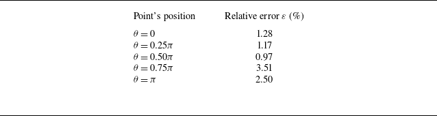
where $ {p_{\textit{dfe}}} \equiv {p_f} + {p_s}$ denotes the outcome from the distributed force element method, and $ {p_{\textit{cfd}}}$ represents the accurate result extracted from the computations. Table 1 reveals that the relative errors are all below 2 % for different number of equivalent sources. For the positions of virtual sources, the results deviate significantly from the direct numerical simulation (DNS) results only at $ R_s = 0.1D$ , while for other positions, the relative errors remain below 2 %. As for the integration mesh size, the maximum error is 2.9 % for the coarsest mesh of 0.05 $D$ , while errors for all other mesh sizes are below 2 %. These results demonstrate the reliability of the proposed distributed force element method in the current case. To balance computational cost and accuracy, the number of virtual sources used in the 2-D flow over a stationary circular cylinder is set to $ N_c/3$ , consistent with the recommendation by Dunn & Tinetti (Reference Dunn and Tinetti2004), the position of the virtual sources is set to 0.3 $D$ , and the mesh size for integration is set to 0.02 $D$ .

Figure 5 shows the decomposition of pressure at different locations on the surface of the circular cylinder. The solid dots denote directly sampled values from the simulated flow field, referred to as standard results hereinafter. The solid lines represent the results obtained using the proposed distributed force element method, (2.20), the dotted lines represent the contributions from the convective volume sources and the dashed lines represent the contributions from the vorticity–acceleration boundary sources. Here, $\theta =0$ indicates the rear stagnation point of the cylinder, and $\theta =\pi$ indicates the front stagnation point of the cylinder. It can be observed that the surface pressure on the circular cylinder predicted by the distributed force element method aligns closely with results directly extracted from the computation. As indicated in table 2, the relative errors at all measurement points on the wall remain below 5 %. Notably, the pressure at $\theta = 0.75\pi$ is the closest to zero among these points and, as expected, exhibits the largest relative error of 3.51 %. From the $\theta =0$ to $\theta =\pi$ , the pressure fluctuation increases first and then decreases from the rear stagnation point to the front stagnation point. This observation suggests that the pressure fluctuation along the streamwise direction is weaker than that along the vertical direction. Thus, the fluctuation of pressure drag is much smaller than that of pressure lift. The pressure fluctuation at different measurement points mainly comes from the convective volume source. For instance, for the point at $\theta =0.5\pi$ , the amplitude of the pressure fluctuation contributed by the boundary source is approximately ${1}/{8}$ of that contributed by the volume source. Furthermore, the direct radiation part of the convective volume source is closest to the pressure at each measurement point, except for the point at $\theta = \pi$ . At the measurement point where $\theta = \pi$ , the contribution of the direct radiation part of the volume source term is close to zero, which suggests that the direct radiation parts of the positive and negative volume sources cancel each other out near the stagnation point.

Table 2.

Comparison of relative error for pressure computed by using the distributed force element method on the circular cylinder’s surface.

Figure 5.

Comparison of the pressure computed by summing the contribution from convective volume source and vorticity–acceleration boundary sources and standard results at (a) $\theta =0$ , (b) $\theta =0.25\pi$ , (c) $\theta =0.5\pi$ , (d) $\theta =0.75\pi$ , (e) $\theta =\pi$ on the solid boundary.

3.1.3. Finite-domain pressure correction

As outlined in the literature (Gao et al. Reference Gao, Xie and Lu2025; Xie et al. Reference Xie, Liu, Zhou and Wang2026) and Appendix A, an accurate decomposition of distributed force requires integration of the volume source term $Q$ over a sufficiently large domain. This leads to significant computational and storage demands, especially for 3-D problems. Therefore, we seek a method capable of providing a correct decomposition of the distributed force using only flow field information within a limited region. To this end, we analysed the contribution of the volume sources in the wake to the distributed force.

Figure 6.

Comparison of the contribution from the direct radiation and boundary scattering component.

Figure 6 illustrates the comparison between the contributions of the volume sources’ direct radiation and the boundary scattering components to the surface pressure of the circular cylinder. The distribution of these two components is markedly different. The boundary scattering component is primarily concentrated near the cylinder and decays rapidly in the wake. In contrast, the direct radiation component is more uniformly distributed and extends further into the wake. Additionally, in regions of the wake that are far from the solid boundary, the distribution of direct radiation remains nearly constant regardless of the wall measurement point’s location and is significantly greater than the contribution from the boundary scattering component. This finding indicates that the differences in surface pressure measurements are primarily due to the flow near the cylinder surface. Since the resultant pressure force on the cylinder arises from the pressure difference across the cylinder surface, this finding also indicates that the lift and drag forces on the cylinder have a weak dependence on the far wake. Therefore, we propose to use pressure measurements at a single point on the wall as a reference. A finite-domain surface pressure correction can be given as follows:

(3.4)

\begin{equation} \begin{aligned} p &= \int _{{V_R}} { - \left ( {{\rho _0}\boldsymbol{\nabla }\boldsymbol{\cdot }({\boldsymbol {u}} \boldsymbol{\cdot }\boldsymbol{\nabla }{\boldsymbol {u}})} \right )} {G_f}\,\text{d}V - \int _S {\mu \left ( {\boldsymbol{\nabla }\times {\boldsymbol{\omega }}} \right )} \boldsymbol{\cdot }{\boldsymbol {n}}{G_s}\,\text{d}S - \int _S {\left ( {{\rho _0}\frac {{{\textrm D}{\boldsymbol {u}}}}{{{\textrm D}t}} \boldsymbol{\cdot }{\boldsymbol {n}}} \right )} {G_s}\,\text{d}S \nonumber\\ &\quad +\, {p_{{\textit{correct}}}}. \end{aligned} \end{equation}

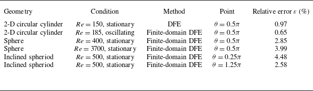
Here, $p_{\textit{correct}}(t)$ denotes the pressure correction term derived from measurements at a single point on the cylinder surface. This correction term $p_{\textit{correct}}(t)$ evolves over time yet remains invariant with respect to the specific location of the measurement points on the cylinder surface. A detailed discussion of (3.4) is provided in Appendix B. The application of this correction in a 2-D case (flow around an oscillating cylinder) is demonstrated in Appendix C. In the subsequent 3-D study of flow past a sphere, the same correction (3.4) is employed throughout. This correction is attributed primarily to the direct radiation component of the volume source and is, therefore, incorporated into the total contribution from the convective volume source in the subsequent analysis. Furthermore, Appendix D has been added to examine the applicability of the proposed distributed element method with pressure correction to other geometries, specifically the flow around an inclined spheroid.

3.2. Flows over a sphere

3.2.1. Numerical methods and set-ups

The simulations for the flow past a sphere employ the same governing equations, numerical methods and in-house solver as described for the 2-D stationary circular cylinder case. The computational domain is 3-D, encompassing a rigid sphere of diameter $D$ immersed in a uniform free stream with velocity $U$ , as shown in figure 7. The origin of the coordinate system is placed at the sphere’s centre.

Figure 7.

Schematics of (a) computational domain and (b) grid employed in the simulation of flow over a sphere.

A structured grid is employed to discretize the computational domain, which is defined as a rectangular region. The minimum grid spacing normal to the wall is approximately $6 \times 10^{-4}D$ , yielding a total of approximately $27\times10^6$ cells. A non-reflecting characteristic far-field condition is applied at the domain boundaries. The sphere surface is modelled as a no-slip, adiabatic wall. The free stream conditions are set to a Mach number of $M=0.1$ and Reynolds numbers based on the sphere diameter of $Re=UD/\nu$ = 400 (laminar flow) (Feng & Michaelides Reference Feng and Michaelides2001) and 3700 (subcritical flow) (Rodriguez et al. Reference Rodriguez, Borell, Lehmkuhl, Segarra and Oliva2011). The laminar flow is simulated by directly solving the governing equations, while the subcritical flow is solved by using the large-eddy simulation (LES). The eddy viscosity model proposed by Vreman (Reference Vreman2004) is used. The time steps for the implicit time-advancement scheme are both set to $1 \times 10^{-2}D/U$ for the two simulations.

3.2.2. Effects of numerical set-up on the 3-D distributed force element method

To validate the proposed distributed force element method in 3-D conditions, we simulate a laminar flow over a sphere fixed in a uniform free stream.

The virtual sources are positioned at $0.3D$ from the sphere centre. The integration domain of the volume source is defined as a rectangular region enclosing the sphere. In this case, the integration region of volume source along the $y_2$ and $y_3$ direction is specified as $-D$ to $D$ . The pressure correction of (3.4) is used as the volume source region is truncated at $y_{\textit{right}}=2D$ .

Figure 8.

Comparison of the results from computational fluid dynamics (CFD) and the proposed distributed force element method varying with (a) the number of virtual sources and (b) the position of virtual sources; panels (c) and (d) are the absolute errors corresponding to (a) and (b).

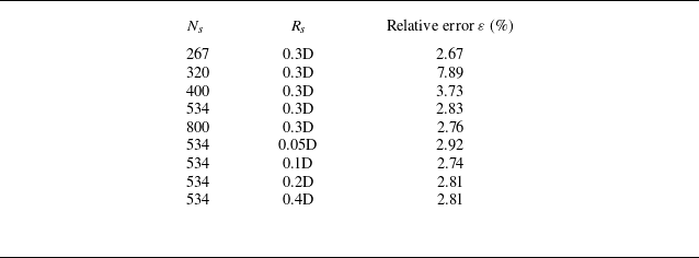
Figures 8(a) and 8(b) display the computed instantaneous surface pressure distributions on the sphere at $y_3 = 0.0D$ for different numbers and positions of virtual sources. The corresponding absolute error are shown in figures 8(c) and 8(d). The number of virtual sources is set to approximately $ N_c/6$ , $ N_c/5$ , $ N_c/4$ , $ N_c/3$ and $ N_c/2$ , where $ N_c$ is the number of collocation points on the sphere. The virtual sources are positioned on a sphere at distances ranging from 0.05D to 0.4D from the sphere centre. The detailed set-up of the cases is summarized in table 3. As shown in the figures, the distributed force element results are consistent across different numbers of virtual sources and align well with the accurate results. Table 3 indicates that the relative errors remain below 3 % across most tested numbers of virtual sources, except for the case with $N_s=320$ . Regarding the position of virtual sources, the relative errors are also below 3 %, with the maximum value observed being 2.92 %. For the absolute error, as illustrated in figures 8(c) and 8(d), the overall distribution shows lower values near the rear stagnation point (around $\theta = 0$ ) and higher values near the front stagnation point ( $\theta = \pi$ ). This pattern arises because the current finite-domain correction is designed to match the pressure at the rear stagnation point; consequently, the error tends to increase with distance from this reference location. These observations demonstrate the reliability of the proposed distributed force element method in the current case. To balance computational cost and accuracy, the number of virtual sources used in the 3-D case in this work is set to $ N_c/3$ and the position of the virtual sources is set to 0.3D.

Table 3.

Comparison of relative error for pressure computed by using the distributed force element method with different virtual sources’ numbers and positions.

3.2.3. Instantaneous distributed force decomposition for laminar flow over a sphere

Figure 9 shows the instantaneous flow field around a sphere. The vortex tubes are depicted by the isosurface of $ QD^2/U^2 = 0.001$ , with the background coloured according to the non-dimensional convective volume source $ ( {\boldsymbol{\nabla }\boldsymbol{\cdot }({\boldsymbol {u}} \boldsymbol{\cdot }\boldsymbol{\nabla }{\boldsymbol {u}})} ) D^2/U^2$ . Additionally, the distributions of $ ( {\boldsymbol{\nabla }\boldsymbol{\cdot }({\boldsymbol {u}} \boldsymbol{\cdot }\boldsymbol{\nabla }{\boldsymbol {u}})} ) D^2/U^2$ on four cross-sections perpendicular to the streamwise direction (i.e. the $y_2-y_3$ planes) are presented. These cross-sections, labelled A, B, C and D, correspond to streamwise positions $y_1/D$ = −0.5, 0, 1.0 and 2.0, respectively. As shown in the figure, the volume source is primarily concentrated near the sphere and around the vortex tubes in the wake. Positive volume sources appear near the stagnation point, while the shear layer is dominated by negative sources. In the near wake, low-intensity sources exist at the centre due to the velocity deficit. Inside the vortex tubes, the sources are predominantly negative, surrounded by a region of positive sources.

Figure 9.

Schematics of the laminar flow over a sphere and instantaneous volume source distribution.

The convective volume source is decomposed into two parts as $ ( {\boldsymbol{\nabla }\boldsymbol{\cdot }({\boldsymbol {u}} \boldsymbol{\cdot }\boldsymbol{\nabla }{\boldsymbol {u}})} ) = {\left \| {\boldsymbol {E}} \right \|^2} - {\left \| {\boldsymbol{\varOmega }} \right \|^2}$ (Wu, Ma & Zhou Reference Wu, Ma and Zhou2007) in figure 10. Here ${{\left \| {\boldsymbol {E}} \right \|}^2}$ and ${{\left \| {\boldsymbol{\varOmega }} \right \|}^2}$ are the squared Frobenius norm of the deformation and rotation rate tensor of fluid elements, respectively. As shown in figure 10, there is a strong positive volume source near the stagnation point of the sphere, and strong negative volume sources on both sides of the sphere, which lead to the high-pressure region upstream the sphere and the low-pressure regions on the sides. However, the negative volume sources on both sides of the sphere decay rapidly after separation. As shown in figures 10(c) and 10(d), the rotation and deformation in the shear layer of the sphere are relatively strong, but their intensity and coverage area are similar after the shear layer separation, which leads to the cancellation of the shear and deformation effects within the separated shear layer and the rapid decay of the volume source in the shear layer. Downstream of the sphere, the volume source is weaker, with negative volume sources dominating inside the vortex tubes and positive volume sources dominating on the sides of the vortex tubes.

Figure 10.

Comparison of instantaneous distribution of (a) volume source, (b) pressure, (c) rotation part of volume source and (d) deformation part of volume source.

Figure 11 shows the instantaneous pressure distribution at $y_3=0.0D$ and $y_3=-0.34D$ on the sphere surface. As shown in the figure, the distributed force element method proposed in this work accurately estimates the pressure from convective volume sources and vorticity–acceleration boundary pressure sources, demonstrating the ability of our method to handle 3-D flows. The volume source is the main contributor at $y_3=0.0D$ and $y_3=-0.34D$ . Compared with $y_3 = 0.0D$ , the pressure at the front stagnation point is significantly reduced at $y_3 = -0.34D$ . This reduction is primarily due to the decreased contribution from the convective volume source. This observation suggests that as $y_3$ changes from $0.0D$ to $-0.34D$ , the relative contribution of the negative volume source within the boundary layer gradually increases, while the relative contribution of the positive volume source close to the stagnation point gradually decreases.

Figure 11.

Comparison between the contribution from different sources to instantaneous pressure on the sphere at (a) $y_3=0.0D$ and (b) $y_3=-0.34D$ .

Figure 12.

(a) Schematic of the volume source partitioning and (b) contributions from different regions to the surface pressure distribution. The volume source is divided into the wake region and the near-body flow region at the streamwise position $y_1=0.5D$ . Within the near-body flow region, the source is further classified based on its sign (positive or negative).

Inspired by the work of Menon & Mittal (Reference Menon and Mittal2021a ), we decompose the volume source (the dominant contributor) into wake and near-body flow regions to analyse sources of pressure on the sphere surface. Within the near-body flow region, the proposed distributed element method can distinguish between the positive volume source dominated by fluid deformation near the front stagnation point and the negative volume source governed by rotation rate tensor. The decomposition is illustrated in figure 12. Here, $p_{\textit{cfd}}$ denotes the pressure obtained from the CFD simulation, $p_f$ and $p_s$ represent the contributions from the volume and boundary sources, respectively. Here $p_{f,\textit{pos}}$ , $p_{f,\textit{neg}}$ and $p_{f,w\textit{ake}}$ denote the contributions from the positive near-body volume source, the negative near-body volume source and the volume source in the wake, respectively. As shown in the figure, in the vicinity of the leeward side $\theta =0$ , the contributions from the positive and negative near-body volume sources cancel each other, so the pressure in this region is dominated by the volume source in the wake. As $\theta$ increases, the influence of the wake decays rapidly to zero, and the negative pressure on the leeward side becomes increasingly governed by the negative near-body volume source. On the windward side, as $\theta$ increases, the positive volume source near the leading edge gradually becomes dominant, and the surface pressure transitions from negative to positive. This suggests that the volume source in the wake has a minor effect on the distributed pressure over the windward side but can significantly affect the distributed pressure on the leeward side. Based on these results, we can inform that the control of the surface pressure should address the wake contribution while leveraging the inherent cancellation within the near-body region. The analysis above shows that the proposed distributed force element method can provide insights for controlling the distributed pressure, just as the previous force element method and vorticity moment method provide insight for controlling the resultant forces (Yang et al. Reference Yang, Wu, Li, Zhou and Wu2008; Chang et al. Reference Chang, Yang and Chu2008; Lu & Chang Reference Lu and Chang2025).

Figure 13.

3.2.4. Time-varying pressure at different locations on the sphere surface

Figure 13 shows the decomposition of pressure at different locations on the surface of the sphere. The solid dots denote values sampled directly from the simulated flow field (hereinafter referred to as the standard results). The solid lines represent the results obtained using the proposed decomposition method (3.4), the dotted lines indicate contributions from convective volume sources and the dashed lines show contributions from vorticity–acceleration boundary sources. Here, $\theta =0$ corresponds to the rear stagnation point of the sphere, and $\theta =\pi$ corresponds to the front stagnation point. As illustrated, the surface pressure on the sphere predicted by the distributed force element method aligns closely with the results extracted directly from the CFD simulation. The pressure at these five points on the sphere surface is predominantly governed by the volume source term, except at the location $\theta =0.75\pi$ . At this point, as is shown in figure 12, the positive pressure induced by fluid deformation on the windward side and the negative pressure dominated by shear flow cancel each other out, resulting in a near-zero net contribution from the volume sources. Consequently, the pressure at this location is primarily governed by the boundary source term.

Figure 14 compares the time-averaged pressure and the root-mean-square (r.m.s.) of pressure fluctuations on the $y_3=0$ plane, as obtained from CFD and the proposed distributed force element. The results indicate that the proposed distributed force element method captures the variation of the time-averaged pressure with $\theta$ with reasonable accuracy. The fluctuating pressure is more than an order of magnitude smaller than the mean pressure. The proposed distributed force element method accurately captures pressure fluctuations on the leeward side, where the wake has a stronger influence, but shows limited accuracy on the windward side. This is likely due to approximations inherent in the current framework, including the treatment of the integration domain, the discretization for integration, and the configuration of equivalent sources. Nevertheless, at the front stagnation point, the relative error in the pressure time series remains below 5 %.

Figure 14.

Decomposition of (a) the time-averaged pressure and (b) the r.m.s. of pressure fluctuations at $y_3=0$ for laminar flow over a sphere.

3.2.5. Dominant source of drag in laminar flow over a sphere

In this section, we show that the proposed distributed force element method enables the separate resolution of how different sources contribute to the pressure resultant forces on the windward and leeward sides. Figure 15 illustrates the drag decomposition for flow over a sphere at Reynolds number 400. In figure 15(a), it can be observed that pressure drag dominates the total drag. Figure 15(b) provides a detailed decomposition of the pressure drag. Here $F_{\textit{cfd}}$ denotes the pressure drag extracted directly from CFD results; $F_{s}$ and $F_{f}$ represent the contributions from the boundary source and volume source, respectively. Here $F_{s,w}$ and $F_{f,w}$ represent the contributions from the boundary and volume sources to the windward-side pressure drag; $F_{s,l}$ and $F_{f,l}$ represent the contributions from the boundary and volume sources to the leeward-side pressure drag. As demonstrated in figure 15, the proposed distributed force element method accurately captures the temporal variation of the pressure drag. Notably, although the volume source is concentrated primarily on the windward side (as seen in figure 12), the leeward-side volume source emerges as the dominant contributor to the total pressure drag.

Figure 15.

Components of (a) total drag and (b) pressure drag. The regions delineated by red dashed lines are shown as enlarged insets.

Figure 16.

Spatial distribution of the instantaneous volume source contribution $( \int _S - ( \rho _0 \boldsymbol{\nabla }\boldsymbol{\cdot }({\boldsymbol {u}} \boldsymbol{\cdot }\boldsymbol{\nabla }{\boldsymbol {u}})){} ({G_f+G_s}){n_1}{\mkern 1mu} {\kern 1pt}\,\text{d}S )$ to (a) the windward-side and (b) leeward-side pressure drag. The integration surface $S$ is taken over the windward and leeward sides for (a) and (b), respectively.

Figure 17.

Contributions from the positive source and negative source within the near-body flow region and sources in the wake to (a) the windward-side and (b) leeward-side pressure drag.

To explain the dominance of the leeward-side contribution to the total pressure drag in figure 15, the spatial distribution of the instantaneous volume source contribution, defined as ${ ( {\int _S { - { ( {\rho _0 \boldsymbol{\nabla }\boldsymbol{\cdot }({\boldsymbol {u}} \boldsymbol{\cdot }\boldsymbol{\nabla }{\boldsymbol {u}})} )}} ({G_f+G_s}){n_1}{\mkern 1mu} {\kern 1pt}\,\text{d}S} )}$ , to the windward- and leeward-side pressure drag is plotted in figure 16. As shown in figure 16(a), the pressure drag on the windward side originates mainly from the near-body flow region, where fluid deformation produces positive drag and fluid rotation yields negative drag. In contrast, the leeward side (figure 16 b) is influenced more significantly by the wake. A further decomposition is provided in figure 17, showing the contributions of the volume source from different regions to the windward- and leeward-side pressure drag. Here, $F_{w,\textit{pos}}$ , $F_{w,\textit{neg}}$ denote the contributions to windward-side pressure drag from the positive source and negative source within the near-body flow region and $F_{w,w\textit{ake}}$ denotes the contribution from wake. Correspondingly, $F_{l,\textit{pos}}$ , $F_{l,\textit{neg}}$ denote the contributions to leeward-side pressure drag from the positive source and negative source within the near-body flow region and $F_{l,w\textit{ake}}$ denotes the contribution from wake. It can be observed that on the windward side, the positive and negative sources within the near-body flow region are both substantial but opposite in sign, resulting in near cancellation. The contribution from sources in the wake to windward-side drag is negligible. On the leeward side, the positive and negative near-body volume sources also largely cancel and the contribution from sources in the wake becomes significant, leading to a markedly higher net pressure drag on the leeward side compared with the windward side. The above analysis reveals that the net drag primarily arises from an imbalance between the cancelling near-body sources and the significant, unconcealed contribution of the wake, providing a source-resolved physical explanation for established importance of the wake (Bearman Reference Bearman1997).

3.2.6. Effects of Reynolds number

We simulate a 3-D subcritical flow over a sphere fixed in a uniform free stream to validate the proposed distributed force element method for turbulent flows and investigate the effects of Reynolds number. The Reynolds number based on the free stream speed and the diameter of the sphere is ${\mathop {Re}\nolimits } = \textit{UD}/\nu = 3700$ . The virtual sources are positioned at $0.3D$ from the sphere centre. The integration domain of the volume source is defined as a rectangular region enclosing the sphere. In this case, the integration region of volume source along the $y_2$ and $y_3$ direction is specified as $-D$ to $D$ .

Figure 18.

Schematics of the turbulent flow over a sphere and instantaneous volume source distribution.

Figure 18 shows the instantaneous turbulent flow around the sphere. The vortex tubes are depicted by the isosurface of $ Q = 1$ , with the background coloured according to the volume source $ ( {\boldsymbol{\nabla }\boldsymbol{\cdot }({\boldsymbol {u}} \boldsymbol{\cdot }\boldsymbol{\nabla }{\boldsymbol {u}})} )$ . Similar to the flow at $Re= 400$ , the volume source is primarily concentrated near the sphere and around the vortex tubes in the wake. The mean pressure coefficient and skin friction at the cross-section $y_3=0$ match well with different numerical and experimental results (Kim & Durbin Reference Kim and Durbin1988; Seidl, Muzaferija & Perić Reference Seidl, Muzaferija and Perić1997; Rodriguez et al. Reference Rodriguez, Borell, Lehmkuhl, Segarra and Oliva2011; Xu et al. Reference Xu, Tian, Young and Lai2018), as shown in figure 19.

Figure 19.

Mean profiles around the sphere surface: (a) pressure coefficient and (b) skin friction.

Figure 20.

Figure 20 presents the decomposition of pressure on the sphere surface in the $y_3=0$ plane. The standard results (solid dots) are compared with the proposed method (solid lines, (3.4)), where dotted and dashed lines denote contributions from convective volume sources and vorticity–acceleration boundary sources, respectively. As illustrated, the surface pressure computed by the distributed force element method aligns closely with the CFD results on the leeward side (e.g. $\theta =0$ and $\theta =0.25\pi$ ). As $\theta$ increases, the error gradually becomes more pronounced, a trend consistent with observations in both stationary circular cylinder and the low-Reynolds-number ( $Re = 400$ ) sphere cases. The pressure at the five measured points is predominantly governed by the volume source term, except at $\theta =0.75\pi$ . At this location, the contribution from the volume source is nearly zero, while that from the boundary source closely matches the pressure obtained from the CFD. The observed behaviour is analogous to the $Re=400$ case. Thus, the underlying physical mechanism persists under high-Re conditions: the cancellation between contributions from deformation and shear flow ultimately leads to dominance of boundary sources at $\theta =0.75\pi$ .

Figure 21.

Contribution from (a) the boundary source and (b) the volume source to pressure at $y_3=0$ for laminar flow and subcritical flows over a sphere.

To investigate the effects of Reynolds number on surface pressure components, figure 21 compares the instantaneous pressure distributions under different Reynolds numbers. The comparison shows that as the Reynolds number increases, the contribution of the boundary vorticity source to the pressure distribution diminishes to nearly zero, while the contribution of the convective volume source remains largely insensitive to the Reynolds number. This implies that, in the current case, the increase in Reynolds number leads to a negligible normal pressure gradient, and the surface pressure is predominantly controlled by the volume source term.

Figure 22 compares the time-averaged pressure and the r.m.s. of pressure fluctuations on the $y_3=0$ plane at different Reynolds numbers. The curves are labelled as follows: $p_{\textrm cfd}$ denotes CFD results; $p_{s}$ represents boundary source contributions; $p_{f}$ indicates volume source contributions, with subscripts specifying the Reynolds number (e.g. $p_{s,400}$ for $Re=400$ ). The results demonstrate that the proposed distributed force element method captures the variation of the time-averaged pressure with $\theta$ with reasonable accuracy across different Reynolds numbers. The method resolves pressure fluctuations on the leeward side with reasonable accuracy, where the wake exerts a stronger influence, but its accuracy on the windward side is more limited. This discrepancy may stem from several factors in the current implementation, such as the truncation of the integration domain, the choice of mesh size for the source integration and the arrangement of equivalent sources.

Figure 22.

(a) The time-averaged pressure and (b) the r.m.s. of pressure fluctuations at $y_3=0$ for laminar flow and subcritical flows over a sphere.

4. Conclusion

We have proposed a distributed force element method, based on the fundamental solutions approach, to decompose the forces on a body moving within an incompressible fluid. This method conceptualizes the force distribution at any point on the wall as a superposition of contributions from volume and boundary sources. Volume sources account for the convection of fluid elements, while boundary sources represent the acceleration of solid boundaries and the influence of boundary vorticity. Leveraging the concept of matched asymptotic expansions, we employ the fundamental solutions in the outer wave region to match the pressure in the inner flow region. The resulting linear equations are solved via SVD. Furthermore, the volume source term is decomposed analogously to the pressure wave in the outer region, distinguishing between a direct radiation component and a boundary scattering component.

The applicability of this method was first validated in the 2-D flow over a circular cylinder at a Reynolds number of 150. For this low-Reynolds-number case, pressure fluctuations were found to originate primarily from convective volume sources. Analysis shows that the contribution of the far wake stems mainly from the direct radiation component. Notably, as a volume source moves away from the wall, its contribution to various measurement points on the wall becomes less sensitive to the specific location of those points. Consequently, the integrated pressure contributions from the far wake cancel out across the wall surface, implying that the far wake has a negligible effect on the overall pressure lift and drag. Building on this insight, we propose a finite-domain pressure correction formulation that enables accurate pressure decomposition using only flow information from a finite domain and data from a single wall measurement point.

The finite-domain formulation was subsequently applied to flows around an oscillating cylinder and 3-D bluff bodies. The surface pressures predicted by our method show good agreement with reference data sampled from CFD simulations. In the oscillating cylinder case, it is found that destructive and constructive interference between contributions from acceleration boundary sources and other sources causes the amplitude of pressure fluctuations to deviate from the stationary cylinder case.

In the 3-D flow over a sphere, volume sources were identified to concentrate primarily near the stagnation point, in the shear layer, within the wake vortex and along its sides. Notably, only the attached segments of the shear layers exhibit significant negative volume sources, which induce local low-pressure regions. Although the detached shear layers experience strong fluid rotation and deformation, these two effects nearly cancel each other, resulting in unexpectedly weak volume sources within these regions. Further analysis reveals that the windward side pressure is dictated by near-body sources, whereas on the leeward side, the opposing contributions of positive and negative near-body sources largely cancel. Consequently, the wake sources become dominant, leading to a markedly higher net pressure drag on the leeward side. Moreover, as the Reynolds number increases, the contribution from boundary vorticity sources diminishes.

For ease of reading, the typical computational settings used by the proposed distributed force element method and their comparative results with CFD are summarized in Appendix E.

Acknowledgements

The authors thank DeepSeek for assistance in improving grammatical fluency during manuscript preparation. All AI-generated content was carefully reviewed and edited by the authors, who take full responsibility for the accuracy, integrity, and originality of the final manuscript.

Funding

This work was supported by NSFC the Excellence Research Group Program for multiscale problems in nonlinear mechanics (grant no. 12588201), the National Natural Science Foundation of China (grant nos. 12502309 and 12425207), the Chinese Academy of Sciences Project for Young Scientists in Basic Research (grant no. YSBR-087), and the Strategic Priority Research Program of the Chinese Academy of Sciences (grant no. XDB0620102).

Declaration of interests

The authors declare that they have no known competing financial interests or personal relationships that could have appeared to influence the work reported in this paper.

Appendix A. Validation for the laminar flow over a circular cylinder

This appendix uses flow over a 2-D circular cylinder to validate the proposed distributed force element method. The resultant force computed from the distributed force element is compared with standard results. The convergence for the size of the convective volume source’s integration region is examined.

The resultant force vector $\boldsymbol{F}$ is defined as the sum of pressure difference and friction contributions,

(A1)

\begin{equation} F_i = \left ( \int _S p_s n_i \,\,\text{d}S + \int _V p_f n_i \,\,\text{d}V \right ) + \int _S \tau n_i \,\,\text{d}S, \end{equation}

where $\tau$ denotes the wall shear stress. Here $F_i$ represents the resultant force along the $y_i$ direction. Substituting into (2.20) and expressing wall shear stress in terms of boundary vorticity, the resultant force expands to

(A2)

\begin{equation} \begin{aligned} F_i &= \int _S {\left ( {\int _V { - {\left ( {\rho _0 \boldsymbol{\nabla }\boldsymbol{\cdot }({\boldsymbol {u}} \boldsymbol{\cdot }\boldsymbol{\nabla }{\boldsymbol {u}})} \right )}} {G_f}{\mkern 1mu} {\kern 1pt}\,\text{d}V} \right )} {n_i}{\mkern 1mu} {\kern 1pt}\,\text{d}S \\ &\quad +\, \int _S \left ( -\int _S \mu (\boldsymbol{\nabla }\times \boldsymbol{\omega }) \boldsymbol{\cdot }\boldsymbol{n} \, G_s \,\,\text{d}S \right ) n_i \,\,\text{d}S \\ &\quad +\, \int _S \left ( -\int _S \left ( \rho _0 \frac {D\boldsymbol{u}}{{\textrm D}t} \boldsymbol{\cdot }\boldsymbol{n} \right ) G_s \,\,\text{d}S \right ) n_i \,\,\text{d}S \\ &\quad +\, \int _S \mu (\boldsymbol{n} \times \boldsymbol{\omega })_i \,\,\text{d}S. \end{aligned} \end{equation}

We define volume integral and boundary integral terms as $F_{f_i} \equiv \int _V p_f n_i \,\,\text{d}V$ and $F_{s_i} \equiv \int _S p_s n_i \,\,\text{d}S + \int _S \tau n_i \,\,\text{d}S$ , respectively.

Figure 23 shows the total drag and lift calculated using the distributed force element method. As shown in the figure, the total drag and lift calculated by (A2) are in good agreement with standard results. The lift fluctuation is much larger than that of the drag, and mainly comes from the volume source.

Figure 23.

Comparison of (a) drag and (b) lift computed by using the distributed force element method and directly solving NS equations.

Figure 24 compares the effects of different truncation positions $y_{\textit{right}}$ of the integration domain on the computed pressure on the solid boundary. As the truncation position moves gradually downstream, the pressure distribution obtained by (2.20) gradually approaches the standard results.

Figure 24.

Comparison of instantaneous pressure distributions computed with different streamwise truncation positions for a rectangular integration region.

Figure 25.

Comparison of instantaneous pressure distributions computed with different radii for a circular integral region.

To demonstrate the insensitivity of the present method to the geometry of the integration domain, results obtained with a circular domain are provided. The centre of the integration domain is set to be the centre of solid boundary. Figure 25 compares the computed surface pressure for circular integration domains of different radii. The pressure distribution obtained from (2.20) converges towards the standard solution as the domain radius increases. Notably, the result progressively resembles that shown in figure 24 for larger radii. This agreement occurs because, when the radius of the circular domain equals the half-length $y_{\textit{right}}$ of the rectangular domain and is sufficiently large, the two domains enclose essentially the same source region.

Appendix B. Pressure correction for the finite integration region

This appendix proposes a distributed force correction based on single-point pressure measurements to further reduce the computational cost of the distributed force element method. The cases employed in this appendix are identical to that utilized in § 3.1.

Figure 26.

Contribution from direct radiation and boundary scattering from the volume source to the instantaneous pressure distribution and related absolute error: (a) contribution from direct radiation; (b) contribution from boundary scattering; (c) absolute error of the direct radiation; (d) absolute error of the boundary scattering.

The source of the truncation error is identified by separating the direct radiation part and the boundary scattering component of the volume source term, as shown in figure 26. The direct radiation part has obvious errors when the integration domain is not large enough compared with the boundary scattering component. As can be seen in figure 26(c), the errors of direct radiation part do not vary significantly with the angle when the volume sources are far away from the solid boundary. The contribution of the direct radiation part to the pressure at any point on the wall can be written as

(B1)

\begin{equation} {p_f} = \int _{{V_R}} {-{\left ( {\rho _0 \boldsymbol{\nabla }\boldsymbol{\cdot }({\boldsymbol {u}} \boldsymbol{\cdot }\boldsymbol{\nabla }{\boldsymbol {u}})} \right )}} {G}\,\text{d}V. \end{equation}

In 2-D cases, Green’s function for the Poisson equation is $G = ( {1}/{{2\pi }})\ln ( {r} )$ , where $r$ denotes the distance from the volume source to the wall. When the volume source is sufficiently far away from the wall, i.e. $r \gg D$ , the distance from the volume source to any point on the wall is approximately equal to the distance to the centre of the cylinder. Therefore, the direct radiation part of the pressure contribution from volume sources far from the wall to any point on the wall is nearly the same. As a result, the error caused by the truncation of the volume source does not vary significantly with the angular region. Based on this, we can make a correction for the pressure at a point on the wall when the integration domain is finite, that is

(B2)

\begin{equation} \begin{aligned} p &= \int _{{V_R}} { -{\left ( {\rho _0 \boldsymbol{\nabla }\boldsymbol{\cdot }({\boldsymbol {u}} \boldsymbol{\cdot }\boldsymbol{\nabla }{\boldsymbol {u}})} \right )}} {G_f}\,\text{d}V - \int _S {\mu \left ( {\boldsymbol{\nabla }\times {\boldsymbol{\omega }}} \right )} \boldsymbol{\cdot }{\boldsymbol {n}}{G_s}\,\text{d}S \nonumber\\ &\quad -\, \int _S {\left ( {\rho _0 \frac {{{\textrm D}{\boldsymbol {u}}}}{{{\textrm D}t}} \boldsymbol{\cdot }{\boldsymbol {n}}} \right )} {G_s}\,\text{d}S + {p_{{\textit{correct}}}}, \end{aligned} \end{equation}

where $p_{\textit{correct}}$ is obtained by matching the pressure at a point on the wall. Although (B2) is derived for 2-D problems, we can analogously obtain the form of the pressure correction in 3-D cases.

Figure 27 shows the results of the instantaneous pressure distribution calculated using the correction formula (B2), where $p_{\textit{correct}}$ is calculated by matching the pressure at the forward stagnation point of the circular cylinder. As shown in the figure, the corrected instantaneous pressure distribution using (B2) agrees well with the results obtained when the integration domain is sufficiently large. This indicates that the contribution of the volume sources outside the truncated integration domain can be corrected by matching the pressure on the solid boundary.

Figure 27.

Corrected pressure distribution by using (B2) with different streamwise truncation position: (a) $y_{\textit{right}}=2D$ and (b) $y_{\textit{right}}=5D$ .

Figure 28.

Schematics of (a) the flows over an oscillating circular cylinder and the employed (b) computational grid and (c) domain.

Appendix C. Two-dimensional flows over an oscillating circular cylinder

To validate the proposed distributed force element method on moving boundaries, a 2-D flow over an oscillating circular cylinder is simulated, as shown in figure 28. The circular cylinder is initialized at the origin and moves in the $y_2$ axis direction according to $y_c=0.2\kern0.5pt\textrm{sin}(0.98t)$ , where $y_c$ is the time-varied location of the circular cylinder’s centre. The Reynolds number, based on the free stream velocity and cylinder diameter, is set to $Re_D=UD/\nu =185$ following the work of Wang et al. (Reference Wang, Wu, Liu, He, Feng and Wang2025). The flow is simulated with OpenFOAM by directly solving the incompressible NS equations. A body-fitted mesh with wall refinement is used, with a minimum grid spacing of $3 \times 10^{-3}D$ , resulting in a total of 326 252 elements. A time step of $2.5 \times 10^{-3}D/U$ is adopted for temporal resolution. More details about the set-up can be found in our previous work (Wang et al. Reference Wang, Wu, Liu, He, Feng and Wang2025). The virtual sources are positioned at $0.35D$ from the circular cylinder centre. The integration domain of the volume source is defined as a rectangular region enclosing the cylinder. In this case, $y_{\textit{left}}$ , $y_{\textit{bottom}}$ and $y_{\textit{top}}$ are specified as $-2D$ , $-4D$ and $4D$ .

Figure 29 compares the effects of different truncation positions of the integration domain on the pressure on the solid boundary computed by using the finite-domain form of distributed force element method (B2). The solid dots represent the results calculated by CFD, the solid lines represent the results calculated by (2.20). It is shown that as the truncation position moves gradually downstream, the pressure distribution approaches the standard results at $y_{\textit{right}} = 2D$ . The results demonstrate the effectiveness of finite-domain formulation of the proposed distributed force element method for the flow over a moving body.

Figure 29.

Comparison of instantaneous pressure distributions computed with different streamwise truncation positions for the flow over an oscillating circular cylinder.

Figure 30.

Comparison between the contribution from different sources to pressure drag and pressure by using the distributed force element method and directly solving NS equations: (a) contribution of different sources to pressure drag; (b) contribution of different sources to pressure lift; (c) contribution of different boundary sources to pressure drag; (d) contribution of different boundary sources to pressure lift.

Figure 31.

Figure 30 illustrates the time history of the pressure-induced drag and lift contributions from various source regions. The integration domain is truncated at $ y_{\textit{right}} = 10D$ , a position set adequately far from the body to ensure convergence of the pressure distribution. The finite-domain correction is employed in the computation. A reference pressure measurement is obtained from the rear point of the cylinder. At each time step, a pressure correction term is applied to the combined contributions of the volume and boundary sources at all wall points. This ensures that the computed pressure at the rear location matches the experimentally measured value. As shown in figures 30(a) and 30(b), the results calculated by the distributed force element method align well with standard results. The pressure drag is dominated by the volume source. For the pressure lift, the volume and boundary sources partially cancel each other, resulting in a net lift smaller than either individual contribution. Figure 30(c) compares the contributions of acceleration ( $p_{sa}$ ) and vorticity ( $p_{sv}$ ) boundary sources to pressure drag. The acceleration sources contribute significantly less than the vorticity sources. Figure 30(d) compares the contributions of acceleration and vorticity boundary sources to pressure lift. The pressure lift from boundary sources is dominated by the acceleration boundary sources, suggesting that prescribing wall motion can modulate the amplitude of lift fluctuations.

Figure 31 shows the composition of pressure at different locations on the surface of the oscillating circular cylinder. The solid dots represent the results calculated by CFD, the solid lines represent the results calculated by (2.20), the dotted lines represent the contributions from the convective volume sources and the dashed lines represent the contributions from the vorticity–acceleration boundary sources. The agreement between the surface pressure reconstructed by the distributed force element method and the benchmark CFD data validates the accuracy of the proposed approach. As shown in table 4, the relative errors remain below 2 % across different measurement points on the wall, where the maximum is 1.59 % at $\theta = 0.75\pi$ . Compared with the case without the pressure correction presented in table 2, these results demonstrate a clear reduction in error. It is obvious that due to the oscillation of the solid boundary, the vorticity–acceleration sources exhibit more intense fluctuations compared with the flow over a stationary circular cylinder. The pressure fluctuation is small at the rear and front stagnation points on the solid boundary, similar to the flow over a stationary circular cylinder. However, the pressure fluctuation at the point of $\theta =0.5\pi$ is no longer the strongest among the five points due to destructive cancellation between the pressure from boundary and volume sources. In contrast, a constructive interference at $\theta =0.75\pi$ between the boundary and volume sources can be observed, resulting in an enhancement of the pressure fluctuation at $\theta =0.75\pi$ .

Table 4.

Comparison of relative error for pressure computed by using the distributed force element method on the oscillating circular cylinder’s surface.

Figure 32.

Comparison of the different components of pressure at (a) $\theta =0$ , (b) $\theta =0.25\pi$ , (c) $\theta =0.5\pi$ , (d) $\theta =0.75\pi$ , (e) $\theta =\pi$ on the solid boundary.

To provide a more detailed analysis of the different pressure contributions, figure 32 presents a further decomposition of the cylinder surface pressure based on figure 31 at various locations. It dissects the individual contributions from the volume and boundary source terms. The solid dots represent the standard results, the solid line represents the contribution from acceleration boundary sources, the dashed lines represent the contributions from the vorticity boundary sources, the dotted lines represent the contributions from the scattering component of convection sources and the dash–dot line represents the contributions from the direct radiation part of convection sources. At the point $\theta =0$ , the pressure is dominated by the direct part of the convective volume sources. For the points at $\theta =0.25\pi$ and $\theta =0.5\pi$ , the pressure fluctuation is significantly affected by the contribution from acceleration boundary sources, as well as by both the direct radiation and boundary scattering components of the convective volume sources. Apparent destructive cancellation can be observed between the acceleration boundary sources and direct radiation and boundary scattering component of the convection sources. For the point at $\theta =0.75\pi$ , destructive cancellation also happens between the contribution from acceleration and vorticity boundary sources. These results suggest that the circular cylinder’s motion effectively suppresses the pressure fluctuation along the vertical direction through the destructive cancellation between the contribution from acceleration boundary sources with other sources. As a result, the pressure lift in this case is significantly lower than that in the flow over a stationary circular cylinder.

Appendix D. Three-dimensional flows over a spheroid at 45 $^\circ$ angle of attack

Figure 33.

Schematics of (a) the flow over a spheroid at 45 $^\circ$ angle of attack and the employed (b) computational domain and (c) grid.

To further demonstrate the applicability of the proposed distributed force element method to different 3-D geometries, this appendix examines the flow around a spheroid at a 45 $^\circ$ angle of attack. As illustrated in figure 33, a spheroid with semimajor axis $a$ and semiminor axis $b$ , having an aspect ratio of $a:b=2.5:1$ , is immersed in a uniform incoming flow of velocity $U$ . The major axis is inclined at 45 $^\circ$ to the free stream direction. An equivalent-volume spherical diameter is defined as $D_{e}=2 (a b^2 )^{1 / 3}$ . The Reynolds number based on the equivalent-volume spherical diameter is $Re = UD_e/\nu = 500$ . The computational domain is set as a rectangular region. The inlet and side boundaries are positioned 10 $D_{e}$ from the coordinate origin, while the outlet is located 20 $D_{e}$ downstream. The flow is simulated with OpenFOAM by directly solving the incompressible NS equations. The computational grid is refined near the spheroid surface and in the wake region, with a minimum grid spacing of 0.01 $D_e$ and a total of $14 \times 10^6$ elements. A time step of $3.1 \times 10^{-3}D_e/U$ is adopted for temporal resolution. The integration domain for the volume source is defined as a rectangular box enclosing the spheroid, as shown in figure 33, with its left, right, top, bottom, front and rear boundaries specified as $y_1 = -2D_{e}$ , $y_1 = 5D_{e}$ , $y_2 = -2D_{e}$ , $y_2 = 2D_{e}$ , $y_3 = -2D_{e}$ and $y_3 = 2D_{e}$ , respectively. A total of 452 virtual sources are located within the inclined spheroid on a spheroidal surface that is geometrically similar to the inclined spheroid but reduced by a linear scale factor of 0.7.

Table 5 presents a comparison between the current results and previous work (Sanjeevi, Kuipers & Padding Reference Sanjeevi, Kuipers and Padding2018; Wang et al. Reference Wang, Yang, Andersson, Zhu, Liu, Wang and Lu2021). Both the time-averaged drag and lift coefficients obtained from our simulation closely match the reference data. Figure 34 presents the instantaneous flow field, visualized by an isosurface of the Q-criterion, coloured by the convective volume source term $\boldsymbol{\nabla }\boldsymbol{\cdot }(\boldsymbol{u} \boldsymbol{\cdot }\boldsymbol{\nabla }\boldsymbol{u})$ . The volume sources are predominantly concentrated in the regions of high deformation and shear around the spheroid and within the complex, asymmetric wake structure, highlighting the primary generators of the surface pressure.

Table 5.

Comparison of the mean drag and lift coefficients $C_d$ and $C_l$ .

Figure 34.

Comparison of instantaneous distribution of (a) volume source, (b) pressure, (c) rotation part of volume source and (d) deformation part of volume source.

The capability of the proposed distributed force element method to accurately reconstruct the surface pressure is demonstrated in figure 35. The figure shows the instantaneous pressure distribution along a key meridian on the spheroid surface. The results computed by summing the contributions from the convective volume source ( $p_f$ ) and the vorticity–acceleration boundary source ( $p_s$ ) match well with the reference data obtained from DNS. Figure 36 further examines the temporal evolution of pressure at two distinct points on the surface. The proposed distributed force element method successfully captures the phase and amplitude of the pressure fluctuations. Similar to the flow over a sphere, the pressure fluctuation is dominated by the convective volume source.

Table 6.

Comparison of relative error for time-varied surface pressure at specific points by using the distributed force element method. Here DFE represents the distributed force element method without finite-domain correction.

Figure 35.

Comparison between the contribution from different sources to instantaneous pressure on the sphere at (a) $y_3=0.0D_e$ and (b) $y_3=0.368D_e$ .

Figure 36.

Time history of the pressure at (0.65 $D_e$ ,0.65 $D_e$ ,0) and (b) ( $-0.65D_e$ , $-0.65D_e$ ,0) on the spheroid surface.

Appendix E. Summary for the test cases

This study evaluates the proposed distributed force element method across five flow configurations: 2-D flow past a stationary circular cylinder; 2-D flow past an oscillating circular cylinder; 3-D laminar flow past a sphere; 3-D flow past a sphere with a turbulent wake; 3-D laminar flow around an inclined spheroid. For both the cylinder and sphere cases, the wall point at $\theta =0.5\pi$ is selected as the specific measurement location. For the inclined spheroid case, the wall points are selected at $\theta =0.25\pi$ and $\theta =1.25\pi$ , where $\theta$ is defined as the angle between the position vector of the wall point and the free stream direction. As summarized in table 6, the proposed distributed force element method effectively reconstructs the time-varying surface pressure at $\theta = 0.5\pi$ across different geometries and Reynolds numbers. The application of the finite-domain correction further reduces the reconstruction error. It is observed that the error generally increases with Reynolds number, which is likely attributable to the enhanced flow unsteadiness and more complex vortex interactions that present a greater challenge for the current source modelling and discretization framework.

References

Alves, C.J.S. & Leitão, V.M.A. 2006 Crack analysis using an enriched MFS domain decomposition technique. Engng Anal. Bound. Elem. 30 (3), 160–166.10.1016/j.enganabound.2005.08.012CrossRef Google Scholar

Anderson, J. 2011 EBOOK: Fundamentals of Aerodynamics (SI Units). McGraw Hill.Google Scholar

Bearman, P.W. 1997 Near wake flows behind two-and three-dimensional bluff bodies. J. Wind Engng Ind. Aerodyn. 69, 33–54.10.1016/S0167-6105(97)00146-3CrossRef Google Scholar

Burgers, J.M. 1921 On the resistance of fluids and vortex motion. Proc. R. Netherlands Acad. Arts Sci. 1 (5), 774–782.Google Scholar

Chang, C.-C. 1992 Potential flow and forces for incompressible viscous flow. Proc. R. Soc. Lond. Ser. A: Math. Phys. Sci. 437( 1901), 517–525.10.1098/rspa.1992.0077CrossRef Google Scholar

Chang, C.-C., Yang, S.-H. & Chu, C.-C. 2008 A many-body force decomposition with applications to flow about bluff bodies. J. Fluid Mech. 600, 95–104.10.1017/S0022112008000396CrossRef Google Scholar

Curle, N. 1955 The influence of solid boundaries upon aerodynamic sound. Proc. R. Soc. Lond. Ser. A. Math. Phys. Sci. 231 (1187), 505–514.Google Scholar

Dunn, M. & Tinetti, A. 2004 Aeroacoustic scattering via the equivalent source method. In 10th AIAA/CEAS Aeroacoustics Conference, p. 2937.Google Scholar

Feng, Z.-G. & Michaelides, E.E. 2001 Drag coefficients of viscous spheres at intermediate and high Reynolds numbers. J. Fluids Eng. 123 (4), 841–849.10.1115/1.1412458CrossRef Google Scholar

Gao, A.-K. & Wu, J. 2019 A note on the Galilean invariance of aerodynamic force theories in unsteady incompressible flows. Acta Mechanica Sin. 35 (6), 1150–1154.10.1007/s10409-019-00896-5CrossRef Google Scholar

Gao, A.-K., Xie, C. & Lu, X.-Y. 2025 Weighted integral methods for fluid force diagnostics in incompressible flows. J. Fluid Mech. 1024, A57.10.1017/jfm.2025.10854CrossRef Google Scholar

Gao, A.-K., Zou, S.-F., Shi, Y. & Wu, J. 2019 Passing-over leading-edge vortex: the thrust booster in heaving airfoil. AIP Adv. 9 (3), 035314.10.1063/1.5064696CrossRef Google Scholar

Glegg, S. & Devenport, W. 2017 Aeroacoustics of Low Mach Number Flows: Fundamentals, Analysis, and Measurement. Academic Press.Google Scholar

Gloerfelt, X., Pérot, F., Bailly, C. & Juvé, D. 2005 Flow-induced cylinder noise formulated as a diffraction problem for low Mach numbers. J. Sound Vib. 287 (1–2), 129–151.10.1016/j.jsv.2004.10.047CrossRef Google Scholar

Hou, Y., Zhang, X. & Angland, D. 2014 A complex equivalent source method for scattering effect of aircraft noise. In 20th AIAA/CEAS Aeroacoustics Conference, p. 3302.Google Scholar

Howe, M.S. 1995 On the force and moment on a body in an incompressible fluid, with application to rigid bodies and bubbles at high and low Reynolds numbers. Q. J. Mech. Appl. Math. 48 (3), 401–426.10.1093/qjmam/48.3.401CrossRef Google Scholar

Hsieh, C.-T., Kung, C.-F., Chu, C.-C. & Chang, C.C. 2009 Investigation of insect hovering from the perspective of a force element theory. In International Conference on Offshore Mechanics and Arctic Engineering, vol. 43468, pp. 523–529.Google Scholar

Ji, X., Jin, B.R., Huang, Q., Wang, L., Ravi, S., Young, J., Lai, J.C.S. & Tian, F.B., 2024 The evolution of vortices determines the aeroacoustics generated by a hovering wing. J. Fluid Mech. 1000, A70.10.1017/jfm.2024.1065CrossRef Google Scholar

Kambe, T. 1986 Acoustic emissions by vortex motions. J. Fluid Mech. 173, 643–666.10.1017/S0022112086001301CrossRef Google Scholar

Kambe, T., Minota, T. & Takaoka, M. 1993 Oblique collision of two vortex rings and its acoustic emission. Phys. Rev. E 48 (3), 1866.10.1103/PhysRevE.48.1866CrossRef Google Scholar PubMed

Kang, L., Liu, L., Su, W. & Wu, J. 2018 Minimum-domain impulse theory for unsteady aerodynamic force. Phys. Fluids 30 (1), 016107.10.1063/1.5010008CrossRef Google Scholar

Kim, H.J. & Durbin, P.A. 1988 Observations of the frequencies in a sphere wake and of drag increase by acoustic excitation. Phys. Fluids 31 (11), 3260–3265.10.1063/1.866937CrossRef Google Scholar

Lee, S. 2017 The use of equivalent source method in computational acoustics. J. Comput. Acoust. 25 (01), 1630001.10.1142/S0218396X16300012CrossRef Google Scholar

Lee, S., Brentner, K.S. & Morris, P.J. 2010 Acoustic scattering in the time domain using an equivalent source method. AIAA J. 48 (12), 2772–2780.10.2514/1.45132CrossRef Google Scholar

Lee, S., Brentner, K.S. & Morris, P.J. 2011 Assessment of time-domain equivalent source method for acoustic scattering. AIAA J. 49 (9), 1897–1906.10.2514/1.J050736CrossRef Google Scholar

Li, G. & Lu, X. 2012 Force and power of flapping plates in a fluid. J. Fluid Mech. 712, 598–613.10.1017/jfm.2012.443CrossRef Google Scholar

Lighthill, M.J. 1952 On sound generated aerodynamically I. General theory. Proc. R. Soc. Lond. Ser. A. Math. Phys. Sci. 211(1107), 564–587.Google Scholar

Lighthill, M.J. 1986 An Informal Introduction to Theoretical Fluid Mechanics. Clarendon Press.Google Scholar

Liu, Y., Wang, H., Wang, S. & He, G. 2023 A cache-efficient reordering method for unstructured meshes with applications to wall-resolved large-eddy simulations. J. Comput. Phys. 480, 112009.10.1016/j.jcp.2023.112009CrossRef Google Scholar

Liu, Y., Zhou, Z., Zhu, L. & Wang, S. 2021 Numerical investigation of flows around an axisymmetric body of revolution by using Reynolds-stress model based hybrid Reynolds-averaged Navier–Stokes/large eddy simulations. Phys. Fluids 33 (8), 085115.10.1063/5.0058016CrossRef Google Scholar

Liu, L.Q., Zhu, J.Y. & Wu, J.Z. 2015 Lift and drag in two-dimensional steady viscous and compressible flow. J. Fluid Mech. 784, 304–341.10.1017/jfm.2015.584CrossRef Google Scholar

Lu, S.-S. & Chang, C.-C. 2025 Simultaneous reduction of drag and lift by half-rotation from the perspective of force element analysis for flow past a circular cylinder or a sphere at moderately low reynolds numbers. J. Fluid Mech. 1009, A47.10.1017/jfm.2025.233CrossRef Google Scholar

Menon, K. & Mittal, R. 2021 a On the initiation and sustenance of flow-induced vibration of cylinders: insights from force partitioning. J. Fluid Mech. 907, A37.10.1017/jfm.2020.854CrossRef Google Scholar

Menon, K. & Mittal, R. 2021 b Quantitative analysis of the kinematics and induced aerodynamic loading of individual vortices in vortex-dominated flows: a computation and data-driven approach. J. Comput. Phys. 443, 110515.10.1016/j.jcp.2021.110515CrossRef Google Scholar

Prakhar, S., Seo, J.-H. & Mittal, R. 2025 Modal force partitioning–a method for determining the aerodynamic loads for decomposed flow modes with application to aeroacoustic noise. J. Fluid Mech. 1013, A7.10.1017/jfm.2025.10252CrossRef Google Scholar

Quartapelle, L. & Napolitano, M. 1983 Force and moment in incompressible flows. AIAA J. 21 (6), 911–913.10.2514/3.8171CrossRef Google Scholar

Rodriguez, I., Borell, R., Lehmkuhl, O., Segarra, C.D.P. & Oliva, A. 2011 Direct numerical simulation of the flow over a sphere at Re = 3700. J. Fluid Mech. 679, 263–287.10.1017/jfm.2011.136CrossRef Google Scholar

Russo, L., Saetta, E., Tognaccini, R., Dacome, G. & Demasi, L. 2021 Best winglet of minimum induced drag: viscous and compressible flow predictions. In AIAA Aviation 2021 Forum, p. 2544.Google Scholar

Sanjeevi, S.K.P., Kuipers, J.A.M. & Padding, J.T. 2018 Drag, lift and torque correlations for non-spherical particles from stokes limit to high Reynolds numbers. Intl J. Multiphase Flow 106, 325–337.10.1016/j.ijmultiphaseflow.2018.05.011CrossRef Google Scholar

Seidl, V., Muzaferija, S. & Perić, M. 1997 Parallel DNS with local grid refinement. Appl. Sci. Res. 59, 379–394.10.1023/A:1001174913609CrossRef Google Scholar

Vreman, A.W. 2004 An eddy-viscosity subgrid-scale model for turbulent shear flow: algebraic theory and applications. Phys. Fluids 16 (10), 3670–3681.10.1063/1.1785131CrossRef Google Scholar

Wang, Z., Rienstra, S.W., Bi, C. & Koren, B. 2020 An accurate and efficient computational method for time-domain aeroacoustic scattering. J. Comput. Phys. 412, 109442.10.1016/j.jcp.2020.109442CrossRef Google Scholar

Wang, H., Wu, F., Liu, Y., He, X., Feng, S. & Wang, S., 2025 Machine-learning-based pressure reconstruction with moving boundaries. J. Fluid Mech. 1008, A21.10.1017/jfm.2025.91CrossRef Google Scholar

Wang, Z., Yang, J., Andersson, H.I., Zhu, X., Liu, M., Wang, L. & Lu, X.M. 2021 Numerical investigation on the flow around an inclined prolate spheroid. Phys. Fluids 33 (7), 074106.10.1063/5.0058516CrossRef Google Scholar

Wu, J.C. 1981 Theory for aerodynamic force and moment in viscous flows. AIAA J. 19 (4), 432–441.10.2514/3.50966CrossRef Google Scholar

Wu, J., Liu, L. & Liu, T. 2018 Fundamental theories of aerodynamic force in viscous and compressible complex flows. Prog. Aerosp. Sci. 99, 27–63.10.1016/j.paerosci.2018.04.002CrossRef Google Scholar

Wu, J., Ma, H. & Zhou, M. 2007 Vorticity and Vortex Dynamics. Springer Science & Business Media.Google Scholar

Wu, J., Pan, Z. & Lu, X. 2005 Unsteady fluid-dynamic force solely in terms of control-surface integral. Phys. Fluids 17 (9), 098102.10.1063/1.2055528CrossRef Google Scholar

Xie, Z., Liu, Y., Zhou, Z. & Wang, S. 2026 Analysis of drag based on local flow structures in finite domains. Phys. Fluids 38 (1), 011701.10.1063/5.0304750CrossRef Google Scholar

Xu, C., Mao, Y. & Hu, Z. 2019 Improved equivalent source method to predict sound scattered by solid surfaces. AIAA J. 57 (2), 513–520.10.2514/1.J057490CrossRef Google Scholar

Xu, L., Tian, F.-B., Young, J. & Lai, J.C.S. 2018 A novel geometry-adaptive cartesian grid based immersed boundary–lattice Boltzmann method for fluid–structure interactions at moderate and high Reynolds numbers. J. Comput. Phys. 375, 22–56.10.1016/j.jcp.2018.08.024CrossRef Google Scholar

Yang, Y., Wu, H., Li, Q., Zhou, S. & Wu, J. 2008 Vorticity dynamics in axial compressor flow diagnosis and design. J. Fluids Eng. 130 (4), 041102.10.1115/1.2903814CrossRef Google Scholar

Figure 1.Schematics of the spatial partitioning based on the dominant mechanism of pressure.

Figure 2.Schematics of (a) computational grid and (b) domain employed in the simulation of laminar flow over a circular cylinder.

Figure 3.Schematics of the laminar flows over a circular cylinder and set-up of the distributed force element method.

Figure 4.Comparison of the results from CFD and the proposed distributed force element varying with (a) the number of virtual sources,(b) the position of virtual sources and (c) mesh size for integration of the convective acceleration term, panels (d)–(f) are the absolute errors corresponding to (a)–(c).

Table 1.Comparison of relative error for pressure computed by using the distributed force element method with different virtual sources’ numbers, positions and mesh size for integration.

Table 2.Comparison of relative error for pressure computed by using the distributed force element method on the circular cylinder’s surface.

Figure 5.Comparison of the pressure computed by summing the contribution from convective volume source and vorticity–acceleration boundary sources and standard results at (a) $\theta =0$, (b) $\theta =0.25\pi$, (c) $\theta =0.5\pi$, (d) $\theta =0.75\pi$, (e) $\theta =\pi$ on the solid boundary.

Figure 6.Comparison of the contribution from the direct radiation and boundary scattering component.

Figure 7.Schematics of (a) computational domain and (b) grid employed in the simulation of flow over a sphere.

Figure 8.Comparison of the results from computational fluid dynamics (CFD) and the proposed distributed force element method varying with (a) the number of virtual sources and (b) the position of virtual sources; panels (c) and (d) are the absolute errors corresponding to (a) and (b).

Table 3.Comparison of relative error for pressure computed by using the distributed force element method with different virtual sources’ numbers and positions.

Figure 9.Schematics of the laminar flow over a sphere and instantaneous volume source distribution.

Figure 10.Comparison of instantaneous distribution of (a) volume source, (b) pressure, (c) rotation part of volume source and (d) deformation part of volume source.

Figure 11.Comparison between the contribution from different sources to instantaneous pressure on the sphere at (a) $y_3=0.0D$ and (b) $y_3=-0.34D$.

Figure 12.(a) Schematic of the volume source partitioning and (b) contributions from different regions to the surface pressure distribution. The volume source is divided into the wake region and the near-body flow region at the streamwise position $y_1=0.5D$. Within the near-body flow region, the source is further classified based on its sign (positive or negative).

Figure 13.Comparison of the pressure computed by summing the contribution from convective volume source and vorticity–acceleration boundary sources and standard results at (a) $\theta =0$, (b) $\theta =0.25\pi$, (c) $\theta =0.5\pi$, (d) $\theta =0.75\pi$, (e) $\theta =\pi$ on the solid boundary. The regions delineated by red dashed lines are shown as enlarged insets.

Figure 14.Decomposition of (a) the time-averaged pressure and (b) the r.m.s. of pressure fluctuations at $y_3=0$ for laminar flow over a sphere.

Figure 15.Components of (a) total drag and (b) pressure drag. The regions delineated by red dashed lines are shown as enlarged insets.

Figure 16.Spatial distribution of the instantaneous volume source contribution $( \int _S - ( \rho _0 \boldsymbol{\nabla }\boldsymbol{\cdot }({\boldsymbol {u}} \boldsymbol{\cdot }\boldsymbol{\nabla }{\boldsymbol {u}})){} ({G_f+G_s}){n_1}{\mkern 1mu} {\kern 1pt}\,\text{d}S )$ to (a) the windward-side and (b) leeward-side pressure drag. The integration surface $S$ is taken over the windward and leeward sides for (a) and (b), respectively.

Figure 17.Contributions from the positive source and negative source within the near-body flow region and sources in the wake to (a) the windward-side and (b) leeward-side pressure drag.

Figure 18.Schematics of the turbulent flow over a sphere and instantaneous volume source distribution.

Figure 19.Mean profiles around the sphere surface: (a) pressure coefficient and (b) skin friction.

Figure 20.Comparison of the pressure computed by summing the contribution from convective volume source and vorticity–acceleration boundary sources and standard results at (a) $\theta =0$, (b) $\theta =0.25\pi$, (c) $\theta =0.5\pi$, (d) $\theta =0.75\pi$, (e) $\theta =\pi$ on the solid boundary for flow over a sphere at Reynolds number 3700. The regions delineated by red dashed lines are shown as enlarged insets.

Figure 21.Contribution from (a) the boundary source and (b) the volume source to pressure at $y_3=0$ for laminar flow and subcritical flows over a sphere.

Figure 22.(a) The time-averaged pressure and (b) the r.m.s. of pressure fluctuations at $y_3=0$ for laminar flow and subcritical flows over a sphere.

Figure 23.Comparison of (a) drag and (b) lift computed by using the distributed force element method and directly solving NS equations.

Figure 24.Comparison of instantaneous pressure distributions computed with different streamwise truncation positions for a rectangular integration region.

Figure 25.Comparison of instantaneous pressure distributions computed with different radii for a circular integral region.

Figure 26.Contribution from direct radiation and boundary scattering from the volume source to the instantaneous pressure distribution and related absolute error: (a) contribution from direct radiation; (b) contribution from boundary scattering; (c) absolute error of the direct radiation; (d) absolute error of the boundary scattering.

Figure 27.Corrected pressure distribution by using (B2) with different streamwise truncation position: (a) $y_{\textit{right}}=2D$ and (b) $y_{\textit{right}}=5D$.

Figure 28.Schematics of (a) the flows over an oscillating circular cylinder and the employed (b) computational grid and (c) domain.

Figure 29.Comparison of instantaneous pressure distributions computed with different streamwise truncation positions for the flow over an oscillating circular cylinder.

Figure 30.Comparison between the contribution from different sources to pressure drag and pressure by using the distributed force element method and directly solving NS equations: (a) contribution of different sources to pressure drag; (b) contribution of different sources to pressure lift; (c) contribution of different boundary sources to pressure drag; (d) contribution of different boundary sources to pressure lift.

Figure 31.Comparison of the pressure computed by summing the contribution from convective volume source and vorticity–acceleration boundary sources and standard results at (a) $\theta =0$, (b) $\theta =0.25\pi$, (c) $\theta =0.5\pi$, (d) $\theta =0.75\pi$, (e) $\theta =\pi$ on the solid boundary.

Table 4.Comparison of relative error for pressure computed by using the distributed force element method on the oscillating circular cylinder’s surface.

Figure 32.Comparison of the different components of pressure at (a) $\theta =0$, (b) $\theta =0.25\pi$, (c) $\theta =0.5\pi$, (d) $\theta =0.75\pi$, (e) $\theta =\pi$ on the solid boundary.

Figure 33.Schematics of (a) the flow over a spheroid at 45$^\circ$ angle of attack and the employed (b) computational domain and (c) grid.

Table 5.Comparison of the mean drag and lift coefficients $C_d$ and $C_l$.

Figure 34.Comparison of instantaneous distribution of (a) volume source, (b) pressure, (c) rotation part of volume source and (d) deformation part of volume source.

Table 6.Comparison of relative error for time-varied surface pressure at specific points by using the distributed force element method. Here DFE represents the distributed force element method without finite-domain correction.

Figure 35.Comparison between the contribution from different sources to instantaneous pressure on the sphere at (a) $y_3=0.0D_e$ and (b) $y_3=0.368D_e$.

Figure 36.Time history of the pressure at (0.65$D_e$,0.65$D_e$,0) and (b) ($-0.65D_e$,$-0.65D_e$,0) on the spheroid surface.

Article contents

A distributed force element method with matching of fundamental solutions

Abstract

JFM classification

Information

1. Introduction

2. Pressure decomposition with fundamental solution

2.1. Partitioning of pressure fields

2.2. Pressure decomposition in the inner flow region

2.3. Reconstruction of Green’s function

3. Results and discussion

3.1. Two-dimensional flows over a circular cylinder

3.1.1. Numerical methods and set-ups

3.1.2. Effects of numerical set-up on the 2-D distributed force element method

3.1.3. Finite-domain pressure correction

3.2. Flows over a sphere

3.2.1. Numerical methods and set-ups

3.2.2. Effects of numerical set-up on the 3-D distributed force element method

3.2.3. Instantaneous distributed force decomposition for laminar flow over a sphere

3.2.4. Time-varying pressure at different locations on the sphere surface

3.2.5. Dominant source of drag in laminar flow over a sphere

3.2.6. Effects of Reynolds number

4. Conclusion

Acknowledgements

Funding

Declaration of interests

Appendix A. Validation for the laminar flow over a circular cylinder

Appendix B. Pressure correction for the finite integration region

Appendix C. Two-dimensional flows over an oscillating circular cylinder

Appendix D. Three-dimensional flows over a spheroid at 45 $^\circ$ angle of attack

Appendix E. Summary for the test cases

References

Save article to Kindle

Save article to Dropbox

Save article to Google Drive

Reply to: Submit a response

Your details

You have entered the maximum number of contributors

Conflicting interests