2. Highlights of vortex reconnection

As described by Melander & Hussain (Reference Melander and Hussain1989), vortex reconnection processes can be characterized by a series of three phases: (1) inviscid induction, which leads to alignment of the vortex cores into an antiparallel formation (in which vortex axes are parallel with opposite axial vorticity sign) followed by core flattening and stretching, (2) bridging of the vortex cores, which occurs via cross-diffusion and cancellation of opposite-sign vorticity between the cores and subsequent linking of vortex lines, and (3) threading, or formation of fine threads from remnants of vorticity that have not yet completed reconnection before the cores are advected away from each other as a result of the high curvature of the reconnected vorticity sections.

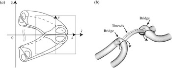
In the first phase, two vortices driven towards each other will deform to adopt an antiparallel configuration in the region near the reconnection position (Siggia Reference Siggia1985). In many reconnection problems, the vortices are initially placed so that they will interact in this antiparallel orientation, but in some cases, such as the problems of orthogonally offset vortices examined by Zabusky & Melander (Reference Zabusky and Melander1989) and Boratav, Pelz & Zabusky (Reference Boratav, Pelz and Zabusky1992), significant distortion of the vortices is required to attain the antiparallel configuration. Once in this antiparallel configuration, each vortex will induce a two-dimensional straining flow on the opposing vortex, and as a consequence the core of each vortex will become deformed and elongated. The curvature of the three-dimensional vortices along their axes serves both to drive the vortex cores into each other and to induce an additional background straining flow on the vortex pair, which causes each deformed core to develop a head–tail structure (Kida, Takaoka & Hussain Reference Kida, Takaoka and Hussain1991). As shown in figure 1(a), the ‘head’ is a region of increased thickness along the outside of the curved vortex core, and the inner part of the core stretches out to become the ‘tail’.

Figure 1.

(a) Deformation of vortex cores into a head–tail configuration (from Kida et al. Reference Kida, Takaoka and Hussain1991). (b) Simulation of the reconnection of a vortex pair performed using a triply periodic spectral method (from Marshall Reference Marshall2001), showing the direction of the induced velocity from cross-linked regions of the vortex cores and the vorticity threads left over from remnants of the core as the reconnected vortices move apart.

The second ‘bridging’ phase of vortex reconnection is dominated by the diffusive cross-cancellation of vorticity between the two antiparallel vortex cores. A simple model for this cross-cancellation process was proposed by Saffman (Reference Saffman1990), the predictions of which were compared to results of numerical simulations by Shelley et al. (Reference Shelley, Meiron and Orszag1993). As the opposite-sign vorticity cancels out due to diffusion between the two touching vortex cores, the vortex lines passing through the annihilated vorticity reconnect to those from the opposing vortex as a consequence of the requirement that the strength of a vortex tube remains uniform along the tube. These resulting bridges between the two vortex structures continue to grow stronger as more vorticity is diffusively annihilated within the vortex cores. However, since the vortex lines within these bridges are highly curved, their self-induced velocity increases as the bridges grow stronger, eventually causing them to propagate away from each other and discontinuing the vortex reconnection process before all vorticity within each vortex core has had a chance to diffusively interact with that in the opposing core.

The third phase of vortex reconnection deals with the remnants of vorticity, called threads, which are left behind as the bridges pull away from each other. As shown in figure 1(b), the threads have the form of a curved vortex pair, with a strength much less than that of the original vortex pair. The thread curvature is a result of both the self-induced velocity of the threads on each other and the velocity induced by the bridges. The thread curvature leads to a weak self-induced velocity that drives the threads towards each other, but this motion is also influenced by the straining flow induced by the bridges. The velocity induced by the bridges also causes strong stretching of the threads, which intensifies the vorticity within the thread cores. As a consequence of these various effects, the threads appear to remain in contact over a long time but the cross-diffusion between them is slow.

3. Numerical model

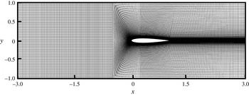
The Navier–Stokes equations were solved in primitive-variable form using a finite-volume method (Lai Reference Lai2000) and a block-structured mesh with hexahedral elements. The domain consisted of four implicitly coupled blocks and was designed to achieve high spatial resolution along the leading edge of the blade and along the blade boundary layer (figure 2). The simulation algorithm stores all dependent variables at the cell centres and calculates second-order-accurate approximations of the diffusive and convective fluxes on the cell boundaries. The momentum and continuity equations are coupled together using the PISO algorithm (Issa Reference Issa1985). To achieve additional numerical stability, the time derivative is weighted between a second-order derivative approximation and a first-order upwind with a 90:10 ratio.

Figure 2.

Cross-sectional view of the computational grid in the plane $z=0$ . The inlet and outlet planes are at $x=-3$ and $x=3$ , respectively, and the blade span length is equal to unity.

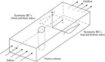
The computations were performed with a columnar vortex convected towards a fixed blade by a uniform upstream flow  $U$ . The Cartesian coordinate system used for these simulations was oriented such that the uniform flow was in the $x$ direction, the normal vector of the blade centre plane was in the $y$ direction and the blade span was in the $z$ direction (figure 3). Standard inflow and outflow boundary conditions were used for the boundary planes in the $x$ direction, and symmetry boundary conditions were used in the $y$ and $z$ directions. The blade was a NACA0012 airfoil with chord length $c$ and with leading edge lying on the line $x=0$ . The computational domain spanned the region $-3\leqslant x/c\leqslant 3$ , $-1\leqslant y/c\leqslant 1$ and $-1.25\leqslant z/c\leqslant 1.25$ , where the blade centre plane is given by the intersection of the blade with the $y=0$ plane. The initial velocity field was evaluated using a columnar Rankine vortex with uniform vorticity distribution, strength ${\it\Gamma}$ and core radius ${\it\sigma}_{0}/c=0.25$ , along with two similar vortices in neighbouring domains in the spanwise direction. The vortex axis was initialized on the central plane ( $z_{0}=0$ ) at a location $x_{0}/c=-1.1$ upstream of the blade leading edge, and the inlet plane was located upstream of the blade leading edge at $x_{\mathit{inlet}}/c=-3$ .

Figure 3.

Schematic diagram showing coordinate system and boundary conditions used for the numerical computations.

Several dimensionless parameters can be defined that govern orthogonal vortex–blade interactions. The vortex and blade Reynolds numbers are defined as $\mathit{Re}_{v}\equiv {\it\Gamma}/{\it\nu}$ and $\mathit{Re}_{B}\equiv Uc/{\it\nu}$ , where ${\it\nu}$ is the kinematic viscosity. The free-stream velocity $U$ can be used to define the impact parameter as $I\equiv 2{\rm\pi}{\it\sigma}_{0}U/{\it\Gamma}$ , which is the ratio of the relative vortex–blade velocity to the maximum swirl velocity within the vortex. 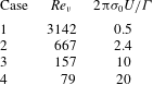The thickness parameter $T/{\it\sigma}_{0}$ , which is the ratio of the blade thickness $T$ to the vortex core radius  ${\it\sigma}_{0}$ , is important for determining the extent and type of vortex core deformation as the vortex approaches the blade. The ambient vortex axial flow was set to zero for all cases examined in the paper. The computations reported were selected to compare cases in the regime of high impact parameter and low thickness parameter. The values of these parameters for the cases considered in the paper are given in table 1. The thickness parameter is fixed at $T/{\it\sigma}_{0}=0.8$ and the blade Reynolds number is set at $\mathit{Re}_{B}=1000$ for all cases examined. The impact parameter varies from 0.5 to 20. In all instances, the impact parameter is sufficiently high that no separation of the boundary layer vorticity is observed prior to impact with the vortex. The vortex Reynolds number varies inversely with the impact parameter, ranging from 79 to 3142 for the different cases examined.

Table 1.

Values of the dimensionless parameters for the reported computations. The blade thickness parameter $T/{\it\sigma}_{0}=0.8$ and blade Reynolds number $\mathit{Re}_{B}=1000$ for all cases examined.

Typical values of blade and vortex Reynolds numbers in vortex cutting problems depend upon the application. Taking helicopter flow as an example system, for instance, the typical blade Reynolds number $\mathit{Re}_{B}$ is estimated by Leishman (Reference Leishman2006) as about $5\times 10^{6}$ for retreating blades and $2\times 10^{7}$ for advancing blades. The typical vortex strength is estimated by Leishman as being approximately equal to the bound vortex strength on the blade surface, which, for typical values of the blade solidity and thrust coefficient, gives helicopter vortex Reynolds numbers $\mathit{Re}_{v}$ of about 20 % of the blade Reynolds number. While these Reynolds-number values are much higher than those used in the current computations, it was shown by Liu & Marshall (Reference Liu and Marshall2004), and is also the case for vortex reconnection problems in general, that the value of the Reynolds number has only a minor influence on the vortex cutting flow results. For instance, Liu & Marshall (Reference Liu and Marshall2004) obtained computational results for blade lift coefficient during chopping of a vortex with axial flow which agree well with experimental values obtained at a Reynolds number three orders of magnitude higher than the computational value.

All length variables are non-dimensionalized using the blade chord $c$ , velocity variables are non-dimensionalized by the free-stream velocity $U$ , time is non-dimensionalized by the advective time $c/U$ , and vorticity is non-dimensionalized by the inverse time scale $U/c$ . Pressure and shear stress are non-dimensionalized by ${\it\rho}U^{2}$ , where ${\it\rho}$ is the fluid density. The blade surface vorticity flux, defined by

(3.1) $$\begin{eqnarray}\boldsymbol{q}=-{\it\nu}\frac{\partial {\bf\omega}}{\partial n},\end{eqnarray}$$

where $\boldsymbol{n}$ is the outward unit normal of the blade surface and ${\it\nu}$ is the kinematic viscosity, is non-dimensionalized by ${\it\nu}U/c^{2}$ .

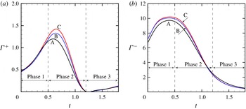
Grid independence was examined by repeating the calculation in case 2 for three different meshes, where the total number of grid points varied by a factor of 4.5 between the coarsest and finest meshes. The meshes are labelled as mesh A (865 536 grid points), mesh B (1900 701 grid points), and mesh C (3883 238 grid points). All computations in this comparison were performed with the same parameter values and with the same computational domain size. Grid independence was demonstrated by computing the positive and negative circulation measures, defined by

(3.2) $$\begin{eqnarray}\left.\begin{array}{@{}c@{}}\displaystyle {\it\Gamma}^{+}=\int _{L}{\it\omega}_{y}^{+}\,\text{d}x,\quad {\it\Gamma}^{-}=\int _{L}{\it\omega}_{y}^{-}\,\text{d}x,\\ \text{where}~{\it\omega}_{y}^{+}=\left\{\begin{array}{@{}ll@{}}{\it\omega}_{y}\quad & \text{if }{\it\omega}_{y}>0\\ 0\quad & \text{if }{\it\omega}_{y}\leqslant 0\end{array}\right.\quad \text{and}\quad {\it\omega}_{y}^{-}=\left\{\begin{array}{@{}ll@{}}0\quad & \text{if }{\it\omega}_{y}>0\\ -{\it\omega}_{y}\quad & \text{if }{\it\omega}_{y}\leqslant 0.\end{array}\right.\end{array}\right\}\end{eqnarray}$$

The line $L$ lies on the blade symmetry plane, extending over the interval $-1.3\leqslant x\leqslant 0$ upstream of the blade leading edge and passing through the ambient position of the vortex axis. The results are plotted as functions of time for each mesh type in figure 4. The peak negative circulation measure has about 4 % difference between meshes A and B, and less than 1 % difference between meshes B and C. The peak positive circulation measure has about 10 % difference between meshes A and B, and less than 5 % difference between meshes B and C. The negative values of ${\it\omega}_{y}$ lie within the vortex core, and the positive values of ${\it\omega}_{y}$ are induced within the thin blade boundary layer at the leading edge in response to the induced velocity by the vortex, which explains why the positive circulation measure is more sensitive to grid resolution than is the negative circulation measure. All subsequent computations in the paper were performed using the grid in mesh C. The three different phases of vortex cutting indicated in figure 4 are discussed in the next section.

Figure 4.

Positive and negative circulation measures, ${\it\Gamma}^{+}$ and ${\it\Gamma}^{-}$ , versus dimensionless time. The circulation was calculated along a line extending out from the blade front in the $x$ direction over the interval $-1.3\leqslant x\leqslant 0$ for three different meshes: mesh A, 865 536 grid points (black); mesh B, 1900 701 grid points (blue); and mesh C, 3883 238 grid points (red). The three phases of vortex reconnection are identified using dashed vertical lines.

The effect of domain size was also considered to ensure the accuracy of the numerical simulations. The most important parameter was found to be the distance between the initial position of the vortex core and the inlet plane. If this distance was set too small, the induced velocity from the vortex caused weak positive $y$ vorticity to be generated on the inlet plane, which propagates towards the blade behind the vortex. When this vorticity reaches the blade leading edge, it diffusively cancels with the uncut portion of the vortex core that was stretched around the blade leading edge. Several domains were examined, and the mesh in figure 2 was chosen in order to ensure that the strength of this inlet vorticity was small and that it did not reach the blade until very late in the computation. In addition, the effect of time step was considered and a dimensionless time step of 0.015 was chosen to ensure a Courant–Friedrichs–Lewy (CFL) number of less than unity.

4. Vortex cutting simulation results

The ambient vorticity within the vortex is in the negative $y$ direction. As the vortex approaches the blade, it induces a spanwise velocity that is associated with generation of vorticity in the positive $y$ direction along the blade leading edge. It is the diffusive cross-cancellation of the $y$ -oriented vorticity within the vortex with that in the boundary layer along the blade leading edge that controls the vortex cutting process, through which vortex lines within the vortex are cut and reconnect to vortex lines within the blade boundary layer.

4.1. Vorticity dynamics during vortex cutting

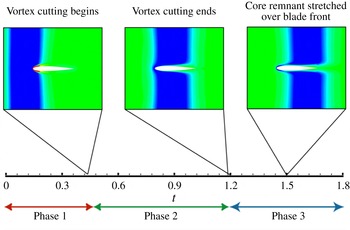
Throughout this section, detailed results are shown for case 2, and then comparisons of selected results for computations at other values of the impact parameter (listed in table 1) are given in § 4.2. A timeline of the basic vortex cutting process is given in figure 5, in which contour plots of ${\it\omega}_{y}$ are shown in the $x{-}y$ plane for three times to illustrate the position of the vortex core relative to the blade during different phases of the vortex cutting process. Both figure 5 and the positive and negative circulation plots in figure 4 indicate three phases of vortex cutting, which correspond to the three phases of vortex reconnection discussed by Melander & Hussain (Reference Melander and Hussain1989).

Figure 5.

Timeline of the vortex cutting process, showing the three phases of vortex reconnection.

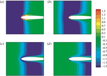
A close-up plot is given in figure 6, showing the ${\it\omega}_{y}$ values within a region near the blade leading edge, where regions with high negative values of ${\it\omega}_{y}$ are shown in blue and regions with high positive values of ${\it\omega}_{y}$ are shown in red. In the first phase of vortex cutting, the vortex interacts with the inviscid flow induced by the blade, and the front part of the vortex deforms slightly, bending around the blade. Also during this phase, the vortex induces formation of a region of positive ${\it\omega}_{y}$ within the blade leading-edge boundary layer. Phase 2 begins when the vortex impacts with the blade boundary layer, so that the regions with positive and negative values of ${\it\omega}_{y}$ , within the blade boundary layer and the vortex core, respectively, interact by diffusion and partially annihilate each other. This viscous cross-diffusion leads to a rapid decrease in both the negative and positive circulation measures, as shown in figure 4 during the phase 2 time interval, and causes the vortex lines in the vortex core to break and reconnect to those in the blade boundary layer. Phase 3 occurs for times greater than about $t=1.2$ , for which the value of ${\it\omega}_{y}$ within the blade boundary layer changes from positive to negative. As demonstrated by Liu & Marshall (Reference Liu and Marshall2004), this change in sign is associated with the fact that, as the blade leading edge passes through the core, the induced spanwise velocity along the leading edge changes direction. 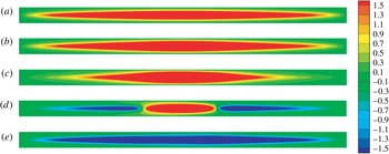After the change in sign of ${\it\omega}_{y}$ within the blade boundary layer occurs, the $y$ component of vorticity within the core is of the same sign as that within the blade boundary layer and diffusive annihilation can no longer occur. A series of plots showing how the value of ${\it\omega}_{y}$ along the blade leading edge changes sign is given in figure 7, for a similar time frame as in figure 6 but viewed looking along the $x$ direction, directly towards the blade front region. From this figure, we see that the change in sign of ${\it\omega}_{y}$ first occurs at the ends of the blade span and then moves towards the blade centre as time progresses.

Figure 6.

Contour plots from case 2 showing a close-up of ${\it\omega}_{y}$ near the blade from a slice along the blade centre span in the $x{-}y$ plane for (a) $t=0.75$ , (b) 1.05, (c) 1.35 and (d) 1.65.

Figure 7.

Contour plots from case 2 of ${\it\omega}_{y}$ on the front of the blade for (a) $t=0.15$ , (b) 0.45, (c) 0.75, (d) 1.05 and (e) 1.35.

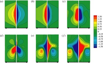
The $x$ component of vorticity also undergoes a sign change as the vortex core passes over the leading edge of the blade. Initially, the induced spanwise velocity from the vortex causes a region of positive ${\it\omega}_{x}$ to form on the blade top and a region of negative ${\it\omega}_{x}$ on the blade bottom. As the vortex passes over a given point on the blade surface, the induced spanwise velocity at that point changes direction, resulting in a change in the sign of ${\it\omega}_{x}$ . Plots illustrating this effect using a time series of contours of ${\it\omega}_{x}$ are shown on the cross-sectional plane $z=0$ (figure 8) and on projections of the blade top and bottom surfaces looking along the $y$ axis (figure 9). The change in sign of ${\it\omega}_{x}$ closely follows the path of the vortex core.

Figure 8.

Contour plots from case 2 of ${\it\omega}_{x}$ from a slice along the blade centre span in the $x{-}y$ plane for (a) $t=0.75$ , (b) 1.05, (c) 1.35 and (d) 1.65.

Figure 9.

Contour plots from case 2 of ${\it\omega}_{x}$ on the blade top (left) and bottom (right) at (a)  $t=0.15$ , (b) 0.45, (c) 0.75, (d) 1.05, (e) 1.35 and (f) 1.65.

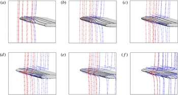
The essence of vortex reconnection involves cutting of vortex lines originating from one vorticity region and reconnection to vortex lines originating from another vorticity region via diffusion-regulated annihilation of vorticity between the two regions. This vortex line reconnection process for the vortex cutting problem is illustrated in figure 10 for a time series as the blade penetrates into the vortex core. In order to illustrate the vortex reconnection process, we colour the vortex lines red to indicate vortex lines that originate within the vortex and remain within the vortex, black to indicate vortex lines that originate within the blade boundary layer and remain within the boundary layer, and blue to indicate vortex lines that originate within the vortex and cross over to join those within the blade boundary layer (or vice versa). Near the beginning of this sequence, the sign of ${\it\omega}_{y}$ is positive at the blade leading edge, and vorticity annihilation between the boundary layer and the vortex allows the vortex lines within the core to cut and reconnect to those within the boundary layer, increasing the number of blue lines. As the vortex core centre passes the position of the blade leading edge, the value of ${\it\omega}_{y}$ at the leading edge changes sign. Vortex lines from the vortex (in red) now begin to deform and to stretch in the spanwise direction instead of being cut. The pattern change of the black vortex lines illustrates how the vorticity orientation in the boundary layer along the front section of the blade changes as the vortex core passes over the blade leading edge.

Figure 10.

Oblique view of the vortex cutting process. Vortex lines originating in the vortex core can either remain within the vortex core (red) or be cut and reconnect to vortex lines in the boundary layer (blue). Similarly, vortex lines originating within the blade boundary layer can either stay in the boundary layer (black) or join to those originating within the core (blue). Images are shown at times (a) $t=0.75$ , (b) 0.90, (c) 1.05, (d) 1.20, (e) 1.35 and (f) 1.50. The (uncut) red vortex lines near the blade leading edge become deflected in the spanwise direction as they near the blade.

Figure 11.

Pressure contours in the $x{-}y$ plane passing through the centre span of the blade for (a) $t=0.3$ , (b) 0.6, (c) 0.9 and (d) 1.2. The outlines of the vortex are shown by plotting vortex lines on the two sides of the vortex.

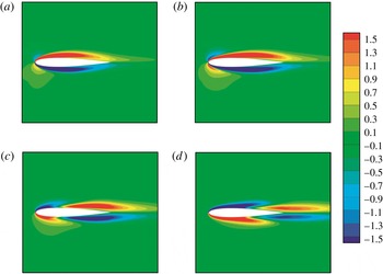
The pressure change along the vortex core caused by the presence of the blade is another important aspect of the vortex cutting process. For reconnection of two antiparallel vortex tubes, Saffman (Reference Saffman1990) proposed that the localized increase in vortex core pressure creates a positive feedback loop to drive the vortex reconnection process. We examined how the pressure in the vortex core changed for vortex cutting in order to understand if pressure plays a similar role in the vortex cutting problem. Figure 11 illustrates the pressure in the vortex core for a contour plot in the $z=0$ plane, passing through the centre span of the blade. Initially there is a large region of low pressure in the vortex core as well as on the top and bottom surfaces of the blade and a region of high pressure around the blade leading edge. As the vortex moves closer to the blade, the pressure in the vortex core increases close to the impingement region and a pressure gradient forms. This phenomenon is similar to the one Saffman (Reference Saffman1990) described, but it occurs for a different reason. In the case of vortex cutting by a blade, the impingement of the vortex upon the ambient high pressure near the blade leading edge no doubt plays a significant role in driving the localized pressure gradient along the vortex core, and any role that core deformation might play in this process is obscured. As the vortex passes over the blade, the low-pressure region in the vortex core connects with the low-pressure regions on the top and bottom surfaces of the blade, as shown in figure 11(c,d).

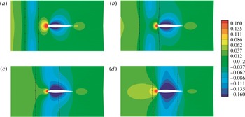
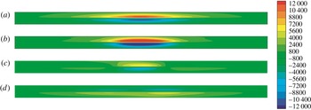
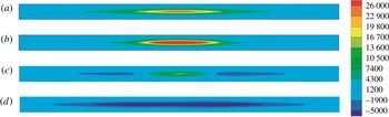
The key difference between vortex cutting by a blade and more traditional vortex reconnection is the fact that vorticity is generated on the blade surface, which lies within the region dominated by vorticity diffusive interaction. The $x$ and $y$ components of the surface vortex flux, $q_{x}$ and $q_{y}$ , are shown within a projection of the front region of the blade (looking along the $x$ axis) in figures 12 and 13. The vorticity flux contour plots exhibit a change in sign around $t=1.05$ , which corresponds with the change in sign of ${\it\omega}_{x}$ and ${\it\omega}_{y}$ during vortex passage previously discussed in this section. The contour plots show that the vorticity flux is primarily generated within the leading-edge region of the blade, and not on the blade top and bottom surfaces away from the leading edge. This region is exactly where the breaking and rejoining of vortex lines occur, and further demonstrates the importance of considering the role of surface vorticity flux in a blade–vortex cutting problem.

Figure 12.

Contour plots of the $x$ component of the vorticity flux, $q_{x}$ , on the blade leading edge, at times (a) $t=0.45$ , (b) 0.75, (c) 1.05 and (d) 1.35.

Figure 13.

Contour plots of the $y$ component of the vorticity flux, $q_{y}$ , on the blade leading edge, at times (a) $t=0.45$ , (b) 0.75, (c) 1.05 and (d) 1.35.

4.2. Effect of impact parameter

Plots of the time variation of the maximum and minimum values of vorticity and surface vorticity flux are shown for all four cases examined in figures 14 and 15 in order to better understand the effect of impact parameter on the temporal changes in these quantities throughout the vortex cutting process and the manner in which the vortex cutting process changes with respect to the impact parameter. In interpreting these plots, it is helpful to keep in mind the time intervals for major transitions in the cutting process, namely, the onset of penetration of the blade leading edge into the vortex core ( $t\cong 0.45$ ), the passage of the blade leading edge out of the opposite side of the vortex position ( $t\cong 1.2$ ) and stretching of vortex remnants over the blade leading edge ( $t>1.2$ ). These three time intervals correspond approximately to the three phases of traditional vortex tube reconnection as described in § 2.

Figure 14.

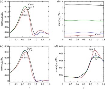
Time variation plots of (a) maximum ${\it\omega}_{x}$ , (b) maximum ${\it\omega}_{z}$ , (c) maximum ${\it\omega}_{y}$ and (d) minimum ${\it\omega}_{y}$ , normalized with respect to the vortex Reynolds number, $\mathit{Re}_{v}={\it\Gamma}/{\it\nu}$ . Results are shown for cases 1 (red), 2 (blue), 3 (green) and 4 (black).

Figure 15.

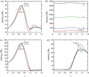
Time variation plots of the maximum values of the surface vorticity flux components (a) $q_{x}$ , (b) $q_{z}$ and (c) $q_{y}$ , and minimum values of (d) $q_{y}$ , normalized with respect to the vortex Reynolds number. Results are shown for cases 1 (red), 2 (blue), 3 (green) and 4 (black).

Figure 14 shows the time variation of the maximum values of ${\it\omega}_{x}$ and ${\it\omega}_{z}$ , normalized with respect to the vortex Reynolds number, $\mathit{Re}_{v}$ . The minimum values of these vorticity components follow nearly identical profiles as the maximum values owing to the symmetry on the top and bottom surfaces of the blade, and so are not plotted. The different cases considered differ from each other by the value of the vortex strength, leading to different values of the vortex Reynolds number and vortex–blade impact parameter. However, the plots of maximum and minimum normalized ${\it\omega}_{x}$ values for these different cases appear to nearly collapse onto a single curve, although with a slight deviation for case 1. The plot in figure 14(a) exhibits an increase in ${\it\omega}_{x}$ with time until around $t=0.75$ , which corresponds to the time at which the vortex core axis passes over the blade leading edge. Following this time, the value of ${\it\omega}_{x}$ gradually decreases until it approaches its initial value as the vortex moves past the tail end of the blade. The maximum value of ${\it\omega}_{x}$ occurs in the centre of the blade, slightly above the blade centre plane but within the blade boundary layer. From figure 14(a), we conclude that the maximum value of ${\it\omega}_{x}$ is dominated by the initial cutting of the vortex, and that this value increases approximately linearly with the vortex strength.

The maximum value of ${\it\omega}_{z}/\mathit{Re}_{v}$ , shown in figure 14(b), clearly does not collapse onto a single curve for the different cases examined. The results for the different cases appear to be qualitatively similar, but the maximum value of ${\it\omega}_{z}/\mathit{Re}_{v}$ increases (decreases) as the vortex Reynolds number increases (decreases). The maximum in ${\it\omega}_{z}$ also occurs at a somewhat later time than does the maximum in ${\it\omega}_{x}$ , although it seems to occur at the same time for all of the cases examined. In contrast to the maximum of ${\it\omega}_{x}$ , the maximum value of ${\it\omega}_{z}$ occurs to the left of the centre of the blade span and slightly below the blade centre plane. This shift is probably due to the induced velocity of the vortex creating a slightly higher free-stream velocity on the left side of the blade and slightly lower velocity on the right side, looking downwind towards the blade leading edge.

The maximum and minimum values of ${\it\omega}_{y}$ , normalized by the vortex Reynolds number, are plotted in figure 14(c,d) for the four cases listed in table 1, each with a different value of the impact parameter. We again see that the curves nearly coincide for the different cases examined, with the exception of a slight deviation for case 1. This data collapse indicates that the value of ${\it\omega}_{y}$ varies approximately linearly with vortex strength. The maximum positive value of ${\it\omega}_{y}$ (which occurs within the boundary layer at the blade leading edge) initially increases as the blade penetrates into the vortex core until a time of about $t=0.75$ , and after which it decreases to a value of nearly zero as the vortex core passes over the leading edge of the blade and the positive vorticity on the blade front induced by the vortex changes sign. The maximum negative value of ${\it\omega}_{y}$ , which initially occurs within the vortex core, exhibits a gradual decay with time during the initial part of the computation, which is due to viscous diffusion of the vortex core. The maximum negative value of ${\it\omega}_{y}$ is not significantly effected by the vortex cutting process until the vortex core moves past the blade leading edge and the value of ${\it\omega}_{y}$ within the blade boundary layer changes from a positive to a negative sign. From this time until the end of the computation, the point of maximum negative value of ${\it\omega}_{y}$ is located at the blade leading edge. The maximum negative value of ${\it\omega}_{y}$ gradually increases from the time ( $t=0.75$ ) of change in sign of ${\it\omega}_{y}$ within the blade boundary layer to a time at which the blade leading edge has entirely penetrated through the vortex core (about $t=1.5$ ), after which the maximum negative value of ${\it\omega}_{y}$ remains approximately constant for the remainder of the computation. Both the generation of negative ${\it\omega}_{y}$ due to induced spanwise velocity from the vortex and the increase in vorticity due to stretching of the remaining portions of the vortex wrapped about the blade leading edge contribute to producing the maximum negative ${\it\omega}_{y}$ value. The fact that the peak value of the maximum negative value of ${\it\omega}_{y}$ occurs quite late, when the vortex core is well past the centre of the blade, suggests the presence of significant uncut vorticity remnants from the impinging vortex. These uncut vorticity remnants wrap around the blade surface in the form of a thin vortex sheet, for which the value of the negative-vorticity component ${\it\omega}_{y}$ continuously intensifies by stretching about the blade leading edge, while at the same time it is regulated by viscous diffusion, eventually approaching a constant value in a manner analogous to the classical Burgers vortex (Burgers Reference Burgers1948).

The time variation in the positive and negative components of the surface vorticity flux is shown in figure 15. The $x$ and $z$ vorticity fluxes, $q_{x}$ and $q_{z}$ , exhibit a functional form very similar to the corresponding maximum values of the vorticity components ${\it\omega}_{x}$ and ${\it\omega}_{z}$ . As was the case for the vorticity, the maximum positive and negative values of the vorticity flux in these directions follow the same curve, and the maximum values of $q_{x}$ for the different cases examined collapse nearly onto a single curve, while those for $q_{z}$ do not. We again see an initial increase in the positive-vorticity flux component $q_{y}$ , which then drops off to zero as the cutting process stops, and a late increase in the negative component of vorticity flux as negative $y$ vorticity is generated on the blade leading edge.

5. Model for vortex sheet in a straining flow near a surface

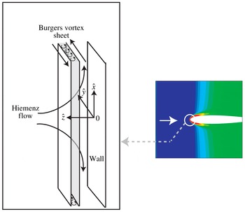
A key component of the vortex cutting process involves diffusive vorticity annihilation between the incident vortex and vorticity generated on the blade boundary layer. The incident vorticity initially has the form of a tube, but, as it wraps about the blade leading edge, it deforms into more of a sheet-like structure (Marshall & Grant Reference Marshall and Grant1996). Finally, the stretching of the impinging vortex imposed by the ambient flow about the blade leading edge plays a critical role in determining the vorticity evolution within the cutting region. In this section we describe a new exact Navier–Stokes solution that contains these three elements – antiparallel vorticity diffusive annihilation, vorticity generation on a surface, and vortex stretching. While the model to be presented incorporates these three key elements, to make the problem analytically tractable, we must dramatically modify certain other elements of the vortex cutting problem. In particular, the model does not deal with vorticity bending around the highly curved blade leading edge, but instead considers vorticity above a flat surface that is stretched by an imposed viscous straining flow (Hiemenz Reference Hiemenz1911), as indicated in the schematic diagram in figure 16. Secondly, the vortex sheet is assumed to be infinitely wide, whereas the incident vortex in the vortex cutting problem has a finite width. Were it not for the presence of the solid surface, this stretched vortex sheet would be identical to a Burgers sheet, where the vorticity within the sheet is oriented along the direction of the straining flow (Burgers Reference Burgers1948; Gibbon, Fokas & Doering Reference Gibbon, Fokas and Doering1999). Because of these various simplifications incorporated into the model, we do not expect the model solutions to provide an accurate quantitative approximation of the vorticity field in the problem of vortex cutting by a blade. Nevertheless, the model contains many of the key ingredients of the vortex cutting problem and it may be helpful in suggesting physically motivated scaling for the vortex cutting problem. As an exact Navier–Stokes solution, the model is also of interest in its own right.

Figure 16.

(a) Schematic diagram of the model flow field, consisting of a Burgers vortex sheet (shaded) immersed in a Hiemenz straining flow. (b) Illustration of vertical vorticity contours during vortex–blade interaction, showing the relationship between the model flow and vorticity dynamics occurring at the blade leading edge during the vortex cutting process.

The model deals with a combination of a Hiemenz straining flow and a vortex sheet over a flat surface. The model problem is solved using the Cartesian coordinate system ( $\hat{x},{\hat{y}},\hat{z}$ ) shown in figure 16, in which $\hat{z}$ points in the upstream direction, $\hat{x}$ is oriented in the direction of the Heimenz straining flow close to the wall, and ${\hat{y}}$ is in the direction of the flow induced by the vortex sheet. Figure 16 illustrates the fact that this model is intended to be representative not of the entire vortex–blade interaction problem, but only of the flow very close to the point of vortex impingement on the blade leading edge. The velocity and pressure fields are assumed to satisfy

(5.1a,b ) $$\begin{eqnarray}\boldsymbol{u}=\hat{u} (\hat{x},\hat{z})\boldsymbol{e}_{\hat{x}}+\hat{v}(\hat{z},t)\boldsymbol{e}_{{\hat{y}}}+{\hat{w}}(\hat{z})\boldsymbol{e}_{\hat{z}},\quad p=p_{1}(\hat{x})+p_{2}(\hat{z}).\end{eqnarray}$$

Under these conditions, the continuity and Navier–Stokes equations reduce to

(5.2a ) $$\begin{eqnarray}\displaystyle & \displaystyle \frac{\partial \hat{u} }{\partial \hat{x}}+\frac{\partial {\hat{w}}}{\partial \hat{z}}=0, & \displaystyle\end{eqnarray}$$

(5.2b ) $$\begin{eqnarray}\displaystyle & \displaystyle \hat{u} \frac{\partial \hat{u} }{\partial \hat{x}}+{\hat{w}}\frac{\partial \hat{u} }{\partial \hat{z}}=-\frac{1}{{\it\rho}}\frac{\partial p_{1}}{\partial \hat{x}}+{\it\nu}\left(\frac{\partial ^{2}\hat{u} }{\partial \hat{x}^{2}}+\frac{\partial ^{2}\hat{u} }{\partial \hat{z}^{2}}\right), & \displaystyle\end{eqnarray}$$

(5.2c ) $$\begin{eqnarray}\displaystyle & \displaystyle \frac{\partial \hat{v}}{\partial t}+{\hat{w}}\frac{\partial \hat{v}}{\partial \hat{z}}={\it\nu}\frac{\partial ^{2}\hat{v}}{\partial \hat{z}^{2}}, & \displaystyle\end{eqnarray}$$

(5.2d ) $$\begin{eqnarray}\displaystyle & \displaystyle {\hat{w}}\frac{\partial {\hat{w}}}{\partial \hat{z}}=-\frac{1}{{\it\rho}}\frac{\partial p_{2}}{\partial \hat{z}}+{\it\nu}\,\,\frac{\partial ^{2}{\hat{w}}}{\partial \hat{z}^{2}}. & \displaystyle\end{eqnarray}$$

We denote the straining rate of the external Hiemenz flow by $s$ , the strength of the Burgers vortex sheet by ${\it\gamma}$ , a scaled height variable by ${\it\eta}=\hat{z}\sqrt{s/{\it\nu}}$ , and a scaled time by ${\it\tau}=st$ . The velocity components can be written as

(5.3a−c ) $$\begin{eqnarray}\hat{u} =s\hat{x}F^{\prime }({\it\eta}),\quad \hat{v}={\it\gamma}G({\it\eta},{\it\tau}),\quad {\hat{w}}=-F({\it\eta})\sqrt{s{\it\nu}}.\end{eqnarray}$$

These expressions for velocity satisfy the continuity equation (5.2a ) identically, and the momentum equations (5.2b ) and (5.2d ) reduce to an ordinary differential equation for $F({\it\eta})$ as

(5.4) $$\begin{eqnarray}F^{\prime \prime \prime }+FF^{\prime \prime }-(F^{\prime })^{2}+1=0,\end{eqnarray}$$

subject to the boundary conditions $F(0)=F^{\prime }(0)=0$ and $F^{\prime }(\infty )=1$ . Substituting (5.3a−c ) into (5.2c ) yields a partial differential equation for $G({\it\eta},{\it\tau})$ as

(5.5) $$\begin{eqnarray}\frac{\partial G}{\partial {\it\tau}}-F({\it\eta})\frac{\partial G}{\partial {\it\eta}}=\frac{\partial ^{2}G}{\partial {\it\eta}^{2}}.\end{eqnarray}$$

Equation (5.5) is subject to the boundary conditions

(5.6a,b ) $$\begin{eqnarray}G(0,{\it\tau})=0,\quad G(\infty ,{\it\tau})={\it\alpha},\end{eqnarray}$$

where ${\it\alpha}$ is a prescribed parameter representing the ratio of the velocity far away from the plate to the vortex sheet strength.

Equation (5.4) is equivalent to the classic Hiemenz problem, which was solved using a fourth-order Runge–Kutta method, yielding $F^{\prime \prime }(0)=1.23259$ . Equation (5.5) was solved using the Crank–Nicolson method with ${\rm\Delta}{\it\eta}=0.005$ and ${\rm\Delta}{\it\tau}=0.001$ . The primary dimensionless parameter is the ratio ${\it\alpha}$ of velocity $\hat{v}_{\infty }$ in the ${\hat{y}}$ direction far away from the surface to the initial vortex sheet strength ${\it\gamma}$ . Other parameters include the initial position ${\it\eta}_{0}$ of the vortex sheet and the initial thickness ${\it\Delta}$ of the Stokes first problem boundary layer on the wall. A simple example calculation is considered using this model for the problem of a vortex sheet being driven into a flat wall by a Hiemenz straining flow. The initial condition for this example problem has the form of an equilibrium Burgers vortex sheet centred at ${\it\eta}_{0}$ and a Stokes first problem boundary layer with dimensionless thickness ${\it\Delta}$ , given by

(5.7) $$\begin{eqnarray}G({\it\eta},0)=G_{0}({\it\eta})=(1+{\it\alpha})\,\text{erf}({\it\eta}/2{\it\Delta})-{\textstyle \frac{1}{2}}-{\textstyle \frac{1}{2}}\,\text{erf}[({\it\eta}-{\it\eta}_{0})/\sqrt{2}],\end{eqnarray}$$

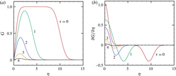
where erf( $\cdot$ ) is the error function. For this example problem, we chose ${\it\eta}_{0}=10$ and ${\it\Delta}=1$ . Results for this flow are shown in figure 17 for the dimensionless velocity $G=\hat{v}/{\it\gamma}$ and dimensionless vorticity ${\it\zeta}\equiv \partial G/\partial {\it\eta}$ as functions of dimensionless time ${\it\tau}$ . Based on the coordinate system shown in figure 16, the velocity is in the ${\hat{y}}$ direction and the vorticity is in the $\hat{x}$ direction. Dimensionless circulation measures ${\it\Gamma}^{+}$ and ${\it\Gamma}^{-}$ are defined by

(5.8) $$\begin{eqnarray}\left.\begin{array}{@{}c@{}}\displaystyle {\it\Gamma}^{+}=\int _{L}{\it\zeta}^{+}\,\text{d}{\it\eta},\quad {\it\Gamma}^{-}=\int _{L}{\it\zeta}^{-}\,\text{d}{\it\eta},\\ \displaystyle \text{where}~{\it\zeta}^{+}=\left\{\begin{array}{@{}ll@{}}{\it\zeta}\quad & \text{if }{\it\zeta}>0\\ 0\quad & \text{if }{\it\zeta}\leqslant 0\end{array}\right.\quad \text{and}\quad {\it\zeta}^{-}=\left\{\begin{array}{@{}ll@{}}0\quad & \text{if }{\it\zeta}>0\\ -{\it\zeta}\quad & \text{if }{\it\zeta}\leqslant 0,\end{array}\right.\end{array}\right\}\end{eqnarray}$$

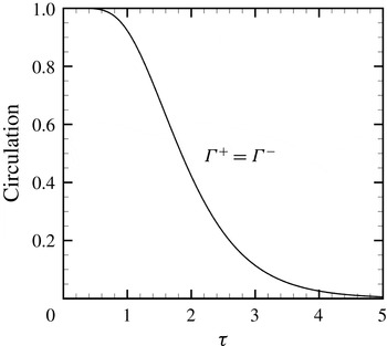
and $L$ denotes the range ( $0,{\it\eta}_{\mathit{max}}$ ) of ${\it\eta}$ . Plots of time variation of ${\it\Gamma}^{+}$ and ${\it\Gamma}^{-}$ , given for the example problem in figure 18, provide a quantitative measure of the extent of vorticity diffusion-driven annihilation occurring between the incident vortex sheet and the boundary layer vorticity.

Figure 17.

Variation of (a) the dimensionless velocity $G$ and (b) the dimensionless vorticity $\partial G/\partial {\it\eta}$ as functions of ${\it\eta}$ for a case with ${\it\alpha}=0$ . Plots are shown for ${\it\tau}=0$ (red), 1 (green), 2 (blue), 3 (orange), and 4 (black).

Figure 18.

Time variation of dimensionless circulation measures, ${\it\Gamma}^{+}$ and ${\it\Gamma}^{-}$ , as functions of ${\it\tau}$ for the example problem shown in figure 17. For the case with ${\it\alpha}=0$ , ${\it\Gamma}^{+}={\it\Gamma}^{-}$ .

Figure 19.

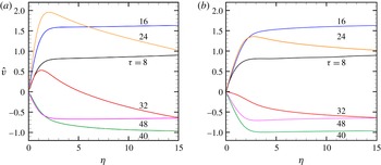
Comparison of profiles of dimensionless velocity $\hat{v}$ as a function of ${\it\eta}$ at ${\it\tau}=8$ (black), 16 (blue), 24 (orange), 32 (red), 40 (green) and 48 (purple). Plots are shown for (a) the vortex cutting simulation described in § 4 and (b) the simple model described in § 5.

In the numerical simulation of vortex cutting by a blade discussed in § 4, the assumption that the ambient flow past the blade has the form of a plane straining flow would only be relevant in a region close to the blade leading edge. While we do not expect this simple model to provide an accurate quantitative description of the full numerical simulation, it is nevertheless of interest to compare the model results with those of the full numerical simulation within this near-blade region. In comparing these results, we note the relationships $(\hat{x},{\hat{y}},\hat{z})=(y,-z,-x)$ and $(\hat{u} ,\hat{v},{\hat{w}})=(v,-w,-u)$ between coordinate and velocity components in the model problem and the numerical simulation. The value of the spanwise velocity component $w$ was extracted from the numerical simulations along a line corresponding to the $x$ axis from $x=0$ to $x=-15\sqrt{s/{\it\nu}}$ , corresponding to the interval $0\leqslant {\it\eta}\leqslant 15$ . The straining rate $s$ was obtained by extracting the velocity component $v$ in the $y$ direction along this same line and fitting a tangent line near ${\it\eta}=0$ , which for case 2 yields $s=26.7$ . The negative spanwise velocity ( $-w$ ) extracted along this line is comparable to the velocity component $\hat{v}$ in the simple theoretical model, and it is plotted as a function of ${\it\eta}$ in figure 19(a) for different values of the scaled time variable ${\it\tau}=st$ . Comparison results for the theoretical model in figure 19(b) were obtained using the same initial velocity profile as shown in figure 19(a) for the vortex cutting simulation, and by varying the boundary condition ${\it\alpha}$ in (5.6a,b ) as a function of time in accordance with the values of $\hat{v}$ at the position ${\it\eta}=15$ along the extraction line obtained from the vortex cutting simulation. The model calculation was initialized at ${\it\tau}=8$ in order to give the vortex time to approach the blade surface. The results from the model calculations are plotted in figure 19(b) for the velocity profile. The two sets of results do not exactly match up, but they have sufficiently good qualitative similarities to suggest that the temporal and spatial scaling suggested by the model are valid also with more general vortex cutting problems. To quantify the vorticity annihilation in the vortex cutting simulations and the simple model, we plot in figure 20 the time variation of the positive and negative circulation measures, ${\it\Gamma}^{+}$ and ${\it\Gamma}^{-}$ , which are computed in this case using integration over the interval $0\leqslant {\it\eta}\leqslant 15$ , corresponding to the interval $-0.09\leqslant x\leqslant 0$ in the numerical simulations of vortex cutting by a blade. We observe higher peaks of both the positive and negative circulation for the vortex cutting simulations compared to the simple model, which is probably an effect of the strong curvature of the vortex around the blade leading edge in the vortex cutting simulations. The qualitative features of the two plots, including the vorticity variation on the time scale ${\it\tau}$ and the manner in which the stretched vorticity within the flow interacts with and is annihilated by vorticity generated at the surface, appear to be similar between the model and the full simulations.

Figure 20.

Time variation of the dimensionless circulation measures, ${\it\Gamma}^{+}$ and ${\it\Gamma}^{-}$ , as functions of ${\it\tau}$ for the vortex cutting problem shown in figure 19. Plots are shown for (a) the vortex cutting simulation described in § 4 and (b) the simple model described in § 5.