





1 Introduction
Cellular automata (CAs) are a class of discrete dynamical systems consisting of an infinite line (or, more generally, a multidimensional grid) of ‘cells’, each of which holds one of finitely many states. Each cell evolves by an identical rule, and its next state is determined by the current state of itself and some finite set of neighbouring cells. The 256 elementary cellular automata (ECAs) [Reference Wolfram11] are those with only two states and neighbourhood
${N = \{-1,0,1\}}$
 , meaning that each cell can communicate only with its nearest neighbours. They are arguably the simplest CAs that exhibit complex dynamics.
We focus on the dynamics of elementary CA number 18. It has been studied as a model of mutually annihilating particles with random movement as early as 1983 [Reference Grassberger3] and by several authors since [Reference Jen5, Reference Kůrka6]. Grassberger [Reference Grassberger3] and Lind [Reference Lind8] conjectured that if the CA is initialized from a uniformly random configuration, then the density of particles almost surely decreases to zero with the same speed as mutually annihilating independent random walks. Progress towards the conjecture has been slow. Kůrka claimed in [Reference Kůrka6] that the density indeed approaches zero, but we show that the presented proof is faulty (see the discussion after Proposition 4.5).
The long-term fate of a dynamical system can be studied via its limit set, or eventual image. The limit set of a CA often contains transient phenomena, so several variants have been proposed to better capture the intuitive notion of ‘what typically happens after a long time’. These include the
$\mu $
 -limit set [Reference Kůrka and Maass7] and the generic limit set, introduced by Milnor in [Reference Milnor9] and studied first in the context of CAs in [Reference Djenaoui and Guillon2]. As our main results, we characterize the words with at most two particles that occur in the generic limit set of rule 18 and show that the three limit sets are all distinct. We also show that determining the generic limit set of rule 18 is a viable strategy towards (partially) resolving the conjecture of Grassberger and Lind.
2 Definitions
Let A be a finite alphabet. The set of finite words over A is denoted by
$A^*$
 and concatenation of words
$v, w \in A^*$
 is denoted by either
$v w$
 or
$v \cdot w$
 . This notation is extended to infinite words: if
$v \in A^*$
 and
$x \in A^{\mathbb {N}}$
 is a right-infinite word, then
$v x \in A^{\mathbb {N}}$
 ; if
$y \in A^{-\mathbb {N}}$
 is a left-infinite word, then
$y v \in A^{-\mathbb {N}}$
 ; and
$y x \in A^{\mathbb {Z}}$
 is a bi-infinite word. The full shift is the set
$A^{\mathbb {Z}}$
 of all bi-infinite sequences over A, equipped with the prodiscrete topology, which is generated by the cylinder sets
$[w]_i = \{x \in A^{\mathbb {Z}} \mid x_{[i, i+|w|-1]} = w\}$
 for
$w \in A^*$
 and
$i \in \mathbb {Z}$
 . The shift map
$\sigma : A^{\mathbb {Z}} \to A^{\mathbb {Z}}$
 is defined by
$\sigma (x)_i = x_{i+1}$
 . A subshift is a topologically closed set
$X \subseteq A^{\mathbb {Z}}$
 that is shift-invariant:
$\sigma (X) = X$
 . A word
$w \in A^*$
 occurs in X if
$X \cap [w]_0 \neq \emptyset $
 . The language of X is the set of words occurring in it; a subshift is defined by its language.
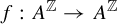
A CA is a continuous function
$f : A^{\mathbb {Z}} \to A^{\mathbb {Z}}$
 that commutes with the shift:
${f \circ \sigma = \sigma \circ f}$
 . By the Curtis–Hedlund–Lyndon theorem [Reference Hedlund4], every CA has a finite radius
$r \geq 0$
 and a local rule
$F : A^{2r+1} \to A$
 such that
$f(x)_i = F(\sigma ^i(x)|_{[-r,r]})$
 for all
$x \in A^{\mathbb {Z}}$
 and
$i \in \mathbb {Z}$
 . Once r is fixed, we can apply the CA to words
$w \in A^n$
 as well as configurations:
$f(w) = F(w_{[0,2r]} w_{[1,2r+1]} \cdots w_{[n-2r-1,n-1]})$
 . Note that each application of f shortens the word by
$2r$
 symbols.
The ECAs, defined in [Reference Wolfram11], are those with alphabet
$A = \{0,1\}$
 and radius
$1$
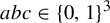
 . They are numbered from 0 to 255: the local rule F of ECA n maps
$a b c \in \{0,1\}^3$
 to bit number
$4a + 2b + c$
 in the binary representation of n (extended to three digits by prepending zeros if necessary).
A topological dynamical system is a pair
$(X, T)$
 , where X is a compact metric space and
$T : X \to X$
 is a continuous function. CAs are examples of such systems.
A Borel probability measure on a topological space X is a function
$\mu : \mathcal {B}(X) \to [0,1]$
 , where
$\mathcal {B}(X)$
 is the class of Borel subsets of X, satisfying
$\mu (X) = 1$
 ,
$\mu (\emptyset ) = 0$
 and
$\mu (\bigcup _{n \in \mathbb {N}} X_n) = \sum _{n \in \mathbb {N}} \mu (X_n)$
 whenever the sets
$X_n$
 are pairwise disjoint. The set of Borel probability measures of X is denoted
$\mathcal {M}(X)$
 . The support of
$\mu \in \mathcal {M}(X)$
 is the smallest closed subset
 with measure
$1$
 . If
$(X,T)$
 is a dynamical system, the dynamics T can be extended to a function
$T : \mathcal {M}(X) \to \mathcal {M}(X)$
 by
$(T \mu )(K) = \mu (T^{-1}(K))$
 . We denote by
$\mathcal {M}_T(X)$
 the subset of measures that are T-invariant, meaning
$T \mu = \mu $
 . A measure
$\mu \in \mathcal {M}_T(X)$
 is T-ergodic if
$T(A) = A$
 for a Borel set
$A \subseteq X$
 implies
${\mu (A) \in \{0,1\}}$
 .
We are mostly interested in shift-invariant measures on
$A^{\mathbb {Z}}$
 , which are characterized by their values on cylinders of the form
$[w]_0$
 . For convenience, we denote
$\mu (w) = \mu ([w]_0)$
 . The uniform Bernoulli measure is given by
$\mu (w) = |A|^{-|w|}$
 for all
$w \in A^*$
 and it is shift-ergodic. It corresponds to the random process where every symbol of an infinite configuration is chosen independently and uniformly at random. The set
$\mathcal {M}(X)$
 can be endowed with several topologies; we use the weak topology, which for the full shift is equivalent to convergence on cylinder sets:
$(\mu _n)$
 weakly converges to
$\mu $
 if and only if
$\mu _n([w]_i) \to \mu ([w]_i)$
 for all cylinders
$[w]_i$
 .
3 Limit sets and variants
We now define the limit sets of a dynamical system that will be used in this paper.
Definition 3.1. [Reference Kůrka and Maass7, Reference Milnor9]
Let
$(X, T)$
 be a topological dynamical system.
-
• The limit set of T is $\Omega (T) = \bigcap _{n \in \mathbb {N}} T^n(X)$
 .
-
• The realm of attraction of a subset $K \subset X$
is the set $$ \begin{align*} D_{T}(K) = \{ x \in X \mid \text{ all limit points of } (T^{n}(x))_{n \in \mathbb{N}} \text{ are in } K \}. \end{align*} $$
The generic limit set of T is the intersection of all closed subsets $K \subset X$
such that
$D_T(K)$
is comeager. -
• Let $\mu $
be a Borel probability measure on X. The
$\mu $
-limit set of T is the set , where
$\nu $
ranges over the weak limit points of the sequence
$(T^n \mu )_{n \in \mathbb {N}}$
.



 , where


The limit set can also be called the eventual image and it is purely set-theoretic. The generic limit set is its topological refinement that aims to capture the asymptotic dynamics of the system from a generic (in a topological sense) initial condition. The
$\mu $
 -limit set captures those phenomena whose probability of occurrence does not vanish in the limit.
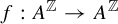
If
$f : A^{\mathbb {Z}} \to A^{\mathbb {Z}}$
 is a CA and
$\mu $
 is a shift-invariant measure on
$A^{\mathbb {Z}}$
 , then a given word w occurs in the
$\mu $
 -limit set
$\Omega _\mu (f)$
 if and only if
$\mu (f^{-n}(w))$
 does not converge to zero as n grows. In particular, if
$\mu $
 is the uniform Bernoulli measure, then w occurs in
$\Omega _\mu (f)$
 if and only if
$\limsup _n |f^{-n}(w)| / |A|^{|w|+2nr}> 0$
 . Generic limit sets of CAs have a combinatorial characterization as well.
Lemma 3.1. [Reference Törmä10]
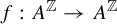
Let
$f : A^{\mathbb {Z}} \to A^{\mathbb {Z}}$
 be a CA and
$w \in A^*$
 . Then, w occurs in the generic limit set
 if and only if there exists a ‘seed’ word
$s \in A^*$
 and a position
$i \in \mathbb {Z}$
 such that for all
$u, v \in A^*$
 , there are infinitely many
$n \in \mathbb {N}$
 with
$f^n([u s v]_{i - |u|}) \cap [w]_0 \neq \emptyset $
 .
All three limit sets are non-empty subshifts of
$A^{\mathbb {Z}}$
 . The limit set contains the other two, but in general, neither of the generic limit set or the
$\mu $
 -limit set contains the other.
Lemma 3.2. [Reference Kůrka and Maass7, Reference Milnor9]
Let
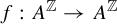
$f : A^{\mathbb {Z}} \to A^{\mathbb {Z}}$
 be a CA. Then,
 and
$\Omega _\mu (f) \subseteq \Omega (f)$
 .
4 Defect dynamics of rule 18
The local rule of ECA 18 is given in Table 1: the patterns 001 and 100 produce a 1 and all other patterns produce a 0. In the remainder of this paper, we denote this CA by
$f_{18}$
 , or just f when there is no danger of confusion. Figure 1 depicts a sample spacetime configuration of f. In this figure and in the following, time advances downward, a black square represents a 1 and a white square represent a 0. Hatched squares are undetermined symbols.
The local rule of ECA 18.

Table 1 Long description
The table consists of two rows and eight columns. The top row lists all possible three-digit binary neighborhood configurations, and the bottom row provides the resulting state for the central cell in the next time step.
* Column 1: 000 maps to 0
* Column 2: 001 maps to 1
* Column 3: 010 maps to 0
* Column 4: 011 maps to 0
* Column 5: 100 maps to 1
* Column 6: 101 maps to 0
* Column 7: 110 maps to 0
* Column 8: 111 maps to 0
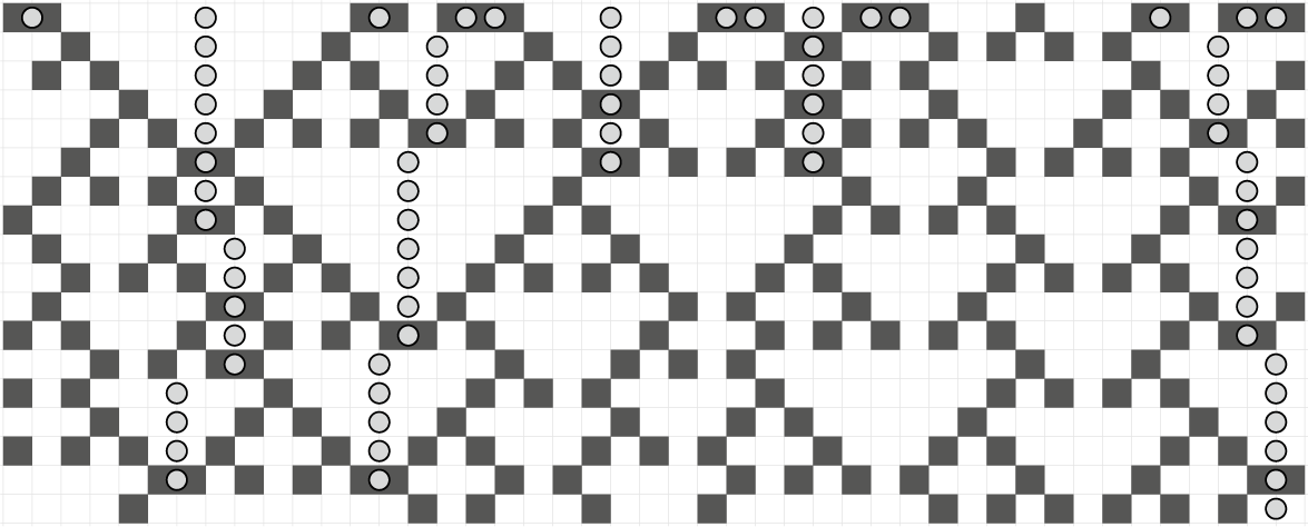
An example run of rule 18. The centre of each kink is marked with a circle.

Figure 1 Long description
A rectangular grid of 15 rows and approximately 50 columns. Dark gray squares represent active cells, while white squares are inactive. The top row serves as the initial state, containing several isolated dark squares and pairs of dark squares. As the rows progress downward, the dark squares propagate diagonally, creating triangular voids and intersecting paths. Small light gray circles are overlaid on specific cells to track the movement of kinks. These circles form vertical or slightly staggered columns, indicating the temporal path of these structural features. Some circular markers are clustered at the top where initial conditions are set, while others descend through the grid, often positioned at the apex or center of the evolving V-shaped patterns.
The dynamics of ECA rule 18 are a combination of several interacting processes. On regions where the gaps between 1-symbols have odd length, the dynamics is linear and well understood. A single gap of even length, called a kink, is persistent. Its movements are influenced by the linear part of the dynamics, but not vice versa: the linear dynamics commutes with a local operation that erases the kink. However, when two kinks collide, both are destroyed and the linear dynamics is perturbed.
Definition 4.1. Words of the form
$1 0^{2n} 1$
 with
$n \in \mathbb {N}$
 are called kinks. The left border of the kink is its leftmost
$1$
 -symbol.
Let
$x \in \{0,1\}^{\mathbb {Z}}$
 . We denote
$g_x(n) = \#\{-n \leq i \leq n \mid \text { there exists } k \in \mathbb {N}, x_{[i, i+2k+2]} = 1 0^{2k} 1\}$
 . If
$\lim _{n \rightarrow \infty } g_x(n) = m < \infty $
 , then we call m the number of kinks in x.
We call
$\Sigma \subseteq \{0,1\}^*$
 the set of words without kinks and
 the set of configurations without kinks.
Proposition 4.1. [Reference Jen5]
Let
$f_{90}$
 be the function associated with ECA rule
$90$
 :
$f_{90}(abc) = a \oplus c$
 for all
$abc \in \{0,1\}^3$
 , where
${\oplus }$
 is addition modulo 2, or the xor function. Then, for all kinkless words
$w \in \Sigma $
 , we have
$f_{18}(w) = f_{90}(w)$
 and for all kinkless configurations
 , we have
$f_{18}(x) = f_{90}(x)$
 .
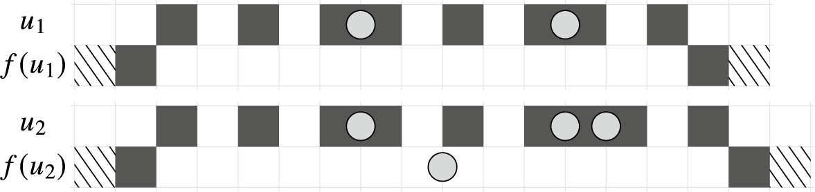
We now investigate the dynamics of kinks under rule 18. When n is even, the following lemma characterizes the preimages of kinks. See Figure 2 for an illustration with
$n = 13$
 and
$n = 14$
 .
Lemma 4.2. Let
$u \in \{0,1\}^*$
 be a word such that
$f(u) = 1 0^n 1$
 with
$n \in \mathbb {N}$
 . Then, either
$u = 1 0^{n+2} 1$
 or
$u = 00v00$
 for a word
$v \in \{0,1\}^*$
 that begins and ends in
$1$
 , does not contain occurrences of
$00$
 , and contains m occurrences of
$11$
 with
$m \not \equiv n \bmod 2$
 .
The word
$u_1$
 above contains an even number of kinks; hence,
$f(u_1)$
 is not a kink. The word
$u_2$
 below contains an odd number of kinks; hence,
$f(u_2)$
 is a kink.

Figure 2 Long description
The diagram consists of two horizontal rows of grid cells.
Top panel u sub 1 and f(u sub 1):
* The top row u sub 1 contains eight dark gray squares distributed across the grid. Two of these squares, located in the center-left and center-right, each contain a single light gray circle.
* The bottom row f(u sub 1) is mostly empty white cells, except for a dark gray square at the second and second-to-last positions. The far-left and far-right ends are marked with diagonal-striped blocks.
Bottom panel u sub 2 and f(u sub 2):
* The top row u sub 2 has a similar layout of dark gray squares. However, the center-left square contains one light gray circle, while the center-right square contains two light gray circles side-by-side.
* The bottom row f(u sub 2) contains a single light gray circle in a white cell at the center of the grid. Like the top panel, it features dark gray squares at the second and second-to-last positions and diagonal-striped blocks at both ends.
Proof. The word u both begins and ends with
$001$
 or
$100$
 , a priori independently of each other. If u begins with
$100$
 , then it must contain
$000$
 at positions
$1, 2, 3, \ldots $
 to avoid producing a
$1$
 in
$f(u)$
 and, finally, it ends with
$001$
 . Hence,
$u = 1 0^{n+2} 1$
 .
Suppose then that u begins with
$001$
 . We necessarily have
$n \geq 1$
 . Consider the smallest
$1 \leq i \leq n+2$
 such that u contains
$00$
 at position i; such an i exists since u ends with
$100$
 or
$001$
 . Then, u contains
$100$
 at
$i-1$
 , which means
$i = n+2$
 and u ends with
$100$
 . Hence,
$u = 001 w 100$
 , with
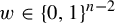
$w \in \{0,1\}^{n-2}$
 not containing occurrences of
$00$
 .
Consider the word
$1 w 1$
 as a concatenation of
$1$
 s and
$01$
 s, starting with a single
$1$
 . Each subsequent
$1$
 changes the parity of the length and adds a kink, while each
$01$
 keeps the parity of the length and adds no kinks. Hence, the number m of kinks in u satisfies
${m \not \equiv |1w1| = n \bmod 2}$
 .
In particular, Lemma 4.2 implies that new kinks cannot be created by rule 18.
Consider a kink
$K = 1 0^{2n} 1$
 occurring in an infinite configuration
$x \in \{0,1\}^{\mathbb {Z}}$
 . In
$f(x)$
 , K becomes
$1 0^{2n-2} 1$
 if
$n \geq 1$
 . If
$n = 0$
 (so that
$K = 11$
 ) and x is ‘typical’, K is contained in a subword of the form
$u = 0 0 1 w 1 0 0$
 , where w does not contain
$00$
 as a subword. Then,
$f_{18}(u) = 1 0^{|w|+2} 1$
 and by Lemma 4.2, this word is a kink if and only if the number of kinks in u is odd. Conversely, if the number of kinks in u is even, they are all destroyed. Hence, in ‘typical’ conditions, kinks can only be destroyed in pairs of
$11$
 s.
As an ‘atypical’ limiting case, consider a configuration
$x \in \{0,1\}^{\mathbb {Z}}$
 such that some infinite tail
$x_{[i, \infty )}$
 contains no occurrences of
$00$
 . Then,
$f(x)$
 contains the same number of kinks as
$f(y)$
 , where y is obtained from x by replacing the infinite tail by one of
$(01)^\infty $
 or
$(10)^\infty $
 in a way that does not introduce a new
$00$
 . Similarly, when
$f_{18}$
 is applied to finite words, their length decreases, so it is inevitable that all kinks are eventually destroyed as described above, or ‘fall off the edge of the word’ as in
${f(1100) = 01}$
 . The notion of stable words introduced in the following allows us to control this phenomenon.
The following definitions are inspired by [Reference Kůrka6].
Definition 4.2. Let
$w \in \{0,1\}^*$
 be a word that contains
$m \in \mathbb {N}$
 kinks. The finite kinkless extension
$\Sigma (w) \subseteq \{0,1\}^*$
 of w is the set of those words that contains w as a subword and contain exactly m kinks. The kinkless extension of w at position
$p \in \mathbb {Z}$
 is
 .
Definition 4.3. The (regular) language of left unstable words is
$(\epsilon + 0) (10)^* 11 (0+1)^*$
 and the language of right unstable words is
$(0+1)^* 11 (01)^* (\epsilon + 0)$
 . A word is unstable if it is left or right unstable. If a word is not unstable, it is stable. We denote by S the set of stable words.
In other words, a word is stable if it does not have a prefix of the form
$0 (10)^n 11$
 or
$(10)^n 11$
 or, symmetrically, a suffix of the form
$11 (01)^n 0$
 or
$11 (01)^n$
 for any
$n \geq 0$
 . For example,
$1010110001$
 is a left unstable word, while
$001010110001$
 is a stable word.
Intuitively, a word u is unstable if it contains an occurrence of the kink
$11$
 and can be extended into a word v such that the
$11$
 evolves into a kink K in
$f(v)$
 , but
$f(u)$
 does not fully contain K. For example,
$u = 1010110001$
 can be extended into
${v = 00u = 001010110001}$
 . The word
$f(v) = 1000000101$
 contains the kink
${K = 10000001}$
 , but
$f(u) = 00000101$
 is kinkless. We imagine the kink
$11$
 ‘falling off the edge’ as u evolves into
$f(u)$
 .
Kinkless extensions of stable words are also stable.
Proposition 4.3. Let
$v \in S$
 be a stable word. Then,
$\Sigma (v) \subseteq S$
 .
Proof. Let
$u v w \in \Sigma (v)$
 be a kinkless extension of v. Suppose for a contradiction that
$u v w$
 is left unstable (the right unstable case being symmetric), so it has
$(10)^n11$
 or
$0(10)^n11$
 as a prefix for some
$n \geq 0$
 . The kink
$11$
 occurs in v, so u is a prefix of
$(10)^n$
 or
$0(10)^n$
 . Hence, v has a prefix of the form
$0(10)^k 11$
 or
$(10)^k 11$
 for some
$k \geq 0$
 , that is, it is left unstable.
In stable words, kinks are necessarily erased in pairs. This is depicted in Figure 2. From this and the discussion preceding Definition 4.2, we infer the following proposition.
Proposition 4.4. Let
$w \in \{0,1\}^*$
 be a word that contains
$n \in \mathbb {N}$
 kinks. Then,
$f(w)$
 contains
$m \leq n$
 kinks. If
$w \in S$
 , then
$m \equiv n \bmod 2$
 .
Proof. We first match every kink in
$f(w)$
 to an odd number of kinks in w so that no kink of w is matched to two kinks of
$f(w)$
 . Namely, suppose
$f(w)$
 contains a kink
$K = 1 0^{2k} 1$
 whose left border is at position i and right border at position
$i+2k+1$
 . By Lemma 4.2, the subword
$w_{[i-1, i+2k+2]}$
 contains an odd number of kinks, which we match with K. The first claim follows from this matching.
Suppose then that w is stable. We prove the second claim by showing that in the above matching, the number of kinks of w not matched to a kink of
$f(w)$
 is even. Suppose w contains a kink
$K = 10^{2k}1$
 at position i. If
$k \geq 1$
 , then
$f(w)$
 contains
$10^{2(k-1)}1$
 at position i, which is matched to K.
Suppose thus
$k = 0$
 , so that
$K = 11$
 . Since w is stable, to the left of K, we must have an occurrence of
$00$
 ; let the rightmost one of those be at position
$i - p$
 . Then,
$p \geq 2$
 and w contains
$001$
 at position
$i-p$
 . Similarly, to the right of w, we find the leftmost occurrence of
$00$
 at
$i+q$
 for some
$q \geq 2$
 and then
$100$
 occurs at
$i+q-1$
 . Thus, w contains
$001 u 100$
 at position
$i-p$
 , where
$u \in \{0,1\}^{q+p-4}$
 has no occurrences of
$00$
 . Then,
$f(w)$
 contains
$L = 10^{q+p-2}1$
 at
$i-p$
 .
If
$q+p-2$
 is even, then L is a kink that is matched with K. If it is odd, then the length of u is also odd, so
$1u1$
 contains an even number of occurrences of the kink
$11$
 that are not matched to any kink of
$f(w)$
 . One of these is K and since K was arbitrary, it follows that every unmatched kink of w is part of such an even-sized collection.
The most important property of stable words is that they behave nicely with respect to kinkless extensions.
Proposition 4.5. Let
$w \in S$
 be a stable word. Then,
$f(\Sigma (w)) \subseteq \Sigma (f(w))$
 and
 for all
$p \in \mathbb {Z}$
 . If w is not of the form
$0^{\alpha } (10)^{n} 1^{\beta }$
 with
$\alpha , \beta \in \{0,1\}$
 and
$n \in \mathbb {N}$
 , then both inclusions are equalities.
In the case where w is of the form
$0^{\alpha } (10)^{n} 1^{\beta }$
 , the result holds ‘up to parity’: for each
${u = a f(w) b \in \Sigma (f(w))}$
 with
$u_i = 0$
 , whenever
$i \not \equiv |a| + \alpha \bmod 2$
 , we have
${u \in f(\Sigma (w))}$
 .
We also explain here the error in [Reference Kůrka6]. Page 15 of the article contains the claim that rule 18 is
$\Sigma _p$
 -permuting, which in our notation means
$f(\Sigma (w)) \subseteq \Sigma (f(w))$
 for every word
$w \in \{0,1\}^*$
 of length at least three. This may be false if w is not stable. For example, take
$w = 0011$
 , for which
$f(w) = 10$
 , and consider
$101 \in \Sigma (f(w))$
 .
Proof. Let
$a w b \in \Sigma (w)$
 . We claim that
$f(a w b) \in \Sigma (f(w))$
 , that is, all kinks of
$f(a w b)$
 are contained in
$f(w)$
 . Consider any subword u of
$a w b$
 such that
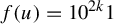
$f(u) = 1 0^{2k} 1$
 is a kink. By Lemma 4.2, there are two possibilities.
-
(1) $u = 1 0^{2k+2} 1$
is itself a kink and wider than
$f(u)$
. If
$f(u)$
is not contained in
$f(w)$
, then u is not contained in w, which contradicts
$a w b \in \Sigma (w)$
. -
(2) $u = 0 0 v 0 0$
for some word v that begins and ends with
$1$
, does not contain an occurrence of
$0 0$
, and contains at least one occurrence of
$1 1$
(which must be within w). If
$f(u)$
is not contained in
$f(w)$
, then u is not contained in w, which contradicts the stability of w.



Suppose then that w is not of the form
$0^{\alpha } (10)^{n} 1^{\beta }$
 and let
$a f(w) b \in \Sigma (f(w))$
 . We claim that some
$c w d \in \Sigma (w)$
 satisfies
$f(c w d) = a f(w) b$
 . It suffices to consider
$|a| = 1$
 and
$|b| = 0$
 ; the general result follows by iteration and symmetry. There are a few cases.
-
(1) If $a = 0$
and w does not begin with
$0 1$
, we can choose
$c = 0$
. -
(2) If $a = 0$
and w begins with
$0 1$
, we can choose
$c = 1$
. -
(3) If $a = 1$
and w begins with
$0 0$
, then the assumption
$a f(w) b \in \Sigma (f(w))$
implies that either
$w = 0^{|w|}$
or w begins with
$0^{2n+1} 1$
for some
$n \geq 1$
. We can then choose
$c = 1$
. -
(4) If $a = 1$
and w begins with
$0 1$
, we can choose
$c = 0$
. -
(5) Suppose $a = 1$
and w begins with
$1$
. By stability and the assumption that w is not of the form
$0^{\alpha } (10)^{n} 1^{\beta }$
, it must begin with
$1 (0 1)^n 0 0$
for some
$n \in \mathbb {N}$
. However, then,
$a f(w)$
begins with
$1 0^{2n} 1$
, which contradicts
$a f(w) b \in \Sigma (f(w))$
. Hence, this case is impossible.






The claims about  follow easily.
From this and Proposition 4.1, we get the following corollary.
Corollary 4.6. Let
$w \in S$
 be a stable word of length at least 2 and not of the form
$0^\alpha (10)^n 1^\beta $
 for
$\alpha , \beta \in \{0,1\}$
 . For each
$u = a f(w) b \in \Sigma (f(w))$
 , there exist unique
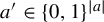
${a' \in \{0,1\}^{|a|}}$
 and
$b' \in \{0,1\}^{|b|}$
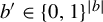 with
$f(a' w b') = u$
 .
Corollary 4.7. We have
$f(\Sigma ) = \Sigma $
 and
 .
Finally, we make use of the following result to bring down the number of kinks in an initial configuration.
Theorem 4.8. [Reference Jen5, Proposition 5]
Let
$x \in \{0,1\}^{\mathbb {Z}}$
 be a configuration with a finite number of
$1$
 -symbols. Then, for all large enough
$n \in \mathbb {N}$
 , the configuration
$f^n(x)$
 contains at most one kink. Moreover, this
$f^n(x)$
 is kinkless if and only if x has an even number of kinks.
Corollary 4.9. Let
$w \in \{0,1\}^*$
 be a word with an even number of kinks. Then, there exists
$n \in \mathbb {N}$
 such that
$f^n(\Sigma (0^n \cdot w \cdot 0^n)) \subseteq \Sigma $
 and
 for all
${p \in \mathbb {Z}}$
 .
Proof. Let
$x \in \{0,1\}^{\mathbb {Z}}$
 be the configuration with w at position zero and
$0$
 -symbols everywhere else. By Theorem 4.8, for some
$n \geq 2$
 , the configuration
$f^n(x)$
 is kinkless. The word
$u = f^n(0^n \cdot w \cdot 0^n) \in \Sigma $
 occurs in
$f^n(x)$
 at position zero. Since
$0^n \cdot w \cdot 0^n$
 is stable, by Proposition 4.5, we have
$f^n(\Sigma (0^n \cdot w \cdot 0^n)) \subseteq \Sigma (f^n(0^n \cdot w \cdot 0^n)) = \Sigma (u) \subseteq \Sigma $
 . The second claim is similar.
5 The generic limit set of rule 18
In this section, we characterize the set of words with at most two kinks that occur in the generic limit set of rule 18. In principle, the cases of zero or one kink (Theorems 5.1 and 5.5) are subsumed by the case of two kinks (Theorem 5.9), since all words of at most one kink occur as subwords of two-kink words in the generic limit set. We present proofs for these cases as well to showcase our techniques in a simpler context. In the case of zero kinks, the idea is simple: use Theorem 4.8 to erase all existing kinks, then use the permutivity of
$f_{18}$
 on kinkless configurations to produce an arbitrary kinkless word.
5.1 Kinkless words
We begin with the easiest case of kinkless words.
Theorem 5.1. Every word with no kinks occurs in  .
Proof. Let
$w \in \Sigma $
 be a kinkless word. We consider the seed
$\epsilon $
 at position
$i = 0$
 . Let
$q_1, q_2 \in \{0,1\}^*$
 be arbitrary words. Our goal is to show that
$f^k([q_1 q_2]_{-|q_1|})$
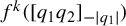 intersects
$[w]_0$
 for infinitely many k.
There exists a word
$r \in \{0,1\}^*$
 such that
$q_1 q_2 r$
 contains an even number of kinks. According to Corollary 4.9, there exists
$n_0 \in \mathbb {N}$
 such that for all
$n \geq n_0$
 and all configurations
 , the image
$f^n(x)$
 contains no kinks. In the following, we call
$u = 0^{2n+2} \cdot q_1 q_2 r \cdot 0^{2n+2}$
 .
For each
$m \leq n$
 , the word
$f^m(u)$
 begins and ends in
$0 0$
 , so it is stable and not of the form
$0^\alpha (1 0)^k 1^\beta $
 for
$\alpha , \beta \in \{0,1\}$
 and
$k \in \mathbb {N}$
 . By iterating Proposition 4.5, we have

The word
$f^n(u)$
 and, hence, each configuration in
 contain no kinks. Suppose that
$|q_1|, |q_2 r|$
 are both even, and all
$1$
 -symbols in
$f^n(u)$
 and w occur in even positions (the other cases are handled similarly). Then, all
$1$
 -symbols in
$f^{|q_2r|+n+2}(u)$
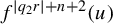 also occur at even positions, so
$f^{|q_2r|+n+2}(u) w$
 contains no kinks:
$f^{|q_2r|+n+2}(u) w \in \Sigma (f^{|q_2r|+n+2}(u))$
 . Again by iterating Proposition 4.5 (and the remark following it), we obtain
 . Hence, as long as
$q_1$
 and
$q_2$
 are long enough (as we can choose them to be), there exists a word v of length
$|w|$
 such that
$f^n(u) v$
 contains no kinks and
$f^{|q_2 r|+n+2}(f^n(u) v)$
 ends in w. In total, we have

which shows that
$[w]_0$
 intersects
$f^k([q_1 q_2]_{-|q_1|})$
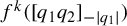 for some
$k \geq n$
 . Since n can be arbitrarily large, Lemma 3.1 gives that w occurs in
 .
5.2 Words with one kink
In this section, we show that all words with exactly one kink occur in the generic limit set of rule 18. The idea is to again erase all existing kinks except one, then direct it to a specific position and use permutivity to control the kinkless region around it.
Lemma 5.2. Let w be a one-kink word. Then, there exists
$n \in \mathbb {N}$
 such that
$f^n(w)$
 is a left unstable or right unstable word.
Proof. We proceed by induction on
$|w|$
 . If
$|w| = 2$
 or
$|w| = 3$
 , then w must contain
$11$
 as a prefix or suffix, so it is already unstable. Otherwise, if w is stable, it is easy to see that
$f(w)$
 is also a one-kink word. By the induction hypothesis, there exists some
$n'$
 such that
$f^{n'}(f(w))$
 is left or right unstable. Hence, the property is true for
$n = n'+1$
 .
Definition 5.1. A left kink word is a finite word that begins with a kink and contains no other kinks. The set of left kink words is denoted
$L \subset \{0,1\}^*$
 .
The following lemma tells us that
$11$
 can be produced from any word in L. As any one-kink word can be produced in one step from
$11$
 , it follows from this lemma that any one-kink word can be produced from any word of L.
Lemma 5.3. For all left kink words
$w \in L$
 , there exists
$n \in \mathbb {N}$
 such that
$\Sigma (11) \subseteq f^n(\Sigma (w))$
 .
Proof. We prove the result by induction on the size of w. There are a few cases.
-
(1) If $|w| = 2$
, then
$w = 11$
and the result is immediate. Otherwise,
$|w| \geq 3$
and we suppose that the property holds for all shorter words. -
(2) If w begins with $10^{2k}1$
for some
$k> 0$
, then
$f(w) \in L$
and
$|f(w)| < |w|$
. Then,
$\Sigma (11) \subseteq f^n(\Sigma (f(w)))$
for some
$n \in \mathbb {N}$
by the induction hypothesis and since
${w \in S}$
, Proposition 4.5 gives
$f^n(\Sigma (f(w))) \subseteq f^{n+1}(\Sigma (w))$
. -
(3) If w is of the form $11 (01)^k 0$
for some
$k \in \mathbb {N}$
, then we consider
$w' = 00 w 0 \in \Sigma (w)$
. We have
$f^{k+2}(w') = 11$
and
$\Sigma (f^{k+2}(w')) = f^{k+2}(\Sigma (w'))$
by Proposition 4.5, and we can choose
$n = k+2$
. -
(4) If w is of the form $11 (01)^k$
with
$k \geq 1$
, then we consider
$w' = 00 w 00 \in \Sigma (w)$
and conclude as in the previous case. -
(5) If w is of the form $11 (01)^k 00 u$
for some word u and
$k \in \mathbb {N}$
, then we consider
${w' = 00 w}$
. We have
$f(w') = 1 0^{2(k+1)} 1 v$
for some word v. Then, we treat
$f(w')$
as in case (2) and conclude.










These cases are exhaustive. Namely, we know w begins with
$10^{2k}1$
 . If
$k \geq 1$
 , we are in case (2). If not, then either
$w = 11$
 (case (1)) or w continues with alternating
$0$
 s and
$1$
 s until the first occurrence of
$00$
 (case (5)), if any, as it does not contain another
$11$
 . Cases (3) and (4) correspond to w containing no
$00$
 , so the alternating
$0$
 s and
$1$
 s continue until the end of w.
The following lemma is a direct consequence of the previous one; it shows that any one-kink word can be produced at any position from any other one-kink word at position zero.
Lemma 5.4. Let w and
$w'$
 be two words containing one kink. Then, for all
$i \in \mathbb {Z}$
 , there exists
$n \in \mathbb {N}$
 such that
 .
The idea is to let the kink of w evolve into a
$11$
 whose context we can freely choose. Then, we can easily produce another
$11$
 at any desired position at a later time step. This
$11$
 can then be transformed into
$w'$
 in a single step.
Proof. Let
$k \in \mathbb {N}$
 be the smallest number for which
$f^k(w)$
 is unstable. We may assume that it is left unstable. By Proposition 4.4,
$f^k(w)$
 contains one kink, which must be
$11$
 . Then,
$f(00 \cdot f^k(w))$
 is a left kink word.
According to Lemma 5.3, there exists
$m \in \mathbb {N}$
 such that
$\Sigma (11) \subseteq f^m(\Sigma (f(00\cdot f^k(w))))$
 and Proposition 4.5 gives
$f^m(\Sigma (f(00\cdot f^k(w)))) \subseteq f^{k + m+1}(\Sigma (w))$
 . We can deduce that there exists a position
$p \in \mathbb {Z}$
 such that
 .
Since
$w'$
 is a one-kink word, it has the form
$a 1 0^{2\ell } 1 b$
 for some
$a, b \in \{0,1\}^*$
 and
$\ell \in \mathbb {N}$
 . Suppose that
$p \leq |a|$
 , the other case being similar. Consider
$w_0 = 0011 (01)^{|a|-p+1}00$
 . We have
$f^{|a|-p + 3}(w_0) = 11$
 and all the intermediate steps are stable; hence, Proposition 4.5 gives
 .
The word
$u = 0011 (01)^{\ell } 00$
 is stable and
$f(u) = 1 0^{2\ell } 1$
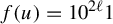 , so we obtain
 by Proposition 4.5. Putting everything together, we have
 , as claimed.
Theorem 5.5. Every one-kink word occurs in  .
Proof. Let
$w \in \{0,1\}^*$
 be a one-kink word. We consider the seed
$\epsilon $
 . Let
$q_1, q_2 \in \{0,1\}^*$
 be words, and choose
$r \in \{0,1\}^*$
 and
$n_0 \leq n \in \mathbb {N}$
 as in the proof of Theorem 5.1, except that
$q_1 \cdot q_2 \cdot r$
 should contain an odd number of kinks and every configuration in
 should contain a single kink. Call
$u = 0^{2n+2} \cdot q_1 \cdot \epsilon \cdot q_2 \cdot r \cdot 0^{2n+2}$
 .
For all
$m \leq n$
 ,
$f^m(u)$
 is a stable one-kink word, so that
 . According to Lemma 5.4, there exists
$k \in \mathbb {N}$
 such that
 . This means that
$[w]$
 intersects
$f^{n+k}([q_1 q_2]_{-|q_1|})$
 . Since n can be arbitrarily large, Lemma 3.1 implies that w occurs in
 .
5.3 Words with two kinks
In this section, we determine the set P of words with exactly two kinks that appear in the generic limit set of rule
$18$
 . The idea is to erase all existing kinks except two, then bring the two kinks close to each other to produce the word
$1101001$
 and then to show that all words of P can be produced from a two-kink configuration that contains
$1101001$
 at any position.
Denote the reversal of a word
$w \in \{0,1\}^*$
 by
$w^R$
 . For a set
$L \subseteq \{0,1\}^*$
 , we denote
$L^R = \{w^R \mid w \in L\}$
 .
Definition 5.2. We call
$B \subset \{0,1\}^*$
 the set of two-kink words that begin with
$11$
 , end with a kink (which can overlap with the prefix
$11$
 ) and are not of the form
$11 \cdot (01)^k \cdot 1$
 for
$k \in \mathbb {N}$
 .
This definition is useful as B is a set of words containing two kinks that we can prevent from colliding. The following lemma states that we can direct the two kinks of a word of B so that they can be brought close and produce the word
$1101001$
 .
Lemma 5.6. Let
$w \in B \cup B^R$
 be a word. Then, there exists
$n \in \mathbb {N}$
 such that
$\Sigma (1101001) \subseteq f^n(\Sigma (w))$
 .
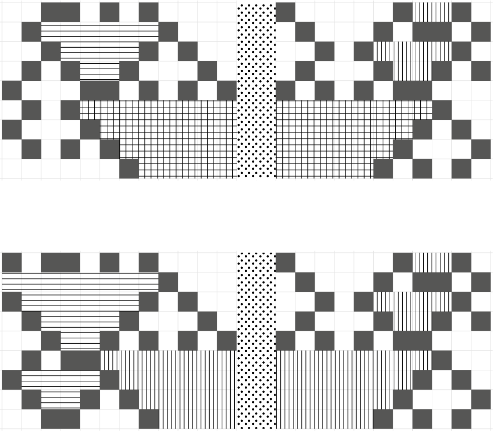
The proof of this lemma contains many different cases; however, the cases are quite natural and the proof of each case is easy. The main idea of the proof is that by forbidding the kinks to move away from each other, it is possible to bring them eventually closer. When the two kinks are on the verge of colliding, it is possible to avoid the collision and to instead make them closer to each other as illustrated in Figure 3.
Proof. First, we show that it suffices to prove the result for
$w \in B$
 . Namely, then for
$w \in B^R$
 , we have
$\Sigma (1001011) \subseteq f^n(\Sigma (w))$
 for some
$n \in \mathbb {N}$
 by symmetry and a direct computation shows that
$f^3(10 \cdot 1001011 \cdot 0100) = 1101001$
 , so that
$\Sigma (1101001) \subseteq f^{n+3}(\Sigma (w))$
 .
Two kinks collide and annihilate each other, but it is possible to avoid collision by making the leftmost kink longer.

Figure 3 Long description
The diagram consists of two horizontal panels on a white grid.
Top Panel:
On the left, a region filled with horizontal lines is bounded by dark gray pixels. This region moves toward the center. On the right, a region with vertical lines is similarly bounded. In the center, a vertical column with a dotted pattern acts as a divider. The horizontal and vertical patterned regions meet at this central column, forming a large cross-hatched area where they overlap, indicating a collision.
Bottom Panel:
This panel shows a variation of the interaction. The leftmost region with horizontal lines is elongated vertically compared to the top panel. Because of this structural change, the patterned regions on the left and right do not merge into a single cross-hatched block at the center. Instead, they remain distinct or separated by the central dotted column and dark gray pixel boundaries, demonstrating how collision is avoided by altering the length of the leftmost kink.
Let then
$w \in B$
 be arbitrary. We proceed by induction on the length of w.
Case 0:
$|w| \leq 7$
 . There are only a few possibilities for w. If
$w = 1101001$
 , the result is immediate. If
$w = 11001$
 , then
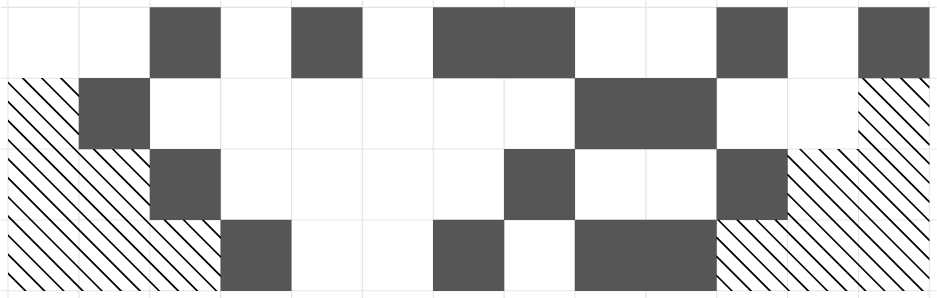
$\Sigma (1001011) \subseteq f^3(\Sigma (w))$
 as shown in Figure 4 and
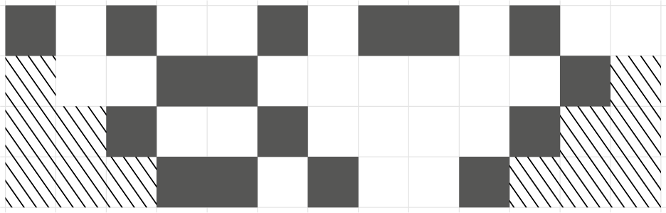
$\Sigma (1101001) \subseteq f^3(\Sigma (1001011))$
 as shown in Figure 5; hence,
$\Sigma (1101001) \subseteq f^6(\Sigma (w))$
 . If
$w = 1100001$
 , then
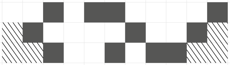
$\Sigma (1101001) \subseteq f^2(\Sigma (1001011)) \subseteq f^5(\Sigma (w))$
 as shown in Figure 6. If
$w = 1100011$
 , then
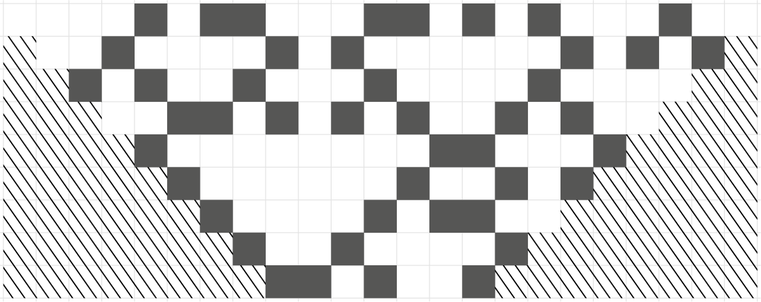
$\Sigma (1101001) \subseteq f^8(\Sigma (000010 \cdot w \cdot 0101000100)) \subseteq f^8(\Sigma (w))$
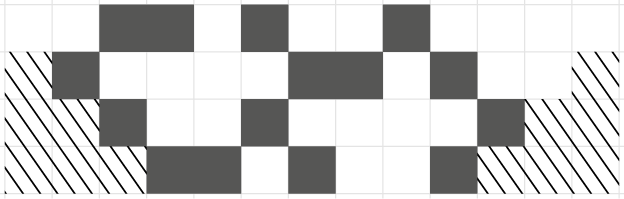
 as shown in Figure 7.
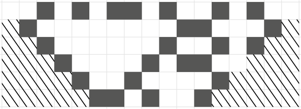
We can see here that
$w = 0010101100101$
 is stable,
$f(w)$
 and
$f^2(w)$
 are stable, and
$f^3(w) = 1001011$
 . We can deduce that
$\Sigma (1001011) = f^3(\Sigma (w)) \subseteq f^3(\Sigma (1001011))$
 .

We can see here that
$w = 1010010110100$
 is stable,
$f(w)$
 and
$f^2(w)$
 are stable, and
$f^3(w) = 1101001$
 . We can deduce that
$\Sigma (1101001) = f^3(\Sigma (w)) \subseteq f^3(\Sigma (1001011))$
 .

We can see here that
$w = 00101100001$
 is stable,
$f(w)$
 is stable and
$f^2(w) = 1001011$
 . We can deduce that
$\Sigma (1101001) \subseteq f^2(\Sigma (1001011)) = f^5(\Sigma (w)) \subseteq f^5(\Sigma (1100001))$
 .

We can see here that
$w = 00001011000110101000100$
 is stable,
$f(w), f^2(w), \ldots , f^7(w)$
 are stable and
$f^8(w) = 1101001$
 . We can deduce that
$\Sigma (1101001) = f^8(\Sigma (w)) \subseteq f^8(\Sigma (1100011))$
 .

Figure 7 Long description
A grid of 23 columns and 9 rows. Dark squares represent state 1 and white squares represent state 0.
Row 1: Dark squares at columns 5, 7, 8, 12, 13, 15, 17, 21.
Row 2: Dark squares at columns 4, 9, 11, 18, 20, 22. Diagonal hatching begins on the far left and right edges.
Row 3: Dark squares at columns 3, 8, 12, 17, 21.
Row 4: Dark squares at columns 6, 7, 9, 11, 13, 16, 18.
Row 5: Dark squares at columns 5, 14, 15, 19.
Row 6: Dark squares at columns 6, 13, 16, 18.
Row 7: Dark squares at columns 7, 12, 14, 15.
Row 8: Dark squares at columns 8, 11, 16.
Row 9: Dark squares at columns 9, 10, 12, 15.
The diagonal hatching on the left and right sides expands inward as the rows progress downward, creating a V-shaped active area for the automaton. The pattern of dark squares within this V-shape represents the evolution of the string w through successive applications of the function f.
For the rest of the proof, we suppose
$|w|> 7$
 and all shorter words of
$B \cup B^R$
 satisfy the claim.
Case 1:
$w = 11 0^{2k} 1$
 for some
$k \in \mathbb {N}$
 . Then,
$k \geq 3$
 . We consider
$w_0 = 00 \cdot w$
 . Then,
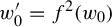
$f^2(w_0) = 1101 0^{2(k-2)} 1$
 . Evidently,
$f^2(w_0) \in B$
 ,
$|f^2(w_0)| < |w|$
 and
$\Sigma (f^2(w_0)) \subseteq f^2(\Sigma (w))$
 , so we can conclude by induction.
Case 2:
$w = 1101 0^{2k} 1$
 for some
$k \in \mathbb {N}$
 . Then,
$k \geq 2$
 . We consider
$w_0 = 00 \cdot w$
 . If
$k = 2$
 , then
$f^2(w_0) = 1001011$
 , which we treated in Case 0. If
$k = 3$
 , then
$f^3(w_0) = 1100011$
 , which we already treated as well. If
$k \geq 4$
 , then
$f^3(w_0) = 110001 0^{2(k-3)} 1 \in B$
 and
$|f^3(w_0)| < |w|$
 . We can then conclude by induction.
Case 3:
$w = 11 (01)^k 0^{2\ell } 1$
 for some
$k, \ell \geq 1$
 . We consider
$w_0 = 00 \cdot w$
 . Then,
$f(w_0) = 1 0^{2(k+1)} 1 0^{2(\ell -1)} 1$
 , so that for
$m = \min (k+1, \ell -1)$
 , the word
$w' = f^{m+1}(w_0)$
 begins and/or ends with
$11$
 . If
$\ell = 1$
 , then
$|w'| = |w|$
 and we can handle
$w'$
 as in Case 1. Otherwise,
$|w'| < |w|$
 . If
$w' \in B \cup B^R$
 , then we can conclude by induction. If
$w' \notin B \cup B^R$
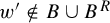 , then
$\ell = k+2$
 and
$w' = 11 (01)^{2(k+1)} 1$
 . Then, we instead consider
$w_1 = 0010 \cdot w$
 , for which
$f^{k+1}(w_1) = 1001 \cdot u \cdot 11$
 for some word u of length
$2(k+1)$
 . This word is in
$B^R$
 and is shorter than w, so we conclude by induction.
If we are not in the above cases, then the gap between the two kinks is longer than one cell and contains an occurrence of
$00$
 . Considering the leftmost occurrence of
$00$
 , we see that there exist
$k, \ell \in \mathbb {N}$
 and a word u such that
$w = 11 (01)^k 00 \cdot u \cdot 1 0^{2\ell } 1$
 . The remaining cases constrain the values of k and
$\ell $
 .
Case 4:
$\ell \geq 2$
 . We again consider
$w_0 = 00 \cdot w$
 and split into subcases depending on the value of k. If
$k = 0$
 , we consider
$w_0' = f^2(w_0)$
 , which begins with
$11$
 and ends with
$10^{2(\ell -2)}1$
 . If
$w_0' \in B$
 , we can conclude by induction as
$|w_0'| < |w|$
 . Otherwise,
$\ell = 2$
 and
$w_0' = 11 (01)^{(|w|-6)/2} 011$
 . Then, we instead consider
$v_0 = 0010 \cdot w \cdot 00$
 , which satisfies
$f^3(v_0) = 11 (00)^{(|w|-3)/6} \cdot 1$
 . We can now conclude using Case 1, as
$|f^3(v_0)| = |w|$
 .
If
$0 < k < \ell -2$
 , then
$f^{k+2}(w_0) \in B$
 and
$|w_0| < |w|$
 , so we can conclude using induction.
If
$k = \ell -2$
 , then consider
$w' = f^\ell (w_0)$
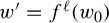 . If
$w' \in B$
 , we have
$|w'| < |w|$
 and we conclude by induction. If
$w' \notin B$
 , we instead consider
$w_1 = 0010 \cdot w$
 . Then,
$f^{\ell +1}(w_1) \in B^R$
 and
$|f^{\ell +1}(w_1)| < |w|$
 , so we conclude using induction.
If
$k> \ell -2$
 , then
$f^\ell (w_0) \in B^R$
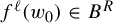 and
$|f^\ell (w_0)| < |w|$
 . We conclude by induction.
Case 5:
$\ell \leq 1$
 and
$k \geq 1$
 . If
$\ell = 0$
 , then we consider
$w_0 = 00 \cdot w \cdot 00$
 . Now,
$f(w_0)$
 begins with
$1 0^{2(k+2)} 1$
 and ends with
$1 0^{2 m} 1$
 for some
$m \geq 1$
 . We proceed as in Case 3, using
$w_1 = 0010 \cdot w \cdot 00$
 instead of
$w_0$
 as needed. If
$\ell = 1$
 , then
$f(w_0)$
 is in
$B^R$
 , has the same length as w and belongs to Case 3, which we already solved.
Case 6:
$\ell = 1$
 and
$k = 0$
 . We consider
$w_0 = 00 \cdot w$
 and denote
$w_0' = f(w_0)^R$
 , which begins with
$11$
 and ends with
$1 001$
 . If
$w_0'$
 belongs to one of the already solved Cases 0–5, then we are done. Otherwise,
$w_0' \in B$
 belongs to Case 6. Then, we repeat this process: for each
$i \in \mathbb {N}$
 , as long as
$w_i'$
 belongs to Case 6, define
$w_{i+1} = 00 \cdot w_i'$
 and
$w_{i+1}' = f(w_{i+1})^R = 11 \cdot u_{i+1} \cdot 1001$
 . Suppose that we reach
$w_{|w|}$
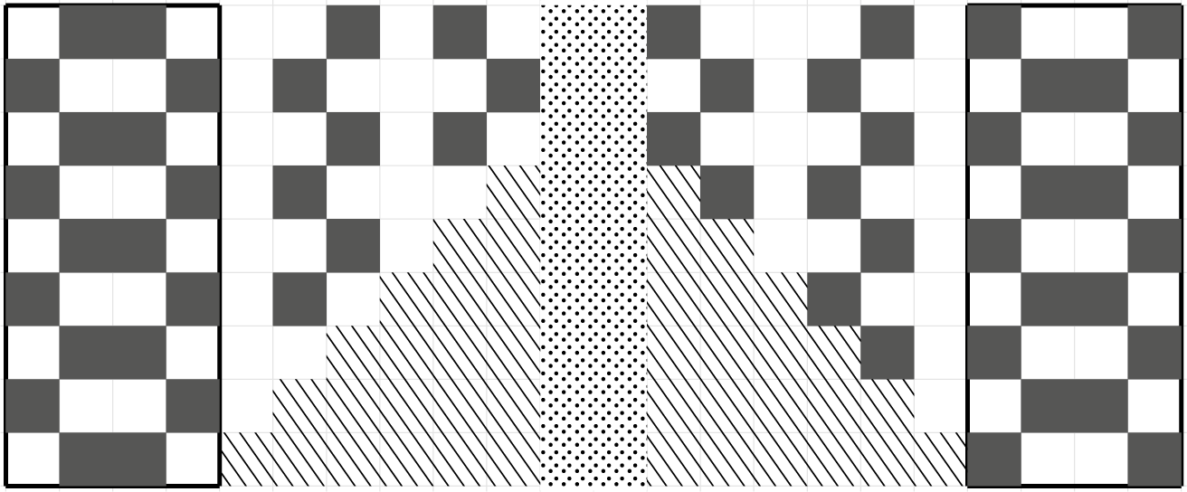
 this way. We can now go backward in time as shown in Figure 8: for each
$j \geq 0$
 , the length-j prefix and suffix of
$u_{|w|-j}$
 are determined locally. In the end, we determine that
$w = 1 \cdot (100010)^{(|w| - 5)/6} \cdot 1001$
 .
At each step of the backward computation, we force the four left and four right symbols to be either
$0110$
 or
$1001$
 , this in turn fixes the neighbours symbols to some value. After enough steps, the whole word is forced.

Figure 8 Long description
The diagram consists of a horizontal grid of square cells.
1. Left Boundary: A vertical rectangle four cells wide is outlined in a thick black border. It contains a repeating checkerboard pattern of dark gray and white squares representing the binary sequence 0 1 1 0 or 1 0 0 1.
2. Left Transition Zone: To the right of the boundary, dark gray squares form a descending staircase pattern from top-left to bottom-right. Below this diagonal, cells are filled with a diagonal hatching pattern that grows wider toward the center.
3. Center Column: A single vertical column of cells is filled with a dense stippled or dotted pattern, acting as a central axis.
4. Right Transition Zone: Mirroring the left, dark gray squares form an ascending staircase pattern from top-right to bottom-left. A diagonal hatching pattern fills the area below these squares, narrowing toward the right boundary.
5. Right Boundary: A vertical rectangle four cells wide is outlined in a thick black border, containing the same repeating checkerboard pattern as the left boundary.
We now consider
$v_0 = 0010 \cdot w \cdot 01$
 instead of
$w_0$
 . Then,
$v_0' = f^3(v_0) = 110 \cdot (101000)^{(|w|-5)/6} \cdot 11$
 and
$v_1' = f^4(00 \cdot v_0' \cdot 0001)$
 verifies
$v_1' \in B$
 and
$|v_1'| < |w|$
 . We can then conclude using induction.
Case 7:
$\ell = k = 0$
 . We consider
$w_0 = 00 \cdot w \cdot 00$
 and
$w_0' = f^2(w_0)$
 . If
$w_0'$
 belongs to one of the already solved cases, then since
$|w_0'| = |w|$
 , we are done. If
$w_0'$
 belongs to Case 7, we again repeat the process: for each
$i \in \mathbb {N}$
 , as long as
$w_i'$
 belongs to Case 7, define
$w_{i+1} = 00 \cdot w_i' \cdot 00$
 and
$w_{i+1}' = f^2(w_{i+1}) = 11 \cdot u_{i+1} \cdot 11$
 . In the same way as in Case 6, if we reach
$w_{|w|}$
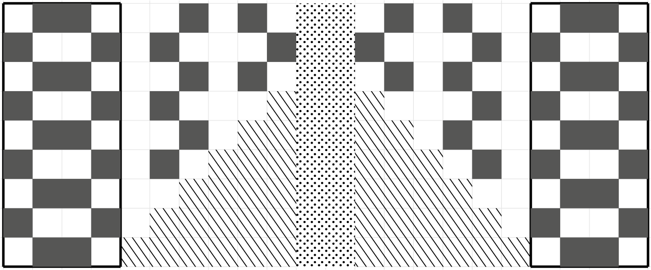
 in this way, we go backward in time as shown in Figure 9 to fully determine that
$w = 11000 \cdot (101000)^{(|w| - 7)/6} \cdot 11$
 .
In the same way as in Figure 8, after enough steps of backward computation, the whole word is forced.

Figure 9 Long description
The diagram is composed of a grid with several distinct vertical sections.
1. Far Left and Far Right: Two identical columns enclosed in thick black borders. Each contains a vertical checkerboard pattern of dark gray and white squares.
2. Inner Left and Inner Right: Moving inward from the borders, there are sections of dark gray squares arranged in a staggered, diagonal descending pattern.
3. Lower Center-Left and Center-Right: Below the staggered gray squares, two triangular regions are filled with diagonal hatching lines. These regions slope upward toward the center.
4. Center Column: A single vertical column at the exact center of the grid is filled with a dense stippled or dotted pattern, acting as the axis of symmetry for the entire diagram.
We now consider
$v_0 \kern1.5pt{=}\kern1.5pt 0010 \cdot w \cdot 0001$
 . Then,
$v_0' \kern1.5pt{=}\kern1.5pt f^3(v_0) \kern1.5pt{=}\kern1.5pt 110101 \cdot (000101)^{(|w|-7)/6} \cdot 001$
 and
$v_1' = f^4(00 \cdot v_0' \cdot 0100) = 1100 \cdot (000101)^{(|w|-7)/6} \cdot 001$
 . We are now in Case 6, which was already solved, with
$|w| = |v_1'|$
 .
Finally, we explain why the cases are exhaustive. Since
$w \in B$
 , it begins with
$11$
 , ends with a kink
$1 0^{2\ell } 1$
 and contains no other kinks. If the two kinks overlap, we are in Case 1. If they are separated by a single
$0$
 , we are in Case 2. If they are separated by a longer alternating sequence of
$0$
 s and
$1$
 s, then by the definition of B, we must have
$\ell \geq 1$
 , so we are in Case 3. Otherwise, as explained after Case 3, we have
$w = 11(01)^k00 \cdot u \cdot 10^{2\ell }1$
 for some word u, and Cases 4–7 cover all values of k and
$\ell $
 . This finishes the proof.
Lemma 5.7. Let
$i, j \in \mathbb {Z}^2$
 be two positions, then there exists
$n \in \mathbb {N}$
 such that
 .
Proof. We proceed by induction on
$|i-j|$
 . If
$i = j$
 , we can choose
$n = 0$
 . If
$i < j$
 , then
 as shown in Figure 10 and we can conclude using induction. If
$i> j$
 , then
 as shown in Figure 11 and we can conclude using induction.
Moving a
$1101001$
 one step to the left.

Moving a
$1101001$
 one step to the right.

The following definition provides us with a set P of words that can be produced from
$1101001$
 and, as we show later, these words constitute exactly the words of the generic limit set that have two kinks.
Definition 5.3. Let w be a word that contains exactly two kinks. We call
$b(w)$
 the smallest subword of w that contains two kinks. If
$b(w) = 1 0^{2k} 1 \cdot u \cdot 1 0^{2\ell } 1$
 for some
$k, \ell \in \mathbb {N}$
 and
$u \in \{0,1\}^*$
 , then we call
$\delta (w) = u$
 . If
$b(w)$
 is of the form
$10^{2k} 1 0^{2\ell } 1$
 , then we call
$\delta (w) = \epsilon $
 .
Definition 5.4. We define
$P \subset \{0,1\}^*$
 as the set of those two-kink words w that satisfy all of the following:
-
• $b(w) \neq 111$
; -
• if $b(w) = 11 v 11$
, then v contains an even number of
$1$
s; -
• for all $k \in \mathbb {N}$
,
$b(w) \neq 1 (100010)^k 1001$
and
$b(w) \neq 1001 (010001)^k 1$
.






Our goal is to prove that P coincides with the set of two-kink words of the generic limit set of f. The first two conditions are necessary, since the words
$111$
 and
$11v11$
 with v containing an odd number of
$1$
 s have no preimages under f. Namely, the only preimage of
$11$
 is
$1001$
 , which already forbids
$111$
 . However, one can prove by induction on the length of w that if w contains an even number of
$1$
 s, then all preimages of
$11w$
 end in
$01$
 ,
$10$
 or
$11$
 and, otherwise, they all end in
$00$
 . Then,
$11v11$
 has no preimage, as it would have to end in both
$1001$
 and
$00ab$
 for some
$a, b \in \{0,1\}$
 . Similarly, every two-kink word
$11w11$
 where w contains an even number of
$1$
 s has a unique two-kink preimage (and possibly other preimages with more kinks): if
$w = 0^{2n_0-1} 1 0^{2n_1-1} 1 \cdots 1 0^{2n_{2k}-1}$
 , that preimage is
$100 (10)^{n_0} 0^{2n_1} (10)^{n_2} 0^{2n_3} \cdots (10)^{n_{2k}} 01$
 .
We now proceed backwards in time and try to find for every word in P a parent that contains
$1101001$
 . Just as in Lemma 5.6, the proof is a combination of an induction and a case analysis. There are quite a few cases, but none of them is very difficult. The main idea is that we are first trying to close the gap between the two kinks in the word and then shorten the kinks.
Lemma 5.8. Let
$w \in P$
 . Then, there exists
$n \in \mathbb {N}$
 and a position
$p \in \mathbb {Z}$
 such that
 .
Proof. We first handle the ‘trivial’ cases.
Case 0: w contains
$1101001$
 or its reversal. If
$1101001$
 is a subword of w, then the property is verified with
$n = 0$
 . If
$1001011$
 is a subword of w, then
$\Sigma (1001011) \subseteq f^3(\Sigma (1101001))$
 , as shown in Figure 5. Hence, there exists a position p such that
 .
We proceed by induction on the length of
$\delta (w)$
 . Let w be a word such that
$|\delta (w)| = 0$
 . Then, there exist some words
$\alpha , \beta $
 and some integers
$k, \ell $
 such that
$w = \alpha 1 0^{2k} 1 0^{2\ell } 1 \beta $
 .
Case 1:
$k = 0$
 or
$\ell = 0$
 . If
$k = 0$
 (the case
$\ell = 0$
 is symmetrical), then
$w \in P$
 implies
$\ell \geq 2$
 . According to Corollary 4.6, there exists a unique word
$\alpha '$
 and a unique word
$\beta '$
 such that
$w' = \alpha ' \cdot 1001011 (01)^{\ell -2} 00 \cdot \beta '$
 contains two kinks and
$f(w') = w$
 . Since
$w' \in \Sigma (1001011)$
 and
$w'$
 is stable, we have
 . The word
$w'$
 belongs to Case 0, so
 for some
$p \in \mathbb {Z}$
 . Then,
 by Proposition 4.5. In the remainder of the proof, we implicitly apply this argument whenever we fall to an earlier case or use the induction hypothesis.
Case 2:
$k \geq 1$
 and
$\ell \geq 1$
 . Now, there exist unique words
$\alpha '$
 and
$\beta '$
 such that
${w' = \alpha ' \cdot 1 0^{2(k+1)} 11 (01)^{\ell -1} 00\cdot \beta '}$
 contains two kinks and
$f(w') = w$
 . Since
$w'$
 is stable, we have
$\Sigma (w) = f(\Sigma (w'))$
 . Hence, we can conclude by Case 1.
In the following, let
$w \in P$
 be a word with
$|\delta (w)|> 0$
 . We now suppose the property holds for all words
$w' \in P$
 with
$|\delta (w')| < |\delta (w)|$
 . Let
$\alpha $
 and
$\beta $
 be words, and
$k, \ell $
 be integers such that
$w = \alpha \cdot 1 0^{2k} 1 \cdot \delta (w) \cdot 1 0^{2\ell } 1 \cdot \beta $
 . Because of Case 0, we may assume
$k \leq \ell $
 .
Case 3:
$|\delta (w)| = 1$
 . Then, we must have
$\delta (w) = 0$
 . There exist unique words
$\alpha '$
 and
$\beta '$
 such that
$w' = \alpha ' \cdot 10^{2(k+1)}10^{2(l+1)}1 \cdot \beta '$
 contains two kinks and
$f(w') = w$
 . As
$w'$
 is stable, we can conclude using Case 2.
Case 4:
$|\delta (w)| \geq 3$
 ,
$k= 0$
 and
$\ell =0$
 . As
$w \in P$
 , the word
$\delta (w)$
 between the two kinks necessarily contains an even number of
$1$
 s. According to the discussion following Definition 5.4, there exists a word of the form
$w' = 1001 \delta 1001$
 with two kinks such that
$f(w') = w$
 . Now,
$w' \in P$
 and
$\delta (w') = \delta $
 verifies
$|\delta (w')| < |\delta (w)|$
 , so we can conclude by the induction hypothesis.
Case 5:
$k = 0$
 and
$\ell = 1$
 . Now, there exists a unique word
$u'$
 such that
$1001 \cdot u'$
 contains one kink and
$f(1001 \cdot u') = 11 \cdot \delta (w)$
 .
If
$u'$
 is of the form
$v' \cdot 10$
 for some word
$v'$
 , then there exist unique words
$\alpha '$
 and
$\beta '$
 such that
$w' = \alpha ' \cdot 1001 \cdot v' \cdot 100001 \cdot \beta '$
 contains two kinks and
$f(w') = w$
 . Now,
$\delta (w') = v'$
 ; hence,
$|\delta (w')| < |\delta (w)|$
 and we can conclude by induction.
Otherwise,
$u'$
 is of the form
$v' \cdot 00$
 . There exists a word
$u"$
 such that
$1001 \cdot u"$
 contains one kink and
$f(1001 \cdot u")^R = u' \cdot 11$
 . We now consider
$u"$
 : if it ends in
$10$
 , we conclude as above, otherwise, we continue.
We suppose that we are able to repeat the process an infinite number of times: we can define words
$\alpha ^{(k)}$
 ,
$\beta ^{(k)}$
 ,
$u^{(k)}$
 for all
$k \in \mathbb {N}$
 such that the word
$w^{(k)} = \alpha ^{(k)} \cdot 1001 \cdot u^{(k+1)} \cdot 11 \cdot \beta ^{(k)}$
 contains two kinks,
$w^{(0)} = w$
 and
$f(w^{(k+1)})^R = w^{(k)}$
 . As in the proof of Case 6 of Lemma 5.6 and in Figure 8, we can go backwards in time to deduce prefixes and suffixes of the
$u^{(k)}$
 , and eventually determine that
$w^{(|w|)} = 1 \cdot (100010)^{(|w| - 4)/6} \cdot 1001$
 . Then, by direct computation, we have
$w = 1 \cdot (100010)^{(|w| - 4)/6} \cdot 1001$
 as well. We then proved that
$w \notin P$
 , which is a contradiction.
Case 6:
$k = 0$
 and
$\ell>1$
 . Again, there exists a unique word
$u'$
 such that
$1001 \cdot u'$
 contains one kink and
$f(1001 \cdot u') = 11 \cdot \delta (w)$
 .
If
$u'$
 is of the form
$v' \cdot 10$
 for some word
$v'$
 , then there exist unique words
$\alpha '$
 and
$\beta '$
 such that
$w' = \alpha ' \cdot 1 00 1 \cdot v' \cdot 1 0^{2(\ell +1)}1 \cdot \beta '$
 contains two kinks and
$f(w') = w$
 . Now,
$w' \in P$
 and
$\delta (w') = v'$
 implying
$|\delta (w')| < |\delta (w)|$
 , so we conclude by induction.
Otherwise,
$u'$
 ends in
$00$
 . There exist unique words
$\alpha '$
 and
$\beta '$
 such that
$w' = \alpha ' \cdot 1001 \cdot u' \cdot 11 (01)^{\ell -1} 00 \cdot \beta '$
 contains two kinks and
$f(w') = w$
 . If
$w' \in P$
 , then it is in Case 5 with
$|\delta (w')| = |\delta (w)|$
 and we can conclude.
Otherwise,
$w' \notin P$
 , that is, there exists
$m \in \mathbb {N}$
 such that
$u' \cdot 1 = (010001)^m$
 . This implies
$w = \alpha \cdot 1 (100010)^m 10^{2\ell }1 \cdot \beta $
 and we call it the difficult subcase. We define

In both cases, it can be checked by a direct computation that
$f^2(u") = 1001 \cdot u' \cdot 1011$
 . Then, there are unique words
$\alpha "$
 and
$\beta "$
 such that
$w" = \alpha " \cdot u" \cdot \beta "$
 has two kinks and satisfies
$f^3(w") = w$
 . If m is even, then
$|\delta (w")| = |\delta (w)|$
 and
$w"$
 belongs to Case 6, and by its form, it cannot be in the difficult subcase. If m is odd, then
$|\delta (w")| < |\delta (w)|$
 . Hence, we can conclude.
Case 7:
$k \geq 1$
 and
$\ell \geq 1$
 . Again, there exists a unique word
$u'$
 such that
$1 0^{2(k+1)} 1 \cdot u'$
 contains one kink and
$f(10^{2(k+1)}1 \cdot u') = 10^{2k}1 \cdot \delta (w)$
 .
If
$u'$
 is of the form
$v' \cdot 10$
 for some word
$v'$
 , then there exist unique words
$\alpha '$
 and
$\beta '$
 such that
$w' = \alpha ' \cdot 10^{2(k+1)}1 \cdot v' \cdot 10^{2(l+1)}1 \cdot \beta '$
 contains two kinks and
$f(w') = w$
 . We have
$\delta (w') = v'$
 ; hence,
$|\delta (w')| < |\delta (w)|$
 and we conclude by induction.
Otherwise,
$u'$
 ends in
$00$
 . Then, there exist unique words
$\alpha '$
 and
$\beta '$
 with
${w' = \alpha ' \cdot 10^{2(k+1)} 1 \cdot u' \cdot 11 (01)^{\ell -1} \cdot \beta '}$
 and
$f(w') = w$
 . We have
$w' \in P$
 and
$|\delta (w')| = |\delta (w)|$
 . Moreover,
$w'$
 belongs to the already handled Case 6.
Finally, we explain why the cases are exhaustive. Since
$w \in P$
 , it contains exactly two kinks; let them be
$1 0^{2k} 1$
 and
$1 0^{2\ell } 1$
 in this order. Cases 1 and 2 cover the cases where the kinks overlap. The kinks cannot be directly adjacent, and Cases 0 and 3 cover the cases where they are separated by a single symbol, which must be a
$0$
 . Otherwise, the kinks are separated by a word
$\delta (w)$
 of length at least three. Cases 4–6 cover the subcases where
$k = 0$
 . Case 7 covers the case where
$k, \ell \geq 1$
 . The remaining cases, where
$k \geq 1$
 and
$\ell = 0$
 , are handled by symmetry: the word
$w^R \in P$
 falls into one of the above cases, so
 for some n and p, and reflecting around position
$4$
 , we get
 . This concludes the proof.
Theorem 5.9. Let
$w \in \{0,1\}^*$
 be a word that contains two kinks. Then, w occurs in
 if and only if
$w \in P$
 .
Proof. First, let
$w \notin P$
 be a word with two kinks. If w has a subword
$111$
 or a subword of the form
$11 u 11$
 with u containing an odd number of
$1$
 s, then w has no parent and, hence, it does not occur in
 .
Suppose then that w has a subword of the form
$u = 1 (100010)^k 1001$
 for some
$k \in \mathbb {N}$
 . We call
$u' = 1001 (010001)^k 1$
 . These have the property that
$f^{-1}([u]_0) \cap f(\{0,1\}^*) \subseteq [u']_{-1}$
 and
$f^{-1}([u']_{-1}) \cap f(\{0,1\}^*) \subseteq [u]_0$
 . We suppose for a contradiction that
 . Then, there exist a seed
$s \in \{0,1\}^*$
 and a position
$p \in \mathbb {Z}$
 such that for all
$a, b \in \{0,1\}^*$
 , there are infinitely many
$n \in \mathbb {N}$
 such that
$f^n([asb]_{i-|a|}) \cap [w]_0 \neq \emptyset $
 . We may assume that
$p \leq 0$
 and
$|s|-p \geq |w|$
 .
There exists a word q such that
$s q$
 contains an even number of kinks. By Corollary 4.9, there exists
$\ell \in \mathbb {N}$
 such that
$f^\ell (0^\ell s q 0^\ell )$
 is kinkless. Then, we have
$f^\ell (x)_{[0, |w|-1]} \in \Sigma $
 for all
$x \in [0^\ell s q 0^\ell ]_{p-\ell }$
 . However, there should exist
$n \geq \ell $
 and
$x \in [0^\ell s q 0^\ell ]_{p-\ell }$
 with
$f^n(x) \in [w]_0$
 . This implies
$f^n(x) \in [u]_j$
 for some
$0 \leq j < |w|-|u|$
 . Then, for all
$m \leq n$
 , we have
$f^{n-m}(x) \in [u]_j$
 if m is even and
$f^{n-m}(x) \in [u']_{j-1}$
 if m is odd. When
$m = n-\ell $
 , we obtain a contradiction with
$f^\ell (x)_{[0, |w|-1]} \in \Sigma $
 , since u and
$u'$
 are two-kink words. Hence, w does not occur in the generic limit set.
We now prove the other side of the implication. Let
$w \in P$
 be a word. We consider the seed
$\epsilon $
 at position
$i = 0$
 . Let
$q_1, q_2 \in \{0,1\}^*$
 be words. There exists a word
$r \in \{0,1\}^*$
 such that
$q_1 \cdot q_2 \cdot r$
 contains an even number of kinks. According to Corollary 4.9, for all large enough
$n \in \mathbb {N}$
 , all words in
$f^n(\Sigma (0^n \cdot q_1 q_2 r \cdot 0^n, -|q_1|-n))$
 are kinkless. In the following, we call
$s = 1 0^{2n} 1 0^{3n} \cdot q_1 q_2 r \cdot 0^{3n} 1 0^{2n} 1$
 .
We have
$f^n(\Sigma (s)) = \Sigma (f^n(s))$
 by Proposition 4.5. Also,
$f^n(s)$
 is a two-kink word of the form
$11 \cdot v \cdot 11$
 , where
$v \neq (01)^{\lfloor v/2 \rfloor } 0$
 , so that
$f^n(s) \in B$
 . According to Lemma 5.6, there exists
$n_0 \in \mathbb {N}$
 such that
$\Sigma (1101001) \subseteq f^{n_0}(\Sigma (f^n(s))) = f^{n+n_0}(\Sigma (s))$
 . Hence, there exists a position
$j \in \mathbb {Z}$
 such that
 .
According to Lemma 5.8, there exists
$n_1 \in \mathbb {N}$
 and a position
$p \in \mathbb {Z}$
 such that
 . According to Lemma 5.7, there exists
$n_2 \in \mathbb {N}$
 such that
 . Hence,
 . Combining all of this, we obtain

As n can be chosen arbitrarily large, this shows that w occurs in  .
6 Separation of limit sets
In this section, we show that the limit set, generic limit set and
$\mu $
 -limit set of
$f_{18}$
 are distinct for any shift-invariant probability measure
$\mu $
 . In fact, there is a single word that occurs in
 but does not occur in any
$\Omega _\mu (f_{18})$
 .
Theorem 6.1. Rule 18 satisfies  and
 .
Proof. We first prove that  is properly contained in the limit set. The word
$10011$
 occurs in the latter, since the spatially periodic point
$x = {}^\infty (1001)^\infty $
 satisfies
$f_{18}^2(x) = x$
 . By Theorem 5.9, it does not occur in
 .
For the other claim, take any shift-invariant measure
$\mu $
 and for
$n \in \mathbb {N}$
 , denote by

the probability of having the left border of a kink at a given coordinate after n iterations of
$f_{18}$
 . By Proposition 4.4,
$f_{18}$
 cannot create new kinks and by shift-invariance of
$\mu $
 , we then have
$d_{n+1} \leq d_n$
 . The probability of seeing the left border of a kink that will be destroyed at the next step is exactly
$d_n - d_{n+1}$
 .
Consider the word
$w = 001101100$
 . Since
$f_{18}(w) = 1000001$
 results in the destruction of two kinks, we have
$\sum _{n \in \mathbb {N}} (f_{18}^n \mu )(w) \leq \sum _{n \in \mathbb {N}} d_n - d_{n+1} = \lim _{n \to \infty } d_0 - d_n \leq 1$
 . Hence,
$\lim _{n \to \infty } (f_{18}^n \mu )(w) = 0$
 , so w does not occur in
$\Omega _\mu (f_{18})$
 . By Theorem 5.9, it occurs in
 .
While our analysis of the generic limit set is enough to obtain this separation result, we are not able to fully characterize its language. Doing so would be interesting for the following reason. Let
$\mu $
 be the uniform Bernoulli measure. In [Reference Lind8, Conjecture 3], Lind conjectures that the density
$d_n$
 of kinks in an
$f_{18}^n \mu $
 -random configuration is approximately
$(8 \pi D n)^{-1/2}$
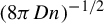 , where the ‘diffusion coefficient’
$D \approx 1/2$
 .
The weaker (but still open) claim that
$d_n \to 0$
 is equivalent to the condition that no kinks occur in the
$\mu $
 -limit set
$\Omega _\mu (f_{18})$
 . By [Reference Boyer, Delacourt, Sablik and Kari1, Proposition 2.10], the
$\mu $
 -limit set of every CA g is shift-recurrent, meaning that if w occurs in
$\Omega _\mu (g)$
 , then there exists a word u such that
$wuw$
 occurs in
$\Omega _\mu (g)$
 as well. Hence, for the weaker claim, it would be enough to prove that
 and that for some
$k \in \mathbb {N}$
 , no word with k kinks occurs in the generic limit set
 . We have shown that the latter claim is false for
$k \leq 2$
 .
Open problem 6.2. Characterize the language of the generic limit set  .
Open problem 6.3. Do we have  for the uniform Bernoulli measure
$\mu $
 ?
Acknowledgement
I.A.T. was supported by the Academy of Finland under grant 346566.

















 Open access

