1. Introduction
The complex Airy operator in  ${L^2}({\mathbb{R}})$
 \begin{equation}
A_0 = -\partial_x^2 + i x, \quad {\operatorname{Dom}}(A_0) = {W^{2,2}({\mathbb{R}})} \cap {\operatorname{Dom}}(x),
\end{equation}
and the corresponding realizations in  ${L^2}({\mathbb{R}}_+)$ and in
 ${L^2}(a, b)$ appear in various contexts, e.g. in the study of resonances [Reference Herbst30], superconductivity [Reference Almog1, Reference Almog, Helffer and Pan3, Reference Rubinstein, Sternberg and Zumbrun40], the Bloch–Torrey equation [Reference Grebenkov and Helffer24, Reference Grebenkov, Helffer and Henry25], MRI [Reference Grebenkov23], hydrodynamics [Reference Shkalikov45], control theory [Reference Beauchard, Helffer, Henry and Robbiano12], spectral instability [Reference Henry29], spectral approximation in domain truncations [Reference Semorádová and Siegl43], asymptotic description of pseudospectra of Schrödinger operators [Reference Arnal and Siegl7], completeness properties of the eigensystem and similarity to a normal operator [Reference Savchuk and Shkalikov42, Reference Tumanov and Shkalikov50], momenta with complex magnetic fields, quasi-self-adjoint Quantum Mechanics and Hardy-type inequalities in
 ${\mathbb{R}}^2$ [Reference Krejčiřík32] - see also [Reference Helffer28], [Reference Helffer27, Sec. 14.3, Sec. 14.5].
The crucial aspect of (1.1) is that it represents a tractable non-self-adjoint differential operator for which more explicit methods can be applied. In addition, more complicated operators in certain asymptotic regimes (e.g. the semi-classical one or those with large spectral parameter) can often be reduced to the analysis of the Airy operator. At the same time, the properties of A 0 already exhibit many striking and “highly non-self-adjoint” features. In particular:
(i) A 0 is m-accretive, has compact resolvent and
 $\sigma(A_0) = \emptyset$;
(ii) the resolvent norm only depends on
$\operatorname{Re} z$ and grows super-exponentially at
$+\infty$
(1.2)\begin{equation}
\| (A_0 - \operatorname{Re} z)^{-1} \| = \sqrt{\tfrac{\pi}{2}} (\operatorname{Re} z)^{-\frac14} \exp\left(\tfrac43 (\operatorname{Re} z)^{\frac32} \right) (1 + o(1)), \quad \operatorname{Re} z \to +\infty;
\end{equation}(iii) the semigroup St generated by
$-A_0$ is explicit and decays super-exponentially
\begin{equation*}
\|S_t\| = \exp( - \tfrac{t^3}{12}), \quad t \gt 0.
\end{equation*}


For details, see e.g. [Reference Helffer27, Sec. 14.3, Sec. 14.5]. The asymptotic equality (1.2) was proved in [Reference Bordeaux Montrieux13, Cor. 1.4] using pseudo-differential operator techniques within a semi-classical framework pioneered in [Reference Dencker, Sjöstrand and Zworski16]. It improved an earlier estimate, presented in [Reference Martinet35] (see also [Reference Bordeaux Montrieux13, Prop. 2.10] or [Reference Helffer27, Prop. 14.11]), which was derived via an analysis of the corresponding semigroup (see [Reference Bordeaux Montrieux13, Sec. 1]).
One of the reasons why the precise results summarized above are available is that, by transporting A 0 to the Fourier side (via  $\mathscr F A_0 \mathscr F^{-1}$, where
 $\mathscr F$ denotes the Fourier transform), one obtains the first-order operator
 \begin{equation*}
A_2 = -\partial_x + x^2, \quad {\operatorname{Dom}}(A_2) = {W^{1,2}({\mathbb{R}})} \cap {\operatorname{Dom}}(x^2)
\end{equation*}
(where we have retained x to denote the independent variable). In this paper, our main objective is to study generalized Airy operators in  ${L^2}({\mathbb{R}})$
 \begin{equation}
A = -\partial_x + W(x),
\end{equation}
where W is a non-negative, even, eventually increasing function which is unbounded at infinity, see Assumption 3.1 for details. Operators (1.3) share many properties of the complex Airy operator (1.1). In particular, they are m-accretive, have compact resolvent and empty spectrum, see Proposition 2.1 proved in [Reference Arnal and Siegl7, App. A]. Our goal here is to analyze precisely the resolvent and semigroup norms.
Our motivation originates in the analysis of pseudospectra of Schrödinger operators with complex potentials in [Reference Arnal and Siegl7] and of wave operators with unbounded damping in [Reference Arnal4], where the resolvent norm of A enters the asymptotic formulas for the level curves of the pseudospectra, see more details below and in Sub-section 6.1. Nonetheless, operators (1.3) furnish particularly simple instances, tractable by relatively elementary methods, that already exhibit the sort of pathologies found in more complex non-self-adjoint operators. Moreover, the flexibility in the rate of growth of W at infinity permits a wide range of resolvent and semigroup norm behaviours (see examples below and Examples 4.3, 5.3). These can in turn be used to address the optimality of abstract resolvent upper bounds based on Carleman-type estimates (see details below and in Sub-section 6.2).
Our main finding, Theorem 4.2, states that, if W satisfies Assumption 3.1, then
 \begin{equation}
\| (A - \lambda)^{-1} \| = \sqrt{\pi} (W'(x_{\lambda}))^{-\frac12} \exp \left(2 f_{\lambda}(x_{\lambda})\right) (1 + o(1)), \quad \lambda \to +\infty,
\end{equation}
with  $x_{\lambda} \gt 0$ the (positive) turning point of W defined by
 $W(x_{\lambda}) = \lambda$ and fλ the primitive of W defined by
 \begin{equation*}
f_{\lambda}(x) := \int_{0}^{x} (\lambda - W(t)) {{\rm d}} t, \quad x \in {\mathbb{R}};
\end{equation*}
note that, as for A 0, the resolvent norm is independent of  $\operatorname{Im} \lambda$.
This result is in agreement with (1.2), where  $W(x) = x^2$, and it yields a variety of rates for other examples of W, namely as
 $\lambda \to +\infty$,
 \begin{align*}
W(x) &= \log \langle x \rangle, & \| (A - \lambda)^{-1} \| &= \sqrt{\pi} \exp\left(2 \sqrt{e^{2 \lambda} - 1} + \lambda/2 - \pi\right) (1 + o(1)),\\
W(x) &= |x|^p, & \| (A - \lambda)^{-1} \| &= \sqrt{\tfrac{\pi}{p}} \lambda^{\frac{1 - p}{2 p}} \exp\left(\tfrac{2 p}{p + 1} \lambda^{\frac{1 + p}{p}}\right) (1 + o(1)), \ p \gt 0, \\
W(x) &= e^{|x|}, & \| (A - \lambda)^{-1} \| &= \sqrt{\pi} \lambda^{-\frac12} \exp\left(2 \lambda \log(\lambda) (1 + o(1))\right) (1 + o(1));
\end{align*}
see Example 4.3. It is apparent that the more slowly W grows the larger the resolvent will be: in the above examples, the largest resolvent corresponds to  $W(x) = \log \langle x \rangle$. A similar behaviour can be observed for one-dimensional Schrödinger operators with complex potentials (see [Reference Arnal and Siegl7, Sec. 7]).
In addition, in Theorem 5.1, we find the C 0-semigroup St generated by −A and calculate its norm. The latter decays in direct proportion to the growth of W, e.g.
 \begin{align*}
W(x) &= \log \langle x \rangle, & \| S_t \| &= \langle \tfrac t2 \rangle^{-t} \exp\left(t - \pi\right) (1 + o(1)), & &t \to +\infty,\\
W(x) &= |x|^p, & \| S_t \| &= \exp \left(-\tfrac{2^{-p}}{p + 1} t^{p + 1}\right), & &t \ge 0, \ p \gt 0,\\
W(x) &= e^{|x|}, & \| S_t \| &= \exp\left(-2 e^{\frac{t}{2}} (1 + o(1))\right), & &t \to +\infty,
\end{align*}
i.e. rapidly growing functions such as  $W(x) = e^{|x|}$ show faster semigroup decay; see Example 5.3 for more details.
As indicated above, the resolvent norm of A 0 and that of A appear in the asymptotic formulas for the shape of the pseudospectra of second-order differential operators. In [Reference Arnal and Siegl7, Prop. 5.1], it was shown that, for a wide class of Schrödinger operators with complex potential unbounded at infinity,  $H = -\partial_x^2 + i V$, in
 ${L^2}({\mathbb{R}}_+)$ (see [Reference Arnal and Siegl7, Asm. 3.1]), the norm of the resolvent of H along curves
 $\lambda_b = a(b) + i b$ inside the numerical range and adjacent to the imaginary axis can be estimated precisely as a function of the norm of the resolvent of A 0
 \begin{equation*}
\|(H - \lambda_b)^{-1} \| = \| (A_0 - \mu_b)^{-1} \| \left( V'(x_b) \right)^{-\frac{2}{3}} (1 + o(1)), \quad b \to +\infty,
\end{equation*}
where  $x_b \gt 0$ is the turning point of V determined by
 $V(x_b) = b$ and
 $\mu_b = a(b) ( V'(x_b))^{-\frac{2}{3}}$. Employing (1.2), this in turn yields the asymptotic shape of the ɛ-pseudospectra (with ɛ > 0)
 \begin{equation*}
a(b) = \left(\tfrac34\right)^{\frac23} V'(x_b)^\frac23 (\log(V'(x_b)^\frac23 \varepsilon^{-1}))^{\frac23} (1 + o(1)), \quad b \to +\infty;
\end{equation*}
see [Reference Arnal and Siegl7, Sub-sec. 5.1] for details and also [Reference Bordeaux Montrieux13] for results on semi-classical operators.
Operators A with  $W(x) = |x|^p$, p > 0, which we denote by
 $A_p := -\partial_x + |x|^p$, play a similar role to that outlined above for A 0 when estimating the norm of the resolvent for Schrödinger operators
 $H = -\partial_x^2 + i V$ in
 ${L^2}({\mathbb{R}})$ where V is even, unbounded at infinity and regularly varying with index of variation equal to p (see [Reference Arnal and Siegl7, Asm. 4.1]). Along curves
 $\lambda_a = a + i b(a)$ inside the numerical range and adjacent to the real axis (see [Reference Arnal and Siegl7, Thm. 4.2]), we have
 \begin{equation}
\| (H - \lambda_a)^{-1} \| = \| (A_p - \mu_a)^{-1} \| (V(t_a))^{-1} ( 1 + o(1)), \quad a \to +\infty,
\end{equation}
where  $t_a \gt 0$ is the solution of
 $t_a V(t_a) = 2 \sqrt{a}$ and
 $\mu_a = b(a) (V(t_a))^{-1}$. Combining (1.5) and (1.4) in the particular case
 $V(x) = x^{2m}$, one finds the asymptotic shape of the ɛ-pseudospectra
 \begin{equation*}
b(a) = \left(\tfrac{2m + 1}{2m}\right)^{\frac{2m}{2m + 1}} a^{\frac{m}{2m + 1}} \left(\log(a^{\frac{m}{2m + 1}} \varepsilon^{-1}) \right)^{\frac{2m}{2m + 1}} (1 + o(1)), \quad a \to +\infty,
\end{equation*}
see Sub-section 6.1.1 for details.
Operators of the general form  $A := -\partial_x + a(x)$ emerge in the study of the quadratic operator family
 $T(\lambda) = -\partial_x^2 + 2 \lambda a(x) + \lambda^2$,
 $\lambda \in {\mathbb{C}}$, associated with the one-dimensional wave equation with unbounded damping
 $a(x) \ge 0$. Similarly to the Schrödinger operators above, we discuss the asymptotic shape of level curves of
 $\|T(\lambda)^{-1}\|$ in Sub-section 6.1.2.
The operators (1.3) with W satisfying Assumption 3.1 have compact resolvent (see Proposition 2.1). Moreover, depending on the rate of growth of W, they belong to certain ideals of compact operators, e.g. Schatten classes, see Sub-section 6.2. Estimates of the norm of the resolvent for elements in trace ideals of compact operators go back to the early 20th century with the work of T. Carleman on integral operators. More recently, upper bounds have been found for (abstract) non-normal compact operators in the context of the analysis of their spectral behaviour under perturbation (see [Reference Bandtlow9–Reference Bandtlow and Güven11, Reference Sarıhan and Bandtlow41]). We shall review these bounds in Sub-section 6.2 in the light of our own findings. It is remarkable that the simple differential operators (1.3) (and also one-dimensional Schrödinger operators with imaginary monomial potentials) are close to exhausting the abstract bounds which do not take into account any particular structure of the operator besides the singular values of the resolvent.
Unlike some of the research mentioned earlier, our methods are relatively elementary. The two main tools used in the proof of Theorem 4.2 are Schur’s test with weights (see Sub-section 2.2) and an extension of Laplace’s method for integrals depending on a large parameter (see Lemma 4.5). The proof of (1.4) is structured in three steps:
(1) in Proposition 4.6, we use Schur’s test to prove that a certain integral operator,
$T_{k_{\lambda}}$ (see (2.3) and (4.8)), is bounded in
${L^2}$ and we find an upper bound;(2) in Proposition 4.7, we show that the upper bound found in the previous step is optimal;
(3) in the last step, the theorem’s proof, it is shown that
$T_{k_{\lambda}}$ is in fact the resolvent operator
$(A - \lambda)^{-1}$.


The remainder of the paper is structured as follows. Section 2 introduces our notation and recalls some fundamental tools applied later on. Section 3 states our assumptions. Section 4 is devoted to formulating and proving our estimate for the norm of the resolvent. Section 5 describes the C 0-semigroup generated by −A and calculates its norm. In Section 6, we apply our findings in two different contexts. Firstly (Sub-section 6.1), we derive the level curves for the norm of the resolvent in the particular cases outlined earlier (Schrödinger operators with complex potentials and the quadratic operator family associated with the damped wave equation). Secondly (Sub-section 6.2), we show that upper bounds for the resolvent of elements in certain classes of compact operators derived in [Reference Bandtlow9, Reference Sarıhan and Bandtlow41] using abstract methods are in fact optimal.
2. Notation and preliminaries
We write  ${\mathbb{R}}_+ := (0, +\infty)$ and the characteristic function of a set E is denoted by χE. We use
 ${C_c^{\infty}({\mathbb{R}})}$ to represent the space of smooth functions with compact support. Unless otherwise stated, our underlying Hilbert space shall be
 ${L^2}({\mathbb{R}})$. The L 2 inner product shall be denoted by
 $\langle \cdot, \cdot \rangle$ and the L 2 norm by
 $\| \cdot \|$. In the one-dimensional setting, we will denote the first and second-order differential operators by
 $\partial_x$ and
 $\partial_x^2$, respectively. We will also appeal to the Sobolev spaces
 ${W^{1,2}({\mathbb{R}})}$ and
 ${W^{2,2}({\mathbb{R}})}$ (see e.g. [Reference Edmunds and Evans19, Sub-sec. V.3] for definitions).
If  $\mathcal H$ is a Hilbert space,
 $\mathscr L(\mathcal H)$ shall denote the (Banach) space of bounded linear operators on
 $\mathcal H$. For a closed, densely defined linear operator T on a Hilbert space
 $\mathcal H$, we will write as usual
 $\rho(T)$,
 $\sigma(T)$ and
 $\sigma_{p}(T)$ to denote its resolvent set, its spectrum and the set of its eigenvalues, respectively.
If  $\mathcal H$ is a Hilbert space, we will represent by
 $\mathscr K(\mathcal H)$ the set of compact operators on
 $\mathcal H$, which is a closed two-sided ideal in
 $\mathscr L(\mathcal H)$. For
 $0 \lt p \lt \infty$, we shall denote by
 $\mathcal S_{p,\infty}$ the Schatten-Lorentz class
 \begin{equation*}
\mathcal S_{p, \infty} := \left\{T \in \mathscr K(\mathcal H) : \| T \|_{p, \infty} := \underset{k \in \mathbb{N}}{\sup} \: k^\frac1{p} s_k(T) \lt \infty\right\},
\end{equation*}
where  $s_k(T)$ represents the kth singular value of T (such values are assumed to be listed in decreasing order and repeated according to their multiplicity). We refer the interested reader to e.g. [Reference Sarıhan and Bandtlow41, Sec. 3] and the references therein or to [Reference Peller38, App. 1.1] for details on the theory of these and similar classes.
To avoid introducing multiple constants whose exact value is inessential for our purposes, we write  $a \lesssim b$ to indicate that, given
 $a,b \ge 0$, there exists a constant C > 0, independent of any relevant variable or parameter, such that
 $a \le Cb$. The relation
 $a \gt rsim b$ is defined analogously whereas a ≈ b means that
 $a \lesssim b$ and
 $a \gt rsim b$.
2.1. Basic properties of generalized Airy operators
It has been shown (see [Reference Arnal and Siegl7, App. A]) that the following result holds, i.e. A shares the basic properties with the complex Airy operator A 0.
Proposition 2.1. Let  $W \in {L^{\infty}_{\rm loc}({\mathbb{R}}}) \cap C^1({\mathbb{R}}\setminus [-x_0,x_0])$, for some
 $x_0 \gt 0$, and
 \begin{equation*}
A := -\partial_x + W, \quad
{\operatorname{Dom}}(A) := \{u \in {L^2}({\mathbb{R}}) \, : \, -u' + W u \in {L^2}({\mathbb{R}}) \}.
\end{equation*}
Assuming  $W \ge 0$ a.e. and
 $\lim_{|x| \to +\infty} W(x) = +\infty$, then
(i) A is densely defined and m-accretive;
(ii) A has compact resolvent and
$\sigma(A) = \emptyset$;(iii) the adjoint operator reads
\begin{equation*}
A^* = \partial_x + W, \quad
{\operatorname{Dom}}(A^*) = \{u \in {L^2}({\mathbb{R}}) \, : \, u' + W u \in {L^2}({\mathbb{R}}) \}.
\end{equation*}


If, in addition, there exist  $\varepsilon \in (0,1)$ and M > 0 such that
 \begin{equation}
|W'(x)| \le \varepsilon |W(x)|^2 + M, \quad |x| \gt x_0,
\end{equation}
then
 \begin{equation*}
{\operatorname{Dom}}(A) = {\operatorname{Dom}}(A^*) = W^{1,2}({\mathbb{R}}) \cap {\operatorname{Dom}}(W)
\end{equation*}
and we have
 \begin{equation}
\begin{aligned}
\| A u \|^2 + \| u \|^2 &\geq C_A \left(\| u' \|^2 + \| W u \|^2 + \| u \|^2 \right), \quad u \in {\operatorname{Dom}}(A),
\\
\| A^* u \|^2 + \| u \|^2 &\geq C_{A^*} \left(\| u' \|^2 + \| W u \|^2 + \| u \|^2 \right), \quad u \in {\operatorname{Dom}}(A^*);
\end{aligned}
\end{equation}
the constants  $C_{A}, C_{A^*} \gt 0$ depend only on ɛ, M and
 $\|W \chi_{[-x_0,x_0]}\|_\infty$.
2.2. Schur’s test
Let Tk be the integral operator determined by the non-negative kernel  $k: {\mathbb{R}} \times {\mathbb{R}} \to [0, +\infty)$ i.e. formally
 \begin{equation}
T_k u(x) = \int_{{\mathbb{R}}} k(x,y) u(y) {{\rm d}} y, \quad x \in {\mathbb{R}}.
\end{equation}
Schur’s test states that, if there exist strictly positive measurable functions  $p, q$ on
 ${\mathbb{R}}$ and constants
 $\alpha, \beta \gt 0$ such that
 $k(x,y)$ satisfies
 \begin{equation}
\begin{aligned}
&\int_{\mathbb{R}} k(x,y) q(y){{\rm d}} y \le \alpha p(x) \quad \text{for almost every } x \in {\mathbb{R}},\\
&\int_{\mathbb{R}} k(x,y) p(x) {{\rm d}} x \le \beta q(y) \quad \text{for almost every } y \in {\mathbb{R}},
\end{aligned}
\end{equation}
then the operator Tk in (2.3) is well-defined for every  $u \in {L^2}({\mathbb{R}})$ and
 \begin{equation}
\| T_k \| \le \sqrt{\alpha \beta}
\end{equation}
(see e.g. [Reference Halmos and Sunder26, Thm. 5.2]).
3. Assumptions
We begin by listing the assumptions that W will obey throughout the rest of the paper.
Theorem 3.1. Suppose that  $W \in {L^{\infty}_{\rm loc}({\mathbb{R}}}) \cap C^2({\mathbb{R}} \setminus [-x_0, x_0])$, for some
 $x_0 \in {\mathbb{R}}_+$, with
 $W \ge 0$ a.e. and assume further that the following conditions are satisfied:
(i) W is even:
\begin{equation*}
W(-x) = W(x), \quad x \in {\mathbb{R}};
\end{equation*}(ii) W is unbounded and eventually increasing in
${\mathbb{R}}_+$:
\begin{equation*}
\lim_{x \to +\infty} W(x) = +\infty, \quad W'(x) \gt 0, \quad x \gt x_0;
\end{equation*}(iii) W has controlled derivatives: there exist
$\nu \in [-1, +\infty)$ such that
\begin{equation*}
W'(x) \lesssim W(x) x^{\nu}, \quad
|W''(x)| \lesssim W'(x) x^{\nu}, \quad x \gt x_0;
\end{equation*}(iv) W grows sufficiently fast: we have
\begin{equation*}
\Upsilon_1(x) = o(1), \quad |x| \to +\infty,
\end{equation*}where
\begin{equation*}
\Upsilon_1(x) := |x|^{\nu} |W'(x)|^{-\frac12},\quad |x| \gt x_0.
\end{equation*}


Remark 3.2. We make the following observations based on the above conditions.
(i) From Assumptions 3.1 (iii), (iv), we have
\begin{equation*}
\frac{|W'(x)|}{(W(x))^2} \lesssim \frac{|W'(x)|}{|W'(x)|^2 |x|^{-2 \nu}} = (\Upsilon_1(x))^2 = o(1), \quad |x| \to +\infty.
\end{equation*}It follows that (2.1) holds and therefore the domain of the corresponding generalized Airy operator separates
(3.1)\begin{equation}
A = -\partial_x + W(x), \quad {\operatorname{Dom}}(A) = {W^{1,2}({\mathbb{R}})} \cap {\operatorname{Dom}}(W).
\end{equation}(ii) Assumption 3.1 (iii) implies that, for any
$0 \lt \varepsilon \lt 1$, all sufficiently large
$|x|$ and
$|\delta| \le \varepsilon |x|^{-\nu}$, we can control the variation of W and that of W′ on intervals whose length is of order
$|x|^{-\nu}$
(3.2)(see [Reference Mityagin, Siegl and Viola36, Lem. 4.1]).\begin{equation}
\frac{W^{(j)}(x + \delta)}{W^{(j)}(x)} \approx 1, \quad j \in \{0, 1\},
\end{equation}(iii) The quantity
$\Upsilon_1(x)$ in Assumption 3.1 (iv) is the equivalent, for a first order differential operator such as A, of
$\Upsilon(x)$ for a Schrödinger operator in [Reference Arnal and Siegl7, Asm. 3.1 (iii)].


Example 3.3. Assumption 3.1 (iii) encompasses a wide range of unbounded W growing at very different rates, for example:
(i) logarithmic functions such as
$W(x) = \log \langle x \rangle^p$, p > 0;(ii) polynomial functions such as
$W(x) = |x|^p$, p > 0 - note that, when p = 2, we recover, via the Fourier transform, the complex Airy operator A 0 (see the comments to this effect in Section 1);(iii) exponential functions such as
$W(x) = e^{|x|^p}$, p > 0.


4. The norm of the resolvent operator
In this section, our aim is to provide an estimate of  $\| (A - \lambda)^{-1} \|$ as
 $\lambda \to +\infty$. Note that, since A is m-accretive, it is immediate that
 $\| (A - \lambda)^{-1} \| \le 1/|\lambda|$ for every λ < 0. Furthermore, it is sufficient to consider
 $\lambda \in {\mathbb{R}}$ since, for general
 $\lambda \in {\mathbb{C}}$, we have
 $(A - \lambda)^{-1} = U_{\operatorname{Im} \lambda}^{-1} (A - \operatorname{Re}\lambda)^{-1} U_{\operatorname{Im} \lambda}$, with the isometry
 $U_{a} u(x) = e^{i a x} u(x)$ for any
 $u \in {L^2}({\mathbb{R}})$ and
 $a \in {\mathbb{R}}$, and hence
 $\| (A - \lambda)^{-1} \| = \| (A - \operatorname{Re}\lambda)^{-1} \|$.
4.1. Statement of the result
By Assumption 3.1 (ii), there exists  $\lambda_0 \gt 0$ (e.g. take any
 $\lambda_0 \gt \| W \chi_{[0, x_0]} \|_{\infty}$) such that, for every
 $\lambda \ge \lambda_0$, the equation
 $W(x) = \lambda$ has a unique solution in
 ${\mathbb{R}}_+$ which we shall denote by xλ (the turning point of W), i.e.
 \begin{equation}
W(x_{\lambda}) = \lambda, \qquad x_\lambda \gt 0.
\end{equation}
Note that
 \begin{equation}
\lim_{\lambda \to +\infty} x_{\lambda} = +\infty.
\end{equation}
Furthermore, for every λ > 0 we define the real function
 \begin{equation}
f_{\lambda}(x) := \int_{0}^{x} (\lambda - W(t)) {{\rm d}} t, \quad x \in {\mathbb{R}}.
\end{equation}
Clearly  $f_{\lambda} \in W^{1,\infty}_{\mathrm{loc}}({\mathbb{R}}) \cap C^3({\mathbb{R}} \setminus [-x_0,x_0])$,
 $f_{\lambda}(0) = 0$ and
 \begin{equation}
f'_{\lambda}(x) = \lambda - W(x), \quad \text{a.e. in } {\mathbb{R}}, \quad f''_{\lambda}(x) = -W'(x), \quad x \in {\mathbb{R}} \setminus [-x_0, x_0].
\end{equation}
An elementary analysis provides the following properties for fλ.
Lemma 4.1. For λ > 0 and fλ as defined by (4.3), we have that fλ is an odd function and in addition
(i) fλ is unbounded
(4.5)\begin{equation}
\lim_{x \to +\infty} f_{\lambda}(x) = -\infty.
\end{equation}

Furthermore there exists  $\lambda_0 \gt 0$ such that for all
 $\lambda \ge \lambda_0$
(ii) The value xλ defined by (4.1) is a critical point
\begin{equation*}
f'_{\lambda}(x_{\lambda}) = 0, \quad f''_{\lambda}(x_{\lambda}) \lt 0.
\end{equation*}(iii) There exists
$x_{\lambda,0} \gt x_{\lambda}$ (which is unique in
${\mathbb{R}}_+$) such that
(4.6)\begin{gather}
f_{\lambda}(x_{\lambda,0}) = 0,
\end{gather}
\begin{gather*}
f_{\lambda}(x) \gt 0, \quad x \in (0, x_{\lambda,0}).
\end{gather*}


Proof. It is clear that, by (4.3) and Assumption 3.1 (i), fλ is odd.
(i) Let λ > 0 be arbitrary but fixed. Since, by Assumption 3.1 (ii), we have  $W(x) \to +\infty$ for
 $x \to +\infty$, it follows that there exists
 $x_1(\lambda) \gt 0$ such that
 \begin{equation*}
\lambda - W(x) \le -1, \quad x \ge x_1(\lambda).
\end{equation*}
Hence, for some  $C_{\lambda} \in {\mathbb{R}}$ and any
 $x \ge x_1(\lambda)$, we have
 \begin{equation*}
\begin{aligned}
f_{\lambda}(x) = \int_{0}^{x_1(\lambda)} (\lambda - W(t)) {{\rm d}} t + \int_{x_1(\lambda)}^{x} (\lambda - W(t)) {{\rm d}} t \le C_{\lambda} + x_1(\lambda) - x.
\end{aligned}
\end{equation*}
We therefore conclude that (4.5) holds.
(ii) Setting λ 0 as per definition (4.1) or larger, the statement is a direct consequence of (4.4), (4.1) and Assumption 3.1 (ii).
(iii) Let λ 0 be as in (ii) and let  $\lambda \ge \lambda_0$ be arbitrary but fixed. Since
 $f_{\lambda}(0) = 0$,
 $f'_{\lambda}(x) \gt 0$ for
 $x \in (0, x_{\lambda})$,
 $f'_{\lambda}(x) \lt 0$ for
 $x \in (x_{\lambda}, +\infty)$ (recall that
 $f'_{\lambda}(x) = - W(x) + \lambda$) and moreover, by (4.5),
 $f_{\lambda}(x)$ is eventually negative, we deduce that there exists a unique
 $x_{\lambda,0} \gt x_{\lambda}$ such that
 $f_{\lambda}(x_{\lambda,0}) = 0$ and
 $f_{\lambda}(x)$ must be strictly positive in
 $(0, x_{\lambda,0})$, as claimed.
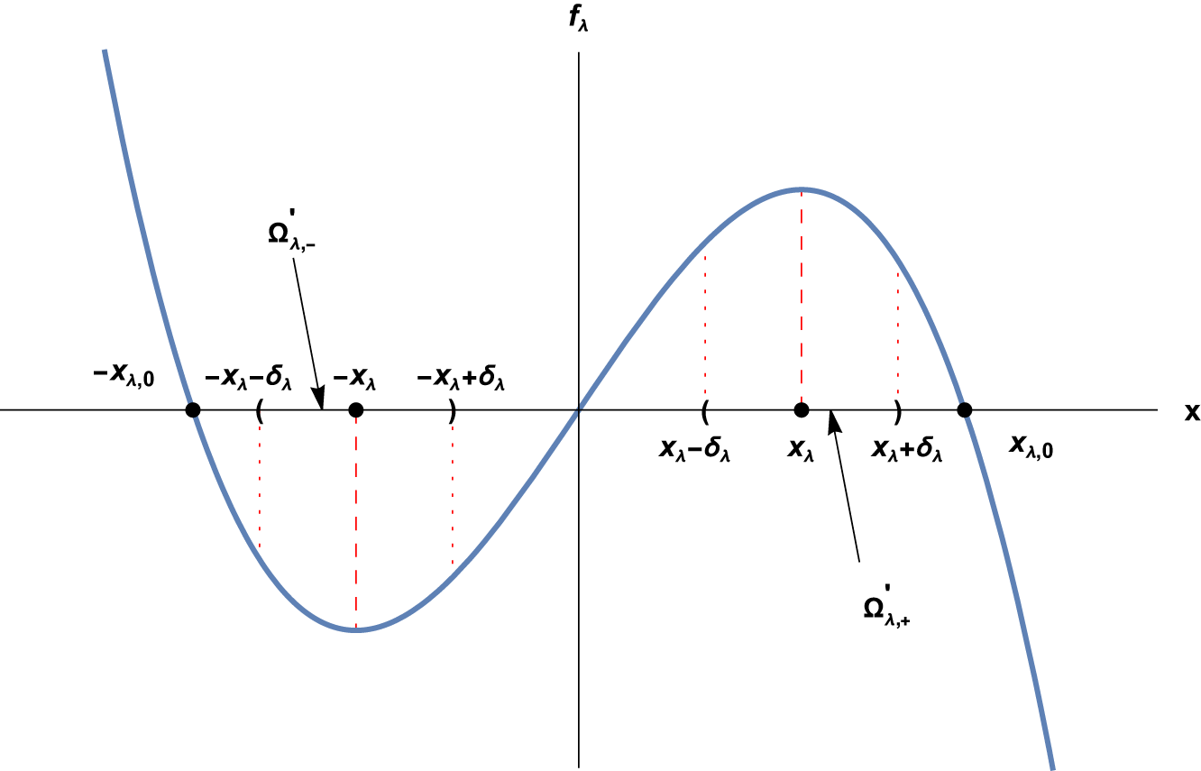
The behaviour of fλ is sketched in Fig. 4.1 (see also Definition (4.9) and Lemma 4.4).
Sketch of  $f_{\lambda}(x)$, defined by (4.3), for sufficiently large λ.

Our main result in this section is the following.
Theorem 4.2. Let W satisfy Assumption 3.1, let A be the generalized Airy operator (3.1) in  ${L^2}({\mathbb{R}})$ and let λ > 0. Then
 \begin{equation}
\| (A - \lambda)^{-1} \| = \sqrt{\pi} (W'(x_{\lambda}))^{-\frac12} \exp \left(2 f_{\lambda}(x_{\lambda})\right) (1 + o(1)), \quad \lambda \to +\infty,
\end{equation}
where xλ and fλ are defined by (4.1) and (4.3), respectively.
Example 4.3. In order to illustrate Theorem 4.2, we revisit the instances shown in Example 3.3.
(i) For the slowly-growing function
$W(x) = \log \langle x \rangle^{p}$, p > 0, it is straightforward to verify that
$W'(x) = p x \langle x \rangle^{-2}$,
$f_{\lambda}(x) = (\lambda + p) x - x W(x) - p \arctan(x)$ and
$x_{\lambda} = \sqrt{\exp(2 \lambda / p) - 1}$. This yields the estimate
\begin{align*}
\| (A - \lambda)^{-1} \| &= \sqrt{\frac{\pi}{p}} \exp\left(2 p \sqrt{\exp \left(\frac{2\lambda}{p} \right) - 1} + \frac{\lambda}{2 p} - p \pi\right)\nonumber \\ & \qquad (1 + o(1)), \quad \lambda \to +\infty.
\end{align*}(ii) For
$W(x) = |x|^{p}$, p > 0, we have
$W'(x) = p \operatorname{sgn}(x) |x|^{p - 1}$,
$f_{\lambda}(x) = x (\lambda - W(x) / (p + 1))$,
$x_{\lambda} = \lambda^{1/p}$ and the estimate
\begin{equation*}
\| (A - \lambda)^{-1} \| = \sqrt{\frac{\pi}{p}} \lambda^{\frac{1 - p}{2 p}} \exp\left(\frac{2 p}{p + 1} \lambda^{\frac{1 + p}{p}}\right) (1 + o(1)), \quad \lambda \to +\infty.
\end{equation*}We note that, in the particular case p = 2 (the complex Airy operator on the Fourier side), we recover the estimate found elsewhere (see e.g. [Reference Bordeaux Montrieux13, Cor. 1.4])
\begin{equation*}
\| (A - \lambda)^{-1} \| = \sqrt{\frac{\pi}{2}} \lambda^{-\frac14} \exp\left(\frac43 \lambda^{\frac32}\right) (1 + o(1)), \quad \lambda \to +\infty.
\end{equation*}(iii) For the fast-growing function
$W(x) = e^{|x|^{p}}$, p > 0, one can similarly check that
$W'(x) = p \operatorname{sgn}(x) |x|^{p-1} W(x)$,
$f_{\lambda}(x) = \lambda x - W(x) F_p(x)$, where
$F_p(x)$ denotes the generalized Dawson’s integral (see [Reference Olver, Olde Daalhuis, Lozier, Schneider, Boisvert, Clark, Miller and Saunders37, Sec. 7.16] or [Reference Dijkstra17, Eq. 1.1]), and
$x_{\lambda} = (\log(\lambda))^{\frac1{p}}$. The estimate of the resolvent norm as
$\lambda \to +\infty$ is
(note that
\begin{equation*}
\begin{aligned}
\| (A - \lambda)^{-1} \| &= \sqrt{\frac{\pi}{p}} \lambda^{-\frac12} (\log(\lambda))^{\frac{1-p}{p}} \exp\left(2 \lambda \left((\log(\lambda))^{\frac1{p}} - F_p\left((\log(\lambda))^{\frac1{p}}\right)\right)\right)\\
& \qquad\!\! (1 + o(1))
\end{aligned}
\end{equation*}
$F_p(x) = (1 / p) x^{1-p} (1 + \mathcal{O}(x^{-p}))$ for
$x \to +\infty$, see e.g. [Reference Olver, Olde Daalhuis, Lozier, Schneider, Boisvert, Clark, Miller and Saunders37, Secs. 7.16, 8.11] or [Reference Dijkstra17, Eq. 2.5]).


4.2. Proof of Theorem 4.2
To prove the theorem, we shall show that the integral operator  $T_{k_{\lambda}}$ with the kernel (for λ > 0 and fλ as in (4.3))
 \begin{equation}
k_{\lambda}(x,y) :=
\begin{cases}
e^{f_{\lambda}(y) - f_{\lambda}(x)}, & x \lt y,\\[1mm]
0, & x \ge y,
\end{cases}
\quad x, y \in {\mathbb{R}},
\end{equation}
is the resolvent  $(A - \lambda)^{-1}$. To this effect, we prove that
 $T_{k_{\lambda}}$ is bounded, establishing in the process that the right-hand side of (4.7) is an (asymptotic) upper bound for its norm (Proposition 4.6). We will then proceed to prove that the upper bound is in fact optimal (Proposition 4.7).
We begin by proving two lemmas that describe some further important properties of fλ. Let
 \begin{equation}
\Omega'_{\lambda,\pm} := \left( \pm x_{\lambda} - \delta_{\lambda}, \pm x_{\lambda} + \delta_{\lambda} \right), \quad \delta_{\lambda} := \delta x_{\lambda}^{-\nu}, \quad 0 \lt \delta \lt \frac 14,
\end{equation}
where δ will be determined in Lemmas 4.4 and 4.5 and  $\nu \ge -1$ (see Assumption 3.1 (iii)). The above choice for the width of
 $\Omega'_{\lambda,\pm}$ implies that W(x) is approximately equal to
 $W(x_{\lambda})$ inside those intervals (see Remark 3.2 (ii)), a fact which we shall repeatedly rely upon in the proofs below.
Lemma 4.4. Let W satisfy Assumption 3.1 and let xλ,  $x_{\lambda,0}$ and
 $\Omega'_{\lambda,+}$ be as defined in (4.1), (4.6) and (4.9), respectively. Then as
 $\lambda \to +\infty$, we have:
(i)
(4.10)\begin{equation}
x_{\lambda} \pm \delta_{\lambda} \approx x_{\lambda}.
\end{equation}(ii)
\begin{equation*}
\Omega'_{\lambda,+} \subset (0, x_{\lambda,0}).
\end{equation*}


Proof. (i) By (4.2) and  $\nu \ge -1$, we find as
 $\lambda \to +\infty$
 \begin{equation*}
x_{\lambda} \pm \delta_{\lambda} = x_{\lambda} (1 \pm \delta x_{\lambda}^{-1 - \nu}) \approx x_{\lambda}.
\end{equation*}
(ii) Since  $x_\lambda - \delta_{\lambda} \gt 0$ as
 $\lambda \to +\infty$ by (i), it is enough to prove
 $f_{\lambda}(x_{\lambda}+\delta_{\lambda}) \gt 0$ (see Lemma 4.1) for
 $\lambda \to +\infty$. For λ 0 as in the statement of Lemma 4.1 and any
 $\lambda \ge \lambda_0$, we have (with x 0 as in Assumption 3.1 and applying (4.4) and integration by parts)
 \begin{equation*}
\begin{aligned}
f_{\lambda}(x_{\lambda}) &= \int_{0}^{x_{\lambda}} (\lambda - W(t)) {{\rm d}} t = \int_{0}^{x_0} (\lambda - W(t)) {{\rm d}} t + \int_{x_0}^{x_{\lambda}} (\lambda - W(t)) {{\rm d}} t\\
&= \int_{0}^{x_0} (\lambda - W(t)) {{\rm d}} t - (\lambda - W(x_0)) x_0 + \int_{x_0}^{x_{\lambda}} t W'(t) {{\rm d}} t\\
&= \int_{0}^{x_0} (W(x_0) - W(t)) {{\rm d}} t + \int_{x_0}^{x_{\lambda}} t W'(t) {{\rm d}} t.
\end{aligned}
\end{equation*}
The first term in the preceding line is a constant, whereas the second one diverges as  $\lambda \to +\infty$ (we may assume
 $x_0 \ge 1$), hence
 \begin{equation*}
f_\lambda(x_{\lambda}) = \int_{x_0}^{x_{\lambda}} t W'(t) {{\rm d}} t \; (1 + o(1)) \gt rsim \int_{x_{\lambda} - \varepsilon x_{\lambda}^{-\nu}}^{x_{\lambda}} t W'(t) {{\rm d}} t,
\end{equation*}
for sufficiently small ɛ > 0 and  $\lambda \to +\infty$. By (3.2), we deduce that
 $\min \{W'(t) : t \in [x_{\lambda} - \varepsilon x_{\lambda}^{-\nu}, x_{\lambda}]\} \approx W'(x_{\lambda})$. Furthermore,
 $x_{\lambda} - \varepsilon x_{\lambda}^{-\nu} \approx x_{\lambda}$ for small enough ɛ > 0 by (4.10). It follows
 \begin{equation}
f_{\lambda}(x_{\lambda}) \gt rsim x_{\lambda} W'(x_{\lambda}) \varepsilon x_{\lambda}^{-\nu} \approx W'(x_{\lambda}) x_{\lambda}^{1 - \nu}, \quad \lambda \to +\infty.
\end{equation}
 \begin{equation}
\frac{(\Upsilon_1(x_{\lambda}))^{-2}}{f_{\lambda}(x_{\lambda})} = \frac{W'(x_{\lambda})}{f_{\lambda}(x_{\lambda}) x_{\lambda}^{2 \nu}} \lesssim \frac{W'(x_{\lambda})}{W'(x_{\lambda}) x_{\lambda}^{1 + \nu}} = \mathcal{O}(1), \quad \lambda \to +\infty,
\end{equation}
and hence (with  $\xi_{\lambda} \in (x_{\lambda}, x_{\lambda} + \delta_{\lambda})$ and applying (4.4))
 \begin{equation}
\begin{aligned}
f_{\lambda}(x_{\lambda} + \delta_{\lambda}) &= f_{\lambda}(x_{\lambda}) + f'_{\lambda}(x_{\lambda}) \delta_{\lambda} + \frac12 f''_{\lambda}(x_{\lambda}) \delta_{\lambda}^2 + \frac16 f'''_{\lambda}(\xi_{\lambda}) \delta_{\lambda}^3\\
&= f_{\lambda}(x_{\lambda}) \left(1 - \frac12 \frac{W'(x_{\lambda})}{f_{\lambda}(x_{\lambda})} \delta_{\lambda}^2 \left(1 + \frac13 \frac{W''(\xi_{\lambda})}{W'(x_{\lambda})} \delta_{\lambda}\right)\right)\\
&= f_{\lambda}(x_{\lambda}) \left(1 - \frac12 \delta^2 \frac{(\Upsilon_1(x_{\lambda}))^{-2}}{f_{\lambda}(x_{\lambda})} \left(1 + \frac13 \frac{W''(\xi_{\lambda})}{W'(x_{\lambda})} \delta_{\lambda}\right)\right).
\end{aligned}
\end{equation}
By (4.12), we obtain  $\delta^2 (\Upsilon_1(x_{\lambda}))^{-2} / f_{\lambda}(x_{\lambda}) = \mathcal{O}(\delta^2)$ and, by Assumption 3.1 (iii), (4.10) and (3.2), we deduce
 $\vert W''(\xi_\lambda)\vert\delta_\lambda/W'(x_\lambda)\lesssim\delta$. Hence, using (4.13) and choosing δ > 0 sufficiently small in (4.9), we have
 \begin{equation*}
f_{\lambda}(x_{\lambda} + \delta_{\lambda}) \gt f_{\lambda}(x_{\lambda}) \left(1 - \mathcal{O}(\delta^2)\right) \gt 0, \quad \lambda \to +\infty,
\end{equation*}
as claimed.
Our next result is the critical ingredient in the calculation of the estimate (4.7). It uses the idea of Laplace’s method and slightly extends it to provide suitable estimates for the proof of our claim.
Lemma 4.5. Let λ > 0 and let  $x_{\lambda}, \Omega'_{\lambda,\pm}, f_{\lambda}(x)$ be as defined by (4.1), (4.9) and (4.3), respectively. Then for any M > 0 and with
 $\lambda \to +\infty$
 \begin{align} I_{\lambda,+} := \int_{\Omega'_{\lambda,+}} e^{M f_{\lambda}(x)} {{\rm d}} x &= \sqrt{\frac{2 \pi}{M}} (W'(x_{\lambda}))^{-\frac12} e^{M f_{\lambda}(x_{\lambda})} (1 + o(1)), \quad
\end{align}
 \begin{align} I_{\lambda,-} := \int_{\Omega'_{\lambda,-}} e^{M f_{\lambda}(x)} {{\rm d}} x &= \sqrt{\frac{2 \pi}{M}} (W'(x_{\lambda}))^{-\frac12} e^{M f_{\lambda}(x_{\lambda})} o(1). \quad
\end{align}
Proof. For  $\lambda_0 \gt 0$ as in Lemma 4.1 and any
 $\lambda \ge \lambda_0$, let
 $\rho := |f''_{\lambda}(x_{\lambda})|^{-\frac12} \gt 0$ and
 $\Omega'_{\lambda,\rho} := (-\delta_{\lambda} \rho^{-1}, \delta_{\lambda} \rho^{-1})$. For every
 $y \in \Omega'_{\lambda,\rho}$, we define
 \begin{equation}
g_{\lambda}(y) := f_{\lambda}(\rho y + x_{\lambda}).
\end{equation}
Taylor-expanding gλ around 0 and using the facts that  $g'_{\lambda}(0) = \rho f'_{\lambda}(x_{\lambda}) = 0$ (refer to (4.1) and (4.4)) and
 $g''_{\lambda}(0) = \rho^2 f''_{\lambda}(x_{\lambda}) = -1$ (by Assumption 3.1 (ii), (4.4) and our choice of ρ) we obtain
 \begin{equation}
g_{\lambda}(y) = g_{\lambda}(0) - \frac12 y^2 + \frac16 g'''_{\lambda}(s y) y^3, \quad y \in \Omega'_{\lambda,\rho},
\end{equation}
where  $s = s(y, \lambda)$ and
 $0 \lt s \lt 1$. Furthermore, by (4.4) and Assumption 3.1 (iii)
 \begin{equation*}
\begin{aligned}
|g'''_{\lambda}(s y)| &= |f'''_{\lambda}(\rho s y + x_{\lambda})| \rho^3 = \frac{|W''(\rho s y + x_{\lambda})|}{(W'(x_{\lambda}))^{\frac32}}\\
&\lesssim \frac{W'(\rho s y + x_{\lambda})}{(W'(x_{\lambda}))^{\frac32}} (\rho s y + x_{\lambda})^{\nu}.
\end{aligned}
\end{equation*}
For any  $y \in \Omega'_{\lambda,\rho}$, we have
 $|\rho s y| \le \frac12 x_{\lambda}^{-\nu}$ by (4.9) and hence
 $(x_{\lambda}^{-1} \rho s y + 1)^{\nu} \approx 1$, i.e.
 $(\rho s y + x_{\lambda})^{\nu} \approx x_{\lambda}^{\nu}$. Combining this fact with (3.2), we deduce
 \begin{equation}
|g'''_{\lambda}(s y)| \lesssim (\rho s y + x_{\lambda})^{\nu} (W'(x_{\lambda}))^{-\frac12} \lesssim \Upsilon_1(x_{\lambda}), \quad y \in \Omega'_{\lambda,\rho}.
\end{equation}
Observing that  $\delta_{\lambda} \rho^{-1} = (\Upsilon_1(x_{\lambda}))^{-1} \delta$, we have
 $|g'''_{\lambda}(s y) y| \lesssim \delta$ for any
 $y \in \Omega'_{\lambda,\rho}$ and consequently, by choosing a sufficiently small δ in (4.9), we get
 \begin{equation}
1 - \frac13 g'''_{\lambda}(s y) y \approx 1.
\end{equation}
In order to estimate  $I_{\lambda,+}$, we change variable
 $x \to \rho y + x_{\lambda}$ and apply (4.16) and (4.17) to derive
 \begin{equation}
I_{\lambda,+} = e^{M g_{\lambda}(0)} \rho \int_{{\mathbb{R}}} e^{-\frac12 M y^2 (1 - \frac13 g'''_{\lambda}(s y) y)} \chi_{\Omega'_{\lambda,\rho}}(y) {{\rm d}} y.
\end{equation}
Note that, by (4.19), there exists some C > 0 such that
 \begin{equation*}
e^{-\frac12 M y^2 (1 - \frac13 g'''_{\lambda}(s y) y)} \chi_{\Omega'_{\lambda,\rho}}(y) \le e^{-\frac12 C M y^2}, \quad y \in {\mathbb{R}}, \quad \lambda \ge \lambda_0.
\end{equation*}
Furthermore,  $\Upsilon_1(x_{\lambda}) = o(1)$ as
 $\lambda \to +\infty$ by Assumption 3.1 (iv) and therefore
 $\delta_{\lambda} \rho^{-1} \to +\infty$ for
 $\lambda \to +\infty$. Noting also (4.18), we have for any fixed
 $y \in {\mathbb{R}}$
 \begin{equation*}
\lim_{\lambda \to +\infty} e^{-\frac12 M y^2 (1 - \frac13 g'''_{\lambda}(s y) y)} \chi_{\Omega'_{\lambda,\rho}}(y) = e^{-\frac12 M y^2}.
\end{equation*}
Finally, we apply the dominated convergence theorem to (4.20) to deduce
 \begin{equation*}
I_{\lambda,+} = e^{M g_{\lambda}(0)} \rho \sqrt{\frac{2 \pi}{M}} (1 + o(1)), \quad \lambda \to +\infty,
\end{equation*}
which yields (4.14).
To prove (4.15), we change variable in the integrand of  $I_{\lambda,-}$ (
 $x \to -\rho y - x_{\lambda}$) to obtain (using the fact that fλ is odd and arguing as above)
 \begin{equation*}
\begin{aligned}
I_{\lambda,-} &= e^{-M g_{\lambda}(0)} \rho \int_{{\mathbb{R}}} e^{\frac12 M y^2 (1 - \frac13 g'''_{\lambda}(s y) y)} \chi_{\Omega'_{\lambda,\rho}}(y) {{\rm d}} y\\
&\le e^{-M g_{\lambda}(0)} \rho \int_{{\mathbb{R}}} e^{\frac12 C' M y^2} \chi_{\Omega'_{\lambda,\rho}}(y) {{\rm d}} y = 2 e^{-M g_{\lambda}(0)} \rho \int_{0}^{\delta_{\lambda} \rho^{-1}} e^{\frac12 C' M y^2} {{\rm d}} y,
\end{aligned}
\end{equation*}
with some  $C' \gt 0$. It is straightforward to verify that
 $e^{-x^2} x \int_{0}^{x} e^{y^2} {{\rm d}} y = \mathcal{O}(1)$ as
 $x \to +\infty$ and hence
 \begin{equation*}
\begin{aligned}
I_{\lambda,-} &\lesssim e^{-M g_{\lambda}(0)} \rho \frac{e^{\frac12 C' M \delta_{\lambda}^2 \rho^{-2}}}{\delta_{\lambda} \rho^{-1}}\\
&= (W'(x_{\lambda}))^{-\frac12} e^{M f_{\lambda}(x_{\lambda})} \left(\delta^{-1} \Upsilon_1(x_{\lambda}) e^{-2 M f_{\lambda}(x_{\lambda}) \left(1 - \frac{C' \delta^2 (\Upsilon_1(x_{\lambda}))^{-2} }{4 f_{\lambda}(x_{\lambda})}\right)}\right),
\end{aligned}
\end{equation*}
for  $\lambda \to +\infty$. Recalling (4.12) and choosing an adequately small value for δ > 0 in (4.9), it follows that
 \begin{equation*}
1 - \delta^2 \frac{C' (\Upsilon_1(x_{\lambda}))^{-2}}{4 f_{\lambda}(x_{\lambda})} \gt 0,\quad \lambda \to +\infty.
\end{equation*}
We have M > 0 by assumption and it was shown in Lemma 4.1 (iii) that  $f_\lambda(x_{\lambda}) \gt 0$ for large enough λ; furthermore, by Assumption 3.1 (iv),
 $\Upsilon_1(x_{\lambda}) = o(1)$ as
 $\lambda \to +\infty$. Hence, we conclude that (4.15) holds.
4.2.1. The upper bound
With λ > 0 and kλ given by (4.8), we let  $T_{k_{\lambda}}$ be the associated integral operator as in (2.3). Furthermore, we introduce the weight functions in
 ${\mathbb{R}}$
 \begin{equation}
\begin{aligned}
p_{\lambda}(x) &=
\begin{cases}
e^{-f_{\lambda}(x)}, & x \in [-x_{\lambda} - \delta_{\lambda}, x_{\lambda} + \delta_{\lambda}],\\[1mm]
e^{-f_{\lambda}(x_{\lambda} + \delta_{\lambda})}, & x \gt x_{\lambda} + \delta_{\lambda},\\[1mm]
e^{-f_{\lambda}(-x_{\lambda} - \delta_{\lambda})}, & x \lt -x_{\lambda} - \delta_{\lambda},
\end{cases}
\\
q_{\lambda}(y) &=
\begin{cases}
e^{f_{\lambda}(y)}, & y \in [-x_{\lambda} - \delta_{\lambda}, x_{\lambda} + \delta_{\lambda}],\\[1mm]
e^{f_{\lambda}(x_{\lambda} + \delta_{\lambda})}, & y \gt x_{\lambda} + \delta_{\lambda},\\[1mm]
e^{f_{\lambda}(-x_{\lambda} - \delta_{\lambda})}, & y \lt -x_{\lambda} - \delta_{\lambda},
\end{cases}
\end{aligned}
\end{equation}
where xλ and δλ are defined in (4.1) and (4.9), respectively. Note that the choice of weights is motivated to ensure that the resulting constants  $\alpha, \beta$ in Schur’s test (see Sub-section 2.2) are optimal, which cannot be achieved with the trivial weights
 $p_{\lambda}(x) = q_{\lambda}(x) = 1$.
A heuristic argument behind selecting these particular weights is that Schur’s test for a compact integral operator T with a non-negative kernel becomes optimal if the weight is selected as the eigenfunction of  $T^*T$ corresponding to the largest eigenvalue, see e.g. [Reference Tao46, Rem. 5.10]. We do not have the eigenfunctions of
 $(A-\lambda)^*(A-\lambda)$ explicitly, nonetheless,
 $e^{-f_\lambda}$ solves
 $-u' + (W-\lambda) u =0$ (and
 $e^{f_\lambda}$ solves
 $u' + (W-\lambda) u =0$) and it turns out that the choice in (4.21) indeed provides the optimal upper bound for large λ in Proposition 4.6. A modification of
 $e^{\pm f_\lambda}$ is also used in the lower bound in Proposition 4.7 (see also the remark below its proof).
Proposition 4.6. Let W satisfy Assumption 3.1 and let λ > 0 and  $T_{k_{\lambda}}$ be the integral operator associated with the kernel (4.8). Then
 $T_{k_{\lambda}}$ is a bounded operator on
 ${L^2}({\mathbb{R}})$ and moreover
 \begin{equation}
\| T_{k_{\lambda}} \| \le \sqrt{\pi} (W'(x_{\lambda}))^{-\frac12}\exp \left(2 f_{\lambda}(x_{\lambda})\right) (1 + o(1)), \quad \lambda \to +\infty,
\end{equation}
where xλ and fλ are defined as in (4.1) and (4.3), respectively.
Proof. Our task is to estimate the integrals
 \begin{equation*}
\begin{aligned}
I_{\lambda}(x) &:= \int_{{\mathbb{R}}} k_{\lambda}(x,y) q_{\lambda}(y) {{\rm d}} y,\\
J_{\lambda}(y) &:= \int_{{\mathbb{R}}} k_{\lambda}(x,y) p_{\lambda}(x) {{\rm d}} x,
\end{aligned}
\quad x, y \in {\mathbb{R}}, \quad \lambda \to +\infty,
\end{equation*}
with  $k_{\lambda}(x,y)$ as in (4.8) and
 $p_{\lambda}(x), q_{\lambda}(y)$ as in (4.21). In what follows, we shall assume
 $\lambda \ge \lambda_0$ with λ 0 as in Lemma 4.1.
We split  ${\mathbb{R}}$ into subintervals and evaluate
 $I_{\lambda}(x)$ in each one in turn.
(i)
$ \underline{x \in [x_{\lambda} + \delta_{\lambda}, +\infty)} $
\begin{equation*}
\begin{aligned}
I_{\lambda}(x) &= e^{-f_{\lambda}(x) + f_{\lambda}(x_{\lambda} + \delta_{\lambda})} \int_{x}^{+\infty} e^{f_{\lambda}(y)} \frac{W(y) - \lambda}{W(y) - \lambda} {{\rm d}} y\\
&\le \frac{e^{-f_{\lambda}(x) + f_{\lambda}(x_{\lambda} + \delta_{\lambda})}}{W(x_{\lambda} + \delta_{\lambda}) - \lambda} \left[-e^{f_{\lambda}(y)}\right]_{x}^{+\infty} = \frac{e^{f_{\lambda}(x_{\lambda} + \delta_{\lambda})}}{W(x_{\lambda} + \delta_{\lambda}) - \lambda}\\
&= \frac{e^{2 f_{\lambda}(x_{\lambda})}}{(W'(x_{\lambda}))^{\frac12}} \left(\frac{(W'(x_{\lambda}))^{\frac12}}{W(x_{\lambda} + \delta_{\lambda}) - \lambda} e^{-2 (f_{\lambda}(x_{\lambda}) - f_{\lambda}(x_{\lambda} + \delta_{\lambda}))}\right) e^{-f_{\lambda}(x_{\lambda} + \delta_{\lambda})}.
\end{aligned}
\end{equation*}Applying the mean-value theorem and (3.2) to W and noting that
$f_{\lambda}(x_{\lambda}) \gt f_{\lambda}(x_{\lambda} +\delta_{\lambda})$, we find
\begin{equation*}
\frac{(W'(x_{\lambda}))^{\frac12}}{W(x_{\lambda} + \delta_{\lambda}) - \lambda} e^{-2 (f_{\lambda}(x_{\lambda}) - f_{\lambda}(x_{\lambda} + \delta_{\lambda}))} \lesssim \frac{(W'(x_{\lambda}))^{\frac12}}{W'(x_{\lambda}) \delta_{\lambda}} = \delta^{-1} \Upsilon_1(x_{\lambda})
\end{equation*}and hence
\begin{equation*}
I_{\lambda}(x) = \sqrt{\pi} (W'(x_{\lambda}))^{-\frac12} e^{2 f_{\lambda}(x_{\lambda})} o(1) p_{\lambda}(x),\quad \lambda \to +\infty.
\end{equation*}(ii)
$\underline{x \in [x_{\lambda} - \delta_{\lambda}, x_{\lambda} + \delta_{\lambda})}$
\begin{equation*}
I_{\lambda}(x) = e^{-f_{\lambda}(x)} \left(\int_{x}^{x_{\lambda} + \delta_{\lambda}} e^{2 f_{\lambda}(y)} {{\rm d}} y + \int_{x_{\lambda} + \delta_{\lambda}}^{+\infty} e^{f_{\lambda}(y)} q_{\lambda}(y) {{\rm d}} y\right).
\end{equation*}Applying (4.14) with M = 2, we have for
$\lambda \to +\infty$
\begin{equation*}
\int_{x}^{x_{\lambda} + \delta_{\lambda}} e^{2 f_{\lambda}(y)} {{\rm d}} y \le \int_{\Omega'_{\lambda,+}} e^{2 f_{\lambda}(y)} {{\rm d}} y = \sqrt{\pi} (W'(x_{\lambda}))^{-\frac12} e^{2 f_{\lambda}(x_{\lambda})} (1 + o(1)).
\end{equation*}Moreover, using (i)
\begin{equation*}
\begin{aligned}
\int_{x_{\lambda} + \delta_{\lambda}}^{+\infty} e^{f_{\lambda}(y)} q_{\lambda}(y) {{\rm d}} y &= e^{f_{\lambda}(x_{\lambda} + \delta_{\lambda})} I_{\lambda}(x_{\lambda} + \delta_{\lambda})\\
&= \sqrt{\pi} (W'(x_{\lambda}))^{-\frac12} e^{2 f_{\lambda}(x_{\lambda})} o(1),
\end{aligned}
\end{equation*}as
$\lambda \to +\infty$. Therefore
\begin{equation*}
I_{\lambda}(x) \le \sqrt{\pi} (W'(x_{\lambda}))^{-\frac12} e^{2 f_{\lambda}(x_{\lambda})} (1 + o(1)) p_{\lambda}(x), \quad \lambda \to +\infty.
\end{equation*}(iii)
$\underline{x \in [0, x_{\lambda} - \delta_{\lambda})}$
\begin{equation*}
I_{\lambda}(x) = e^{-f_{\lambda}(x)} \left(\int_{x}^{x_{\lambda} - \delta_{\lambda}} e^{2 f_{\lambda}(y)} {{\rm d}} y + \int_{x_{\lambda} - \delta_{\lambda}}^{+\infty} e^{f_{\lambda}(y)} q_{\lambda}(y) {{\rm d}} y\right).
\end{equation*}The first of the above two integrals can be estimated as in (i) (noting that
$f_{\lambda}(x_{\lambda}) \gt f_{\lambda}(x_{\lambda} - \delta_{\lambda})$)
\begin{equation*}
\begin{aligned}
\int_{x}^{x_{\lambda} - \delta_{\lambda}} e^{2 f_{\lambda}(y)} {{\rm d}} y &\le \frac{e^{2 f_{\lambda}(x_{\lambda} - \delta_{\lambda})} - e^{2 f_{\lambda}(x)}}{2(\lambda - W(x_{\lambda} - \delta_{\lambda}))} \le \frac{e^{2 f_{\lambda}(x_{\lambda} - \delta_{\lambda})}}{2(\lambda - W(x_{\lambda} - \delta_{\lambda}))}\\
&\lesssim (W'(x_{\lambda}))^{-\frac12} e^{2 f_{\lambda}(x_{\lambda})} \delta^{-1} \Upsilon_1(x_{\lambda}).
\end{aligned}
\end{equation*}Moreover, using (ii) as
$\lambda \to +\infty$
\begin{equation*}
\begin{aligned}
\int_{x_{\lambda} - \delta_{\lambda}}^{+\infty} e^{f_{\lambda}(y)} q_{\lambda}(y) {{\rm d}} y &= e^{f_{\lambda}(x_{\lambda} - \delta_{\lambda})} I_{\lambda}(x_{\lambda} - \delta_{\lambda})\\
&\le \sqrt{\pi} (W'(x_{\lambda}))^{-\frac12} e^{2 f_{\lambda}(x_{\lambda})} (1 + o(1))
\end{aligned}
\end{equation*}and therefore
\begin{equation*}
I_{\lambda}(x) \le \sqrt{\pi} (W'(x_{\lambda}))^{-\frac12} e^{2 f_{\lambda}(x_{\lambda})} (1 + o(1)) p_{\lambda}(x), \quad \lambda \to +\infty.
\end{equation*}(iv)
$\underline{x \in [-x_{\lambda} + \delta_{\lambda}, 0)}$
\begin{equation*}
I_{\lambda}(x) = e^{-f_{\lambda}(x)} \left(\int_{x}^{0} e^{2 f_{\lambda}(y)} {{\rm d}} y + \int_{0}^{+\infty} e^{f_{\lambda}(y)} q_{\lambda}(y) {{\rm d}} y\right).
\end{equation*}Proceeding as in (iii) (recall that
$f_{\lambda}(x) \lt 0$ for
$x \in (-x_{\lambda,0}, 0) \supset \Omega'_{\lambda,-}$ and W is even)
\begin{equation*}
\int_{x}^{0} e^{2 f_{\lambda}(y)} {{\rm d}} y \le \frac1{2(\lambda - W(x_{\lambda} - \delta_{\lambda}))} \lesssim (W'(x_{\lambda}))^{-\frac12} e^{2 f_{\lambda}(x_{\lambda})} \delta^{-1} \Upsilon_1(x_{\lambda}).
\end{equation*}Moreover, using (iii) as
$\lambda \to +\infty$
\begin{equation*}
\begin{aligned}
\int_{0}^{+\infty} e^{f_{\lambda}(y)} q_{\lambda}(y) {{\rm d}} y &= I_{\lambda}(0) \le \sqrt{\pi} (W'(x_{\lambda}))^{-\frac12} e^{2 f_{\lambda}(x_{\lambda})} (1 + o(1))
\end{aligned}
\end{equation*}and therefore
\begin{equation*}
I_{\lambda}(x) \le \sqrt{\pi} (W'(x_{\lambda}))^{-\frac12} e^{2 f_{\lambda}(x_{\lambda})} (1 + o(1)) p_{\lambda}(x), \quad \lambda \to +\infty.
\end{equation*}(v)
$\underline{x \in [-x_{\lambda} - \delta_{\lambda}, -x_{\lambda} + \delta_{\lambda})}$
\begin{equation*}
I_{\lambda}(x) = e^{-f_{\lambda}(x)} \left(\int_{x}^{-x_{\lambda} + \delta_{\lambda}} e^{2 f_{\lambda}(y)} {{\rm d}} y + \int_{-x_{\lambda} + \delta_{\lambda}}^{+\infty} e^{f_{\lambda}(y)} q_{\lambda}(y) {{\rm d}} y\right).
\end{equation*}Applyinq (4.15) with M = 2, we have for
$\lambda \to +\infty$
\begin{equation*}
\int_{x}^{-x_{\lambda} + \delta_{\lambda}} e^{2 f_{\lambda}(y)} {{\rm d}} y \le \int_{\Omega'_{\lambda,-}} e^{2 f_{\lambda}(y)} {{\rm d}} y = \sqrt{\pi} (W'(x_{\lambda}))^{-\frac12} e^{2 f_{\lambda}(x_{\lambda})} o(1).
\end{equation*}Moreover, using (iv)
\begin{equation*}
\begin{aligned}
\int_{-x_{\lambda} + \delta_{\lambda}}^{+\infty} e^{f_{\lambda}(y)} q_{\lambda}(y) {{\rm d}} y &= e^{f_{\lambda}(-x_{\lambda} + \delta_{\lambda})} I_{\lambda}(-x_{\lambda} + \delta_{\lambda})\\
&\le \sqrt{\pi} (W'(x_{\lambda}))^{-\frac12} e^{2 f_{\lambda}(x_{\lambda})} (1 + o(1)),
\end{aligned}
\end{equation*}as
$\lambda \to +\infty$. Therefore
\begin{equation*}
I_{\lambda}(x) \le \sqrt{\pi} (W'(x_{\lambda}))^{-\frac12} e^{2 f_{\lambda}(x_{\lambda})} (1 + o(1)) p_{\lambda}(x), \quad \lambda \to +\infty.
\end{equation*}(vi)
$\underline{x \in (-\infty, -x_{\lambda} - \delta_{\lambda})}$
\begin{equation*}
I_{\lambda}(x) = e^{-f_{\lambda}(x)} \left(\int_{x}^{-x_{\lambda} - \delta_{\lambda}} e^{f_{\lambda}(y) + f_{\lambda}(-x_{\lambda} - \delta_{\lambda})} {{\rm d}} y + \int_{-x_{\lambda} - \delta_{\lambda}}^{+\infty} e^{f_{\lambda}(y)} q_{\lambda}(y) {{\rm d}} y\right).
\end{equation*}Arguing as in (i) and using the facts that W is even, fλ is odd and
$f_{\lambda}(x) \ge 0$ in
$[x_{\lambda}, x_{\lambda} + \delta_{\lambda}]$, we find
\begin{equation*}
\begin{aligned}
\int_{x}^{-x_{\lambda} - \delta_{\lambda}} e^{f_{\lambda}(y) - f_{\lambda}(x_{\lambda} + \delta_{\lambda})} {{\rm d}} y &\le \frac{e^{f_{\lambda}(x)}}{W(x_{\lambda} + \delta_{\lambda}) - \lambda}\\
&\lesssim e^{f_{\lambda}(x)} \frac{\delta^{-1} \Upsilon_1(x_{\lambda})}{(W'(x_{\lambda}))^{\frac12}} e^{2 f_{\lambda}(x_{\lambda}) + f_{\lambda}(x_{\lambda} + \delta_{\lambda})}.
\end{aligned}
\end{equation*}Moreover, using (v)
\begin{equation*}
\begin{aligned}
\int_{-x_{\lambda} - \delta_{\lambda}}^{+\infty} e^{f_{\lambda}(y)} q_{\lambda}(y) {{\rm d}} y &= e^{-f_{\lambda}(x_{\lambda} + \delta_{\lambda})} I_{\lambda}(-x_{\lambda} - \delta_{\lambda})\\
&\le \sqrt{\pi} (W'(x_{\lambda}))^{-\frac12} e^{2 f_{\lambda}(x_{\lambda})} (1 + o(1)),
\end{aligned}
\end{equation*}as
$\lambda \to +\infty$. Therefore (note that
$f_{\lambda}(x) \gt f_{\lambda}(-x_{\lambda} - \delta_{\lambda})$)
\begin{equation*}
I_{\lambda}(x) \le \sqrt{\pi} (W'(x_{\lambda}))^{-\frac12} e^{2 f_{\lambda}(x_{\lambda})} (1 + o(1)) p_{\lambda}(x), \quad \lambda \to +\infty.
\end{equation*}


We have therefore shown that for any  $x \in {\mathbb{R}}$
 \begin{equation}
I_{\lambda}(x) \le \sqrt{\pi} (W'(x_{\lambda}))^{-\frac12} e^{2 f_{\lambda}(x_{\lambda})} (1 + o(1)) p_{\lambda}(x), \quad \lambda \to +\infty,
\end{equation}
with error term, o(1), uniformly bounded in x in all the above calculations. We can also prove that for any  $y \in {\mathbb{R}}$
 \begin{equation}
J_{\lambda}(y) \le \sqrt{\pi} (W'(x_{\lambda}))^{-\frac12} e^{2 f_{\lambda}(x_{\lambda})} (1 + o(1)) q_{\lambda}(y), \quad \lambda \to +\infty,
\end{equation}
by either repeating the arguments used for Iλ or simply noting that, for any  $y \in {\mathbb{R}}$, we have
 $q_{\lambda}(y) = p_{\lambda}(-y)$ and
 $J_{\lambda}(y) = I_{\lambda}(-y)$, and applying (4.23).
Finally, from (4.23)-(4.24), an appeal to Schur’s test (refer to (2.4)-(2.5)) yields (4.22).
4.2.2. The lower bound
Our next result shows that (4.22) is optimal.
Proposition 4.7. Let W satisfy Assumption 3.1, and let λ > 0 and  $T_{k_{\lambda}}$ be the integral operator associated with the kernel (4.8). Then
 \begin{equation}
\| T_{k_{\lambda}} \| \ge \sqrt{\pi} (W'(x_{\lambda}))^{-\frac12} \exp \left(2 f_{\lambda}(x_{\lambda})\right) (1 + o(1)), \quad \lambda \to +\infty,
\end{equation}
where xλ and fλ are defined as in (4.1) and (4.3), respectively.
Proof. For sufficiently large λ > 0 (see Lemma 4.1) and with  $\Omega'_{\lambda,+}$ as defined in (4.9), let
 \begin{equation}
v_{\lambda}(y) :=
\begin{cases}
e^{f_{\lambda}(y)}, & y \in \Omega'_{\lambda,+},\\[1mm]
0, & \text{otherwise}.
\end{cases}
\end{equation}
Then by (4.14) with M = 2
 \begin{equation}
\| v_{\lambda} \|^2 = \int_{\Omega'_{\lambda,+}} e^{2 f_{\lambda}(y)} {{\rm d}} y = \sqrt{\pi} (W'(x_{\lambda}))^{-\frac12} e^{2 f_{\lambda}(x_{\lambda})} (1 + o(1)), \quad \lambda \to +\infty.
\end{equation}
Let for any  $x \in {\mathbb{R}}$ and sufficiently large λ > 0
 \begin{equation*}
u_{\lambda}(x) := T_{k_{\lambda}} v_{\lambda}(x) = \int_{{\mathbb{R}}} k_{\lambda}(x,y) v_{\lambda}(y) {{\rm d}} y = e^{-f_{\lambda}(x)} \int_{x}^{+\infty} e^{2 f_{\lambda}(y)} \chi_{\Omega'_{\lambda,+}}(y) {{\rm d}} y,
\end{equation*}
where for the last equality we have used the definitions (4.8) and (4.26). Then, for any  $x \in \Omega'_{\lambda,-}$, we have
 $u_{\lambda}(x) = \exp(-f_{\lambda}(x)) \| v_{\lambda} \|^2$ and, using the fact that fλ is odd and (4.27), we find
 \begin{equation*}
\| u_{\lambda} \|^2 \ge \int_{\Omega'_{\lambda,-}} |u_{\lambda}(x)|^2 {{\rm d}} x = \| v_{\lambda} \|^4 \int_{\Omega'_{\lambda,-}} e^{-2 f_{\lambda}(x)} {{\rm d}} x = \| v_{\lambda} \|^6.
\end{equation*}
Hence, by (4.27)
 \begin{equation*}
\frac{\| u_{\lambda} \|}{\| v_{\lambda} \|} \ge \| v_{\lambda} \|^2 = \sqrt{\pi} (W'(x_{\lambda}))^{-\frac12} e^{2 f_{\lambda}(x_{\lambda})} (1 + o(1)), \quad \lambda \to +\infty,
\end{equation*}
and (4.25) follows.
Noting that fλ is odd (Lemma 4.1) and our earlier comments in Sub-section 4.2.1 regarding the optimal choice of weights in Schur’s test, the above proof could also have been carried out with the test function
 \begin{equation*}
\widetilde v_{\lambda}(y) :=
\begin{cases}
e^{-f_{\lambda}(y)}, & y \in \Omega'_{\lambda,-},\\[1mm]
0, & \text{otherwise},
\end{cases}
\end{equation*}
and  $\widetilde u_\lambda := T_{k_{\lambda}}^* \widetilde v_\lambda$.
4.2.3. The theorem’s proof
Proof of Theorem 4.2
With  $T_{k_{\lambda}}$ determined by the kernel (4.8) and appealing to Propositions 4.6, 4.7, it is enough to prove that the equality
 $(A - \lambda)^{-1} = T_{k_{\lambda}}$ holds on
 ${C_c^{\infty}({\mathbb{R}})}$, a dense subset of
 ${L^2}({\mathbb{R}})$, for sufficiently large λ > 0.
Let  $v \in {C_c^{\infty}({\mathbb{R}})}$; since, for any fixed and sufficiently large λ > 0, we have
 $T_{k_{\lambda}} \in \mathscr L({L^2}({\mathbb{R}}))$, the function
 $u_{\lambda}(x) := T_{k_{\lambda}} v(x)$,
 $x \in {\mathbb{R}}$, belongs to
 ${L^2}({\mathbb{R}})$ and moreover, with arbitrary
 $f \in {C_c^{\infty}({\mathbb{R}})}$, elementary calculations show that
 \begin{equation*}
\langle -\partial_x u_{\lambda} + W u_{\lambda}, f \rangle = \langle \lambda u_{\lambda} + v, f \rangle.
\end{equation*}
It follows that  $-\partial_x u_{\lambda} + W u_{\lambda} \in {L^2}({\mathbb{R}})$, i.e.
 $u_{\lambda} \in {\operatorname{Dom}}(A)$, and
 $A u_{\lambda} = \lambda u_{\lambda} + v$.
Furthermore, by (4.4), we have for any  $x \in {\mathbb{R}}$ and λ > 0
 \begin{equation*}
\begin{aligned}
(T_{k_{\lambda}} (A - \lambda) v)(x) &= \int_{x}^{+\infty} e^{f_{\lambda}(y) - f_{\lambda}(x)} (-v'(y) + (W(y) - \lambda)v(y)) {{\rm d}} y\\
&= - e^{-f_{\lambda}(x)} \left[e^{f_{\lambda}(y)} v(y)\right]_{x}^{+\infty} = v(x),
\end{aligned}
\end{equation*}
which concludes the proof.
5. The norm of the semigroup
In this section, we provide an estimate of the norm of the semigroup generated by −A. We refer the reader to [Reference Davies14, Ex. 6.1.20, Ex. 10.2.9] for instances of semigroups that follow formula (5.1) (although with different underlying spaces:  $C_0({\mathbb{R}})$ and
 ${L^2}({\mathbb{R}}_+)$, respectively).
Theorem 5.1. Let W satisfy Assumption 3.1 and let A be the generalized Airy operator (3.1) in  ${L^2}({\mathbb{R}})$. Then −A generates a C 0-semigroup of contractions
 $(S_t)_{t \ge 0}$ on
 ${L^2}({\mathbb{R}})$. Moreover, for any
 $t \ge 0$ and any
 $f \in {L^2}({\mathbb{R}})$, we have
 \begin{equation}
(S_t f)(x) = \exp (g_t(x)) f(x+t), \quad g_t(x) := -\int_{x}^{x+t} W(s) {{\rm d}} s, \quad x \in {\mathbb{R}},
\end{equation}
and there exists  $t_0 \ge 0$ such that
 \begin{equation}
\| S_t \| = \exp \left( -2 \int_{0}^{\frac{t}{2}} W(s) {{\rm d}} s \right), \quad t \ge t_0.
\end{equation}
Proof. Since, by Proposition 2.1, −A is densely-defined, m-dissipative and  $\rho(-A) \cap (0, +\infty) \ne \emptyset$, the first part of the claim follows immediately from the Lumer-Phillips theorem (see e.g. [Reference Engel and Nagel20, Thm. II.3.15]). Moreover, for any
 $u_0 \in {\operatorname{Dom}}(A)$, the function
 $u(\cdot) := S_{\cdot} u_0$ solves the homogenous Cauchy problem
 \begin{equation*}
\left\{
\begin{aligned}
u'(t) &= -A u(t),\quad t \ge 0,\\
u(0) &= u_0,
\end{aligned}
\right.
\end{equation*}
(see [Reference Engel and Nagel20, Lem. II.1.3]).Observing that the function  $\Psi(t,x) = \exp(g_t(x)) \Psi_0(x+t)$, with
 $g_t(x)$ as in (5.1), solves the partial differential equation
 $\partial_t\Psi(t,x) = \partial_x\Psi(t,x) - W(x) \Psi(t,x)$ with initial condition
 $\Psi_0 \in {W^{1,2}({\mathbb{R}})} \cap {\operatorname{Dom}}(W)$, it can be readily shown that, for every
 $t \ge 0$, the operator
 $\widetilde S_t$, defined for any
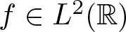 $f \in {L^2}({\mathbb{R}})$ by
 \begin{equation*}
(\widetilde S_t f)(x) := \exp (g_t(x)) f(x+t), \quad x \in {\mathbb{R}},
\end{equation*}
with gt as in (5.1), is bounded with  $\| \widetilde S_t\| \le 1$ and it satisfies the semigroup property (see (i)-(ii) in [Reference Davies14, p. 167]). Furthermore it can be readily verified that the function
 $t \mapsto \widetilde S_t f$ is continuous at t = 0 for each
 $f \in {L^2}({\mathbb{R}})$ and hence
 $(\widetilde S_t)_{t \ge 0}$ is a contraction semigroup. Our next step is to show that the generator of
 $(\widetilde S_t)_{t \ge 0}$, which we shall denote by
 $(Z, {\operatorname{Dom}}(Z))$, is in fact −A. We claim that it is enough to prove
 $Z \subset -A$. Note that, since
 $(\widetilde S_t)_{t \ge 0}$ is a contraction semigroup, it follows that
 $1 \in \rho(Z)$ (see [Reference Engel and Nagel20, Thm. II.1.10 (ii)]) and hence
 $1 \in \rho(Z) \cap \rho(-A) \ne \emptyset$ (recall that
 $\sigma(-A) = \emptyset$ by Proposition 2.1). Therefore
 $Z \subset -A$ implies
 $Z = -A$ (see [Reference Engel and Nagel20, Ex. IV.1.21 (5)]).
Let us take  $f \in {\operatorname{Dom}}(Z)$, with
 $g := Z f \in {L^2}({\mathbb{R}})$, and let
 $\phi \in {C_c^{\infty}({\mathbb{R}})}$ be a test function. Then
 \begin{equation}
\langle g, \phi \rangle = \lim_{t \to 0^{+}} \langle t^{-1} (\widetilde S_t f - f), \phi \rangle = \lim_{t \to 0^{+}} \langle f, t^{-1} (\widetilde S_t^* \phi - \phi) \rangle,
\end{equation}
where  $(\widetilde S_t^*)_{t \ge 0}$ denotes the adjoint semigroup. It is not difficult to verify that its action on
 ${L^2}({\mathbb{R}})$ is given by
 \begin{equation*}
(\widetilde S_t^* f)(x) = \exp(g_t(-x)) f(x - t), \quad x \in {\mathbb{R}}.
\end{equation*}
Assuming that  $\operatorname{supp}(\phi) \subset [a, b]$ (with
 $a, b \in {\mathbb{R}}$, a < b) and
 $0 \lt t \lt \delta$ (with arbitrarily small δ > 0), we have
 \begin{equation}
\begin{aligned}
\langle f, t^{-1} (\widetilde S_t^* \phi - \phi) \rangle &= \int_{a}^{b} f(x) \exp(g_t(-x)) \frac{\overline{\phi(x - t) - \phi(x)}}{t} {{\rm d}} x\\
&\quad + \int_{a}^{b} f(x) \frac{\exp(g_t(-x)) - 1}{t} \overline{\phi(x)} {{\rm d}} x.
\end{aligned}
\end{equation}
Noting that  $g_t(\cdot)$ is continuous and
 $\phi(\cdot)$ is continuously differentiable, an application of the dominated convergence theorem yields
 \begin{equation*}
\lim_{t \to 0^{+}} \int_{a}^{b} f(x) \exp(g_t(-x)) \frac{\overline{\phi(x - t) - \phi(x)}}{t} {{\rm d}} x = -\int_{a}^{b} f(x) \overline{\phi'(x)} {{\rm d}} x = \langle f, -\phi' \rangle.
\end{equation*}
Observe furthermore that, applying the fundamental theorem of calculus for integrable functions (see e.g. [Reference Titchmarsh47, Sec. 11.6]) and the dominated convergence theorem to the second term in the right-hand side of (5.4), we find
 \begin{equation*}
\lim_{t \to 0^{+}} \int_{a}^{b} f(x) \frac{\exp(g_t(-x)) - 1}{t} \overline{\phi(x)} {{\rm d}} x = -\int_{a}^{b} f(x) W(x) \overline{\phi(x)} {{\rm d}} x = \langle f, -W \phi \rangle.
\end{equation*}
Returning to (5.3) with these results, we have shown
 \begin{equation*}
\langle g, \phi \rangle = \langle f, -\phi' - W \phi \rangle,
\end{equation*}
with arbitrary  $\phi \in {C_c^{\infty}({\mathbb{R}})}$, which proves that
 $f \in {\operatorname{Dom}}(-A)$ and
 $Z f = g = -A f$, as claimed. This concludes the proof of the statement that −A generates
 $(\widetilde S_t)_{t \ge 0}$. Since a C 0-semigroup is uniquely determined by its generator (see [Reference Davies14, Thm. 6.1.16]), it follows that
 $\widetilde S_t = S_t$ for all
 $t \ge 0$.
It remains to determine  $\| S_t \|$. Note that, for every
 $t \ge 0$, we have that gt is differentiable a.e. in
 ${\mathbb{R}}$ and
 \begin{equation*}
g_t'(x) = W(x) - W(x+t).
\end{equation*}
By Assumption 3.1 (ii), we can find  $x_1 \gt x_0$ such that
 $W(x_1) \gt \| W \chi_{[-x_0, x_0]} \|_{\infty}$. Choosing
 $t_0 \ge 2 x_1$ and recalling Assumption 3.1 (i), it is clear that, for any (fixed)
 $t \ge t_0$, the value
 $x = -t/2$ solves the equation
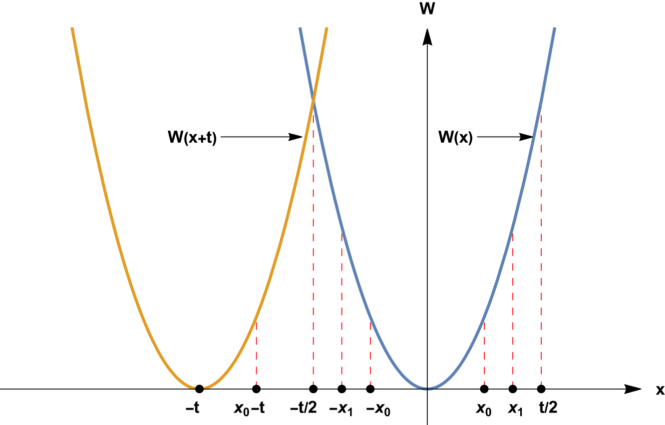
 $g_t'(x) = 0$. We shall show that this solution is unique (the idea of the proof may be best illustrated with a picture: see Fig. 5.1). For this purpose, assume that there exists
 $\hat{x} \in {\mathbb{R}}$ such that
 $g_t'(\hat{x}) = 0$. If
 $\hat{x} \in [0, x_0]$, then
 \begin{equation*}
W(\hat{x}) \le \| W \chi_{[-x_0, x_0]} \|_{\infty} \lt W(x_1) \lt W(t) \le W(\hat{x} + t)
\end{equation*}
Sketch of the solution to  $g_t'(x) = W(x) - W(x+t) = 0$ with fixed
 $t \ge t_0$.

which contradicts the fact that  $\hat{x}$ is a solution. If
 $\hat{x} \in (x_0, +\infty)$, it is not possible to have
 $W(\hat{x}) = W(\hat{x} + t)$ since W(x) is strictly increasing in
 $(x_0, +\infty)$ and t > 0. It therefore follows that
 $\hat{x} \notin [0, +\infty)$. If
 $\hat{x} \le -t \le -2 x_1 \lt -2 x_0$ and
 $\hat{x} + t \lt -x_0$, then
 $\hat{x}$ cannot be a solution because W(x) is strictly decreasing in
 $(-\infty, -x_0)$; on the other hand, if
 $\hat{x} \le -t \le -2 x_1 \lt -x_1$ and
 $\hat{x} + t \in [-x_0, 0]$, we have
 \begin{equation*}
W(\hat{x}) \gt \| W \chi_{[-x_0, x_0]} \|_{\infty} \ge W(\hat{x} + t)
\end{equation*}
and therefore  $\hat{x}$ cannot be a solution in this case either. This shows that
 $\hat{x} \notin (-\infty, -t]$, which leaves us with
 $(-t, 0)$ as the only possible solution domain. Assuming that
 $\hat{x} \in (-t, -t/2)$ and using Assumptions 3.1 (i), (ii), we have
 $W(\hat{x}) \gt W(t/2)$ and
 $W(\hat{x} + t) \lt W(t/2)$, which once again excludes
 $\hat{x}$ being a solution. Finally, if
 $\hat{x} \in (-t/2, 0)$, then
 $W(t/2) \gt W(\hat{x})$ and
 $W(\hat{x} + t) \gt W(t/2)$, contradicting the fact that
 $\hat{x}$ is a solution and completing the proof of the uniqueness of
 $x = -t/2$ as a solution to
 $g_t'(x) = 0$. Since
 $\lim_{|x| \to +\infty} W(x) = +\infty$ by Assumption 3.1 (i)-(ii), it follows that
 $\lim_{|x| \to +\infty} g_t(x) = -\infty$ for any fixed
 $t \ge t_0$. Consequently we can find
 $x_2(t) \gt t/2$ such that
 $g_t(x) \lt g_t(-t/2)$ for all
 $|x| \ge x_2(t)$. But gt is continuous and therefore
 $x = -t/2$ is its maximum in
 $[-x_2(t), x_2(t)]$ and indeed in
 ${\mathbb{R}}$. Hence,
 $\sup_{x \in {\mathbb{R}}} g_t(x) = g_t(-t/2)$ for every
 $t \ge t_0$ and we conclude that
 $\| S_t \| = \exp (g_t(-t/2))$, which proves (5.2).
Remark 5.2. If W is sufficiently regular around 0, e.g.  $W \in C^2({\mathbb{R}})$ and
 $W'(x) \gt 0$, x > 0, then we can take
 $t_0 = 0$ in the statement of Theorem 5.1.
Example 5.3. We estimate the semigroup norm for the instances in Example 3.3 (refer also to Example 4.3).
(i) For
$W(x) = \log \langle x \rangle^{p}$, p > 0, we find
$\int_{0}^{t/2} W(s) {{\rm d}} s = W(t/2) t / 2 - p t / 2 + p \arctan(t/2)$ and hence
\begin{equation*}
\| S_t \| = \langle t/2 \rangle^{- p t} \exp \left(p (t - \pi)\right) (1 + o(1)), \quad t \to +\infty.
\end{equation*}(ii) For
$W(x) = |x|^{p}$, p > 0, we have
$\int_{0}^{t/2} W(s) {{\rm d}} s = (2^{-(p + 1)} / (p + 1)) t^{p + 1}$ and hence
\begin{equation*}
\| S_t \| = \exp \left(-\frac{2^{-p}}{p + 1} t^{p + 1}\right), \quad t \ge 0.
\end{equation*}In the particular case of the complex Airy operator (i.e. p = 2), this yields
$\| S_t \| = \exp(-t^{3} / 12)$, as expected (see [Reference Helffer27, Eq. 14.3.9]).(iii) For the fast-growing function
$W(x) = e^{|x|^{p}}$, p > 0, we have
$\int_{0}^{t/2} W(s) {{\rm d}} s = e^{(t/2)^{p}} F_p(t/2)$, where
$F_p(x)$ represents the generalized Dawson’s integral (see Example 4.3 (iii)). This results in the estimate
\begin{equation*}
\| S_t \| = \exp \left(-\frac{2^{p}}{p} t^{1-p} e^{(\frac{t}{2})^{p}} \left(1 + o(1)\right)\right), \quad t \to +\infty.
\end{equation*}


6. Further remarks
6.1. The level curves of the resolvent
To illustrate the role that generalized Airy operators play in the study of more complex non-self-adjoint operators, we calculate the level curves for the norm of the resolvent of some particular operators analyzed in detail elsewhere ([Reference Arnal and Siegl7], [Reference Arnal4], [Reference Arnal5]).
6.1.1. Schrödinger operators with complex potentials
For  $n \in \mathbb{N}$ consider the m-accretive Schrödinger operator in
 $L^2({\mathbb{R}})$
 \begin{equation}
H_{n} = -\partial_x^2 + i x^{n},
\quad {\operatorname{Dom}}(H_{n}) = W^{2,2}({\mathbb{R}}) \cap {\operatorname{Dom}}(x^{n}),
\end{equation}
and let
 \begin{equation}
A_{n} = -\partial_x + |x|^{n}, \quad
{\operatorname{Dom}}(A_{n}) = W^{1,2}({\mathbb{R}}) \cap {\operatorname{Dom}}(x^{n}),
\end{equation}
be a generalized Airy operator with  $W(x) = |x|^{n}$ as in Example 4.3 (ii).
For an even  $n=2m$, the asymptotic behaviour of the norm of the resolvent of
 $H_{2m}$ for a large positive spectral parameter is found in [Reference Arnal and Siegl7, Ex. 7.1], in detail,
 \begin{equation}
\|(H_{2m}-a)^{-1}\| = \|A_{2m}^{-1}\| (4a)^{-\frac{m}{2m+1}} \left(1+\mathcal{O}(a^{-\frac{m+1}{2m+1}}) \right), \quad a \to +\infty;
\end{equation}
see also [Reference Arnal and Siegl7, Thm. 4.2] for a more general statement including regularly varying potentials V instead of  ${\rm i} x^{2m}$. The claim (6.3) can be extended to curves in
 ${\mathbb{C}}$,
 \begin{equation}
\lambda_a := a + i b(a), \quad a \gt 0, \ b(a) \gt 0,
\end{equation}
adjacent to the positive real axis (see [Reference Arnal5, Sub-sec. 4.3.1.2] or [Reference Arnal and Siegl6, Prop. 5.2] for the proof of a more general statement).
Proposition 6.1. Let  $H_{2m}$ and
 $A_{2m}$,
 $m \in \mathbb{N}$, be as in (6.1) and (6.2), respectively. Suppose that λa in (6.4) is such that for some δ > 0
 \begin{equation}
b(a) a^{-1} + \mu_a^2 \| (A_{2m} - \mu_a)^{-1} \| a^{-\frac{m+1}{2m+1} + \delta}= o(1), \quad a \to +\infty,
\end{equation}
where
 \begin{equation}
\mu_a := (4a)^{-\frac{m}{2m+1}} b(a).
\end{equation}
Then
 \begin{equation}
\| (H_{2m} - \lambda_a)^{-1} \| = \| (A_{2m} - \mu_a)^{-1} \| (4a)^{-\frac{m}{2m+1}} (1 + o(1)), \quad a \to +\infty.
\end{equation}
We now illustrate an application of this proposition to deduce a formula for the  $1/\varepsilon$-level curves of the resolvent norm of
 $H_{2m}$, i.e. the curves λa on which
 $\|(H_{2m}-\lambda_a)^{-1}\|= 1/\varepsilon$ for a given ɛ > 0.
Notice that if b(a) in λa is such that  $\mu_a = \mathcal{O}(1)$ as
 $a \to +\infty$, i.e. if
 \begin{equation}
b(a) = a^{\frac{m}{2m+1}} \mathcal{O}(1), \quad a \to +\infty,
\end{equation}
then the condition (6.5) is satisfied and it follows from (6.7) that
 \begin{equation}
\|(H_{2m}-\lambda_a)^{-1}\| = o(1), \quad a \to + \infty.
\end{equation}
Hence, to find the curves with a constant resolvent norm, b(a) needs to be such that  $\mu_a \to + \infty$ as
 $a \to + \infty$, i.e. we need that
 \begin{equation*}
\limsup_{a \to + \infty} \frac{b(a)}{a^{\frac{m}{2m+1}}} = +\infty.
\end{equation*}
On the other hand, for
 \begin{equation*}
b(a) \gt rsim a^{\frac{m}{2m+1} + \delta}
\end{equation*}
with δ > 0, we have from [Reference Krejčiřík and Siegl33, Ex. 5.3] that
 \begin{equation*}
\|(H_{2m}-\lambda_a)^{-1}\| \to + \infty, \quad a \to + \infty.
\end{equation*}
Thus the sought  $1/\varepsilon$-level curves must be of the form
 $\lambda_a = a + i a^{m/{2m+1}} \varrho(a)$, where ϱ is unbounded, but smaller than any power of a as
 $a \to +\infty$. Combining (6.7) and Example 4.3 (ii) with
 $p = 2m$ we find the following.
Corollary 6.2. Let  $H_{2m}$,
 $m \in \mathbb{N}$, be as in (6.1). For any ɛ > 0, there exists a curve
 $\lambda_a = a + i b(a)$ satisfying
 \begin{equation}
b(a) = \left(\frac{2m + 1}{2m}\right)^{\frac{2m}{2m + 1}} a^\frac{m}{2m + 1} \left(\log \left(
\frac{a^{\frac{m}{2m + 1}}}{\varepsilon}
\right)\right)^{\frac{2m}{2m + 1}}(1+o(1)), \quad a \to + \infty,
\end{equation}
such that, for all sufficiently large a > 0,
 \begin{equation}
\|(H_{2m}-\lambda_a)^{-1}\|= \frac 1\varepsilon.
\end{equation}
Proof. We first verify that the curves with (6.10) satisfy the condition (6.5). To this end, notice that  $\mu_a \to + \infty$ as
 $a \to + \infty$, see (6.6) and (6.10), and Example 4.3 (ii) with
 $p = 2m$ yields
 \begin{equation}
\| (A_{2m} - \mu_a)^{-1} \| = \sqrt{\frac{\pi}{2m}} \mu_a^{\frac{1 - 2m}{4m}} \exp\left(\frac{4m}{2m + 1} \mu_a^{\frac{2m + 1}{2m}}\right) (1 + o(1)), \quad a \to +\infty.
\end{equation}
Straightforward estimates lead to
 \begin{equation*}
b(a) a^{-1} + \mu_a^2 \| (A_{2m} - \mu_a)^{-1} \| a^{-\frac{m+1}{2m+1} + \delta}
\lesssim a^{- \frac{m+1}{2m+1} + \delta'} + a^{- \frac{1}{2m+1} + \delta' + \delta},
\end{equation*}
where  $\delta' \gt 0$ can be taken arbitrarily small. Thus, for δ > 0 sufficiently small, the condition (6.5) indeed holds.
In the next step, we justify formula (6.10). To this end, we write
 \begin{equation}
b(a) = (4a)^\frac{m}{2m+1} x
\end{equation}
and formulate (6.11) as an equation for x > 1; recall that we know that it is necessary that  $x \to + \infty$ as
 $a \to + \infty$, see (6.8) and (6.9). In detail, employing (6.6), (6.7) and (6.12) and taking log in (6.11), the sought x > 1 must satisfy (after straightforward calculations)
 \begin{equation}
x^\frac{2m+1}{2m} = \frac{2m-1}{8m} \log x^\frac{2m+1}{2m} + \frac{2m+1}{4m}\log \frac{a^\frac{m}{2m+1}}{\varepsilon}(1+o(1)), \quad a \to + \infty.
\end{equation}
Notice that the equation (for y) of the form  $y = c \log y + t$ with c > 0 fixed and t > 0 large has exactly one solution y > t and this can be found by iterations
 \begin{equation*}
y_{n+1} = c \log y_n + t, \quad n \in \mathbb{N}_0, \quad y_0:=t,
\end{equation*}
since  $y \mapsto c \log y +t$ is a contraction for
 $y \gt t \geq 2c$. Moreover, by the standard estimates in the fixed point argument, it follows that the solution is of the form
 $y = t(1+o(1))$ as
 $ t \to + \infty$. Applying this for x in (6.14) and returning to (6.13), we find (6.10); the detailed straightforward calculations are omitted.
We conclude by noting that for H 2, i.e. the complex harmonic oscillator first studied by Davies in [Reference Davies15], the curve in (6.10) becomes
 \begin{equation*}
b(a) = \left(\frac32\right)^{\frac23} a^{\frac13} \left(\log(a^{\frac13} \varepsilon^{-1})\right)^{\frac23} (1 + o(1)), \quad a \to +\infty;
\end{equation*}
cf. also [Reference Bordeaux Montrieux13, Sec. 4.2] where a different method is used.
6.1.2. The wave equation with unbounded damping
In a similar way as in Sub-section 6.1.1, generalized Airy operators with non-polynomial potentials a
 \begin{equation}
A = - \partial_x + a(x)
\end{equation}
arise in the analysis of the quadratic operator function  $T(\lambda)$ in
 ${L^2}({\mathbb{R}})$
 \begin{equation}
T(\lambda) = -\partial_x^2 + 2 \lambda a(x) + \lambda^2, \quad \lambda \in {\mathbb{C}} \setminus (-\infty, 0].
\end{equation}
For the relation of  $T(\lambda)$ to the damped wave equation, see e.g. [Reference Arnal4].
For an unbounded, increasing and even a satisfying technical assumptions [Reference Arnal4, Asm. 3.1] (which are stronger than our Assumption 3.1 on  $W:=a$ here), it was established in [Reference Arnal4, Thm. 4.3] that
 \begin{equation}
\| T(i b)^{-1} \| = \| A^{-1} \| (2 b)^{-1} (1 + o(1)), \quad b \to +\infty.
\end{equation}
We note that  $T(\lambda)^* = T(\overline\lambda)$, for
 $\lambda \in {\mathbb{C}} \setminus (-\infty, 0]$, (see [Reference Freitas, Siegl and Tretter21, Thm. 2.4]) and it is therefore sufficient to study λ in the second quadrant of
 ${\mathbb{C}}$.
Similarly as for Schrödinger operators in Sub-section 6.1.1, it is possible to extend the estimate (6.17) to general curves
 \begin{equation}
\lambda_b := -c(b) + i b, \quad b \in {\mathbb{R}}, \ c(b) \geq 0,
\end{equation}
in the left complex half-plane and adjacent to the imaginary axis (a proof of the following proposition can be found in [Reference Arnal5, Sub-sec. 5.2.2]).
Proposition 6.3. Let a satisfy [Reference Arnal4, Asm. 3.1], let  $T(\lambda)$ be as in (6.16) and let A be as in (6.15). Suppose that λb in (6.18) is such that
 \begin{equation}
c(b) b^{-1} + c(b)^2 \| (A - c(b))^{-1} \| b^{-1} = o(1), \quad b \to \infty,
\end{equation}
Then
 \begin{equation}
\| T(\lambda_b)^{-1} \| = \| (A - c(b))^{-1} \| (2 b)^{-1} (1 + o(1)), \quad b \to + \infty.
\end{equation}
Analogously to Corollary 6.2, employing Theorem 4.2, Example 4.3 (i) and (6.20), one can attempt to find  $1/\varepsilon$-level curves of
 $\|T(\cdot)^{-1}\|$ e.g. for
 \begin{equation*}
a(x) = \log \langle x \rangle^p, \quad p \gt 0.
\end{equation*}
We conjecture that, for a given ɛ > 0, there is a curve λb in (6.18) satisfying
 \begin{equation}
c(b) = p \log \log \left(\frac{2b}{\varepsilon}\right)(1+o(1)), \quad b \to + \infty,
\end{equation}
such that, for all sufficiently large b > 0,
 \begin{equation*}
\|T(\lambda_b)^{-1}\| = \frac{1}{\varepsilon}.
\end{equation*}
We note, without elaborating further here, that the issue is that, unlike Corollary 6.2, the curves (6.21) do not satisfy condition (6.19).
6.2. Optimality of resolvent bounds in [Reference Sarıhan and Bandtlow41]
We use Theorem 4.2 to show that the exponential rates in the recent abstract resolvent upper bounds in [Reference Sarıhan and Bandtlow41], generalizing the classical Carleman-type estimates, are optimal (see also [Reference Bandtlow9–Reference Bandtlow and Güven11]). In fact, for quasi-nilpotent operators, they are achieved by the resolvent of generalized Airy operators
 \begin{equation}
A_p = -\partial_x + i|x|^p, \quad {\operatorname{Dom}}(A_p) = W^{1,2}({\mathbb{R}}) \cap {\operatorname{Dom}}(|x|^{p}), \quad p \gt 0.
\end{equation}
In detail, the following is an immediate corollary of [Reference Sarıhan and Bandtlow41, Thm. 4.12] for operators with compact resolvent and empty spectrum.
Corollary 6.4. Let B be a closed operator in a separable Hilbert space  $\mathcal H$ and assume that
 $\sigma(B) = \emptyset$ and
 $B^{-1} \in \mathcal S_{q, \infty}(\mathcal H)$ for some q > 0. Then
 \begin{equation}
\log \|(B-\lambda)^{-1}\| \lesssim |\lambda|^q, \quad |\lambda| \to + \infty.
\end{equation}
Proof. We write the resolvent of B as
 \begin{equation}
(B - \lambda)^{-1} = B^{-1} (I - \lambda B^{-1})^{-1}
\end{equation}
and apply [Reference Sarıhan and Bandtlow41, Thm. 4.12]. Since B −1 is quasi-nilpotent, the upper bound [Reference Sarıhan and Bandtlow41, Eq. 10] (refer also to [Reference Sarıhan and Bandtlow41, Def. 4.8]) reduces to
 \begin{equation*}
\| (I - \lambda B^{-1})^{-1} \| \le F_{\overset{.}{\overline\omega}}(|B^{-1}|_{\overset{.}{\overline\omega}} |\lambda|),
\end{equation*}
where  $w=\{w_k\}$ with
 $w_k := k^{-1/q}$,
 $k \in \mathbb{N}$;
 $\overset{.}{\overline\omega}$ is defined in [Reference Sarıhan and Bandtlow41, Def. 3.11]-[Reference Sarıhan and Bandtlow41, Def. 3.16],
 $F_{\overset{.}{\overline\omega}}$ is defined in [Reference Sarıhan and Bandtlow41, Eq. 8] and
 $|\cdot|_{\overset{.}{\overline\omega}}$ is defined in [Reference Sarıhan and Bandtlow41, Def. 3.2]. By [Reference Sarıhan and Bandtlow41, Prop. 5.4], we finally obtain
 \begin{equation*}
\log F_{\overset{.}{\overline\omega}}(|\lambda|) \lesssim |\lambda|^{q}, \quad |\lambda| \to +\infty,
\end{equation*}
which justifies the claim.
To compare (6.23) with our resolvent estimates for Ap, i.e. for  $\operatorname{Re} \lambda \to + \infty$
 \begin{equation}
\| (A_p - \lambda)^{-1} \| = \sqrt{\frac{\pi}{p}} (\operatorname{Re} \lambda)^{\frac{1 - p}{2 p}} \exp\left(\tfrac{2 p}{p + 1} (\operatorname{Re}\lambda)^{\frac{1 + p}{p}}\right) (1 + o(1)),
\end{equation}
see Theorem 4.2 and Example 4.3 (ii), we analyze the singular values of  $A_p^{-1}$. To this end, a helpful observation used in the proof of Proposition 6.5 is that the graph norm separation (2.2) reduces the question to the well-known eigenvalue asymptotics for the self-adjoint Schrödinger operators in
 $L^2({\mathbb{R}})$
 \begin{equation*}
S_{2p}:=-\partial_x^2 + |x|^{2p}+1, \quad {\operatorname{Dom}}(S_{2p}) = W^{2,2}({\mathbb{R}}) \cap {\operatorname{Dom}}(|x|^{2p}), \quad p \gt 0,
\end{equation*}
for which (see e.g. [Reference Titchmarsh48] or [Reference Titchmarsh49, Sec.7])
 \begin{equation}
S_{2p}^{-1} \in \mathcal S_{r_p,\infty}, \quad r_p := \frac{1 + p}{2p}.
\end{equation}
Proposition 6.5. Let Ap be as in (6.22) in  $L^2({\mathbb{R}})$ and let rp be as in (6.26). Then
 $A_p^{-1} \in \mathcal S_{2r_p,\infty}$, hence by Corollary 6.4,
 \begin{equation}
\log \|(A_p-\lambda)^{-1}\| \lesssim |\lambda|^{\frac{1 + p}{p}}, \quad |\lambda| \to + \infty.
\end{equation}
Comparing (6.25) with (6.27), we conclude that the upper bound (6.27) based on (6.23) and deduced using fairly general operator-theoretic arguments in [Reference Sarıhan and Bandtlow41, Thm. 4.12], yields an optimal rate in the exponential growth of the resolvent norm of Ap.
Proof. It is well-known that the operators  $S_{2p}$ are associated with the closed, symmetric forms
 \begin{equation*}
s_{2p}[u] := \|u'\|^2 + \||x|^p u\|^2+\|u\|^2, \quad {\operatorname{Dom}}(s_{2p}) := W^{1,2}({\mathbb{R}}) \cap {\operatorname{Dom}}(|x|^p),
\end{equation*}
see e.g. [Reference Kato31, Reference Reed and Simon39]. By the graph norm separation (2.2) and the Second Representation Theorem (see [Reference Kato31, Thm. VI.2.23]), we have
 \begin{equation*}
\|A_p u \|^2 + \|u\|^2 \approx \| u' \|^2 + \| |x|^p u \|^2 + \| u \|^2 \approx \| S_{2p}^{\frac12} u \|^2,
\end{equation*}
for any  $u \in {\operatorname{Dom}}(A_p) = {\operatorname{Dom}}(s_{2p}) = {\operatorname{Dom}}(S_{2p}^{\frac12})$. It follows that
 $S_{2p}^{\frac12} A_p^{-1}$ is well-defined and bounded. Hence, writing
 \begin{equation*}
A_p^{-1} = S_{2p}^{-\frac12} S_{2p}^{\frac12} A_p^{-1}
\end{equation*}
and using (6.26) together with the functional calculus (i.e.  $S_{2p}^{-\frac12} \in \mathcal S_{2r_p,\infty}$), we obtain from the standard inequalities for singular values (see e.g. [Reference Gohberg and Krein22, Chap. II §2]) that
 $A_p^{-1} \in \mathcal S_{2r_p,\infty}$ as claimed. The bound (6.27) follows immediately from Corollary 6.4.
6.2.1. Schrödinger operators with imaginary monomial potentials
Finally, although not using the results of this paper, we remark that the upper bounds in [Reference Sarıhan and Bandtlow41, Thm. 4.12] for operators with non-empty spectrum are exhausted by the resolvents of Schrödinger operators Hn in (6.1) for  $n \in \mathbb{N} \setminus \{1\}$ if the spectral parameter remains sufficiently far from the spectrum.
Indeed, arguing as in (6.24), the result [Reference Sarıhan and Bandtlow41, Thm. 4.12] yields that, if  $B^{-1} \in \mathcal S_{q, \infty}$, then for
 $\lambda \to \infty$ such that
 $\operatorname{dist}(1,\sigma(\lambda B^{-1})) \gt rsim 1$ we have
 \begin{equation}
\log \|(B-\lambda)^{-1}\| \lesssim |\lambda|^q, \quad |\lambda| \to + \infty.
\end{equation}
Similarly as for Ap in Proposition 6.5, the graph norm separation for Hn, see e.g. [Reference Bögli, Siegl and Tretter8], leads to
 \begin{equation*}
H_n^{-1} \in \mathcal S_{q_n,\infty}, \quad q_n = \frac{n+2}{2n}, \ n \in \mathbb{N};
\end{equation*}
see also [Reference Almog and Helffer2]. Moreover, we have
 \begin{equation*}
\sigma(H_{3}) \subset {\mathbb{R}}_+, \quad \sigma(H_{2m}) \subset e^{i \frac\pi{2(m+1)}} {\mathbb{R}}_+, \quad m \in \mathbb{N};
\end{equation*}
see [Reference Dorey, Dunning and Tateo18, Reference Shin44] for the case n = 3 and employ complex scaling for  $n = 2m$.
The lower bounds for the resolvent norm are obtained by pseudomode constructions, see [Reference Dencker, Sjöstrand and Zworski16] (or [Reference Krejčiřík, Siegl, Tater and Viola34] with a detailed proof for Schrödinger operators in  $L^2({\mathbb{R}})$) and they yield that
 \begin{equation*}
\log \|(H_n - e^{{\rm i} \theta} s)^{-1}\| \gt rsim s^{q_n} , \quad s \to + \infty,
\end{equation*}
where  $\theta \in (0,\pi/2)$ if n is even,
 $\theta \in (-\pi/2,\pi/2)$ if n is odd. Thus (6.28) are indeed exhausted for Hn.
Acknowledgements
This research was funded in part by the Austrian Science Fund (FWF) 10.55776/P 33568-N. The authors would like to express their gratitude for helpful comments and suggestions from an anonymous referee.