Proof. For a fixed point $x\in Q_\alpha ^k$ with $d(x,G\setminus Q_\alpha ^k)\le \delta ^{-L}\delta ^k$ , we claim that there exists a chain $Q_{\sigma _{k-L+L_0}}^{k-L+L_0}\subset \cdots \subset Q_{\sigma _{k-1}}^{k-1}\subset Q_{\sigma _k}^k=Q_\alpha ^k$ such that $x\in Q_{\sigma _{k-L+L_0}}^{k-L+L_0}$ and

(2.4) $$ \begin{align} d(z_{\sigma_j}^j,z_{\sigma_i}^i)\ge c_0\delta^i/12\quad\text{for all } k-L+L_0\le j< i\le k. \end{align} $$

Indeed, let $x\in Q_\alpha ^k$ , by Proposition 2.2(i)–(iii), for any $n\le k$ , there exists a ‘dyadic cube’ $Q_{\sigma }^n$ such that $x\in Q_{\sigma }^n\subseteq Q_\alpha ^k$ . Hence, there exists a chain $Q_{\sigma _{k-L+L_0}}^{k-L+L_0}\subset \cdots \subset Q_{\sigma _{k-1}}^{k-1}\subset Q_{\sigma _k}^k=Q_\alpha ^k$ with $x\in Q_{\sigma _{k-L+L_0}}^{k-L+L_0}$ . Now, we verify equation (2.4). First, by Proposition 2.2(iv), for every $k-L+L_0\le j\le k$ , we have $x\in B(z_{\sigma _{j}}^j, C_1\delta ^j)$ . We also have $B(z_{\sigma _i}^i,a_0\delta ^i)\subset Q_{\sigma _i}^i\subset Q_\alpha ^k$ . If equation (2.4) were not true, then

$$ \begin{align*} a_0\delta^i&\le d(z_{\sigma_i}^i,G\setminus Q_\alpha^k)\le d(z_{\sigma_i}^i,z_{\sigma_j}^j)+d(z_{\sigma_j}^j,x)\\ &\quad+d(x,G\setminus Q_\alpha^k)< \frac{c_0}{12}\delta^i+C_1\delta^j+\delta^{-L}\delta^k\\ &\le \frac{a_0}{4}\delta^i+\frac{a_0}{3}\delta^{j+1}+\delta^{-L_0}\delta^{i}\le \frac{a_0}{4}\delta^i+\frac{a_0}{3}\delta^{i}+\frac{a_0}{4}\delta^{i}< a_0\delta^i, \end{align*} $$

since $a_0=c_0/3$ , $C_1=2C_0$ , $3C_1\le a_0\delta $ and $\delta ^{-L_0}\le \delta ^{-\log _\delta (12/c_0)}=c_0/12$ . This leads to a contradiction and the claim is proved.

For every ‘dyadic cube’ $Q_\beta ^m$ , we denote it briefly by $(m,\beta )$ . Let $E=\{x\in Q_\alpha ^k:d(x,G\setminus Q_\alpha ^k)\le \delta ^{-L}\delta ^k\}$ . For each $x\in E$ , there exists a chain of pair $(i,\beta (i,x))$ with the properties proved in the first paragraph. Set $S_i=\bigcup _{x\in E}\{z_{\beta (i,x)}^i\}$ for $k-L+L_0\le i\le k$ . In the following, we abbreviate $z^i_{\beta (i,x)}$ to $z_{i(x)}$ . We have the following observation: for $z_{i(x)}\neq z_{j(y)}$ ,

(2.5) $$ \begin{align} &B(z_{i(x)},c_0\delta^i/36)\cap B(z_{j(y)},c_0\delta^j/36)=\emptyset\nonumber\\ &\qquad\text{for all }~z_{i(x)}\in S_i,~z_{j(y)}\in S_j,~k-L+L_0\le i,j\le k. \end{align} $$

For $i=j$ , by equation (2.2), the above assertion is trivially right. For $i\neq j$ , without loss of generality, we assume $i>j$ . Note that by the definition of $S_j$ , for each $z_{j(y)}\in S_j$ , there exists a point $\zeta \in E$ such that $d(z_{j(y)},G\setminus Q_\alpha ^k)\le d(z_{j(y)},\zeta )+d(\zeta ,G\setminus Q_\alpha ^k)\le C_1\delta ^j+\delta ^{-L}\delta ^k$ . It follows that if $B(z_{i(x)},c_0\delta ^i/36)\cap B(z_{j(y)},c_0\delta ^j/36)\neq \emptyset $ , then there exists a point $z\in B(z_{i(x)},c_0\delta ^i/36)\cap B(z_{j(y)},c_0\delta ^j/36)$ such that

$$ \begin{align*} a_0\delta^i&\le d(z_{i(x)},G\setminus Q_\alpha^k)\le d(z_{i(x)},z_{j(y)})+d(z_{j(y)},G\setminus Q_\alpha^k)\\ &\le d(z_{i(x)},z)+d(z_{j(y)},z)+d(z_{j(y)},G\setminus Q_\alpha^k)\\ &\le \frac{c_0}{36}\delta^i+\frac{c_0}{36}\delta^j+C_1\delta^j+\delta^{-L}\delta^k\le \frac{c_0}{18}\delta^i+C_1\delta^j+\delta^{-L}\delta^k\le \frac{a_0}{6}\delta^i+\frac{a_0}{3}\delta^{j+1}+\delta^{-L_0}\delta^{i}\\ &\le \frac{a_0}{6}\delta^i+\frac{a_0}{3}\delta^{i}+\frac{a_0}{4}\delta^{i}< a_0\delta^i, \end{align*} $$

where we used $a_0=c_0/3$ , $C_1=2C_0$ , $3C_1\le a_0\delta $ and $\delta ^{-L_0}\le \delta ^{-\log _\delta (12/c_0)}=c_0/12$ again. This leads to a contradiction and so equation (2.5) holds.

We now prove the desired result. In the following, we write $z_i$ for $z_{i(x)}$ . Setting $G_i=\bigcup _{z_{i}\in S_i}B(z_{i},c_0\delta ^i/36)$ , for any $k-L+L_0\le i\le k$ , we have

$$ \begin{align*} m(E)&\le\sum_{z_{k-L+L_0}\in S_{k-L+L_0}}m(B(z_{k-L+L_0}, C_1\delta^{k-L+L_0}))\\ &\le (K+1)\bigg(\frac{36C_1}{c_0}\bigg)^\epsilon\sum_{z_{k-L+L_0}\in S_{k-L+L_0}}m(B(z_{k-L+L_0},c_0\delta^{k-L+L_0}/36))\\ &=(K+1)\bigg(\frac{36C_1}{c_0}\bigg)^\epsilon\sum_{w_i\in S_i}\sum_{\substack{z_{k-L+L_0}\preceq w_i,\\ z_{k-L+L_0}\in S_{k-L+L_0}}}m(B(z_{k-L+L_0},c_0\delta^{k-L+L_0}/36))\\ &\le (K+1)\bigg(\frac{36C_1}{c_0}\bigg)^\epsilon\sum_{w_i\in S_i}m(B(w_i,C_1\delta^i))\\ &\le(K+1)^2\bigg(\frac{36C_1}{c_0}\bigg)^{2\epsilon} \sum_{w_i\in S_i}m(B(w_i,c_0\delta^i/36))=(K+1)^2\bigg(\frac{72C_0}{c_0}\bigg)^{2\epsilon}m(G_i), \end{align*} $$

where $z_{k-L+L_0}\preceq w_i$ in the third line means that the inclusion of the corresponding ‘dyadic cubes’ $Q_{\beta (k-L+L_0)}^{k-L+L_0}\subset Q^i_{\beta (i)}$ , and we used equation (2.1) in the second and last inequalities since $\delta ^i\ge \delta ^{k-L+L_0}\ge \delta ^{L_1}> 36r_0/c_0$ . The equality in the third line follows from equation (2.5), as does the equality in the last line. From the above inequalities and the disjointness of the sets $G_i$ , we obtain

$$ \begin{align*} m(E)\le \frac{(K+1)^2}{(L-L_0+1)}\bigg(\frac{72C_0}{c_0}\bigg)^{2\epsilon}\sum_{i=k-L+L_0}^km(G_i)\le \frac{(K+1)^2}{(L-L_0+1)}\bigg(\frac{72C_0}{c_0}\bigg)^{2\epsilon}m(Q_\alpha^k), \end{align*} $$

and the lemma follows.

Proof. Let us focus on the first inequality. Let $\ell \in \mathbb {N}$ and set

$$ \begin{align*} E_{-\ell}(Q_\alpha^k)=\{Q_\beta^{k-\ell}\subset Q_\alpha^k:d(Q_\beta^{k-\ell},G\setminus Q_\alpha^{k})\le (C_1+1)\delta^{k-\ell}\}, \end{align*} $$

where $d(Q_\beta ^{k-\ell },G\setminus Q_\alpha ^{k})=\inf _{x\in Q_\beta ^{k-\ell }}d(x,G\setminus Q_\alpha ^{k})$ . We denote by

$$ \begin{align*} e_{-\ell}(Q_\alpha^k)=\{x:x\in Q_\beta^{k-\ell}~\text{with}~Q_\beta^{k-\ell}\in E_{-\ell}(Q_\alpha^k)\} \end{align*} $$

the underlying point set. We proceed to show that

(2.6) $$ \begin{align} \{x\in Q_\alpha^k:d(x,G\setminus Q_\alpha^k)\le \delta^{k-\ell}\}\subseteq e_{-\ell}(Q_\alpha^k)\subseteq\{x\in Q_\alpha^k:d(x,G\setminus Q_\alpha^k)\le\delta^{k-\ell+L_2}\}. \end{align} $$

Fix $x\in Q_\alpha ^k$ such that $d(x,G\setminus Q_\alpha ^k)\le \delta ^{k-\ell }$ . There exists ‘dyadic cube’ $Q_{\beta }^{k-\ell }$ such that $x\in Q_{\beta }^{k-\ell }\subset Q_\alpha ^k$ , and then

$$ \begin{align*} d(Q_{\beta}^{k-\ell},G\setminus Q_\alpha^k)&\le C_1\delta^{k-\ell}+d(x,G\setminus Q_\alpha^k)\le(C_1+1)\delta^{k-\ell}. \end{align*} $$

However, fix a point $x\in e_{-\ell }(Q_\alpha ^k)$ . Then there exists $ Q_\beta ^{k-\ell }\in E_{-\ell }(Q_\alpha ^k)$ such that

$$ \begin{align*} d(x,G\setminus Q_\alpha^k)\le C_1\delta^{k-\ell}+d(Q_\beta^{k-\ell},G\setminus Q_\alpha^k)\le (2C_1+1)\delta^{k-\ell}\le\delta^{k-\ell+L_2}, \end{align*} $$

since $C_1=2C_0$ , and equation (2.6) is proved.

To achieve our goal, we split L into two cases: $L_0<L\le 2L_3$ and $L>2L_3$ . We first prove the case $L>2L_3$ . Set $M_0=[L/L_3]$ ; here and below, $[t]$ denotes the integer part of a real number t. Let $F_1(Q_\alpha ^k)= E_{-L_3}(Q_\alpha ^k)$ and

$$ \begin{align*} F_{n}(Q_\alpha^k)=\bigcup_{Q_\beta^{k-(n-1)L_3}\in F_{n-1}(Q_\alpha^k)}E_{-L_3}(Q_\beta^{k-(n-1)L_3}) \end{align*} $$

for $2\le n\le M_0$ . Let $f_n(Q_\alpha ^k)$ be the underlying point set. It is easy to check that

(2.7) $$ \begin{align} e_{-nL_3}(Q_\alpha^k)\subset f_n(Q_\alpha^k). \end{align} $$

Moreover, for each $Q_\beta ^{k-(n-1)L_3}\in F_{n-1}(Q_\alpha ^k)$ and $1\le n\le M_0$ , plugging equation (2.6) into Lemma 2.5, we obtain

$$ \begin{align*} m(e_{-L_3}(Q_\beta^{k-(n-1)L_3}))&\le m\{x\in Q_\beta^{k-(n-1)L_3}:d(x,G\setminus Q_\beta^{k-(n-1)L_3})\le\delta^{k-nL_3+L_2}\}\\ &\le\frac{(K+1)^2}{(L_3-L_2-L_0+1)} \bigg(\frac{72C_0}{c_0}\bigg)^{2\epsilon}m(Q_\beta^{k-(n-1)L_3})\!\le\frac{1}{2}m(Q_\beta^{k-(n-1)L_3}), \end{align*} $$

since $nL_3\le L<k+L_0-L_1$ . Then,

$$ \begin{align*} m(f_n(Q_\alpha^k))\le \tfrac{1}{2}m(f_{n-1}(Q_\alpha^k)), \end{align*} $$

and iterating the above inequality, we have $m(f_{M_0}(Q_\alpha ^k))\le 2^{-M_0}m(Q_\alpha ^k)$ . From this inequality and equation (2.7), one has

$$ \begin{align*} m(\{x\in Q_\alpha^k:&d(x,G\setminus Q_\alpha^k)\le \delta^{k-L}\})\le m(e_{-L}(Q_\alpha^k))\le m(e_{-M_0L_3}(Q_\alpha^k))\\ &\le m(f_{M_0}(Q_\alpha^k))\le 2^{-M_0}m(Q_\alpha^k)\le 2^{-L/L_3+1}m(Q_\alpha^k)=2\delta^{-\eta L}m(Q_\alpha^k), \end{align*} $$

where the second inequality in the first line follows from the definition of $e_{-\ell }(Q_\alpha ^k)$ .

For the case $L_0<L\le 2L_3$ , using Lemma 2.5 again, we have

$$ \begin{align*} m(\{x\in Q_\alpha^k:d(x,G\setminus Q_\alpha^k)\le \delta^{k-L}\})&\le(K+1)^2\bigg(\frac{72C_0}{c_0}\bigg)^{2\epsilon}m(Q_\alpha^k)\\ &\le \delta^{-\eta L}\delta^{2\eta L_3}(K+1)^2\bigg(\frac{72C_0}{c_0}\bigg)^{2\epsilon}m(Q_\alpha^k)\\ &=4(K+1)^2\bigg(\frac{72C_0}{c_0}\bigg)^{2\epsilon}\delta^{-\eta L}m(Q_\alpha^k). \end{align*} $$

We now prove the second inequality. Let $\widetilde {E}=\{x\in G\setminus Q_\alpha ^k:d(x,Q_\alpha ^k)\le \delta ^{k-L}\}$ . Define the set $\widetilde {I}=\{\beta : Q_\beta ^k\cap \widetilde {E}\neq \emptyset ,\beta \in I_k\}$ and $e(Q_\beta ^k)=\{x\in Q_\beta ^k:d(x,G\setminus Q_\beta ^k)\le \delta ^{k-L}\}$ . Then, by Proposition 2.2(i), we obtain $\widetilde {E}=\bigcup _{\beta \in \widetilde {I}}e(Q_\beta ^k)$ .

Fix $\beta \in \widetilde {I}$ . There exists a point $y_0\in Q_\beta ^k\cap \widetilde {E}$ . By Proposition 2.2(iv), for every $y\in Q_\beta ^k$ , we have

$$ \begin{align*}d(y,z_\alpha^k)\le d(y,y_0)+d(y_0,z_\alpha^k)\le C_1\delta^k+\delta^{k-L}+C_1\delta^k\le 3C_1\delta^k.\end{align*} $$

Hence, $Q_\beta ^k\subseteq B(z_\alpha ^k,3C_1\delta ^k)$ . By Proposition 2.2(ii), the ‘dyadic cubes’ $Q_\beta ^k$ are disjoint; hence, $\bigcup _{\beta \in \widetilde {I}}Q_\beta ^k\subseteq B(z_\alpha ^k,3C_1\delta ^k)$ . Then, by the first inequality and equation (2.1), we obtain

$$ \begin{align*} m(\widetilde{E})&\le m\bigg(\bigcup_{\beta\in\widetilde{I}}e(Q_\beta^k)\bigg)\le \sum_{\beta\in\widetilde{I}}m(e(Q_\beta^k))\\ &\le \sum_{\beta\in\widetilde{I}}C_2\delta^{-L\eta}m(Q_\beta^k)\le C_2\delta^{-L\eta}m\bigg(\bigcup_{\beta\in\widetilde{I}}Q_\beta^k\bigg)\le C_2\delta^{-L\eta}m(B(z_\alpha^k,3C_1\delta^k))\\ &\le C_2(K+1)(3C_1/a_0)^{\epsilon}m(B(z_\alpha^k,a_0\delta^k))\\ &\le C_2(K+1)(3C_1/a_0)^{\epsilon}m(Q_\alpha^k), \end{align*} $$

which completes the proof.

Proof. We check at once that for every $x\in \mathcal {H}(B_{\delta ^{n}},Q^{n+k}_\alpha )$ , the distance $d(x, (Q^{n+k}_\alpha )^{c})$ is not bigger than $\delta ^{n}$ , and so

$$ \begin{align*} \begin{aligned} \mathcal{H}(B_{\delta^{n}},Q^{n+k}_\alpha) &\subseteq \{x\in Q_\alpha^{n+k}:d(x,G\setminus Q_\alpha^{n+k})\le \delta^{n}\}. \end{aligned} \end{align*} $$

Note that $k>L_0$ and $n>L_1-L_0$ , then by Lemma 2.6, we obtain

$$ \begin{align*} \begin{aligned} m(\mathcal{H}(B_{\delta^{n}},Q^{n+k}_\alpha))\le m(\{x\in Q_\alpha^{n+k}:d(x,G\setminus Q_\alpha^{n+k})\le \delta^{n+k-k}\})\le C_2\delta^{-k\eta} m(Q^{n+k}_\alpha), \end{aligned} \end{align*} $$

which is the desired conclusion.

Proof. We only need to estimate the part $m(B(x, r))-m(B(x,r-s))$ , since by the $(\epsilon ,r_0)$ -annular decay property—equation (1.2)—we have $m(B(x, r+s))-m(B(x,r))\le K(s/r)^{\epsilon }m(B(x,r))$ . In the following, we split the s into two cases $s\in (0,r/2)$ and $s\in [r/2,r)$ . For $s\in (0,r/2)$ , since $r\ge 2r_0$ , then $r-s>r/2\ge r_0$ , and applying the $(\epsilon ,r_0)$ -annular decay property again, we have

$$ \begin{align*} m(B(x, r))-m(B(x,r-s))&\le K\bigg(\frac{s}{r-s}\bigg)^{\epsilon}m(B(x,r-s))\\ &\le K\bigg(\frac{r}{r-s}\bigg)^{\epsilon}\bigg(\frac{s}{r}\bigg)^{\epsilon}m(B(x,r))\le K2^{\epsilon}\bigg(\frac{s}{r}\bigg)^{\epsilon}m(B(x,r)). \end{align*} $$

For $s{\kern-1pt}\in{\kern-1pt} [r/2,r)$ , since $1/2{\kern-1pt}\le{\kern-1pt} s/r{\kern-1pt}<{\kern-1pt}1$ , so 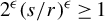$ 2^\epsilon (s/r)^{\epsilon }{\kern-1pt}\ge{\kern-1pt} 1$ and $ m(B(x, r)) {\kern-1pt}-{\kern-1pt} m(B(x,r{\kern-1pt}-{\kern-1pt}s)) \le 2^\epsilon (s/r)^{\epsilon }m(B(x, r))$ . Combining the two cases, we obtain

$$ \begin{align*} m(B(x, r+s))-m(B(x,r-s))\le ((2^\epsilon+1)K+2^\epsilon)\bigg(\frac{s}{r}\bigg)^{\epsilon}m(B(x,r)), \end{align*} $$

and the lemma follows.

Proof. Note that for $k<k_1$ and $r\in [\delta ^n,\delta ^{n+1}]$ , ${\mathcal {I}}(B(x,r),n+k)$ is contained in the annulus $B(x,r+C_1\delta ^{n+k})\setminus B(x,r-C_1\delta ^{n+k})$ . For every $n>n_1$ and $r\in [\delta ^{n},\delta ^{n+1}]$ , Lemma 2.9 yields

$$ \begin{align*} \begin{aligned} m({\mathcal{I}}(B(x,r),n+k))&\le m(B(x,r+C_1\delta^{n+k})\setminus B(x,r-C_1\delta^{n+k}))\\ &\le K_\epsilon\bigg(\frac{C_1\delta^{n+k}}{r}\bigg)^{\epsilon}m(B(x,r))\\ &\le K_\epsilon C_1^\epsilon\delta^{\epsilon k}m(B(x,r)), \end{aligned} \end{align*} $$

which is the desired conclusion.

Proof. For $p=\infty $ , using Lemma 2.10, the conclusion is obvious. For $p\in [1,\infty )$ , fix ${x\in G}$ and note that ${\mathcal {I}}(B(x,r),n+k)\subseteq B(x,r+C_1\delta ^{n+k})$ . Then, using the Hölder inequality and Lemma 2.10, we obtain

$$ \begin{align*} \begin{aligned} {M}_{n+k}f(x)&\le \sup_{r\in[\delta^n,\delta^{n+1}]}\frac{m({\mathcal{I}}(B(x,r),n+k))^{1/p^{\prime}}}{m(B(x,r))} \bigg(\int_{{\mathcal{I}}(B(x,r),n+k)} |f(y)|^pdm(y)\bigg)^{1/p}\\ &\le (K_\epsilon C_1^\epsilon)^{1/p^{\prime}}\delta^{\epsilon k/p^{\prime}}\bigg(\frac{1}{m(B(x,\delta^n))}\int_{B(x,\delta^{n+1}+C_1\delta^{n+k})}|f(y)|^pdm(y)\bigg)^{1/p}, \end{aligned} \end{align*} $$

and by inequality (2.1), the above inequality yields

$$ \begin{align*} &{M}_{n+k}f(x)\\&\quad\le (K_\epsilon C_1^\epsilon)^{1/p^{\prime}}\delta^{\epsilon k/p^{\prime}}\bigg(\frac{(K+1)(\delta+1)^\epsilon}{m(B(x,\delta^{n+1}+C_1\delta^{n+k}))}\int_{B(x,\delta^{n+1}+C_1\delta^{n+k})}|f(y)|^p\,dm(y)\bigg)^{1/p}. \end{align*} $$

Then, applying Proposition 2.11, we have

$$ \begin{align*} \|{M}_{n+k}f\|_{L^{p}}\le((K+1)(\delta+1)^\epsilon)^{1/p}D^{1/p}(K_\epsilon C_1^\epsilon)^{1/p^{\prime}}\delta^{\epsilon k/p^{\prime}}\|f\|_{L^p} \end{align*} $$

and the lemma follows.

Proof. Let $x\in G$ . Fixing $\delta ^n\le r_{i-1}<r_i\le \delta ^{n+1}$ , by the Cauchy–Schwarz inequality and Lemma 2.10, we have

$$ \begin{align*} &\bigg|\frac{1}{m(B(x,r_{i}))}\int_{\mathcal{I}(B(x,r_i)\setminus B(x,r_{i-1}),n+k)}f(y)\,dm(y)\bigg|^2\\&\quad\le \frac{m(\mathcal{I}(B(x,r_{i})\setminus B(x,r_{i-1}),n+k))}{m(B(x,r_{i}))^2}\int_{\mathcal{I}(B(x,r_i)\setminus B(x,r_{i-1}),n+k)}|f(y)|^2\,dm(y)\\&\quad\le \frac{2C_1^\epsilon K_\epsilon\delta^{\epsilon k}}{m(B(x,\delta^{n}))} \int_{\mathcal{I}(B(x,r_i)\setminus B(x,r_{i-1}),n+k)}|f(y)|^2\,dm(y), \end{align*} $$

where we used the fact that $\mathcal {I}(B(x,r_i)\setminus B(x,r_{i-1}),n+k)\subseteq \mathcal {I}(B(x,r_i),n+k)\cup \mathcal {I}(B(x,r_{i-1}),n+k)$ in the last inequality. From this, inequality (2.1) and the observation that $\bigcup _{i}\mathcal {I}(B(x,r_i)\setminus B(x,r_{i-1}),n+k)\subseteq B(x,\delta ^{n+1})$ , it follows that

$$ \begin{align*} M^S_{n+k}f(x)&\le \bigg(\frac{2C_1^\epsilon K_\epsilon\delta^{\epsilon k}}{m(B(x,\delta^{n}))} \int_{B(x,\delta^{n+1})}|f(y)|^2\,dm(y)\bigg)^{1/2}\\ &\le \bigg(\frac{2(K+1)\delta^\epsilon C_1^\epsilon K_\epsilon\delta^{\epsilon k}}{m(B(x,\delta^{n+1}))} \int_{B(x,\delta^{n+1})}|f(y)|^2\,dm(y)\bigg)^{1/2}. \end{align*} $$

Then, using Proposition 2.11, we conclude

$$ \begin{align*} \|M^{S}_{n+k}f\|_{L^2} \le(2(K+1)D\delta^\epsilon C_1^\epsilon K_\epsilon)^{1/2}\delta^{\epsilon k/2}\|f\|_{L^p}.\\[-39pt] \end{align*} $$

Proof of equation (1.8) in the case where $p=2$

Fix $f\in L^2(G,m)$ . Recall that

$$ \begin{align*}S(f)=\bigg(\sum_{n>n_{r_0}}|A^{\prime}_{\delta^n}f-\mathbb{E}_nf|^2\bigg)^{1/2}.\end{align*} $$

Set $n_2=\max \{n_0,n_1,n_{r_0}\}$ . By Lemma 2.14, we first have

$$ \begin{align*} \bigg\|\bigg(\sum_{n_{r_0}<n\le n_2}|A^{\prime}_{\delta^n}f-\mathbb{E}_nf|^2\bigg)^{1/2}\bigg\|_{L^2}\le 2(n_2-n_{r_0})\|f\|_{L^2}. \end{align*} $$

Note that $f=\sum _{n\in \mathbb {Z}}\mathbb {D}_{n}f$ . Set $T_n=A^{\prime }_{\delta ^n}-\mathbb {E}_n$ , $u_n=v_n=\mathbb {D}_{n}f$ , $N=n_2$ in Lemma 2.15; it suffices for our purposes to prove that for every $n>n_2$ and $k\in \mathbb {Z}$ , there exists a sequence $a(k)$ of positive number with $w=\sum _{k\in \mathbb {Z}}a(k)<\infty $ such that

(3.1) $$ \begin{align} \|A^{\prime}_{\delta^n}\mathbb{D}_{n+k}f-\mathbb{E}_n\mathbb{D}_{n+k}f\|_{L^2}\le a(k)\|\mathbb{D}_{n+k}f\|_{L^2}. \end{align} $$

To achieve our goal, we first set

(3.2) $$ \begin{align} k_2=\max\{L_0+1,|k_1|,\min\{k\in\mathbb{N}:a_0\delta^{k-1}>1\}\}, \end{align} $$

and then divide k into three cases $-k_2\le k\leq k_2$ , $k>k_2$ and $k<-k_2$ .

Case $-k_2\le k\le k_2$ . Applying Lemma 2.14 for function $\mathbb {D}_{n+k}f$ , we obtain

$$ \begin{align*} \|A^{\prime}_{\delta^n}\mathbb{D}_{n+k}f-\mathbb{E}_n\mathbb{D}_{n+k}f\|_{L^2}\le {(D^{1/2}+1)}\|\mathbb{D}_{n+k}f\|_{L^2}. \end{align*} $$

Case $k>k_2$ . Note that $\mathbb {E}_n\mathbb {D}_{n+k}f=\mathbb {D}_{n+k}f$ , so we write

$$ \begin{align*} \|A^{\prime}_{\delta^n}\mathbb{D}_{n+k}f-\mathbb{E}_n\mathbb{D}_{n+k}f\|^2_{L^2(G,m)} =\sum_\alpha\int_{Q_\alpha^{n+k-1}}|A^{\prime}_{\delta^n}\mathbb{D}_{n+k}f(x)-\mathbb{D}_{n+k}f(x)|^2\,dm(x). \end{align*} $$

Fix a ‘dyadic cube’ $Q^{n+k-1}_\alpha $ . Note that $\mathbb {D}_{n+k}f(x)$ is a constant valued function on $Q^{n+k-1}_\alpha $ , and so it follows that on $Q^{n+k-1}_\alpha $ , $A^{\prime }_{\delta ^n}\mathbb {D}_{n+k}f(x)-\mathbb {D}_{n+k}f(x)\neq 0$ only if x belongs to the set $\mathcal {H}(B_{\delta ^n},Q^{n+k-1}_\alpha )$ . Applying Lemma 2.7, we have

(3.3) $$ \begin{align} m(\mathcal{H}(B_{\delta^n},Q^{n+k-1}_\alpha))\le C_2\delta^{(1-k)\eta} m(Q^{n+k-1}_\alpha). \end{align} $$

Let $x\in \mathcal {H}(B_{\delta ^n},Q^{n+k-1}_\alpha )$ and define the set $I_{x}=\{\beta :B(x,\delta ^n)\cap Q_{\beta }^{n+k-1}\neq \emptyset \}$ . Set $I_{\alpha }=\bigcup _{x\in \mathcal {H}(B_{\delta ^n},Q^{n+k-1}_\alpha )}I_x$ . Fix $\beta \in I_{\alpha }$ , so there exist a point $x\in \mathcal {H}(B_{\delta ^n},Q^{n+k-1}_\alpha )$ and $y_0\in Q_{\beta }^{n+k-1}$ such that $y_0\in B(x,\delta ^n)\cap Q_{\beta }^{n+k-1}$ . Then, for every $y\in Q_{\beta }^{n+k-1}$ , by Proposition 2.2(iv), we have

$$ \begin{align*} d(y, z_{\alpha}^{n+k-1})\le d(y,y_0)+d(y_0, x)+d(x,z_{\alpha}^{n+k-1})\le 3C_1\delta^{n+k-1}+\delta^n. \end{align*} $$

It follows that for every $\beta \in I_{\alpha }$ , $Q_\beta ^{n+k-1}\subseteq B(z_{\alpha }^{n+k-1},3C_1\delta ^{n+k-1}+\delta ^n))$ and $Q_\alpha ^{n+k-1}\subseteq B(z_{\beta }^{n+k-1},3C_1\delta ^{n+k-1}+\delta ^n))$ . By Proposition 2.2(ii), the ‘dyadic cubes’ $Q_\beta ^k$ are disjoint, and hence $\bigcup _{\beta \in I_{\alpha }}Q_\beta ^{n+k-1}\subseteq B(z_\alpha ^k,3C_1\delta ^{n+k-1}+\delta ^n)$ . Moreover, it is clear that if $\beta \notin I_{\alpha }$ , then $\alpha \notin I_{\beta }$ . However, by Proposition 2.1, one can see that ${B(z_{\alpha }^{n+k-1},3C_1\delta ^{n+k-1}+\delta ^n))}$ is covered by at most $D^{\log _2[(3C_1+1)/a_0]+1}$ balls of radius $a_0\delta ^{n+k-1}$ . Since by Proposition 2.2(iv), we know that each $Q_{\beta }^{n+k-1}$ contains a ball $B(z^{n+k-1}_\beta ,a_0\delta ^{n+k-1})$ , then

(3.4) $$ \begin{align} \#\{I_{\alpha}\}\le D^{\log_2[(3C_1+1)/a_0]+1}, \end{align} $$

here and in what follows, $\#\{A\}$ stands for the number of the set A. Set

$$ \begin{align*}m_{\alpha}=\max_{\beta\in I_{\alpha}}|\mathbb{D}_{n+k}f(z_\beta^{n+k-1})|,\end{align*} $$

where $z_\beta ^{n+k-1}$ is the point associated with the corresponding ‘dyadic cube’ $Q_\beta ^{n+k-1}$ . Since $\mathbb {D}_{n+k}f(x)$ is a constant-valued function on $Q_\beta ^{n+k-1}$ , it follows that

(3.5) $$ \begin{align} m_{\alpha}^2\le\sum_{\beta\in I_{\alpha}}\frac{1}{m(Q_\beta^{n+k-1})}\int_{Q_\beta^{n+k-1}}|\mathbb{D}_{n+k}f(x)|^2\,dm(x). \end{align} $$

By the above inequalities, Proposition 2.2(iv), and equations (3.3) and (2.1), we conclude

$$ \begin{align*} \begin{aligned} &\sum_\alpha\int_{Q_\alpha^{n+k-1}}|A^{\prime}_{\delta^n}\mathbb{D}_{n+k}f(x) -\mathbb{D}_{n+k}f(x)|^2\,dm(x)\\ &\quad= \sum_\alpha \int_{\mathcal{H}(B_{\delta^n},Q^{n+k-1}_\alpha)}|A^{\prime}_{\delta^n}\mathbb{D}_{n+k}f(x) -\mathbb{D}_{n+k}f(x)|^2\,dm(x)\\ &\quad\le 4\sum_\alpha m_{\alpha}^2m(\mathcal{H}(B_{\delta^n},Q^{n+k-1}_\alpha))\\ &\quad\le 4C_2\delta^{(1-k)\eta}\sum_\alpha m_{\alpha}^2m(Q^{n+k-1}_\alpha)\\ &\quad\le {4C_2\delta^{(1-k)\eta}\sum_\alpha\sum_{\beta\in I_{\alpha}}\frac{m(Q^{n+k-1}_\alpha)}{m(Q_\beta^{n+k-1})}\int_{Q_\beta^{n+k-1}}|\mathbb{D}_{n+k}f(x)|^2\,dm(x)}\\ &\quad\le {4C_2\delta^{(1-k)\eta}\sum_\alpha\sum_{\beta\in I_{\alpha}}\frac{m(B(z_\beta^{n+k-1},3C_1\delta^{n+k-1}+\delta^n))}{m(B(z_\beta^{n+k-1},a_0\delta^{n+k-1}))} \int_{Q_\beta^{n+k-1}}|\mathbb{D}_{n+k}f(x)|^2\,dm(x)}\\ &\quad\le{4C_2(K+1)({(3C_1+1)}/{a_0})^\epsilon D^{\log_2[(3C_1+1)/a_0]+1}\delta^{(1-k)\eta}\int_{G}|\mathbb{D}_{n+k}f(x)|^2\,dm(x)}. \end{aligned} \end{align*} $$

Case $k<-k_2$ . Since $\mathbb {E}_{n}\mathbb {D}_{n+k}f=0$ and $\int _{Q^{k+n}_\alpha }\mathbb {D}_{n+k}f=0$ for every $Q^{k+n}_\alpha \in \mathcal {F}_{k+n}$ , then, for any $x\in G$ ,

$$ \begin{align*} {|A^{\prime}_{\delta^n}\mathbb{D}_{n+k}f(x)|}&=\bigg|\frac{1}{m(B(x,\delta^n))}\sum_{\alpha}\int_{Q^{k+n}_\alpha\cap B(x,\delta^n)}\mathbb{D}_{n+k}f(y)\,dm(y)\bigg|\\ &=\bigg|\frac{1}{m(B(x,\delta^n))}\int_{\mathcal{I}(B(x,\delta^n),n+k)}\mathbb{D}_{n+k}f(y)\,dm(y)\bigg|\\ &\le M_{n+k}\mathbb{D}_{n+k}f(x). \end{align*} $$

From this and Lemma 2.12, we obtain

$$ \begin{align*} \|A^{\prime}_{\delta^n}\mathbb{D}_{n+k}f\|_{L^2}\le\|M_{n+k}\mathbb{D}_{n+k}f\|_{L^2}\le D_2 \delta^{k\epsilon/2}\|\mathbb{D}_{n+k}f\|_{L^2}. \end{align*} $$

Therefore, for every $n>n_2$ , we determine

$$ \begin{align*} a(k)= \begin{cases} (4C_2(K+1)({(3C_1+1)}/{a_0})^\epsilon D^{\log_2[(3C_1+1)/a_0]+1}\delta^{\eta})^{1/2}\delta^{-\eta k/2}, & k>k_2, \\ D^{1/2}+1, & -k_2\le k\le k_2, \\ D_2\delta^{\epsilon k/2}, & k<-k_2, \end{cases} \end{align*} $$

and $\sum _{k\in \mathbb {Z}}a(k)<\infty $ , which completes the proof.

Proof of equation (1.11) in the case where $p=2$

First, by Lemma 2.14, we have

$$ \begin{align*} \bigg\|\bigg(\sum_{n_{r_0}\le n\le n_2}|SV_n(f)|^2\bigg)^{1/2}\bigg\|_{L^2}\le 2(n_2-n_{r_0}+1)C_4\|f\|_{L^2}. \end{align*} $$

Set $T_n=SV_n$ , $u_n=v_n=\mathbb {D}_{n}$ , $N=n_2$ in Lemma 2.15. For every $n>n_2$ , we divide k into three cases $-k_2\le k\leq k_2$ , $k> k_2$ and $k<-k_2$ , where $k_2$ is defined in equation (3.2).

Case $-k_2\le k\leq k_2$ . For function $\mathbb {D}_{n+k}f$ , using Lemma 2.14 again, we have

$$ \begin{align*} \|V_2(A^{\prime}_{r}\mathbb{D}_{n+k}f:r\in[\delta^{n},\delta^{n+1}))\|_{L^2}\le C_4\|\mathbb{D}_{n+k}f\|_{L^2}. \end{align*} $$

Case $k>k_2$ . We write

$$ \begin{align*} \begin{aligned} \|&V_2(A^{\prime}_{r}\mathbb{D}_{n+k}f:r\in[\delta^{n},\delta^{n+1}))\|^2_{L^2(G,m)}\\ &=\sum_\alpha\int_{Q_\alpha^{n+k-1}}|V_2(A^{\prime}_{r}\mathbb{D}_{n+k}f(x):r\in[\delta^{n},\delta^{n+1}))|^2\,dm(x). \end{aligned} \end{align*} $$

Fix a ‘dyadic cube’ $Q_\alpha ^{n+k-1}$ . Recall that $\mathbb {D}_{n+k}f(x)$ is a constant valued function on $Q_\alpha ^{n+k-1}$ . It follows that for every $\delta ^n\le r_i<r_{i+1}<\delta ^{n+1}$ and $x\in Q_\alpha ^{n+k-1}$ , $|A^{\prime }_{r_{i+1}}\mathbb {D}_{n+k}f(x)-A^{\prime }_{r_i}\mathbb {D}_{n+k}f(x)|\neq 0$ only if there exists at least one ball $B(x,r_i)$ or $B(x,r_{i+1})$ intersecting with $(Q^{n+k-1}_\alpha )^{c}$ . So $V_2(A^{\prime }_{r}\mathbb {D}_{n+k}f:r\in [\delta ^{n},\delta ^{n+1}))$ is supported on $\mathcal {H}(B_{\delta ^{n+1}},Q^{n+k-1}_\alpha )$ . By Lemma 2.7, we have

(3.6) $$ \begin{align} m(\mathcal{H}(B_{\delta^{n+1}},Q^{n+k-1}_\alpha))\le C_2\delta^{(2- k)\eta} m(Q^{n+k-1}_\alpha). \end{align} $$

However, by equation (2.8), we know that $V_2(A^{\prime }_{r}\mathbb {D}_{n+k}f(x):r\in [\delta ^{n},\delta ^{n+1}))$ is controlled by the sum of $SV_I(\mathbb {D}_{n+k}f)(x)$ and $SV_{II}(\mathbb {D}_{n+k}f)(x)$ , where

$$ \begin{align*} &SV_I(\mathbb{D}_{n+k}f)(x)\\&\quad=\bigg(\sup_{\delta^{n}\le r_0<\cdots<r_J<\delta^{n+1}}\sum_{i=1}^J\frac{1}{m(B(x,r_i))^2}\bigg|\!\int_{B(x,r_i)\setminus B(x,r_{i-1})}\mathbb{D}_{n+k}f(y)\,dm(y)\bigg|^2\bigg)^{1/2} \end{align*} $$

and

$$ \begin{align*} \begin{aligned} &SV_{II}(\mathbb{D}_{n+k}f)(x)=\\ &\bigg(\sup_{\delta^{n}\le r_0<\cdots<r_J<\delta^{n+1}}\sum_{i=1}^J \bigg|\bigg(\frac{1}{m(B(x,r_{i-1}))}-\frac{1}{m(B(x,r_i))}\bigg)\!\int_{B(x,r_{i-1})}\mathbb{D}_{n+k}f(y)\,dm(y)\bigg|^2\bigg)^{1/2}. \end{aligned} \end{align*} $$

Let $x\in \mathcal {H}(B_{\delta ^{n+1}},Q^{n+k-1}_\alpha )$ and set $I_{x}=\{\beta :B(x,\delta ^{n+1})\cap Q_{\beta }^{n+k-1}\neq \emptyset \}$ . We define the set $I_\alpha =\bigcup _{x\in \mathcal {H}(B_{\delta ^{n+1}},Q^{n+k-1}_\alpha )}I_x$ . Similar to equation (3.4), we have $\#\{I_{\alpha }\}\le D^{\log _2[(3C_1+1)/a_0]+1}$ . Write

$$ \begin{align*}m_{\alpha}=\max_{\beta\in I_\alpha}|\mathbb{D}_{n+k}f(z_\beta^{n+k-1})|.\end{align*} $$

It follows from equation (2.1) that

$$ \begin{align*} \begin{aligned} &SV_I(\mathbb{D}_{n+k}f)^2(x)\\&\quad\le \frac{m(B(x,\delta^{n+1})\setminus B(x,\delta^{n}))}{m(B(x,\delta^{n}))^2} \sup_{\delta^{n}\le r_0<\cdots<r_J<\delta^{n+1}}\sum_{i=1}^J\!\int_{B(x,r_i)\setminus B(x,r_{i-1})}\! |\mathbb{D}_{n+k}f(y)|^2\,dm(y)\\&\quad\le \bigg(\frac{m(B(x,\delta^{n+1})\setminus B(x,\delta^{n}))}{m(B(x,\delta^{n}))}\bigg)^2m_{\alpha}^2\le (K+1)^2\delta^{2\epsilon} m_{\alpha}^2 \end{aligned} \end{align*} $$

and

$$ \begin{align*} \begin{aligned} &SV_{II}(\mathbb{D}_{n+k}f)^2(x)\\ &\quad\le m_{\alpha}^2m(B(x,\delta^{n+1}))^2 \bigg(\sup_{\delta^{n}\le r_0<\cdots<r_J<\delta^{n+1}}\sum_{i=1}^J \bigg|\frac{1}{m(B(x,r_{i-1}))}-\frac{1}{m(B(x,r_i)))}\bigg|\bigg)^2\\ &\quad\le m_{\alpha}^2m(B(x,\delta^{n+1}))^2\bigg(\frac{1}{m(B(x,\delta^{n}))}-\frac{1}{m(B(x,\delta^{n+1}))}\bigg)^2\le (K+1)^2\delta^{2\epsilon} m_{\alpha}^2. \end{aligned} \end{align*} $$

Combining the above two inequalities with equations (3.5) and (3.6), we have

$$ \begin{align*} &\int_{Q_\alpha^{n+k-1}}|V_2(A^{\prime}_{r}\mathbb{D}_{n+k}f(x):r\in[\delta^{n},\delta^{n+1}))|^2\,dm(x)\\ &\quad=\int_{\mathcal{H}(B_{\delta^{n+1}},Q^{n+k-1}_\alpha)}|V_2(A^{\prime}_{r}\mathbb{D}_{n+k}f(x):r\in[\delta^{n},\delta^{n+1}))|^2\,dm(x)\\ &\quad\le 2\int_{\mathcal{H}(B_{\delta^{n+1}},Q_\alpha^{n+k-1})}SV_I(\mathbb{D}_{n+k}f)^2(x)+SV_{II}(\mathbb{D}_{n+k}f)^2(x)\,dm(x)\\ &\quad\le 4(K+1)^2\delta^{2\epsilon} m(\mathcal{H}(B_{\delta^{n+1}},Q_\alpha^{n+k-1}))m_{\alpha}^2\\ &\quad\le{4C_2(K+1)^2\delta^{2\epsilon}\delta^{(2-k)\eta}\sum_{\beta\in I_{\alpha}}\frac{m(Q_\alpha^{n+k-1})}{m(Q_\beta^{n+k-1})}\int_{Q_{\beta}^{n+k-1}}|\mathbb{D}_{n+k}f(x)|^2\,dm(x)}\\ &\quad\le 4C_2(K+1)^2((3C_1+1)/a_0)^\epsilon \delta^{2\epsilon}\delta^{(2-k)\eta}\sum_{\beta\in I_{\alpha}}\int_{Q_{\beta}^{n+k-1}}|\mathbb{D}_{n+k}f(x)|^2\,dm(x), \end{align*} $$

and summing over all $\alpha $ shows

$$ \begin{align*} &\|V_2(A^{\prime}_{r}\mathbb{D}_{n+k}f:r\in[\delta^{n},\delta^{n+1}))\|_{L^2}\\ &\quad\le (4C_2(K+1)^2((3C_1+1)/a_0)^\epsilon D^{\log_2[(3C_1+1)/a_0]+1}\delta^{2\epsilon}\delta^{(2-k)\eta})^{1/2}\|\mathbb{D}_{n+k}f\|_{L^2}. \end{align*} $$

Case $k<-k_2$ . Let $x\in G$ . Note that for every $\delta ^n\le r_{i-1}<r_i\le \delta ^{n+1}$ ,

$$ \begin{align*} \begin{aligned} &\int_{B(x,r_i))\setminus B(x,r_{i-1})}\mathbb{D}_{n+k}f(y)\,dm(y)=\int_{\mathcal{I}(B(x,r_i))\setminus B(x,r_{i-1}),n+k)}\mathbb{D}_{n+k}f(y)\,dm(y),\\ &\int_{B(x,r_{i-1})}\mathbb{D}_{n+k}f(y)\,dm(y)=\int_{\mathcal{I}(B(x,r_{i-1}),n+k)}\mathbb{D}_{n+k}f(y)\,dm(y), \end{aligned} \end{align*} $$

so $SV_I(\mathbb {D}_{n+k}f)(x)= M^S_{n+k}(\mathbb {D}_{n+k}f)(x)$ . Moreover, using the estimate (2.1) and the fact that the $\ell ^1$ -norm is greater than the $\ell ^2$ -norm, we obtain

$$ \begin{align*} &SV_{II}(\mathbb{D}_{n+k}f)(x)\\&\quad\le\sup_{\delta^{n}\le r_0<\cdots<r_J<\delta^{n+1}}\sum_{i=1}^J \bigg|\bigg(\frac{1}{m(B(x,r_{i-1}))}-\frac{1}{m(B(x,r_i))}\bigg)\\&\qquad\qquad\qquad\quad\qquad\qquad\int_{\mathcal{I}(B(x,r_{i-1}),n+k)}\mathbb{D}_{n+k}f(y)\,dm(y)\bigg|\\&\quad\le (K+1)\delta^\epsilon \sup_{\delta^{n}\le r_0<\cdots<r_J<\delta^{n+1}}\sum_{i=1}^J \bigg|\frac{m(B(x,\delta^{n+1}))}{m(B(x,r_{i-1}))}-\frac{m(B(x,\delta^{n+1}))}{m(B(x,r_i))}\bigg|{M}_{n+k}(\mathbb{D}_{n+k}f)(x)\\& \quad\le (K+1)^2\delta^{2\epsilon}{M}_{n+k}(\mathbb{D}_{n+k}f)(x). \end{align*} $$

Using Lemmas 2.13 and 2.12, we have

$$ \begin{align*} &\|V_2(A^{\prime}_{r}\mathbb{D}_{n+k}f:r\in[\delta^{n},\delta^{n+1}))\|_{L^2}\le\|SV_I(\mathbb{D}_{n+k}f)\|_{L^2}+\|SV_{II}(\mathbb{D}_{n+k}f)\|_{L^2}\\ &\quad\le \|M^S_{n+k}(\mathbb{D}_{n+k}f)\|_{L^2}+(K+1)^2\delta^{2\epsilon}\|{M}_{n+k}(\mathbb{D}_{n+k}f)\|_{L^2}\\ &\quad\le(C_3+ (K+1)^2\delta^{2\epsilon} D_2)\delta^{\epsilon k/2}\|\mathbb{D}_{n+k}f\|_{L^2}. \end{align*} $$

Hence, for every $n>n_2$ , we determine

$$ \begin{align*} &a(k)\\ &\ =\begin{cases} {(4C_2(K+1)^2((3C_1+1)/a_0)^\epsilon D^{\log_2[(3C_1+1)/a_0]+1}\delta^{2(\epsilon+\eta)})^{1/2}\delta^{-k\eta/2}}, & k>k_2, \\ C_4, & -k_2\le k\le k_2, \\ (C_3+ (K+1)^2\delta^{2\epsilon} D_2)\delta^{\epsilon k/2}, &k<-k_2, \end{cases} \end{align*} $$

and $\sum _k a(k)<\infty $ , which completes the proof.

Proof of equation (1.9)

Fix $f\in L^1(G,m)$ and $\gamma>0$ . Keeping the notation in Lemma 4.1, we get $f=g+b+\xi $ . We first have

$$ \begin{align*} m(\{x\in G:S(f)(x)>\gamma\}) &\le m(\{x\in G:S(g)(x)>{\gamma}/{3}\})\\ &\quad+m(\{x\in G:S(b)(x)>{\gamma}/{3}\})\\ &\quad+m(\{x\in G:S(\xi)(x)>{\gamma}/{3}\}). \end{align*} $$

By the $L^2$ -boundedness of the operator S and Lemma 4.1(ii), the first term on the right-hand side is controlled by

$$ \begin{align*} \begin{aligned} m(\{x\in G:S(g)(x)>{\gamma}/{3}\})&\le \frac{9}{\gamma^2}\int_G|S(g)(x)|^2\,dm(x)\le\frac{9c_2}{\gamma^2}\int_G|g(x)|^2\,dm(x)\\ &\le \frac{108\sqrt{6} c_2}{\gamma}\int_G|f(x)|\,dm(x). \end{aligned} \end{align*} $$

It remains to handle the other two terms, we set

where . By equation (2.1) and the fact that $M_d$ is of weak type $(1,1)$ , is controlled by

We now focus on the term . Recall that $n_2=\max \{n_0, n_1\}$ , we decompose

For the first part of the right-hand side of the above inequality, using Lemmas 2.14 and 4.1(iv), we have

For the second part, we first have

(4.1)

We now deal with the integral term . Let

$$ \begin{align*} k_4=\max\{k:k<0~\&~2C_1\delta^{k+1}\le 1\},\quad k_5=\max\{|k_4|,k_3\}. \end{align*} $$

We split the k into three cases: $-k_5\le k\le k_5$ , $k>k_5$ and $k<-k_5$ . We will prove that

where

(4.2) $$ \begin{align} a(k)= \begin{cases} {(D+1)}, & -k_5\le k\le k_5; \\ 0, & k>k_5; \\ {4^{\epsilon}(K+1)^2C_1^\epsilon DK_\epsilon\delta^{\epsilon k}}, & k<-k_5. \end{cases} \end{align} $$

Assume this result momentarily. Combining equations (4.1), (4.2) with Lemma 4.1(iv), one can see immediately that

We now prove equation (4.2).

Case $-k_5\le k\le k_5$ . Using Lemma 2.14 for function $\xi _\alpha ^{n+k}$ , we have

Case $k>k_5$ . Note that $\xi ^{n+k}_\alpha $ is supported on $\widehat {Q}_\alpha ^{n+k}$ . Recall that $\widetilde {Q}_\alpha ^{n+k}=\{y\in G:d(y,z_\alpha ^{n+k})\le 3C_1\delta ^{n+k+1}\}$ . Let $y\in \widehat {Q}_\alpha ^{n+k}$ . We have $d(y,z_\alpha ^{n+k})\le d(y,\widehat {z}_\alpha ^{n+k+1})+d(z_\alpha ^{n+k},\widehat {z}_\alpha ^{n+k+1})\le 2C_1\delta ^{n+k+1}$ . This gives $\widehat {Q}_\alpha ^{n+k}\subseteq \widetilde {Q}_\alpha ^{n+k}$ .

Fix . There exists an unique ‘dyadic cube’ $Q_\beta ^n$ containing x. We claim that

(4.3) $$ \begin{align} B(x,\delta^n)\cap\widehat{Q}_\alpha^{n+k}=\emptyset,~Q_\beta^n\cap\widehat{Q}_\alpha^{n+k}=\emptyset. \end{align} $$

Since

$$ \begin{align*}A^{\prime}_{\delta^n}\xi_\alpha^{n+k}(x)=\frac{1}{m(B(x,r))}\int_{B(x,r)\cap \widehat{Q}_\alpha^{n+k}}\xi_\alpha^{n+k}(y)\,dm(y)\end{align*} $$

and

$$ \begin{align*}\mathbb{E}_n\xi_\alpha^{n+k}(x)=\frac{1}{m(Q_\beta^{n})}\int_{Q_\beta^n\cap\widehat{Q}_\alpha^{n+k}}\xi_\alpha^{n+k}(y)\,dm(y),\end{align*} $$

it follows from the claim that $A^{\prime }_{\delta ^n}\xi _\alpha ^{n+k}=\mathbb {E}_n\xi _\alpha ^{n+k}=0$ .

We now prove the claim. If $Q_\beta ^n\cap \widehat {Q}_\alpha ^{n+k}\neq \emptyset $ , by Proposition 2.2(ii), it follows that $x\in Q_\beta ^n\subseteq \widehat {Q}_\alpha ^{n+k}\subseteq \widetilde {Q}_\alpha ^{n+k}$ , which is a contradiction with . However, if there exists a point $z\in B(x,\delta ^n)\cap \widehat {Q}_\alpha ^{n+k}$ , then $d(x,\widehat {z}_\alpha ^{n+k+1})\le d(x,z)+d(z,\widehat {z}_\alpha ^{n+k+1})\le \delta ^n+C_1\delta ^{n+k+1}< 2C_1\delta ^{n+k+1}$ , and so it follows that

$$ \begin{align*}d(x,z_\alpha^{n+k})\le d(x,\widehat{z}_\alpha^{n+k+1})+d(z_\alpha^{n+k},\widehat{z}_\alpha^{n+k+1})<3C_1\delta^{n+k+1},\end{align*} $$

which is in contrast to , and equation (4.3) is proved. This gives the conclusion.

Case $k<-k_5$ . We also have

Indeed, let $x\in Q_\beta ^{n}$ . If $ Q_\beta ^{n}\cap \widehat {Q}_\alpha ^{n+k}\neq \emptyset $ , then by Proposition 2.2(ii), it follows that $\widehat {Q}_\alpha ^{n+k}\subseteq Q_\beta ^{n}$ and

$$ \begin{align*} \mathbb{E}_n\xi_\alpha^{n+k}(x)=\int_{\widehat{Q}_\alpha^{n+k}}\xi_\alpha^{n+k}(y)\,dm(y)=0. \end{align*} $$

Given a ball $B(x,r)$ and ‘dyadic cube’ $Q_\alpha ^k$ , we define the set $\mathcal {I}(B(x,r),Q^{k}_\alpha )=\{Q_\alpha ^{k}\cap B(x,r): Q_\alpha ^{k}\cap \partial B(x,r) \neq \emptyset \}$ . Since $\xi _\alpha ^{n+k}$ is supported on $\widehat {Q}_\alpha ^{n+k}$ and $\int _{\widehat {Q}_\alpha ^{n+k}}\xi _{\alpha }^{n+k}=0$ , it follows that $\text { for all } x\in G$ ,

$$ \begin{align*} |A_{\delta^n}\xi_{\alpha}^{n+k}(x)|&=\bigg|\frac{1}{m(B(x,\delta^n))}\int_{\mathcal{I}(B(x,\delta^n),\widehat{Q}^{n+k}_\alpha)}\xi_{\alpha}^{n+k}(y)\,dm(y)\bigg|\\ &\le \frac{1}{m(B(x,\delta^n))}\int_{\delta^n-2C_1\delta^{n+k+1}\le d(x,y)\le\delta^n+2C_1\delta^{n+k+1}}|\xi_{\alpha}^{n+k}(y)|\,dm(y). \end{align*} $$

Then, by the above estimate, we obtain

(4.4)

Set $A(y)={B(y,\delta ^n+2C_1\delta ^{n+k+1})\setminus B(y,\delta ^n-2C_1\delta ^{n+k+1})}$ . Fix $y\in G$ . By equation (2.1), we have

By the same argument as in the proof of [Reference Aldaz1, Theorem 3.5], we have the following properties. For any $0<\varepsilon <1$ , there exist M-points $\{u_i:1\le i\le M\}$ with $M\le D$ in $B(y,\delta ^{n}+2C_1\delta ^{n+k+1})$ such that $B(y,\delta ^n+2C_1\delta ^{n+k+1})\setminus \bigcup _{i=1}^M B(u_i,\delta ^n+2C_1\delta ^{n+k+1})=\emptyset $ . Fix $x\in B(y,\delta ^{n}+2C_1\delta ^{n+k+1})$ , and let j be the first index such that

$$ \begin{align*} x\!\in\! B(u_j,\delta^n+2C_1\delta^{n+k+1}),~m(B(u_j,\delta^n+2C_1\delta^{n+k+1}))\!\le\! (1+\varepsilon) m(B(x,\delta^n+2C_1\delta^{n+k+1})). \end{align*} $$

By the above discussions, we first have

(4.5)

Note that each $u_i\in B(y,\delta ^n+2C_1\delta ^{n+k+1})$ , then $B(y,\delta ^n)\subseteq B(u_i,2\delta ^{n}+2C_1\delta ^{n+k+1})$ . It follows from equation (2.1) that

$$ \begin{align*} \frac{m(B(y,\delta^n))}{m(B(u_i,\delta^n+2C_1\delta^{n+k+1}))}\le 2^\epsilon(K+1). \end{align*} $$

Moreover, by Lemma 2.9, we have ${m(A(y))}/{m(B(y,\delta ^n))}\le K_\epsilon C_1^\epsilon \delta ^{\epsilon k}$ . Combining these two estimates with equation (4.5), we conclude

(4.6)

Combining equation (4.6) with equation (4.4), and then letting $\varepsilon \rightarrow 0$ , we obtain $\|A_{\delta ^n}\xi _{\alpha }^{n+k}\|_{L^1}\le 6^{\epsilon }(K+1)^2C_1^\epsilon DK_\epsilon \delta ^{\epsilon k}\|\xi _{\alpha }^{n+k}\|_{L^1}$ . Together with the above three cases for k, equation (4.2) is proved.

The estimate of is similar and so will only be indicated briefly. Fix $n>n_2$ . We first prove that

(4.7)

Note that $b=\sum _{k}\sum _{\alpha \in \Lambda _k}b_\alpha ^k$ . By the linearity of operator $\mathbb {E}_n$ , we only need to prove that for each $b_\alpha ^k$ , $\mathbb {E}_n{b_\alpha ^k}=0$ .

Fix . Let $Q_\beta ^n\ni x$ . Since $b_\alpha ^k$ is supported on $Q_\alpha ^k$ , it follows that $\mathbb {E}_n{b^k_\alpha }(x)=\int _{Q_\alpha ^k\cap Q_\beta ^n}b_\alpha ^k(y)\,dm(y)$ . If $Q_\alpha ^k\cap Q_\beta ^n\neq \emptyset $ , we split k into two cases: $k\ge n$ and $k<n$ . For $k\ge n$ , by Proposition 2.2(ii), it follows that $x\in Q_\beta ^n\subseteq Q_\alpha ^k$ , this leads to a contradiction since . For $k<n$ , using Proposition 2.2(ii) again, we have $Q_\alpha ^k \subseteq Q_\beta ^n$ . It follows immediately that

$$ \begin{align*} \mathbb{E}_n{b^k_\alpha}(x)=\frac{1}{m(Q_\beta^n)}\int_{Q_\alpha^k}b_\alpha^k(y)\,dm(y)=0. \end{align*} $$

This gives equation (4.7). Similar to equation (4.2), we can also establish the following inequality:

(4.8)

Note that for $-k_5\le k\le k_5$ , the estimate holds by Proposition 2.11. For $k>k_5$ , the estimate holds true by equation (4.3) and the fact that $b_\alpha ^{n+k}$ is supported on $Q_\alpha ^{n+k}$ . For $k<-k_5$ , we first have

$$ \begin{align*} |A_{\delta^n}b_{\alpha}^{n+k}(x)|&=\bigg|\frac{1}{m(B(x,\delta^n))}\int_{\mathcal{I}(B(x,\delta^n),{Q}^{n+k}_\alpha)}b_{\alpha}^{n+k}(y)\,dm(y)\bigg|\\ &\le \frac{1}{m(B(x,\delta^n))}\int_{\delta^n-2C_1\delta^{n+k}\le d(x,y)\le\delta^n+2C_1\delta^{n+k}}|b_{\alpha}^{n+k}(y)|\,dm(y). \end{align*} $$

By the same estimates as equations (4.4) and (4.6), the above inequality yields

together with the above two cases, this proves equation (4.8) and the proof is complete.

Proof of equation (1.12)

Fix $f\in L^1(G,m)$ . Decompose $f=g+b+\xi $ . The desired estimate for g is true by the fact that $SV$ is of strong type $(2,2)$ . In what follows, we only state the proof for $\xi $ since the proof for b is similar.

By similar arguments as in the previous proof, we mainly need to prove the following inequality for $n>n_2$ :

where

$$ \begin{align*} a(k)=\begin{cases} C_4, &-k_5\le k\le k_5; \\ 0, &k>k_5; \\ 2\cdot 4^\epsilon (\delta+1)^{2\epsilon} (K+1)^3C_1^\epsilon D K_\epsilon\delta^{\epsilon k}, & k<-k_5. \end{cases} \end{align*} $$

We now focus on the above inequality. Fix $n>n_2$ . Note that for $-k_5\le k\le k_5$ , by Lemma 2.14, the estimate is true. For $k>k_5$ , similar to equation (4.3), we can prove that for every and $r\in [\delta ^n,\delta ^{n+1}]$ , $B(x,r)\cap \widehat {Q}_\alpha ^{n+k}=\emptyset $ ; hence, $V_2(A^{\prime }_{r}\xi ^{n+k}_{\alpha }:r\in [\delta ^{n},\delta ^{n+1}))=0$ . It remains to prove the case $k<-k_5$ .

Given an annular $B(x,R)\setminus B(x,r)$ and ‘dyadic cube’ $Q_\alpha ^k$ , we define the set $\mathcal {I}(B(x,R){\kern-0.5pt}\setminus{\kern-0.5pt} B(x,r),Q^{k}_\alpha ){\kern-1pt}={\kern-1pt}\{Q_\alpha ^{k}{\kern-1pt}\cap{\kern-1pt} (B(x,R){\kern-0.5pt}\setminus{\kern-0.5pt} B(x,r)): Q_\alpha ^{k}{\kern-1pt}\cap{\kern-1pt} \partial (B(x,R){\kern-0.5pt}\setminus{\kern-0.5pt} B(x,r)) {\kern-0.5pt}\neq {\kern-1pt}\emptyset \}$ . Since $\int _{\widehat {Q}_\alpha ^{n+k}}\xi _{\alpha }^{n+k}=0$ , it follows that

$$ \begin{align*} &V_2(A^{\prime}_{r}\xi^{n+k}_{\alpha}(x):r\in[\delta^{n},\delta^{n+1}))\\&\quad \le\sup_{\delta^{n}\le r_0<\cdots<r_J<\delta^{n+1}}\sum_{i=1}^J\frac{1}{m(B(x,r_i))}\bigg|\!\int_{\mathcal{I}(B(x,r_i)\setminus B(x,r_{i-1}),\widehat{Q}^{n+k}_\alpha)}\xi_\alpha^{n+k}(y)\,dm(y)\bigg|\\&\quad +\sup_{\delta^{n}\!\le r_0<\cdots<r_J<\delta^{n+1}}\!\sum_{i=1}^J \bigg|\bigg(\frac{1}{m(B(x,r_{i-1}))}-\frac{1}{m(B(x,r_i))}\bigg)\!\int_{\mathcal{I}(B(x,r_i), \widehat{Q}_\alpha^{n+k})}\xi_\alpha^{n+k}(y)\,dm(y)\bigg|. \end{align*} $$

Let $l_1\in [\delta ^n,\delta ^{n+1})$ be the radius depending on x such that $\widehat {Q}_{\alpha }^{n+k}\cap ~\partial B(x,l_1)\neq \emptyset $ (note that if such a radius $l_1$ does not exist, then the desired estimate is valid). It follows that $\bigcup _i\mathcal {I}(B(x,r_i)\backslash B(x,r_{i-1}), \widehat {Q}_{\alpha }^{n+k})\subseteq B(x,l_1+2C_1\delta ^{n+k+1})\backslash B(x,l_1-2C_1\delta ^{n+k+1})$ and for every $r_i\in [\delta ^n,\delta ^{n+1})$ , one has $\mathcal {I}(B(x,r_i)), \widehat {Q}_{\alpha }^{n+k})\subseteq B(x,l_1+2C_1\delta ^{n+k+1})\backslash B(x,l_1-2C_1\delta ^{n+k+1})$ . It follows from equation (2.1) that

$$ \begin{align*} &V_2(A^{\prime}_{r} \xi^{n+k}_{\alpha}(x):r\in[\delta^{n},\delta^{n+1}))\\ &\quad\le \frac{2(K+1)\delta^\epsilon}{m(B(x,l_1))}\int_{B(x,l_1+2C_1\delta^{n+k+1})\backslash B(x,l_1-2C_1\delta^{n+k+1})}|\xi_\alpha^{n+k}(y)|\,dm(y). \end{align*} $$

Therefore, using the same argument as equations (4.4) and (4.6), we get

which completes the proof.

Proof of equation (1.10)

Fix a ‘dyadic cube’ $Q^k_\beta $ . Recall that $\widetilde {Q}_\beta ^k=\{y\in G:d(y,z_\alpha ^k)\le 3C_1\delta ^{k+1}\}$ and $k_3=\min \{k:a_0\delta ^k>r_0\}$ . Set

(5.1) $$ \begin{align} {Q^k_\beta}^*=\begin{cases} \widetilde{Q^k_\beta}, & k>k_3;\\ Q^k_\beta, &k\le k_3, \end{cases} \end{align} $$

and

By the triangle inequality, it follows that

$$ \begin{align*} \begin{aligned} &\frac{1}{m(Q_\beta^k)}\int_{Q_\beta^k}|S(f)(y)-c|\,dm(y)\le \frac{1}{m(Q_\beta^k)}\int_{Q_\beta^k}|S(f)(y)-S(f_2)(y)|\,dm(y)\\ &\qquad+\frac{1}{m(Q_\beta^k)}\int_{Q_\beta^k}|S(f_2)(y)-c|\,dm(y)\\ &\quad\le \frac{1}{m(Q_\beta^k)}\int_{Q_\beta^k}|S(f_1)(y)|\,dm(y)+\frac{1}{m(Q_\beta^k)}\int_{Q_\beta^k}|S(f_2)(y)-c|\,dm(y). \end{aligned} \end{align*} $$

We now focus on the first term of the right-hand side. By the Cauchy–Schwarz inequality, equations (5.1), (2.1) and the fact that the operator S is of strong type $(2,2)$ , we have

$$ \begin{align*} \begin{aligned} \frac{1}{m(Q_\beta^k)}\int_{Q_\beta^k}|S(f_1)(y)|\,dm(y)&\le \bigg(\frac{1}{m(Q_\beta^k)}\int_{Q_\beta^k}|S(f_1)(y)|^2\,dm(y)\bigg)^{1/2}\\ &\le \bigg(\frac{c_2^2}{m(Q_\beta^k)}\int_{{Q^k_\beta}^*}|f(y)|^2\,dm(y)\bigg)^{1/2}\\ &\le c_2(3C_1\delta/a_0)^{\epsilon/2}\|f\|_{L^\infty}. \end{aligned} \end{align*} $$

It remains to handle the term $({1}/{m(Q_\beta ^k)}){\kern-1pt}\int _{Q_\beta ^k}|S(f_2)(y){\kern-1pt}-{\kern-1pt}c|\,dm(y)$ . Taking ${c{\kern-1pt}={\kern-1pt}S(f_2)(z^k_\beta )}$ , we first claim that

$$ \begin{align*}\mathbb{E}_{n}f_2(x)-\mathbb{E}_{n}f_2(z^k_\beta)=0\quad\text{for all } x\in Q^k_\beta.\end{align*} $$

Indeed, let $Q_\alpha ^n\ni x$ . If $n\le k$ , by Proposition 2.2(ii), then $Q^n_{\alpha }\subseteq Q^k_{\beta }$ . Since $f_2$ is supported on $G\setminus {Q_\alpha ^k}^*$ , it follows that $\mathbb {E}_{n}f_2(x)=\mathbb {E}_{n}f_2(z^k_\beta )=0$ . If $n>k$ , using Proposition 2.2(ii) again, we have $Q_\beta ^k\subseteq Q_\alpha ^n$ and $x,z_\beta ^k\in Q_\alpha ^n$ . It follows that $\mathbb {E}_{n}f_2(x)=\mathbb {E}_{n}f_2(z^k_\beta )$ , then the claim is proved.

However, let $n_3=k_3+[\log _{\delta }(2C_1/a_0)]+2$ . By the triangle inequality, we first have

(5.2) $$ \begin{align} &\bigg(\sum_{n>n_{r_0}}|A^{\prime}_{\delta^n}f_2(x)-A^{\prime}_{\delta^n}f_2(z^k_\beta)|^2\bigg)^{1/2}\le \bigg(\sum_{n_{r_0}<n\le n_3}|A^{\prime}_{\delta^n}f_2(x)-A^{\prime}_{\delta^n} f_2(z^k_\beta)|^2\bigg)^{1/2}\notag\\ &\qquad+\bigg(\sum_{n>n_3}|A^{\prime}_{\delta^n}f_2(x)-A^{\prime}_{\delta^n}f_2(z^k_\beta)|^2\bigg)^{1/2}\notag\\ &\quad\le 2(n_3-n_{r_0})\|f\|_{L^\infty}+\bigg(\sum_{n>n_3}| A^{\prime}_{\delta^n}f_2(x)-A^{\prime}_{\delta^n}f_2(z^k_\beta)|^2\bigg)^{1/2}. \end{align} $$

Let $d(Q_\beta ^k)$ be the diameter of $Q_\beta ^k$ . Set $n_4=\min \{n:\delta ^n>d(Q_\beta ^k)\}$ . We now consider two cases for $n_3$ : $n_3\ge n_4$ and $n_3<n_4$ .

Case $n_3\ge n_4$ . Note that $\delta ^{n_3}>d(Q_\beta ^k)$ . By equation (5.2), the proof will be completed if we proved the following inequality:

$$ \begin{align*} \bigg(\sum_{n>n_3}|A^{\prime}_{\delta^n}f_2(x)-A^{\prime}_{\delta^n}f_2(z^k_\beta)|^2\bigg)^{1/2}\le \frac{2(K+2^\epsilon K(K+1))}{1-\delta^{-\epsilon}}\|f\|_{L^\infty}\quad\text{for all } x\in Q_\beta^k. \end{align*} $$

We now focus on the above inequality. By the triangle inequality, we have

$$ \begin{align*} \begin{aligned} &|A^{\prime}_{\delta^n}f_2(x)-A^{\prime}_{\delta^n}f_2(z^k_\beta)|\\ &\quad=\bigg|\frac{1}{m(B(x,\delta^n))}\int_{B(x,\delta^n)}f_2(y)\,dm(y)- \frac{1}{m(B(z_\beta^k,\delta^n))}\int_{B(z_\beta^k,\delta^n)}f_2(y)\,dm(y)\bigg|\\ &\quad\le \bigg|\frac{1}{m(B(x,\delta^n))}\int_{B(x,\delta^n)}f_2(y)\,dm(y)- \frac{1}{m(B(x,\delta^n))}\int_{B(z_\beta^k,\delta^n)}f_2(y)\,dm(y)\bigg|\\ &\qquad+\bigg|\frac{1}{m(B(x,\delta^n))}\int_{B(z_\beta^k,\delta^n)}f_2(y)\,dm(y)- \frac{1}{m(B(z_\beta^k,\delta^n))}\int_{B(z_\beta^k,\delta^n)}f_2(y)\,dm(y)\bigg|\\ &\quad\le \frac{m(B(x,\delta^n)\triangle B(z_\beta^k,\delta^n))}{m(B(x,\delta^n))}\|f\|_{L^\infty}+\bigg|\frac{m(B(z_\beta^k,\delta^n))}{m(B(x,\delta^n))}-1\bigg|\|f\|_{L^\infty}\\ &\quad\le 2\frac{m(B(x,\delta^n)\triangle B(z_\beta^k,\delta^n))}{m(B(x,\delta^n))}\|f\|_{L^\infty}. \end{aligned} \end{align*} $$

Note that

$$ \begin{align*}B(x,\delta^n)&\triangle B(z_\beta^k,\delta^n)\subseteq (B(x,d(x,z_\beta^k)+\delta^n)\setminus B(x,\delta^n))\\&\cup (B(z_\beta^k,d(x,z_\beta^k)+\delta^n)\setminus B(z_\beta^k,\delta^n)).\end{align*} $$

For $n>n_3$ , we have $\delta ^n>r_0$ . Note that $x\in Q_\beta ^k$ , then by Proposition 2.2(iv), we have $B(z_\beta ^k, \delta ^n)\subseteq B(x,\delta ^n+d(Q_\beta ^k))$ . It follows from equation (2.1) that

$$ \begin{align*} \frac{m(B(z_\beta^k,\delta^n))}{m(B(x,\delta^n))}\le \frac{m(B(x,\delta^n+d(Q_\beta^k)))}{m(B(x,\delta^n))}\le 2^\epsilon(K+1). \end{align*} $$

Combining the above inequality with condition (1.2), we have

$$ \begin{align*} \begin{aligned} &\frac{m(B(x,\delta^n)\triangle B(z_\beta^k,\delta^n))}{m(B(x,\delta^n))}\\ &\quad\le\frac{m(B(x,d(x,z_\beta^k)+\delta^n)\setminus B(x,\delta^n))}{m(B(x,\delta^n))}\\ &\qquad+\frac{m(B(z_\beta^k,d(x,z_\beta^k)+\delta^n)\setminus B(z_\beta^k,\delta^n))}{m(B(z_\beta^k,\delta^n))}\frac{m(B(z_\beta^k,\delta^n))}{m(B(x,\delta^n))}\\ &\quad\le (K+2^\epsilon K(K+1))\bigg(\frac{d(x,z_\beta^k)}{\delta^n}\bigg)^{\epsilon}. \end{aligned} \end{align*} $$

Therefore,

(5.3) $$ \begin{align} |A^{\prime}_{\delta^n}f_2(x)-A^{\prime}_{\delta^n}f_2(z^k_\beta)|\le 2(K+2^\epsilon K(K+1))\bigg(\frac{d(Q_\beta^k)}{\delta^n}\bigg)^{\epsilon}\|f\|_{L^\infty}. \end{align} $$

By the above inequality, we have

$$ \begin{align*} \begin{aligned} \bigg(\sum_{n>n_3}|A^{\prime}_{\delta^n}f_2(x)-A^{\prime}_{\delta^n}f_2(z_\beta^k)|^2\bigg)^{1/2} &\le 2(K+2^\epsilon(K+1))\|f\|_{L^\infty}\sum_{n:\delta^n>d(Q_\beta^k)}\bigg(\frac{d(Q_\beta^k)}{\delta^n}\bigg)^{\epsilon}\\ &\le \frac{2(K+2^\epsilon K(K+1))}{1-\delta^{-\epsilon}} \|f\|_{L^\infty}. \end{aligned} \end{align*} $$

Case $n_3<n_4$ . Note that $d(Q_\beta ^k)\ge \delta ^{n_3-1}$ . It follows from Proposition 2.2(iv) that

$$ \begin{align*} a_0\delta^{k}\ge ({a_0}/{{2}C_1})\delta^{(n_3-1)}>\delta^{k_3}\ge r_0 \end{align*} $$

and . We claim that for $n_3<n\le n_4$ ,

(5.4) $$ \begin{align} A^{\prime}_{\delta^n}f_2(x)=0\quad \text{for all}~x\in Q_\beta^k. \end{align} $$

Indeed, fix $x\in Q_\beta ^k$ and let $y\in B(x,\delta ^n)$ , then $d(y,z_\beta ^k)\le d(y,x)+d(z_\beta ^k,x)\le \delta ^n+C_1\delta ^k\le d(Q_\beta ^k)+C_1\delta ^k\le 3C_1\delta ^k$ . From this, we have $B(x,\delta ^n)\subset \widetilde {Q}_{\beta }^k$ . Then, the claim follows from the fact that $f_2$ is supported on $G\setminus \widetilde {Q^k_\beta }$ .

Combining equation (5.4) with a similar argument as in the previous proof, we also have

$$ \begin{align*} \bigg(\sum_{n>n_3}|A^{\prime}_{\delta^n}f_2(x)-A^{\prime}_{\delta^n}f_2(z^k_\beta)|^2\bigg)^{1/2}\le {\frac{2(K+2^\epsilon K(K+1))}{1-\delta^{-\epsilon}}}\|f\|_{L^\infty}\quad \text{for all}~x\in Q_\beta^k, \end{align*} $$

and the proof is complete.

Proof of equation (1.13)

Let f be a $L^\infty _c$ function. Recall that the short variation operator is defined by $SV(f)=(\sum _{n\ge n_{r_0}}V_2(A^{\prime }_{r}f:r\in [\delta ^{n},\delta ^{n+1}))^2)^{1/2}$ . Fix a ‘dyadic cube’ $Q^k_\beta $ and let . We only state the proof for the case where ${n_3\ge n_4}$ , namely $\delta ^{n_3}>d(Q_\beta ^k)$ , since the proof for the case where $n_3<n_4$ is similar. By an argument similar to that in the proof for operator S, it is sufficient to prove that there exists a constant $C_{\epsilon ,\delta , K}>0$ such that for all $x\in Q_\beta ^k$ ,

$$ \begin{align*} \bigg(\sum_{n>n_3}V_2(A^{\prime}_rf_2(x)-A^{\prime}_rf_2(z_\beta^k):r\in[\delta^{n},\delta^{n+1}))^2\bigg)^{1/2}\le C_{\epsilon,\delta, K}\|f\|_{L^\infty}. \end{align*} $$

Fix $n>n_3$ and $x\in Q_\beta ^k$ . By the definition of short variation operator, there exists a sequence $\{r_i\}\subseteq [\delta ^n,\delta ^{n+1})$ such that

(5.5) $$ \begin{align} &V_2(A^{\prime}_rf_2(x)-A^{\prime}_rf_2(z_\beta^k):r\in[\delta^{n},\delta^{n+1}))\notag\\ &\quad\le 2\bigg(\sum_{i}|A^{\prime}_{r_i}f_2(x)-A^{\prime}_{r_i} f_2(z_\beta^k)-(A^{\prime}_{r_{i-1}}f_2(x)-A^{\prime}_{r_{i-1}}f_2(z_\beta^k))|^2\bigg)^{1/2}. \end{align} $$

We split such sequence $\{r_i\}$ into two cases: ${J_1}=\{i:r_i-r_{i-1}\le d(Q_\beta ^k)^\epsilon /\delta ^{(\epsilon -1)n}\}$ and $J_2=\{i:r_i-r_{i-1}>d(Q_\beta ^k)^\epsilon /\delta ^{(\epsilon -1)n}\}$ . Therefore, the right-hand side of the above inequality is controlled by the sum of

$$ \begin{align*} \begin{aligned} SV&_{I_n}(f_2)(x)=\bigg(\sum_{i:i\in J_1} |A^{\prime}_{r_i}f_2(x)-A^{\prime}_{r_i}f_2(z_\beta^k)-(A^{\prime}_{r_{i-1}}f_2(x)- A^{\prime}_{r_{i-1}}f_2(z_\beta^k))|^2\bigg)^{1/2} \end{aligned} \end{align*} $$

and

$$ \begin{align*} \begin{aligned} SV&_{II_n}(f_2)(x)=\bigg(\sum_{i:i\in J_2}|A^{\prime}_{r_i}f_2(x)-A^{\prime}_{r_{i}}f_2(z_\beta^k)- (A^{\prime}_{r_{i-1}}f_2(x)-A^{\prime}_{r_{i-1}} f_2(z_\beta^k))|^2\bigg)^{1/2}. \end{aligned} \end{align*} $$

We now focus on $SV_{I_n}(f_2)(x)$ . By the triangle inequality, we have

$$ \begin{align*} \begin{aligned} SV_{I_n}(f_2)(x)&\le \bigg(\sum_{i:i\in J_1}|A^{\prime}_{r_i}f_2(x)-A^{\prime}_{r_{i-1}}f_2(x)|^2\bigg)^{1/2}\\ &\quad+\bigg(\sum_{i:i\in J_1}|A^{\prime}_{r_i}f_2(z_\beta^k)-A^{\prime}_{r_{i-1}}f_2(z_\beta^k)|^2\bigg)^{1/2}. \end{aligned} \end{align*} $$

Note that for any $z\in Q_\beta ^k$ , we have

$$ \begin{align*} &|A^{\prime}_{r_i}f_2(z)-A^{\prime}_{r_{i-1}}f_2(z)|\le\frac{1}{m(B(z,r_i))}\int_{B(z,r_i)\setminus B(z,r_{i-1})}|f_2(y)|\,dm(y)\\&\qquad+\bigg(\frac{1}{m(B(z,r_{i-1}))}-\frac{1}{m(B(z,r_{i}))}\bigg)\int_{B(z,r_{i-1})}|f_2(y)|\,dm(y)\\&\quad\le \frac{m(B(z,r_i))-m(B(z,r_{i-1}))}{m(B(z,r_i))}\|f_2\|_{L^\infty}+\bigg(\frac{m(B(z,r_{i-1}))}{m(B(z,r_{i-1}))}-\frac{m(B(z,r_{i-1}))} {m(B(z,r_{i}))}\bigg)\|f_2\|_{L^\infty}\\&\quad\le 2\bigg(\frac{m(B(z,r_{i}))-m(B(z,r_{i-1}))}{m(B(z,r_{i}))}\bigg)\|f_2\|_{L^\infty}\\&\quad\le 2\|f\|_{L^\infty}\int_{m(B(z,r_{i-1}))}^{m(B(z,r_{i}))}\frac{1}{u}\,du \end{align*} $$

by condition (1.2), and the integral term of the above inequality is controlled by

$$ \begin{align*} &\int_{m(B(z,r_{i-1}))}^{m(B(z,r_{i}))}\frac{1}{u}\,du\le (m(B(z,r_{i}))-m(B(z,r_{i-1})))^{1/2} \bigg(\int_{m(B(z,r_{i-1}))}^{m(B(z,r_{i}))}\frac{1}{u^2}\,du\bigg)^{1/2}\\ &\quad\le \bigg(\frac{m(B(z,r_{i}))-m(B(z,r_{i-1}))}{m(B(z,r_{i-1}))}\bigg)^{1/2}\bigg( m(B(z,r_{i-1}))\int_{m(B(z,r_{i-1}))}^{m(B(z,r_{i}))}\frac{1}{u^2}\,du\bigg)^{1/2}\\ &\quad\le K\bigg(\frac{r_i-r_{i-1}}{r_{i-1}}\bigg)^{\epsilon/2}{\bigg( \int_{m(B(z,{r_{i-1}}))}^{m(B(z,r_{i}))}\frac{m(B(z,\delta^{n+1}))}{u^2}\,du\bigg)^{1/2}}. \end{align*} $$

Then, using equation (2.1), the above inequality yields

$$ \begin{align*} &\bigg(\sum_{i:i\in J_1}|A^{\prime}_{r_i}f_2(x)-A^{\prime}_{r_{i-1}}f_2(x)|^2\bigg)^{1/2}\\ &\quad\le 2K\|f\|_{L^\infty}\bigg(\sum_{i:i\in J_1}\bigg(\frac{r_i-r_{i-1}}{r_{i-1}}\bigg)^{\epsilon} \int_{m(B(x,{r_{i-1}}))}^{m(B(x,r_{i}))}\frac{m(B(x,\delta^{n+1}))}{u^2}\,du\bigg)^{1/2}\\ &\quad\le 2K\|f\|_{L^\infty}\bigg(\frac{d(Q_\beta^k)}{\delta^n}\bigg)^{\epsilon^2/2}\bigg( \int_{m(B(x,{\delta^{n}}))}^{m(B(x,\delta^{n+1}))}\frac{m(B(x,\delta^{n+1}))}{u^2}\,du\bigg)^{1/2}\\ &\quad\le 2K((K+1)\delta^\epsilon)^{1/2}\|f\|_{L^\infty}\bigg(\frac{d(Q_\beta^k)}{\delta^n}\bigg)^{\epsilon^2/2}. \end{align*} $$

By a similar argument, we have

$$ \begin{align*} \bigg(\sum_{i:i\in J_1}|A^{\prime}_{r_i}f_2(z_\beta^k)-A^{\prime}_{r_{i-1}}f_2(z_\beta^k)|^2\bigg)^{1/2}\le 2K((K+1)\delta^\epsilon)^{1/2}\|f\|_{L^\infty}\bigg(\frac{d(Q_\beta^k)}{\delta^n}\bigg)^{\epsilon^2/2}. \end{align*} $$

Therefore,

$$ \begin{align*} SV_{I_n}(f_2)(x)&\le 4K((K+1)\delta^\epsilon)^{1/2}\|f\|_{L^\infty}\bigg(\frac{d(Q_\beta^k)}{\delta^n}\bigg)^{\epsilon^2/2}. \end{align*} $$

For the part $SV_{II_n}(f_2)(x)$ , using the triangle inequality, we first have

$$ \begin{align*} \begin{aligned} SV_{II_n}(f_2)(x)&\le\bigg(\sum_{i:i\in J_2}|A^{\prime}_{r_i}f_2(x)-A^{\prime}_{r_{i}}f_2(z_\beta^k)|^2\bigg)^{1/2}\\ &\quad+ \bigg(\sum_{i:i\in J_2}|A^{\prime}_{r_{i-1}}f_2(x)-A^{\prime}_{r_{i-1}}f_2(z_\beta^k)|^2\bigg)^{1/2}. \end{aligned} \end{align*} $$

Note that $\#\{J_2\}\le {(\delta -1)\delta ^{\epsilon n}}/{d(Q_\beta ^k)^\epsilon }$ . Similar to equation (5.3), for any $z\in Q_\beta ^k$ and ${r\in [\delta ^n,\delta ^{n+1})}$ , we have

$$ \begin{align*} |A^{\prime}_{r}f_2(z)-A^{\prime}_{r}f_2(z^k_\beta)|\le{2(K+2^\epsilon K(K+1))\bigg(\frac{d(Q_\beta^k)}{\delta^n}\bigg)^{\epsilon}}\|f\|_{L^\infty}. \end{align*} $$

Combining the above inequalities, we have

$$ \begin{align*} SV_{II_n}(f_2)(x) &\le 4(K+2^\epsilon K(K+1))\|f\|_{L^\infty}\bigg( (\delta-1)\bigg(\frac{\delta^n}{d(Q_\beta^k)}\bigg)^\epsilon\bigg(\frac{d(Q_\beta^k)}{\delta^n}\bigg)^{2\epsilon}\bigg)^{1/2}\\&=4(K+2^\epsilon K(K+1))(\delta-1)^{1/2}\|f\|_{L^\infty}\bigg(\frac{d(Q_\beta^k)}{\delta^n}\bigg)^{\epsilon/2}. \end{align*} $$

Finally, together, the estimates of $SV_{I_n}(f_2)(x)$ and $SV_{II_n}(f_2)(x)$ with equation (5.5) give

$$ \begin{align*} \begin{aligned} &\bigg(\sum_{n>n_3}V_2(A^{\prime}_rf_2(x)-A^{\prime}_rf_2(z_\beta^k):r\in[\delta^{n},\delta^{n+1}))^2\bigg)^{1/2}\\&\quad\le 8(K+2^\epsilon K(K+1))(\delta-1)^{1/2}\|f\|_{L^\infty}\bigg(\sum_{n:\delta^n>d(Q_\beta^k)}\bigg(\frac{d(Q_\beta^k)}{\delta^n}\bigg)^{\epsilon}\bigg)^{1/2}\\ &\qquad+ 8K((K+1)\delta^\epsilon)^{1/2}\|f\|_{L^\infty}\bigg(\sum_{n:\delta^n>d(Q_\beta^k)}\bigg(\frac{d(Q_\beta^k)}{\delta^n}\bigg)^{\epsilon^2}\bigg)^{1/2}\\ &\quad\le 8(K+2^\epsilon K(K+1))\bigg(\frac{\delta-1}{1-\delta^{-\epsilon}}\bigg)^{1/2}\|f\|_{L^\infty} +8K\bigg(\frac{(K+1)\delta^\epsilon}{1-\delta^{-\epsilon^2}}\bigg)^{1/2}\|f\|_{L^\infty}, \end{aligned} \end{align*} $$

and the proof is complete.

Proof. Fix a point $x\in \mathcal {X}$ , $s\ge 1$ and $r>0$ . We denote by $B_1(x,r)$ and $B_2(x,r)$ the balls generated by $d_1$ and $d_2$ , respectively. Since $d_{1}$ is $(1,C_{\mathcal {X}})$ -quasi-isometric to $d_{2}$ , it follows that $B_2(x,r)\subseteq B_1(x,r+C_{\mathcal {X}})$ . Let $z\in B_2(x,r+s)$ . We split r into two cases: $r>C_{\mathcal {X}}$ and $r\le C_{\mathcal {X}}$ . For $r>C_{\mathcal {X}}$ , we have $B_1(x,r-C_{\mathcal {X}})\subseteq B_2(x,r)$ and it follows that

$$ \begin{align*} d_2(z,B_2(x,r))\le d_1(z,B_1(x,r-C_{\mathcal{X}}))+C_{\mathcal{X}}. \end{align*} $$

Combining equation (7.3) for $d_1$ with the fact that $s\ge 1$ and $z\in B_1(x,r+s+C_{\mathcal {X}})$ , the above inequality yields

$$ \begin{align*} d_2(z,B_2(x,r))\le C(s+2C_{\mathcal{X}})+C_{\mathcal{X}}\le (C+2CC_{\mathcal{X}}+C_{\mathcal{X}})s. \end{align*} $$

For $r\le C_{\mathcal {X}}$ , it is easy to check that $d_2(z,B_2(x,r))\le r+s\le (C_{\mathcal {X}}+1)s$ . Combining this case with the case $r>C_{\mathcal {X}}$ , we prove that $(\mathcal {X}, d_{2})$ satisfies equation (7.3), which completes the proof.

Question 7.8. Let G be a polynomial growth group endowed with a left-invariant periodic metric d and a Haar measure m. Then, there exists one $r_0>0$ such that $(G,d,m)$ satisfies the $(\epsilon ,r_0)$ -annular decay property.

Proof. We first prove the following inequality:

(8.1) $$ \begin{align} m(B(x,r))\le C^2_V(C_{V,\unicode{x3bb}}\unicode{x3bb})^{{D_G}/\theta} m(B(x,(C_{V,\unicode{x3bb}}\unicode{x3bb})^{1/\theta}r))\quad\text{for all } r\in\mathbb{N}. \end{align} $$

Indeed, if $(C_{V,\unicode{x3bb} }\unicode{x3bb} )^{1/\theta }r{\kern-1pt}<{\kern-1pt}1$ , since m is a counting measure, then ${m(B(x,(C_{V,\unicode{x3bb} }\unicode{x3bb} )^{1/\theta }r)){\kern-1pt}={\kern-1pt}1}$ . By equation (7.1), we have $m(B(x,r))\le C_V(C_{V,\unicode{x3bb} }\unicode{x3bb} )^{-{D_G}/{\theta }}m(B(x,(C_{V,\unicode{x3bb} }\unicode{x3bb} )^{1/\theta }r))$ . If $(C_{V,\unicode{x3bb} }\unicode{x3bb} )^{1/\theta } r\ge 1$ , using equation (7.1) again, we have $m(B(x,r))\le C^2_V(C_{V,\unicode{x3bb} }\unicode{x3bb} )^{-{D_G}/\theta } m(B(x,(C_{V,\unicode{x3bb} }\unicode{x3bb} )^{1/\theta }r))$ , and so equation (8.1) is proved.

Applying the Vitali covering lemma, we can select a subset

$$ \begin{align*}\{B_{j_1},B_{j_2}, \ldots, B_{j_n},\ldots\}\subseteq\mathcal{G}^{\prime}_q\end{align*} $$

of pairwise disjoint balls satisfying

(8.2) $$ \begin{align} \mathcal{G}_q\subseteq\bigcup_{i} 3B_{j_i}. \end{align} $$

For each ball $B_{j_i}=B(x_{j_i},r_{j_i})$ selected, by the definition of $\mathcal {G}^{\prime }_q$ , there exists a sequence $1\le r_{j_{i}}<r_{j_{i}+1}<\cdots <r_{j_{i}+q}$ such that

$$ \begin{align*} |A^{\prime}_{r_{j_{i}+k}}F(x_{j_i})-A^{\prime}_{r_{j_{i}+k-1}}F(x_{j_i})|>\unicode{x3bb}\quad\text{for all }1\le k\le q. \end{align*} $$

Now, we fix one ball $B(x_{j_i},r_{j_{i}})$ and a sequence $1\le r_{j_{i}}<r_{j_{i}+1}<\cdots <r_{j_{i}+q}$ . We claim that for all $y\in B(x_{j_i},(C_{V,\unicode{x3bb} }\unicode{x3bb} )^{1/\theta }r_{j_{i}})$ and $1\le k\le q$ ,

$$ \begin{align*} |A^{\prime}_{r_{j_{i}+k}}F(y)-A^{\prime}_{r_{j_{i}+k-1}}F(y)|>\unicode{x3bb}/2, \end{align*} $$

namely, $B(x_{j_i},(C_{V,\unicode{x3bb} }\unicode{x3bb} )^{1/\theta }r_{j_{i}})\in \mathcal {F}_q({\unicode{x3bb} }/{2},F)$ .

Assume this claim momentarily. We have

$$ \begin{align*} m\bigg(\bigcup_{i} B_{j_i}\bigg)&=\sum_im(B_{j_i}) \le C^2_V(C_{V,\unicode{x3bb}}\unicode{x3bb})^{-{D_G}/{\theta}}\sum_i m(B(x_{j_i},(C_{V,\unicode{x3bb}}\unicode{x3bb})^{1/\theta}r_{j_{i}}))\\ &\le C^2_V(C_{V,\unicode{x3bb}}\unicode{x3bb})^{-{D_G}/{\theta}} m\bigg(\bigcup_iB(x_{j_i},(C_{V,\unicode{x3bb}}\unicode{x3bb})^{1/\theta}r_{j_{i}})\bigg)\\ &\leq C^2_V(C_{V,\unicode{x3bb}}\unicode{x3bb})^{-{D_G}/{\theta}}m\bigg(\mathcal{F}_q\bigg(\frac{\unicode{x3bb}}{2},F\bigg)\bigg)\le C^2_V(C_{V,\unicode{x3bb}}\unicode{x3bb})^{-{D_G}/{\theta}}\frac{2^pc_p}{(\unicode{x3bb}\sqrt{q})^p}\|F\|^p_{L^p}, \end{align*} $$

where the equality follows from the disjointness of the balls $B_{j_i}$ , the first inequality follows from equation (8.1), the second inequality follows from the fact $C_{V,\unicode{x3bb} }\unicode{x3bb} \le 1$ and the disjointness of the balls $B_{j_i}$ , the third inequality follows from the claim, and the last inequality follows from Lemma 8.2.

Moreover, combining the above inequality with equation (8.2), we have

$$ \begin{align*} m(\mathcal{G}_q)&\le m\bigg(\bigcup_{i} 3B_{j_i}\bigg)\le 3^{D_G}C^2_V \sum_im(B_{j_i})\\ &\le 2^p\cdot3^{D_G}c_pC^4_VC_{V,\unicode{x3bb}}^{-{D_G}/{\theta}}\unicode{x3bb}^{-{D_G}/{\theta}-p}q^{-{p}/{2}}\|F\|^p_{L^p}, \end{align*} $$

and the conclusion is proved.

We now prove the claim. Fix $y\in B(x_{j_i},(C_{V,\unicode{x3bb} }\unicode{x3bb} )^{1/\theta }r_{j_{i}})$ . By a simple geometric argument, we can check at once that for every $0\le k\le q$ , $B(x_{j_i},r_{j_i+k})\triangle B(y,r_{j_i+k})$ is contained in

$$ \begin{align*} &(B(x_{j_i},r_{j_i+k}+(C_{V,\unicode{x3bb}}\unicode{x3bb})^{1/\theta}r_{j_i})\setminus B(x_{j_i},r_{j_i+k}))\\ &\quad\cup( B(y,r_{j_i+k}+(C_{V,\unicode{x3bb}}\unicode{x3bb})^{1/\theta}r_{0})\setminus B(y,r_{j_i+k})). \end{align*} $$

Using the inequality (7.2) and the fact that the measure m is invariant under the translation, the above inequality implies

$$ \begin{align*} \begin{aligned} m(B(x_{j_i},r_{j_i+k})\triangle B(y,r_{j_i+k}))&\le m(B(x_{j_i},r_{j_i+k}+(C_{V,\unicode{x3bb}}\unicode{x3bb})^{1/\theta}r_{j_i})\setminus B(x_{j_i},r_{j_i+k}))\\ &\quad +m(B(y,r_{j_i+k}+(C_{V,\unicode{x3bb}}\unicode{x3bb})^{1/\theta}r_{j_i})\setminus B(y,r_{j_i+k}))\\ &\le 2c_V\bigg(\frac{(C_{V,\unicode{x3bb}}\unicode{x3bb})^{1/\theta}r_{j_i}}{r_{j_i+k}}\bigg)^{\theta}m(B_{r_{j_i+k}})\\ &\le \frac{\unicode{x3bb}}{4}m(B_{r_{j_i+k}}). \end{aligned} \end{align*} $$

Combining the above inequality with $\|F\|_{L^{\infty }}\le 1$ , one has

(8.3) $$ \begin{align} \bigg|\!\int_{B(y,r_{j_i+k})}F(z)\,dm(z)-\int_{B(x_{j_i},r_{j_i+k})}F(z)\,dm(z) \bigg|&=\bigg|\!\int_{B(x_{j_i},r_{j_i+k})\triangle B(y,r_{j_i+k})}F(z)\,dm(z)\bigg|\notag\\ &\le \frac{\unicode{x3bb}}{4}m(B_{r_{j_i+k}}). \end{align} $$

It follows that

$$ \begin{align*} |A^{\prime}_{r_{j_i+k}}F(x_{j_i})-A^{\prime}_{r_{j_i+k}}F(y)|\le \frac{\unicode{x3bb}}{4}\quad\text{for all }~0\le k\le q. \end{align*} $$

Using the triangle inequality, for every $1\le k\le q$ , we have

$$ \begin{align*} |A^{\prime}_{r_{j_i+k}}F(x_{j_i})-A^{\prime}_{r_{j_i+k-1}}F(x_{j_i})|&\le |A^{\prime}_{r_{j_i+k}}F(y)-A^{\prime}_{r_{j_i+k-1}}F(y)|+|A^{\prime}_{r_{j_i+k}}F(x_{j_i})-A^{\prime}_{r_{j_i+k}}F(y)|\\ &\quad +|A^{\prime}_{r_{j_i+k-1}}F(x_{j_i})- A^{\prime}_{r_{j_i+k-1}}F(y)|\\ &\le |A^{\prime}_{r_{j_i+k}}F(y)-A^{\prime}_{r_{j_i+k-1}}F(y)|+\unicode{x3bb}/2. \end{align*} $$

By the above inequality, we have $|A^{\prime }_{r_{j_i+k}}F(y)-A^{\prime }_{r_{j_i+k-1}}F(y)|>\unicode{x3bb} /2$ and the claim is proved.

Proof. For every ball $B=B(x,r)\in \mathcal {G}^{\prime }_{(p+1)q}$ , by the definition of $\mathcal {G}^{\prime }_{(p+1)q}$ , there exists a sequence $r=r_0<r_1<\cdots <r_{(p+1)q}$ such that

$$ \begin{align*} |A^{\prime}_{r_k}F(x)-A^{\prime}_{r_{k-1}}F(x)|>\unicode{x3bb}\quad \text{for all } 1\le k\le (p+1)q. \end{align*} $$

So we have $B(x,r_{q})\in \mathcal {G}^{\prime }_{pq}$ . Write $\widetilde {B}=B(x,r_{q})$ . Set $\mathcal {B}=\mathcal {G}^{\prime }_{(p+1)q}$ and

$$ \begin{align*} \mathcal{B}^{\prime}=\{B^{\prime}:B^{\prime}\in\mathcal{G}^{\prime}_{pq} \text{ satisfies } B^{\prime}=\widetilde{B} \text{ for some } B\in\mathcal{B}\}. \end{align*} $$

Note that $\mathcal {B}^{\prime }\subseteq \mathcal {G}^{\prime }_{pq}$ , then by the definition of $\mathcal {G}_{(p+1)q}$ , the proof is finished if we show

(8.4) $$ \begin{align} m\bigg(\bigcup_{B\in\mathcal{B}}B\bigg)\le 3^{D_G}C^2_V\Phi(q)m\bigg(\bigcup_{B^{\prime}\in\mathcal{B}^{\prime}}B^{\prime}\bigg). \end{align} $$

We now focus on the above inequality. Before proving this estimate, we introduce some new notation. We assume that $B_1$ is the maximal size ball of $\mathcal {B}^{\prime }$ . We set $\mathcal {B}_1=\mathcal {B}$ , $\mathcal {B}^{\prime }_1=\mathcal {B}^{\prime }$ and define the sets

$$ \begin{align*} &\mathcal{I}_1=\{B|B\in\mathcal{B}_1, \widetilde{B}\cap B_1\neq \emptyset\},\\ &\mathcal{I}^{\prime}_1=\{B^{\prime}|B^{\prime}\in\mathcal{B}^{\prime}_1,B^{\prime}\cap B_1\neq \emptyset\}. \end{align*} $$

We first prove the following estimate:

(8.5) $$ \begin{align} m\bigg(\bigcup_{B\in\mathcal{I}_1}B\bigg)\le \Phi(q)m(3B_1), \end{align} $$

where $3B_1$ denotes the ball with the same centre as $B_1$ and its radius is $3$ times that of $B_1$ .

Fix $B=B(x,r)\in \mathcal {I}_1$ . Since $B(x,r)\in \mathcal {G}_{(p+1)q}^{\prime }$ , then there exists $r=r_0<r_1<\cdots <r_{(p+1)q}$ such that for all $1\le k\le (p+1)q$ ,

$$ \begin{align*} |A^{\prime}_{r_k}F(x)-A^{\prime}_{r_{k-1}}F(x)|>\unicode{x3bb}. \end{align*} $$

Since $B_1$ is a maximal size ball of $\mathcal {B}^{\prime }$ and $B_1\cap B(x,r_{q})\neq \emptyset $ , so for all $0\le k\le q$ , $ B(x,r_k)\subseteq 3B_1$ , it follows that

Hence, . Combining this observation with Lemma 8.3 and equation (7.1), we have

So, equation (8.5) is proved.

Let $\mathcal {B}_2=\mathcal {B}_1\setminus \mathcal {I}_1$ and $\mathcal {B}^{\prime }_2=\mathcal {B}^{\prime }_1\setminus \mathcal {I}^{\prime }_1$ . Select $B_2\in \mathcal {B}^{\prime }_2$ is a maximal size ball of $\mathcal {B}^{\prime }_2$ . Note that $B_1\in \mathcal {I}^{\prime }_1$ , so $B_2$ is disjoint from $B_1$ . We define the sets

$$ \begin{align*} &\mathcal{I}_2=\{B|B\in\mathcal{B}_2, \widetilde{B}\cap B_2\neq \emptyset\},\\ &\mathcal{I}^{\prime}_2=\{B^{\prime}|B^{\prime}\in\mathcal{B}^{\prime}_2,B^{\prime}\cap B_2\neq \emptyset\}. \end{align*} $$

By similar discussions of equation (8.5), we have

$$ \begin{align*} m\bigg(\bigcup_{B\in\mathcal{I}_2}B\bigg)\le \Phi(q)m(3B_2)\le 3^{D_G}C^2_V\Phi(q)m(B_2). \end{align*} $$

Repeating the above process, then we can select the pairwise disjoint balls $B_1,~B_2,\ldots $ which belongs to $\mathcal {B}^{\prime }$ and the sets $\mathcal {I}_1,~\mathcal {I}_2,\ldots $ , $\mathcal {I}^{\prime }_1,~\mathcal {I}^{\prime }_2,\ldots $ with the properties

$$ \begin{align*} \bigcup_i\mathcal{I}_i=\mathcal{B},~\bigcup_i\mathcal{I}^{\prime}_i=\mathcal{B}^{\prime},~m\bigg(\bigcup_{B\in\mathcal{I}_i}B\bigg)\le 3^{D_G}C^2_V\Phi(q)m(B_i). \end{align*} $$

Summing i for the latter inequality and using the property that the balls $\{B_i\}_i$ are pairwise disjoint, we have