





1 Introduction
A Schottky group of rank g over
$\mathbb {C}$
 (also called a Kleinian Schottky group) is a discrete subgroup of
$\mathrm {SL}_2(\mathbb {C})$
 that is purely loxodromic and isomorphic to the free group of rank g. Schottky introduced these groups in 1877, and they were classically studied in connection with the famous uniformization theorem for Riemann surfaces; indeed, Koebe proved in 1910 that any closed Riemann surface is uniformized by some Kleinian Schottky group.
Partly motivated by the great success of studying degenerating families of Riemann surfaces – culminating in the celebrated Deligne–Mumford compactification of moduli spaces and its many applications – we investigate, in this paper, degenerating families of Schottky groups over
$\mathbb {C}$
 through the lens of spectral theory, a perspective of independent interest.
More concretely, given a family
$\Gamma _z$
 of Schottky groups over
$\mathbb {C}$
 generated by
$2\times 2$
 matrices whose entries are meromorphic functions of
$z\in \mathbb {D}^*$
 , it is sometimes possible to introduce a Schottky group
$\Gamma ^{na}$
 over the non-Archimedean field
$\mathbb {C}(\!(t)\!)$
 (of Laurent series in t) whose features can be used to extract asymptotic information on
$\Gamma _z$
 as
$|z|\to 0$
 . In fact, this philosophy of studying degenerating families of complex objects via non-Archimedean limiting objects is nowadays widespread in the literature (cf. [Reference Kiwi20], [Reference Boucksom and Jonsson4], [Reference Dujardin and Favre10], [Reference Favre13], and [Reference Luo21] for some recent works). In the context of Schottky groups, this idea was exploited by Dang and Mehmeti [Reference Dang and Mehmeti9, Theorem 3] to prove that certain degenerating families
$\Gamma _z$
 of Schottky groups over
$\mathbb {C}$
 possess limit sets
$L(\Gamma _z)\subset \mathbb {P}^1_{\mathbb {C}}$
 whose Hausdorff dimensions satisfy

as
$|z|\to 0$
 , where
$d_0$
 is the Hausdorff dimension of the limit set of a non-Archimedean Schottky group
$\Gamma ^{na}$
 acting on the Berkovich projective line
$\mathbb {P}^{1,an}_{\mathbb {C}(\!(t)\!)}$
 . (We also recommend that the reader look at the very recent paper [Reference Courtois and Guilloux8] by Courtois and Guilloux, which contains a partial extension of the work of Dang and Mehmeti to higher dimensions via an alternative method, namely, the study of the infinite-dimensional hyperbolic space.)
In the present paper, we pursue this line of inquiry to describe the Selberg zeta functions of certain degenerating families of Schottky groups over
$\mathbb {C}$
 in terms of Ihara zeta functions of finite graphs naturally attached to non-Archimedean Schottky groups (see Subsection 1.2 for precise statements). To reveal richer and more intricate structures of resonances, we introduce intermediate zeta functions that integrate both Archimedean and non-Archimedean data – whereas the classical Selberg and Ihara zeta functions capture only one of these aspects, respectively. Our approach combines tools from spectral theory with the analytic and geometric study of degenerating families of Schottky groups over
$\mathbb {C}$
 . As a direct application, we significantly refine the result of Dang and Mehmeti mentioned above. In particular, we improve upon McMullen’s work [Reference McMullen24] on the Hausdorff dimension of limit sets of Schottky reflection groups associated with symmetric three-funnel hyperbolic surfaces and enhance the theoretical and numerical works of Weich [Reference Weich37], Borthwick [Reference Borthwick5], and Pollicott–Vytnova [Reference Pollicott and Vytnova34] on the convergence of rescaled Selberg zeta functions of symmetric three-funnel hyperbolic surfaces (see Subsection 1.1 for detailed statements). Furthermore, the techniques developed in this paper to enable fine-scale analysis of families of Selberg zeta functions may also be useful for future investigations into other dynamical properties of degenerating families of Schottky groups (see, for example, Remark 1.5).
1.1 Example: symmetric three-funnel surfaces
Let
$X(\ell )$
 be the symmetric three-funnel hyperbolic surface with parameter
$\ell $
 , that is, the noncompact hyperbolic surface of genus zero that has three funnels of width
$\ell> 0$
 . This gives an example of a family of degenerating surfaces when
$\ell $
 tends to infinity. Denote by
$\Gamma (\ell )$
 the Schottky group uniformizing
$X(\ell )$
 , and let
$L(\Gamma (\ell ))$
 be the limit set of
$\Gamma (\ell )$
 on the visual boundary
$\partial \mathbb {H}^2$
 . McMullen [Reference McMullen24] studied the asymptotics of the Hausdorff dimension of
$L(\Gamma (\ell ))$
 as
$\ell \to \infty $
 , and he obtained
$\dim (L(\Gamma (\ell )))\approx \frac {\log 4}{\ell }$
 .
For this particular example, as will be explained in Example 6.7 below, the main results of this paper imply an exponential error term in McMullen’s asymptotic formula above:
Theorem 1.1. For the case of symmetric three-funnel hyperbolic surfaces, we have for any
$\epsilon>0$
 ,

Moreover, for the Selberg zeta function (see equation (1.2) for the definition), we have

for any s in a fixed compact set K and any
$\epsilon>0$
 .
The convergence of the Selberg zeta function without speed is due to Weich [Reference Weich37]. Pollicott–Vytnova [Reference Pollicott and Vytnova34] proved a polynomial error term
$O(1/\sqrt {\ell })$
 in the convergence of the Selberg zeta functions and
$O(1/\sqrt {\ell ^3})$
 in the convergence of Hausdorff dimensions (and, in fact, Example 6.8 below shows how to recover their results from our techniques). The exponential error term above also explains that the numerics of resonances in Borthwick [Reference Borthwick5] behave well even for small
$\ell $
 such as
$\ell =10$
 : see Example 6.5 below for more details.
Our proof differs from previous work on symmetric three-funnel surfaces. Indeed, this family serves merely as a representative example within a broader class of degenerating Schottky families. As explained below, our analysis encompasses the limiting behavior of all such families.
1.2 Main results: degenerating Schottky families
The study of the degenerations at the origin
$z=0$
 of meromorphic families
$\Gamma _z$
 of Kleinian Schottky (and, more generally, nonelementary) groups depending on a complex parameter
$z\in \mathbb {D}^*$
 in the punctured unit disc of
$\mathbb {C}$
 is a topic of intense investigation, with a vast literature surrounding it. For instance, such families are useful for building compactifications of representation varieties, character varieties, or moduli spaces (see, e.g., [Reference Culler and Shalen7], [Reference Otal27], and [Reference Poineau and Turchetti32]), their Lyapunov exponents for the associated random walks satisfy fascinating asymptotics (see, e.g., [Reference Avron, Craig and Simon2] and [Reference Dujardin and Favre10]), and, as we already mentioned above, Hausdorff dimensions of their limit sets have attracted the attention of many authors.
In the present paper, a central object of discussion will be the Selberg zeta functions. Recall that the Selberg zeta function for a Schottky group
$\Gamma $
 of
$\mathrm {SL}_2(\mathbb {C})$
 is defined as follows. Letting
$\mathcal {P}$
 be the set of conjugacy classes in
$\Gamma $
 containing a nontrivial primitive element, we have

Here, by a slight abuse of notation, we also denote by
$\gamma $
 an oriented closed geodesic representing a loxodromic element
$\gamma \in \mathrm {SL}_2(\mathbb {C})$
 , so that
$\ell (\gamma )$
 is the length of the periodic geodesic
$\gamma $
 in
$\Gamma \backslash \mathbb {H}^3$
 , and
$e^{i\theta _{\gamma }}$
 is the holonomy given by
$\gamma '(\gamma _+) = e^{-\ell (\gamma )-i\theta _{\gamma }} $
 , with
$\gamma _+$
 being the attracting fixed point of
$\gamma $
 . Similarly, for
$\Gamma <\mathrm {SL}_2(\mathbb {R})$
 , the classical Selberg zeta function is defined as

Note that the definitions for
$\mathrm {SL}_2(\mathbb {R})$
 and
$\mathrm {SL}_2(\mathbb {C})$
 do not coincide, and for this reason, we will deal with the two cases separately.
The function
$Z(\Gamma , s)$
 is convergent and analytic in the region
$\Re s> \delta _\Gamma $
 , where
$\delta _{\Gamma }$
 is the so-called critical exponent. It admits an analytic continuation to the whole complex plane
$\mathbb {C}$
 , and hence we obtain an entire function
$Z(\Gamma , s)$
 . Due to [Reference Patterson and Perry31], we know that the poles of the resolvent of the Laplacian on
$\Gamma \backslash \mathbb {H}^3$
 (also called resonances) correspond to a subset of the zeros of the Selberg zeta function
$Z(\Gamma ,s)$
 .
For a degenerating family of Schottky groups, we introduce intermediate zeta functions, which serve as a core object in our analysis.
Definition 1.2 (Intermediate zeta function).
Let
$\gamma \in \mathrm {SL}_2(\mathbb {C}(\!(t)\!))$
 be a loxodromic element and let
$M\in \mathbb {Z}_{\geq 0}$
 . We define the intermediate length as

where
$\ell ^{na}(\gamma )$
 is the non-Archimedean length defined in Definition 2.16. The coefficients
$a_j(\gamma )$
 are determined by the expansion

Here,
$\gamma _z\in \mathrm {SL}_2(\mathbb {C})$
 denotes the evaluation of
$\gamma $
 at z. The term
$\ell (\gamma _z)$
 is given by
$2\log |\lambda _1(\gamma _z)|$
 , where
$\lambda _1(\gamma _z)$
 and
$\lambda _2(\gamma _z)$
 are the two eigenvalues of
$\gamma _z$
 such that
$|\lambda _1(\gamma _z)|>|\lambda _2(\gamma _z)|$
 . The intermediate M-zeta function is then defined for
$\Re s$
 sufficiently large by

In Proposition 4.2 and Corollary 5.8, we establish that this function is well-defined and admits a holomorphic extension to all
$s\in \mathbb {C}$
 .Footnote
1
Here is our main result:
Theorem 1.3. Let
$\Gamma _z$
 be a degenerating Schottky family satisfying condition
$(\bigstar )$
 in Subsection 2.4, and denote by
$\Gamma <\mathrm {SL}_2(\mathbb {C}(\!(t)\!))$
 the corresponding non-Archimedean Schottky group. Then for any
$s\in \mathbb {C}$
 , as
$|z|\rightarrow 0$
 , we have

where
$Z_I(\Gamma ,s)$
 is the Ihara zeta function associated with
$\Gamma $
 (defined in Proposition 2.19) and the convergence on any compact set is uniform.
Moreover, for any compact set K and
$\epsilon>0$
 , we have for all
$0<|z|<1/e$
 and for any
$s\in K$
 ,

Furthermore, for any
$C,\epsilon>0$
 and
$M\in \mathbb {Z}_{\geq 0}$
 , we have for
$s\in [-C,C]+i[-C|z|^{-M},C|z|^{-M}]$
 and
$0<|z|<1/e$
 ,

As a direct corollary, we obtain the following.
Corollary 1.4. Let
$\Gamma _z$
 be a degenerating Schottky family satisfying condition
$(\bigstar )$
 in Subsection 2.4. Let
$P(|z|)$
 be the first zero of the intermediate zeta function
$Z_0(\Gamma , z,s)$
 in the variable s. We have for any
$\epsilon>0$
 and
$0<|z|<1/e$
 ,

For special cases, such as symmetric three-funnel surfaces and Example 6.4, the main term has the form
$P(|z|)=d_0/\log (1/|z|)$
 , where
$d_0$
 is the Hausdorff dimension of the limit set of the corresponding non-Archimedean Schottky group
$\Gamma <\mathrm {SL}_2(\mathbb {C}(\!(t)\!))$
 acting on
$\mathbb {P}^{1,an}_{\mathbb {C}(\!(t)\!)}$
 . In general settings, the main term
$P(|z|)$
 is a zero of a polynomial in exponential functions of the variable s, which is of the form
$\sum a_je^{-s(b_j+c_j/\log (1/|z|))}$
 . It would be interesting to investigate the Taylor expansion of
$P(|z|)$
 in terms of
$1/\log (1/|z|)$
 .
Remark 1.5. Let us expand the above discussion. Due to the definition of
$Z_0$
 (Definition 1.2) and Proposition 4.2, where we establish the approximate length function, we know that both
$P(|z|)$
 and the coefficients of the expansion depend only on the coefficients of
$\mathrm {tr}(\gamma )$
 with
$\gamma \in \Gamma $
 . If we write
$Z_0(\Gamma , z,s)=Z_0(s,u)$
 with
$u=1/\log (1/|z|)$
 , then by the implicit function theorem, we obtain

An intriguing question is whether one can find a dynamical interpretation of the term
$\frac {\partial _2Z_0}{\partial _1Z_0}(d_0,0)$
 , similar to the known interpretation in terms of variations of Hausdorff dimension [Reference McMullen25] or the expansion of the Lyapunov exponent [Reference Avron, Craig and Simon2]. Another possibility is to explore connections with invariant distributions, as discussed in [Reference Faure, Gouëzel and Lanneau12]. Understanding this term could shed light on deeper geometric and dynamical properties of the underlying moduli space of Schottky groups over
$\mathbb {C}$
 .
The zeros of the Selberg zeta function correspond to the resonances of the Laplacian on the quotient manifold (see [Reference Borthwick5, Chapter 10]). By definition, these resonances are the poles of the resolvent of the Laplacian and appear in the long-time asymptotics of the wave equation on the quotient manifold. Despite extensive efforts in spectral theory to understand these resonances, many questions remain open – particularly concerning their high-frequency distribution (see Remark 1.7). Our main theorem yields a direct corollary regarding the distribution of resonances in the region where
$|\Im s|<|z|^{-N} $
 as
$|z|\to 0$
 . Additionally, by employing intermediate zeta functions, Corollary 4.6 provides a more refined approximation of such resonances. As an application, we recover the result in [Reference Pollicott and Vytnova34] in Example 6.8, and our method extends to a broad class of hyperbolic surfaces.
Corollary 1.6. Under the assumption of Theorem 1.3, we have that the zeros of
$Z_{I}(\Gamma ,s)$
 have the structure
$\text {Res}_I(\Gamma )=\{\mu _j\}+2\pi i \mathbb {Z}$
 , where
$\{\mu _j\}$
 is a finite set. Outside
$s=0$
 , the resonances of
$\Gamma _z$
 converge to
$\text {Res}_{I}(\Gamma )$
 (counted with multiplicity) after rescaling, that is,

on compact sets. In particular, the spectral gap of
$\Gamma _z$
 converges to
$0$
 after rescaling by
$\log (1/|z|)$
 .
Proof. We use Rouché’s theorem to deduce from Theorem 1.3 that the zeros of
$Z(\Gamma _z,s/\log (1/|z|))$
 converge to the zeros of
$Z_I(\Gamma ,s)$
 in any compact set. By Proposition 2.19, the Ihara zeta function
$Z_I(\Gamma ,s)$
 associated with
$\Gamma $
 is the Ihara zeta function of a finite graph which comes from some Berkovich space quotient by
$\Gamma $
 , and hence
$Z_I(\Gamma ,s)$
 is a polynomial in
$e^{-s}$
 (see Proposition 5.1), which yields the statement on the structure of
$\text {Res}_I(\Gamma )$
 . The convergence in equation (1.6) follows from the fact that the resonances of the Laplacian coincide with the zeros of
$Z(\Gamma _z,s)$
 outside
$s\in \mathbb {Z}_{\leq 0}$
 (see [Reference Borthwick5, Chapter 10] for the two-dimensional case and [Reference Patterson and Perry31] for the general case).
Remark 1.7.
-
1. A classical result states that the Hausdorff dimension of the limit set of a Kleinian Schottky group equals the first zero of its Selberg zeta function. For the non-Archimedean case, we prove that the Hausdorff dimension of the limit set also equals the first zero of the Ihara zeta function (see Section A.1). Hence, we recover the convergence theorem of the Hausdorff dimension of the limit sets of [Reference Dang and Mehmeti9] stated in equation (1.1) from Corollary 1.6.
-
2. The work [Reference Oh and Winter26] establishes that the family of congruence Schottky surfaces exhibits a uniform spectral gap across both low and high frequencies. [Reference Magee and Naud22] and [Reference Calderón, Magee and Naud6] investigate the optimal size of the low-frequency spectral gap for random covers. Our results demonstrate that this gap becomes smaller for degenerating families. A natural question is to ask if the gap also shrinks in high frequencies, that is, when $\Im s$
 is big. The conjecture of Jakobson–Naud [Reference Jakobson and Naud19] suggests that this does not happen.
-
3. The fractal Weyl law conjecture [Reference Zworski38, Conjecture 5] states that the number of resonances in a strip grows according to the dimension of the limit set at $T\to \infty $
: $$ \begin{align*} \#\text{Res}(\Gamma)\cap \{\Re s>-C, \, |\Im s|\leq \mathrm{T}\}\sim \mathrm{T}^{1+\delta},\quad \delta=\dim(L(\Gamma)). \end{align*} $$Moreover, it is conjectured in [Reference Zworski38, Conjecture 7] that the resonances concentrate near the axis $\Re s=\delta /2$
. The upper bound is known from [Reference Guillopé, Lin and Zworski14], but the sharp lower bound is not known in any nontrivial example of Schottky groups. Our work provides a perspective on this conjecture via the intermediate zeta functions, which we conjecture to have a growth pattern similar to the fractal Weyl law; see the discussion after Example 6.8.
-
4. When the corresponding Mumford curve $\Sigma _X$
of the non-Archimedean Schottky group
$\Gamma $
is a q-regular graph with each edge of length
$1$
(see Section 2.5 for the definition), the Ihara zeta function is given by
$Z_I(\Gamma ,s)=(1-e^{-2s})^{r-1}\det (I-A_Xe^{-s}+(q-1)e^{-2s})$
, where r is the number of generators of
$\Gamma $
and
$A_X$
is the adjacency matrix of
$\Sigma _X$
(see, for example, [Reference Horton, Stark and Terras16]). Let
$\lambda _n\leq \cdots \leq \lambda _2\leq \lambda _1=q$
be the eigenvalues of
$A_X$
. Therefore, the set of resonances
$\text {Res}_I(\Gamma )$
is determined by the
$\mu _j$
’s, which satisfy
$e^{\mu _j}=(\lambda _i\pm \sqrt {\lambda _i^2-4(q-1)})/2(q-1) $
or
$e^{\mu _j}=\pm 1$
. This is similar to the relation between
$\text {Res}(\Gamma _z)$
and eigenvalues/resonances of the Laplacian operator on the quotient manifold.Moreover, if the graph $\Sigma _X$
is a Ramanujan graph, that is to say, we have
$-2\sqrt {q-1}\leq \lambda _n\leq \cdots \leq \lambda _2\leq 2\sqrt {q-1}$
, then
$\mu _j$
has three possibilities:
$\Re \mu _j = \log (q-1)/2$
;
$\mu _j=\log (q-1)$
;
$\mu _j=0$
or
$\pi i$
.


1.3 On the proof of Theorem 1.3
The ideas behind the proof of Theorem 1.3 can be outlined as follows. To establish the asymptotic convergence in equation (1.3), we divide the complex plane into two regions. In the region where
$\Re s\gg 1$
 , convergence follows from a detailed analysis of how hyperbolic lengths converge to their non-Archimedean counterparts (see Section 3.1). In the complementary region, we employ tools from spectral theory, studying the relevant transfer operators
$\mathcal {L}_{z,s}$
 for
$\Gamma _z$
 , which we show are trace-class operators. We relate their Fredholm determinants
$\mathrm {det}(1-\mathcal {L}_{z,s})$
 to the Selberg zeta function
$Z(\Gamma _z,s)$
 (Lemma 3.10). A key step in proving convergence is to obtain a uniform bound on
$\mathrm {det}(1-\mathcal {L}_{z,s})$
 for small
$|z|$
 , which we achieve by bounding the singular values uniformly. This uniform control is made possible by establishing a uniform separation property for the limit sets of
$\Gamma _z$
 with respect to z, as shown in Proposition 3.11 and Proposition 3.12 for
$\mathrm {SL}_2(\mathbb {R})$
 , and in Proposition 3.14 and Proposition 3.15 for
$\mathrm {SL}_2(\mathbb {C})$
 . Here, it is worth pointing out that the Berkovich techniques are mainly used to analyze length convergence and prove this uniform separation. The effective convergence in equations (1.4) and (1.5) is then obtained through the use of intermediate zeta functions, which allow for a more sophisticated integration of analytic and geometric information from degenerating Schottky families. An interesting aspect of our approach is a new perspective that connects the asymptotic expansion of lengths with the derivative cocycle – highlighting a rich interplay between analytic data and geometric structure (see Section 5.2).
1.4 Notations
Throughout the paper, we adopt the following conventions.
-
• We write $A \lesssim B$
if there exists a positive constant
$C> 0$
(that may differ from expression to expression) such that
$A \leq C B$
. We specify the dependencies of C by a subscript, for example,
$A \lesssim _{\Gamma } B$
. We use
$A\ll B$
to mean that A is much smaller than B. -
• $D(a,r):=\{w\in \mathbb {C}: |w-a|<r\}$
is the disc of radius r centered at
$a\in \mathbb {C}$
, and let (1.7) $$ \begin{align} |D(a,r)|=\pi r^2 \end{align} $$denote its Lebesgue measure.
-
• $\mathbb {D}=D(0,1)$
is the unit disc and
$\mathbb {D}^*=\mathbb {D}\setminus \{0\}$
. Similarly,
$\mathbb {D}_r=D(0,r)$
and
$\mathbb {D}_r^* = \mathbb {D}_r \setminus \{0\}$
. -
• The variable t usually means the formal variable in the field of Laurent series $\mathbb {C}(\!(t)\!)$
. This field is equipped with its usual t-adic norm
$|f|_{na}=\exp (-\textrm {ord}_{t=0}(f)) = e^{-n}$
for
$f=t^n\sum \limits _{m=0} f_m t^m\in \mathbb {C}(\!(t)\!)$
with
$f_0\neq 0$
. The variable z usually means a complex number that parametrizes a degenerating family of Schottky groups over
$\mathbb {C}$
or
$\mathbb {R}$
. -
• The Banach ring $A_r\subset \mathbb {C}(\!(t)\!)$
is defined by
$f=\sum a_n t^n\in \mathbb {C}(\!(t)\!)$
such that the hybrid norm $$ \begin{align*} \|f\|_{A_r}=\sum \max\{|a_n|_{\infty}, |a_n|_0\} r^{n} \end{align*} $$is finite ( $|\cdot |_0$
is the trivial norm). We will usually take
$r=1/e$
and define
$\|\cdot \|_{\mathrm {hyb}}:=\|\cdot \|_{A_{1/e}}$
.
-
• Let $M\in \mathbb {Z}_{\geq 0}$
be a nonnegative integer and
$a=t^m\sum _{n=0}^{\infty } a_n t^n\in \mathbb {C}(\!(t)\!)$
with
$a_0\neq 0$
. We define the leading M terms $$ \begin{align*} \text{lt}_M(a):= t^m\sum_{n=0}^{M} a_n t^n. \end{align*} $$
-
• We use Fraktur letters $\mathfrak {a}, \mathfrak {b}$
to mean elements of the (fixed) set of generators of
$\Gamma $
. We use bold letters
$\mathbf {a},\mathbf {b}$
to mean words of the generators. -
• For an element $\gamma \in \mathrm {SL}(2,\mathbb {C}(\!(t)\!))$
, we use
$\gamma _z$
to denote an element in
$\mathrm {SL}(2,\mathbb {C})$
by evaluating at
$t=z$
if all the coefficients of
$\gamma $
converge at z. -
• $\ell (\gamma )\in \mathbb {R}_{\geq 0}$
means the length of a closed geodesic associated with
$\gamma \in \Gamma $
.
$\ell ^{na}(\gamma )\in \mathbb {Z}_{\geq 0}$
is the non-Archimedean length defined in Definition 2.16.
$l(\gamma )\in \mathbb {Z}_{\geq 0}$
is the word length of
$\gamma $
for a fixed set of generators
$\mathfrak {a}_1,\cdots ,\mathfrak {a}_{2g}$
with
$\mathfrak {a}_{i+g}=\mathfrak {a}_i^{-1}$
, that is,
$l(\gamma )=n$
whenever
$\gamma =\mathfrak {a}_{i_1}\mathfrak {a}_{i_2}\cdots \mathfrak {a}_{i_n}$
with
$\mathfrak {a}_{i_{j+1}}\neq \mathfrak {a}_{i_j}^{-1}$
.


2 Preliminaries on Schottky groups
We recall some preliminaries on Schottky groups.
2.1 Schottky groups of
$\textrm {PGL}_2(\mathbb {C})$

An element
$\gamma =\left (\begin {array}{cc} a & b \\ c & d \end {array}\right )\in \textrm {PGL}_2(\mathbb {C})$
 is called loxodromic if it induces a Möbius transformation
$z\mapsto \frac {az+b}{cz+d}$
 on
$\mathbb {C}$
 which is conjugate to
$z\mapsto \lambda z$
 for a complex number
$\lambda $
 with
$0<|\lambda |< 1$
 .
Definition 2.1. We say that a free subgroup
$\Gamma =\langle M_1,\dots , M_g\rangle \subset \textrm {PGL}_2(\mathbb {C})$
 with
$g\geq 2$
 generators is a Schottky group of rank g if
-
• every $\gamma \in \Gamma \setminus \{id\}$
is loxodromic; -
• $\Gamma $
admits a nonempty domain of discontinuity, that is, it acts freely and properly on a nonempty connected invariant open subset of
$\mathbb {P}^1(\mathbb {C})$
.


Given a Jordan curve C in
$\mathbb {P}^1(\mathbb {C})$
 and a reference point
$o\notin C$
 , we say that the exterior (resp. interior) of C is the connected component of
$\mathbb {P}^1(\mathbb {C})\backslash C$
 containing (resp. not containing) o. After Maskit [Reference Maskit23], a Schottky group has the form
$\langle T_1,\dots , T_g\rangle $
 , where the
$T_j$
 ’s induce Möbius transformations with the following property: there are a reference point o and Jordan curves
$C_1, C_1',\dots , C_g, C_g'$
 with disjoint interiors such that each
$T_j$
 maps the exterior of
$C_j$
 to the interior of
$C_j'$
 . If all the Jordan curves
$C_j$
 ,
$C_j'$
 can be chosen to be circles, then the corresponding Schottky group is called a classical Schottky group.
2.2 Kleinian Schottky spaces
A loxodromic element
$\gamma \in \textrm {PGL}_2(\mathbb {C})$
 is determined by three parameters: its attracting fixed point
$\alpha \in \mathbb {P}^1(\mathbb {C})$
 , its repelling fixed point
$\beta \in \mathbb {P}^1(\mathbb {C})$
 , and its contraction rate
$\lambda \in \mathbb {D}^*$
 . In the sequel, we shall denote by
$M(\alpha ,\beta ,\lambda )$
 the loxodromic matrix parametrized by
$\alpha $
 ,
$\beta $
 , and
$\lambda $
 .
The Schottky space
$S_g(\mathbb {C})$
 of rank
$g\geq 2$
 is the space of g elements
$M_1,\dots , M_g$
 of
$\textrm {PGL}_2(\mathbb {C})$
 that generate a Schottky group up to the natural equivalence given by simultaneous conjugation by Möbius transformations (cf. Bers [Reference Bers3]). These elements are parametrized by
$3g$
 quantities
$\alpha _1,\beta _1,\dots , \alpha _g,\beta _g,\lambda _1,\dots ,\lambda _g$
 . Since the action of
$\textrm {PGL}_2(\mathbb {C})$
 on
$\mathbb {P}^1(\mathbb {C})$
 is
$3$
 -point transitive, we can set
$\alpha _1=0$
 ,
$\beta _1=2$
 ,
$\alpha _2=1$
 . In this way, we can regard
$S_g(\mathbb {C})$
 as a subset of
$\mathbb {C}^{3g-3}$
 : each
$p\in S_g(\mathbb {C})$
 is parametrized by the so-called Koebe coordinates

As was shown by Hejhal [Reference Hejhal15] (see also [Reference Bers3]),
$S_g(\mathbb {C})$
 is a connected complex manifold of dimension
$3g-3$
 .
2.3 Limit sets of Kleinian Schottky groups
Given a point
$p\in S_g(\mathbb {C})$
 , let
$L(\Gamma _p)$
 be the limit set of the Schottky group
$\Gamma =\Gamma _p$
 associated with p. Sullivan [Reference Sullivan36] showed that the Hausdorff dimension
$\textrm {dim}(L(\Gamma _p))$
 coincides with the critical exponent
$\delta _{\Gamma _p}$
 of
$\Gamma $
 , which is given by

Here,
$\mathcal {P}(s) = \sum \limits _{\gamma \in \Gamma _p}|\gamma '(o)|_{\infty }^{s}$
 is the usual Poincaré series, o is a point outside
$L(\Gamma _p)$
 , and
$|.|_{\infty }$
 is the norm with respect to the Euclidean metric on
$\mathbb {C}$
 . Due to the work of Patterson [Reference Patterson28, Reference Patterson29, Reference Patterson30], we know that the critical exponent is also equal to the first zero of the Selberg zeta function.
As established by Anderson and Rocha [Reference Anderson and Rocha1],
$\textrm {dim}(L(\Gamma _p))$
 is a real analytic function of
$p\in S_g(\mathbb {C})$
 .
2.4 Degenerations of Kleinian Schottky groups
As in the case of the moduli space of complex algebraic curves, one can try to approach the boundary of
$S_g(\mathbb {C})$
 by studying degenerations of one-parameter families of Schottky groups. More concretely, we always consider a meromorphic function
$p:\mathbb {D}\to \mathbb {C}^{2g-3}\times \mathbb {D}^g, z\mapsto p(z)=(\underline {\alpha }(z),\underline {\beta }(z),\underline {\lambda }(z))$
 such that
$p(z)\in S_g(\mathbb {C})$
 for all
$z\in \mathbb {D}^*$
 . From now on, when talking about a Schottky family, we mean a family given by this meromorphic map
$p(z)$
 .
Since it is not easy to handle general degenerations of Schottky groups, we shall focus on the degenerations
$p(z)$
 leading to nice (Schottky) non-Archimedean limits (in the sense of Poineau and Turchetti [Reference Poineau and Turchetti33]) as
$z\to 0$
 . For this purpose, one follows Dang and Mehmeti [Reference Dang and Mehmeti9] by considering the quantity

(based on the order of vanishing of certain holomorphic functions) measuring how close the attracting and repelling fixed points can get in terms of cross-ratios versus the contraction rates.Footnote 2
Definition 2.2. We say that a one-parameter family of Schottky groups satisfies condition
$(\bigstar )$
 if
-
• $\lambda _j(z)$
vanishes at
$z=0$
for all
$j=1,\dots , g$
and -
• $K_{\min }> 0$
.


For an explanation of this condition using the non-Archimedean norm on
$\mathbb {C}(\!(t)\!)$
 , please see Remark 2.14.
In this setting, Dang and Mehmeti showed the following.
Theorem 2.3. There exists
$d_0> 0$
 with

as
$z\to 0$
 whenever condition
$(\bigstar )$
 holds.
Remark 2.4. Similar results for Lyapunov exponents in place of the Hausdorff dimension were obtained by Favre [Reference Favre13] (more recently, an error term was derived by Ingram et al. [Reference Ingram, Jaramillo-Martinez and Mello18] in arithmetic situations).
Let
$\mathbb {M}(\mathbb {D})$
 be the ring of meromorphic functions on
$\mathbb {D}$
 with a possible pole at
$0$
 . From a Koebe coordinate
$(\alpha (z),\beta (z),\lambda (z))$
 , we get a matrix
$\gamma _z=\begin {pmatrix} \alpha (z) & \beta (z) \\ 1 & 1 \end {pmatrix}\begin {pmatrix} 1 & 0 \\ 0 & \lambda (z) \end {pmatrix}\begin {pmatrix} \alpha (z) & \beta (z) \\ 1 & 1 \end {pmatrix}^{-1}$
 in
$\mathrm {GL}_2(\mathbb {M}(\mathbb {D}))$
 . To simplify later computations, we want a matrix in
$\mathrm {SL}_2(\mathbb {M}(\mathbb {D}))$
 . The only difficulty is that
$\sqrt {\lambda (z)}=\sqrt {t^{-n}f(z)}$
 , for some
$n\in \mathbb {Z}$
 and holomorphic
$f(z)$
 nonzero at
$0$
 , may not be meromorphic. We can make a change of variable. Let
$z=w^2$
 for
$w\in \mathbb {D}$
 ; then, due to
$\mathbb {D}$
 being simply connected, the square root
$\sqrt {\lambda (w^2)}=w^{-n}\sqrt {f(w^2)}$
 is still meromorphic. Let
$\beta _w=\begin {pmatrix} \alpha (w^2) & \beta (w^2) \\ 1 & 1 \end {pmatrix}\begin {pmatrix} w^n(f(w^2))^{-1/2} & 0 \\ 0 & w^{-n}(f(w^2))^{1/2} \end {pmatrix}\begin {pmatrix} \alpha (w^2) & \beta (w^2) \\ 1 & 1 \end {pmatrix}^{-1} $
 , which is in
$\mathrm {SL}_2(\mathbb {M}(\mathbb {D}))$
 . For
$z=w^2$
 , from the definition, we have
$\ell (\gamma _z)=\ell (\beta _w) $
 and
$2\ell ^{na}(\gamma )=\ell ^{na}(\beta )$
 , where
$\ell ^{na}$
 will be defined in Definition 2.16 and is taken with respect to
$\mathbb {C}(\!(t)\!)$
 and
$\mathbb {C}(\!(w)\!)$
 , respectively. Denote the Schottky group generated by
$\beta _w$
 as
$\Delta _w$
 . Then the corresponding Selberg zeta functions and Ihara zeta functions satisfy

We can obtain the result for
$\Gamma _z$
 from that of
$\Delta _w$
 . Hence, up to a possible change of variable
$z=w^2$
 , the family of Schottky groups in
$\textrm {PGL}_2(\mathbb {M}(\mathbb {D}))$
 can be replaced by a family in
$\mathrm {SL}_2(\mathbb {M}(\mathbb {D}))$
 . We do not give the detailed results in
$\textrm {PGL}_2$
 . The readers are encouraged to write for themselves.
2.5 Non-Archimedean Schottky groups
Let
$(k,|\cdot |_k)$
 be a complete normed non-Archimedean field. See [Reference Poineau and Turchetti33] for more details of this part.
Definition 2.5. For
$n\in \mathbb {N}$
 , the Berkovich analytification
$\mathbb {A}_k^{n,an}$
 of the n-dimensional affine space
$\mathbb {A}_k^n$
 is the set of multiplicative seminorms on the polynomial ring
$k[T_1,\cdots ,T_n]$
 which extend the norm on k. The topology on
$\mathbb {A}_k^{n,an}$
 is the coarsest topology such that for any polynomial P in
$k[T_1,\cdots , T_n]$
 , the evaluation map from
$\mathbb {A}_k^{n,an}$
 to
$\mathbb {R}$
 given by
$|\cdot |_x\mapsto |P|_x$
 is continuous.
The Berkovich analytification
$\mathbb {P}_k^{1,an}$
 of the projective line
$\mathbb {P}_k^1$
 is constructed by gluing two copies of
$\mathbb {A}_k^{1,an}$
 . More precisely, let
$|\cdot |_x$
 and
$|\cdot |_y$
 be two seminorms of the two copies. They are equivalent if the map
$T\rightarrow S^{-1}$
 maps one seminorm on
$k[T,T^{-1}]$
 to the other on
$k[S,S^{-1}]$
 .
Remark 2.6. When
$k=\mathbb {C}$
 ,
$\mathbb {A}^{n,an}_{\mathbb {C}}$
 is homeomorphic to the usual analytic
$\mathbb {A}^{n}_{\mathbb {C}}$
 , and hence
$\mathbb {P}^{1,an}_{\mathbb {C}}$
 is homeomorphic to
$\mathbb {P}^{1}_{\mathbb {C}}$
 . When k is non-Archimedean,
$\mathbb {P}^{1,an}_k$
 has the structure of a real tree.
Example 2.7. Set
$n=1$
 . When k is non-Archimedean, for
$a\in k$
 and
$r\in \mathbb {R}_{\geq 0}$
 , we can define the point
$\eta _{a,r}\in \mathbb {A}^{1,an}_k$
 by
$\sum _{n}a_n(T-a)^n\mapsto \max _n|a_n|_k r^n$
 . In this setting,
$a\in k$
 corresponds to
$\eta _{a,0}\in \mathbb {A}^{1,an}_k$
 , and the element
$\eta _{0,1}\in \mathbb {A}^{1,an}_k$
 is called the Gauss point.
Definition 2.8. An open disc (resp. a closed disc) in
$\mathbb {P}^{1,an}_k$
 is an open subset (resp. a closed subset) isomorphic to a set

where
$a\in k$
 and
$r\in \mathbb {R}_{>0}$
 , and
$\mathbb {A}^{1,an}_k$
 is an affine chart of
$\mathbb {P}^{1,an}_k$
 .
The Shilov boundaries of both
$D^{-}(a,r)$
 and
$D^{+}(a,r)$
 are defined to be the singleton
$\{\eta _{a,r}\}$
 .
The action of an element
$\gamma =\begin {pmatrix} a & b \\ c & d \end {pmatrix}$
 of
$\textrm {PGL}_2(k)$
 on
$\mathbb {A}_k^{1,an}-\{-d/c\}$
 is given by

for
$P,P_1,P_2\in k[T]$
 and
$P_1(T)/P_2(T)=P(\frac {aT+b}{cT+d})$
 . Moreover, it is possible to naturally extend this formula to obtain an action of
$\gamma $
 on
$\mathbb {P}^{1,an}_k$
 : see [Reference Poineau and Turchetti32, II.1.3] for more details.
An element
$\gamma \in \textrm {PGL}_2(k)$
 is called loxodromic if, given a representative in
$\mathrm {GL}_2(k)$
 , its eigenvalues in an algebraic closure
$k^{\mathrm {alg}}$
 of k have different absolute values (by [Reference Poineau and Turchetti32, II.1.4], the eigenvalues are in k). Schottky groups of
$\textrm {PGL}_2(k)$
 ([Reference Poineau and Turchetti33, Definition 3.5.1]) are defined similarly to Schottky groups of
$\textrm {PGL}_2(\mathbb {C})$
 (Definition 2.1) with the projective space
$\mathbb {P}^1(\mathbb {C})$
 replaced by
$\mathbb {P}^{1,an}_k$
 .
Definition 2.9. For a loxodromic element
$\gamma =\begin {pmatrix} a & b\\ c & d \end {pmatrix}\in \textrm {PGL}_2(k)$
 with
$c\neq 0$
 and
$\lambda \in \mathbb {R}_{>0}$
 , let

where we only consider an affine chart
$\mathbb {A}_k^{1,an}$
 of
$\mathbb {P}^{1,an}_k$
 and Z is the variable of
$k[Z]$
 . They are called open and closed twisted Ford discs, respectively.
Remark 2.10. The original definition in [Reference Poineau and Turchetti33, Definition 3.5.5] contains a typo. We need to define for all
$x\in \mathbb {A}_k^{1,an}$
 to have the desired property
$\gamma D_{\gamma ,\lambda }^-=\mathbb {P}_k^{1,an}-D_{\gamma ^{-1},\lambda ^{-1}}^+$
 . The definition relies on the choice of the affine chart
$\mathbb {A}_k^{1,an}$
 . In the entire argument, we fix the affine chart once and for all, such that
$\infty $
 is not in the limit set.
Definition 2.11 (Schottky figure).
Let
$\Gamma $
 be a Schottky group in
$\textrm {PGL}_2(k)$
 . Let
$\{\gamma _1,\cdots , \gamma _g\}$
 be a set of free generators of
$\Gamma $
 . Let
$\mathcal {B}=\{D^+_{\gamma _i},D^+_{\gamma _i^{-1}}:i=1,\cdots g\}$
 be a collection of disjoint closed discs in
$\mathbb {P}^{1,an}_k$
 . Then
$\mathcal {B}$
 is called a Schottky figure adapted to
$\{\gamma _1,\cdots , \gamma _g\}$
 if each
$i\in \{1,\cdots , g\}$
 and
$\epsilon \in \{1,-1\}$
 ,

is the maximal open disc inside
$D^+_{\gamma _i^{\epsilon }}$
 .
The following theorem is due to Gerritzen and is stated in the notation of Poineau–Turchetti ([Reference Poineau and Turchetti33, Theorem 3.5.9]).
Theorem 2.12 (Gerritzen).
Let
$\Gamma $
 be a Schottky group of
$\mathrm {PGL}_2(k)$
 . Then there exists a set of free generators
$\{\gamma _1,\cdots ,\gamma _g\}$
 of
$\Gamma $
 and
$\lambda _i\in (0,1)$
 for
$i=1,\cdots , g$
 such that the collection of twisted Ford discs

is a Schottky figure adapted to
$\{\gamma _1,\cdots , \gamma _g\}$
 .
Remark 2.13. There is no analog of this theorem in the Archimedean setting: indeed, it is known that some Kleinian Schottky groups are not classical, that is, they cannot be described in terms of Schottky figures involving only round discs.
Remark 2.14. A meromorphic family
$(\Gamma _z)_{z\in \mathbb {D}^*}$
 of Kleinian Schottky groups can be seen as a subgroup
$\Gamma \subset \textrm {PGL}_2(\mathbb {C}(\!(t)\!))$
 . In this context, as shown in [Reference Poineau and Turchetti33, Proposition 4.4.2], condition
$(\bigstar )$
 is equivalent to
$\Gamma $
 being a Schottky subgroup of
$\textrm {PGL}_2(\mathbb {C}(\!(t)\!))$
 (with
$\mathbb {C}(\!(t)\!)$
 equipped with the non-Archimedean norm
$|\sum _{j\geq m}a_jt^j|_{na}=e^{-m}$
 for
$a_m\neq 0$
 ).
Mumford curve and its skeleton
For an analog of periodic geodesics in the non-Archimedean case, we need to use the description of the limit set in
$\mathbb {P}^{1,an}_k$
 . The advantage is that
$\mathbb {P}^{1,an}_k$
 is a compact real tree, while
$\mathbb {P}^1_k$
 is discrete.
Let
$\Gamma $
 be a Schottky group of rank g in
$\textrm {PGL}_2(k)$
 . As in the special case where
$k=\mathbb {C}$
 , a point
$x\in \mathbb {P}^{1,an}_k$
 is a limit point if there exist
$x_o\in \mathbb {P}^{1,an}_k$
 and a sequence
$\{\gamma _n\}_n\subset \Gamma $
 of distinct elements such that
$\lim _{n\rightarrow \infty }\gamma _nx_0=x$
 . Let
$L(\Gamma )$
 be the limit set of
$\Gamma $
 on
$\mathbb {P}^{1,an}_k$
 , that is, the set of limit points. We have that
$L(\Gamma )\subset \mathbb {P}^1_k$
 [Reference Poineau and Turchetti32, Corollary II.3.14].
Moreover, let
$O=\mathbb {P}^{1,an}_k-L(\Gamma )$
 . It is shown that O is a domain of discontinuity of
$\Gamma $
 , that is, it is
$\Gamma $
 -invariant, and the action of
$\Gamma $
 on O is free and proper. The quotient space
$X=\Gamma \backslash O$
 is a Mumford curve. (See [Reference Poineau and Turchetti33, Theorem II.3.18].) Let
$\Sigma =O\cap \cup _{x,y\in L}[x,y]$
 , where
$\mathbb {P}^{1,an}_k$
 has the structure of a real tree and
$[x,y]$
 is the unique injective path from x to y. See [Reference Poineau and Turchetti33, Section 2.5] and [Reference Poineau and Turchetti32, Proposition I.6.12].Footnote
3
Let
$\Sigma _X=\Gamma \backslash \Sigma $
 , which is called the skeleton of the Mumford curve and is a finite graph of genus g. (See [Reference Poineau and Turchetti33, Notation 4.2.2].) The skeleton
$\Sigma _X$
 can also be obtained by identifying the Shilov boundary points
$p_i,q_i$
 of
$D_{\gamma _i}^+,D_{\gamma _i^{-1}}^+$
 , which is a Schottky figure adapted to
$\{\gamma _1,\cdots ,\gamma _g \}$
 .
Remark 2.15. This skeleton
$\Sigma _X$
 is the analog of the convex core of a hyperbolic manifold for the Archimedean case. This can be seen from the fact that
$\mathbb {P}^{1,an}_k$
 contains the Bruhat–Tits building (Bruhat–Tits tree in the
$\mathbb {P}^1_k$
 case), which is the analog of the simply connected hyperbolic manifold in the Archimedean case.
Metric structure
Recall from [Reference Poineau and Turchetti32, Section I.8] and [Reference Poineau and Turchetti33, Section 2.5] the definition of multiplicative length. For
$\alpha ,\ \beta \in k$
 and
$0<r\leq s$
 , we define the additive length of the elements
$\eta _{\alpha ,r},\eta _{\beta ,s}$
 by:
-
• if $\max \{r,s\}\geq |\alpha -\beta |_k$
,
$d_a(\eta _{\alpha ,r},\eta _{\beta ,s}):=\log (s/r)$
; -
• if $ \max \{r,s\}< |\alpha -\beta |_k$
,
$d_a(\eta _{\alpha ,r},\eta _{\beta ,s}):=\log (|\alpha -\beta |_k/r)+\log (|\alpha -\beta |_k/s)$
.


This length is invariant under the action of Möbius transformations. The tree
$\Sigma $
 consists of points of
$\eta _{a,r}$
 with
$a\in k$
 and
$r\in \mathbb {R}_{>0}$
 .Footnote
4
Using this length, we can define a length on
$\Sigma $
 . The length of an edge of the graph
$\Sigma _X=\Gamma \backslash \Sigma $
 comes from the quotient of this additive length.
Definition 2.16. For a loxodromic element
$\gamma $
 , we define the non-Archimedean length by

where
$\tilde \gamma $
 is a representative of
$\gamma $
 in
$\mathrm {GL}_2(k)$
 .
This definition also coincides with the logarithm of the attraction rate at the attracting fixed point of the loxodromic element. Hence, it serves as a suitable analog of the length of periodic geodesics in the non-Archimedean case.
The following lemma connects the length of loops in the graph with the non-Archimedean length of loxodromic elements in
$\Gamma $
 .
Lemma 2.17. Let
$\gamma $
 be a nontrivial loxodromic element in
$\Gamma $
 and
$\alpha ,\alpha '\in \mathbb {P}^1_k$
 be its two fixed points. Then for any
$x\in [\alpha ,\alpha ']-\{\alpha ,\alpha ' \}$
 , we have

where
$[x,\gamma x]\subset [\alpha ,\alpha ']-\{\alpha ,\alpha ' \}\subset \Sigma $
 .
For any
$y=\eta _{\beta ,s}\notin [\alpha ,\alpha ']$
 with
$0<s<\infty $
 , we have

Proof. Due to invariance under conjugation, it is sufficient to consider
$\gamma =\textrm {diag}\{\lambda ,1 \}$
 with
$|\lambda |_k>1$
 . Then the line
$[\alpha ,\alpha ']=\{\eta _{0,r}, 0\leq r\leq \infty \} $
 . We have
$d_a(x,\gamma x)=d_a(\eta _{0,r},\eta _{0,|\lambda |_kr})=\log |\lambda |_k=\ell ^{na}(\gamma )$
 .
The second statement follows from the fact that
$\mathbb {P}^{1,an}_k$
 is a tree and
$\gamma $
 preserves the distance
$d_a$
 .
Ihara zeta function
The non-Archimedean case of the Selberg zeta function is well studied. The analogous zeta function is called the Ihara zeta function for finite graphs. See [Reference Ihara17] and [Reference Horton, Stark and Terras16].
Suppose
$G=(V,E)$
 is a finite graph. Let
$E=\{e_1,\cdots , e_{2J}\}$
 be the set of oriented edges of G with
$e_j$
 and
$e_{j+J}$
 in opposite directions. Each edge has a positive length. A loop P in G is a finite sequence
$P=(e_{i_1},\cdots ,e_{i_n})$
 with the endpoint of
$e_{i_j}$
 equal to the starting point of
$e_{i_{j+1}}$
 (we use the convention
$e_{i_{n+1}}=e_{i_1}$
 ). The length
$\ell (P)$
 of a path P is the sum of the lengths of the
$e_{i_j}$
 . A path is nonbacktracking if there are no consecutive edges that are inverse to each other; that is, there is no j such that
$e_{i_{j+1}}=e_{i_j+J}$
 . A loop is primitive if it cannot be written as a multiple of another loop. Two loops that differ only by starting point are defined to be in the same equivalence class of loops, denoted by
$[P]$
 . Let
$\mathcal {P}$
 be the set of equivalence classes of primitive nonbacktracking loops.
Theorem 2.18 (Ihara, Hashimoto, Bass).
Let G be a finite graph. Define the Ihara zeta function by

Then the Ihara zeta function extends analytically to the whole complex plane.
See Proposition 5.1 for a proof and a way to compute the Ihara zeta function.
Let
$\Gamma $
 be a Schottky group in
$\textrm {PGL}_2(k)$
 . Recall that the skeleton of the Mumford curve associated with
$\Gamma $
 is the quotient space
$\Sigma _X=\Gamma \backslash \Sigma $
 . Since
$\Sigma $
 is a tree, which is simply connected, each nonbacktracking loop P of
$\Sigma _X$
 corresponds to a conjugacy class
$[\gamma _P]$
 in
$\Gamma $
 ; this follows from the standard correspondence between free homotopy classes of loops and conjugacy classes in the fundamental group. The length of each edge in
$\Sigma _X$
 is given by the length of its lift in
$\Sigma $
 . Moreover, from Lemma 2.17, we obtain that for the nonbacktracking loop P, we have
$\ell (P)=\ell ^{na}(\gamma _P)$
 . Therefore, we obtain the following.
Proposition 2.19. Let
$Z_I(\Gamma , s)$
 be the Ihara zeta function for
$\Gamma < \textrm {PGL}_2(k)$
 ,Footnote
5
that is,

Then we have

Remark 2.20. If all the edges of G are of length
$1$
 , then

where A is the adjacent matrix of the graph G, g is the rank of the fundamental group of G, and
$Q_G$
 is a diagonal matrix with the i-th element equal to the degree minus 1 of the i-th vertex.
Therefore, if
$|k^*|=a^{\mathbb {Q}}$
 for some
$a\in (0,1)$
 (in particular, in the case of the algebraic closure of
$\mathbb {C}(\!(t)\!)$
 ), then the edge lengths of
$\Sigma _X$
 are rational multiples of
$|\log a|$
 . By rescaling the metric, we obtain a graph with integer edge lengths. Subdividing these edges with additional vertices yields a graph where every edge has unit length. Consequently, we can apply this formula to compute the Ihara zeta function.
2.6 Hybrid space
After Poineau–Turchetti [Reference Poineau and Turchetti33], one can build a Schottky space
$S_{g,A_r}^{an}$
 over a Banach ring
$A_r$
 .
Set
$r=1/e$
 . The Banach ring
$A_r$
 can be described as follows. We say that
$f=\sum a_n t^n\in \mathbb {C}(\!(t)\!)$
 belongs to
$A_r$
 if its hybrid norm

is finite. (Here,
$|.|_0$
 is the trivial norm.) Due to
$\max \{|a_n|_\infty ,|a_n|_0 \}\geq |a_n|_\infty $
 , the elements
$f\in A_r$
 can be realized as meromorphic functions on
$\mathbb {D}_r$
 with a possible pole at
$0$
 .
Definition 2.21. The Berkovich affine space
$\mathbb {A}^{3g-3,an}_{A_r}$
 consists of elements x which are bounded multiplicative seminorms
$|\cdot |_x$
 on the ring
$R=A_r[\alpha _3,\dots ,\alpha _g,\beta _2,\dots ,\beta _g,\lambda _1,\dots ,\lambda _g]$
 , that is,
$|\cdot |_x$
 satisfies
-
• $|0|_x=0, |1|_x=1$
; -
• $|P+Q|_x\leq |P|_x+|Q|_x$
and
$|P\cdot Q|_x = |P|_x|Q|_x$
for all
$P,Q\in R$
; -
• $|f|_x\leq \|f\|_{\mathrm {hyb}}$
for all
$f\in A_r$
.


The topology is the weakest topology such that for all elements
$P\in R$
 , the map from
$\mathbb {A}^{3g-3,an}_{A_r}$
 to
$\mathbb {R}$
 given by
$|P|_x$
 is continuous.
When
$n=0$
 , we denote by
$\mathcal {M}(A_r)$
 the space
$\mathbb {A}^{0,an}_{A_r}$
 , and call it the Berkovich spectrum of
$A_r$
 . It is known that
$\mathcal {M}(A_r)$
 is naturally homeomorphic to the closed disc
$\overline {\mathbb {D}}_r$
 and, by restricting the seminorms to the base ring, one obtains a continuous morphism
$\Pi :\mathbb {A}^{3g-3,an}_{A_r}\to \mathcal {M}(A_r)$
 .
For each
$x\in \mathbb {A}^{3g-3,an}_{A_r}$
 , we denote by
$\mathcal {H}(x)$
 the completion of the fraction field of
$R/\textrm {Ker}|\cdot |_x$
 . We call x Archimedean if
$\mathcal {H}(x)$
 is Archimedean, and non-Archimedean otherwise.
Continuous map
$p: \overline {\mathbb {D}}_r\to \mathbb {A}^{3g-3,an}_{A_r}$

Let
$p:\mathbb {D}\to \mathbb {C}^{3g-3}$
 ,
$z\mapsto p(z)=(\underline {\alpha }(z),\underline {\beta }(z),\underline {\lambda }(z))$
 , be a continuous function in
$\overline {\mathbb {D}}_r^{*}$
 , holomorphic in
$\mathbb {D}_r^*$
 , and meromorphic at
$0$
 . By abusing notation, we construct a map
$p: \overline {\mathbb {D}}_r\to \mathbb {A}^{3g-3,an}_{A_r}$
 as follows: for any
$F=\sum f_n(t) P_n(\underline {\alpha },\underline {\beta },\underline {\lambda })\in A_r[\underline {\alpha },\underline {\beta },\underline {\lambda }]$
 , we set

where
$P_n(\underline {\alpha },\underline {\beta },\underline {\lambda })$
 is a monomial of total degree n. The key advantage of this construction is that, from [Reference Boucksom and Jonsson4, Proposition A.4], the map
$p:\overline {\mathbb {D}}_r\to \mathbb {A}^{3g-3,an}_{A_r}$
 is continuous. In the beginning, we deal with meromorphic functions. Using this hybrid construction, we do not have a singularity at
$z=0$
 and give a sense of the limiting behavior at
$z=0$
 .
For
$z\in \overline {\mathbb {D}}_r^*$
 , we have
$\mathcal {H}(|\cdot |_{p(z)})=(\mathbb {C},|\cdot |_{\infty }^{1/\log (1/|z|)})$
 , and therefore
$p(z)$
 is an Archimedean point. For
$z=0$
 , we have
$\mathcal {H}(|\cdot |_{p(0)})=(\mathbb {C}(\!(t)\!), |\cdot |_{na})$
 , and therefore
$p(0)$
 is a non-Archimedean point.
Now, we build projective spaces where the Schottky groups attached to the points in the Berkovich affine space act in a natural way. Given
$x\in \mathbb {A}^{3g-3,an}_{A_r}$
 , let

if the residue field
$\mathcal {H}(x)$
 is Archimedean, and
$\mathbb {P}^{1,an}_{\mathcal {H}(x)} \simeq $
 a tree otherwise. In this context, a point
$x\in \mathbb {A}^{3g-3,an}_{A_r}$
 belongs to the Schottky space
$S^{an}_{g,A_r}$
 if
$0<|\lambda _j|_x<1$
 for all
$1\leq j\leq g$
 , the points
$0,1,2, \alpha _3,\dots ,\alpha _g,\beta _2,\dots ,\beta _g$
 are mutually distinct, and the matrices
$\Psi (x)\subset \textrm {PGL}_2(\mathcal {H}(x))$
 associated with x induce a Schottky group over
$\mathbb {P}^{1,an}_{\mathcal {H}(x)}$
 . Interestingly enough, Poineau and Turchetti proved an analog of Hejhal’s theorem by establishing that
$S^{an}_{g,A_r}$
 is an open path-connected subset of
$\mathbb {A}^{3g-3,an}_{A_r}$
 .
For the family of Schottky groups satisfying condition
$(\bigstar )$
 , due to Remark 2.14, we know
${p(0)\in S^{an}_{g,A_r}}$
 . Due to the openness of
$S^{an}_{g,A_r}$
 , we recover [Reference Dang and Mehmeti9, Proposition 6.1].
Proposition 2.22. For the family of Schottky groups satisfying condition
$(\bigstar )$
 , there exists
$0<\eta \leq r$
 such that the continuous map p restricted to
$\mathbb {D}_\eta $
 has its image in
$S_{g,A_r}^{an}$
 .
Uniform Schottky basis
For an element
$\gamma \in \textrm {PGL}_2(\mathbb {C}(\!(t)\!))$
 , whose entries are meromorphic on
$\mathbb {D}_r^*$
 with a possible pole at
$0$
 , we define a family of twisted Ford discs:

where
$c(z)$
 means the complex value of the meromorphic function c at t.
We state a result on uniform Schottky figures for all small parameters. This is a translation of this special case of [Reference Poineau and Turchetti32, Theorem 4.3.2 and Corollary 4.3.3].
Lemma 2.23. Let
$\Gamma =\langle M_1,\cdots ,M_g\rangle $
 be a family of Schottky groups satisfying condition
$(\bigstar )$
 . There exist
$s\in (0,r)$
 and an automorphism
$\tau \in Aut(F_g)$
 such that the following holds. Let

There exist positive real numbers
$\lambda _1,\cdots ,\lambda _g$
 such that the family of twisted Ford discs

is a Schottky figure adapted to the basis
$(N_1,\cdots , N_g)$
 for each
$z\in \mathbb {C}$
 with
$|z|<s$
 .
Proof. We explain the language used in [Reference Poineau and Turchetti33] and how to obtain the lemma.
Recall that
$S=S_{g,A_r}^{an}$
 is the Schottky space. Let
$\mathcal {O}( S)$
 be the ring of analytic functions, which means that locally the function can be uniformly approximated by rational functions.Footnote
6
Let
$\gamma =\begin {pmatrix} a & b \\ c & d \end {pmatrix}\in \textrm {PGL}_2(\mathcal {O}(S))$
 be a loxodromic element with
$c\neq 0$
 and
$0<\lambda $
 . Let
$\mathbb {A}_S^{1,an}$
 be the affine line over S with variable Z. In [Reference Poineau and Turchetti33], relative twisted Ford discs are defined by

We will prove that this gives the same family of twisted Ford discs as in equation (2.4).
The projection map
$\pi $
 from
$\mathbb {A}_S^{1,an}$
 to S is the restriction of the seminorm to the ring
$A_r[\underline {\alpha },\underline {\beta },\underline {\lambda }]$
 . For any
$y\in S$
 , the fiber
$\pi ^{-1}(y)$
 is the affine line
$\mathbb {A}_{\mathcal {H}(y)}^{1,an}$
 .Footnote
7
Relative Ford discs are the union of twisted Ford discs on these fibers.
For the continuous map p, we know
$p(0)$
 is a non-Archimedean point in S. Then we can apply [Reference Poineau and Turchetti32, Theorem 4.3.2 and Corollary 4.3.3] to find relative twisted Ford discs on an open neighborhood U of
$p(0)$
 in S, which is a Schottky figure adapted to a chosen basis. The new basis is denoted by
$ N_1=\tau M_1,\cdots ,N_g=\tau M_g $
 for some
$\tau \in Aut(F_g)$
 and with parameters
$\lambda _1,\cdots ,\lambda _g$
 . Moreover, for any
$y\in U$
 , the restriction of the relative twisted Ford discs to the fiber
$\mathbb {A}_{\mathcal {H}(y)}^{1,an}$
 gives a Schottky figure on that fiber. Then we only need to prove that this gives the twisted Ford discs in the statement of the lemma.
For
$\mathcal {H}(y)$
 Archimedean, the norm
$(\mathcal {H}(y),|\cdot |_y)$
 is always given by
$(\mathbb {C},|\cdot |_\infty ^{\epsilon (y)})$
 with some
$\epsilon (y)\leq 1$
 . Due to our choice of
$p(z)$
 , we know that
$\epsilon (p(z))=1/\log (1/|z|)$
 for
$z\neq 0$
 . Over
$(\mathbb {C},|\cdot |_\infty ^\epsilon )$
 , the analytification gives no new point. Hence, a seminorm
$|\cdot |_x\in \mathbb {A}_{\mathcal {H}(p(z))}^{1,an}=\mathbb {A}_{\mathbb {C},|\cdot |_\infty ^\epsilon }^{1,an}$
 reads as

for some unique
$Z(x)\in \mathbb {C}$
 determined by x and for a polynomial
$P\in \mathbb {C}[Z]$
 . Due to the openness of U and the continuity of the map p, we can find
$0<s<r$
 such that
$p(\mathbb D_s)$
 is contained in U. Therefore, the twisted Ford discs at the fiber over
$p(z)$
 with
$z\neq 0$
 and
$|z|<s$
 read as

The proof is complete.
We define the discs
$D_{\mathfrak {a},z}$
 to be the Ford discs

for any generator
$\mathfrak {a}$
 in the generator set
$\{N_1,\cdots , N_g, N_1^{-1},\cdots , N_g^{-1} \}$
 , where the inverse is used because we want the attracting fixed point
$\mathfrak {a}^+$
 of
$\mathfrak {a}$
 to satisfy
$\mathfrak {a}^+\in D_{\mathfrak {a}}$
 . For any element
$\gamma =\mathfrak {a}_{i_1}\cdots \mathfrak {a}_{i_n}\in \Gamma $
 , we define

We can further suppose the Schottky basis is uniformly bounded for
$|z|\ll 1$
 . Indeed, we may assume that the limit set and the Schottky figure of
$\Gamma $
 are in the unit ball
$D(0,1)$
 of the Berkovich affine line
$\mathbb {A}_k^{1,an}$
 , which can be realized by suitably conjugating the Schottky group. Then, for small
$|z|$
 , the Schottky figures of
$\Gamma _z$
 are in a uniform compact set in
$\mathbb {C}$
 due to the centers of Schottky discs being meromorphic functions and their radii being functions of the form
$\lambda ^{\log (1/|z|)}/|c(z)|$
 . Here,
$\lambda $
 and
$c(z)$
 are determined by the disc
$D^-_{\mathfrak {a}^{-1},\lambda _{\mathfrak {a}^{-1}}}(z)$
 corresponding to
$\mathfrak a_z=\begin {pmatrix} a(z) & b(z)\\ c(z) & d(z) \end {pmatrix} $
 and
$\lambda _{\mathfrak a^{-1}}=\lambda $
 .
3 Asymptotic convergence of zeta function
Let
$\Gamma <\mathrm {SL}_2(\mathbb {M}(\mathbb {D}))$
 be a family of Schottky groups satisfying
$(\bigstar )$
 .
3.1 Convergence on the half-plane: Euler product
Theorem 3.1. For
$\Re s\gg 1$
 , we have that

The following lemma gives the convergence of the length of each conjugacy class.
Lemma 3.2. Let
$[\gamma ]$
 be a nontrivial conjugacy class in
$\Gamma $
 . Then

Proof. Using the definition of non-Archimedean length (Definition 2.16) and the assumption that
$\Gamma <\mathrm {SL}_2(\mathbb {M}(\mathbb {D}))$
 , we have

Every nontrivial element
$\gamma $
 in
$\Gamma $
 is loxodromic in
$\mathrm {SL}_2(\mathbb {C}(\!(t)\!))$
 , and hence
$\ell ^{na}(\gamma )>0$
 . By the definition of the hybrid norm (2.2),
$\mathrm {tr}(\gamma _z)$
 is meromorphic, so that
$\lim _{z\rightarrow 0}|\mathrm {tr}(\gamma _z)|^{1/\log (1/|z|)}=|\mathrm {tr}(\gamma )|_{na}$
 . Additionally, the assumption that
$\Gamma $
 satisfies
$(\bigstar )$
 implies that
$\ell (\gamma _z)\to \infty $
 as
$z\to 0$
 , which follows from the standard relationship between contraction rates and translation lengths combined with the coarse additivity of the latter. We obtain

We obtain

We also need a uniform bound independent of z for the lengths of geodesics. We first recall the uniform distortion estimates from Lemma 5.6 and Corollary 5.9 in [Reference Dang and Mehmeti9]. Meanwhile, Proposition 2.22 and Lemma 2.23 state that there exists
$\eta \in (0,r)$
 such that the map
$p:\mathbb D_{\eta }\rightarrow \mathcal {S}_{g,A_r}^{an}$
 is continuous, and
$\{D_{\mathfrak {a},z}\}$
 is a uniform Schottky basis for any
$z\in \mathbb {D}_{\eta }$
 . Hence, we can apply the results to obtain the following.
Lemma 3.3. There exist
$\eta _0\in (0,r)$
 and constants
$R>0$
 ,
$c\in (0,1)$
 such that for any
$|z|\leq \eta _0$
 and any nontrivial word
$\gamma $
 , the radius
$r_{\gamma ,z}$
 of
$D_{\gamma ,z}$
 satisfiesFootnote
8

Moreover, there exists a constant
$N>0$
 such that for any
$\gamma =\mathfrak {a}\mathbf {b}$
 with
$\mathfrak {a}\mathbf {b}$
 reduced, and
$l(\mathfrak {a})=1$
 and
$l(\mathbf {b})>N$
 ,

Here, the radius and the derivative are computed with respect to the norm
$|\cdot |_{z}$
 . More precisely, for
$z\neq 0$
 ,
$|\cdot |_z$
 is a norm on
$\mathbb {C}$
 given by
$|\cdot |_{z}:=|\cdot |_\infty ^{1/\log (1/|z|)}$
 , and for
$z=0$
 ,
$|\cdot |_z$
 is a norm on
$\mathbb {C}(\!(t)\!)$
 defined by
$|\cdot |_{z}=|\cdot |_{na}$
 .
Lemma 3.4. Let
$\eta _0\in (0,r)$
 ,
$R>0$
 ,
$c\in (0,1)$
 be the constants given in Lemma 3.3. Then there exists
$C>0$
 such that for any word
$\gamma =\mathbf {a}\mathfrak {b}$
 with
$\mathbf {a}\mathfrak {b}$
 reduced and
$l(\mathfrak {b})=1$
 and
$\mathbf {a}$
 of arbitrary length, we have

Proof. Assume
$l(\mathbf {a})=n$
 and write
$\mathbf {a}=\mathfrak {a}_{i_{1}}\cdots \mathfrak {a}_{i_{n}}$
 . Recall that
$\mathfrak {a}_{i_j}\cdots \mathfrak {a}_{i_n}D_{\mathfrak {b},z}=D_{\mathfrak {a}_{i_j}\cdots \mathfrak {a}_{i_n}\mathfrak {b},z}$
 for any
$z\in \mathbb {D}_{\eta _0}$
 . We estimate the distortion of
$\mathbf {a}$
 :

Here, to obtain the second and third inequalities, for j satisfying
$n-j>N$
 , we estimate the distortion of
$\mathfrak {a}_{i_j}$
 by applying equation (3.2) and then equation (3.1); and for j satisfying
$n-j\leq N$
 , we bound the distortion of
$\mathfrak {a}_j$
 by a constant that depends only on
$\Gamma $
 and N.
Lemma 3.5. There exists
$c\in (0,1)$
 , depending on the Schottky family, such that for any conjugacy class
$[\gamma ]$
 with
$\ell ^{na}(\gamma )>1/c$
 and
$|z|<c$
 , we have

Proof. Let
$l(\gamma )$
 be the word length of
$\gamma $
 with the fixed generating set. Choose a
$\gamma $
 in the conjugacy class that is cyclically reduced, meaning that the first and last letters of the word
$\gamma $
 are not inverse to each other.
Note that
$\gamma $
 has a unique attracting fixed point, say, in the disc
$D_{\mathfrak {a}_{i_{1}},z}$
 . Using
$\gamma D_{\mathfrak {a}_{i_1},z}=D_{\gamma \mathfrak {a}_{i_1},z}$
 , combined with Lemma 3.4, we obtain

As we require
$\gamma $
 to be cyclically reduced, we have
$l(\gamma \mathfrak {a}_{i_{1}})=l(\gamma )+1$
 . Hence, by equation (3.1),

where the last inequality is true if
$l(\gamma )$
 is large enough compared to these constants. For the finitely many
$\gamma $
 with
$l(\gamma )$
 small, we use Lemma 3.2 to get a uniform bound.
Lemma 3.6. Let
$\gamma $
 be a cyclically reduced word. For the word length
$l(\gamma )$
 and the non-Archimedean length
$\ell ^{na}(\gamma )$
 , they satisfy
$\ell ^{na}(\gamma )\lesssim l(\gamma )$
 , where the implicit constant is independent of
$\gamma $
 .
Proof. Since
$\ell ^{na}(\gamma )$
 is the least translation length for the type of points
$\eta _{\alpha ,r}$
 (Lemma 2.17), we have for the Gauss point
$o=\eta _{0,1}$
 ,

The proof is completed by combining the above lemma.
Since equation (3.3) also works for the non-Archimedean point
$p(0)$
 , the same proof implies the following.
Lemma 3.7. Let
$\Gamma $
 be a non-Archimedean Schottky group. For any cyclically reduced word
$\gamma $
 , we have

Proof of Theorem 3.1.
Suppose
$s\in \mathbb {C}$
 with
$\Re s\gg 1$
 . We have

where

We will use the inequality

We estimate
$|\mathcal {R}(\gamma )|^{-1}$
 . Using Lemma 3.5, we have for
$|z|$
 small, if
$\Gamma _z< \mathrm {SL}_2(\mathbb {R})$
 , then

If
$\Gamma _z< \mathrm {SL}_2(\mathbb {C})$
 , since
$\#\{(k_1,k_2)\in \mathbb {N}^2:k_1+k_2=k\}=k+1$
 , we have

Combining these two cases, we have for
$|z|$
 small,

We first sum over
$\{[\gamma ] \in \mathcal {P}: \,\ell ^{na}(\gamma )=n\}$
 and then sum over
$n\in \mathbb {N}$
 . Due to Lemma 3.7, there exists a constant C depending only on the family such that

Hence,

which converges to
$1$
 as
$|z|$
 tends to zero.
Now, we consider the other factor in equation (3.4). Take
$N\gg 1$
 . We separate into two parts:
$\ell ^{na}(\gamma )\leq N$
 and
$\ell ^{na}(\gamma )>N$
 . For the first part, which is a product of finite terms, due to Lemma 3.2,

For the second part, due to Lemma 3.5, we have

where the first inequality is due to equation (3.5) and the last inequality is due to equation (3.7). Therefore, given
$\Re s\gg 1$
 , we have that for N sufficiently large, the product

is close to 1. The proof is complete.
3.2 Boundedness of zeta function through transfer operator
3.2.1 Preliminaries on trace-class operators
We recall some preliminaries on trace-class operators. See [Reference Dyatlov and Zworski11, Appendix B] for more details.
Let
$\mathcal {A}:\mathcal {H}_1\to \mathcal {H}_2$
 be a compact operator between two Hilbert spaces. The singular values
$\mu _{\ell }$
 of
$\mathcal {A}$
 are defined to be the eigenvalues
$\lambda _{\ell }$
 of
$(\mathcal {A}^*\mathcal {A})^{1/2}$
 in decreasing order, that is,

We recall the minimax property of singular values:

This follows directly from the minimax property for self-adjoint operators since
$\|\mathcal {A}v\|^2_{\mathcal {H}_2}=(\mathcal {A}^*\mathcal {A}v,v)_{\mathcal {H}_2}$
 . As a corollary, for any compact operators
$\mathcal {A}:\mathcal {H}_1\to \mathcal {H}_2$
 and
$\mathcal {B}:\mathcal {H}_1\to \mathcal {H}_2$
 , we have the inequality

Definition 3.8. A compact operator
$\mathcal {A}:\mathcal {H}_1\to \mathcal {H}_2$
 between two Hilbert spaces is a trace-class operator if

$\|\cdot \|_1$
 is called the trace norm.
For a trace-class operator
$\mathcal {A}:\mathcal {H}\to \mathcal {H}$
 on a single space, one can define the trace by

where
$\{e_j\}$
 is an orthonormal basis of
$\mathcal {H}$
 . One can verify that the definition does not depend on the choice of
$\{e_j\}$
 . By Lidskii’s theorem [Reference Dyatlov and Zworski11, Proposition B.31], we have

The Fredholm determinant is defined by

We have the estimates

For a trace-class operator
$\mathcal {A}:\mathcal {H}_1 \to \mathcal {H}_2$
 and a bounded operator
$\mathcal {B}:\mathcal {H}_2\to \mathcal {H}_3$
 , it follows from the minimax property that
$\mu _{\ell }(\mathcal {B}\mathcal {A})\leq \|\mathcal {B}\|_{\mathcal {H}_2\to \mathcal {H}_3} \mu _{\ell }(\mathcal {A})$
 and thus

Moreover, it is shown in [Reference Dyatlov and Zworski11, Eq (B.4.9)] that for a trace-class operator
$\mathcal {A}:\mathcal {H}_1\to \mathcal {H}_2$
 and a bounded operator
$\mathcal {B}:\mathcal {H}_2\to \mathcal {H}_1$
 ,

3.2.2 Transfer operator:
$\mathrm {SL}_2(\mathbb {R})$
case

To estimate the Selberg zeta function in the region where the infinite product expression does not converge, we employ the transfer operator
$\mathcal {L}_s$
 . The observation is that the transfer operator
$\mathcal {L}_s$
 is a trace-class operator acting on the space of holomorphic functions with bounded
$L^2$
 norm, and its Fredholm determinant gives the Selberg zeta function.
We first consider the case of a Schottky group
$\Gamma < \mathrm {SL}_2(\mathbb {R})$
 of rank
$g\geq 2$
 . Write
$\Gamma =\langle \mathfrak {a}_{1}, \mathfrak {a}_{2},\cdots , \mathfrak {a}_{{2g}} \rangle $
 with
$\mathfrak {a}_{i}\mathfrak {a}_{i+g}=id$
 for
$i=1,2,\cdots , g$
 . By conjugating
$\Gamma $
 if necessary, there exist open discs
$D_{\mathfrak {a}_1},D_{\mathfrak {a}_2},\cdots , D_{\mathfrak {a}_{2g}}$
 in
$\mathbb {C}$
 centered in
$\mathbb {R}$
 such that their closures are disjoint, and for each
$\mathfrak {a}\in \{\mathfrak {a}_1,\ldots , \mathfrak {a}_{2g}\}$
 , we have
$\mathfrak {a}(\hat {\mathbb {C}}-\overline {D_{{\mathfrak {a}}^{-1}}})=D_{\mathfrak {a}}$
 and
$\mathfrak {a}(\hat {\mathbb {R}}- I_{\mathfrak {a}^{-1}}) = I_{\mathfrak {a}}^\circ $
 , where
$I_{\mathfrak {a}}:=\overline {D_{\mathfrak {a}}}\cap \mathbb {R}$
 .
We define the Hilbert space
$\mathcal {H}:=\oplus _{i=1}^{2g}\mathcal {H}(D_{\mathfrak {a}_i})$
 , where
$\mathcal {H}(D_{\mathfrak {a}})=\{u\in L^2(D_{\mathfrak {a}}): u \text { is holomorphic}\}$
 is equipped with the norm
$\|u\|_{\mathcal {H}(D_{\mathfrak {a}})}^2:=|D_{\mathfrak {a}}|^{-1}\|u\|_{L^2(D_{\mathfrak {a}})}^2$
 , where
$|D_{\mathfrak {a}}|$
 is the Lebesgue measure of the disc
$D_{\mathfrak {a}}$
 given as in equation (1.7). The transfer operator
$\mathcal {L}_s:\mathcal {H}\to \mathcal {H}$
 is defined as

Here, note that the derivative satisfies
$\mathfrak {a}_i'(w)>0$
 for
$w\in D_{\mathfrak {b}}\cap \mathbb {R}$
 , and hence we define
$\mathfrak {a}_i'(w)^s:=e^{s\log \mathfrak {a}_i'(w)}$
 , where we choose the branch of the complex logarithm so that if
$s\in \mathbb {R}$
 , then
$\mathfrak {a}_i'(w)^s$
 is the unique holomorphic function on
$D_{\mathfrak {b}}$
 satisfying
$\mathfrak {a}_i'(w)^s>0$
 for
$w \in D_{\mathfrak {b}}\cap \mathbb {R}$
 .
We introduce a few more notations. We use
$\mathcal {W}^n$
 to denote words of length n with respect to the generators
$\mathfrak {a}_1,\cdots ,\mathfrak {a}_{2g}$
 , that is, words of the form
$\mathfrak {a}_{i_1}\mathfrak {a}_{i_2}\cdots \mathfrak {a}_{i_n}$
 with
$\mathfrak {a}_{i_{j+1}}\neq \mathfrak {a}_{i_j}^{-1}$
 . For
$\mathbf {a}=\mathfrak {a}_{i_1}\cdots \mathfrak {a}_{i_n}\in \mathcal {W}^n$
 , we denote

and
$\hat {\mathbf {a}}=\mathfrak {a}_{i_1}\cdots \mathfrak {a}_{i_{n-1}}$
 .
For a disc D of radius R, and a real number
$\rho>0$
 , we use
$\rho D$
 to denote the disc with the same center and of radius
$\rho R$
 .
The following lemma shows that
$\mathcal {L}_s$
 is a trace-class operator (see also [Reference Borthwick5, Lemma 15.7]).
Lemma 3.9. Suppose
$\gamma :D_{\mathfrak {b}} \to \rho D_{\mathfrak {a}}$
 is a holomorphic function between two discs with
$0<\rho <1$
 and
$\mathfrak {a},\mathfrak {b}\in \{\mathfrak {a}_1,\ldots , \mathfrak {a}_{2g}\}$
 . Then the pullback operator

is a trace-class operator satisfying

Consequently, for any
$s\in \mathbb {C}$
 ,
$\mathcal {L}_s:\mathcal {H}\to \mathcal {H}$
 is a trace-class operator.
Proof. We may assume
$D_{\mathfrak {a}}$
 is centered at
$0$
 and take an orthonormal basis
$\phi _n(w):=\sqrt {n+1}\left (\frac {w}{R}\right )^n$
 of
$\mathcal {H}(D_{\mathfrak {a}})$
 , where R is the radius of
$D_{\mathfrak {a}}$
 . Then

By the minimax property equation (3.8), we conclude

Thus,

which implies that
$\gamma ^*$
 is a trace-class operator. Since
$\mathcal {L}_s$
 is a finite direct sum of such pullback operators composed with multiplication by holomorphic functions, we conclude that
$\mathcal {L}_s$
 is also a trace-class operator using equation (3.9) and equation (3.12).
Since
$\mathcal {L}_s$
 is a trace-class operator, we can define its Fredholm determinant. We claim
$\det (1-\mathcal {L}_s)$
 is exactly the Selberg zeta function; see [Reference Borthwick5, Lemma 15.10]. Here, we include a proof for completeness, but we will omit the proof later for similar cases. Note that since
$\mathcal {L}_s$
 is of trace class and depends holomorphically on
$s\in \mathbb {C}$
 ,
$\det (1-\mathcal {L}_s)$
 is an entire function. So, this provides an alternative proof of the holomorphic extension of the Selberg zeta function.
Lemma 3.10. For
$s\in \mathbb {C}$
 , we have

Proof. Since both sides are entire functions on
$\mathbb {C}$
 , it suffices to check the inequality for
$\Re s\gg 1$
 . For
$\Re s\gg 1$
 , we have

On the other hand,

We again consider the orthonormal basis
$\phi _k^{\mathfrak {a}}(w)=\sqrt {k+1}\left (\frac {w-w_{\mathfrak {a}}}{R_{\mathfrak {a}}}\right )^k$
 , where
$w_{\mathfrak {a}}$
 is the center of
$D_{\mathfrak {a}}$
 and
$R_{\mathfrak {a}}$
 is the radius of
$D_{\mathfrak {a}}$
 . We write

given by

We have

The Schwartz kernel of
$\mathcal {L}_{s,\mathfrak {a}_{i_1}\mathfrak {a}_{i_2}\cdots \mathfrak {a}_{i_{n+1}}}$
 is given by

Its restriction to the diagonal is nonzero if and only if
$\mathfrak {a}_{i_{n+1}}=\mathfrak {a}_{i_1}$
 , since
$w=w'$
 only when
$i_{n+1}=i_1$
 . Set
$\gamma =\mathfrak {a}_{i_1}\cdots \mathfrak {a}_{i_n}$
 and
$\mathcal {L}_{s,\gamma }:=\mathcal {L}_{s,\mathfrak {a}_{i_1}\cdots \mathfrak {a}_{i_{n+1}}}$
 . So,
$\mathcal {L}_{s,\gamma } u(w)=\gamma '(w)^s u(\gamma (w))$
 . A change of variables
$w=gw'$
 gives the operator
$(g)^*\circ \mathcal {L}_{s,\gamma }\circ (g^{-1})^*:\mathcal {H}(g^{-1}D_{\mathfrak {a}_{i_1}}) \to \mathcal {H}(g^{-1}D_{\mathfrak {a}_{i_{n+1}}})$
 given by

Let
$\gamma _1=g^{-1}\gamma g$
 , and
$\mathcal {L}_{s,\gamma _1}:\mathcal {H}(g^{-1}D_{\mathfrak {a}_{i_1}}) \to \mathcal {H}(g^{-1}D_{\mathfrak {a}_{i_{n+1}}})$
 be given by
$\mathcal {L}_{s,\gamma _1}u(w')=\gamma _1'(w)^su(\gamma _1w')$
 . Then

Therefore, by equation (3.13),
$\mathrm {tr}\mathcal {L}_{s,\gamma }=\mathrm {tr} \mathcal {L}_{s,\gamma _1}$
 . So, we may choose the coordinates to make
$\mathfrak {a}_{i_1}\cdots \mathfrak {a}_{i_n}$
 a diagonal element so that
$\mathfrak {a}_{i_1}\cdots \mathfrak {a}_{i_n}(w)=e^{-\ell (\mathfrak {a}_{i_1}\cdots \mathfrak {a}_{i_n})}w$
 . Then

We may assume the center of
$D_{\mathfrak {a}_{i_1}}$
 is
$0$
 . Applying the definition of trace (3.10) to the basis
$\phi _k^{\mathfrak {a}_{i_1}}(w)$
 , we obtain

Suppose the closed loop
$\mathfrak {a}_{i_1}\cdots \mathfrak {a}_{i_n}=\mathbf {a}^m$
 , where
$\mathbf {a}$
 is primitive. Then

The proof is complete.
For further applications, we also introduce modified transfer operators that use only discs with a word length
$\geq N$
 . For
$\mathbf {a}=\mathfrak {a}_{i_1}\cdots \mathfrak {a}_{i_n}\in \mathcal {W}^n$
 , let

We define the modified transfer operator on
$\mathcal {H}=\mathcal {H}_N:=\oplus _{\mathbf {b}\in \mathcal {W}^N} \mathcal {H}(D_{\mathbf {b}})$
 :

When
$N=1$
 , it agrees with the previous definition in equation (3.14). When
$N\geq 2$
 , the modified transfer operator acts on a space of functions with a larger domain. We can still use the proof of Lemma 3.10 to show that for any
$N\geq 1$
 ,

In the computation, we need to use fixed points. By taking larger N, the fixed point of a loxodromic element is still contained in only one disc. The computations are the same.
Now, we can state a much more precise estimate for the transfer operator.
Proposition 3.11. Suppose
$\Gamma < \mathrm {SL}_2(\mathbb {R})$
 is a Schottky group with the notations above. Suppose for some
$A,B>0$
 ,
$N\in \mathbb {Z}_{>0}$
 , and
$\varphi \in [0,\pi ]$
 , we have for any
$\mathfrak {a}\in \mathcal {W}$
 and
$\mathbf {b}=\mathfrak {a}_{i_1}\cdots \mathfrak {a}_{i_N}\in \mathcal {W}^N$
 with
$\mathfrak {a}_{i_1}\neq \mathfrak {a}^{-1}$
 ,
-
• $e^{-A}\leq |\mathfrak {a}'(w)|\leq e^{A}$
and
$|\arg \mathfrak {a}'(w)|\leq \varphi \leq \pi $
for any
$w\in D_{\mathbf {b}}$
; -
• $\mathfrak {a}(D_{\mathbf {b}})\subset e^{-B}D_{\mathbf {a}}$
with
$\mathbf {a}=\mathfrak {a}\hat {\mathbf {b}}$
.


Then the singular values of
$\mathcal {L}_{s,N}$
 satisfy

Proof. The transfer operator
$\mathcal {L}_{s,N}$
 is the direct sum of operators

where
$\mathfrak {a}\in \mathcal {W}$
 and
$\mathbf {b}=\mathfrak {a}_{i_1}\cdots \mathfrak {a}_{i_N}\in \mathcal {W}^N$
 with
$\mathfrak {a}_{i_1}\neq \mathfrak {a}^{-1}$
 and
$\mathbf {a}=\mathfrak {a}\hat {\mathbf {b}}$
 . We have
-
• $|{\mathfrak {a}}'(w)^s|\leq \max (|{\mathfrak {a}}'(w)|^{\Re s},|{\mathfrak {a}}'(w)|^{-\Re s})|\exp ({|\arg {\mathfrak {a}}'(w)||\Im s|})\leq e^{A|\Re s|+\varphi |\Im s|}$
; -
• By Lemma 3.9, the singular values of the pullback operator $\mathfrak {a}^*:\mathcal {H}(D_{\mathbf {a}})\to \mathcal {H}(D_{\mathbf {b}})$
satisfy $$ \begin{align*} \mu_{\ell}({\mathfrak{a}}^*)\leq C(1-e^{-B})^{-2}e^{-B\ell}\sqrt{\ell+1}. \end{align*} $$


Then the proposition follows from equation (3.9) and equation (3.12).
Recall from Lemma 2.23 that, for a family of Schottky groups satisfying condition
$(\bigstar )$
 , we have a uniform Schottky basis.
Proposition 3.12. Suppose we have a degenerating family of Schottky groups
$\Gamma _z<\mathrm {SL}_2(\mathbb {R})$
 satisfying
$(\bigstar )$
 with their Schottky discs uniformly bounded away from
$\infty $
 . For any
$N\geq 1$
 ,
$\mathfrak {a}\in \mathcal {W}$
 ,
$\mathbf {b}=\mathfrak {a}_{i_1}\cdots \mathfrak {a}_{i_N}\in \mathcal {W}^N$
 with
$\mathfrak {a}\neq \mathfrak {a}_{i_1}^{-1}$
 , and sufficiently small
$0<|z| \ll _N 1$
 , we have for any
$w\in D_{\mathbf {b},z}$
 , and the disc
$D_{\mathbf {a},z}$
 with
$\mathbf {a}=\mathfrak {a}\hat {\mathbf {b}}$
 ,

in terms of the absolute norm. Moreover, for any
$M>0$
 , there exists
$N(M)\geq 1$
 such that if we require
$\mathbf {b}\in \mathcal {W}^{N(M)}$
 additionally, then

Consequently, given any
$C,M>0$
 , the family of zeta functions
$Z(\Gamma _z,s/\log (1/|z|))$
 with
$0<|z|<1/e$
 is uniformly bounded (depending on C and M) in the region

Proof. By assumption,
$\mathfrak {a}\in \mathrm {SL}_2(\mathbb {M}(\mathbb {D}))$
 , so we can write
$\mathfrak {a}=\begin {pmatrix} a& b\\ c&d\end {pmatrix}$
 with
$a,b,c,d\in \mathbb {M}(\mathbb {D})$
 . Fix any
$0<|z|\ll 1$
 . The uniform separation
$\mathfrak {a}(D_{\mathbf {b},z})\subset \frac {1}{10}D_{\mathbf { a},z}$
 follows from Corollary 3.23.
For any
$w\in D_{\mathfrak {b},z}$
 , we have
${\mathfrak {a}}(w)=\frac {a_zw+b_z}{c_zw+d_z}$
 , where the lower subscript means to evaluate the functions at z. Then
${\mathfrak {a}}'(w)=1/(c_zw+d_z)^2$
 . The estimate
$|z|^A\leq |{\mathfrak {a}}'(w)|$
 for some
$A>0$
 follows from the fact that the Schottky discs are uniformly bounded away from
$\infty $
 . The other estimate
$|{\mathfrak {a}}'(w)|\leq |z|^{-A}$
 follows from the definition of uniform Schottky discs (2.4), and the convention (2.5) gives

Finally, it follows from Lemma 3.3 that by taking N sufficiently large, we can ensure
$\text {diam}(D_{\mathbf {b},z})=O(|z|^{cN})$
 . The estimate
$|\arg \mathfrak {a}'(w)|\leq |z|^M$
 for
$w\in D_{\mathbf {b},z}$
 follows from the observation that

and
$D_{\mathbf {b},z}\cap \mathbb {R}\neq \emptyset $
 .
For the boundedness of
$Z(\Gamma _z,s/\log (1/|z|))$
 , it suffices to assume
$0<|z|\ll _N 1$
 , since otherwise, the statement follows from the continuity of the zeta function. Then the hypothesis of Proposition 3.11 is satisfied with
$A=A_0\log (1/|z|)$
 , where
$A_0$
 is fixed and
$\varphi =O(|z|^M)$
 . We can apply the conclusion of Proposition 3.11 and equation (3.11) to obtain the boundedness of
$Z(\Gamma _z,s/\log (1/|z|)$
 .
3.2.3 Transfer operator:
$\mathrm {SL}_2(\mathbb {C})$
case

Let
$\Gamma $
 be a classical Schottky group in
$\mathrm {SL}_2(\mathbb {C})$
 of rank
$g\geq 2$
 . The discussion is similar but has several complications, which we detail below.
Write
$\Gamma =\langle \mathfrak {a}_{1}, \mathfrak {a}_{2},\cdots , \mathfrak {a}_{{2g}} \rangle $
 with
$\mathfrak {a}_{i}\mathfrak {a}_{i+g}=id$
 for
$i=1,2,\cdots , g$
 . By conjugating
$\Gamma $
 if necessary, there exist open discs
$D_{\mathfrak {a}_1},D_{\mathfrak {a}_2},\cdots , D_{\mathfrak {a}_{2g}}\subset \mathbb {C}$
 such that their closures are disjoint, and for each
$\mathfrak {a}\in \{\mathfrak {a}_1,\ldots , \mathfrak {a}_{2g}\}$
 , we have
$\mathfrak {a}(\hat {\mathbb {C}}-\overline {D_{\mathfrak {a}^{-1}}}) = D_{\mathfrak {a}}$
 .
To study the Selberg zeta function, we identify
$\mathbb {C}$
 with
$\mathbb {R}^2$
 , and given
$\gamma =\begin {pmatrix} a& b\\ c& d\end {pmatrix}\in \mathrm {SL}_2(\mathbb {C})$
 , complexify the linear fractional transformation
$\gamma :\mathbb {R}^2\to \mathbb {R}^2$
 :

to

with
$(w_1,w_2)\in \mathbb {C}^2$
 .
For each generator, suppose
$D_{\mathfrak {a}}=\{|w-w_{\mathfrak {a}}|\leq R_{\mathfrak {a}}\}$
 . Let
$\widetilde {D}_{\mathfrak {a}}$
 be the polydisc defined by

and we also view
$D_{\mathfrak {a}}\cap \widetilde {D}_{\mathfrak {a}}$
 as a subset of
$\widetilde {D}_{\mathfrak {a}}$
 .
We introduce the Hilbert space
$\widetilde {\mathcal {H}}=\oplus _{i=1}^{2g}\mathcal {H}(\widetilde {D}_{\mathfrak {a}_i})$
 , where
$\mathcal {H}(\widetilde {D}_{\mathfrak {a}_i})=\{u\in L^2(\widetilde {D}_{\mathfrak {a}_i}): u \text { is holomorphic}\}$
 with the norm
$\|u\|_{\mathcal {H}(\widetilde {D}_{\mathfrak {a}_i})}^2:=|\widetilde {D}_{\mathfrak {a}_i}|^{-1}\|u\|_{L^2(\widetilde {D}_{\mathfrak {a}_i})}^2$
 . Suppose
$\mathfrak {a}_i$
 maps
$\widetilde {D}_{\mathfrak {b}}$
 into a compact subset of
$\widetilde {D}_{\mathfrak {a}_i}$
 for any
$\mathfrak {b}\neq \mathfrak {a}_i^{-1}$
 . The transfer operator
$\mathcal {L}_s:\widetilde {\mathcal {H}}\to \widetilde {\mathcal {H}}$
 is defined as

Here,
$[\mathfrak {a}^{\prime }_i(w_1,w_2)]$
 is a holomorphic function in
$\widetilde {D}_{\mathfrak {b}}$
 such that
$[\mathfrak {a}^{\prime }_i(w_1,w_2)]= |\mathfrak {a}^{\prime }_i(x+iy)|$
 for
$(w_1,w_2)=(x,y)\in D_{\mathfrak {b}}$
 . More precisely, if
$\mathfrak {a}_i=\begin {pmatrix} a& b\\ c& d\end {pmatrix}\in \mathrm {SL}_2(\mathbb {C})$
 , then

Equation (3.21) requires choosing a branch of the complex logarithm such that
$\log [\mathfrak {a}^{\prime }_i(w_1,w_2)]$
 is a holomorphic function on
$\widetilde {D}_{\mathfrak {b}}$
 satisfying
$\log [\mathfrak {a}^{\prime }_i(w_1,w_2)]=\log |\mathfrak {a}^{\prime }_i(x+iy)|$
 for
$(w_1,w_2)=(x,y)\in D_{\mathfrak {b}}\cap \widetilde {D}_{\mathfrak {b}}$
 . This is achievable because the inequality
$|w_{\mathfrak {b}}+d/c|>R_{\mathfrak {b}}$
 gives
$|w_1+iw_2+d/c|>R_{\mathfrak {b}}/3$
 and hence
$[\mathfrak {a}^{\prime }_i(w_1,w_2)]\neq 0$
 for
$(w_1,w_2)\in \widetilde {D}_{\mathfrak {b}}$
 . Define
$[\mathfrak {a}^{\prime }_i(w_1,w_2)]^s:=\exp ( s \log [\mathfrak {a}^{\prime }_i(w_1,w_2)])$
 on
$\widetilde {D}_{\mathfrak {b}}$
 .
We show that the pullback operator
$\widetilde {\gamma }^*$
 is again a trace-class operator.
Lemma 3.13. Suppose
$\widetilde {\gamma }:\widetilde {D}_{\mathfrak {b}} \to \rho \widetilde {D}_{\mathfrak {a}}$
 is a holomorphic function between polydiscs in
$\mathbb {C}^2$
 with
$0<\rho <1$
 and
$\mathfrak {a}, \mathfrak {b}\in \{\mathfrak {a}_1,\ldots , \mathfrak {a}_{2g}\}$
 . Then the pullback operator

is a trace-class operator satisfying

In the following, we will use the multiindex notation:

Proof. We may assume
$\widetilde {D}_{\mathfrak {a}}:=\{(w_1,w_2)\in \mathbb {C}^2:|w_1|<R_1, |w|_2<R_2\}$
 . Consider the orthonormal basis
$\phi _{\alpha }(w_1,w_2):=\sqrt {(\alpha _1+1)(\alpha _2+1))}(w_1/R_1)^{\alpha _1}(w_2/R_2)^{\alpha _2}$
 of
$\mathcal {H}(\widetilde {D}_{\mathfrak {a}})$
 . Then

where
$\pi _i:\mathbb {C}^2\to \mathbb {C}$
 is to project on the i-th coordinate. By the minimax property (3.8), we conclude

Thus,

which implies
$\widetilde {\gamma }^*$
 is a trace-class operator.
Similar to the
$\mathrm {SL}_2(\mathbb {R})$
 case, we have

We refer to [Reference Guillopé, Lin and Zworski14] for more details.
As in the
$\mathrm {SL}_2(\mathbb {R})$
 case, we also consider the modified transfer operators to obtain further applications. The precise construction is as follows. For
$\mathbf {a}=\frak {a}_{i_1}\cdots \frak {a}_{i_n}\in \mathcal {W}^n$
 , define the polydisc
$\widetilde {D}_{\mathbf {a}}$
 in
$\mathbb {C}^2$
 associated with
$D_{\mathbf {a}}=D(w_{\mathbf {a}},R_{\mathbf {a}})\subset \mathbb {C}$
 by

For any
$N\in \mathbb {N}$
 , the modified transfer operator
$\mathcal {L}_{s,N}$
 on
$\mathcal {H}=\mathcal {H}_N:=\oplus _{b\in \mathcal {W}^N}\mathcal {H}(\widetilde {D}_{\mathbf {b}})$
 is defined by

Again, we have for any
$N\in \mathbb {N}$
 ,

We state a proposition similar to Proposition 3.11 for
$\mathrm {SL}_2(\mathbb {C})$
 .
Proposition 3.14. Suppose
$\Gamma <\mathrm {SL}_2(\mathbb {C})$
 is a Schottky group with the notations above. Suppose for some
$A,B>0$
 ,
$N\in \mathbb {Z}_{>0}$
 , and
$\varphi \in [0,\pi ]$
 , we have for any
$\frak {a}\in \mathcal {W}$
 and
$\mathbf {b}=\frak {a}_{i_1}\cdots \frak {a}_{i_N}\in \mathcal {W}^N$
 with
$\frak {a}_{i_1}\neq \frak {a}^{-1}$
 ,
-
• $e^{-A}\leq |[\mathfrak {a}'(w_1,w_2)]|\leq e^{A}$
and
$|\arg [\mathfrak {a}'(w_1,w_2)]|\leq \varphi \leq \pi $
for any
$(w_1,w_2)\in \widetilde {D}_{\mathbf {b}}$
; -
• $\widetilde {\mathfrak {a}}(\widetilde {D}_{\mathbf {b}})\subset e^{-B}\widetilde {D}_{\mathbf {a}}$
, where
$\mathbf {a}=\mathfrak {a}\hat {\mathbf {b}}$
.


Then the singular values of
$\mathcal {L}_s$
 satisfy

Consequently, the operator
$\mathcal {L}_{s,N}$
 is a trace-class operator.
Proof. The proof is similar to that of Proposition 3.11. The operator
$\mathcal {L}_{s,N}$
 is a direct sum of the following operators: Consider each component of
$\mathcal {L}_{s,N}$
 :

where
$\frak {a}\in \mathcal {W}$
 ,
$\mathbf {b}=\frak {a}_{i_1}\cdots \frak {a}_{i_N}\in \mathcal {W}^N$
 with
$\frak {a}_{i_1}\neq \frak {a}^{-1}$
 , and
$\mathbf {a}=\frak {a}\hat {\mathbf {b}}$
 .
We have
-
• $|[\mathfrak {a}'(w_1,w_2)]^s|\leq \max \left (|[\mathfrak {a}'(w_1,w_2)]|^{\Re s},|[\mathfrak {a}'(w_1,w_2)]|^{-\Re s}\right )\exp ({|\arg [{\mathfrak {a}}'(w_1,w_2)]||\Im s|})\\ \leq e^{A|\Re s|+\varphi |\Im s|}$
; -
• By Lemma 3.13, we know
$$ \begin{align*} \mu_{\ell}(\widetilde{\mathfrak{a}}^*)\leq C(B)e^{-B\ell^{1/2}}(\ell+1). \end{align*} $$


Then the proposition follows from equation (3.9) and equation (3.12).
As in Proposition 3.12, we have the following.
Proposition 3.15. Suppose we have a degenerating family of Schottky groups
$\Gamma _z<\mathrm {SL}_2(\mathbb {C})$
 satisfying
$(\bigstar )$
 with their Schottky discs uniformly bounded away from
$\infty $
 . For
$N\geq 1$
 ,
$\frak {a}\in \mathcal {W}$
 ,
$\mathbf {b}=\frak {a}_{i_1}\cdots \frak {a}_{i_N}\in \mathcal {W}^N$
 with
$\frak {a}\neq \frak {a}_{i_1}^{-1}$
 , and sufficiently small
$0<|z|\ll _N 1$
 , we have for any
$(w_1,w_2)\in \widetilde {D}_{\mathbf {b},z}$
 , and the disc
$\widetilde {D}_{\mathbf {a},z}$
 with
$\mathbf {a}=\frak {a}\hat {\mathbf {b}}$
 ,

in terms of the absolute norm. Moreover, for any
$M>0$
 , there exists
$N(M)\geq 1$
 such that if we require
$\mathbf {b}\in \mathcal {W}^{N(M)}$
 additionally, then

Consequently, given any
$C,M>0$
 , the family of zeta functions
$Z(\Gamma _z,s/\log (1/|z|))$
 with
$0<|z|<1/e$
 is uniformly bounded (depending on C and M) in the region

Proof. By Corollary 3.23, there exists
$v>0$
 such that for any
$N\in \mathbb {N}$
 ,
$\frak {a}\in \mathcal {W}$
 ,
$\mathbf {b}=\frak {a}_{i_1}\cdots \frak {a}_{i_N}\in \mathcal {W}^N$
 with
$\frak {a}\frak {a}_{i_1}\neq id$
 , and sufficiently small
$0<|z|\ll 1$
 , we have

where
$\mathbf {a}=\frak {a}\hat {\mathbf {b}}$
 .
Fix
$0<|z|\ll 1$
 . We first show equation (3.23). Suppose
$D_{\mathbf {a},z}=D(w_{\mathbf {a},z},R_{\mathbf {a},z})$
 and
$D_{\mathbf {b},z}=D(w_{\mathbf {b},z},R_{\mathbf {b},z})$
 . Then
$|\mathfrak {a}(w)-w_{\mathfrak {a},z}|\leq |z|^{v}R_{\mathbf {a},z}$
 for
$w\in D_{\mathbf {b},z}$
 . Using the Cauchy integral formula, we estimate the derivatives of
$\frak a$
 on
$D_{\mathbf {b},z}$
 at
$w_{\mathbf {b},z}$
 : for any
$k\in \mathbb {N}$
 ,

We can then form the analytic continuation

Combining the above two equations, we obtain that for any
$(w_1,w_2)\in \widetilde {D}_{\mathbf {b},z}$
 ,

Thus, we have equation (3.23).
Next, we estimate
$\left |\log |[\frak {a}'(w_1,w_2)]| \right |$
 . We write
$\mathfrak {a}=\begin {pmatrix}a &b\\c&d\end {pmatrix}$
 with
$a,b,c,d\in \mathbb {M}(\mathbb {D})$
 . For any
$w\in D_{\frak {b},z}$
 , we have
$\mathfrak {a}(w)=\frac {a_zw+b_z}{c_zw+d_z}$
 and
$\mathfrak {a}'(w)=1/(c_zw+d_z)^2$
 , where the lower subscript means to evaluate the functions at z. By equation (3.22), we have for any
$(w_1,w_2)\in \widetilde {D}_{\frak {b},z}$
 ,

Using
$|w_{\mathfrak {b},z}+d_z/c_z|>R_{\mathfrak {b},z}$
 , and
$\max (|w_1-\Re w_{\mathfrak {b}_z}|,|w_2-\Im w_{\mathfrak {b},z}|)\leq R_{\mathfrak {b},z}/3$
 , we have that the absolute values of both the second and third factors are bounded above by
$5/3$
 and below by
$1/3$
 . Using the argument of the
$\mathrm {SL}_2(\mathbb {R})$
 case (proof of Proposition 3.12), we have that there exists
$A>0$
 , such that
$|z|^{A}\leq |\frak {a}'(w_{\mathbf {b},z})|\leq |z|^{-A}$
 . Hence, we have established the estimate for
$\left |\log |[\frak {a}'(w_1,w_2)]|\right |$
 .
We estimate
$|\arg [\frak {a}'(w_1,w_2)]|$
 . It follows from Corollary 3.23 that
$D_{\mathbf {b},z}\subset |z|^vD_{\frak {a}_{i_1},z}$
 and
${R_{\mathbf {b},z}\leq |z|^{vN}R_{\frak {a}_{i_1},z}}$
 . Then, we have

which yields the estimate
$|\arg [\frak {a}'(w_1,w_2)]|\lesssim |z|^{M}$
 using equation (3.25).
Finally, we use Proposition 3.14 to obtain the boundedness of the zeta functions.
3.3 Convergence on the whole plane
Lemma 3.16. Let
$\Omega $
 be a connected open set in
$\mathbb {C}$
 and
$f(z)$
 ,
$f_n(z)$
 be a family of holomorphic functions on
$\Omega $
 . Suppose
-
• $|f_n(z)|\leq C$
for any
$z\in \Omega $
for some constant
$C>0$
; -
• $f_n(z)\to f(z)$
pointwise in some open set
$\Omega '\subset \Omega $
, as
$n\to \infty $
.


Then
$f_n(z)\to f(z)$
 uniformly on any compact subset of
$\Omega $
 as
$n\to \infty $
 .
Proof. Since
$f_n(z)$
 is uniformly bounded, by Montel’s theorem, any subsequence of
$\{f_n\}$
 has a subsequence that converges uniformly on any compact subset. Suppose the lemma is false; then there exists a subsequence of
$f_n$
 that converges locally uniformly but not to
$f(z)$
 . This contradicts the second condition.
Therefore, the convergence part of Theorem 1.3 follows from Lemma 3.16 by combining Theorem 3.1, Proposition 3.12, and Proposition 3.15.
3.4 Uniform separation
In this subsection, we verify the uniform separation property in equation (3.18) of Proposition 3.12 and equation (3.24) of Proposition 3.15 using the continuity of the hybrid model. The idea is to relate discs in the Archimedean and non-Archimedean cases and then compute the discs under the action of
$\Gamma $
 in both cases. The key input is Lemma 2.23.
We need [Reference Poineau and Turchetti32, Lemma 3.2.2].Footnote 9
Lemma 3.17. Let k be a complete valued field. If k is Archimedean, we suppose
$(k,|\cdot |)$
 is isometrically embedded into
$(\mathbb {C},|\cdot |_\infty ^\epsilon )$
 for some
$\epsilon \in (0,1]$
 , where
$|\cdot |_\infty $
 is the usual absolute value on
$\mathbb {C}$
 . Let
$\rho>0$
 and
$\gamma =\begin {pmatrix} a & b\\ c & d \end {pmatrix}\in \mathrm {PGL}_2(k)$
 . If
$\gamma D^+(\alpha ,\rho )\subset \mathbb {A}_k^{1,an}$
 , then
$|\alpha +(d/c)|>\rho $
 and

Recall that for the non-Archimedean case, an open disc
$D^-(\beta ,\lambda )$
 is contained in a closed disc
$D^+(\alpha ,\rho )$
 with
$\alpha ,\beta \in k$
 and
$\lambda ,\rho>0$
 iff

We recall the continuous map
$p:\overline {\mathbb {D}}_r\to \mathbb {A}^{3g-3,an}_{A_r}$
 in the hybrid model: for
$0<|z|<r$
 , the Archimedean norm
$|\cdot |_z$
 evaluates a function
$f\in \mathbb {C}(\!(t)\!)$
 which is holomorphic on
$\mathbb {D}_r^*$
 and meromorphic at
$0$
 by the formula

and we have as
$|z|\rightarrow 0$


A ball with center
$\alpha $
 and radius
$\rho $
 satisfies

Here, we use the lower subscript z (resp.
$na$
 ) to emphasize that the ball is measured using the norm
$|\cdot |_z$
 (resp.
$|\cdot |_{na}$
 ).
Lemma 3.18. Let
$\gamma \in \mathrm {PGL}_2(\mathbb {C}(\!(t)\!))$
 , and
$\alpha ,\beta \in \mathbb {C}(\!(t)\!)$
 which are holomorphic on
$\mathbb {D}_r^*$
 and meromorphic at
$0$
 . Suppose for some
$\rho ,\lambda>0$
 , we have
$\gamma D_{na}^-(\alpha ,\rho )\subset D_{na}^+(\beta ,\lambda )$
 . Then there exists
$v>0$
 such that for any
$0<|z|\ll 1$
 , we have

and in terms of the absolute norm, we have

Proof. Assume
$\gamma =\begin {pmatrix} a& b\\ c&d\end {pmatrix}$
 with
$a,b,c,d\in \mathbb {C}(\!(t)\!)$
 . From Lemma 3.17 and
$\gamma D_{na}^-(\alpha ,r)\subset \mathbb {A}_k^{1,an} $
 with
$k=\mathbb {C}(\!(t)\!)$
 , we have

For the Archimedean radius, let
$\epsilon =1/\log (1/|z|)$
 . Then by Lemma 3.17, the radius of
$\gamma _zD_z^-(\alpha (z),\rho )$
 is equal to

Due to
$\rho /|\alpha +d/c|_z\rightarrow \rho /|\alpha +d/c|_{na}<1$
 and
$\epsilon \rightarrow 0$
 as
$|z|\rightarrow 0$
 , we obtain that

as
$|z|\rightarrow 0$
 . Hence, the Archimedean radius converges to the non-Archimedean radius, and by continuity, we obtain that for
$|z|$
 small, the Archimedean radius also satisfies

In particular, there exists
$v_0>0$
 such that for
$|z|$
 small, we have the stronger inequality

In terms of the absolute norm, for
$|z|$
 sufficiently small, the Archimedean radius (the left-hand side of the following inequality) satisfies

Next, we consider the center of the ball
$\gamma _zD_z^+(\alpha ,r)$
 for
$0\leq |z|\ll 1$
 . For the non-Archimedean case (i.e.,
$z=0$
 ), from the hypothesis, we have
$|\frac {b+a\alpha }{c(\alpha +d/c)}-\beta |_{na}<\lambda $
 . Using the convergence
$|\cdot |_z\to |\cdot |_{na}$
 as
$|z|\to 0$
 , we obtain a constant
$v_1>0$
 such that for
$0<|z|\ll 1$
 , we have

By Lemma 3.17, the distance between the Archimedean center
$\delta _a$
 and the non-Archimedean center
$\delta _{na}$
 (extending their domain of definition and viewing them as functions of z) is given by

Its
$|\cdot |_z$
 norm equals (notice that for a real number
$|x|_z=|x|^{\epsilon }$
 )

where the inequality is due to equation (3.27) and equation (3.28), and holds for
$|z|$
 small. As in the estimate for the radius, we can replace
$\lambda $
 by
$e^{-v_2}\lambda $
 for some
$v_2>0$
 in the previous inequality, which holds for
$|z|$
 small. Combining the estimates of the radius and of the distance between the centers, we obtain for
$|z|$
 sufficiently small and any
$x\in \gamma _zD^-_z(\alpha (z),\rho )$
 ,

where
$v=\min \{v_0,v_1,v_2\}$
 . This completes the proof.
Remark 3.19. From equation (3.29), as
$z\rightarrow 0$
 , the
$|\cdot |_z$
 norm of the difference of the two centers does not go to zero.
We are ready to prove the main result of this part:
Proposition 3.20. Suppose
$\Gamma <\mathrm {SL}_2(\mathbb {M}(\mathbb {D}))$
 is a family of Schottky groups satisfying
$(\bigstar )$
 . There exists
$v>0$
 such that for any
$0<|z|\ll 1$
 , the corresponding Schottky group and the Schottky basis given by Lemma 2.23 satisfy

in terms of the absolute norm, for any generators
$\mathfrak {a},\mathfrak {b}$
 with
$\mathfrak {ab}\neq id$
 .
Proof. Recall that Lemma 2.23 gives a uniform Schottky basis for all
$|z|$
 small. In particular, for
$z=0$
 , the Schottky basis for
$\Gamma <\mathrm {PGL}_2(k)$
 with
$k=\mathbb {C}(\!(t)\!)$
 equipped with the norm
$|\cdot |_{na}$
 is given by

Here, the closed discs are given as in equation (2.4). Writing
$\delta _i=\begin {pmatrix} a_i & b_i\\c_i&d_i\end {pmatrix}$
 , we have

Then we apply Lemma 3.18 to obtain the uniform separation. More precisely, take any
$\delta _i=\frak {a}^{-1}$
 and
$\delta _j=\frak {b}^{-1}$
 with
$i\neq j$
 . For the non-Archimedean case
$z=0$
 , the Schottky discs are given by

The Schottky discs for the Archimedean case are given by balls (see equation (2.4) and equation (2.5))

Set

Similarly, we introduce the notations
$\lambda (z)$
 and
$\rho (z)$
 by replacing
$|\cdot |_{na}$
 with
$|\cdot |_z$
 .
We can apply Lemma 3.18 to the discs
$D_{\frak {b},0}$
 and
$D_{\frak {a},0}$
 due to the property (3.30) and the convention (3.31), and use the convergence of the radii
$\rho (z)\to \rho _{na}$
 and
$\lambda (z)\to \lambda _{na}$
 as
$z\to 0$
 . This yields a constant
$v'>0$
 such that for any
$0<|z|\ll 1$
 , we have

and in terms of the absolute norm, we have

Repeating this argument for all possible pairs, we finish the proof.
Remark 3.21. This proposition also implies the radius estimate in Lemma 3.3.
Remark 3.22. If the Schottky group
$\Gamma $
 is indeed inside
$\mathrm {SL}_2(\mathbb {R}(\!(t)\!))$
 , then for
$z\in \mathbb {R}$
 , the discs
$D_{\frak {a},z}$
 are centered in
$\mathbb {R}$
 and the group
$\Gamma _z$
 preserves
$\mathbb {R}\cup \infty $
 . Therefore, the intersections
$I_{\mathfrak {a},z}=D_{\mathfrak {a},z}\cap \mathbb {R}$
 give a Schottky figure for
$\Gamma _z$
 as a subgroup of
$\mathrm {SL}_2(\mathbb {R})$
 .
Corollary 3.23. Suppose
$\Gamma <\mathrm {SL}_2(\mathbb {M}(\mathbb {D}))$
 is a family of Schottky groups satisfying
$(\bigstar )$
 . There exists
$v_1>0$
 such that for any
$0<|z|\ll 1$
 and for any
$n\in \mathbb {N}$
 , the corresponding Schottky group and the Schottky basis given by Lemma 2.23 satisfy

in terms of the absolute norm, where
$\mathbf {a}=\mathfrak {a}\hat {\mathbf {b}}$
 with
$\mathfrak {a}$
 a generator and
$\mathbf {b}=\frak {b}_{i_1}\cdots \frak {b}_{i_n}\in \mathcal {W}^{n}$
 satisfying
$\mathfrak {ab}_{i_1}\neq id$
 .
Proof. Notice that
$D_{\mathbf {a},z}=\mathfrak {a}\mathfrak {b}_{i_1}\cdots \mathfrak {b}_{i_{n-2}}D_{\mathbf {b}_{i_{n-1}},z},\ \mathfrak {a}_z(D_{\mathbf {b},z})=\mathfrak {a}\mathfrak {b}_{i_1}\cdots \mathfrak {b}_{i_{n-2}}D_{\mathbf {b}_{i_{n-1}}\mathbf {b}_{i_n},z}$
 . The idea is to apply the distortion estimate of Lemma 3.4 to

and use the result that
$D(\beta (z),\rho (z))\subset D(\alpha (z),e^{-v}\lambda (z))$
 for some
$v>0$
 due to equation (3.32). More precisely, let
$w_0$
 be the center of
$D(\alpha (z),\lambda (z))$
 . For any points
$w_1\in \partial D(\alpha (z),\lambda (z))$
 and
$w_2\in \partial D(\beta (z),\rho (z))$
 , we have

where
$f:[0,1]\to \mathbb {C}$
 is given by
$f(t)=(1-t)\gamma w_2+t\gamma w_1$
 , and the constants
$C, R>0$
 and
$c\in (0,1)$
 are given as in Lemma 3.4.
Let
$w_3\in D(\alpha (z),\lambda (z))$
 be such that
$\gamma w_3$
 is the center of
$\gamma D(\alpha (z),\lambda (z))$
 . By a similar argument, we have

Combining equation (3.33) and equation (3.34), we obtain

which implies there exists some
$v_1>0$
 such that for
$0<|z|\ll 1$
 ,

in terms of the absolute norm.
4 Effective convergence of zeta function
Let
$\Gamma <\mathrm {SL}_2(\mathbb {M}(\mathbb {D}))$
 be a family of Schottky groups satisfying
$(\bigstar )$
 . In this section, we establish a logarithmic rate for the convergence
$Z(\Gamma , s/\log (1/|z|))\to Z_{I}(\Gamma , s)$
 .
Theorem 4.1. Given any bounded region
$K\subset \mathbb {C}$
 , we have for any
$0<|z|<1/e$
 ,

4.1 Expansion of lengths
The key to obtaining an effective convergence result such as Theorem 4.1 lies in establishing the following expansion of
$\ell (\gamma _z)$
 with the leading term
$\ell ^{na}(\gamma )\log (1/|z|)$
 and exponential bounds for the coefficients
$a_j(\gamma )$
 .
Proposition 4.2. There exists a constant
$C>0$
 that depends only on
$\Gamma $
 such that for any
$\gamma \in \Gamma \backslash \{id\}$
 , we have that for any
$0<|z|<e^{-C\ell ^{na}(\gamma )}$
 , the function
$\ell (\gamma _z)$
 in z has the expansion

where the
$a_j(\gamma )$
 ’s are complex numbers satisfying

The proof of Proposition 4.2 is based on the following Laurent expansion of the trace.
Proposition 4.3. There exists a constant
$C>0$
 that depends only on
$\Gamma $
 such that for any
$\gamma \in \Gamma \backslash \{id\}$
 , the function
$\mathrm {tr}(\gamma _z)$
 in z has the Laurent expansion

where the
$A_j(\gamma )$
 ’s are complex numbers satisfying

Proof. Since each entry of
$\gamma $
 is an element of
$\mathbb {C}(\!(t)\!)$
 ,
$\mathrm {tr}(\gamma )$
 is also an element of
$\mathbb {C}(\!(t)\!)$
 , and the first term on the right-hand side of equation (4.3) is obtained using the definition of
$\ell ^{na}(\gamma )$
 (Definition 2.16).
For the upper bound of
$A_j(\gamma )$
 , recall that
$\{{\mathfrak {a}_k},\ 1\leq k\leq 2g \}$
 is a finite symmetric generating set of
$\Gamma $
 . Write
$\gamma ={\mathfrak {a}_{i_1}}\cdots {\mathfrak {a}_{i_m}}$
 , and we may assume that the word on the right-hand side is cyclically reduced, since
$\mathrm {tr}(\gamma _z)$
 is invariant under conjugation. It follows from Lemma 3.7 that
$m\lesssim \ell ^{na}(\gamma )$
 . Each entry
$\gamma (i,l)$
 of
$\gamma $
 is a sum of at most
$2^m$
 terms, with each term being a product of m entries of generators. By subadditivity and submultiplicativity of the hybrid norm, the entries of
$\gamma $
 satisfyFootnote
10

Each entry of
$\gamma $
 has the form
$\sum _{j\geq j_0}c_jz^j$
 . By the definition of the hybrid norm, we have
$|c_j|\leq \|\sum _{j\geq j_0}c_jz^j\|_{\mathrm {hyb}}e^{j}$
 . Combining these two estimates, we obtain the upper bound of
$A_j(\gamma )$
 .
Now, we prove the lower bound. By Lemma 3.5, there exists
$c>0$
 such that for any conjugacy class
$[\gamma ]$
 with
$\ell ^{na}(\gamma )>1/c$
 and
$0<|z|<c$
 , we have

Let
$\lambda _1(\gamma _z),\lambda _2(\gamma _z)$
 be the two eigenvalues of
$\gamma _z$
 with
$|\lambda _1(\gamma _z)|>1$
 . Notice that
$2\log |\lambda _1(\gamma _z)|=\ell (\gamma _z)=-2\log |\lambda _2(\gamma _z)|$
 . For
$0<|z|<c$
 ,

Recall that

Let
$f(z)=A_0(\gamma )+A_1(\gamma )z+\cdots $
 , which is an analytic function on
$|z|<1/e$
 . Using equations (4.5) and (4.6), we obtain for
$0<|z|<c$
 ,

Since
$\gamma _z$
 is loxodromic for all
$z\in \mathbb {D}^*$
 , the analytic function
$f(z)$
 has no zeros in
$\mathbb {D}$
 . Applying the maximum principle to the harmonic function
$\log |f(z)|$
 , we have

Therefore, we obtain an exponential lower bound of
$|A_0(\gamma )|$
 in terms of
$\ell ^{na}(\gamma )$
 .
Proof of Proposition 4.2.
We use the same notations as in the proof of Proposition 4.3. We have
$\lambda _1(\gamma _z)=\mathrm {tr}(\gamma _z)\left (\frac {1}{2}+\sqrt {\frac {1}{4}-\frac {1}{\mathrm {tr}(\gamma _z)^2}}\right )$
 Footnote
11
is a meromorphic function at
$0$
 . This is because equation (4.5) gives
$\lambda _{2}(\gamma _z)/\lambda _1(\gamma _z)\to 0$
 as
$z\to 0$
 , which implies
$\log (\frac {1}{4}-\frac {1}{\mathrm {tr}(\gamma _z)^2})=\log \left (\frac {1-\lambda _2(\gamma _z)/\lambda _1(\gamma _z)}{2(1+\lambda _2(\gamma _z)/\lambda _1(\gamma _z))}\right )^2=2\log \left (\frac {1-\lambda _2(\gamma _z)/\lambda _1(\gamma _z)}{2(1+\lambda _2(\gamma _z)/\lambda _1(\gamma _z))}\right )$
 is holomorphic in a neighborhood of
$0$
 . We continue to use equation (4.3) to obtain

By the previous estimate, we have
$|A_j(\gamma )/A_0(\gamma )|\leq e^{C\ell ^{na}(\gamma )+j}$
 and
$|A_0(\gamma )|^{-1}\leq e^{C\ell ^{na}(\gamma )}$
 for some
$C>0$
 . Thus, for
$|z|<e^{-10C\ell ^{na}(\gamma )}/20$
 , we have the bounds

This implies that on the disc
$|z|<e^{-10C\ell ^{na}(\gamma )}/20$


Moreover, we apply Cauchy’s integral formula to obtain upper bounds of the form of equation (4.2) for the coefficients of the power series expansion of
$\log (f(z))$
 and
$\log (g(z))$
 . We complete the proof by using the equation

where
$\sum _{j\geq 1}b_jz^j$
 is the power series expansion of
$\log (f(z))+\log (g(z))$
 about
$0$
 .
4.2 Convergence to intermediate zeta functions: statement of results
To obtain a better convergence rate, we introduce the following intermediate zeta functions: for each
$M\in \mathbb {Z}_{\geq 0}$
 and
$z\in \mathbb {D}^*$
 ,

where
$\ell _{M}(\gamma ,z)$
 is the M-th expansion of length defined by

with the
$a_j(\gamma )$
 ’s the coefficients given in the expansion (4.1).
A priori, an intermediate zeta function is defined for
$\Re s$
 large. In Section 5, we will prove that it admits an analytic extension to
$s\in \mathbb {C}$
 .
We establish the following polynomial rate for the convergence of the
$\log (1/|z|)$
 -rescaled zeta functions to an intermediate zeta function.
Theorem 4.4. For any
$C>0$
 ,
$M\in \mathbb {Z}_{\geq 0}$
 , and
$\epsilon>0$
 , we have for any
$0<|z|<1/e$
 ,

As a corollary, we obtain the convergence of zeros of zeta functions: in particular, the convergence of the first zeros gives the convergence of the Hausdorff dimensions of limit sets.
Corollary 4.5. Let
$R>0$
 ,
$\epsilon>0$
 , and
$M\in \mathbb {Z}_{\geq 0}$
 . Suppose that no zero of
$Z_{I}(\Gamma ,s)$
 lies on the boundary of
$D_R:=\{s:|s|<R\}$
 . Let
-
• $\rho _1,\cdots ,\rho _{A_{z}}$
be the zeros of
$Z(\Gamma _z, s/\log (1/|z|))$
in
$D_R$
; -
• $\rho ^M_1,\cdots , \rho ^M_{B_z}$
be the zeros of
$Z_M(\Gamma ,z,s)$
in
$D_R$
; -
• $\rho _1^{na},\cdots ,\rho _{N}^{na}$
be the zeros of
$Z_{I}(\Gamma ,s)$
in
$D_R$
.Footnote
12


Then there exists
$t_0>0$
 such that for
$0<|z|<t_0$
 , we have
$A_{z}=B_z=N$
 , and we can order the zeros such that for each
$j\in \mathbb {N}\cap [1,N]$


where
$m_j^{na}$
 is the multiplicity of
$\rho _j^{na}$
 as a zero of
$Z_{I}(\Gamma , s)$
 .
Corollary 4.6. Let
$C>0$
 ,
$\epsilon>0$
 , and
$M\in \mathbb {Z}_{\geq 0}$
 . Let
$D\subset [-C,C]+i[-C|z|^{-M}, C|z|^{-M}]$
 be an open connected set with its boundary a simple closed curve and
-
• $\rho _1,\cdots ,\rho _{A_{z}}$
be the zeros of
$Z(\Gamma _z,s/\log (1/|z|))$
in D; -
• $\rho ^M_1,\cdots , \rho ^M_{B_z}$
be the zeros of
$Z_M(\Gamma ,z,s)$
in D.


Suppose
$|Z_M(\Gamma ,z,s)|\geq |z|^{1-\epsilon }$
 on
$\partial D$
 for
$0<|z|<t_0$
 . Then there exists
$t_1\in (0,t_0)$
 such that for
$0<|z|<t_1$
 , we have
$A_{z}=B_z$
 .
The difference between Corollary 4.5 and Corollary 4.6 lies in the regions where we compare
$Z(\Gamma _z, s/\log (1/|z|))$
 and
$Z_{M}(\Gamma ,z,s)$
 . Corollary 4.6 will be used in Example 6.8 to recover [Reference Pollicott and Vytnova34] on the structure of the zeros with large imaginary parts of the Selberg zeta function for a three-funnel surface.
4.3 Convergence to intermediate zeta functions: proofs
In this section, we prove the effective convergence results of Theorem 4.1, Theorem 4.4, Corollary 4.5, and Corollary 4.6.
First, we recall the Hadamard three-circle theorem.
Proposition 4.7. Let
$r_1< r_2< r_3\in (0,\infty )$
 and set
$\alpha =\frac {\log (r_3/r_2)}{\log (r_3/r_1)}$
 . Let
$f:\{z:r_1 \leq |z-a| \leq r_3\}\to \mathbb {C}$
 be a holomorphic function with
$a\in \mathbb {C}$
 . Then

Proof. This follows from the fact that
$\log |f(z)|$
 is a subharmonic function.
The strategy of the proof of Theorem 4.4 is to prove convergence in the region
$\Re s\gg 1$
 and then use Proposition 4.7 to obtain convergence in a larger region.
We need a lower bound for the function
$\ell _M(\gamma ,z)$
 given in equation (4.9), whose proof will be provided at the end of Section 5.2.
Lemma 4.8. There exists
$C>1$
 depending only on
$\Gamma $
 such that for any
$M\in \mathbb {Z}_{\geq 0}$
 and for any
$\gamma \in \Gamma \backslash \{id\}$
 , we have for any
$0<|z|\leq e^{-C(M+1)}$
 ,

Proposition 4.9. There exist
$s_0>1$
 and
$C_{\Gamma }>0$
 depending on
$\Gamma $
 , such that for any
$M\in \mathbb {Z}_{\geq 0}$
 , we have for any
$\log (1/|z|)>C_{\Gamma }(M+1)$
 and any
$C_0>0$
 ,

Proof. We establish the convergence of geodesic lengths. We use C to refer to a constant depending only on
$\Gamma $
 , which may vary from line to line.
We first deal with the case
$\Re s< 10\log (1/|z|)$
 . Due to Proposition 4.2, for each
$\gamma \in \Gamma \backslash \{id\}$
 and
$0<|z|<e^{-C\ell ^{na}(\gamma )}$
 ,

where the
$a_j(\gamma )$
 ’s are complex numbers satisfying

By equation (4.11) and equation (4.12), we have for
$\log (1/|z|)\gg C$
 and
$\ell ^{na}(\gamma )\ll C^{-1}\log (1/|z|)$
 ,

and

Using the following basic inequality: for
$|z_1|,|z_2|<1/2$
 ,

we have for
$1\ll \Re s<10\log (1/|z|)$
 and
$\ell ^{na}(\gamma )\leq \epsilon _0 \log (1/|z|)$
 with
$\epsilon _0>0$
 sufficiently small,

where, to obtain the second-to-last inequality, we use the inequality

because equation (4.14) and the assumptions
$\Re s<10 \log (1/|z|)$
 and
$\ell ^{na}(\gamma )\leq \epsilon _0 \log (1/|z|)$
 give

Meanwhile, for
$\log (1/|z|)\geq C(M+1)$
 and
$\ell ^{na}(\gamma )>\epsilon _0 \log (1/|z|)$
 , by Lemma 3.5 and Lemma 4.8, we have

where we use
$|\log (1-e^{-z})|\lesssim e^{-\Re z}$
 for
$\Re z>1$
 . Thus, for
$\log (1/z)\geq C(M+1)$
 , and for
$(M+1)s_0\leq \Re s<10 \log (1/|z|)$
 and
$|\Im s| \leq C_0|z|^{-M}$
 , we have

where we used the counting result (3.7) to obtain the last inequality.
Now, we treat the part of the
$k\geq 1$
 terms in the Selberg zeta function. We only provide the details for the
$\mathrm {SL}_2(\mathbb {R})$
 case here, and the
$\mathrm {SL}_2(\mathbb {C})$
 case is similar. For
$\Re s\gg 1$
 , Lemma 3.5 and equation (4.13) allow us to use equation (4.15) with
$z_2=0$
 to obtain

Let
$\log (1/|z|) \gg C$
 and
$\Re s\gg C$
 . We have the following two cases.
-
• For $\ell ^{na}(\gamma )\leq \epsilon _0 \log (1/|z|)$
with
$\epsilon _0>0$
sufficiently small, by equation (4.11), we have $$\begin{align*}\ell(\gamma_z)\geq \log(1/|z|)\left(\ell^{na}(\gamma)-\frac{|a_0(\gamma)|}{\log(1/|z|)}+O\left(\frac{e^{C\ell^{na}(\gamma)}|z|}{\log (1/|z|)}\right)\right)\geq \left(1-\frac{2C}{\log(1/|z|)}\right)\log(1/|z|)\ell^{na}(\gamma). \end{align*}$$This givesFootnote 13
$$\begin{align*}(\Re s/\log(1/|z|)+1)\ell(\gamma_z)\geq (\Re s/\log(1/|z|)+1)\left(1-\frac{2C}{\log(1/|z|)}\right)\log(1/|z|)\ell^{na}(\gamma) \geq\log(1/|z|)\ell^{na}(\gamma). \end{align*}$$
-
• For $\ell ^{na}(\gamma )>\epsilon _0 \log (1/|z|)$
, we can continue to apply Lemma 3.5 to equation (4.18) to obtain an upper bound in terms of
$\ell ^{na}(\gamma )$
.


In conclusion, for
$\log (1/|z|) \gg C$
 and
$\Re s\gg C$
 , we obtain

where we again used the counting result (3.7) to obtain the last inequality.
For
$\log (1/|z|)\geq C(M+1)$
 and
$(M+1)s_0<\Re s<10 \log (1/|z|)$
 , we obtain equation (4.10) by combining equation (4.17) and equation (4.19). For
$\Re s\geq 10\log (1/|z|)$
 , it remains to bound the right-hand side of the following inequality by
$|z|$
 :

This can be achieved by an argument similar to the proof of equation (4.19).
Now, we are ready to prove Theorem 4.4.
Proof of Theorem 4.4.
Fix any
$C>1$
 ,
$M\in \mathbb {Z}_{\geq 0}$
 , and
$\epsilon>0$
 . Recall the constants
$s_0>0$
 and
$C_{\Gamma }>0$
 in Proposition 4.9.
Set
$R=(M+1)s_0+1$
 , and let
$C_{\epsilon }>1$
 be a constant satisfying
$C_{\epsilon }>\max \{10 C,R\}$
 and

It suffices to prove the proposition for
$\log (1/|z|)>C_{\Gamma }(M+1)$
 . This is because the zeta functions depend continuously on the parameters z and s, thus uniformly bounded for
$s\in [-C,C]+i[-C|z|^{-M},C|z|^{-M}]$
 and
$\log (1/|z|) \leq C_{\Gamma }(M+1)$
 depending on
$C,M,\epsilon $
 .
For any
$K_T:=[-C,C]+i[T,T+1]$
 with
$T\in [-C|z|^{-M},C|z|^{-M}]$
 , we choose three concentric discs
$D_1\subset D_2\subset D_3$
 with radii
$r_1<r_2<r_3$
 such that
$D_1\subset \{s: \,\Re s>(M+1)s_0, |\Im s|\leq (C+2)|z|^{-M}\}$
 ,
$D_2\supset K_T$
 , and
$D_3\subset \{s:\, \Re s> - C_{\epsilon }, |\Im s|\leq (C+R+C_{\epsilon }+1)|z|^{-M}\}$
 (see Figure 1). In particular, we can take

where
$a=R+iT$
 .
Choice of discs.

By Corollary 5.8, the function

is an entire function. By Proposition 4.9,
$F_z(s)$
 satisfies the bound
$|F_z(s)|\lesssim _{C} |z|$
 for
$s\in D_1$
 and
$s\in D_3\cap \{s:\,\Re s>(M+1)s_0\}$
 . By Proposition 3.12 and Proposition 3.15,
$Z(\Gamma _z,s/\log (1/|z|))$
 is uniformly bounded on
$D_3\cap \{ s:\,\Re s \leq (M+1)s_0\}$
 . Meanwhile, Corollary 5.8 shows that
$Z_M(\Gamma ,z,s)$
 is uniformly bounded on
$D_3\cap \{s:\, \Re s \leq (M+1)s_0\}$
 . Therefore, the function
$F_z(s)$
 is uniformly bounded on
$D_3$
 , and from Proposition 4.7, we conclude

The same bound also holds for
$s\in D_2$
 by the maximum modulus principle since
$F_z(s)$
 is an entire function. The statement follows from

Proof of Theorem 4.1.
Taking
$M=0$
 in Theorem 4.4, we have for
$0<|z|<1/e$
 ,

It suffices to prove that

By Corollary 5.8,

where each
$\mu _j(z)=a_j+a_{j,0}/\log (1/|z|)$
 . By Corollary 5.9,

Since
$P_0$
 is smooth, we conclude that

The proof is complete.
Proof of Corollary 4.5.
Given a disc
$D_R$
 that satisfies the assumption, let
$\rho ^{na}$
 be a zero of
$Z_I(\Gamma ,s)$
 in
$D_R$
 of multiplicity m. Then there exists a small disc
$D_0$
 centered at
$\rho ^{na}$
 such that
$\rho ^{na}$
 is the only zero of
$Z_{I}(\Gamma ,s)$
 in
$\bar {D}_0$
 . We can write

where
$f(s)$
 is an entire function nonvanishing on
$D_0$
 .
Since
$Z(\Gamma _z,s/\log (1/|z|))\to Z_I(\Gamma ,s)$
 uniformly for
$s\in \partial D_0$
 , there exists
$t_1>0$
 such that for
$0<|z|<t_1$
 , we have

By Rouché’s theorem,
$Z_I(\Gamma ,s)$
 and
$Z(\Gamma _z,s/\log (1/|z|))$
 have the same number of zeros in
$D_0$
 . We can write

where
$f_z(s)$
 is an entire function nonvanishing on
$D_0$
 . We claim that
$f_z(s)\to f(s)$
 uniformly on
$\bar {D}_0$
 . Write
$D_0=D(\rho ^{na},r)$
 . By the uniform convergence
$Z(\Gamma _z,s/\log (1/|z|))\to Z_I(\Gamma ,s)$
 on
$\bar {D}_0$
 , for any
$\epsilon>0$
 , there exists
$t(\epsilon )>0$
 such that for
$0<|z|<t(\epsilon )$
 , we have

Therefore,
$Z(\Gamma _z,s/\log (1/|z|))$
 has no zero in
$\{s:\epsilon \leq |s-\rho ^{na}|\leq r\}$
 , which implies
$|\rho _j-\rho ^{na}|< \epsilon $
 for each
$\rho _j$
 . For
$s\in \bar {D}_0$
 ,

As a consequence, there exist
$C>1$
 and
$t_2>0$
 such that for
$0<|z|<t_2$
 , we have
$C^{-1}<|f_z(s)|<C$
 for
$s\in D_0$
 .
Similarly, since
$Z_M(\Gamma ,z,s)\to Z_I(\Gamma ,s)$
 , there exists
$t_3>0$
 such that for
$0<|z|<t_3$
 ,
$Z_M(\Gamma ,z,s)$
 has m zeros in
$D_0$
 , and we can write

where
$f_{M,z}(s)$
 is an entire function nonvanishing on
$D_0$
 . For
$0<|z|<\min \{t_1,t_2,t_3\}$
 , consider the following functions on
$D_0$
 :

Thus, we can complete the proof by applying the following Lemma 4.10 to
$g_z(s)$
 and
$h_z(s)$
 .
Lemma 4.10. Let
$g(s)=s^d+a_1s^{d-1}+\cdots +a_d=(s-\rho _1)\cdots (s-\rho _d)$
 be a polynomial such that all of its zeros
$\rho _1,\ldots ,\rho _d$
 are in a disc
$D(\rho ,\epsilon _0)$
 . Let
$h(s)$
 be a holomorphic function on
$D(\rho ,3\epsilon _0)$
 such that
$|h(s)|\leq \epsilon \leq 4^{-d^3-10d}\epsilon _0^{d}$
 for
$z\in \partial D(\rho ,2\epsilon _0)$
 . Then
$g(s)+h(s)$
 also has d zeros
$\rho _1',\cdots , \rho _d'$
 in
$D(\rho ,2\epsilon _0)$
 , and we can order the zeros such that for each
$j\in [1, d]\cap \mathbb {N}$
 ,

Proof. Since
$|g(s)|\geq \epsilon _0^d$
 on
$\partial D(\rho ,2\epsilon _0)$
 , and
$|h(s)|\leq \epsilon <\epsilon _0^d$
 , by Rouché’s theorem,
$g(s)$
 and
$g(s)+h(s)$
 have the same number of zeros in
$D(\rho ,2\epsilon _0)$
 .
We claim there exist finitely many discs
$D_\ell $
 of radius
$C\epsilon ^{1/d}$
 for some
$C\in [2, 4^{d^2+2}]\cap \mathbb {N}$
 such that they cover all the
$\rho _j$
 ’s, and
$2D_{\ell }\cap 2D_{\ell '}=\varnothing $
 Footnote
14
for
$\ell \neq \ell '$
 . Let
$S=\{|\rho _i-\rho _j|:\, i,j=1,2,\cdots ,d\}\subset [0, 2\epsilon _0]$
 . Then
$\#S\leq d^2$
 . By the pigeonhole principle, there exists
$C\in [2,4^{d^2+2}]\cap \mathbb {N}$
 such that
$[C\epsilon ^{1/d}, 4C\epsilon ^{1/d}] \cap S=\varnothing $
 (note that the assumption
$\epsilon \leq 4^{-d^3-10d} \epsilon _0^d$
 is used here to ensure
$4^{d^2+3}\epsilon ^{1/d}<\epsilon _0$
 ). Then for any pair
$\rho _i,\rho _j$
 , we have either
$|\rho _i-\rho _j|< C \epsilon ^{1/d}$
 or
$|\rho _i-\rho _j|>4C\epsilon ^{1/d}$
 . Let
$D_1=D(\rho _1,C\epsilon ^{1/d})$
 . Choose a zero
$\rho _{j_2}\notin D_1$
 , and let
$D_2=D(\rho _{j_2},C\epsilon ^{1/d})$
 . Using the inequality
$|\rho _1-\rho _{j_2}|>4C\epsilon ^{1/d}$
 , we obtain
$2D_1\cap 2D_2=\varnothing $
 . We repeat this process finitely many times to obtain the desired family of discs.
The fact that
$\epsilon \leq 4^{-d^3-10d} \epsilon _0^{d}$
 ensures
$2D_{\ell }\subset D(\rho _*,2\epsilon _0)$
 . Note that

By Rouché’s theorem,
$g(s)+h(s)$
 and
$g(s)$
 have the same number of zeros in
$2D_{\ell }$
 , and the proof is complete.
Proof of Corollary 4.6.
By Rouché’s theorem, it suffices to show

Since we assume
$|Z_M(\Gamma ,z,s)|\geq |z|^{1-\epsilon }$
 , it follows from Theorem 4.4 that

for
$|z|$
 sufficiently small.
Proof of Theorem 1.3 and Theorem 1.1.
Theorem 1.3 is a direct consequence of Theorem 4.1 and Theorem 4.4. The estimate on the Hausdorff dimension of the limit set in Theorem 1.1 is a consequence of Corollary 4.5 and the computation of the intermediate zeta function
$Z_0(\Gamma ,z,s)$
 for symmetric three-funnel hyperbolic surfaces in Example 6.7.
5 Analytic extension of intermediate zeta functions
Recall the intermediate zeta functions introduced in equation (4.8):

The goal of this section is to show that
$Z_{M}(\Gamma ,z,s)$
 admits an analytic extension to
$\mathbb {C}$
 .
This can be seen as a generalization of the analytic continuation of the Ihara zeta function. We need to find good combinatorial relations between the
$\ell _M(\gamma ,t)$
 ’s and then obtain a determinant formula similar to that for the Ihara zeta function.
We will first review the proof of the determinant formula for a weighted version of the Ihara zeta function. Then we use derivative cocycles from the Schottky group to obtain a useful combinatorial relation and apply the determinant formula.
5.1 Weighted Ihara zeta function
We briefly review the proof of the analytic continuation of the weighted Ihara zeta function. For more details, see, for example, [Reference Horton, Stark and Terras16, Section 3].
Let
$G=(V,E)$
 be a finite graph, where
$E=\{e_1,\cdots , e_{2J}\}$
 is the set of oriented edges of G with
$e_j$
 and
$e_{j+J}$
 in opposite directions. We write
$e_{j+J}=e_j^{-1}$
 to refer to their relation. For each edge
$e_j$
 , we associate a complex number
$h_j$
 . Define
$W(s)$
 to be a
$(2J)\times (2J)$
 -matrix by

if the endpoint of
$e_j$
 is the starting point of
$e_k$
 and
$e_j\neq e_k^{-1}$
 , and
$W(e_j,e_k)(s)=0$
 otherwise.
For a nonbacktracking loop
$P=(e_{i_1},\cdots , e_{i_n})$
 , define
$\ell _h(P)=\sum \limits _{j=1}^{n} h_{i_j}$
 . The weighted Ihara zeta function is defined as a product over primitive loops P:

Recall that we use P to denote a nonbacktracking loop with a starting point at a vertex, and
$[P]$
 to denote a loop forgetting the starting point. For s with a large real part, the product converges absolutely. The following Proposition 5.1 gives the analytic extension of
$Z_I(G,h,s)$
 to the entire complex plane.
Proposition 5.1. For
$\Re s\gg 1$
 , we have
$Z_I(G,h,s)=\det (I-W(s))$
 .
Proof. We expand
$\log Z_I(G,h,s)$
 :

where the sum
$\sum _{P\in \mathcal {P}}$
 is over primitive nonbacktracking loops P and
$\#(P)$
 is the number of edges in the primitive loop P.
We can also expand
$\log \det (I-W(s))$
 :

To conclude the proof, we use the identity
$\mathrm {tr} W(s)^n=\sum \limits _{\substack {P\in \mathcal {P}\\j:j\#(P)=n}} e^{-js\ell _h(P)}$
 , which holds because the diagonal entries of
$W(s)^n$
 correspond to nonbacktracking loops of the graph G.
5.2 M-th expansion of lengths and derivative cocycles
In this section, we prove that the intermediate zeta function
$Z_M(\Gamma ,z,s)$
 has an analytic extension and is computable for concrete examples. We will use the geometry of the Schottky basis. Throughout this section, we fix generators
$\mathfrak {a}_1,\cdots ,\mathfrak {a}_g$
 and a Schottky basis
$D_{\mathfrak {a}_j}$
 satisfying Proposition 3.20.
For computational convenience, we will moreover assume
$D_{\mathfrak {a}_j}$
 are contained in
$D(0,C)$
 , that is, uniformly bounded away from
$\infty $
 . This is always possible by choosing an appropriate coordinate.
The key observation is that the leading terms of the derivative are locally constant, from which we can compute the intermediate zeta function.
Consider pairs of the form
$(U,f)$
 where U is an open neighborhood of
$0$
 , and f is meromorphic on U and holomorphic on
$U\backslash \{0\}$
 . Two such pairs
$(U,f)$
 and
$(V,g)$
 are equivalent if there exists an open neighborhood W of
$0$
 , contained in
$U\cap V$
 , such that
$f|_{W}=g|_{W}$
 . A germ of meromorphic functions at
$0$
 is an equivalence class of such a pair, and it has a representative that is a convergent complex Laurent series about
$0$
 ,
$t^{n}\sum _{j=0}^{\infty }a_j t^j$
 with
$n\in \mathbb {Z}, a_{0}\neq 0$
 . Let
$\mathcal {M}_0$
 be the ring of germs of meromorphic functions at
$0$
 , which is isomorphic to the ring of all convergent complex Laurent series about
$0$
 . The ring
$\mathcal {O}_0$
 of germs of holomorphic functions at
$0$
 is defined analogously, which is isomorphic to the ring of all convergent complex power series about
$0$
 .
Fix any
$M\in \mathbb {Z}_{\geq 0}$
 . We introduce several combinatorial operations.
-
• For $a=t^n \sum _{j=0}^{\infty }a_jt^j\in \mathcal {M}_0$
with
$n\in \mathbb {Z}, a_0\neq 0$
, we let
$\text {lt}_{M}(a)$
be the first M leading terms of a: $$ \begin{align*} \text{lt}_M(a):=t^n \sum_{j=0}^{M}a_jt^j. \end{align*} $$
-
• We define the formal expansion of the logarithm $\mathrm {plog}: \mathcal {M}_0\to \mathbb {Z}\log (1/t)\oplus (\mathcal {O}_0/{2\pi i\mathbb {Z}})$
by mapping
$a=a_0t^n(1+\sum _{j=1}^{\infty }a_jt^j)\in \mathcal {M}_0$
with
$n\in \mathbb {Z}$
and
$a_0\neq 0$
to (5.2) $$ \begin{align} \mathrm{plog}(a):=-n\log (1/t)+\log a_0+\sum_{m=1}^{\infty}\frac{(-1)^{m-1}}{m}\left(\sum_{j=1}^{\infty} a_jt^j\right)^m. \end{align} $$Here, $\sum _{m=1}^{\infty }\frac {(-1)^{m-1}}{m}(\sum _{j=1}^{\infty } a_jt^j)^m$
is the power series expansion of the holomorphic function
$\log (1+\sum _{j=1}^{\infty } a_jt^j)$
about
$0$
, which is uniquely determined.
-
• We define $\text {lt}^{\prime }_{M}:\mathbb {Z}\log (1/t)\oplus (\mathcal {O}_0/2\pi i\mathbb {Z})\to \mathbb {Z}\log (1/t)\oplus (\mathcal {O}_0/2\pi i \mathbb {Z})$
by mapping
$a=n{\log (1/t)}+\sum \limits _{j=0}^{\infty }a_jt^j$
to its first M leading terms $$ \begin{align*} \text{lt}^{\prime}_{M}(a):=n\log(1/t)+\sum\limits_{j=0}^{M}a_jt^j. \end{align*} $$And we define $\text {lt}^{\prime }_{-1}:\mathbb {Z}\log (1/t)\oplus (\mathcal {O}_0/2\pi i\mathbb {Z})\to \mathbb {Z}\log (1/t)$
by mapping
$a=n{\log (1/t)}+\sum \limits _{j=0}^{\infty }a_jt^j$
to its
$(-1)$
-leading term $$ \begin{align*} \text{lt}_{-1}'(a):=n\log (1/t). \end{align*} $$


Lemma 5.2. For any
$M\in \mathbb {Z}_{\geq 0}$
 , and for
$x,y\in \mathcal {M}_0$
 , we have

Proof. We recall the definition of
$\mathrm {plog}$
 in equation (5.2). The element
$x\in \mathcal {M}_0$
 can be written uniquely as
$x=x_0(1+x_1)$
 with
$x_1=\sum _{j\geq 1}b_jt^j,\ x_0=b_0t^n$
 for some
$b_0\neq 0,\ n\in \mathbb {Z}$
 . Then
$\mathrm {plog} x=-n\log (1/t)+\log b_0+(x_1-x_1^2/2+x_1^3/3-\cdots )$
 . From this expansion, we see that
$\text {lt}^{\prime }_M\circ \mathrm {plog}(x)$
 is determined by
$x_0$
 and the first
$M-1$
 terms of
$x_1$
 , and hence determined by
$\text {lt}_M(x)$
 . This completes the proof of the first equality.
The second equality uses the observation that for two convergent power series
$\sum _{j\geq 1}a_jt^j,\,\sum _{l\geq 1}b_lt^l$
 , we have
$\log ((1+\sum _{j\geq 1}a_jt^j)(1+\sum _{l\geq 1}b_lt^l))=\log (1+\sum _{j\geq 1}a_jt^j)+\log (1+\sum _{l\geq l}b_lt^l)$
 in an open neighborhood of
$0$
 .
In this subsection, it suffices to consider the action of
$\mathrm {SL}_2(\mathbb {C}(\!(t)\!))$
 on
$\mathbb {P}^{1}_{\mathbb {C}(\!(t)\!)}$
 , the set of classical points. For
$\gamma =\begin {pmatrix} a& b\\ c& d\end {pmatrix}\in \mathrm {SL}_2(\mathbb {C}(\!(t)\!)) $
 and
$x\neq \gamma ^{-1}\infty \in \mathbb {C}(\!(t)\!)$
 , the derivative of
$\gamma $
 at x is given by

Lemma 5.3. Fix
$M\in \mathbb {Z}_{\geq 0}$
 . For any
$\gamma =\begin {pmatrix} a& b\\ c& d\end {pmatrix}\in \mathrm {SL}_2(\mathbb {C}(\!(t)\!))$
 with
$\gamma \infty \neq \infty $
 and
$x,y\in \mathbb {C}(\!(t)\!)\backslash \{\gamma ^{-1}\infty \}$
 with
$|x-y|_{na}<e^{-M} |x-\gamma ^{-1}\infty |_{na}$
 , we have

Proof. It is sufficient to prove that
$|\gamma '(x)-\gamma '(y)|_{na}<e^{-M}|\gamma '(x)|_{na}$
 , which is equivalent to
$\text {lt}_M(\gamma 'x)=\text {lt}_M(\gamma 'y)$
 .
We have

Due to
$\gamma \infty \neq \infty $
 , we know
$c\neq 0$
 . Therefore,

Due to
$|x-y|_{na}<e^{-M}|x-\gamma ^{-1}\infty |_{na}$
 , we have that

and
$|cx+d+cy+d|_{na}\leq \max \{|cx+d|_{na},|cy+d|_{na} \}=|cy+d|_{na}$
 . The proof is complete.
Let
$\Gamma $
 be a Schottky group in
$\mathrm {SL}_2(\mathbb {C}(\!(t)\!))$
 . For
$\gamma \in \Gamma \backslash \{id\}$
 , let
$\lambda _1(\gamma ),\ \lambda _2(\gamma )\in \mathbb {C}(\!(t)\!)$
 be its eigenvalues with
$|\lambda _1(\gamma )|_{na}>|\lambda _2(\gamma )|_{na}$
 . Then there exists
$\eta>0$
 depending on the group
$\Gamma $
 , such that for any
$0<|z|<\eta $
 , the evaluation of
$\lambda _1(\gamma )$
 at z satisfies
$\lambda _1(\gamma )(z)=\lambda _1(\gamma _z)$
 . Hence,
$\lambda _1(\gamma )$
 is a meromorphic function at
$0$
 (see the proof of Proposition 4.2). Recall that
$2\log |\lambda _1(\gamma _z)|=\ell (\gamma _z) $
 . Using equation (4.7) and the definition of
$\mathrm {plog}$
 , we obtain the following lemma.
Lemma 5.4. There exists a constant
$C>0$
 that depends only on
$\Gamma $
 such that for any
$\gamma \in \Gamma \backslash \{id\}$
 , we have for any
$0<|z|<e^{-C\ell ^{na}(\gamma )}$
 ,

where
$\mathrm {plog} (\lambda _1(\gamma ))(z)$
 is to evaluate the series
$\mathrm {plog} (\lambda _1(\gamma ))$
 at z, and the
$a_j(\gamma )$
 ’s are the complex coefficients given in equation (4.1).
For each
$\gamma \in \Gamma \backslash \{id\}$
 , we define

Then we have that for any
$z\in \mathbb {D}^*$
 , the evaluation of
$L_M(\gamma )$
 at z satisfies

where
$\ell _M(\gamma ,z)$
 is defined in equation (4.8), and hence we obtain
$\text {lt}^{\prime }_{-1}(L_M(\gamma ))=\ell ^{na}(\gamma )\log (1/t)$
 .
Proposition 5.5. Fix any
$M\in \mathbb {Z}_{\geq 0}$
 . There exists
$C>0$
 depending only on
$\Gamma $
 such that for
$N>C(M+1)$
 , we have for any reduced word
$\gamma =\mathfrak {a}_{i_1}\cdots \mathfrak {a}_{i_N}$
 ,

Denote the common value by
$\text {lt}_M(\mathfrak {a}_{i_1}'(\mathfrak {a}_{i_2}\cdots \mathfrak {a}_{i_N}))$
 . Moreover, for any cyclically reduced word
${\gamma =\mathfrak {a}_{i_1}\cdots \mathfrak {a}_{i_n}}$
 with
$n>N$
 , we have

where
$i_{k+j}:=i_{k+j-n}$
 when
$k+j>n$
 , and
$l_M$
 is defined as

Remark 5.6. An easy consequence of equation (5.5) is that

which is useful for the holomorphic extension of the Ihara zeta function.
Remark 5.7. Proposition 5.5 gives another proof of the lower bound of the leading coefficients. In general, it is hard to get a lower bound estimate of the leading coefficients. Similar questions in the Archimedean case are important and hard. In the case of Schottky groups, the geometry and the hyperbolicity enable us to obtain such a lower bound.
Proof of Proposition 5.5.
By assumption,
$\infty $
 is not contained in any Schottky disc. Due to the properties of the Schottky group, there exists
$c_0$
 such that we have a lower bound

for all generators
$\mathfrak {a}_i$
 . Moreover, the size of Schottky discs
$D_{\mathfrak {a}_{i_1}\cdots \mathfrak {a}_{i_N}}$
 tends uniformly to zero as the word length N goes to infinity (Lemma 3.3 for the non-Archimedean norm). Therefore, we can find N such that the radius of any disc
$D_{\mathfrak {a}_{i_1}\cdots \mathfrak {a}_{i_{N-1}}}$
 is less than
$e^{-M}c_0$
 . By Lemma 3.3, we can take
$N>{C(M+1)}$
 for a uniform constant C depending only on
$\Gamma $
 .
For any cyclically reduced word
$\gamma =\mathfrak {a}_{i_1}\cdots \mathfrak {a}_{i_n}$
 with
$n>N$
 , recall that
$\lambda _1(\gamma ), \lambda _2(\gamma )\in \mathbb {C}(\!(t)\!)$
 are its eigenvalues with
$|\lambda _1(\gamma )|_{na}>|\lambda _2(\gamma )|_{na}$
 , and let
$\gamma _+$
 be its attracting fixed point, which belongs to
$\mathbb {C}(\!(t)\!)\subset \mathbb {P}^1_{\mathbb {C}(\!(t)\!)}$
 . Then we have that
$\gamma '(\gamma _+)=\lambda _2(\gamma )^2$
 . It follows from Lemma 5.4 that

where for the last equality we use the fact that for any
$x,y\in \mathbb {C}(\!(t)\!)$
 ,

Since
$\gamma $
 is cyclically reduced, the attracting fixed point
$\gamma _+$
 is in the disc
$D_{\gamma }\subset D_{\mathfrak {a}_{i_1}\cdots \mathfrak {a}_{i_{N-1}}}$
 , and
$\gamma ^{-1}\infty \in D_{\mathfrak {a}_{i_n}^{-1}}$
 . Due to the choice of N and Lemma 5.3, we obtain for any
$y\in D_{\mathfrak {a}_{i_1}\cdots \mathfrak {a}_{i_{N-1}}}\cap \mathbb {C}(\!(t)\!)$
 ,

For any
$\mathfrak {a}_{i_j}$
 , we have
$\mathfrak {a}_{i_{j+1}}\cdots \mathfrak {a}_{i_n}\gamma _+\in \mathfrak {a}_{i_{j+1}}\cdots \mathfrak {a}_{i_n}D_{\gamma }\subset D_{\mathfrak {a}_{i_{j+1}}\cdots \mathfrak {a}_{i_n}\gamma }\subset D_{\mathfrak {a}_{i_{j+1}}\cdots \mathfrak {a}_{i_{j+N-1}}}$
 , and
$a_{i_j}^{-1}\infty \in D_{a_{i_j}}$
 . Therefore, for any
$y\in D_{\mathfrak {a}_{i_{j+1}}\cdots \mathfrak {a}_{i_{j+N-1}}}\cap \mathbb {C}(\!(t)\!)$
 ,

In conclusion, we obtain that

The proof is completed by applying equation (5.3) to the right-hand side of the above equation.
As a corollary, we obtain the following.
Corollary 5.8. For any
$M\in \mathbb {Z}_{\geq 0}$
 , the intermediate zeta function
$Z_M(\Gamma ,z,s)$
 has a holomorphic extension to the entire complex plane
$s\in \mathbb {C}$
 . More precisely, there exists a polynomial
$P_{M}(x_1,\cdots ,x_J)$
 such that for any
$s\in \mathbb {C}$
 and
$0<|z|<1/e$
 ,

where for
$j=1,2,\cdots , J$
 ,
$\mu _j(z)$
 is of the form

Proof. For
$\gamma \in \Gamma \backslash \{id\}$
 , recall from equation (5.4) that for
$z\in \mathbb {D}^*$
 ,
$\Re \left (L_M(\gamma )(z)\right )=\ell _M(\gamma ,z)\log (1/|z|)$
 .
We introduce an edge matrix
$W(s)$
 with coordinates given by reduced words of length N, that is, words of the form
$\mathfrak {a}_{i_1}\cdots \mathfrak {a}_{i_N}$
 , where
$N>0$
 is the constant given in Proposition 5.5. The entries are given by

and the other entries are zero. Using the definition of
$Z_{M}(\Gamma ,z,s)$
 , Proposition 5.1, and Proposition 5.5, we can show that
$\mathrm {det}(I-W(s))$
 is the holomorphic extension of
$Z_{M}(\Gamma ,z,s)$
 to the entire complex plane.
It follows from Proposition 5.5 that for any reduced word
$\mathfrak {a}_{i_1}\cdots \mathfrak {a}_{i_N}$
 ,

Note that
$\mathfrak {a}_{i_1}'(x)$
 is of the form
$t^{m}\sum _{j\geq 0}b_jt^j$
 with
$m\in \mathbb {Z}, \,b_0\neq 0$
 . Using the definitions of
$\text {lt}^{\prime }_M, \,\mathrm {plog}, \,\text {lt}_M$
 , we can show that
$\mathrm {det}(I-W(s))$
 is a polynomial as described in the statement of the corollary.
Remark. We define a graph
$G_{N,g}$
 with vertices given by

and there is a (directed) edge between two vertices of the form
$\mathfrak {a}_{i_1}\cdots \mathfrak {a}_{i_{N-1}}$
 and
$\mathfrak {a}_{i_2}\cdots \mathfrak {a}_{i_{N}}$
 . We consider the weighted Ihara zeta function of this graph equipped with the edge between
$\mathfrak {a}_{i_1}\cdots \mathfrak {a}_{i_{N-1}}$
 and
$\mathfrak {a}_{i_2}\cdots \mathfrak {a}_{i_{N}}$
 with weight given by
$-\frac {1}{\log (1/|z|)}\Re l_M(\mathfrak {a}_{i_1},(\mathfrak {a}_{i_2}\cdots \mathfrak {a}_{i_N}))$
 . By a similar proof as Proposition 5.1, we have
$Z_M(\Gamma ,z,s)=\det (I-V(s))$
 , where

which is smaller and easier to compute.
Continuing with Corollary 5.8, we prove that any two intermediate zeta functions are related in the following way.
Corollary 5.9. Fix any
$M\in \mathbb {Z}_{\geq 0}$
 . Let
$\mu _j(z)$
 be given as in equation (5.7) for
$j=1,\ldots ,J$
 . Then we have that for any
$M'\in \mathbb {Z}_{\geq 0}$
 with
$M'\leq M$
 , the holomorphic extension of
$Z_{M'}(\Gamma ,z,s)$
 to
$\mathbb {C}$
 is given by

where each
$\mu _j^{M'}(z)$
 is the first
$M'$
 leading terms of
$\mu _j(z)$
 :

with
$a_{j},\,a_{j,k}\in \mathbb {C}$
 defined in equation (5.7). Similarly, the holomorphic extension of the Ihara zeta function to
$\mathbb {C}$
 is given by

Proof. Recall that in the proof of Proposition 5.5, we showed that for any reduced word
$\gamma = \mathfrak {a}_{i_1}\cdots \mathfrak {a}_{i_N}$
 ,
$l_M(\mathfrak {a}_{i_1},(\mathfrak {a}_{i_2}\cdots \mathfrak {a}_{i_N}))$
 is of the following form:

with
$m\in \mathbb {Z}$
 and
$b_0\neq 0$
 . We have the following general formula for combinatorial operations: for
$x\in \mathbb {C}(\!(t)\!)$
 ,

where the first equality is due to equation (5.3). By the definition of
$l_M$
 , this implies
$l_{M'}(\mathfrak {a}_{i_1}, (\mathfrak {a}_{i_2}\cdots \mathfrak {a}_{i_N}))=\text {lt}^{\prime }_{M'}l_{M}(\mathfrak {a}_{i_1}, (\mathfrak {a}_{i_2}\cdots \mathfrak {a}_{i_N}))$
 , and hence

To obtain equation (5.8), when applying the proof of Corollary 5.8 to
$Z_{M'}(\Gamma ,z,s)$
 , we consider an edge matrix
$W(s)$
 similar to the one for
$Z_M(\Gamma ,z,s)$
 with
$l_M$
 replaced by
$l_{M'}$
 .
For the holomorphic extension of the Ihara zeta function, recall that for any
$\gamma \in \Gamma \backslash \{id\}$
 ,
$\ell ^{na}(\gamma )\log (1/t)=\text {lt}_{-1}'(L_{M}(\gamma ))$
 . Remark 5.6 allows us to apply the proof of Corollary 5.8 to
$Z_I(\Gamma ,s)$
 with
$l_{M}(\mathfrak {a}_{i_1},(\mathfrak {a}_{i_2}\cdots \mathfrak {a}_{i_N}))$
 replaced by
$\text {lt}^{\prime }_{-1}\left (l_{M}(\mathfrak {a}_{i_1},(\mathfrak {a}_{i_2}\cdots \mathfrak {a}_{i_N}))\right )$
 , which yields equation (5.9).
Proposition 5.10. There exists
$C>0$
 depending on
$\Gamma $
 such that for any reduced word
$\gamma = \mathfrak {a}_{i_1}\cdots \mathfrak {a}_{i_N}$
 , we have

where the
$a_j$
 ’s are complex numbers satisfying

Moreover, we have for any
$M\in \mathbb {Z}_{\geq 0}$
 and
$N\geq C_1(M+1)$
 (from Proposition 5.5),

where the
$b_j$
 ’s are complex numbers satisfying

For the proof, please see Section A.2.
Proof of Lemma 4.8.
By equation (5.4) and Proposition 5.5, there exists
$C_1>0$
 depending only on
$\Gamma $
 such that for
$N=\lceil C_1(M+2) \rceil $
 and for any cyclically reduced word
$\gamma =\mathfrak {a}_{i_1}\cdots \mathfrak {a}_{i_n}$
 with
$n>N$
 , we have

By Proposition 5.10, there exists
$C_2>0$
 depending only on
$\Gamma $
 , such that for
$k=1,\ldots ,n$


where each
$b_j$
 satisfies
$|b_j|\leq e^{C_2(N+1)j}$
 . This implies there exists
$C_3>0$
 depending only on
$\Gamma $
 , such that for any
$|z|< e^{-2C_2(N+1)}\leq e^{-2C_2(C_1(M+2)+1)}$
 , we have

Recall Remark 5.6. Combining these together, we obtain
$C>0$
 depending only on
$\Gamma $
 such that for any
$0<|z|<e^{-C(M+1)}$
 ,

where the second inequality is due to Lemma 3.7.
For any reduced word
$\gamma =\mathfrak {a}_{i_1}\cdots \mathfrak {a}_{i_n}$
 with
$n\leq N=\lceil C_1(M+1)\rceil $
 , we can prove the statement for
$\gamma $
 by using Lemma 3.7 and Proposition 4.2.
6 Examples
Recall that
$\Gamma <\mathrm {SL}_2(\mathbb {M}(\mathbb {D}))$
 is a family of Schottky groups satisfying
$(\bigstar )$
 .
6.1 Two-generator case
In this section, we discuss the case when
$\Gamma $
 is generated by two generators to illustrate the
$0$
 -th intermediate zeta function. In this case, we can obtain explicit expressions for the leading coefficient
$A_0(\gamma )$
 using the Fricke relation of
$\mathrm {SL}_2(\mathbb {C}(\!(t)\!))$
 :

For convenience, we denote the leading term of the trace of
$\gamma \in \Gamma \backslash \{id\}$
 by

(see equation (4.3) for the Laurent expansion of
$\mathrm {tr}(\gamma )$
 ). Recall the
$0$
 -th expansion of length,
$\ell _0(\gamma ,t)$
 , defined in equation (4.9).
Lemma 6.1. For any
$\gamma \in \Gamma \backslash \{id\}$
 , we have

and hence

Proof. Given any
$\gamma \in \Gamma \backslash \{id\}$
 , recall that Proposition 4.3 gives

and Proposition 4.2 and equation (4.7) give

The proof is complete.
When the Schottky group
$\Gamma $
 is generated by two generators, that is,
$\Gamma =\langle \mathfrak {a}_1, \mathfrak {a}_2, \mathfrak {a}_3, \mathfrak {a}_4\rangle $
 where
$\mathfrak {a}_1\mathfrak {a}_3=\mathfrak {a}_2\mathfrak {a}_4=id$
 , we have three different possibilities (Figures 2, 3, and 4) for the corresponding finite graph
$\Sigma _X$
 that we will discuss below. (In Figures 2, 3, and 4, we use
$\mathfrak {a}$
 and
$\mathfrak {b}$
 to denote the two generators and
$\mathfrak {a}_{\pm }$
 for its attracting and repelling fixed points in
$\mathbb {P}_{\mathbb {C}(\!(t)\!)}^1$
 . The tree on the left is the subtree connecting these points in
$\mathbb {P}_{\mathbb {C}(\!(t)\!)}^{1,an}$
 . The graph on the right is the corresponding Mumford curve of the Schottky group.)
Dumbbell graph.

Figure eight graph.

Figure 3 Long description
The diagram consists of two panels.
Left Panel: A large circle containing two intersecting chords. At the center intersection point is a green node. Moving outward along the chords:
* The top-left chord segment ends at a black node, labeled a sub plus at the circle boundary. A small semi-circular arc connects the boundary on either side of this chord.
* The bottom-right chord segment ends at a black node, labeled a sub minus at the boundary, also with a small semi-circular arc.
* The top-right chord segment ends at a red node, labeled b sub plus at the boundary, with a small semi-circular arc.
* The bottom-left chord segment ends at a red node, labeled b sub minus at the boundary, with a small semi-circular arc.
Right Panel: A figure-eight graph composed of two tangent circles.
* At the central tangent point where the two circles meet is a green node.
* On the far left outer edge of the first circle is a red node.
* On the far right outer edge of the second circle is a black node.
Figure
$\Theta $
 graph.

Figure 4 Long description
The left panel contains a large circle. At the center are two green nodes connected by a horizontal line. From the left green node, two lines branch out to the Northwest and Southwest. The Northwest line meets a black node labeled a sub plus. The Southwest line meets a red node labeled b sub minus. From the right green node, two lines branch out to the Northeast and Southeast. The Northeast line meets a black node labeled a sub minus. The Southeast line meets a red node labeled b sub plus. Each of these four peripheral nodes is enclosed by a small semi-circular arc touching the main circle boundary. The right panel shows an ellipse with two green vertices, v sub 1 on the left and v sub 2 on the right. Three paths connect these vertices. The top curved path has a black node labeled e sub 1. The middle straight path is labeled e sub 2. The bottom curved path has a red node labeled e sub 3.
We will need the following lemma.
Lemma 6.2. Assume
$\Gamma =\langle \frak {a}_1,\ldots ,\frak {a}_4 \rangle <\mathrm {SL}_2(\mathbb {M}(\mathbb {D}))$
 is a family of Schottky groups satisfying
$(\bigstar )$
 .Footnote
15
The following identity holds for any cyclically reduced word:

with the convention that
$i_{n+1}=i_1$
 .
Proof. Suppose we have a cyclically reduced word
$\mathfrak {a}_1\gamma _1\mathfrak {a}_1\gamma _2$
 . By equation (6.1), we have

Claim: We have

Proof of the claim: The claim only works for the two-generator case, and we provide an ad hoc proof.
For the figure eight graph, we have
$\ell ^{na}(\mathfrak {a}_1\gamma _1)>\ell ^{na}(\gamma _1)$
 . Since
$2\log |\mathrm {tr}(\gamma )|_{na}=\ell ^{na}(\gamma )$
 , we have

Therefore,

For the figure
$\Theta $
 graph (Figure 4): let
$h_1,h_2,h_3$
 be the lengths of the three edges
$e_1,e_2,e_3$
 connecting the two vertices
$v_1,v_2$
 . For each generator, we use a loop with the starting point
$v_1$
 in the graph. For example, the loops of
$\frak a_1,\frak a_2$
 are represented by
$e_1e_5=e_1e_2^{-1}$
 and
$e_2e_6=e_2e_3^{-1}$
 , respectively. For a cyclically reduced word
$\gamma $
 , we connect the loops corresponding to each letter through
$v_1$
 to get a loop of
$\gamma $
 . The only possible backtracking part in the loop is the middle edge in the graph
$\Theta $
 , which corresponds to the pairs
$\frak {a}_1\frak {a}_2$
 and
$\frak {a}_4\frak {a}_3$
 in
$\gamma $
 . We have that

with
$n_1(\gamma )$
 the number of
$\frak {a}_1,\frak {a}_3$
 in
$\gamma $
 ,
$n_2(\gamma )$
 the number of
$\frak {a}_2,\frak {a}_4$
 , and
$n_3(\gamma )$
 the number of pairs
$\frak {a}_1\frak {a}_2$
 and
$\frak {a}_4\frak {a}_3$
 in
$\gamma $
 .Footnote
16
Lemma 6.3. For cyclically reduced
$\gamma =\frak {a}_{i_1}\cdots \frak {a}_{i_N}$
 , we haveFootnote
17

Proof. It suffices to check the equality for
$n_1,n_2,n_3$
 in equation (6.4). The corresponding equality for
$n_1,n_2$
 is trivial. For
$n_3$
 , let
$n_4$
 be the number of pairs of
$\frak {a}_2\frak {a}_1$
 and
$\frak {a}_3\frak {a}_4$
 in
$\gamma $
 . Let
$I=\{\frak {a}_1,\frak {a}_4 \}$
 and
$II=\{\frak {a}_2,\frak {a}_3 \}$
 . A cyclically reduced word corresponds to an element in the fundamental group. It can hence be represented as a loop on the graph with vertices
$\{\frak {a}_i , 1\leq i\leq 4\}$
 , and all the edges are allowed except the edges
$\frak {a}_i\frak {a}_{i+2}$
 . Then
$n_3$
 is the number of edges in the loop from vertices in I to
$II$
 , and
$n_4$
 is the number of edges in the loop from vertices in
$II$
 to I. Since
$\gamma $
 represents a loop, we have
$n_3(\gamma )=n_4(\gamma )$
 . Notice that
$n_3(\frak {a}_2\frak {a}_1)=n_3(\frak {a}_1\frak {a}_2)=1$
 . We have

where the second equality holds because both sides represent the number of
$\frak {a}_1\frak {a}_2$
 ,
$\frak {a}_4\frak {a}_3$
 ,
$\frak {a}_2\frak {a}_1$
 , and
$\frak {a}_3\frak {a}_4$
 in
$\gamma $
 . The proof is complete.
For a noncyclically reduced word
$\gamma $
 , we also have

since, to obtain a cyclically reduced representation of
$\gamma $
 , we are doing induction, and we only need to treat cases such as
$\cdots \mathfrak {b}_1\frak {a}_1\frak {a}_1^{-1}\mathfrak {b}_2\cdots $
 .
We go back to the claim in equation (6.3). For any
$\mathfrak {b}_1,\mathfrak {b}_2$
 in the set of generators, we have

which is true by considering all
$16$
 possibilities of
$\mathfrak {b}_1,\mathfrak {b}_2$
 , and the equality holds if and only if

Therefore, suppose
$\frak {a}_1\gamma _1=\frak {a}_1\mathfrak {b}_1\cdots \mathfrak {b}_2$
 and
$\gamma _2^{-1}\frak {a}_1^{-1}=\mathfrak {b}_3\cdots \mathfrak {b}_4\frak {a}_1 ^{-1} $
 with
$\mathfrak {b}_i$
 from the set of generators. Then due to equation (6.5) and equation (6.6),

where the last inequality is due to equation (6.7). Since
$\frak {a}_1\gamma _1\frak {a}_1\gamma _2$
 is cyclically reduced, we obtain
$\mathfrak {b}_1,\mathfrak {b}_2\neq \frak {a}_3$
 and
$\mathfrak {b}_3,\mathfrak {b}_4\neq \frak {a}_1$
 . Therefore, neither
$(\mathfrak {b}_1,\mathfrak {b}_4)$
 nor
$(\mathfrak {b}_2,\mathfrak {b}_3)$
 satisfies equation (6.8). Hence, the equality of the last equation cannot hold, and the proof is complete.
For the dumbbell graph (Figure 2), we can prove by the same method as for figure
$\Theta $
 : first, we show that equation (6.5) holds; then, equation (6.7) holds; finally, we can conclude that equation (6.3) holds.
Back to the proof: Hence,Footnote 18

Moreover, if
$\mathfrak {a}_1\gamma _1$
 and
$\mathfrak {a}_1\gamma _2$
 satisfy equation (6.2), then by equation (6.9), the longer word
$\mathfrak {a}_1\gamma _1\mathfrak {a}_1\gamma _2$
 also satisfies equation (6.2).
For any cyclically reduced word of length greater than
$5$
 , we can find some generator that appears at least twice. Therefore, we can use equation (6.9) to reduce the length of the word and perform induction.
The only cyclically reduced words without any generator appearing twice are the commutator
$\mathfrak {a}_1\mathfrak {a}_2\mathfrak {a}_3\mathfrak {a}_4$
 ,
$\mathfrak {a}_i\mathfrak {a}_j$
 , and
$\mathfrak {a}_i$
 . For the commutator, we have the well-known formula from the Fricke relation

By checking the three graphs of the two-generator case, we have

Hence,

The proof is complete.
6.1.1 Figure
$\Theta $
graph

We first consider the case where the graph
$\Sigma _X$
 is similar to
$\Theta $
 in Figure 4. Without loss of generality, we suppose each edge of the graph
$\Sigma _X$
 has length
$2$
 (for example, the symmetric three-funnel case). Suppose
$\text {lt}(\mathfrak {a}_1)=Az^{-2}$
 ,
$\text {lt}(\mathfrak {a}_2)=B z^{-2}$
 , and
$\text {lt}(\mathfrak {a}_1\mathfrak {a}_2)=Cz^{-2}$
 with
$A,B,C\in \mathbb {C}^*$
 . For the weighted graph, we can define three weights by

with the
$\alpha _j$
 ’s determined by

For a reduced word
$\gamma $
 of word length two, from the choice of
$\alpha _j$
 , we can verify that the weighted length
$\ell _h$
 satisfies

For example, for the word
$\frak {a}_1\frak {a}_2^{-1}$
 , from the Fricke relation, we have
$\mathrm {tr}(\frak {a}_1\frak {a}_2^{-1})=\mathrm {tr}(\frak {a}_1)\mathrm {tr}(\frak {a}_2)-\mathrm {tr}(\frak {a}_1\frak {a}_2)$
 ; then
$\text {lt}(\frak {a}_1\frak {a}_2^{-1})=\text {lt}(\frak {a}_1)\text {lt}(\frak {a}_2)$
 , which implies
$\ell _0(\frak {a}_1\frak {a}_2^{-1},z)=h_1+2h_2+h_3=\ell _h(\frak {a}_1\frak {a}_2^{-1})$
 . By equation (6.2), we know this relation also holds for any cyclically reduced
$\gamma $
 . Therefore, the weighted Ihara zeta function of the weight h gives the intermediate zeta function
$Z_0$
 .
For this example, by Proposition 5.1, the zeta function
$Z_0(\Gamma ,z,s)$
 can be computed and is given by
$(-2abc + a^2 + b^2 + c^2 - 1) (2abc + a^2 + b^2 + c^2 - 1)$
 with
$a=e^{-s(h_2+h_3)/2}, b=e^{-s(h_1+h_3)/2}, c=e^{-s(h_1+h_2)/2}$
 .
6.1.2 Dumbbell graph
The case when the graph
$\Sigma _X$
 is like a dumbbell, as in Figure 2, is similar to Section 6.1.1. Suppose each edge of the graph has a length of two. For example,
$\text {lt}(\mathfrak {a}_1)=Az^{-1}$
 ,
$\text {lt}(\mathfrak {a}_2)=Bz^{-1}$
 , and
$\text {lt}(\mathfrak {a}_1\mathfrak {a}_2)=Cz^{-4}$
 with
$A,B,C\in \mathbb {C}^*$
 . We define the three weights by

with the
$\beta _j$
 ’s determined by

As in the previous case, the weighted Ihara zeta function equals the intermediate zeta function
$Z_0$
 .
For this example, by Proposition 5.1, the zeta function
$Z_0(\Gamma ,z,s)$
 can be computed and is given by
$-(c - 1)(c + 1)(a - 1)(a + 1)(4a^2b^4c^2 - a^2c^2 + a^2 + c^2 - 1)$
 with
$a=e^{-sh_1/2}, b=e^{-sh_{3}/2},c=e^{-sh_{2}/2}$
 . For
$t=0$
 ,
$s=\frac {1}{2}\log 2$
 is the solution with the maximal real part.
Example 6.4. If
$A=B=C=1$
 , then the intermediate zeta function coincides with the Ihara zeta function.
6.1.3 Figure eight graph
The case when the graph
$\Sigma _X$
 is like a figure eight (as shown in Figure 3) is not directly applicable to the weighted Ihara zeta function, since equation (6.10) does not hold. But using the identity (6.2), we can compute

Consider the matrix
$W\in M_{12\times 12}$
 given by
$W(\mathfrak {a}_{i_1}\mathfrak {a}_{i_2}, \mathfrak {a}_{i_2}\mathfrak {a}_{i_3})=\exp \left ({-s\frac {\log |\text {lt}(\mathfrak {a}_{i_1}\mathfrak {a}_{i_2})|+\log |\text {lt}(\mathfrak {a}_{i_2}\mathfrak {a}_{i_3})|}{2\log (1/|z|)}}\right )$
 . Then the above expression is equal to

Remark. This is indeed the path zeta function in Section 4 of [Reference Horton, Stark and Terras16]. Consider the matrix
$V\in M_{4\times 4}$
 given by
$V(\mathfrak {a}_{i_1},\mathfrak {a}_{i_2})=\exp \left ({-s\frac {\log |\text {lt}(\mathfrak {a}_{i_1}\mathfrak {a}_{i_2})|}{\log (1/|z|)}}\right )$
 for
$\mathfrak {a}_{i_1}\mathfrak {a}_{i_2}\neq id$
 . Then the above expression is also equal to

Example 6.5. Recall the example of a funneled torus in [Reference Borthwick5, Section 16] . Here, the matrices are given by

with
$\phi $
 the angle between the two shortest geodesics. We change variables by setting
$z=e^{-\ell /2}$
 and obtain a Schottky family.Footnote
19
Moreover,

The graph is a figure eight with edge length
$2$
 .
From the first paragraph of Section 6.1.3, with
$\phi =\pi /2$
 , the intermediate zeta function can be computed and is given by

with
$a=e^{-2s},\ b=e^{-s(2-\log 2/\log (1/|z|))}$
 . Hence, the Hausdorff dimension
$\delta _z$
 of the limit set is given by the first zero of

divided by
$\log (1/|z|)$
 . For the case
$\ell =10$
 or
$z=e^{-5}$
 , the first zero of
$Z_0(\Gamma ,e^{-5},s)$
 divided by
$\log (1/|z|)$
 is close to
$0.115$
 , which is close to the numerics in [Reference Borthwick5, Fig 16.8]. The main term
$\frac {\log 3}{10}$
 of [Reference Dang and Mehmeti9] gives
$0.1099$
 .
Remark 6.6. In [Reference Weich37, Theorem 1.1], the author considered the case of three funnels with widths given by
$n_1\ell ,n_2\ell ,n_3\ell $
 ,
$n_1,n_2,n_3\in \mathbb {N}$
 , and
$\ell \rightarrow \infty $
 . Under an extra triangle condition
$n_i+n_j>n_k$
 with
$\{i,j,k\}=\{1,2,3\}$
 , the convergence to the Ihara zeta function is proved in [Reference Weich37]. In fact, the triangle condition means the graph is a figure
$\Theta $
 . If
$n_1+n_2=n_3$
 , then the graph is a figure eight. If
$n_1+n_2<n_3$
 , then the graph is a dumbbell. For all these three cases, by the change of variable with
$z=e^{-\ell /2}$
 , our computation of the Ihara zeta functions/intermediate zeta function
$Z_0$
 and the convergence all work.
We also remark that the type of graph (figure eight, dumbbell, and figure
$\Theta $
 ) depends on the choice of the lengths of the generators. In contrast, the topological type of the surface depends on the configuration of the Schottky discs. In the case of two generators
$\mathfrak {a}_1$
 and
$\mathfrak {a}_2$
 , if
$D_{\mathfrak {a}_1}$
 and
$D_{\mathfrak {a}_1^{-1}}$
 are adjacent (Figures 2 and 4), then the hyperbolic surface is a three-funnel surface; if
$D_{\mathfrak {a}_1}$
 and
$D_{\mathfrak {a}_1^{-1}}$
 are separated by
$D_{\mathfrak {a}_2}$
 and
$D_{\mathfrak {a}_2^{-1}}$
 (Figure 3), then the hyperbolic surface is a funneled torus.
6.2 Symmetric three-funnel surface
In this section, we discuss how our main theorem applies to the symmetric three-funnel surface. In particular, we recover the result of [Reference Pollicott and Vytnova34].
Example 6.7. Recall
$X(\ell )$
 from the introduction. In [Reference Borthwick5, Section 16], an explicit form is given by

and
$a\in \mathbb {R}$
 such that
$\mathrm {tr}(S_1S_2)=-2\cosh (\ell /2)$
 . We make the change of variable with
$z=e^{-\ell /4}$
 ; then the group becomes a Schottky family with

That this family satisfies condition
$(\bigstar )$
 can be verified in the following way:

So, we obtain a solution

The fixed points of
$S_1$
 are at
$1$
 (attracting) and
$-1$
 (repelling). The fixed points of
$S_2$
 are at
$a^{-1}$
 and
$-a^{-1}$
 . The cross-ratios of these four points are

which have order greater than
$-2$
 . The contracting ratios of
$S_1$
 and
$S_2$
 are
$z^4$
 . From these, we can verify that this family satisfies condition
$(\bigstar )$
 .
The graph has two vertices and three edges connecting them, each of length
$2$
 . From the discussion of the two-generator case, the intermediate zeta function
$Z_0$
 with
$M=0$
 is exactly the graph zeta function for the symmetric three-funnel surface.
Since Theorem 4.4 also works for the
$\mathrm {SL}_2(\mathbb {R})$
 case, combined with the computation of
$Z_0$
 , we obtain the convergence of zeta functions in Theorem 1.1. The statement on the Hausdorff dimension follows directly.
Example 6.8. We want to compute the zeta function for other M and explain that we recover the result of [Reference Pollicott and Vytnova34].
Continue from the previous example. The three-funnel surfaces can be described by four discs, each of radius
$z^2$
 . Therefore, the separation between
$d_{na}(\frak {a}_i\infty ,(D_{\frak {a}_i})^c)=e^{-2}$
 for the generators.
After doing computations using the algorithm in Proposition 5.5 and Corollary 5.8, we obtain: Let
$x_1=e^{-2s}$
 ,
$x_2=e^{sz^2/2\log (1/|z|)}$
 ,
$x_3=e^{sz^4/2\log (1/|z|)}$
 . Then

and

In particular, factorizing
$Z_2$
 , we can recover the result of [Reference Pollicott and Vytnova34] by Corollary 4.6. In
$Z_2$
 , if we let
$x_2=1$
 , then we obtain the Ihara zeta function of the symmetric three-funnel surface, which is predicted by Corollary 5.9.
Remark 6.9. From previous computations, we conjecture that the term
$x_1$
 in
$Z_{2M}(\Gamma ,z,s)$
 has degree
$6\cdot 2^M$
 with coefficient
$(1-x_{M+1}^2)^{3\cdot 2^M}$
 , where
$x_{M+1}=e^{s z^{2M}/2\log (1/|z|)}$
 . This conjecture provides some support for the fractal Weyl law, which states that the number of resonances in the region
$\{s\in \mathbb {C}:\ \Re s>-C, |\Im s|\leq T \}$
 for any fixed
$C>0$
 grows asymptotically like
$T^{1+\delta _\Gamma }$
 , with
$\delta _\Gamma $
 being the critical exponent of the Schottky group
$\Gamma $
 .
Below is a heuristic argument: In the region
$\Re s \in [-C,\delta ], \Im s \in [2T\pi ,2(T+1)\pi ]$
 with
$ T\approx |z|^{-2M}$
 , the leading coefficient
$(1-x_{M+1}^2)^{3\cdot 2^M}$
 is of constant size. Since z is small, the terms
$x_{j+1}=e^{s z^{2j}/2\log (1/|z|)}$
 with
$j\geq 1$
 are almost constant. The only variable in
$Z_{2M}$
 is
$x_1$
 . Hence, as a polynomial in
$x_1$
 ,
$Z_{2M}$
 is of degree
$6\cdot 2^M$
 , and the ratio between the coefficients and the leading coefficient is bounded. Therefore, this polynomial has
$6\cdot 2^M$
 zeros of bounded size. Then
$s=-\frac {1}{2}\log x_1$
 is in the box
$\{\Re s\in [-C,\delta ],\ \Im s\in [2T\pi ,2(T+1)\pi ] \}$
 . The number of zeros predicted by the fractal Weyl law in this region is

For the region
$\Re s\in [-C,\delta ], \Im s \in [2T\pi ,2(T+1)\pi ]$
 with
$T\ll |z|^{-2M}$
 , the leading coefficient
$(1-x_{M+1}^2)^{3\cdot 2^M}$
 is so small that
$Z_{2M}$
 may have large zeros of
$x_1$
 , and the corresponding s is outside the region. Since
$Z_{2M'}(s)$
 for some
$M'<M$
 with
$M'\approx \log T/2\log (1/|z|)$
 is a good approximation to
$Z_{2M}(s)$
 in the region, the number of zeros of
$Z_{2M}(s)$
 can be computed from
$Z_{2M'}(s)$
 , which is approximately
$2^{M'}\approx T^\delta $
 .
In conclusion, with the intermediate zeta function
$Z_{2M}$
 , for
$T\leq |z|^{-2M}$
 , we observe that the number of zeros in the region
$\{\Re s\in [-C,\delta ], \Im s\in [2T\pi ,2(T+1)\pi ]\}$
 is approximately
$T^\delta $
 , which fits the prediction of the fractal Weyl law.
A Appendix
A.1 Critical exponent of the non-Archimedean Poincaré series
In this appendix, we explain that the critical exponent of the Poincaré series is equal to the growth rate of the number of periodic geodesics for non-Archimedean k.
Let
$\Gamma $
 be a Schottky group in
$\mathrm {PGL}_2(k)$
 of g generators. Recall from [Reference Poineau and Turchetti32, Theorem II.3.18] the nonwandering domain O of
$\Gamma $
 on
$\mathbb {P}^{1,an}_k$
 , the Mumford curve
$X=\Gamma \backslash O$
 , and their skeleta
$\Sigma _O$
 and
$\Sigma _X$
 . Then
$\Sigma _X$
 is a graph of rank g. Let p be the quotient map from O to X. Then
$p^{-1}\Sigma _X=\Sigma _O$
 and
$\Sigma _X=p(\Sigma _O)=\Gamma \backslash \Sigma _O$
 . Recall that we have a distance
$d_a$
 on
$\Sigma _O$
 ; the
$\Gamma $
 action on
$\Sigma _O$
 preserves the distance, and we have a quotient distance on
$\Sigma _X$
 .
Recall the definition of the length of a periodic primitive geodesic in Lemma 2.17. Let
$\mathcal {G}_\Gamma (L)$
 be the number of periodic primitive geodesics of length less than L in
$\Sigma _X$
 , which is also the least translation length of the corresponding conjugacy class on
$\Sigma _O$
 . Let
$\mathcal {N}_\Gamma (L,o)$
 be the number of
$\gamma \in \Gamma $
 such that
$d_a(o,\gamma o)\leq L$
 for
$o\in \Sigma _O$
 .
Since
$\Sigma _O$
 is a locally finite tree with a metric, it is CAT(
$-1$
 ). We can apply [Reference Roblin35] to obtain the critical exponent of the Poincaré series

Moreover, by [Reference Roblin35, Corollaire 2], we have the following.
Proposition A.1. We have

By [Reference Horton, Stark and Terras16, Theorem 2.10], we have the following.
Corollary A.2. The first zero of the Ihara zeta function of the graph is equal to the critical exponent.
A.2 Proof of Proposition 5.10
Before the proof, we state three elementary lemmas about estimates of the coefficients of the Laurent series after multiplication, division, and logarithm.
Lemma A.3. Suppose
$f(t),g(t)\in \mathbb {C}(\!(t)\!)$
 are two formal Laurent series:


Then
$f(t)g(t)\in \mathbb {C}(\!(t)\!)$
 has the Laurent series expansion

Proof. We have

Lemma A.4. Suppose
$f(t),g(t)\in \mathbb {C}(\!(t)\!)$
 are two formal Laurent series with

Then
$f(t)/g(t)\in \mathbb {C}(\!(t)\!)$
 has the Laurent series expansion

for some universal constant
$C_1$
 .
Proof. We may first take
$\tilde {g}_0=1$
 and
$|\tilde {g}_j|=|g_j/g_0|\leq e^{C(j+1)+A}$
 . Then

where

for some universal constant
$C_0$
 . Finally, we multiply by
$f(t)$
 :

where

for some universal constant
$C_1$
 .
Lemma A.5. Suppose
$f(t)\in \mathbb {C}(\!(t)\!)$
 has the expansion

Then as a formal series,
$\log (f(t))$
 has the expansion

where
$C_0$
 is a universal constant.
Proof. We use the formula for
$\log $
 :

Therefore,

Proof of Proposition 5.10.
First, we check the estimate for
$\mathfrak {a}_{i_2}(\cdots (\mathfrak {a}_{i_N}(\infty )))$
 . Each entry of
$\mathfrak {a}_{i_2}\cdots \mathfrak {a}_{i_{N}}$
 is a sum of at most
$2^{N-1}$
 terms, with each term a product of
$N-1$
 entries of generators. By subadditivity and submultiplicativity of the hybrid norm, for each entry
$\mathfrak {a}_{i_2}\cdots \mathfrak {a}_{i_{N}}(i,l)$
 , we have

Suppose
$\mathfrak {a}_{i_2}\cdots \mathfrak {a}_{i_{N}}=\begin {pmatrix} a&b\\ c&d \end {pmatrix}$
 . For some
$0<r<1/e$
 independent of N and
$|t|<r$
 , the Schottky discs
$D_{\mathfrak {a}}$
 are disjoint for
$\mathfrak {a}\in \mathcal {A}$
 . If
$a=\sum _{n\geq m} a_nt^n\in \mathbb {C}(\!(t)\!)$
 with
$a_{m}\neq 0$
 , then
$\|a\|_{\mathrm {hyb}}\leq e^{CN}$
 implies that
$e^{-m}\leq \|a\|_{\mathrm {hyb}}\leq e^{CN}$
 and

In the last step, we use
$(re/2)^{m}=e^{m(\log (r/2)+1)}$
 and
$\log (r/2)+1<0$
 .
Let
$f(z)=\sum \limits _{j=0}^{\infty }c_j z^j$
 , where
$c_j$
 is the coefficient in the Laurent series
$c=t^m\sum _{j=0}^{\infty } c_jt^j \in \mathbb {C}(\!(t)\!)$
 with
$c_0\neq 0$
 . Since
$\infty $
 does not lie in
$D_{\overline {\mathfrak {a}}_{i_N},z}$
 and
$a/c=\mathfrak {a}_{i_2}\cdots \mathfrak {a}_{i_N}(\infty )$
 ,
$a_z/c_z$
 is in the disc
$D_{\mathfrak {a}_{i_2}\cdots \mathfrak {a}_{i_N},z}\subset D_{\mathfrak {a}_{i_2},z}$
 , which we assume is bounded uniformly from
$\infty $
 . We conclude that
$|a_z/c_z|\leq C$
 and
$c_z\neq 0$
 for
$|z|<r$
 . Thus,
$\log |f(z)|$
 is harmonic in the disc
$D(0,r)$
 . Since
$ad-bc=1$
 , we have

From the Laurent series expansion
$c=t^{m}\sum _{j=0}^{\infty } c_jt^j \in \mathbb {C}(\!(t)\!)$
 , we have

which implies
$m\geq -CN$
 .
By the mean value theorem on
$D(0,r/2)$
 , we have

In the last step, we use
$\log (r/2)<0$
 and
$m\geq -CN$
 . Therefore,
$|c_0|\geq e^{-CN}$
 . Recalling that
${\|a\|_{\mathrm {hyb}}\leq e^{CN}}$
 and
$\|c\|_{\mathrm {hyb}}\leq e^{CN}$
 , we have a Laurent series expansion

where in the last step we use Lemma A.4.
Suppose
$\mathfrak {a}_{i_1}=\begin {pmatrix} a'&b'\\ c'&d' \end {pmatrix}$
 . Then
$\mathfrak {a}_{i_1}'(w)=(c'w+d')^{-2}$
 . We would like to show

By Lemma A.3, it suffices to show a similar expansion for
$(\mathfrak {a}_{i_2}\cdots \mathfrak {a}_{i_N}(\infty )+d'/c')^{-1}$
 . By Lemma A.4 and equation (A.1), it suffices to show that the leading coefficient
$\pi _0$
 in the expansion

satisfies
$|\pi _0|\geq e^{-CN}$
 . By Proposition 3.20,
$\mathfrak {a}_{i_2}(\cdots (\mathfrak {a}_{i_N}(\infty )))\in \mathfrak {a}_{i_2}D_{\mathfrak {a}_{i_3},z}\subset |z|^{v'}D_{\mathfrak {a}_{i_2},z}$
 for some
$v'>0$
 and
$0<|z|<r$
 . Hence, the point
$ \mathfrak {a}_{i_2}(\cdots (\mathfrak {a}_{i_N}(\infty )))$
 is
$|z|^v$
 separated from
$D_{\overline {\mathfrak {a}}_{i_1},z}$
 (which contains
$-d'/c'$
 ) for some
$v>0$
 and
$0<|z|<r$
 . By considering the separation with the non-Archimedean norm, we know
$|m|\leq C$
 is uniformly bounded. Consider the holomorphic function
$f(z)=\sum \limits _{j=0}^{\infty }\pi _j z^j$
 . Then
$\log |f(z)|$
 is a harmonic function in a small disc
$|z|<r$
 . By the mean value theorem,

Since m and
$\nu $
 are uniform, we actually prove
$|\pi _0|\geq e^{-C}$
 holds for some uniform constant
$C>0$
 . Therefore, Lemma A.4 gives equation (5.10). Similarly, since the discs are bounded uniformly away from
$\infty $
 , we have

Thus,
$|\pi _0|\leq e^C$
 for some uniform constant
$C>0$
 . Since we know the leading coefficient
$a_0$
 in equation (5.10) is given by
$\pi _0^{-2}$
 times the leading coefficient of
$c^{\prime -2}$
 , we conclude

Equation (5.11) then follows from equation (5.10) and the lower bound
$|a_0|\geq e^{-C}$
 .
Acknowledgments
We would like to thank the hospitality and support of Centre Mathématiques Laurent Schwartz, École polytechnique, and Collège de France. We want to thank Bac Dang and Vlerë Mehmeti for their talk on their work. We would also like to thank Peter Sarnak for the helpful and inspiring discussion.
Competing interests
The authors have no competing interests to declare.
Financial support
JL was partially supported by a CNRS starting grant. WP was supported by the NSERC Discovery Grant RGPIN-2025-06706. ZT was partially supported by the NSF grant DMS-1952939 and the Simons Targeted Grant Award No. 896630.
Data availability statement
This article has no associated data.











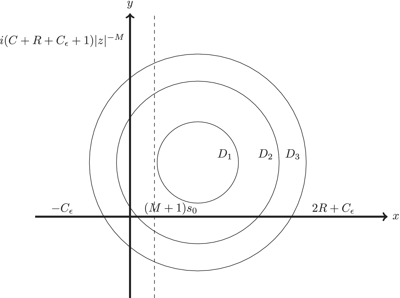
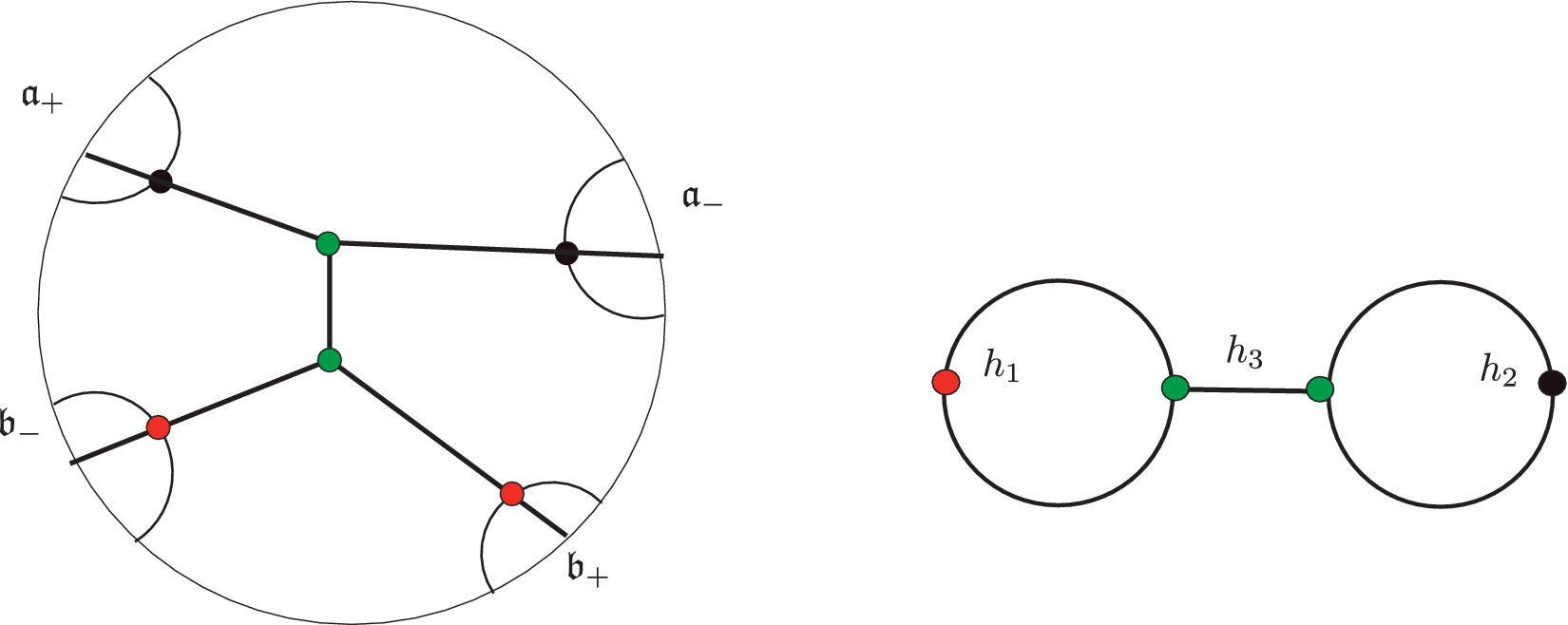
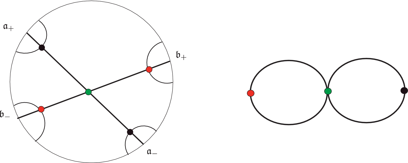
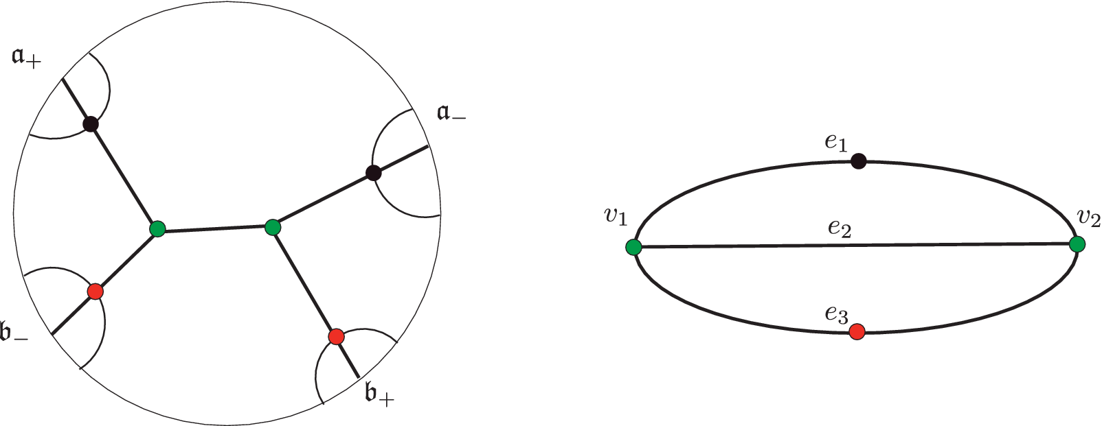


 Open access

